A model instability issue in the National Centers for Environmental Prediction Global Forecast System version 16 and potential solutions

The National Centers for Environmental Prediction (NCEP) Global Forecast System version 16 (GFSv16) encountered a few model instability failures during the pre-operational real-time parallel runs. The model forecasts failed when an extremely small thickness depth appeared at the model's lowest layer during the landfall of strong tropical cyclones. A quick solution was to increase the value of minimum thickness depth, an arbitrary parameter introduced to prevent numerical instability. This modification solved the model's numerical instability with a small impact on forecast skills. It was adopted in GFSv16 to implement this version of the operational system as planned.

Upon further investigation, it was determined that the extremely thin depth was a result of the advection of geopotential heights at the interfaces of model layers. In the Finite-Volume Cubed-Sphere (FV3) dynamical core, the horizontal winds at interfaces for advection are calculated from the layer-mean values by solving a tridiagonal system of equations in the entire vertical column based on the parabolic spline method (PSM) with high-order boundary conditions (BCs). We replaced the high-order BCs with zero-gradient BCs for the interface-wind reconstruction. The impact of the zero-gradient BCs was investigated by performing sensitivity experiments with GFSv16, idealized mountain ridge tests and the Rapid Refresh Forecast System (RRFS). The results showed that zero-gradient BCs can fundamentally solve the instability and have little impact on the forecast performances and the numerical solutions of idealized mountain tests. This option has been added to FV3 and will be utilized in the GFS (GFSv17/Global Ensemble Forecast System version 13 – GEFSv13) and RRFS for operations.

1 Introduction

The Next Generation Global Prediction System (NGGPS) of the National Centers for Environmental Prediction (NCEP) is evolving into the Unified Forecast System (UFS). It is designed to be the source system for the NOAA's operational numerical weather prediction applications and acts as the foundation for better aligning collaboration with the US modelling community (Ji and Toepfer, 2016). The Geophysical Fluid Dynamics Laboratory (GFDL) Finite-Volume Cubed-Sphere (FV3) dynamical core was chosen as the dynamical core for NGGPS in 2016 (Putman and Lin, 2007; Harris and Lin, 2013). The first major NGGPS model package was successfully implemented within the Global Forecast System (GFS). It became operational on 12 June 2019 as the GFS version 15 (referred to as GFDv15) to replace a legacy spectral model. It was further updated from version 15 to version 16 (referred to as GFSv16) on 22 March 2021 with an increased number of vertical layers and model physics upgrades.

To fully assess GFSv16's forecasting performance, both the retrospective and real-time experiments were conducted, covering part of the 2018 hurricane season and the period from 10 May 2019 to real time until the official implementation. GFSv16 outperformed GFSv15 in many aspects, including better 500 hPa height anomaly correlation scores and synoptic patterns in the medium range, a better position of relevant frontal boundaries, reduced low-level cold bias during the cool season, and improved quantitative precipitation forecast (QPF) equitable threat scores (ETSs) and biases in the medium range.

The GFS is the most important operational global weather forecast system at the NCEP/Environmental Modeling Center (EMC). Not only is it widely used around the world, but most of NCEP's forecast systems also depend on GFS products. The stability of this operational system is critical to delivering reliable real-time products to its users and downstream forecast systems. GFSv16 encountered model instability issues as several cases during the real-time parallel runs crashed before reaching a 16 d forecast length. The diagnosis of the problematic cases in GFSv16 and corresponding proposed fixes are summarized in this study. The numerical model used in GFSv16 is introduced in Sect. 2. The diagnostic results are summarized in Sect. 3. Two potential solutions to fix model instability issues are discussed in Sect. 4. Section 5 introduces the impact of proposed fixes on forecast performances with sensitivity experiments. A summary and discussion are provided in Sect. 6.

2 Model configuration upgrades

GFSv16 uses a GFDL FV3-based model as its previous version GFSv15. A detailed description of the FV3 dynamic code can be found in the published papers of the GFDL FV3 team (Lin and Rood, 1997; Lin, 2004; Harris and Lin, 2013; Putman and Lin, 2007; Harris et al., 2020a, b, 2021). Only a short summary is given here.

The cubed-sphere grid of the GFDL FV3 uses the equidistant gnomonic projection (Putman and Lin, 2007) which divides each cube edge into N segments of equal length and generates a regular mesh on a sphere by connecting non-orthogonal coordinate lines along great circles between two opposite cubic edges. This projection has the advantage of being both equal area and conformal, which allows for accurate representation of physical processes in both the horizontal and vertical dimensions.

There are two levels of time-stepping inside FV3. The inner time step (also referred to as the acoustic time step) is the integration of the dynamics along the Lagrangian surfaces, which includes computing the forward-in-time horizontal flux terms along the Lagrangian surface and the pressure-gradient force and elastic terms evaluated backwards in time. The outer time step is the vertical re-mapping process to re-grid the deformed Lagrangian surface to a reference coordinate.

The governing equations in FV3 in each horizontal layer are fully compressible flux-form vector-invariant Euler equations (Harris and Lin, 2013). The momentum flux transportation is represented as a vorticity flux and the gradient of the kinetic energy without gradients of vectors. The horizontal discretization of FV3 is derived using a two-grid system with the prognostic winds staggered on D-grid and C-grid winds used to calculate the face-normal and time-mean fluxes across the cell interfaces (Lin and Rood, 1997). The C-grid winds are interpolated from D-grid winds and then advanced a half time step as the D grid, except with lower-order fluxes, for efficiency.

The scalar advection scheme is based on the piecewise-parabolic method (PPM; Colella and Woodward, 1984) with a two-dimensional combination of one-dimensional flux methods (Lin and Rood, 1996). The same sub-grid reconstruction unlimited scheme is used for mass, potential temperature, vorticity and momentum. The transport of tracers uses a simplified monotonicity constraint (Lin and Rood, 1997) and Huynh's second-order constraint (Putman and Lin, 2007).

The evaluation of the pressure-gradient force in FV3 remains a fourth-order accuracy, is consistent with Newton's third law of motion and is achieved by finite-volume integration about a grid cell (Lin, 1997). “Vertically Lagrangian” dynamics of Lin (2004) were extended with the non-hydrostatic pressure-gradient computation of Lin (1997) and included a traditional semi-implicit solver for fast vertically propagating sound waves and gravity waves with efficient computation and great accuracy.

The Lagrangian vertical coordinate (Lin, 2004) is one unique aspect of the FV3, in which each vertical layer resembles that of a shallow water system and is allowed to deform freely during the horizontal integration. It is periodically re-mapped by vertically redistributing mass, momentum and energy to a pre-defined Eulerian coordinate to prevent severe distortion of the Lagrangian surfaces. Vertical transport occurs implicitly from horizontal transport along Lagrangian surfaces.

GFSv16 is built on 13 km quasi-uniform grids with six tiles globally, with each tile having 768 × 768 grid cells. The physics time step is 150 s in GFSv16 with the “re-mapping” time step of 75 s and the shortest acoustic time step of 12.5 s. The model uses the sigma pressure hybrid coordinate with near-surface sigma levels, blended sigma/constant pressure levels in the middle atmosphere and constant pressure levels above.

The major upgrade of GFSv16 from GFSv15 includes an increased number of vertical layers from 64 and 127 with the extended model top from 54 to 80 km and physics upgrades. The upgraded physics parameterization includes a new scheme to parameterize both stationary and non-stationary gravity waves (Alpert et al., 2019; Yudin et al., 2016, 2018), a new scale-aware turbulent kinetic-energy-based moist eddy-diffusivity mass-flux vertical turbulence mixing scheme to better represent the planetary boundary layer processes (Han and Bretherton, 2019), the improved solar radiation absorption by water clouds and the cloud-overlapping algorithm for the Rapid Radiative Transfer Model for GCMs (RRTMG) (Iacono et al., 2008) and improved GFDL cloud microphysics for computing ice cloud effective radius (Harris et al., 2020a, b; Zhou et al., 2019).

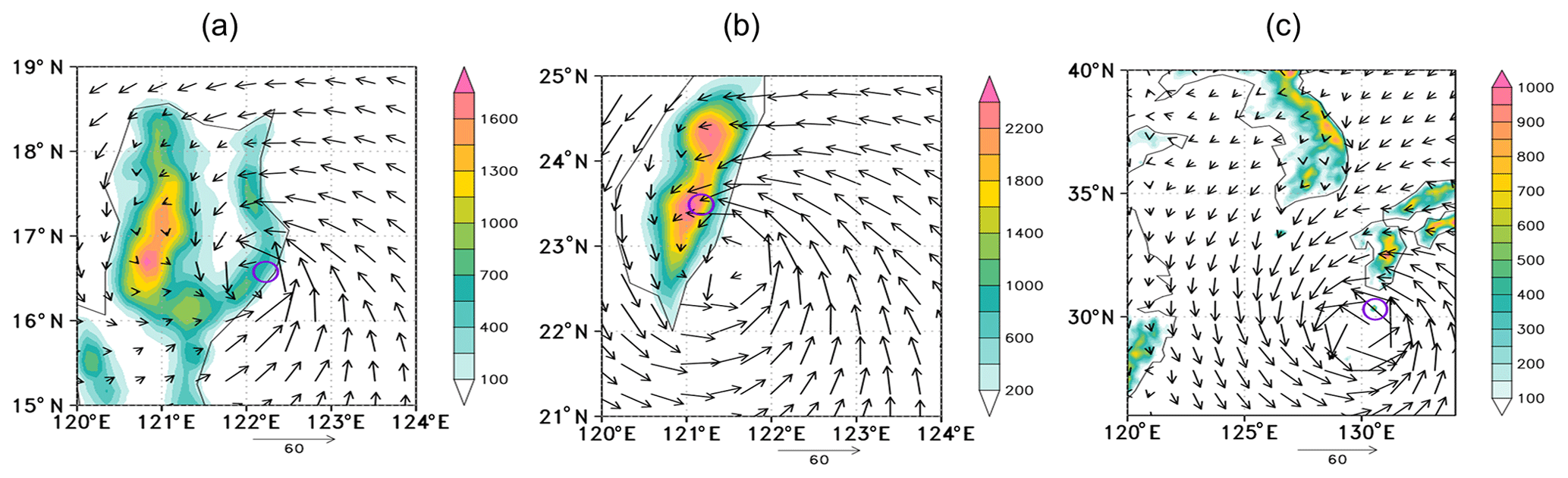
Figure 1 Horizontal wind fields (m s⁻¹) at the model lowest level before crash from the cases with the initial starting time at (a) 18:00Z (Zulu time), 22 July 2020, (b) 00:00Z, 22 September 2018 and (c) 06:00Z, 2 September 2020. The shading is terrain height (m). The open circles mark the location of the crash.

3 The study of failed cases

There were eight failed cases during the GFSv16 retrospective and real-time parallel run. They are the cases with the forecast starting times at 00:00Z, 22 September 2018, 18:00Z, 22 July 2020, 06:00Z, 2 September 2020, 06:00 and 18:00Z, 3 September 2020, 12:00Z, 4 September 2020, 06:00Z, 5 September 2020 and 00:00Z, 6 September 2020, respectively.

A series of sensitivity tests was performed to increase the model stability. Several methods available in FV3 for numerical diffusion to maintain model stability and control energy cascading were tested (Harris et al., 2021). For example, a Rayleigh damping method can be used to dampen the winds to zero with the shortest timescale (tau) at the top increasing with pressure until reaching a defined cutoff pressure level. The minimum timescale and the cutoff pressure level were tuned to apply a stronger Rayleigh damping. Other parameters such as the non-dimensional divergence damping coefficient, the Smagorinsky-type damping coefficient, and the parameters that control the sponge-layer damping to the top three layers of the model were also tuned. However, the instability issues could not be completely solved with these modifications. Although some of the cases were able to finish 16 d forecasts, not all of them became stable, indicating that further improvements were needed to address the model stability issue.

The diagnosis of these cases indicated that all model failures were related to the landfall of strong tropical cyclones. Negative layer thickness in the pressure between lower and upper interfaces or not-a-number (NaN) layer thickness in geopotential height was observed. All failures occurred at grid points located over land when the eyewall of a strong tropical cyclone made landfall from the east. For example, the forecast starting from 18:00Z, 22 July 2020 failed when a strong tropical cyclone reached the Philippine eastern coast with strong onshore winds of 40–50 m s⁻¹ (Fig. 1a). In another case, the forecast was interrupted at a grid over the Taiwan Central Mountain Range area when a strong tropical cyclone started to make landfall. The other six cases were related to tropical cyclone Haiseng (2020) when it approached the island of Yakushima south of Japan (Fig. 1c).

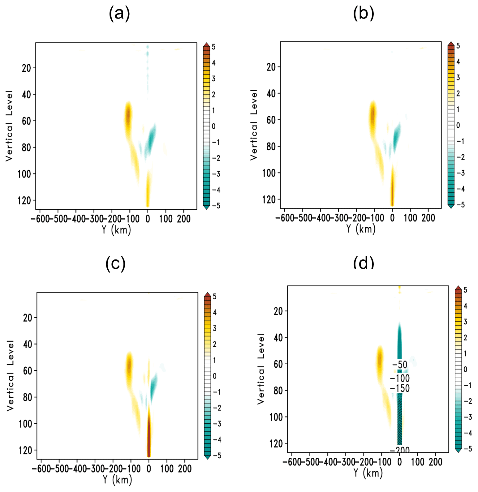
Figure 2 Vertical section of vertical velocity (m s⁻¹) through the location of the crash along with the model y-directional grids before the crash for the case with the initial forecasting time at 18:00Z, 18 July 2020. Panels (a–d) represent four, three, two and one acoustic time steps before crash, respectively. The y axis represents the number of vertical levels, with level 1 being at the top of the model.

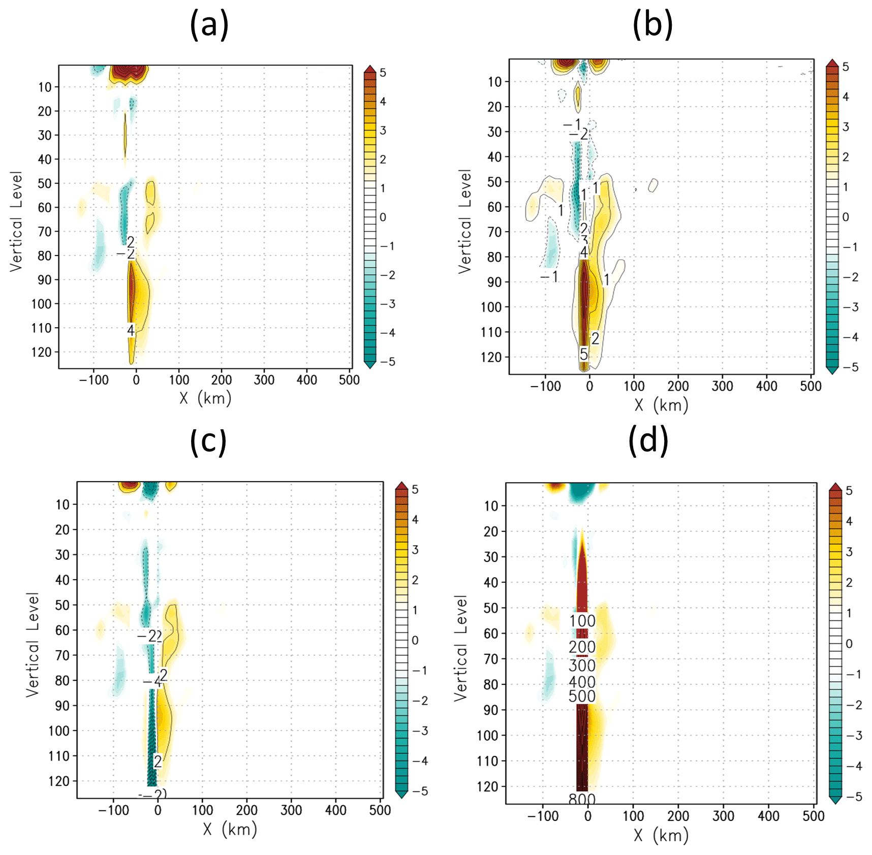
Figure 3 Like Fig. 2 except for the case with an initial starting time of 00:00Z, 22 September 2018 at each acoustic time step before the crash.

By examining the model prognostic variables in each acoustic time step (12.5 s), we found that unrealistic downdrafts occurred before the failure of the model integration. Figure 2 shows that the vertical motion at the specific grid point increases with time in the case with the initial time at 18:00Z, 18 July 2020. The updraft greater than 5 m s⁻¹ abruptly changes to an unrealistically large downdraft with an amplitude greater than 200 m s⁻¹ in one acoustic time step, which directly results in the model failure in the next time step. Figure 3 shows a similar variation of the vertical motion in the case with the initial forecast time at 00:00 UTC on 22 September 2018. Similar phenomena were observed in the other six cases related to the landfall of Haiseng (2020) (not shown).

The hydrostatic and non-hydrostatic solvers in FV3 are “switchable” at runtime through a name-list option (Harris et al., 2020a, b, 2021; Chen et al., 2013). The non-hydrostatic solver augments the hydrostatic solver by introducing the prognostic variables, namely vertical velocity w, non-hydrostatic pressure and height thickness δz. The non-hydrostatic pressure is diagnosed as a deviation with $p^{\prime }=p-p^{\ast }$, where p is the full pressure calculated from the ideal gas law:

$$\begin{array}{}\text{(1)}& p={\left(R_{\mathrm{d}}{\mathit{\theta }}_{\mathrm{v}}{\displaystyle \frac{\mathit{\delta }m}{\mathit{\delta }z}}\right)}^{\mathit{\gamma }}.\end{array}$$

δm and δz are the mass and height thickness. θ_v = $T_{\mathrm{v}}(\frac{p_{\mathrm{0}}}{p}{)}^{\mathit{\kappa }}$ is virtual potential temperature where p₀ = 1 Pa in FV3, κ = $(\mathrm{1}+\frac{C_{\text{vm}}}{R_{\mathrm{d}}(\mathrm{1}+\mathit{ϵ}{q}_{\mathrm{v}})}{)}^{-\mathrm{1}}$, and T_v is the “condensate-modified” virtual temperature. R_d is the gas constant for dry air. The parameter γ = $(\mathrm{1}+\mathit{\kappa }{)}^{-\mathrm{1}}$. C_vm is the “moist” specific heat capacities under constant volume and q_v is specific humidity.

Non-hydrostatic pressure perturbation p^′ and w in the Lagrangian vertical coordinates are solved using a semi-implicit solver in which the fully implicit time-difference scheme yields a tridiagonal matrix system of equations for vertical velocity w. This system requires coefficients and weights related to p^′ and layer thickness δz to solve w with the Thomas algorithm (Thomas, 1949).

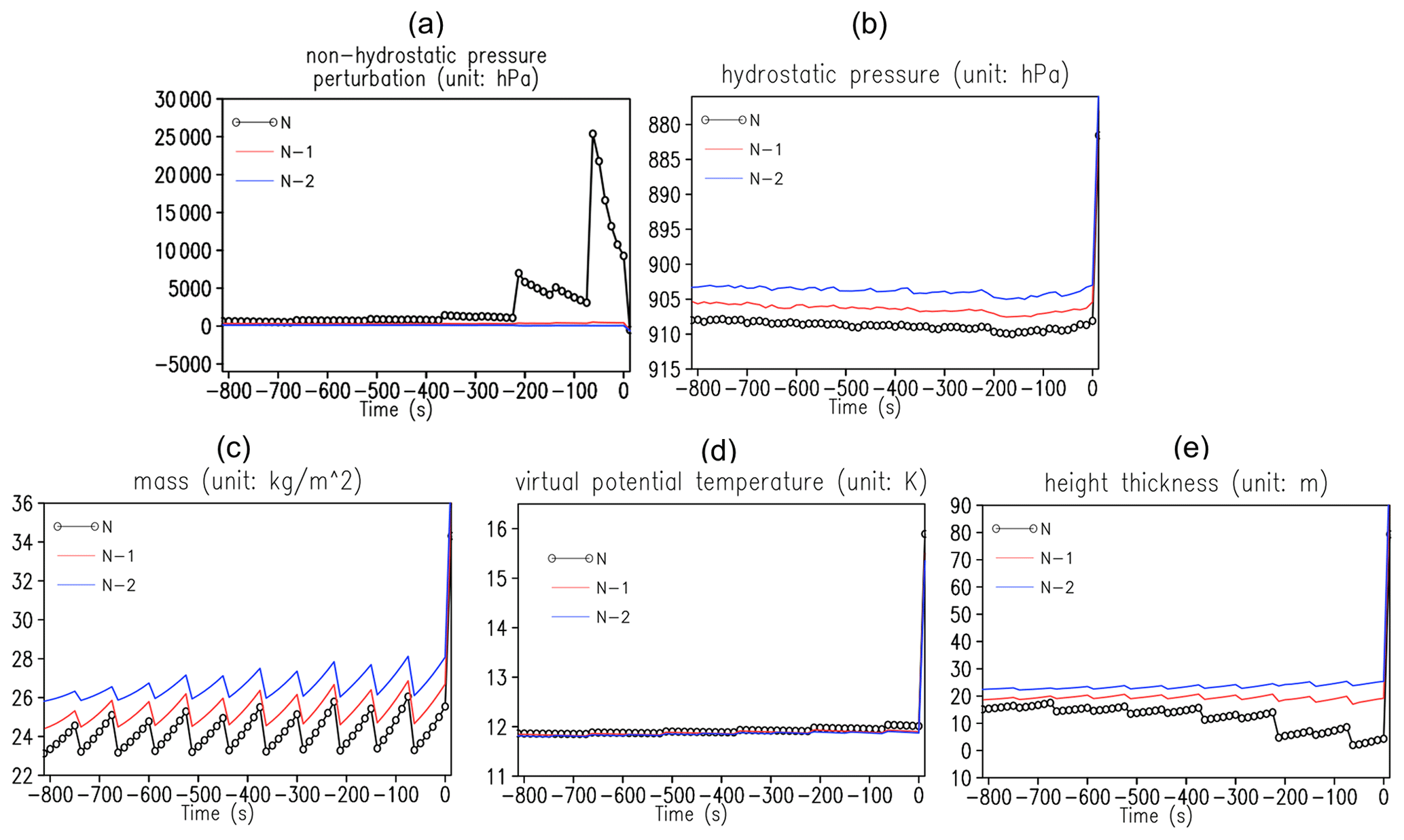
Figure 4 The time series of (a) non-hydrostatic pressure, (b) hydrostatic pressure, (c) mass, (d) virtual potential temperature and (e) thickness depth in height at the crash grid for the case with the initial starting time 18:00Z, 18 July 2020. The black curves represent the model's lowest level (marked by N), while the blue and red curves represent the second- and third-lowest levels (marked with N−1 and N−2). The open circle marks each acoustic time step in the time series.

All relevant variables before the crash time including p^∗, p, θ_v, δz, and the mass δm to calculate w were investigated. In the FV3 model, all the algorithms are formulated in a finite-volume manner. This means that the above variables of interest are represented as cell or layer means. Figure 4 shows that θ_v and δm remain reasonable and consistent before the crash (Fig. 4c and d). The unrealistic value of the full pressure (larger than 5000 hPa) appears at the model's lowest level at about 200 s before the model crash (Fig. 4a), while the hydrostatic pressure remains reasonable (about 900 hPa) with time (Fig. 4b). The slight discontinuity of these variables every six acoustic time steps is a result of the vertical re-mapping process. GFSv16 has 127 vertical layers, with the lowest layer about 20 m thick on average. The value of δz close to zero 200 s prior to the crash is quite unusual (Fig. 4e). The unrealistically increased p^′ and the full pressure at the lowest level before the crash come from the occurrence of extremely small δz but computed from the ideal gas law formula. Extremely large downdrafts are generated through the non-hydrostatic semi-implicit solver from p^′, which eventually leads to the model failure. The model instability is a result of the presence of extremely small δz at the lowest model level.

The calculation of δz, the vertical difference of geopotential height z between the Lagrangian surfaces before the non-hydrostatic adjustment, was investigated. The forward-in-time advective processes are performed to generate the partially updated z before the non-hydrostatic adjustment in the FV3 dynamics. Note that the update of z through advection processes does not directly solve an equation for the volume of a grid cell (δz), and it is forward in time as the sum of the advective height flux along with the Lagrangian interfaces and the vertical distortion of the surfaces by the gradient of z. The previous study found that the advection of δz created excessive noise near steep topography (Harris et al., 2021), and it was more difficult to guarantee the kinematic surface condition without perpendicular flow to the surface with the advection of δz.

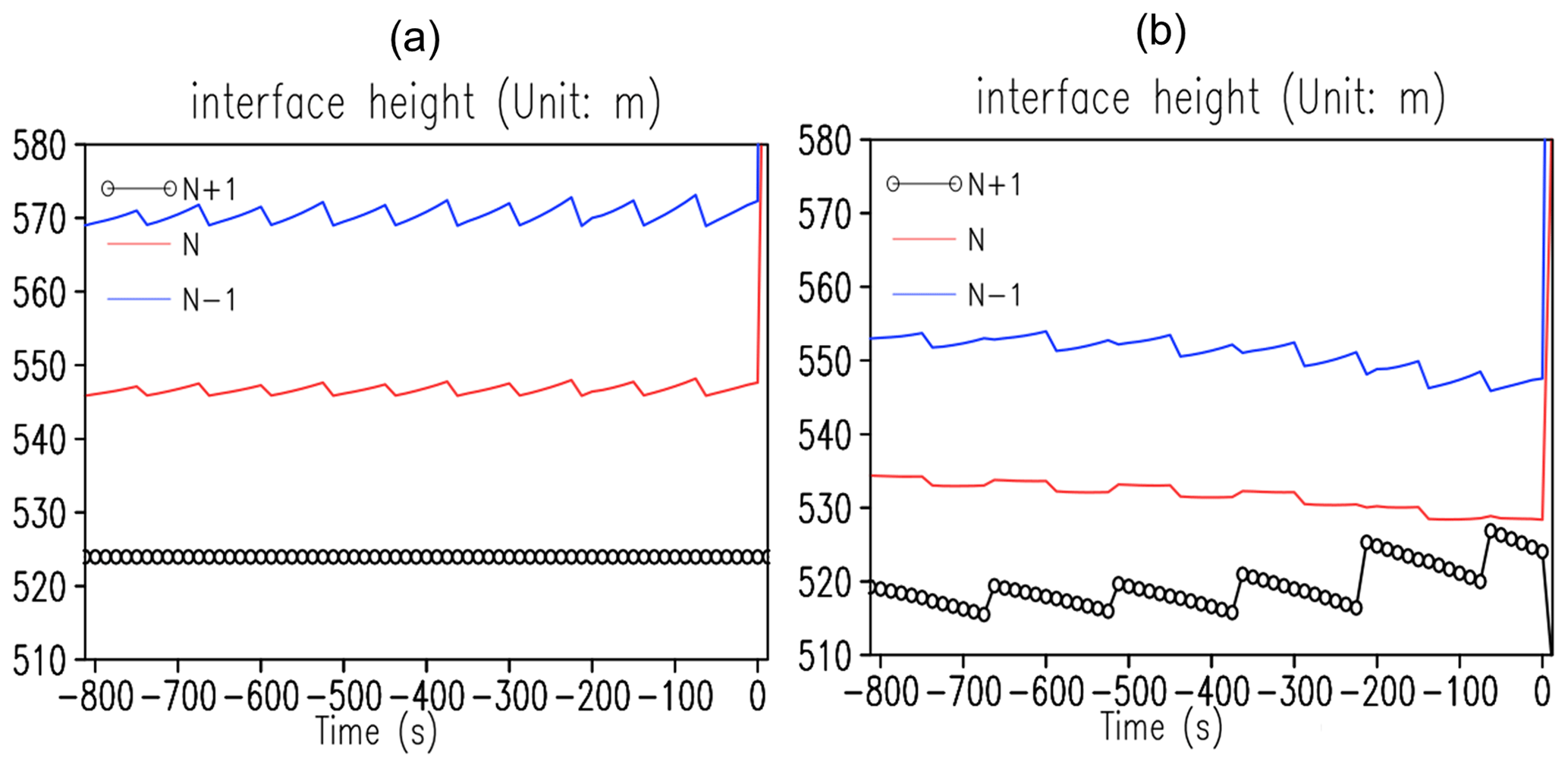
Figure 5 Like Fig. 4 except for the geopotential height at the model's three lowest interface layers (marked as N+1, N and N−1, respectively) (a) before and (b) after the advection procedure for the case with the initial starting time 18:00Z, 18 July 2020.

To advance z on the interfaces, the advection winds are interpolated from layer means onto the layer interfaces. Figure 5 shows the time series of z at the crash location before and after the advection process. The value of z at the lowest level before advection remains constant as it is the height of the topography (Fig. 5a). After advection, there is a significant change, and it becomes close to the value of z at the second-lowest level (Fig. 5b), starting around 200 s before the crash. There are no noticeable changes in z at the second- and third-lowest levels both before and after the advection. As δz at the lowest level represents the difference between the height at the two lowest interfaces, the advection process at the lowest level is responsible for the decreased thickness depth seen in Fig. 4e.

4 Potential solutions

The forward-in-time advection of geopotential height is a part of the acoustic time step in which the Lagrangian surface is allowed to freely deform. An artificial limiter is defined as the minimum thickness depth after the geopotential height advection to enhance its monotonicity in the vertical. This limiter is defined as dz_min in FV3 with 2 m as the default in FV3. It only takes effect when the thickness of geopotential occurring in the model is smaller than the default value. We found that increasing this limiter value from 2 to 6 m can effectively avoid model crashes. All eight cases can finish 16 d forecasts with this modification.

To examine whether increasing this artificial limiter violates general model states in GFSv16, the possibility of δz reaching the minimum thickness depth of 6 m was investigated in both crash cases and successful cases. The successful cases were randomly selected from the retrospective runs among the cases that can complete 16 d forecasts successfully. There were no extremely small δz values in any grids from randomly selected successful cases. δz less than 6 m likely only occurred at the breakpoint in crash cases, and this artificial limiter is only used in very rare situations. Forecast-only experiments also showed that this fix had very little impact on the forecast skill. Since any changes in the forecast performance were not desirable at the final retrospective test stage for the implementation of GFSv16, this method was considered a suitable temporary fix for GFSv16. It was adopted for the GFSv16 implementation, and this fix allowed GFSv16 to be implemented at the time.

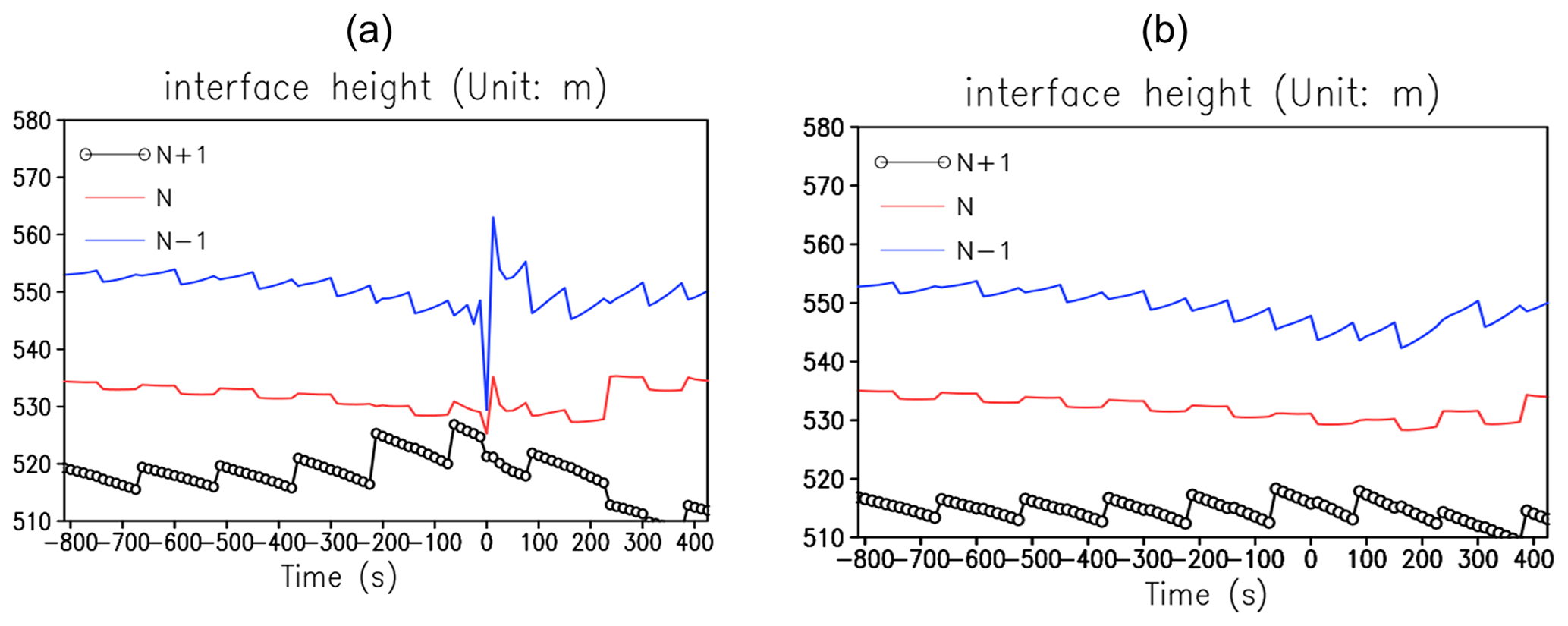
Figure 6 The time series of the geopotential height at the model's three lowest interface layers (marked as N+1, N and N−1, respectively) after the advection at the original crash location in the sensitivity experiments with proposed fixes: (a) increased dz_min from 2 to 6 and (b) zero-gradient BCs for the case with the initial starting time 18:00Z, 18 July 2020.

A sensitivity experiment was performed by restarting the model about 1 h before the crash with increased minimum thickness depth. The geopotential height after the advection was forced to be greater than the artificial limiter. The abrupt change in the geopotential height was observed at the original crash location and time, and then it backed to a normal range after several acoustic time steps (Fig. 6a). The model can successfully finish 16 d forecasts. The increased minimum thickness depth can prevent the model from crashing, but it does not fundamentally solve the model instability issue. In addition, this arbitrary limiter should be used with caution, and the height of the model's lowest level should be considered to select a reasonable value for the limiter.

The advection process to update z in FV3 was examined since the model instability issue likely originated from the advection of z at the model's lowest level. To update z, the advection winds and vertical velocity are reconstructed from layer means onto the layer interfaces by solving a tridiagonal system of equations based on the parabolic spline method (PSM, Zerroukat et al., 2006).

The following equation represents the relationship between the interface value ${\widehat{q}}_{i-\frac{\mathrm{1}}{\mathrm{2}}}$ and layer-mean value ${\stackrel{\mathrm{‾}}{q}}_i$ ($i=\mathrm{1},\mathrm{2},\mathrm{\dots }N$) from the model top to the lowest level in a computational one-dimensional discretized domain with PSM (Zerroukat et al., 2006):

$$\begin{array}{}\text{(2)}& \begin{array}{rl}{\displaystyle \frac{\mathrm{1}}{h_i}}{\widehat{q}}_{i-\frac{\mathrm{1}}{\mathrm{2}}}& +\mathrm{2}\left({\displaystyle \frac{\mathrm{1}}{h_i}}+{\displaystyle \frac{\mathrm{1}}{h_{i+\mathrm{1}}}}\right){\widehat{q}}_{i+\frac{\mathrm{1}}{\mathrm{2}}}+{\displaystyle \frac{\mathrm{1}}{h_{i+\mathrm{1}}}}{\widehat{q}}_{i+\frac{\mathrm{3}}{\mathrm{2}}}\\ & =\mathrm{3}\left({\displaystyle \frac{\mathrm{1}}{h_i}}{\stackrel{\mathrm{‾}}{q}}_i+{\displaystyle \frac{\mathrm{1}}{h_{i+\mathrm{1}}}}{\stackrel{\mathrm{‾}}{q}}_{i+\mathrm{1}}\right),\end{array}\end{array}$$

where h_i is the spatial interval between two interfaces h_i = $z_{i+\frac{\mathrm{1}}{\mathrm{2}}}-z_{i-\frac{\mathrm{1}}{\mathrm{2}}}$ ($i=\mathrm{1},\mathrm{2}\mathrm{\dots }N$) and q represents horizontal wind components u and v here. Equation (2) defines a linear system of equations for the unknown interface values ${\widehat{q}}_{i-\frac{\mathrm{1}}{\mathrm{2}}}$ in terms of the layer-mean values ${\stackrel{\mathrm{‾}}{q}}_i$. Boundary conditions are required to close the problem. FV3 uses the following equations for the upper and lower boundaries to solve the horizontal winds at the model interfaces as a problem of a tridiagonal system:

$$\begin{array}{}\text{(3)}& {\displaystyle }\begin{array}{rl}& g_{\mathrm{1}}(g_{\mathrm{1}}+\mathrm{0.5}){\widehat{q}}_{\frac{\mathrm{1}}{\mathrm{2}}}+[\mathrm{1}+g_{\mathrm{1}}(g_{\mathrm{1}}+\mathrm{1.5}\left)\right]{\widehat{q}}_{\frac{\mathrm{3}}{\mathrm{2}}}\\ & =\mathrm{2}{g}_{\mathrm{1}}(\mathrm{1}+g_{\mathrm{1}}){\stackrel{\mathrm{‾}}{q}}_{\mathrm{1}}+{\stackrel{\mathrm{‾}}{q}}_{\mathrm{2}},\end{array}\text{(4)}& {\displaystyle }\begin{array}{rl}& [\mathrm{1}+g_N(g_N+\mathrm{1.5}\left)\right]{\widehat{q}}_{N-\frac{\mathrm{1}}{\mathrm{2}}}+g_N(g_N+\mathrm{0.5}){\widehat{q}}_{N+\frac{\mathrm{1}}{\mathrm{2}}}\\ & ={\stackrel{\mathrm{‾}}{q}}_{N-\mathrm{1}}+\mathrm{2}{g}_N(\mathrm{1}+g_N){\stackrel{\mathrm{‾}}{q}}_N,\end{array}\end{array}$$

with $g_{\mathrm{1}}=h_{\mathrm{2}}/h_{\mathrm{1}}$ and $g_N=h_N/h_{N-\mathrm{1}}$ with level 1 at the model top and level N at the lowest level.

We proposed using zero-gradient BCs, i.e. $\frac{\mathrm{d}q}{\mathrm{d}z}=\mathrm{0}$ at the endpoints z_½ and z_N+½ corresponding to an assumption of zero slope there. Applying these zero-gradient BCs leads to

$$\begin{array}{}\text{(5)}& {\displaystyle }\mathrm{2}{\widehat{q}}_{\frac{\mathrm{1}}{\mathrm{2}}}+{\widehat{q}}_{\frac{\mathrm{3}}{\mathrm{2}}}=\mathrm{3}{\stackrel{\mathrm{‾}}{q}}_{\mathrm{1}},\text{(6)}& {\displaystyle }{\widehat{q}}_{N-\frac{\mathrm{1}}{\mathrm{2}}}+\mathrm{2}{\widehat{q}}_{N+\frac{\mathrm{1}}{\mathrm{2}}}=\mathrm{3}{\stackrel{\mathrm{‾}}{q}}_N.\end{array}$$

The original BCs used in FV3 as shown in Eqs. (3) and (4) are named high-order BCs hereafter, in contrast to the zero-gradient BCs we proposed.

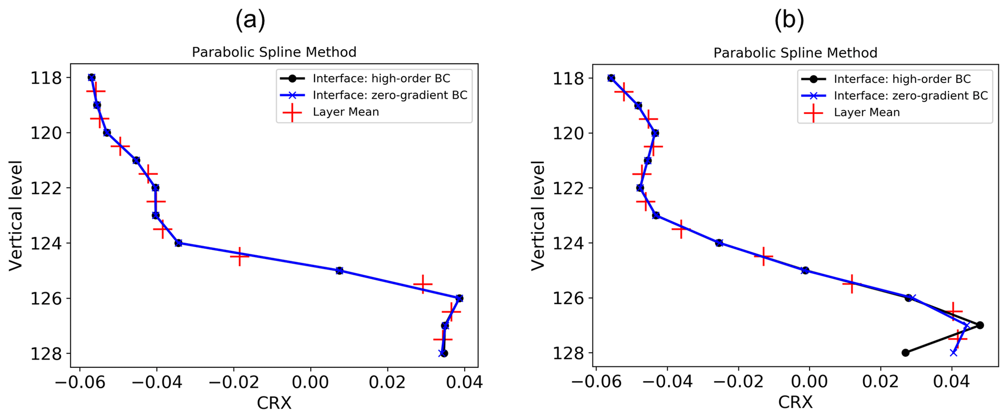
Figure 7 The vertical profile of Courant numbers on the x axis ($c_x=t\cdot u/\mathrm{\Delta }x)$ at two grids with (a) smaller and (b) larger vertical gradients. The red cross represents the layer-mean value, while black and blue represent the interface values reconstructed with high-order BCs and zero-gradient BCs.

The comparison of the vertical profiles with two different BCs shows that the reconstructed winds are similar in these two types of BCs when the vertical shear of the layer-mean winds in the lower levels is relatively small (Fig. 7a). With larger vertical shear, the overshooting and undershooting of the reconstructed winds at the lowest two layers are more evident by using higher-order BCs than zero-gradient BCs, while interior winds remain similar (Fig. 7b). The vertical shears of interface winds at the lowest several layers are smaller with zero-gradient BCs than with high-order BCs.

With the application of the zero-gradient BCs, all originally crashed cases can finish 16 d forecasts successfully. A sensitivity experiment was performed similarly for zero-gradient BCs. Figure 6b shows that applying the zero-gradient BCs avoids unrealistic δz values. No extremely small δz was found during the model integration. This method is better than increasing the artificial thickness depth limiter as it fundamentally solves the occurrence of unrealistic δz values at the model's lowest level.

PSM is third-order accurate in space for a non-uniform grid and fourth-order accurate for a uniform grid (Zerroukat et al., 2006). The reconstructed winds at the BCs with high-order BCs may retain a relatively higher accuracy. However, it can be worse in the case of sharp/under-resolved gradients with significant overshoots/undershoots due to a larger degree of freedom. Constraints are usually required for the reconstruction to prevent overshoots/undershoots with respect to the layer-mean values (Shchepetkin and McWilliams, 1998; Zerroukat et al., 2006). Our method is to reduce the order of the reconstruction polynomial for BCs. It is worth noting that the zero-gradient condition is only used at the model's upper and lower edge levels. The parabolic spline as the reconstructed function remains valid for the inner layers. In addition, the reconstructed horizontal winds are only used for the advection of geopotential height. The revised BCs do not impact the layer-mean prognostic wind fields directly.

5 Sensitivity experiments with zero-gradient BCs

The impact of zero-gradient BCs on forecast performance was investigated with different model configurations. The experiment design and results are discussed including idealized mountain ridge tests and real-case tests with the same configuration as GFSv16 and the high-resolution regional application in EMC.

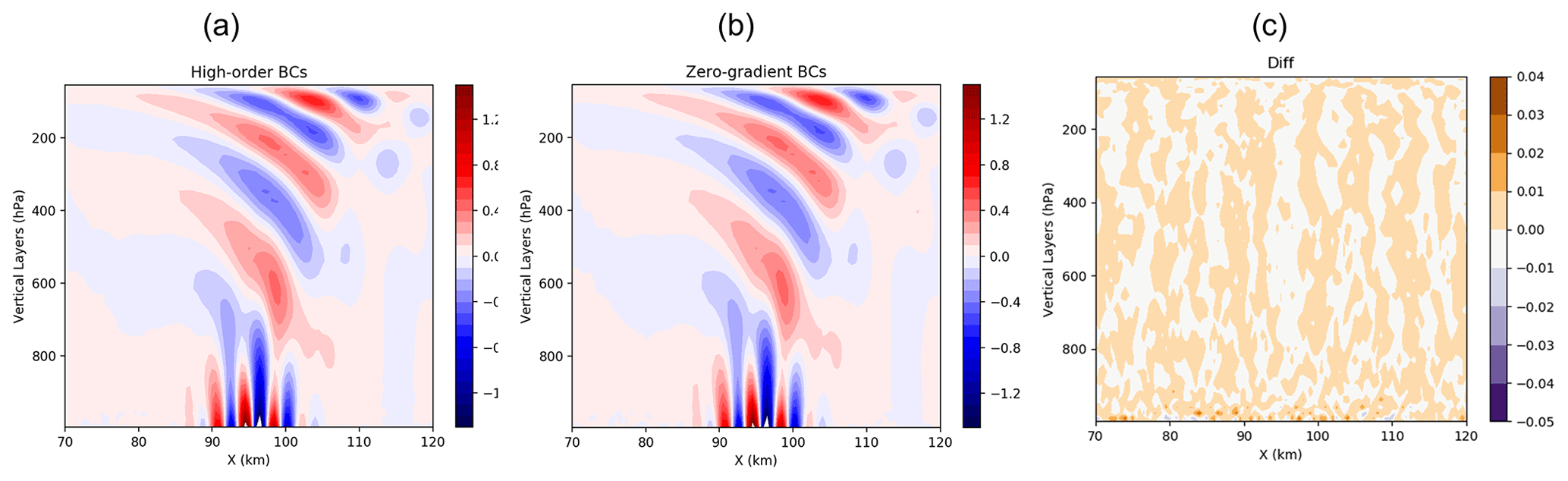
Figure 8 Cross sections of vertical velocity (m s⁻¹) along the Equator for orographic mountain ridges on the Earth (quasi-two-dimensional ridge in a barotropic zonal flow). The x axis is measured in kilometres to represent distance and the y axis is the vertical coordinate in pressure (hPa) in (a) the control and (b) the sensitivity run with zero-gradient BCs. Panel (c) shows the difference between these two runs.

The mountain waves could be sensitive to the model's lower-boundary conditions (Smith, 2007). The impact of the BC change on the geopotential height advection on the mountain waves was investigated. An idealized mountain ridge test with an adiabatic condition, a uniform flow of 8 m s⁻¹ over a ridge mountain, was performed. This is a modified version of the Dynamical Core Model Intercomparison Project (DCMIP) case 2.1 with a quasi-two-dimensional mountain ridge with a ridge height of 250 m (Ullrich et al., 2017). Instead of assuming a small Earth, the idealized mountain ridge experiment was tested on a doubly periodic domain. The model top is 50 hPa with a horizontal resolution of 500 m. Zero-gradient BCs are utilized at the upper and lower boundaries in the sensitivity experiment. The mountain wave patterns are similar in these two experiments. Although slightly larger at the lowest levels, the difference is negligible throughout the entire domain (Fig. 8). At both the upper and lower boundaries of the model, identical boundary condition methods are implemented. However, the damping applied to absorb vertically propagating waves may have a lesser effect at the upper boundary. This can be attributed to two forms of damping utilized, namely Rayleigh damping, which reduces wind speed to zero within a specific timescale, and a sponge damping layer that employs second-order damping to divergence, vorticity, mass and w flux in the top three layers of the model.

A group of sensitivity experiments was performed by using GFSv16 as the control. A sensitivity experiment was performed by replacing high-order BCs in the control with zero-gradient BCs at both the lower and upper boundaries of the model to reconstruct horizontal winds with PSM; 10 d forecasts were compared with initial times from June to October 2020 every 5 d with 00:00Z only. The EMC Global NWP Model Verification Package was used for the verification (Yang et al., 2006). This verification package is a standard evaluation tool for the GFS upgrade and implementation with verification scores comparing gridded model data to both point-based rawinsonde and surface station observations and GFS gridded analysis. The model forecast statistics in terms of the root mean square error (RMSE), bias and anomaly correlation for conventional variables and tropical cyclone intensity and track forecasts over the Atlantic, eastern Pacific, and western North Pacific and precipitation threat skill scores over the CONUS. The comparison of these forecast verification metrics shows that the sensitivity experiments with zero-gradient BCs have similar forecast performances without significant differences to those of GFSv16 with high-order BCs (not shown).

The Rapid Refresh Forecast System (RRFS) is another important FV3-based UFS application in EMC. It is the NOAA next-generation convection-allowing, rapidly updated ensemble prediction system of a limited area (the continental US, CONUS) (Black et al., 2021), currently scheduled for operational implementation in 2024. The operational configuration features a 3 km grid spacing covering North America and includes forecasts every hour out to 18 h, with extensions to 60 h four times per day at 00:00, 06:00, 12:00 and 18:00Z. Each forecast is planned to be composed of 9–10 members.

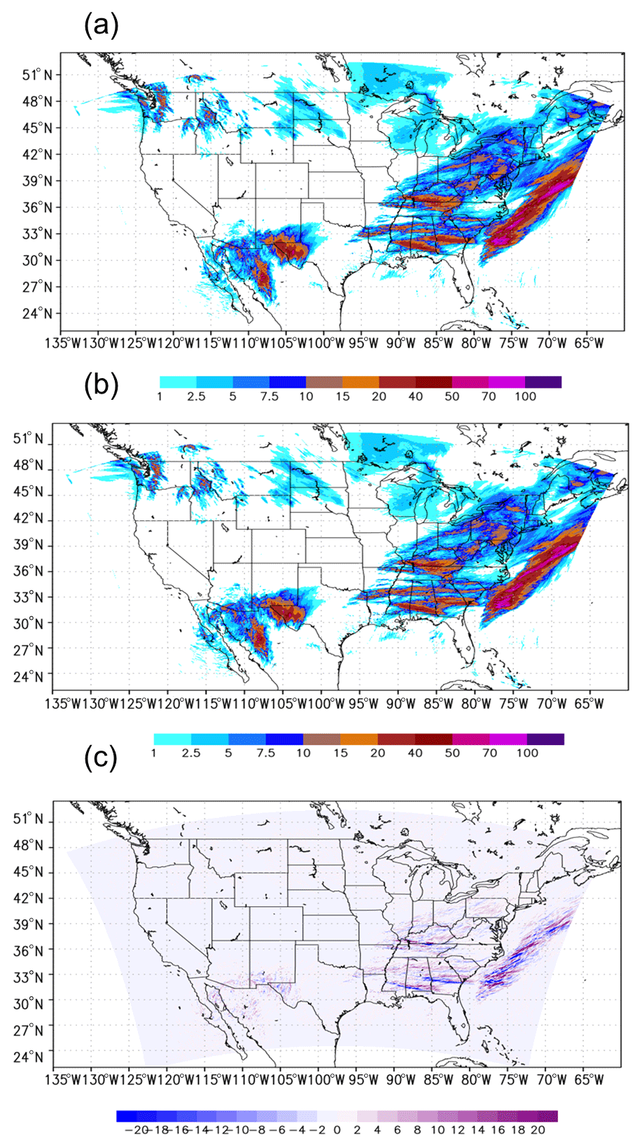
Figure 9 The 24 h precipitation (mm) from 12 to 36 h in (a) the control and (b) the sensitivity run with zero-gradient BCs. Panel (c) shows the precipitation difference between these two runs. The control run has the same configuration as the ensemble member one in the RRFS, with the initial starting time on 00:00Z, 2 March 2020.

The impact of the zero-gradient BCs on the high-resolution forecasts was also investigated based on the RRFS configuration. The ensemble members with the Mellor–Yamada–Nakanishi–Niino (MYNN) (Nakanishi, 2001; Olson et al., 2019) planetary boundary layer (PBL) and Thompson microphysics (MP) scheme were used as the control to investigate the impact of zero-gradient BCs. Figure 9 shows that the precipitation distribution from 12 to 36 h in the experiment with zero-gradient BCs resembles that in the control. The use of zero-gradient BCs does not significantly change the forecast results for high-resolution forecasts.

6 Summary and discussion

GFS is one of the most important operational global weather forecast systems at NCEP/EMC. The stability of GFS on model integration is as important as its forecast skills for delivering dependable real-time products to its users and downstream forecast systems. The model instability issue of GFSv16 caught our attention when several cases in its real-time parallel runs failed to finish 16 d forecasts. The analysis of these cases showed that the model integration was interrupted after the presence of a very thin layer depth corresponding to a largely deformed layer surface at the model's lowest level in tropical cyclones during the landfall after the advection of geopotential height.

An artificial limiter is defined in FV3 to ensure that the minimum layer depth in FV3 after the advection is not less than a default value to maintain the monotonicity of geopotential height in the vertical. Sensitivity tests showed that increasing the value of this artificial parameter from the default values of 2 to 6 m can fix the model instability issue. An abrupt change in geopotential height at the model's lowest interface was still observed with an increased value of the limiter, but all previously crashed cases can finish 16 d forecasts. This method was effective at solving the model instability issue and was adopted to GFSv16 so that the GFSv16 can be implemented as scheduled. Nevertheless, this method lacks a scientific foundation, and the root reason corresponding to the model instability remains unknown.

Further investigation suggested that the presence of an extremely thin layer at the model's lowest layer was related to the reconstruction of interface winds from layer-mean winds for the advection of geopotential height along the Lagrangian surfaces. In FV3, the horizontal winds are calculated from layer means onto the layer interfaces by solving a tridiagonal system of equations based on PSM (Zerroukat et al., 2006) with high-order BCs. It was found that the high-order BCs easily produce overshoots or undershoots in areas with large vertical wind shear. The lower boundary in a landfall tropical cyclone was a perfect condition for the occurrence of overshoots/undershoots with high-order BCs, which led to a heavily distorted Lagrangian surface and triggered unstable conditions. The change in BCs from high-order to zero gradients at the lowest interface removed spurious undershoots/overshoots near steep terrain with vertical wind shears, thus avoiding a distorted geopotential height interface so that the model remains in stable conditions.

The impact of the zero-gradient BCs for the tridiagonal system on the forecast results was very minor. The zero-gradient condition for BCs was only valid at the model's lowest/highest interface. The reconstructed horizontal wind profile at sub-grids remained a parabolic spline as defined in terms of the layer-mean values. In addition, the reconstructed interface horizontal winds were only used in the advection of geopotential height. The zero-gradient BCs did not impact the prognostic layer-mean wind fields directly. The zero-gradient BCs had been committed to the Unified Forecast System (UFS) as an alternative method for the forward-in-time advection of geopotential height.

Even though the model instability issue only was found during the landfall of tropical storms in GFSv16, it could be the case in any situations with strong vertical shear of winds at the lower and upper boundaries. It was found that the zero-gradient BCs can effectively improve the model forecast stability for RRFS in non-tropical cyclone cases. This option has been included in the RRFS package for the real-time parallel runs. For the GFS, the artificial limiter used in GFSv16 will be replaced by the option of zero-gradient BCs to stabilize the model forecasts in the next-generation coupled GFSv17/Global Ensemble Forecast System (GEFSv13). RRFS and GFSv17/GEFSv13 target operational implementation in 2024 and 2025.