An internal solitary wave forecasting model in the northern South China Sea (ISWFM-NSCS)

Internal solitary waves (ISWs) are a ubiquitous phenomenon in the dynamic ocean system, which play a crucial role in driving transport through turbulent mixing. Over the past few decades, numerical modelling has become a vital approach to investigate the generation mechanism and spatial distribution of ISWs. The northern South China Sea (NSCS) has been treated as a physical oceanographic focus of ISWs in massive numerical studies since the last century. However, there has been no systematic evaluation of a reliable three-dimensional (3D) model about accurately reproducing ISW characteristics in the NSCS. In this study, we implement a 3D ISW forecasting model in the NSCS and quantitatively evaluate the requirements of factors (i.e. model resolution, tidal forcing, and stratification selection) in accurately depicting ISW properties by comparison with observational data at a mooring station in the vicinity of the Dongsha Atoll. Firstly, the 500 m resolution model can basically reproduce the principal ISW characteristics, while the 250 m resolution model would be a better solution to identify wave properties, specifically increasing 40 % accuracy of predicting characteristic half-widths. Nonetheless, a 250 m resolution model spends nearly 5-fold the computational resources of a 500 m resolution model in the same model domain. Compared with the former two, the model with a lower resolution of 1000 m severely underestimates the nonlinearity of ISWs, resulting in an incorrect ISW field in the NSCS. Secondly, the model with 8 (or 13) primary tidal constituents can accurately reproduce the real ISW field in the NSCS, while the one with four main harmonics (M2, S2, K1 and O1) would underestimate averaged wave-induced velocity for about 38 % and averaged mode-1 wave amplitude for about 15 %. Thirdly, the model with the initial condition of field-extracted stratification gives a better performance in predicting some wave properties than the model with climatological stratification, namely 13 % improvement of arrival time and 46 % improvement of characteristic half-width. Finally, background currents, spatially varying stratification and external (wind) forcing are discussed to reproduce a more realistic ISW field in the future numerical simulations.

1 Introduction

Numerical simulations, one of the most important approaches to investigate internal solitary waves (ISWs) in the world's oceans, have been gradually developed from two-dimensional (2D, e.g. Du et al., 2008; Buijsman et al., 2010a) to three-dimensional (3D, e.g. Zhang et al., 2011; Alford et al., 2015) over the past few decades. The South China Sea (SCS), the largest marginal sea in the northwest Pacific, has been commonly known as an active region of ISWs via massive in situ observations (cf. Ramp et al., 2004, 2019; Farmer et al., 2009, 2011) and number of remote sensing images (cf. Liu and Hsu, 2004; Zheng et al., 2001, 2007). Although the vertical structure and horizontal distribution on the sea surface of ISWs can be nicely illustrated by field measurements at sparse sites and satellite images, respectively, they are still of limited value for telling a complete story of ISWs in the entire northern SCS (NSCS). Complementary to in situ and remote-sensing observations, numerical models can give a comprehensive characterization in the ISW field in the case of realistic initial and boundary conditions. Hence, we take NSCS as an example to introduce a high-performance ISW forecasting model and quantitatively evaluate requirements of model configurations (i.e. resolution, tidal forcing and stratification selection) for accurately reproducing a real ISW field.

With the development of higher performance computing facilities, a variety of 3D realistic numerical models with structured and unstructured grids were established for simulating ISWs in the NSCS (see Table 1), such as MITgcm (Vlasenko et al., 2010), SUNTANS (Zhang et al., 2011) and FVCOM (Lai et al., 2019). Meanwhile, the model capabilities have been continuously improved (Simmons et al., 2011). Specifically, the model resolution was effectively enhanced from 250–1000 (Δx–Δy) m (Guo et al., 2011) in a limited domain to 150–300 m in a large domain including the entire NSCS (Zeng et al., 2019). From past to present, the barotropic tidal forcing dataset TOPEX/Poseidon Solution (TPXO; Egbert and Erofeeva, 2002) and climatological stratification dataset World Ocean Atlas (WOA; Locarnini et al., 2019) have been updated with higher resolutions both in the horizontal and vertical, providing more realistic and precise boundary and initial conditions in the model configurations. Although it is commonly known that a higher-resolution model can tell a more complete story of ISWs, the usage of computational resources is worth considering. Thus, what resolution of model is needed to give an accurate depiction of ISW fields and simultaneously save the computational cost is still a question.

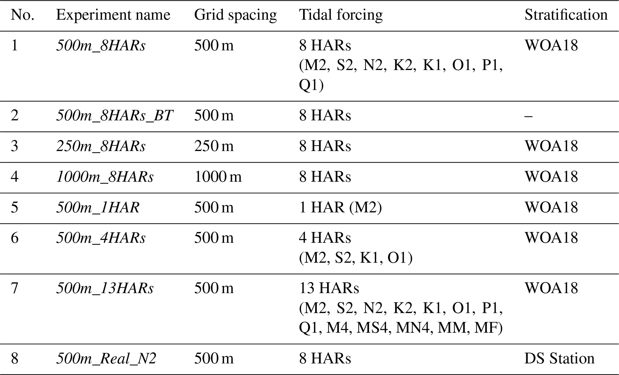
Table 1 Summary of previous 3D non-hydrostatic models for internal solitary waves in the northern South China Sea, which are discussed in the text. Further details can be found in the references. HARs is the abbreviation for harmonics.

Even though numbers of previous in situ observations have shown the four barotropic tidal constituents (M2, K1, O1 and S2) are dominant at the Luzon Strait (Zhao and Alford, 2006; Farmer et al., 2009), the other barotropic tidal constituents (e.g. N2, K2, P1 and Q1) are also non-negligible (Beardsley et al., 2004). Historically, numerical simulations with different numbers of tidal constituents have been widely employed to investigate the physical dynamics of ISWs in the NSCS, i.e. single K1 harmonic (Li, 2014), four tidal harmonics (Buijsman et al., 2010b), and eight primary tidal harmonics (Alford et al., 2015; Jin et al., 2021). Among these, eight tidal constituents were most commonly applied in the 3D models. However, other tidal constituents, such as M4, MS4, MN4, MM and MF, have yet to be considered. The questions are whether a single tidal constituent can reproduce a real ISW field, and, if not, how many tidal constituents are required to run an accurate 3D realistic ISW model.

Apart from resolution and tidal forcing, stratification selection is also an important factor in improving model accuracy. A horizontally homogenous stratification profile was normally implemented as an initial condition in a 3D realistic model (cf. Zhang et al., 2011; Lai et al., 2019). Specifically, a domain average of the climatological dataset (WOA) is one of the most common options (Vlasenko et al., 2010; Zeng et al., 2019), since the in situ observational data are relatively inaccessible. Once the field data at an isolated mooring station are available, are they a better choice than the climatological data to be the model's initial condition? What if the mooring is near-field (in the vicinity of the Luzon Strait, the ISW generation site) or far-field (e.g. in the deep basin or over the continental slope and shelf)?

In this paper, we attempt to introduce a high-performance ISW forecasting model and evaluate the roles of different resolutions, initial and boundary conditions in accurately reproducing ISWs via a series of sensitivity 3D non-hydrostatic numerical simulations. The paper is structured as follows. In Sect. 2, configurations of the 3D forecasting model are introduced, as well as the simultaneous remote sensing images and in situ observations. The model calibrations are presented in Sect. 3. In Sect. 4, we quantitatively illuminate the requirements of model resolutions, tidal constituents and initial stratification selection for a reliable 3D ISW forecasting model. Discussion and conclusions follow in Sect. 5.

2 Data and methods

To characterize the real ISW field in the NSCS, we implement an ISW forecasting model (ISWFM-NSCS) and compare the modelled wave properties on the continental slope with those observed at in situ mooring station DS (marked as a magenta star in Fig. 1a). Remote sensing images are downloaded for the model calibration as well.

Figure 1 (a) Bathymetry map of model domain in the northern South China Sea with a mooring station DS (marked as a magenta star) in the vicinity of Dongsha Atoll and the transects in 2D models, among which Exp. 2D_500m_8HARs is in black dashed line, while Exps. 2D_500m_8HARs_005N and 2D_500m_8HARs_005S are in red dashed lines. (b) Initial temperature and salinity profiles. (c) Density profile. (d) Buoyancy frequency profile. Note the black and red lines in (b)–(d) represent the data derived from the WOA18 and in situ observations, respectively.

2.1 Numerical modelling

Although running a 2D slice model is much more economical than running a 3D model from the perspective of computational resources, the 2D model cannot correctly reproduce the ISW field in the real ocean (see Appendix A). Therefore, we implement a realistic 3D non-hydrostatic primitive equation ocean solver (MIT general circulation model, MITgcm; Marshall et al., 1997) in the spherical coordinate to reproduce the ISW features in the NSCS. The model domain (115.8–123.8^∘ E, 17.8–22.3^∘ N; see blue box in Fig. 1a) includes the main generation site of ISWs (i.e. Luzon Strait) and the mooring station DS on the continental slope. Bathymetry data are derived from the global gridded bathymetry dataset GEBCO (https://www.gebco.net/data_and_products/gridded_bathymetry_data, last access: 17 May 2023). To keep consistency with the instrumental deploying period, we start the model at 00:00 UTC 5 August 2014 and it lasts 15 days. Previous statistical analyses, based on synthetic aperture radar (SAR) images in the NSCS from 1995 to 2001, also indicated that ISW occurrence frequencies were relatively high in August (Zheng et al., 2007). The initial model temperature and salinity profiles (see black and blue lines in Fig. 1b) are derived from the WOA18 climatology dataset (World Ocean Atlas 2018, https://www.ncei.noaa.gov/access/world-ocean-atlas-2018/, last access: 17 May 2023) by spatially averaging the monthly output in August, resulting in horizontally uniform conditions. Density and buoyancy frequency profiles are shown as black lines in Fig. 1c and d.

To ensure ISWs can be physically derived and consider the computational efficiency, the horizontal cell (Δx) is set as 500 m in both zonal and meridional directions. In order to satisfy the high-mode vertical resolution requirements, 90 vertical layers are spaced in accordance with the hyperbolic tangent function (Stewart et al., 2017), namely ranging from 5 m near the surface to 120 m near the sea bed (in the deep water). We impose a time step of Δt=10 s to satisfy the Courant–Friedrichs–Lewy (CFL) conditions in both the horizontal and vertical. The Coriolis parameter is varying with latitudes in the entire model domain. To determine whether the non-hydrostatic mode is necessary, we also run a hydrostatic model (not shown). It notes that fake internal solitary-like wave trains, also called spurious non-hydrostatic processes (Álvarez et al., 2019), are clearly visible at first glance, suggesting that the hydrostatic mode is inappropriate for a high-resolution model of ISWs. We therefore configure the model in non-hydrostatic mode.

The control run (Exp. 1, 500m_8HARs) is driven by eight main tidal constituents (M2, S2, N2, K2, K1, O1, P1 and Q1) on the four open boundaries with values that originated from the Oregon State University TOPEX/Poseidon Solution (TPXO8-atlas data) with $\mathrm{1}/\mathrm{30}$^∘ resolution (Egbert and Erofeeva, 2002). A 25 km wide sponge layer is imposed on each lateral boundary to absorb internal wave energy and avoid wave reflection back to the inner region. Quasi-steady conditions occur after 3 d (see Appendix B), so the model results are analysed over the remaining 12 d (8–20 August). The sampling rate of model outputs is at a 1 h interval for the entire model domain in the control run (500m_8HARs) and single-point outputs with a higher sampling rate of 1 min at the selected station DS for recording the local ISW properties, and thereby comparing to the in situ observations. Constant horizontal and vertical eddy viscosity and diffusivity coefficients are imposed as A_h=0.5 m² s⁻¹, $A_{\mathrm{v}}=\mathrm{5}\times {\mathrm{10}}^{-\mathrm{3}}$ m² s⁻¹, K_h=0.5 m² s⁻¹ and $K_{\mathrm{v}}=\mathrm{5}\times {\mathrm{10}}^{-\mathrm{3}}$ m² s⁻¹ to eliminate grid-scale instability (Legg and Huijts, 2006). The bottom stresses are parameterized using a quadratic law with a bottom drag coefficient of $C_{\mathrm{d}}=\mathrm{2.5}\times {\mathrm{10}}^{-\mathrm{3}}$.

2.2 Remote sensing images

Remote sensing imagery contains lots of detailed information of ISW properties, including wave crest lines and their arrival time, which was commonly applied in the NSCS (Liu and Hsu, 2004; Zheng et al., 2007). Here we download two MODIS true-colour pictures with a horizonal resolution of 250 m at 05:15 UTC on 14 August and at 02:50 UTC on 15 August 2014, respectively. In addition, we compute the horizontal gradients of sea surface height (|∇η|, in the unit of cm km⁻¹), which detects the variations in surface roughness caused by the ISW-induced convergent and divergent currents, thereby producing analogous images to the satellite images. Note that the model is hourly sampled, so we select the closest snapshots of |∇η| at 05:00 UTC on 14 August and at 03:00 UTC on 15 August 2014 to compare with MODIS images.

2.3 In situ measurements

The through-water-column mooring station DS (magenta star in Fig. 1a) is located at 117^∘44.7^′ E, 20^∘44.2^′ N in the vicinity of the Dongsha Atoll, which was deployed at a water depth of ∼ 1250 m from 1 August to 28 September 2014. Three acoustic Doppler current profilers (ADCPs) measured currents ranging from a depth of 1180 m to the sea surface every 2 min with 16 m vertical bins in upper 900 and 8 m vertical bins below 900 m. The mooring was configured by temperature sensors, a conductivity–temperature–depth (CTD) sensor and conductivity–temperature (CT) sensors at different water depths. The temperature sensors were at 10, 30, 50, 90, 130, 150, 170, 250, 350, 500, 600, 700, 800, 950, 1050 and 1220 m, respectively; the CTD sensor was at 1100 m; and the CT sensors were at 20, 40, 70, 110, 150, 200, 300, 450, 550, 650, 750, 850, 1000 and 1200 m, respectively. Temporal sampling rates were 10 s for the temperature and CTD sensors and 15 s for the CT sensors, respectively. The instruments carried by the moorings generally functioned well, but CT sensors stopped working after 6 September 2014 due to the lack of power. Besides, Xu et al. (2020) indicated that an anti-cyclonic eddy dominated the region of the mooring starting in mid-September 2014, which significantly affected the local wave properties at the DS station. To avoid the impacts of background currents, we selected 15 ISWs during the spring tidal period from 00:00 UTC on 8 August to 00:00 UTC on 15 August as criteria to quantitatively evaluate the performance of sensitivity numerical experiments.

3 Model results and calibrations

In this section, we validate the model accuracy from three aspects: barotropic tidal constituents via comparison with the TPXO8-atlas dataset and in situ observational data, spatial distributions of ISWs via comparison with the remote-sensing images, and wave properties (i.e. amplitude, arrival time, wave-induced velocity and propagation direction) of ISWs via comparison with the in situ observations at mooring station DS.

3.1 Barotropic tide calibrations

The 3D control run only runs for 15 d, which is too short to do the harmonic analysis. To validate the model accuracy in simulating the barotropic currents of eight key tidal constituents, we rerun a 3D model (Exp. 2, 500m_8HARs_BT) with the same configurations as 500m_8HARs, but we extend the duration time to 100 d and turn off the iteration of temperature and salinity to focus on the barotropic tide regimes.

As M2, S2, K1 and O1 barotropic tides are dominant in the NSCS (Ramp et al., 2004; Farmer et al., 2009), here we calculate the amplitude (U) and phase (ϕ) of the zonal velocity (U_bt) by doing the harmonic analysis over the last 90 d in Exp. 2 (500m_8HARs_BT) and compare them with the TPXO8-atlas dataset. A root-mean-square error (RMSE), referring to Cummins and Oey (1997), is computed to evaluate the model performance in the barotropic regime, which is given by

$$\begin{array}{}\text{(1)}& {\mathrm{RMSE}}_{\mathrm{h}}=\sqrt{{\displaystyle \frac{\mathrm{1}}{\mathrm{2}}}\left[\left(U_{\mathrm{m}}^{\mathrm{2}}+U_{\mathrm{o}}^{\mathrm{2}}\right)-U_{\mathrm{m}}{U}_{\mathrm{o}}\cos ({\mathit{\varphi }}_{\mathrm{m}}-{\mathit{\varphi }}_{\mathrm{o}})\right]},\end{array}$$

in which subscript h represents four different harmonics; U and ϕ are amplitude and phase of zonal barotropic currents with the subscripts m for model and o for observation (TPXO8-atlas). We therefore obtain the horizontal distributions of RMSE for four tidal constituents (see Fig. 2a–d). In most model domains, RMSE is less than 0.02 m s⁻¹ but slightly more in the shallow water (e.g. Luzon Strait and the continental shelf), which is still less than 0.2 m s⁻¹. It may be because the bathymetry derived from the GEBCO dataset and resolutions in our model differ from those in the TPXO8-atlas, thereby resulting in the discrepancy.

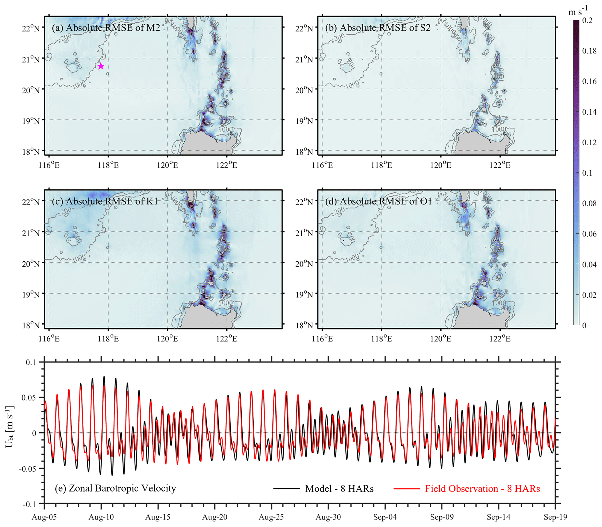
Figure 2 Absolute root-mean-square errors of zonal barotropic velocity (U_bt) between the model (500m_8HARs_BT) and the TPXO8-atlas dataset for M2 (a), S2 (b), K1 (c), and O1 (d). (e) Reconstructed time series of zonal barotropic velocity at station DS (marked as magenta star in Fig. 2a) of Exp. 500m_8HARs_BT (black line) versus measured data (red line) obtained by eight key tidal constituents.

In addition to comparison between this model and the global tide model, we extract the DS station outputs with a high sampling rate for comparison with the in situ observations. To avoid the effects of massive high-frequency motions (i.e. environmental noises) in the observational time series on the barotropic regime, we first do the harmonic analysis for zonal barotropic velocities from 5 August to 19 September, then extract the amplitude and phase of eight key tidal constituents, and restructure the time series (see red line in Fig. 2e). In terms of the model results, we obtain the time series at station DS in the same way (see black line in Fig. 2e). It is worth mentioning that the discrepancy between the eight-harmonic restructured time series and the raw data in the model is small, since the experiment is basically driven by the eight tidal constituents and does not include any affects from the background environment. By comparing the two time series, the model reliability is validated all through the spring and neap tides. Overall, the model presents nice performance in the barotropic regime.

3.2 Comparison with MODIS images

Apart from the model validation in barotropic tides, we then look over the control run (500m_8HARs) in baroclinic (ISWs) regime by comparing the model results with MODIS images. Figure 3a and b both show two successive ISWs (labelled as IW1 and IW2) in the deep basin with a distance of ∼ 120 km. The lengths, curvatures and locations of IW1 and IW2 in the simulation are consistent with those in the MODIS image. However, two other ISWs occurring over the continental slope and shelf are captured in the numerical simulations, but they are not observed on 14 August in the MODIS–Aqua image due to cloud cover (Fig. 3b). Conversely, the cloud disappeared on 15 August, so the MODIS–Terra sensor gives a clear seascape painting of ISWs both in the shallow water (i.e. IW2) and deep water (i.e. IW3 and IW4). Note that IW2 in Fig. 3b and d is the same ISW, which propagates ∼ 250 km within 19 h and 35 min. All ISWs (IW2, IW3 and IW4) in Fig. 3c and d occur at the fairly close locations with analogous wave properties. From the perspective of crest-line lengths, the numerical model shows good agreement with the MODIS images, namely 131 km versus 133 km for IW2 in Fig. 3a and b, 187 km versus 198 km for IW3, and 74 km versus 69 km for IW4 in Fig. 3c and d. Note that the sea surface gradients (|∇η|) larger than 2 cm km⁻¹ along the crest lines are extracted and defined as the crest-line lengths of ISWs. Besides, in the water depth shallower than 500 m, the modelled IW2 exhibits an ISW train with trailing waves, which is also shown in the MODIS image. As the model neglects wind above the sea surface and other marine dynamical processes, there are still some subtle nuances of wave characteristics between them. Overall, this model nicely demonstrates spatial distributions of ISWs in the NSCS, based on the comparison with remote sensing imagery.

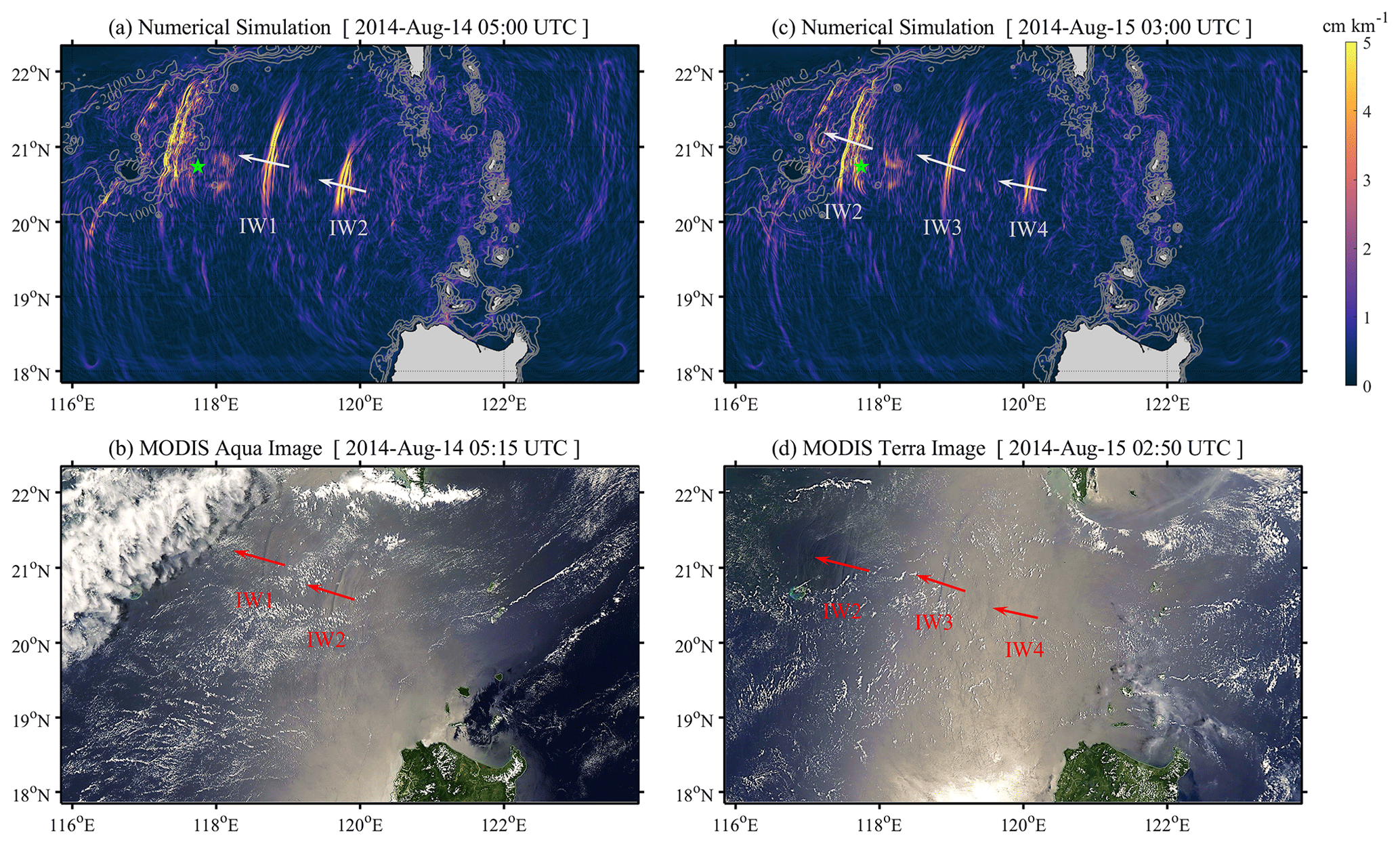
Figure 3 (a) Sea surface height gradients induced by internal solitary waves (ISWs) at 05:00 UTC on 14 August 2014 and (b) MODIS–Aqua image obtained at 05:15 UTC on 14 August 2014. (c) Same as (a) but at 03:00 UTC on 15 August 2014. (d) Same as (b) but for MODIS–Terra at 02:50 UTC on 15 August 2014. Note that the MODIS images in (b) and (d) are freely downloaded from the NASA Worldview application (https://worldview.earthdata.nasa.gov, last access: 17 May 2023, open source).

3.3 Comparison with in situ observations

To further evaluate the model performance in reproducing ISWs, we introduce the in situ observations. The vertical structure and timing of the wave arrivals, after crossing the deep basin, can be seen in details using daily plots (Fig. 4a–g) of the temperature isotherms and baroclinic (ISW-induced) velocities from 8 to 14 August at mooring DS. For clarity, only the results in upper 900 m are shown in Fig. 4, including the main wave-induced temperature fluctuations. On the basis of space–time diagram of isopycnal displacements along the main propagation paths of ISWs (not shown), the averaged nonlinear internal wave speeds are ∼ 3.0 m s⁻¹ from the Luzon Strait to the deep basin, so it takes roughly 1.5 d for ISWs to propagate from the generation site to the targeted station (DS). We move the arrival time (i.e. 00:00 UTC 8 August –00:00 UTC 14 August) of ISWs 1.5 d forward at the station DS, so the related barotropic tides gradually increase during the spring tidal cycle at the Luzon Strait (i.e. 12:00 UTC 6 August–12:00 UTC 12 August). It explains why ISWs were relatively weak and linear from 8 to 10 August (Fig. 4a–c), but they became significant and nonlinear from 11 to 14 August (Fig. 4d–g). A single ISW was captured around 12:00 UTC from 11 to 14 August, which arrived at the location at approximately the same time every day (termed as type-A ISWs by Ramp et al., 2004). Meanwhile, a wave train, consisting of two dominant solitons and some small trailing waves, arrived at the station an hour later each day, showing the same wave characteristics as type-B ISWs in Ramp et al. (2004).

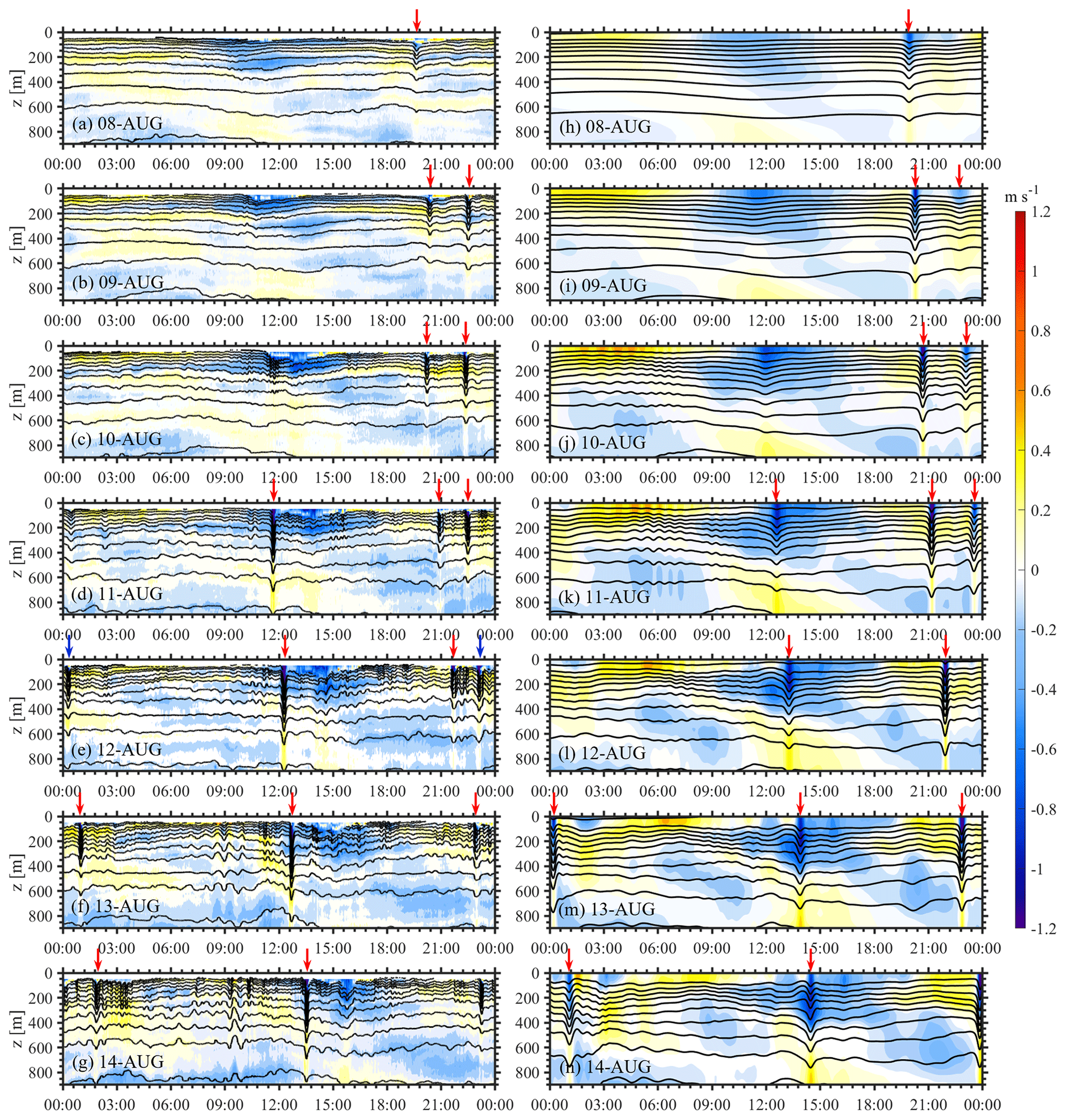
Figure 4 (a–g) Temperature isotherms (contours) and baroclinic velocities (shades) in the wave propagation direction from 8 to 14 August at station DS from in situ observation. (h)–(n) Same as (a)–(g) but for the model (500m_8HARs). Red arrows indicate ISWs that model captured, while blue arrows present the missed ones.

In terms of the model, we also use the daily plots (Fig. 4h–n) at station DS with 1 min sampling rate to show its similarity to the in situ observations. An increasing trend of wave amplitude and nonlinearity is obvious from 8 August to 14 August in the model results, suggesting precise depictions of barotropic tides and ISWs' characteristics. Specifically, both type-A (single solitons) and type-B ISWs (wave trains) are displayed with analogous arrival time, wave-induced (baroclinic) velocity (colour shades in Fig. 4) and wave amplitude (contours in Fig. 4) compared to those in the observations. It's worth noting that even the linear internal tides and/or hydraulic jumps around 12:00 UTC from 8 to 10 August are reproduced. Although the model omits some small wave signals (see blue arrows in Fig. 4e) in the observations, which might be induced by non-tidal processes such as background currents, the model still shows a good performance in the ISW reproduction.

To quantitatively identify the model accuracy, we select 15 ISWs (marked as red arrows in the left column of Fig. 4), extract their wave properties (i.e. arrival time, maximum wave-induced velocity, propagation direction and maximum mode-1 wave amplitude), and compare them between in situ observations and numerical simulations. We obtain wave propagation direction by computing the angle of baroclinic zonal and meridional components in the layer with maximum velocity. The maximum mode-1 wave amplitude (A₁) is extracted from the mooring data and model outputs by least-squares fitting density perturbation profiles ρ^′(z) to normalized modal structure function W_n(z), following the similar procedures to those described by Buijsman et al. (2010a) and Rayson et al. (2012). Although the mode-1 wave amplitude can also be extracted by least squares fitting the horizontal baroclinic velocity, Rayson et al. (2019) suggested that the method in velocity field was fuzzy with unidirectional internal waves. The modal structure function can be resolved by a shear-free Taylor–Goldstein equation with the background stratification N²(z), which is given by

$$\begin{array}{}\text{(2)}& {\displaystyle \frac{d^{\mathrm{2}}{W}_{\mathrm{n}}\left(z\right)}{\mathrm{d}{z}^{\mathrm{2}}}}+{\displaystyle \frac{N^{\mathrm{2}}\left(z\right)}{c_n}}{W}_{\mathrm{n}}\left(z\right)=\mathrm{0},\end{array}$$

with the boundary conditions $W_{\mathrm{n}}\left(\mathrm{0}\right)=W_{\mathrm{n}}\left(-H\right)=\mathrm{0}$. Subscript n represents the mode number and c_n is the phase speed of the linear internal waves in nth mode. The buoyancy perturbation b(z), depending on density perturbation ρ^′(z), is written as

$$\begin{array}{}\text{(3)}& b\left(z\right)=-g{\displaystyle \frac{{\mathit{\rho }}^{\prime }\left(z\right)}{{\mathit{\rho }}_{\mathrm{0}}}},\end{array}$$

in which ρ₀ is the reference density. Following the internal wave polarization relationships (Gerkema and Zimmerman, 2008), we fit the wave amplitudes (A_n) in different vertical modes to b(z) in both in situ observations and numerical simulations via

$$\begin{array}{}\text{(4)}& b\left(z\right)=\sum _{n=\mathrm{1}}^{\mathrm{5}}{A}_{\mathrm{n}}{N}^{\mathrm{2}}\left(z\right)W_{\mathrm{n}}\left(z\right).\end{array}$$

Here, we select the first five vertical modes (n=1–5) to do the least-squares fitting and mainly discuss the mode-1 wave amplitude (A₁) due to its significant dominance (Fig. 4).

According to the above approaches, we extract the four wave properties for 15 ISWs and plot Fig. 5, in which observation and model results are shown in red and green, respectively. First, we list the arrival time of ISWs on the two sides of Fig. 5. The bias between observation and model is always smaller than 1.5 h, and the root mean square deviation (RMSD) is 0.71 h, indicating accurate depiction of ISW arrival time in the control run (500m_8HARs). Second, the maximum baroclinic velocity (Fig. 5a) and the averaged values (0.98 and 1.18 m s⁻¹, respectively) are shown in the solid lines. It is suggested that the model underestimates the baroclinic velocity due to neglect of some background non-tidal signals, thereby introducing a RMSD of 0.41 m s⁻¹. Third, the averaged propagation directions of ISWs are ∼ 285 and ∼ 291^∘, respectively (the angle measured anticlockwise from north) in the model results and observational data with a RMSD of 8.35^∘. It is worth mentioning that the type-A ISWs mainly propagate westward, while the type-B ISWs propagate north-westward in both observation and model, verifying the model's reliability to some extent. Finally, the averaged maximum mode-1 wave amplitude (∼ 108 m) in the model is close to that (∼ 99 m) in the observation. Nonetheless, the RMSD of mode-1 wave amplitude is 37.27 m. Overall, the control run can basically reproduce various wave properties of ISWs observed in the vicinity of the Dongsha Atoll in the NSCS.

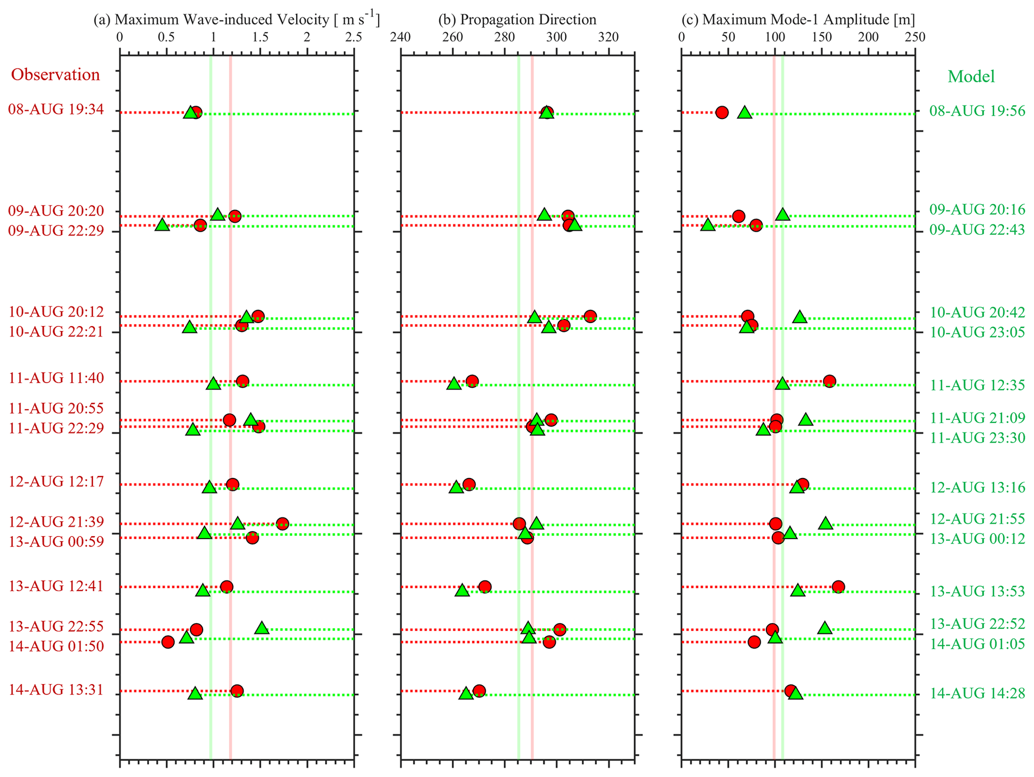
Figure 5 Maximum wave-induced velocities (a), propagation directions (b) and maximum mode-1 wave amplitudes (c) of 15 ISWs at station DS from in situ observations (red circles) and numerical models (green triangles). Averaged values are shown by solid lines.

4 Assessment of factors affecting 3D model forecasting precision

In this section, based on the control run, we alter the model configurations, such as the requirements of horizontal resolutions, numbers of tidal constituents and initial stratification, to respectively estimate their effects on the model forecasting precision of ISWs in the NSCS.

To determine the roles of model horizontal resolutions, tidal constituents and initial stratification in reproducing ISWs in the NSCS, a set of 3D sensitivity numerical simulations are employed with different configurations, which are listed in Table 2. Details in configuration changes are as follows.

1. Exps. 3 and 4 (250m_8HARs and 1000m_8HARs). Compared to 500m_8HARs, the horizontal resolution (Δx) is set as 250 and 1000 m in both zonal and meridional directions, respectively.

2. Exps. 5–7 (500m_1HAR, 500m_4HARs, and 500m_13HARs). Compared to 500m_8HARs, the sensitivity experiments are driven by a single tidal constituent (M2), four main tidal constituents (M2, S2, K1 and O1), and 13 tidal constituents (M2, S2, N2, K2, K1, O1, P1, Q1, M4, MS4, MN4, MM and MF), respectively.

3. Exp. 8 (500m_Real_N2). A real stratification profile of background temperature at the mooring station DS is imposed as the initial condition, which is derived from the in situ measurements. A backward-in-time low-pass filter derived from a finite impulse response differential equation is used to compute the background temperature (Rayson et al., 2019).

   $$\begin{array}{}\text{(5)}& {\displaystyle \frac{\mathrm{d}\stackrel{\mathrm{‾}}{T}}{\mathrm{d}t}}={\displaystyle \frac{\mathrm{1}}{{\mathit{\tau }}_{\mathrm{f}}}}\left(T-\stackrel{\mathrm{‾}}{T}\right),\end{array}$$

   in which τ_f is the filtering timescale, set to 35 h, corresponding to the local Coriolis frequency. T and $\stackrel{\mathrm{‾}}{T}$ are the instantaneous and background temperature, respectively. Then, the background temperature at each observational time step i is given as

   $$\begin{array}{}\text{(6)}& {\stackrel{\mathrm{‾}}{T}}^{i+\mathrm{1}}={\stackrel{\mathrm{‾}}{T}}^i+{\displaystyle \frac{\mathrm{\Delta }t}{{\mathit{\tau }}_{\mathrm{f}}}}(T^{i+\mathrm{1}}-{\stackrel{\mathrm{‾}}{T}}^i),\end{array}$$

   where Δt is the sampling rate (10 s for the temperature and CTD sensors, 15 s for the CT sensors). The background temperature profile is ultimately obtained by low-pass filtering at each layer (see red line in Fig. 1b).

Table 2 Summary of all experimental configurations.

4.1 Requirements of resolutions

Various 3D models with different resolutions were implemented to simulate ISWs in the NSCS in previous studies (e.g. Vlasenko et al., 2010; Zhang et al., 2011; Lai et al., 2019). However, which resolution is adequate to satisfy the ISW prediction precision and save computational resources to the utmost in the meantime has yet to be discussed. Here, we run two sensitivity experiments (Exps. 250m_8HARs and 1000m_8HARs) with horizonal resolutions of 250 and 1000 m, to respectively compare the model performance in different aspects with the control run (resolution of 500 m).

First, the spatial distributions of ISWs are exhibited via the snapshots of sea surface height gradients (|∇η|) at 12:00 UTC on 12 August 2014. In the control run (500m_8HARs), three ISWs (labelled as IWB1, IWA1, and IWB2 from west to east) with distinct crest lines successively occur between 116 and 120^∘ E (see Fig. 6a), in which IWB1 and IWB2 are internal wave packets with trailing waves (type-B wave) and IWA1 is a single soliton (type-A wave). As IWB1 approaches the continental slope and shelf, the leading wave front fully steepens with a narrow characteristic half-width, suggesting its strong nonlinearity. IWB2 also shows up as a wave packet with many secondary waves in the developing stage, although its nonlinearity is slightly weaker than IWB1's. Conversely, the single soliton IWA1 with relatively long crest line and broad characteristic half-width is about to pass mooring station DS (marked as green star in Fig. 6). In comparison, the Exps. 250m_8HARs and 1000m_8HARs reproduce these three waves as well, but with some subtle discrepancies between them. In Exp. 250m_8HARs, more details of wave properties are clarified (Fig. 6b). Specifically, the secondary waves of IWB1 and IWB2 are more visible than those in 500m_8HARs. However, in Exp. 1000m_8HARs, some fine structures of ISWs are not well resolved. For instance, only one secondary wave is found behind the leading wave of IWB2, and the south portion of IWA1 crest line is barely observed (Fig. 6c).

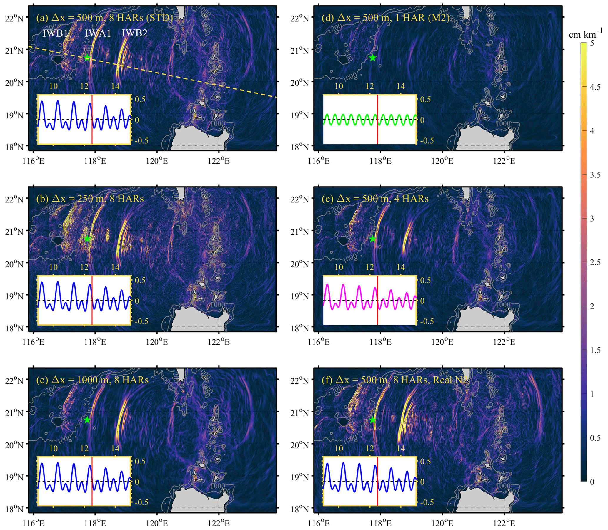
Figure 6 Sea surface height gradients at 12:00 UTC on 12 August 2014 in the model (a) 500m_8HARs, (b) 250m_8HARs, (c) 1000m_8HARs, (d) 500m_1HAR, (e) 500m_4HARs and (f) 500m_Real_N2. Note that the dashed line in (a) is the selected transect to present vertical structure of ISWs. Small panels on the bottom left indicate the zonal barotropic velocity (unit in m s⁻¹) in the Luzon Strait with the solid lines showing the tidal conditions at the selected time.

Then, we select a transect along the main propagation path of ISWs (shown in dashed line in Fig. 6a) at 12:00 UTC on 12 August 2014 to compare the vertical structure of ISWs among three experiments (see Fig. 7). In Fig. 7, blue (yellow) colour shades represent westward (eastward) baroclinic velocity and contours are temperature isotherms. Linear internal waves, such as internal wave beams near the generation site (120–121^∘ E), are nicely reproduced in all numerical experiments. Nonetheless, nonlinear internal waves present different wave characteristics in different cases. In Exp. 500m_8HARs, the single soliton IWA1 and the wave packet IWB2 with a series of trailing waves are apparent in the slice, but IWB1 is not included (Fig. 7a). In Exp. 250m_8HARs, IWA1 and IWB2 occur at the same location as those in Exp. 500m_8HARs. IWA1 show similar properties in two cases, but the secondary waves of IWB2 are better described in Exp. 250m_8HARs. By comparison, IWA1 shows its weak nonlinearity with small vertical displacement and broad characteristic half-width (i.e. horizontal distance between the wave front and wave trough) in Exp. 1000m_8HARs. Besides, only one secondary wave appears in the IWB2 packet in Exp. 1000m_8HARs.

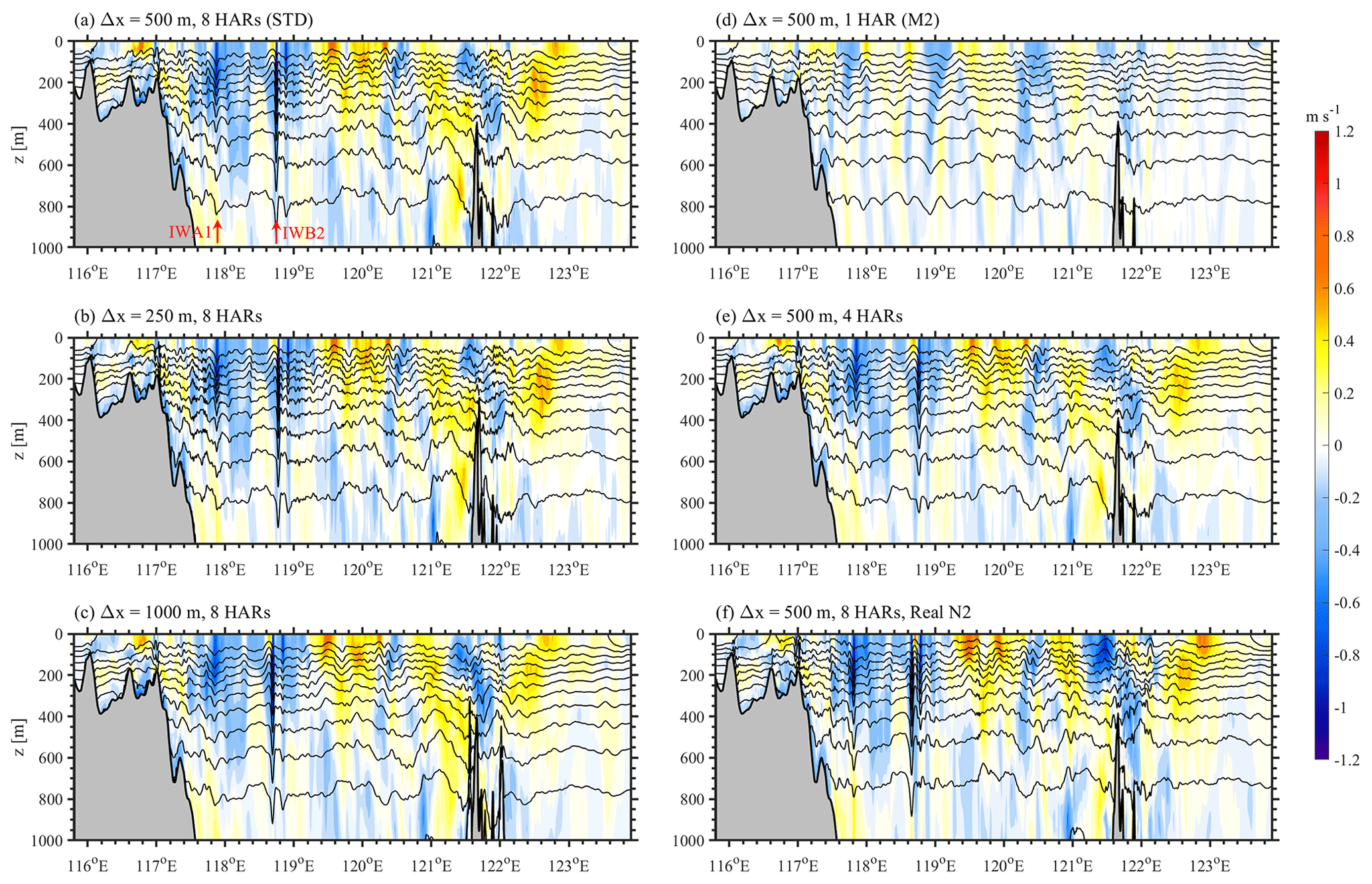
Figure 7 Temperature isotherms (contours) and baroclinic velocities (shades) along the transect (dashed line in Fig. 6a) at 12:00 UTC on 12 August 2014 in the model (a) 500m_8HARs, (b) 250m_8HARs, (c) 1000m_8HARs, (d) 500m_1HAR, (e) 500m_4HARs and (f) 500m_Real_N2. Note that waves IWA1 and IWB2 are labelled in (a) with red arrows.

Last, a two-day time segment of observational temperature and baroclinic velocities from 18:00 UTC on 11 August to 18:00 UTC on 13 August 2014 at the station DS is extracted to demonstrate the sensitivity model capability of simulating vertical structures of ISWs over the continental slope (Fig. 8). In the control run (500m_8HARs, Fig. 8b), two wave packets and two single solitons successively arrive at the station, keeping the consistency with the observation, although their characteristic half-widths are slightly broader than those in the field measurements (Fig. 8a). Meanwhile, some small fluctuations, occurring in the observations, are not included in the control run. In Exp. 250m_8HARs (Fig. 8c), the half-widths are narrower than those in the Exp. 500m_8HARs, which agree better with the real internal wave field. Besides, more fluctuations, i.e. those small wave signals (09:00 UTC on 12 August and 09:00 UTC on 13 August) in front of the single solitons, are reproduced in this experiment. Conversely, in Exp. 1000m_8HARs, internal wave trains can still be reproduced with relatively weak nonlinearity, but the single solitons are not correct due to their tiny amplitudes and linear wave structures.

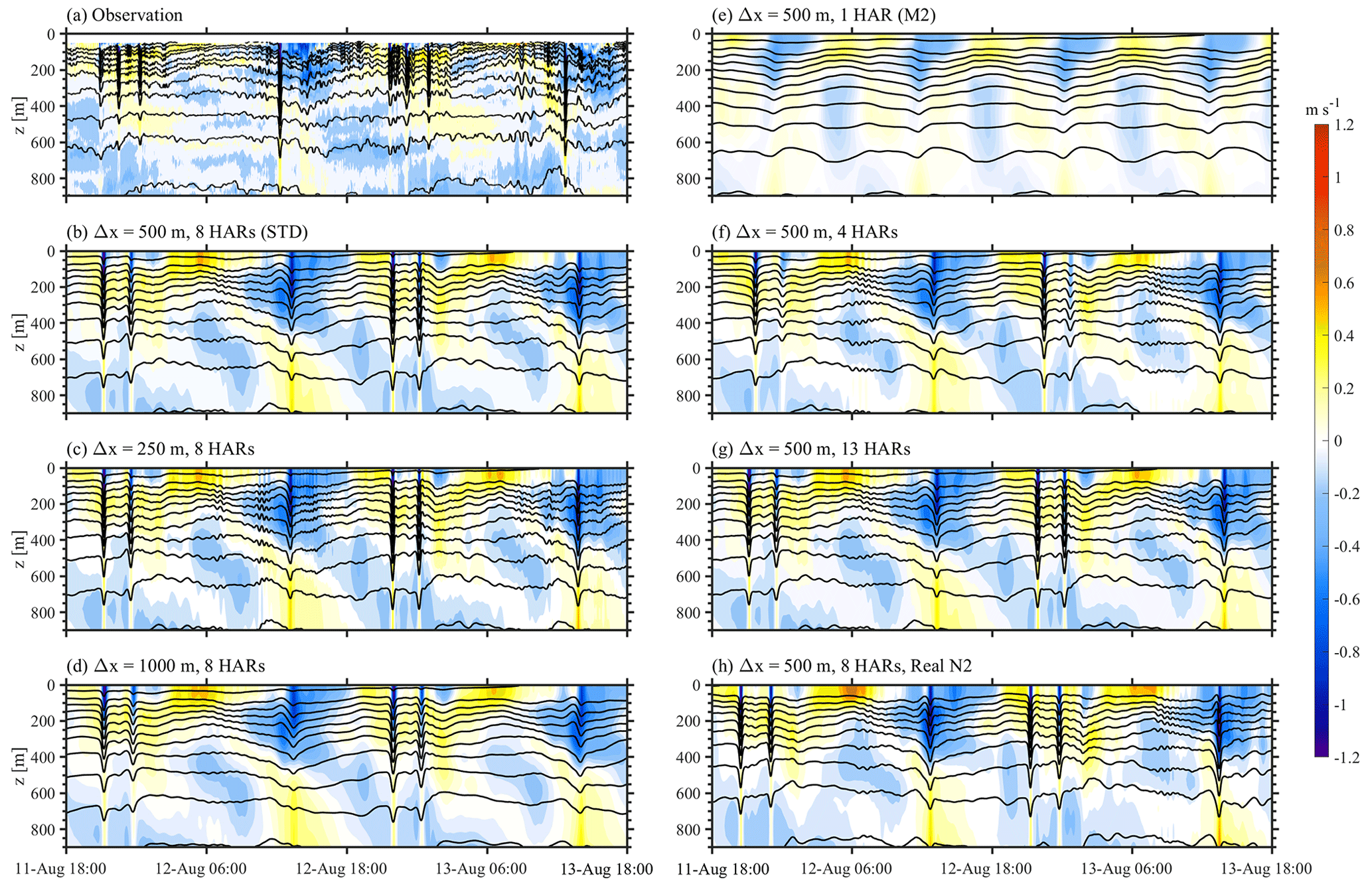
Figure 8 Time series of temperature isotherms (contours) and baroclinic velocities (shades) at station DS from 18:00 UTC on 11 August to 18:00 UTC on 13 August 2014 in the observation (a) and in the model (b) 500m_8HARs, (c) 250m_8HARs, (d) 1000m_8HARs, (e) 500m_1HAR, (f) 500m_4HARs, (g) 500m_13HARs and (h) 500m_Real_N2.

To quantitatively evaluate the model performance of sensitivity experiments, we present the bias of five wave properties of 15 ISWs (marked as red arrows in Fig. 4) between model results and observational data in Fig. 9. The biases of arrival time are generally smaller than 1 h (see black and blue circles in Fig. 9a) for Exps. 500m_8HARs and 250m_8HARs, whose RMSDs are 0.71 and 0.67 h, respectively. In contrast, the bias for Exp. 1000m_8HARs is larger than 1 h (red circles in Fig. 9a) and its RMSD is 0.79 h. In terms of the wave-induced velocity (Fig. 9b), the RMSDs are 0.38, 0.41 and 0.48 m s⁻¹ in Exps. 250m_8HARs, 500m_8HARs and 1000m_8HARs, respectively. The RMSDs of propagation directions are very close (∼ 8.5^∘) in the three experiments (see Table 3). As for the mode-1 wave amplitudes, Exps. 250m_8HARs and 500m_8HARs overestimate the wave amplitudes in most cases (see positive biases in Fig. 9d), thereby resulting in RMSDs of 38.12 and 37.27 m, respectively. Conversely, Exp. 1000m_8HARs would underestimate the wave amplitudes of majority ISWs with dominant negative biases in Fig. 9d, resulting in a RMSD of 40.28 m (Table 3). Last but not least, Exps. 500m_8HARs and 1000m_8HARs inaccurately depict characteristic half-widths of ISWs with RMSDs of 1.07 and 2.41 km, while Exp. 250m_8HARs performs well with a RMSD of 0.64 km (Fig. 9e). The relative difference of RMSD suggests that Exp. 250m_8HARs increases to 40 % accuracy of predicting characteristic half-widths by comparing Exp. 500m_8HARs. From the perspective of computational resources, Exps. 250m_8HARs, 500m_8HARs and 1000m_8HARs spend 20.4×10⁴ CPU hours, 4.6×10⁴ CPU hours and 1.0×10⁴ CPU hours, respectively.

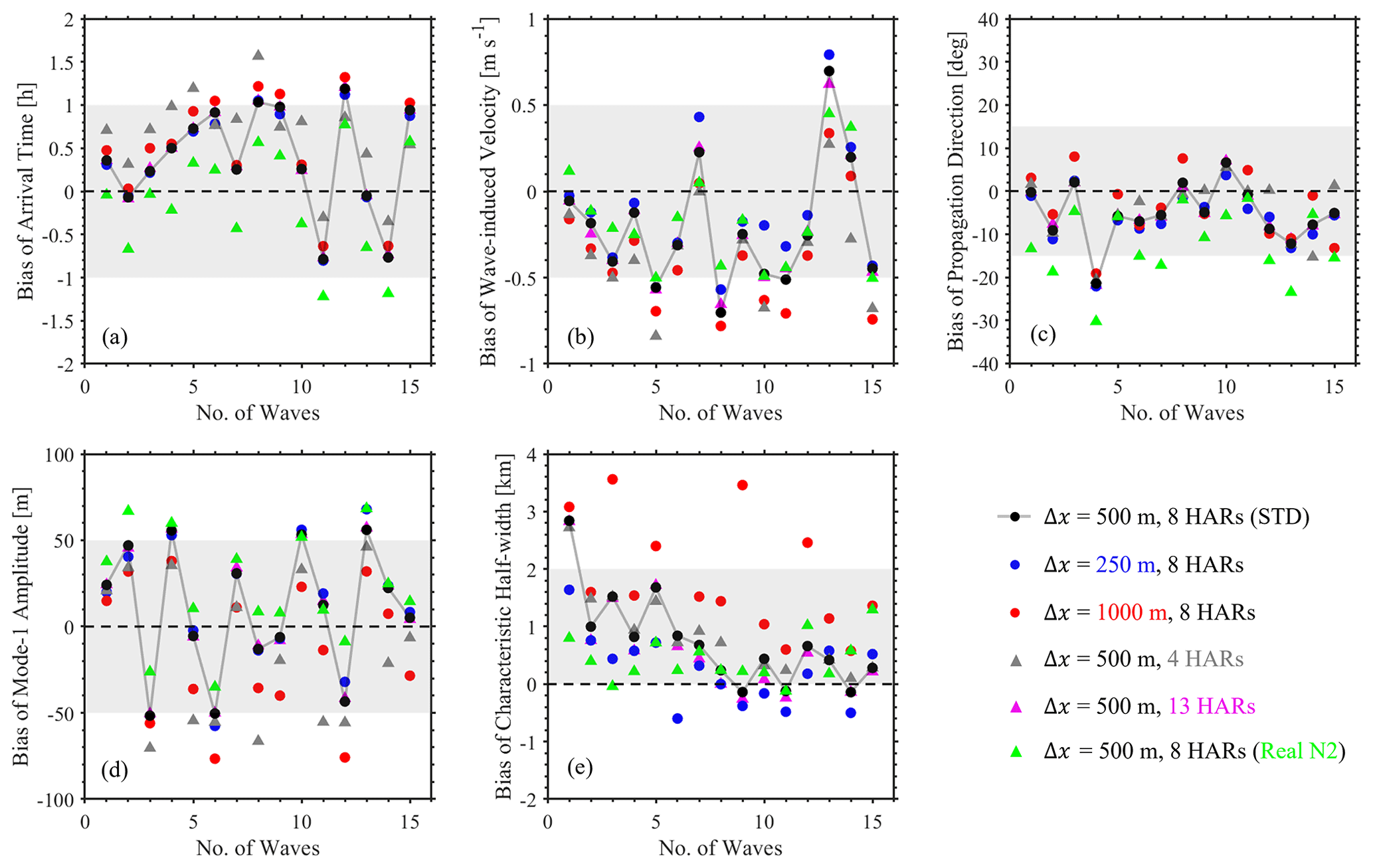
Figure 9 Bias of arrival time (a), maximum wave-induced velocities (b), propagation directions (c), maximum mode-1 wave amplitudes (d) and characteristic half-widths (e) for 15 ISWs at station DS. Colours present different experiments.

Table 3 Root mean square deviation (RMSD) of wave properties between field observation and 3D sensitivity simulations at the mooring station in the vicinity of the Dongsha Atoll.

In summary, the control run with a resolution of 500 m can basically reproduce the principal ISW field in the NSCS, while the sensitivity model with a higher resolution of 250 m would be a better solution to identify wave properties, in particular of the wave nonlinearity. Nonetheless, a 250 m resolution model spends nearly a 5-fold computational resources of a 500 m resolution model in the same model domain. Besides, the model with a lower resolution of 1000 m underestimates the nonlinearity of ISWs, thereby resulting in an inaccurate ISW field in the NSCS.

4.2 Requirements of tidal constituents

The 3D/2D models with different numbers of barotropic tidal constituents (e.g. single harmonic, four harmonics and eight harmonics) were commonly imposed to investigate the generation mechanisms of ISWs in the NSCS in previous studies (e.g. Li, 2014; Buijsman et al., 2010a; Jin et al., 2021). However, whether a single tidal constituent can satisfy the reproduction of a real ISW field and how many tidal constituents are required for a realistic ISW model are still questions. Here, we run three sensitivity experiments (Exps. 500m_1HAR, 500m_4HARs and 500m_13HARs) with different numbers of tidal harmonics to answer the questions by comparing the model performance with the control run (500m_8HARs).

We first discuss the model requirements of tidal constituents from the point of view of the ISW horizontal distributions and look back to Fig. 6. Note that time series of zonal barotropic currents at the generation site (Luzon Strait) are presented at the bottom left for each panel, where single, four and eight tidal constituent(s) are shown in green, magenta and blue, respectively. By comparing Exp. 500m_1HAR (Fig. 6d) and 500m_8HARs (Fig. 6a), we find that the single M2 tidal harmonic is not adequate to reproduce ISWs in the NSCS, so only some linear internal tides are detected on the sea surface via |∇η|. In contrast, Exp. 500m_4HARs (Fig. 6e) nearly recreates the analogous scenario of ISWs to Exp. 500m_8HARs, where IWB1, IWA1 and IWB2 appear at the same locations. Nonetheless, the crest-line length (∼ 134 km) of IWB2 in Exp. 500m_4HARs is slightly shorter than that (∼ 167 km) in Exp. 500m_8HARs, and the secondary waves of IWB2 are unclear in Exp. 500m_4HARs (see Fig. 6e). |∇η| in Exp. 500m_13HARs are not presented in Fig. 6, since it shows the exact same spatial patterns of ISWs as those in Exp. 500m_8HARs, suggesting the principle eight tidal constituents are fine enough to satisfy accurate reproduction of the horizontal features of ISWs in a realistic oceanic model.

We then consider the difference of ISW vertical structures in sensitivity experiments with various tidal forcing via the selected transect and mooring station DS. In Exp. 500m_1HAR, only linear internal waves are captured from the generation site to the slope, suggesting that single M2 tidal constituent without amplification factors can only contribute to internal tides and linear internal wave beams in NSCS (see Figs. 7d and 8e). Unless the magnitudes of M2 barotropic tides are amplified, ISWs are likely to be generated (e.g. Yuan et al., 2020). In Exp. 500m_4HARs (Figs. 7e and 8f), the single soliton IWA1 is reproduced with a smaller amplitude and weaker nonlinearity than that in Exp. 500m_8HARs. Besides, the secondary waves of IWB2 are barely observed in Exp. 500m_4HARs, which are much clearer in Exp. 500m_8HARs (Figs. 7a and 8a). Figure 8a and g depict the striking similarity of wave characteristics between Exp. 500m_8HARs and Exp. 500m_13HARs.

Last, we quantitatively estimate the sensitivity model capability of reproducing ISWs, by computing the biases and RMSDs of five wave properties (see Fig. 9 and Table 3) in the cases with different tidal forcing. Since Exp. 500m_1HAR cannot predict ISWs with significant amplitudes, we exclude it in the following analysis. In terms of Exp. 500m_13HARs with 13 tidal constituents, the biases and RMSDs of five wave properties are very close to those in the control run with eight harmonics (see overlapped black circles and magenta triangles in Fig. 9 and Table 3). Conversely, Exp. 500m_4HARs shows significant difference in the biases and RMSDs of five wave properties from the control run. Specifically, in Fig. 9a, the RMSD of arrival time (0.81 h) is larger in Exp. 500m_4HARs than that in Exp. 500m_8HARs (0.71 h). In addition, Exp. 500m_4HARs underestimates averaged wave-induced velocity for about 38 % and averaged mode-1 wave amplitude for about 15 %, which result in large negative values of biases (see magenta triangles in Fig. 9b and c), corresponding to 0.58 m s⁻¹ and 43.69 m of RMSDs, respectively. In terms of the characteristic half-widths, Exps. 500m_4HARs and 500m_13HARs with RMSDs of 1.10 and 1.01 km show analogous performance to the control run Exp. 500m_8HARs with a RMSD of 1.07 km.

In summary, the model with 8 (or 13) primary tidal constituents can accurately reproduce the real ISW field in the NSCS, while the sensitivity model with four key harmonics (M2, S2, K1 and O1) would underestimate the magnitudes of some secondary wave within a wave packet. In addition, the model only driven by M2 tide can only characterize wave properties of linear internal waves (tides) instead of ISWs.

4.3 Initial stratification selections

As ISWs generate via tide-topography interaction in the stratified water, the stratification selection is crucial to directly affect the model capabilities. Here, we extract the background stratification from the in situ measurements at mooring station DS as the initial condition to run the sensitivity experiment 500m_Real_N2, and we compare the model results with the control run (500m_8HARs) with a climatological stratification from the WOA18 dataset.

In the model results, the spatial distribution of |∇η| in Exp. 500m_Real_N2 shows an analogous pattern of ISWs to that in Exp. 500m_8HARs. Specifically, three ISWs (i.e. IWB1, IWA1, and IWB2) appear at the same location in the two experiments with similar horizontal wave characteristics (Fig. 6a and f). The visible difference is that the crest line length of the secondary wave of IWB2 is longer with a stronger nonlinearity in Exp. 500m_Real_N2. We then look over the difference of ISW vertical structures between two cases from the perspective of x–z plane along the transect (Fig. 7a and f) and time series at station DS (Fig. 8a and h). It is clearly shown that Exp. 500m_Real_N2 with the real stratification can better characterize the nonlinearity of the single soliton IWA1 and the secondary wave of wave train IWB2. Besides, the comparison with field measurements reveals that Exp. 500m_Real_N2 shows a better precision (13 %) in predicting the arrival time (i.e. RMSD of 0.62 h) of ISWs than the control run (i.e. RMSD of 0.71 h) with the climatological stratification. However, the RMSD of the propagation direction of ISWs is larger in the realistic-stratification case (14.74^∘) than that of the control run (8.35^∘). Last, Exp. 500m_Real_N2 nicely describes the characteristic half-widths of ISWs (RMSD of 0.58 km), which improves 46 % accuracy by comparing that in Exp. 500m_8HARs (RMSD of 1.07 km). To sum up, although the model with climatological stratification works well, applying the real background stratification as the model initial condition would improve the model performance in predicting some wave properties, including arrival time, wave-induced velocity, wave amplitude and characteristic half-width.

5 Discussion and conclusions

Although the 3D realistic model, particularly in Exp. 250m_8HARs, has accurately reproduced the ISW features in the NSCS to some extent, the depictions of soliton numbers within an internal wave packet and propagation direction still have space for improvement. That is, at least three following factors might be considered in the future modelling.

The first factor that may affect the model accuracy is background currents. Here, we download the global Hybrid Coordinate Ocean Model (HYCOM) dataset from 2014 and calculate the background current field by averaging from 5 to 20 August, namely predicting time of the model (see Fig. 10a). In Fig. 10a, there is a clear anticlockwise circulation/eddy pattern on the west side of the Luzon Strait. Xie et al. (2015) suggested that wave properties of ISWs can be significantly influenced by an isolated mesoscale eddy, regardless of a cyclonic or anticyclonic eddy, during the propagation of ISWs. When an ISW passes over a cyclonic eddy, as in Fig. 10a, the crest line will be distorted, thereby modulating the oblique propagation direction of wave to some extent (Xie et al., 2016). In addition, a series of secondary trailing waves are able to form behind the leading wave in the energy-focusing region. Therefore, background currents are supposed to be considered in the future forecasting model, which shows potential improvement in the depiction of soliton numbers within an ISW packet and propagation direction in the NSCS.

Figure 10 (a) Background currents near the sea surface (averaged from 5 to 20 August 2014, derived from the global HYCOM dataset). (b) Background buoyancy frequency at a water depth of 50 m. (c) Time-averaged wind stress at 10 m above the sea surface, which is derived from NCEPv2 hourly dataset.

The second factor is inhomogeneous spatial distribution of stratification. In the current forecasting model, we apply horizontally homogeneous temperature and salinity profiles (Fig. 1d) with the maximum buoyancy frequency of ∼ 0.02 s⁻¹ at a water depth of 50 m. Actually, we also implement a sensitivity experiment (Exp. 3D-TS) with weak spatially varying initial conditions derived from the WOA18 climatology dataset. By comparing experiments 3D-TS and 800m_HARs, it is concluded that the weak spatially varying initial conditions show similar performance in predicting the arrival time and horizontal distributions (Fig. C1), wave amplitudes and wave-induced velocities (Fig. C2) of ISWs to the horizontally homogeneous initial conditions. However, the model results would be different with strong spatially varying stratification derived from the ocean reanalysis dataset with a high resolution and sampling rate (e.g. global HYCOM dataset). Since wave speeds of ISWs and internal tides are closely related to vertical structure of stratification based on eigenfunction, the inhomogeneous stratification pattern is likely to affect ISW propagation speed and then modulate their arrival time. Most of previous numerical studies (e.g. Zhang et al., 2011; Alford et al., 2015; Zeng et al., 2019) rarely considered the impacts of horizontally inhomogeneous stratification, but Lai et al. (2019) applied spatially varying stratification in 3D models and indicated that inhomogeneous stratification can achieve better model results to some extent. However, only considering spatially varying temperature and salinity profiles with large values of horizontal gradients (e.g. HYCOM dataset in Fig. 10b) as the initial conditions might lead to spurious geostrophic currents, thereby significantly affecting the true wave field. Hence, spatially varying stratification is worthwhile to be considered together with background currents in future numerical studies in the NSCS.

The last element is external (wind) forcing. As is well known, ISWs are a ubiquitous phenomenon with maximum amplitudes in the ocean interior. Nonetheless, the thermoclines usually occur in the upper layers (shallower than 500 m) in the SCS, which can be significantly affected by extreme wind events (i.e. tropical cyclones; Zhang, 2022). So far, wind forcing has been rarely applied in the numerical modelling of ISWs, except by Lai et al. (2019). As both the ISWs and tropical cyclones are active and frequent in August, September and October in the SCS, the impacts of tropical cyclones on the upper layers should be considered in future numerical simulations, although tropical cyclones did not happen during our predicting period (see Fig. 10c).

In summary, this study introduces a robust ISW forecasting model by comparison with in situ observational data and remote-sensing images, and it quantitatively evaluates the requirements of different factors, including the horizontal resolutions, tidal constituents and initial stratification, to accurately characterize the ISW field with applications to the NSCS. The major findings are listed as follows.

1. A model with a 500 m resolution can basically reproduce the principal ISW field, while a model with a higher resolution of 250 m would be a better solution to identify wave properties but spends nearly 5-fold computational resources of a 500 m resolution case with the same model domain.

2. At least eight primary tidal constituents should be included in the boundary forcing.

3. Compared to climatological stratification, applying the observational background stratification could improve the model performance in predicting some wave properties, namely a 13 % improvement of arrival time and a 46 % improvement of characteristic half-width.

Appendix A: Feasibility study of 2D slice model

Differing from the 3D models, 2D slice models are fairly economical from the perspective of computational resources. In the past few decades, 2D slice models with idealized topography (double ridges) were commonly conducted to investigate ISW dynamics in the NSCS, in particular for the generation mechanisms and the affecting factors of ISWs (i.e. Cai et al., 2002; Shaw et al., 2009; Li, 2014). Here, we attempt to test the 2D model performance along different transects and clarify whether a 2D slice model can be a substitute for a 3D model in the aspect of reproducing a real ISW field in the NSCS.

Three parallel transects with a distance of 0.05^∘ are selected along the main propagation direction of ISWs (see dashed lines in Fig. 1a), which are labelled 2D_500m_8HARs, 2D_500m_8HARs_005N and 2D_500m_8HARs_005S. Δx and Δt are still set as 500 m and 10 s, respectively. Initial conditions and dissipation coefficients are set the same as those in the 3D control run (500m_8HARs). The 2D slice models are also driven by the barotropic tides of eight tidal constituents at both the west boundary (115.8^∘ E, 21.1^∘ N ±0.05^∘) and east boundary (123.8^∘ E, 19.5^∘ N ±0.05^∘). As the transects are not strictly zonal (angle θ=11.2^∘; see Fig. 1a), it is necessary to extract the amplitude (U^′) and phase (ϕ^′) for each harmonic (ω) in the transect direction from the TPXO8-atlas dataset (i.e. U, V, ϕ_U and ϕ_V), given by

$$\begin{array}{}\text{(A1)}& {\displaystyle }{U}^{\prime }=\sqrt{\begin{array}{c}{\left(U\cdot \cos {\mathit{\varphi }}_U\cos \mathit{\theta }-V\cdot \cos {\mathit{\varphi }}_V\sin \mathit{\theta }\right)}^{\mathrm{2}}\\ +{\left(U\cdot \sin {\mathit{\varphi }}_U\cos \mathit{\theta }-V\cdot \sin {\mathit{\varphi }}_V\sin \mathit{\theta }\right)}^{\mathrm{2}}\end{array}},\text{(A2)}& {\displaystyle }{\mathit{\varphi }}^{\prime }=\arctan \left({\displaystyle \frac{U\cdot \sin {\mathit{\varphi }}_U\cos \mathit{\theta }-V\cdot \sin {\mathit{\varphi }}_V\sin \mathit{\theta }}{U\cdot \cos {\mathit{\varphi }}_U\cos \mathit{\theta }-V\cdot \cos {\mathit{\varphi }}_V\sin \mathit{\theta }}}\right).\end{array}$$

Here, we apply the standard 2D experiment along the selected transect (see the black dashed line in Fig. 1a) and label it 2D_500m_8HARs. The model is driven by eight principle tidal constituents on the both lateral boundaries, which are extracted from the TPXO8 dataset (following Eqs. A1 and A2). Note that initial conditions and other model configurations in Exp. 2D_500m_8HARs are the same as those in the 3D control run (500m_8HARs). In addition, we run two sensitivity experiments (Exps. 2D_500m_8HARs_005N and 2D_500m_8HARs_005S) along the two parallel transects (see red dashed lines in Fig. 1b).

In the 2D standard case (2D_500m_8HARs), ISWs subsequently generate in the double ridge, then propagate westward, and eventually arrive at the station in the form of wave trains (Fig. A1b). The wave amplitudes are greater than those in the 3D control run (Fig. A1a). At the station outputs (Fig. A1f), we find that Exp. 2D_500m_8HARs can only reproduce ISW packets, but it cannot discriminate type-A and type-B ISWs. Although the occurrence frequency of ISWs is also twice per day in Exp. 2D_500m_8HARs, the arrival time of those ISW packets is not consistent with that in Exp. 500m_8HARs (Fig. A1e) and in the field measurements (Fig. 8a). In Exp. 2D_500m_8HARs_005N, ISWs are rarely found along the transect (Fig. A1c), likely due to the relatively gentle topography and small tidal forcing at the lateral boundaries. At the station outputs (Fig. A1g), only small temperature fluctuations are captured. Conversely, Exp. 2D_500m_8HARs_005S shows analogous wave fields to Exp. 2D_500m_8HARs (Fig. A1d). Specifically, ISW packets with a half-day cycle are dominant, but their arrival times are postponed for about 2 h (Fig. A1h).

To sum up, 2D slice models along different transects (even 0.05^∘ apart) present totally different ISW characteristics, which are inconsistent with the 3D model results and in situ measurements. Therefore, the 3D model is the best and sole option to correctly reproduce the ISW field in the real ocean, while the 2D model is more suitable for the mechanism investigations.

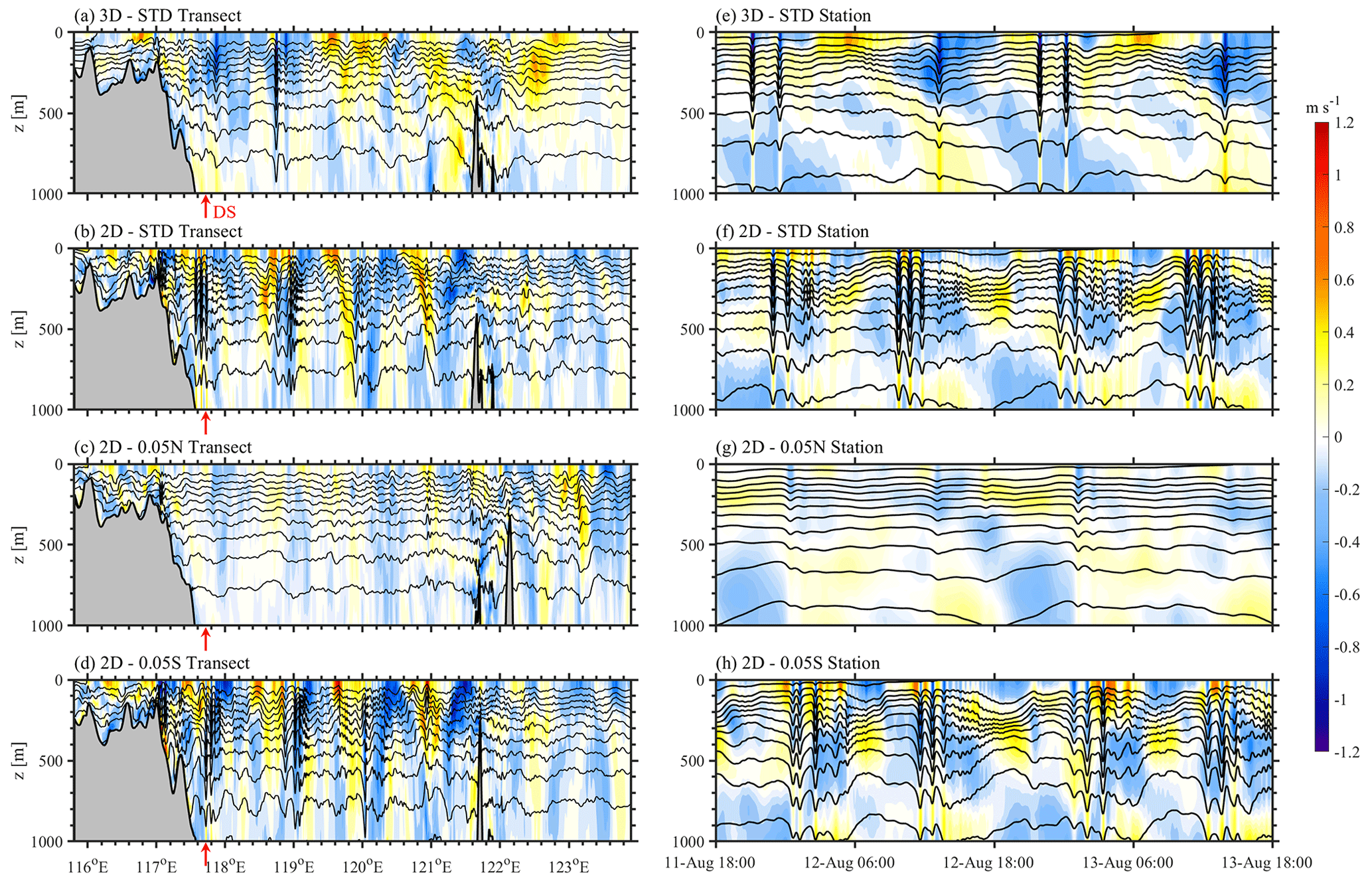
Figure A1 Temperature isotherms (contours) and baroclinic velocities (shades) along the transect at 12:00 UTC on 12 August 2014 in the 3D model (a) 500m_8HARs, in the 2D model (b) 2D_500m_8HARs, (c) 2D_500m_8HARs_005N and (d) 2D_500m_8HARs_005S. (e–h) Corresponding time series at the stations, which are marked as red arrows in (a–d).

Appendix B: Quasi-steady state of the model

Due to the limitation of the computational resources, we admit that the model-integrated time (3 d) might be relatively short for the model spin-up. When we calculate the averaged baroclinic kinetic energy (KE_bc) in the inner model domain (Fig. B1), it is found that the depth-integrated KE_bc keeps increasing in the first 7 d (see red line in Fig. B1a), which is related to the flooding barotropic tides (see Fig. B1b). Actually, ${\int }_{-H}^{\mathrm{0}}{\mathrm{KE}}_{\mathrm{bc}}\mathrm{d}z$ reaches 10 kJ m⁻² on the 3rd model day, whose magnitude is equivalent to that during the neap tides (i.e. 12th to 15th model day). It demonstrates that the 3D model reaches a quasi-steady state after 3 d. Moreover, the comparison between the model results and field observations at the mooring station DS verifies the model accuracy from 8 August (the third model day) as well. Therefore, first 3 d is considered as the spin-up time in this work.

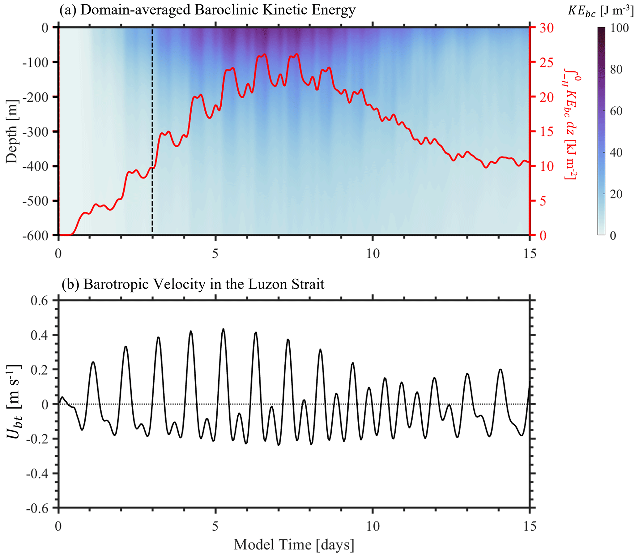
Figure B1 (a) Domain-averaged baroclinic kinetic energy (KE_bc, in units of J m⁻³) in the inner model domain. Note that the red solid line is domain-averaged, depth-integrated KE_bc (${\int }_{-H}^{\mathrm{0}}{\mathrm{KE}}_{\mathrm{bc}}\mathrm{d}z$, in units of kJ m⁻²). (b) Time series of barotropic velocity in the Luzon Strait.

Appendix C: Figures of experiments 3D-TS and 500m_8HARs

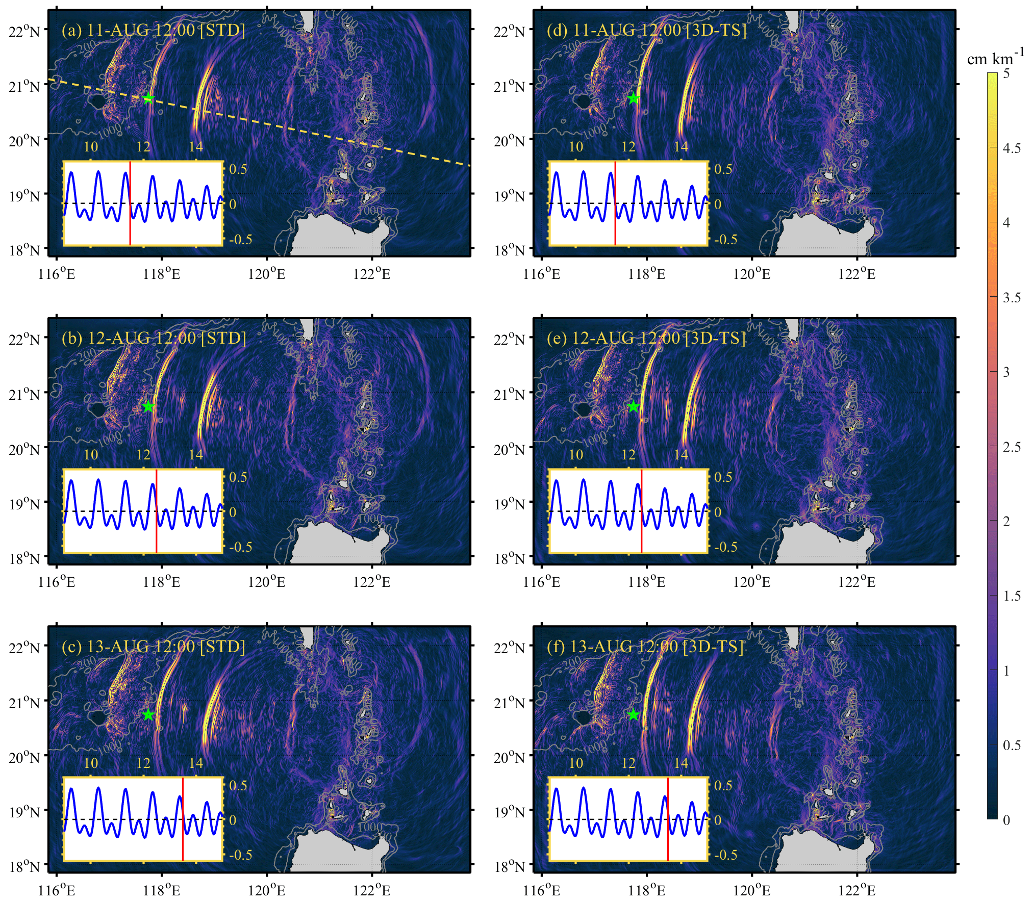
Figure C1 (a–c) Snapshots of sea surface gradients (|∇η|) at 12:00 UTC on 11, 12 and 13 August in the standard experiment (Exp. 500m_8HARs), respectively. (d)–(f) Same as (a)–(c) but in the sensitivity experiment with horizontally inhomogeneous temperature and salinity (Exp. 3D-TS).

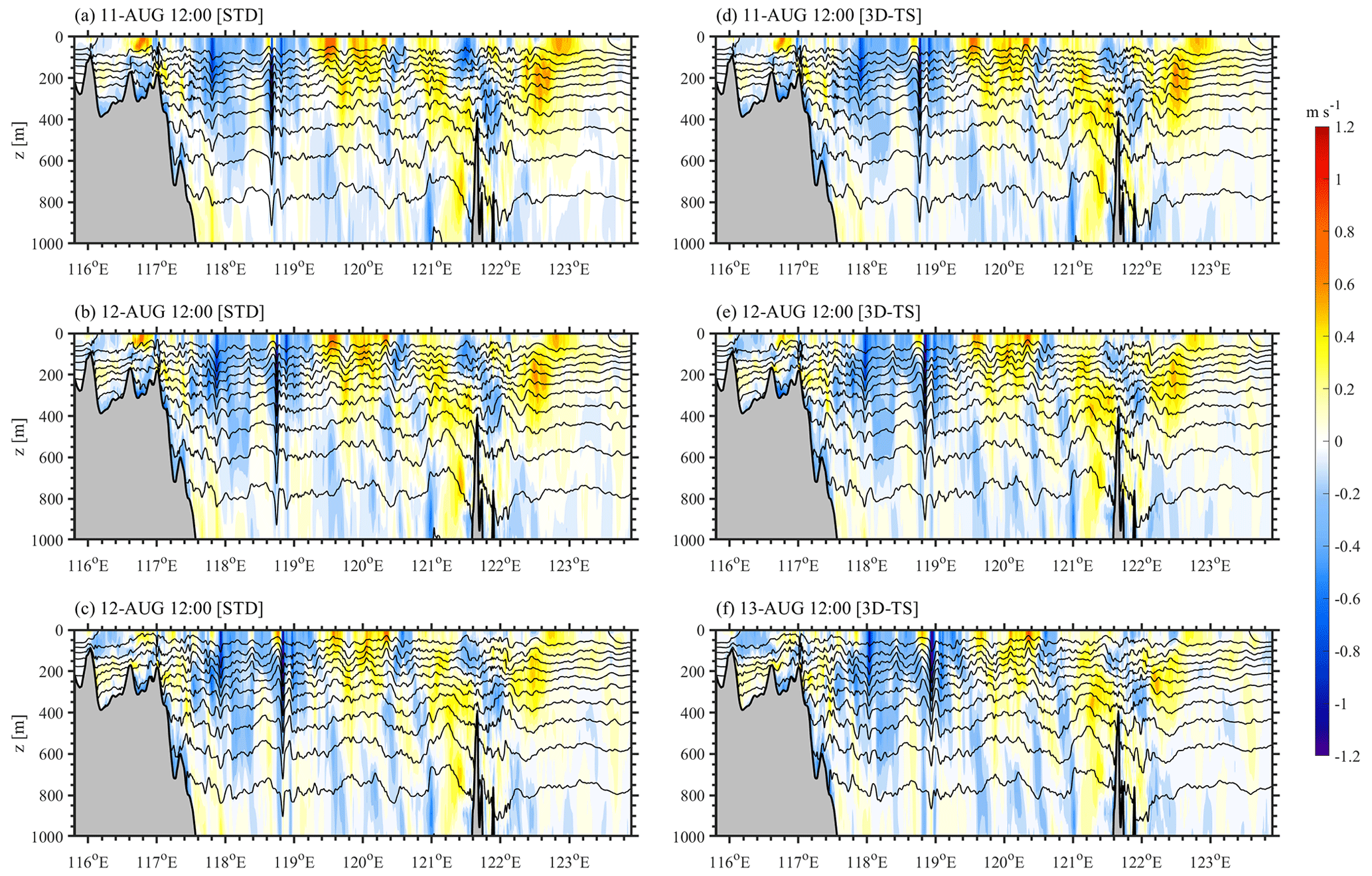
Figure C2 (a)–(c) Temperature isotherms (contours) and baroclinic velocities (shades) along the transect (dashed line in Fig. C1a) at 12:00 UTC on 11, 12 and 13 August in the standard experiment (Exp. 500m_8HARs), respectively. (d)–(f) Same as (a)–(c) but in the sensitivity experiment with horizontally inhomogeneous temperature and salinity (Exp. 3D-TS).