Adapting a deep convolutional RNN model with imbalanced regression loss for improved spatio-temporal forecasting of extreme wind speed events in the short to medium range

The number of wind farms and amount of wind power production in Europe, both on- and offshore, have increased rapidly in the past years. To ensure grid stability and on-time (re)scheduling of maintenance tasks and to mitigate fees in energy trading, accurate predictions of wind speed and wind power are needed. Particularly, accurate predictions of extreme wind speed events are of high importance to wind farm operators as timely knowledge of these can both prevent damages and offer economic preparedness. This work explores the possibility of adapting a deep convolutional recurrent neural network (RNN)-based regression model to the spatio-temporal prediction of extreme wind speed events in the short to medium range (12 h lead time in 1 h intervals) through the manipulation of the loss function. To this end, a multi-layered convolutional long short-term memory (ConvLSTM) network is adapted with a variety of imbalanced regression loss functions that have been proposed in the literature: inversely weighted, linearly weighted and squared error-relevance area (SERA) loss. Forecast performance is investigated for various intensity thresholds of extreme events, and a comparison is made with the commonly used mean squared error (MSE) and mean absolute error (MAE) loss. The results indicate the inverse weighting method to most effectively shift the forecast distribution towards the extreme tail, thereby increasing the number of forecasted events in the extreme ranges, considerably boosting the hit rate and reducing the root-mean-squared error (RMSE) in those ranges. The results also show, however, that such improvements are invariably accompanied by a pay-off in terms of increased overcasting and false alarm ratio, which increase both with lead time and intensity threshold. The inverse weighting method most effectively balances this trade-off, with the weighted MAE loss scoring slightly better than the weighted MSE loss. It is concluded that the inversely weighted loss provides an effective way to adapt deep learning to the task of imbalanced spatio-temporal regression and its application to the forecasting of extreme wind speed events in the short to medium range.

1 Introduction

Global warming demands ever more urgently that electricity generation is shifted away from fossil fuels and towards renewable energy sources. Although global demands for fossil fuels are not yet showing signs of decreasing, renewables are on the rise. In 2021, more than half of the growth in global electricity supply was provided by renewables, while the share of renewables in global electricity generation reached close to 30 %, having steadily risen over the past decades (IEA, 2021). Possessing the largest market share among the renewables, wind energy has managed to establish itself as a mature, reliable and efficient technology for electricity production and is expected to maintain rapid growth in the coming years (Fyrippis et al., 2010; Huang et al., 2015). Thanks to continued advancements in on- and offshore wind energy technology and the associated continued reduction in costs, wind power capacity could grow from having met 1.8 % of global electricity demand in 2009 to meeting roughly 20 % of demand in 2030 (Darwish and Al-Dabbagh, 2020). Indeed, many countries have already demonstrated that hybrid electric systems with large contributions of wind energy can operate reliably. For example, in as early as 2010, Denmark, Portugal, Spain and Ireland managed to supply between 10 % and 20 % of annual electricity demand with wind energy (Wiser et al., 2011), and the numbers have only risen since.

One of the main challenges to the deployment of wind energy, however, is its inherent variability and lower level of predictability than are common for other types of power plants (Lei et al., 2009; Chen and Yu, 2014; Li et al., 2018). Hybrid electric systems that incorporate a substantial amount of wind power therefore require some degree of flexibility from other generators in the system in order to maintain the right supply–demand balance and thus ensure grid stability (Wiser et al., 2011). Failing to manage this variability leads to scheduling errors which impact grid reliability and market-based ancillary service costs (Kavasseri and Seetharaman, 2009) while potentially causing energy transportation issues in the distribution network (Salcedo-Sanz et al., 2009) and increased risks of power cuts (Li et al., 2018). This is where wind speed forecasting can play a significant role. Incorporating high-quality wind speed forecasts, and, in return, wind power forecasts, into electric system operations gives the system more time to prepare for large fluctuations and can thereby help mitigate the aforementioned issues (Wiser et al., 2011). The variability in the short range, particularly over the timescale of 1–6 h, is found to pose the most significant operational challenges (Wiser et al., 2011; Li et al., 2018). The development of accurate wind speed forecasts in the short range has thus become increasingly important.

Short-term wind speed prediction is not just a key element in the successful management of hybrid electric power systems; it is also vital in the planning for necessary shutdowns in the face of extreme weather (Chen and Yu, 2014). Most existing turbines stop producing energy when either instantaneous gust speeds or averaged wind speeds exceed a threshold of around 25 m s⁻¹, after which the rotation of the blades is brought to a halt, and the turbine is essentially turned off (Burton et al., 2001). Using simulations of offshore wind power in Denmark, Cutululis et al. (2012) found that loss of wind power production during critical weather conditions can reach up to 70 % of installed capacity within an hour. Accurate forecasts of extreme wind events can therefore provide vital foresight to help prepare the electrical grid for such shutdowns as well as the duration of their downtime (Petrović and Bottasso, 2014).

There has been a particularly strong trend within the area of weather forecasting research towards data-driven, deep artificial neural networks (ANNs) (Jung and Broadwater, 2014). Such statistical forecasting models, however, are faced with a considerable challenge when tasked with the prediction of extreme events. Typically referring to the upper or lower tails of the data distribution, extreme events are inherently underrepresented during data-driven model learning and thus typically suffer from poor predictability and low forecasting bias in comparison to the bulk of the distribution. Improving the predictability of extreme events for data-driven models comprises an active area of research, and various approaches have been put forward, depending on the nature of the task. Class imbalances within classification tasks, for example, can be mitigated with a wide range of resampling strategies, either resampling the classes themselves (e.g. Batista et al., 2004) or the underlying probability density function (e.g. Mohamad and Sapsis, 2018; Hassanaly et al., 2021). The task may, furthermore, be treated as one-class classification (e.g. Deng et al., 2018; Goyal et al., 2020) or outlier exposure (e.g. Hendrycks et al., 2019).

While resampling strategies have also been proposed for imbalanced regression tasks (see, for example, Oliveira et al., 2021, for an application in the spatio-temporal setting), the machine learning literature on imbalanced regression tends to treat the problem as either anomaly detection (see, for example, Schmidl et al., 2022) or as a change of the loss function utilised during model learning. In the latter context, Ding et al. (2019) propose a novel loss function based on extreme value theory, called the extreme value loss (EVL), which is demonstrated to improve predictions of extreme events in time-series forecasting. The authors furthermore propose a memory-network-based neural network architecture to memorise past extreme events for better prediction in the future. Ribeiro and Moniz (2020) addressed the problem of imbalanced regression by proposing the squared error-relevance area (SERA) loss function, based on the notion of “relevance functions”. Yang et al. (2021), on the other hand, proposed the idea of distribution smoothing to address underrepresented or even missing labels in the label distribution and reduce unexpected similarities within the feature distribution that arise due to the label imbalance. The smoothed label distribution can then be used easily for re-weighting methods, where the loss function can be weighted by multiplying it by the inverse of the smoothed label distribution for each target. Such re-weighting of the loss function is a cost-sensitive remedy to data imbalance and has been used in the context of spatio-temporal weather forecasting by Shi et al. (2017).

Furthermore, a lot of work has been done in recent years on probabilistic weather forecasting, and many post-processing methods have been proposed to improve probabilistic forecasts. Post-processing is typically applied to ensemble weather forecasts or, for example, energy forecasts and attempts to correct biases exhibited by the system and improve overall performance (see, for example, Vannitsem et al., 2020, or Phipps et al., 2022) but has been explored to a lesser degree in the context of extreme event prediction. One approach to post-process ensemble forecasts for extreme events is to utilise extreme value theory, a review of which can be found in Friederichs et al. (2018). The authors propose separate post-processing toward the tail distribution and formulating a post-processing approach for the spatial prediction of wind gusts. Other authors have explored the potential of machine learning in this context. Ji et al. (2022), for example, investigate two deep-learning-based post-processing approaches for ensemble precipitation forecasts and compare these against the censored and shifted gamma-distribution-based ensemble model output statistics (CSG EMOS) method. The authors report significant improvements of the DL-based approaches over the CSG EMOS and the raw ensemble, particularly for extreme precipitation events. Ashkboos et al. (2022) introduce a 10-ensemble dataset of several atmospheric variables for machine-learning-based post-processing purposes and compare a set of baselines in their ability to correct forecasts, including extreme events. Alessandrini et al. (2019), on the other hand, demonstrate improved predictions on the right tail of the forecast distribution of analogue ensemble (AnEn) wind speed forecasts using a novel bias-correction method based on linear regression analysis, while Williams et al. (2014) show that flexible bias-correction schemes can be incorporated into standard post-processing methods, yielding considerable improvements in skill when forecasting extreme events.

As data-driven forecasting model, this paper investigates an adaptation of a deep convolutional long short-term memory (ConvLSTM) regression model, as proposed by Shi et al. (2015). The capability of deep ANNs to automatically and effectively learn hierarchical feature representations from raw input data has made such models particularly attractive to the area of spatio-temporal sequence forecasting, where complex spatial and temporal correlations are typically present in the data (Shi and Yeung, 2018; Amato et al., 2020; Wang et al., 2020). The ConvLSTM is an example of a ConvRNN model, which forms a synthesis of a convolutional neural network (CNN) and a recurrent neural network (RNN). CNNs are a class of feed-forward artificial neural networks, used primarily for data mining tasks involving spatial data, and have gained a lot of attention in the area of computer vision and natural language processing (Ghosh et al., 2020), while RNNs are known for their powerful ability to model temporal dependencies (Shi et al., 2015). By utilising the strengths of the CNN to capture spatial correlations and the RNN to capture temporal correlations in the data, ConvRNN models have demonstrated very promising forecasting ability in the spatio-temporal setting (Wang et al., 2020), outperforming both non-recurrent convolutional models and non-convolutional RNN models (Shi et al., 2015, 2017). As a multi-layered ConvRNN model, the deep ConvLSTM thus has the potential to effectively model the complex dynamics of the spatio-temporal wind speed forecasting problem.

In this paper an adaptation of a deep ConvLSTM regression model is applied to the task of the spatio-temporal prediction of extreme wind speed. The model is adapted with different types of imbalanced regression loss, and their efficacy in improving predictions on the right tail of the target wind speed distribution is compared. As such, this paper attempts to shed light on how the loss function of a deep learning model may be best adapted to improve forecasting performance on the distributional tail. Such improvement has practical relevance to wind energy applications where obtaining accurate predictions of extreme events are more desirable than accurate predictions of non-extremes, for example, in early-warning systems for wind farm operators. It is important to note, however, that while distributional tails in this work do not necessarily denote severe events in the absolute sense, the methodology of this work can be translated directly to cases where distributional tails denote actual hazardous events. The adapted models are, furthermore, compared against two base-line models, trained with mean absolute error (MAE) and mean squared error (MSE) loss. Forecast quality of all models is determined from a combination of categorical and continuous scores over a variety of intensity thresholds.

2 Methodology

2.1 Data collection and preprocessing

The wind speed data used in this work were downloaded from the Copernicus Climate Change Service Climate Data Store (CDS) of the ECMWF (see Hersbach et al., 2018), where different vertical levels are available. In this study, the focus lies on the 1000 hPa pressure level data which typically vary between 100 and 130 m above ground level, corresponding to the most common hub heights in the eastern part of Austria (main wind energy region). The U and V components of the horizontal wind velocity (in m s⁻¹) were thus taken at 1000 hPa from the “ERA5 hourly data on pressure levels from 1979 to present” dataset to calculate the scalar wind speed (computed as $\sqrt{U^{\mathrm{2}}+V^{\mathrm{2}}}$). The data were collected with a temporal resolution of 1 h between 1 January 1979 and 1 January 2021 (42 years) on a spatial grid over central Europe. Of these data, the last 2 years between 2019–2021 were held out as a test set. The 8 years between 2011–2019 were used for training and validation in the first part of the experiment, where the optimal model architecture for each of the investigated loss functions was determined using 4-fold cross-validation (with 6 years' training and 2 years' validation data). In the second part of the experiment, the optimal model architectures were then trained and validated on the entire 40 years of data between 1979–2019, using the 8 years between 2011–2019 as validation.

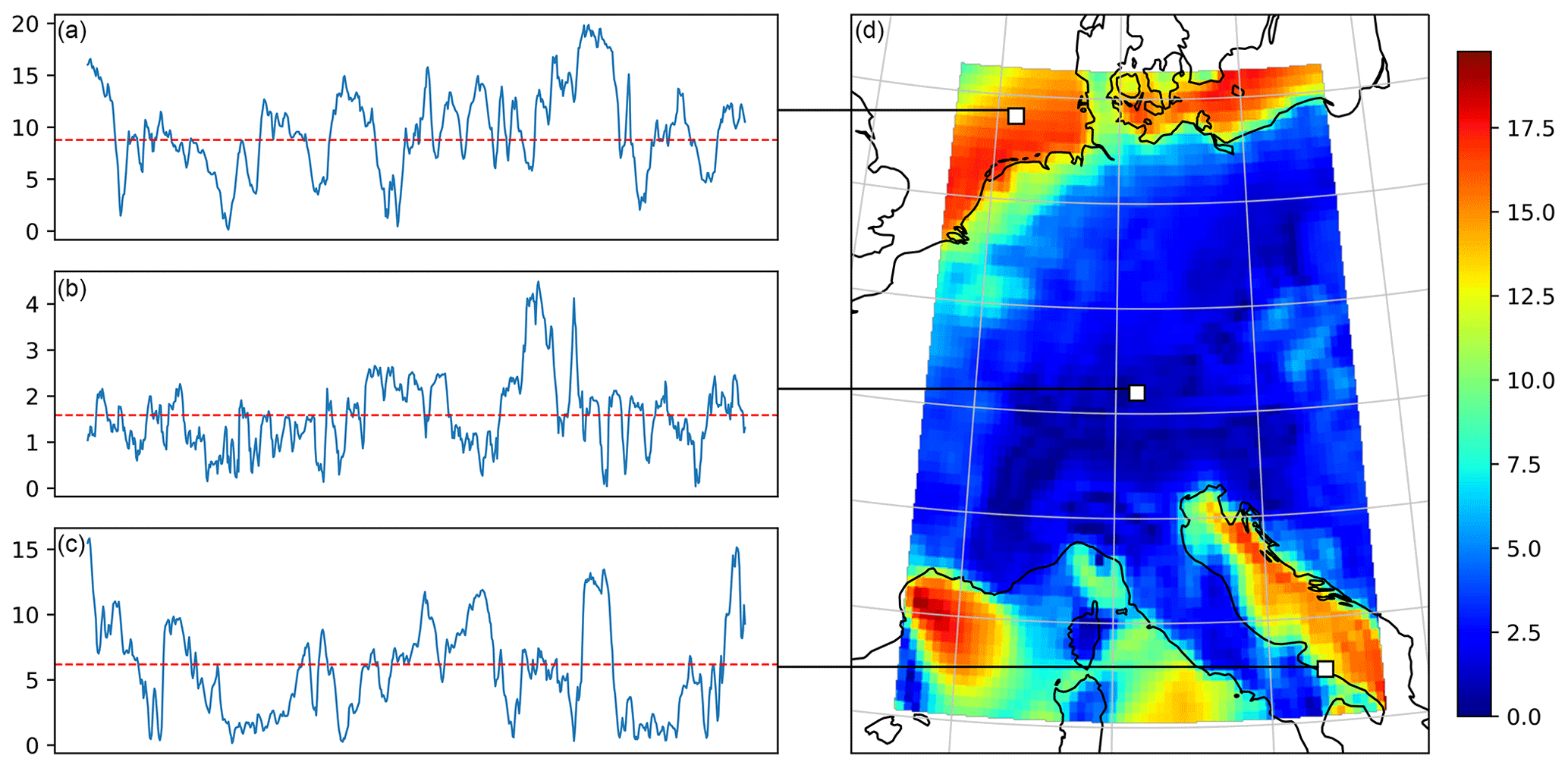
Figure 1 A visualisation of the wind speed data (in m s⁻¹). Panel (d) shows a colour map of an example data frame, overlaid on a cartographic map (central Europe) showing the coastlines of the region. On the left (a–c), the wind speed time series of three arbitrary locations (white squares) within the frame are plotted for the duration of 1 month, as well as the climatological means at these locations (dotted red lines).

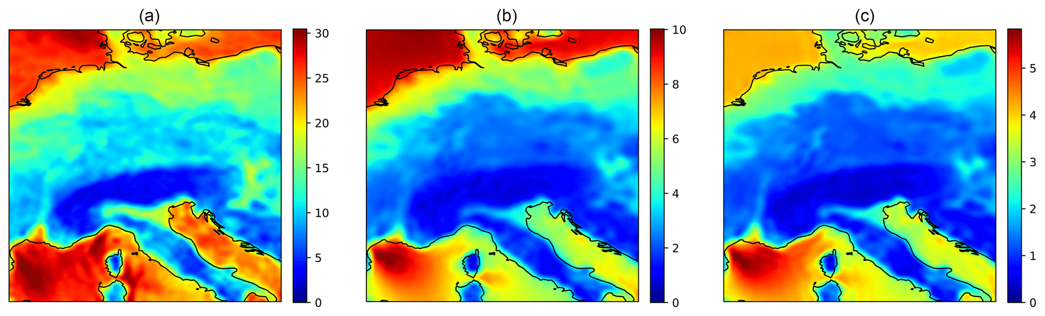
Figure 2 Colour maps of the maximum (a), mean (b) and standard deviation (c) of the wind speeds (in m s⁻¹) over the region. The figures display a sharp division of the statistics along the coastlines.

The spatial grid comprises 64 × 64 grid points between 40–56^∘ N and 3–19^∘ E, the spatial resolution being 0.25^∘ (≈ 28 km). This region was selected for its pronounced geographical variation, spanning land and sea regions, flat and mountainous areas, and different climatic regions. Interplay between these features can result in highly complex wind dynamics, which is why the application of deep learning was expected to be particularly promising. Moreover, the fine spatial resolution of 0.25^∘ was expected to be critical to capturing the complex fine-scale dynamics of a variable like low-level wind. The resolution also marks an important step forward for data-driven models to be truly competitive with state-of-the-art numerical weather prediction models, which are run at ≈ 0.1^∘ resolution (Pathak et al., 2022).

A visualisation of the data is provided in Fig. 1. The figure shows on the right an example spatial frame and on the left wind speed time series of three arbitrary locations over the duration of 1 month, including the climatological means at these locations. Evidently, the local climatological means (and by extension, the local wind speed distributions) vary substantially throughout the region, where striking differences in magnitude can be observed between the offshore and onshore regions. To highlight these spatial differences, Fig. 2 shows the maximum, mean and standard deviation of the wind speed over the region, which indeed unveil a sharp division of the statistics with the underlying coastlines of the region. In fact, extreme winds (e.g. larger than 25 m s⁻¹) seem to occur almost exclusively offshore: if there were stronger winds present over this region of mainland Europe between 1979 and 2021, then they have not been captured by the hourly ERA5 reanalysis.

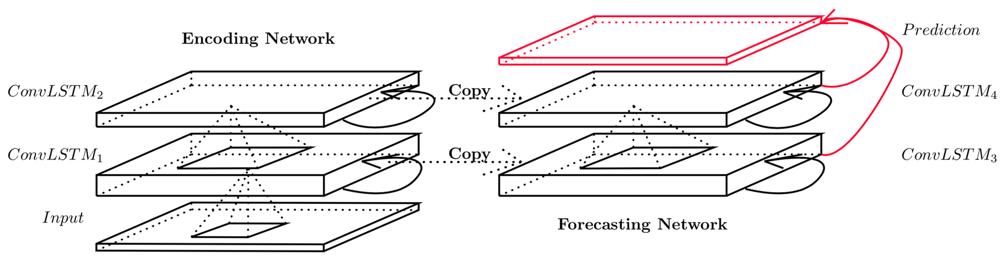
Figure 3 The multi-layered encoding–forecasting ConvLSTM network. The hidden states and cell outputs of the encoding network are copied to the forecasting network, from which the final prediction is made. © Shi et al. (2015). Used with permission.

Thus, rather than defining extreme winds in terms of their absolute severity, extreme winds are here defined in terms of their relative rarity at each coordinate. This definition focuses the forecasting problem on the right tails of the respective distributions at each coordinate, which ensures that the forecasting of extremes is conducted over the entire region, rather than only locally over some particularly dominant area (Fig. 2). By selecting a distributional percentile such as the 99th percentile, extreme winds are then defined as those wind speeds surpassing the percentile threshold of the wind speed sample distribution at the respective coordinate, i.e. wind speeds that are, indeed, rare at that coordinate (although not necessarily severe or hazardous in a absolute sense). For the remainder of this paper, the term “pth percentile threshold” refers always to the pth percentile of the target wind speed distribution at each coordinate. The above approach allows us to investigate forecasting improvements of extreme events more generally by looking at improvements on the tails of the respective distributions, regardless of the absolute values of the tails. Any improvements on the tails that result from the loss function modifications investigated in this paper can be swiftly translated to other data where the tails of the distributions do exclusively denote hazardous events.

The data were preprocessed at each coordinate using a Yeo–Johnson power transform (Yeo and Johnson, 2000) to make the local wind speed distributions more Gaussian-like and were subsequently standardised locally using zero-mean, unit-variance normalisation. The optimal parameter for stabilising variance and minimising skewness in the power transform was estimated through maximum likelihood, using scikit-learn (Pedregosa et al., 2011).

2.2 Model description

The model implemented for the task of spatio-temporal forecasting of wind speed is an adaptation of the convolutional long short-term memory (ConvLSTM) network, as proposed by Shi et al. (2015) for precipitation nowcasting. However, while Shi et al. (2015) trained their ConvLSTM model using cross-entropy loss, the model proposed here adjusts the ConvLSTM to the forecasting of extreme events by utilising two types of loss functions from the literature on imbalanced regression: weighted loss and the squared error-relevance area (SERA) loss.

As is common for spatio-temporal sequence forecasting, the deep ConvLSTM model architecture is adopted with an encoding–forecasting network structure, where both encoding and forecasting networks consist of several stacked ConvLSTM layers. As depicted in Fig. 3, the encoding ConvLSTM network compresses the input into a hidden state tensor, and the forecasting ConvLSTM network unfolds this hidden state into the final prediction (see Shi et al., 2015, for a mathematical description). The model is implemented as a multi-frame forecasting model, with 12 h input and 12 h prediction. This means that the model takes in tensors of size 12 × 64 × 64 as input, consisting of the previous 12 h of wind speed over the 64 × 64 grid, which are then encoded simultaneously through various hidden states of the encoding network and decoded through the decoding network into a subsequent 12 h prediction tensor of the same size (12 × 64 × 64).

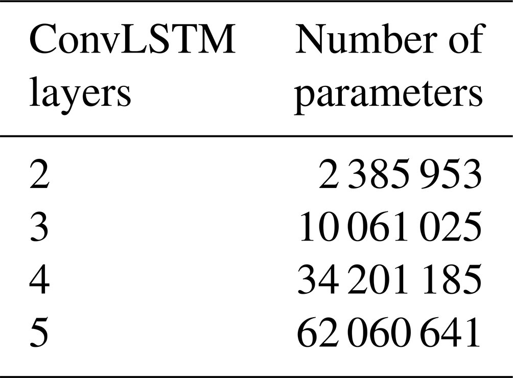
The model was implemented and trained using Pytorch (Paszke et al., 2019). In addition to the different loss functions, different model architectures with different numbers of ConvLSTM layers are investigated, ranging from two to five layers (in both the encoder and the forecasting networks). The numbers of parameters of all model architectures are shown in Table 1. In line with Shi et al. (2015), all layers utilise 3 × 3 kernels. The convolution over each successive filter operates such as to successively halve the spatial dimensions of the input, while the number of hidden states (features) is successively doubled (starting from 16 hidden states).

Table 1 The number of parameters of the ConvLSTM model with different numbers of layers.

The ConvLSTM is trained using mini-batch gradient descent with a batch size of 16 and used the adaptive moment estimation (Adam) as optimiser. Adam optimiser is a popular and reliable choice for deep learning neural networks which computes adaptive learning rates for each parameter of the model, based on their update frequency (see, for example, Ruder, 2017). As in Shi et al. (2017), the initial learning rate of the Adam optimiser is set to 10⁻⁴. During training, early stopping is performed on the validation set to ensure that the model with the lowest validation loss is saved as the best model and thus to avoid overfitting the model. The early-stopping mechanism is set up to stop training when the validation loss fails to decrease for 20 consecutive epochs.

These implementation and parameter choices were selected a priori based on the work of Shi et al. (2015) and Shi et al. (2017). Model performance may certainly be improved by performing a thorough hyper-parameter optimisation, but that is not the focus of this paper. The focus is set, instead, on providing a comparison of some of the different loss functions proposed in the literature for spatio-temporal imbalanced regression using deep learning in terms of their ability to improve the prediction of extreme wind speed. As such, the ConvLSTM model is adapted with two types of loss functions that have been proposed for imbalanced regression problems: weighted loss and squared error-relevance area (SERA) loss.

2.2.1 Weighted loss

Weighted loss consists of assigning a weight w(y) to each value in the input frame according to its target wind speed y. For a loss function L of the target y and prediction $\widehat{y}$ (consisting of N time frames of M × M spatial coordinates) and a weighting function w(y), the weighted loss L_W is computed as in Eq. (1). As weighted loss functions, both the weighted mean squared error (W-MSE) loss and the weighted mean absolute error (W-MAE) loss are investigated.

$$\begin{array}{}\text{(1)}& L_{\mathrm{W}}(\widehat{y},y)={\displaystyle \frac{\mathrm{1}}{N}}\sum _{n=\mathrm{1}}^N\sum _{i,j=\mathrm{1}}^{M}w\left(y_{n,i,j}\right)\cdot L({\widehat{y}}_{n,i,j},y_{n,i,j})\end{array}$$

As weighting function both an inverse weighting function and a simple linear weighting function are investigated. The inverse weighting function computes the weights in proportion to the inverse of the data distribution for each target, as suggested by Yang et al. (2021). For a continuous target distribution, this typically implies discretising the distribution into intervals (see, for example, Shi et al., 2017), where all predictions within an interval are weighted by the same weight. Due to the definition of extreme events in this paper in terms of local percentile thresholds, the target distribution is discretised into intervals spanning the percentage of the distribution between percentile p and 100. For a set of increasing percentiles 𝒫={p_k}, all targets $p_k\le y<p_{k+\mathrm{1}}$ are then weighted proportionally to the inverse of the percentage between p_k and 100, i.e. $w\left(y\right)\propto \mathrm{1}/(\mathrm{100}-p_k)$. We utilise a range of integer percentiles $\mathcal{P}=\mathit{\left\{}{p}_k\right|k\in [\mathrm{50},\mathrm{99}]\mathit{\}}$ and normalise weights such that the interval between percentiles 50 and 51 is given unit weight. As such, weights increase inversely from 1 up until a weight of 50 (given to target values $p_{\mathrm{99}}\le y\le p_{\mathrm{100}}$). All values smaller than the 50th percentile (p₅₀) are also given unit weight. This results in the weighting function shown in Eq. (2), which is also presented graphically in Fig. 4.

$$\begin{array}{}\text{(2)}& \begin{array}{rl}& w_{\text{inv}}\left(y\right)=\\ & \left\{\begin{array}{ll}\mathrm{1}& \text{if }y<p_{\mathrm{50}}\\ \mathrm{50}\cdot \frac{\mathrm{1}}{\mathrm{100}-k}& \text{if }{p}_k\le y<p_{k+\mathrm{1}}\text{ for }k\in [\mathrm{50},\mathrm{99}]\end{array}\right.\end{array}\end{array}$$

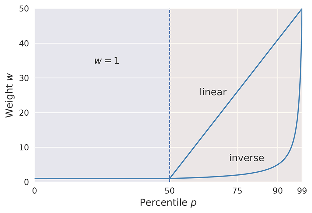
Figure 4 Weighting functions used to construct either the inversely weighted mean squared error (W-MSE_inv) and mean absolute error (W-MAE_inv) or the linearly weighted mean squared error (W-MSE_lin) and mean absolute error (W-MAE_lin).

The linear weighting function is constructed analogously as shown in Eq. (3): target values y<p₅₀ are similarly given unit weight, while weights for target values $p_k\le y\le p_{k+\mathrm{1}}$ are increased linearly from 1 to 50 for percentiles $k\in [\mathrm{50},\mathrm{99}]$. The function is also presented graphically in Fig. 4.

$$\begin{array}{}\text{(3)}& \begin{array}{rl}& w_{\text{lin}}\left(y\right)=\\ & \left\{\begin{array}{ll}\mathrm{1}& \text{if }<p_{\mathrm{50}}\\ k-\mathrm{49}& \text{if }{p}_k\le y<p_{k+\mathrm{1}}\text{ for }k\in [\mathrm{50},\mathrm{99}]\end{array}\right.\end{array}\end{array}$$

2.2.2 Squared error-relevance area loss

As another approach to combating data imbalance, the squared error-relevance area (SERA) loss, as proposed by Ribeiro and Moniz (2020), is investigated. The SERA loss is based on the concept of a relevance function $\mathit{\varphi }:\mathcal{Y}⟶[\mathrm{0},\mathrm{1}]$, which maps the target variable domain 𝒴 onto a [0,1] scale of relevance. The relevance function ϕ is determined through a cubic Hermite polynomial interpolation of a set of “control points”. The set of control points $S=\mathit{\{}\langle y_k,\mathit{\varphi }(y_k),{\mathit{\varphi }}^{\prime }(y_k)\rangle {\mathit{\}}}_{k=\mathrm{1}}^s$ are user-defined points where the relevance may be specified, which are typically local minima or maxima of relevance and thus all have derivative ${\mathit{\varphi }}^{\prime }\left(y_k\right)=\mathrm{0}$ (Ribeiro and Moniz, 2020).

In this implementation, the method is implemented on a per-coordinate basis, and the local 99th percentile (p₉₉) at each coordinate is fixed as the point of maximum relevance. The point of minimum relevance is varied between the 90th percentile (p₉₀), the 75th percentile (p₇₅) and the 50th percentile (p₅₀) in order to investigate how this choice affects forecasting performance. The interpolation in all cases is carried out according to Ribeiro and Moniz (2020) using the piecewise cubic Hermite interpolating polynomial (pchip) algorithm. The relevance function obtained for two control points (e.g. p₉₀ and p₉₉) is shown in Fig. 5.

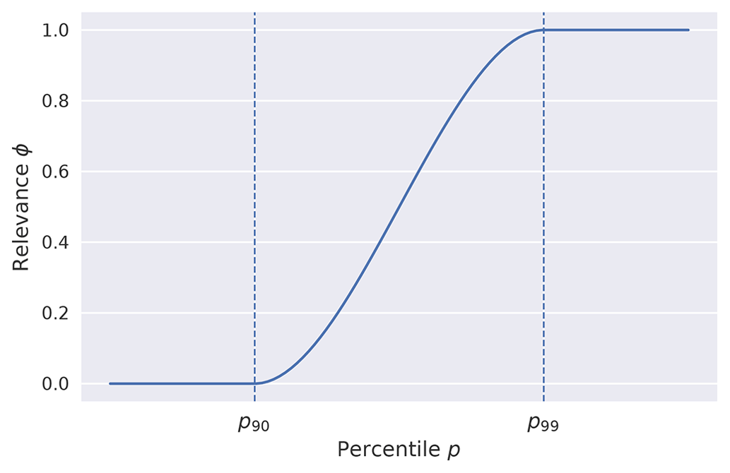
Figure 5 The relevance function ϕ obtained by interpolating the control point of minimum relevance and the control point of maximum relevance, chosen as the 90th percentile (p₉₀) and the 99th percentile (p₉₉) in this figure, using the pchip interpolation algorithm.

Defining D^t as the subset of data pairs for which the relevance of the target value is greater than or equal to a cut-off t, i.e. $D^t=\mathit{\{}\langle x_i,y_i\rangle \in D|\mathit{\varphi }\left(y_i\right)\ge t\mathit{\}}$, the squared error-relevance SER_t of the model with respect to the cut-off t is then computed as follows:

$$\begin{array}{}\text{(4)}& {\text{SER}}_t=\sum _{i\in D^t}({\widehat{y}}_i-y_i{)}^{\mathrm{2}},\end{array}$$

where ${\widehat{y}}_i$ and y_i are the ith prediction and target values, respectively. The curve obtained by plotting SER_t against t is decreasing and monotonic (Ribeiro and Moniz, 2020) and provides an overview of how the magnitudes of the prediction errors change on subsets comprising varying degrees of relevant samples (t=0 representing all samples and t=1 representing only the most relevant samples). Finally, the squared error-relevance area (SERA) is defined as the area under the SER_t curve:

$$\begin{array}{}\text{(5)}& \text{SERA}=\underset{\mathrm{0}}{\overset{\mathrm{1}}{\int }}{\text{SER}}_t\mathrm{d}t.\end{array}$$

The smaller the area under the curve is, the better the model is. It can be noted that assigning uniform relevance values to all data points recovers the MSE loss. We also note that, regardless of the choice of relevance function, the SERA loss utilises the complete set of given samples in its computation, not solely a subset, as the integral in Eq. (5) starts at t=0, and SER_t=0 denotes all samples with relevance values greater than or equal to 0, i.e. all samples.

2.3 Forecast evaluation

In order to evaluate the predictions of the ConvLSTM against observations, the model's hit rate ($H=\frac{a}{a+c}$), false alarm ratio (FAR $=\frac{b}{a+b}$), threat score ($\text{TS}=\frac{a}{a+b+c}$) and frequency bias ($B=\frac{a+b}{a+c}$) are analysed, where a denotes the number of hits, b the number of false alarms, c the number of missed hits and d the number of correct negatives obtained by the model. The hit rate, false alarm ratio and threat score are routinely used by the UK Met Office to evaluate warnings (Hogan and Mason, 2012) and have also been used by Shi et al. (2015) to evaluate the ConvLSTM model for precipitation nowcasting, while the frequency bias provides valuable information on whether the model tends to overcasting or undercasting.

These scores are computed for a set of intensity thresholds corresponding to the local 50th, 75th, 90th, 95th, 99th and 99.9th percentiles of the observed sample distributions at each coordinate, which are computed using the training set. In order to obtain an aggregated result over all forecasts made by a model, the elements in the contingency table (a, b, c and d) are aggregated over all forecasts, and the scores are computed subsequently from the aggregated contingency table.

Since the above categorical scores work on the basis of a forecast being correct as long as it surpasses the same threshold t as the observed event, they are able to give an indication of the frequency of errors, while they are unable to give an indication of the magnitude of the errors between the forecast and observations. In order to include a comparison of error magnitudes in the analysis, the root-mean-squared error (RMSE) between (continuous-valued) predictions and observations is utilised. Unlike the categorical scores, the RMSE is computed here between two consecutive percentile thresholds: for a particular forecast and observation, and thresholds p₁ and p₂, the RMSE is computed between all pairs of forecast and observation values (f,o) where the observation values lie between p₁ and p₂, i.e. $p_{\mathrm{1}}\le o<p_{\mathrm{2}}$. The total RMSE for those thresholds is then computed as an aggregate over all forecasts and observations of the model. This approach serves to give an indication of the typical magnitude of errors of the forecasts of a model over a particular percentile range of the observations.

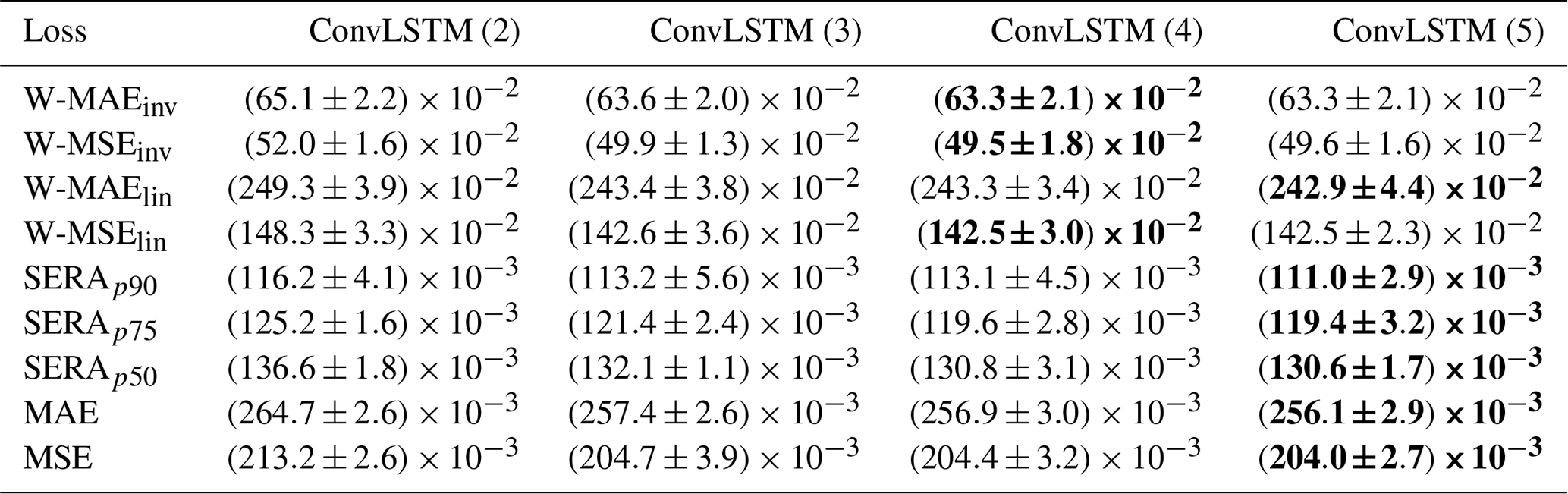
Table 2 Minimum validation loss as obtained by the ConvLSTM network with the number of layers ranging from two to five (denoted in brackets) and trained with each different loss function. Values are presented as the mean ± 1 standard deviation from the 4-fold cross-validation. The lowest minimum validation loss reached, and thus the optimal network architecture, is emphasised in boldface for each loss function. Where multiple architectures obtained the same minimum validation loss, the simpler architecture is given precedence.

In the next section the results obtained from combining the multi-layered ConvLSTM network with the various loss functions are presented. The optimal number of layers for each model is determined from the minimum validation loss obtained by the networks as averaged over the 4-fold cross-validation process (conducted over the 8 years of data between 2011–2019). The optimal models are then re-trained using the entire 40 years of data between 1979–2019 (using the 8 years between 2011–2019 as validation), and their results are compared on the held-out test set comprising the 2 years between 2019–2021.

3 Results

3.1 Validation loss

Table 2 shows the minimum validation loss obtained by the ConvLSTM network with the number of layers ranging between two and five, as trained with either inversely weighted loss (W-MAE_inv and W-MSE_inv), linearly weighted loss (W-MAE_lin and W-MSE_lin), SERA loss or standard MAE or MSE loss. The SERA loss is denoted with a subscript denoting the first control point used, with the second control point fixed at the local 99th percentile (p₉₉) for each coordinate. Results are shown as the mean ± 1 standard deviation from the 4-fold cross-validation. The minimum validation loss for each loss function has been emphasised in boldface, indicating the optimal number of network layers for each loss function. In cases where the mean validation loss is equal for multiple numbers of layers, the smallest number of layers, and thus the simplest model, was given precedence.

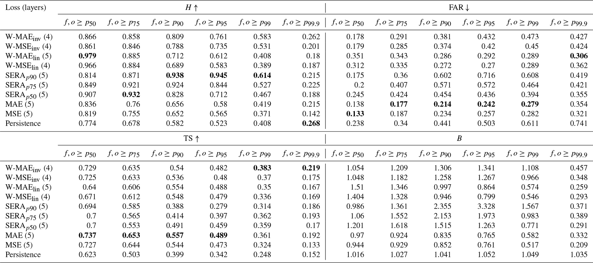
Table 3 Comparison of hit score (H), false alarm ratio (FAR), threat score (TS) and frequency bias (B) of the ConvLSTM network trained with each different loss function. Scores are presented for wind forecasts f and observations o exceeding local intensity thresholds varying between the 50th (p₅₀) and 99.9th (p_99.9) percentiles, aggregated over lead time. The optimal number of network layers used for each loss function is given in brackets after the name of the loss function. The persistence forecast is included in the table for reference. For each intensity threshold, the best scores are emphasised in boldface (where applicable).

3.2 Comparison over intensity thresholds

The models were then re-trained using the entire 40 years of data between 1979–2019 (using the 8 years between 2011–2019 as validation) with the corresponding optimal number of network layers (henceforth indicated in brackets after the name of the respective loss function with which the network was trained). The following comparison shows the models' performance on the held-out test set (years 2019–2021). Table 3 shows a comparison of the hit score (H), false alarm ratio (FAR), threat score (TS) and frequency bias (B) for wind forecasts f and observations o exceeding local intensity thresholds between the 50th (p₅₀) and the 99.9th (p_99.9) percentiles, aggregated over all lead times. The persistence forecast, which simply consists of a repetition of the final input frame, is included in the table for reference.

The table shows that the imbalanced regression losses generally result in significant increases in the hit rate as compared with the standard MAE or MSE loss, indicating that more of the true occurrences of the events were captured by the model. Any improvement in the hit rate is, however, accompanied by an increase in the false alarm ratio. This suggests that in order to capture more of the events, the models are invariably producing more false alarms. This behaviour is particularly pronounced where there is substantial overcasting, i.e. a frequency bias substantially greater than 1. This can be best noticed for the SERA_p90 model at the intensity threshold p₉₅, where a massive frequency bias of 332.8 % results in the model successfully capturing a spectacular 94.5 % of true events (the hit rate) at the cost of 71.6 % of forecasted events being false alarms (the false alarm ratio).

The threat scores can give an overall idea of forecasting performance and, as such, suggest that the SERA-trained models investigated here can only be considered superior to the MSE-trained model for the p₉₉ threshold (except for SERA_p90, which scores worse) and for the p_99.9 threshold. Compared to the MAE loss, the SERA-trained models typically score worse threat scores for all thresholds, except for the SERA_p75 model which manages to be on par at intensity thresholds p₉₉ and p_99.9. As a matter of fact, none of the models trained with imbalanced regression loss achieve threat scores superior to the MAE trained model for thresholds p₅₀–p₉₅, although the inversely weighted losses generally achieve comparable scores, and the linearly weighted losses achieve comparable scores for p₉₀ and p₉₅. Between the linearly weighted losses, the W-MAE_lin achieves better scores for higher thresholds (p₉₀ onward). The W-MAE_lin also achieves slightly better scores than either inversely weighted losses for thresholds p₉₀ and p₉₅. The inversely weighted losses dominate, however, for the extremely high thresholds p₉₉ and p_99.9, outperforming all other loss functions on these thresholds. Performance for all models on threshold p_99.9 must be interpreted with caution, however, since threat scores on this threshold approach those obtained from the persistence forecast. Indeed, in terms of hit rate, none of the models investigated in this paper are able to successfully predict events of the 99.9th percentile threshold better than persistence. Similarly, for the 99th percentile, the standard MAE and MSE and the linearly weighted MAE and MSE result in hit rates comparable to persistence, highlighting the inability of these standard loss functions to capture extremely rare events.

As compared with the standard MAE loss, the W-MAE_inv manages to boost the hit rate significantly across all intensity thresholds, while some degree of overcasting and increased false alarms will have to be allowed for. For p₉₀, for example, the usage of the W-MAE_inv achieves an increase in H from 0.656 (standard MAE) to 0.809, with the FAR rising from 0.214 to 0.381. Even for p₉₉, a significant increase in H is achieved, from 0.419 (standard MAE) to 0.583, with the FAR rising more drastically, however, from 0.279 to 0.473. Overcasting and FAR values can be reduced substantially, however, using the linear weighting method. For p₉₀ events, the W-MAE_lin increases the FAR more conservatively from 0.214 (standard MAE) to 0.286 while still boosting H from 0.656 to 0.712. The table shows that a small boost in H can still be expected for p₉₅ events, but beyond that, the linearly weighted MAE or MSE offers no improvements (with hit rates dropping to values comparable with persistence). Depending then on what magnitude of false alarms that is acceptable, and for what percentile of extreme events the loss function is desired to offer improvement, either the linear or the inverse weighting methods can be utilised. Between all usages of the MAE and MSE, either weighted or unweighted, the MAE returns higher hit rates and higher threat scores at the cost of an increased false alarm ratio and an increased frequency bias.

Compared to the weighted loss functions, the SERA offers something of an extreme case, allowing hit rates to be boosted spectacularly but at a considerable loss of forecasting performance (as judged by reduced threat scores, increased overcasting and increased false alarms). The primary control point of the SERA loss does offer a way to mitigate this behaviour, however. For example, reducing this control point from p₉₀ to p₇₅ and then to p₅₀ (while keeping the second control point fixed at p₉₉) shows a striking reduction in frequency bias, false alarms and hit rates for intensity thresholds between p₉₀–p₉₉, while threat scores, and thus overall forecasting performance, generally improve.

Table 4 As Table 3 but presented for the root-mean-squared error (RMSE), which is computed between all pairs of forecast and observation values (f,o) where the observation values lie between p₁ and p₂, i.e. $p_{\mathrm{1}}\le o<p_{\mathrm{2}}$.

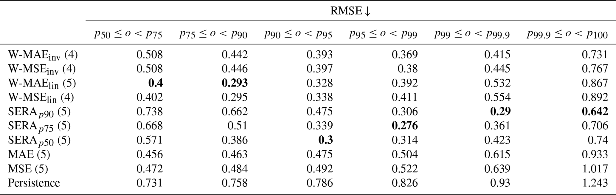
Table 4 shows the root-mean-squared error (RMSE) obtained from the continuous forecasts and observations of the different models. Unlike Table 3, the RMSE is computed between all pairs of forecast and observation values (f,o) where the observation values lie between p₁ and p₂, i.e. $p_{\mathrm{1}}\le o<p_{\mathrm{2}}$. Again, the persistence forecast is included for reference. The table shows that the imbalanced regression losses tend to result in lower RMSE scores, as compared to the standard MAE and MSE loss, for increasingly rare observation values. It is interesting to note that while the SERA-trained models generally appear to result in heavy overcasting and highly inflated false alarm rates (Table 3), the RMSE scores suggest that increasing the first control point of the SERA loss results in shifting the domain of minimal RMSE towards the higher percentiles. Between the inverse and linear weighting methods, the RMSE scores echo the interpretations from Table 3, with the linear method appearing more adept (lower RMSE) around the central percentiles and the inverse method more adapt towards the higher percentiles.

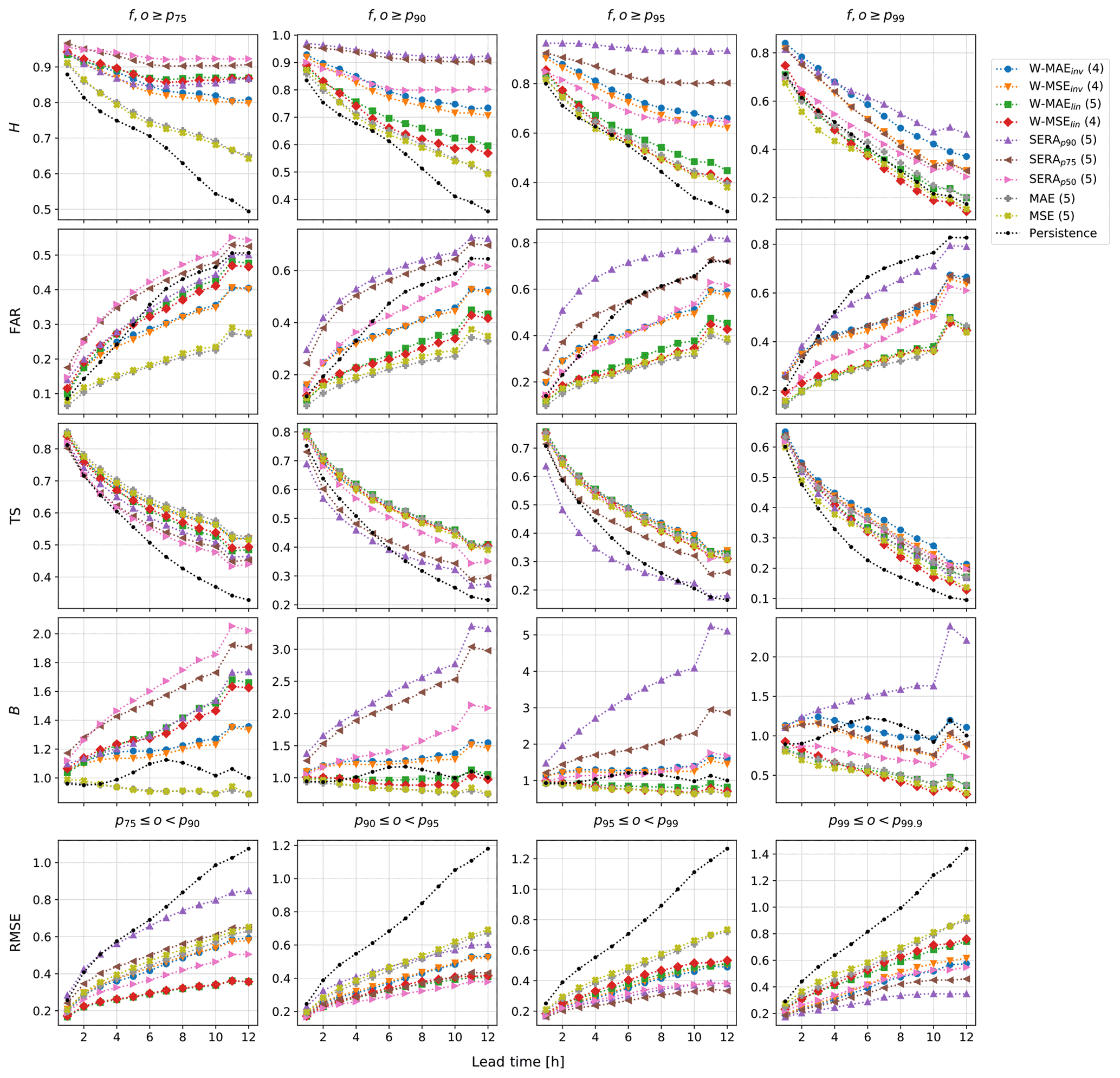
Figure 6 Comparison of the hit score (H), false alarm ratio (FAR), threat score (TS), frequency bias (B) and root-mean-squared error (RMSE) of the ConvLSTM network trained with each different loss function, plotted over lead time (in hours) and various percentile intensity thresholds. The optimal number of network layers used for each loss function is given in brackets after the name of the loss function. The label “persistence” refers to the persistence forecast.

3.3 Temporal assessment

The performance of the models is investigated further in Fig. 6, where the scores obtained by each model are plotted over lead time (in hours) for the 75th (p₇₅), 90th (p₉₀), 95th (p₉₅) and 99th (p₉₉) percentile intensity thresholds in particular. Once again the persistence forecast is included for reference. Not only does the figure provide a temporal picture of forecasting performance, but the different models can also readily be compared to the “baseline” persistence forecast (dotted black line). The figure clearly shows that the imbalanced regression losses result in sustained hit rates H over lead time, while false alarm rates FAR and frequency bias B suffer large increases, as compared with the standard MAE and MSE. Indeed, none of the imbalanced regression loss functions succeed in increasing either H or TS without inflating FAR or B to some degree; in fact, typically the stark improvements in H result in degraded TS scores (most clearly visible for the SERA models on thresholds p₇₅, p₉₀ and p₉₅).

Although the inverse weighting, the linear weighting and the SERA loss each provide a different way to balance forecasting performance towards improved hit rates, they achieve this aim with varying success. For example, not only are the heavily inflated B and FAR scores produced by the SERA models not typically qualities of reliable forecasting systems, the models also do not succeed in keeping TS scores on par with the standard MAE and MSE loss; spectacular improvements in H thus seem to be primarily a result of extreme overcasting bias, not actually improved predictive power. Compared with the SERA loss, the inversely weighted losses, W-MAE_inv and W-MSE_inv, sustain H scores over lead time to a lesser degree but nevertheless show strong improvements over the standard MAE and MSE while showing no apparent loss in TS over lead time (in fact, showing substantial improvement for threshold p₉₉) and inflating FAR and B scores much more conservatively. Although the linear weighted losses display more conservative FAR and B scores still, it is evident that any improvements in H cease rather quickly beyond a threshold of p₉₅.

Lastly, the RMSE scores show clearly how forecasts gradually lose precision with increasing lead time. It is interesting to note that the relationship appears to be roughly linear. The imbalanced regression losses consistently show improved RMSE scores over lead time as compared with the standard MAE, MSE and persistence, with lowest scores on the higher percentiles between p₉₅–p_99.9 achieved by the SERA losses, followed by the inversely weighted losses and lastly the linearly weighted losses.

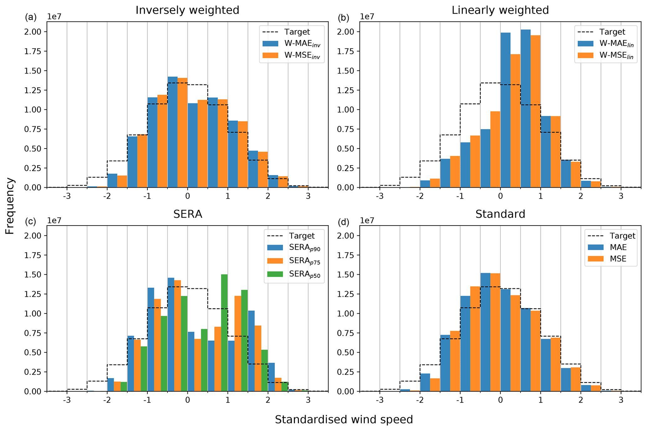
Figure 7 Histograms of forecast distributions of the ConvLSTM trained with the various different loss functions investigated in this paper, compared to the underlying distribution of the observations in the test set, which are labelled as “Target” (dotted black line). (a) The inversely weighted losses. (b) The linearly weighted losses. (c) The SERA loss with different primary control points (with the secondary control point fixed at p₉₉). (d) The standard MAE and MSE losses. The distributions were sampled with a step size of 0.5 (standardised wind speed).

3.4 Forecast distributions

Figure 7 provides a set of histograms showing the forecast distributions of the ConvLSTM trained with the various different loss functions. The figure is split up into the inversely weighted losses (top left), the linearly weighted losses (top right), the SERA loss with different primary control points (bottom left) and the standard MAE and MSE losses (bottom right). Included in the histograms is the underlying distribution of the observations in the test set, labelled as “Target” (dotted black line). The distributions were sampled with a step size of 0.5 (standardised wind speed).

The figure clearly shows how the different types of loss functions result in the forecast distribution being shifted towards the right tail in rather distinct fashions. Comparison of the different forecast distributions with the target distribution highlights the different undercasting and overcasting behaviour as observed from the frequency bias (B) in Table 3. While all imbalanced regression loss functions appear to shift more predictions towards the right tail of the target distribution, they evidently conserve the shape of the target distribution to varying degrees, with the SERA loss and the linear weighting resulting in rather large distortions and heavy overcasting on the right tail. In fact, the SERA loss shifts predictions towards the right tail of the target distribution with such severity that this results in an additional peak on the right side of the forecast distribution; the peak evidently shifted further towards the right tail as the primary control point varies from p₅₀ to p₉₀. Inverse weighting clearly samples the target distribution with better success and limits overcasting to a better degree than either linear weighting or SERA loss.

3.5 Permutation tests

In this section, some more insight is given into the predictions made by the ConvLSTM network by discussing feature importance. In order to determine the importance of each of the 12 input frames that are used by the ConvLSTM to make its predictions, a permutation test was carried out on the input data. For each input frame at time T (−11–0), all input frames from the test set were randomly shuffled (full fields) at time T, essentially nullifying the information flow from this input frame. Then the model predictions from these permuted inputs were obtained, and a skill score S (in %) was computed between the RMSE of the original prediction and target (RMSE_org) and the permuted prediction and target (RMSE_perm), i.e. $S=(\mathrm{1}-{\mathrm{RMSE}}_{\mathrm{org}}/{\mathrm{RMSE}}_{\mathrm{perm}})\times \mathrm{100}$. A score of 0 % indicates no change in RMSE, a score of 100 % indicates maximum increase in RMSE and negative scores indicate decrease in RMSE due to the permuted inputs. Not only does this offer insight into the importance that each input frame carries in the ultimate prediction, but it also helps to ensure that the model is, in fact, basing its predictions on the information flow between consecutive input frames rather than simply resorting to forecasting climatology.

Figure 8 Results from the permutation tests. The figure shows the RMSE skill score (in %) between the targets and the normal predictions of each of the models and the targets and the predictions resulting from randomly permuting the inputs at time frame T. A score of 0 % indicates no change in RMSE, a score of 100 % indicates maximum increase in RMSE and negative scores indicate decrease in RMSE due to the permuted inputs. (b) The linearly weighted losses. (c) The SERA loss with different primary control points (with the secondary control point fixed at p₉₉). (d) The standard MAE and MSE losses.

Figure 8 presents the RMSE skill scores as aggregated over the test set, obtained by the different models. The figure shows that scores for all models get particularly large as the permuted input frame T approaches 0 h. This shows clearly that the last input frame at time T=0 hours bears most importance to the predictions, which is to be expected from a regression model predicting the continuation of a sequence from time frame T=0 onward. The standard MAE and MSE loss show a fairly steady rise in RMSE skill score from time $T=-\mathrm{11}$ towards T=0, showing that more “recent” frames of the input tend to bear more importance in the predictions (with the exception of a slight drop (for the MAE loss) or stagnation (for the MSE loss) at $T=-\mathrm{2}$ and $T=-\mathrm{1}$). The imbalanced regression losses, however, show an additional jump in RMSE skill scores peaking around ca. $T=-\mathrm{8}$ and $T=-\mathrm{7}$, after which scores fall considerably before gradually climbing again to peak at T=0. Earlier input frames bearing more importance on the predictions may suggest that the models trained with the various imbalanced regression losses utilise more of the long-term information flow in the inputs to improve the forecasting on the extremes.

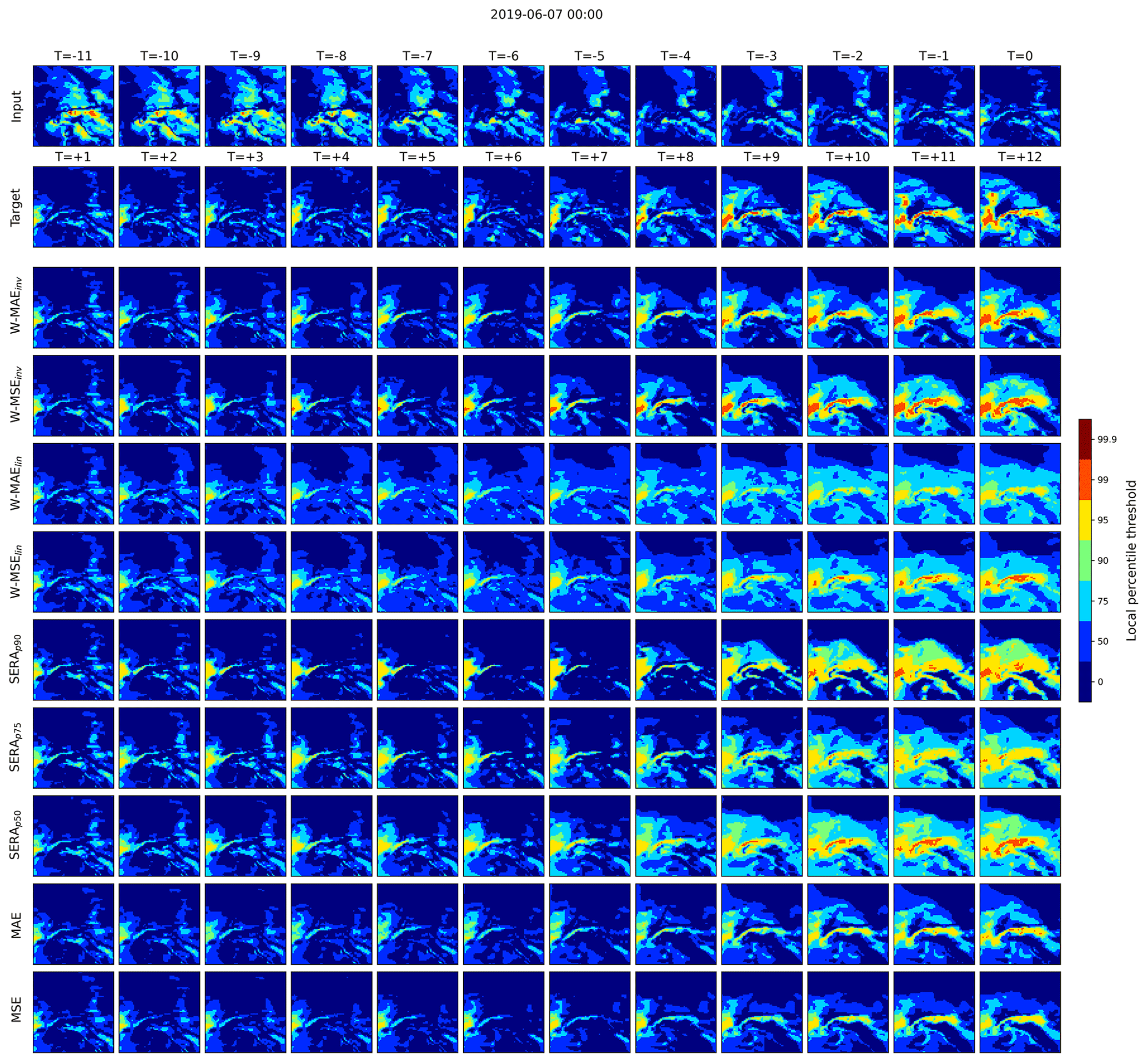
Figure 9 An example forecast from the ConvLSTM network trained with the various different loss functions. The first row from the top displays the 12 input frames, the second row the succeeding 12 target frames and the following rows the 12 predicted frames of the models. T refers to the index of the frame (in hours), with T=0 denoting the last input frame and $T=+\mathrm{12}$ denoting the final target and prediction frames. Rather than showing the raw predictions, the predictions are categorised into binary events using percentile intensity thresholds.

Figure 10 As Fig. 9.

Figure 11 As Fig. 9.

3.6 Forecast examples

Finally, Figs. 9, 10 and 11 present visualisations of three selected example forecasts made by the ConvLSTM model trained with the different loss functions investigated in this paper, highlighting their respective strengths and weaknesses. In each figure, the first row from the top displays the 12 winput frames, the second row displays the succeeding 12 target frames and the following rows display the 12 predicted frames of the various models. T refers to the index of the frame (in hours), with T=0 denoting the last input frame and $T=+\mathrm{12}$ denoting the final target and prediction frames. Rather than showing the raw predictions, the predictions are categorised into categorical events using the local percentile intensity thresholds. In this fashion, the figures show precisely where the different types of events are predicted and where not.

All three examples show a target observation of an intensification of extreme winds, each resulting in a patch of 99th percentile events between from ca. $T=+\mathrm{8}$ onward. In each case, the standard MAE and MSE loss either forecast the intensification to some degree but largely fail to capture the 99th percentile events (Figs. 9 and 11), or they fail to forecast the event completely (Fig. 10). In comparison, the inversely weighted losses (W-MAE_inv and W-MSE_inv) show a much improved ability to forecast the right intensification and the right degree of extreme events, with the W-MAE_inv performing clearly better in Fig. 11 than the W-MSE_inv. From the forecasts of the linear weighted losses, the heavy frequency bias on lower percentile events (as discussed previously) can be easily distinguished, although some 95th and 99th percentile events are captured. Between the SERA_p90, SERA_p75 and SERA_p50 models, the examples clearly reflect the heavily inflated frequency bias towards the higher percentile events, with bias increasing more towards the 99th percentile as the primary control point varies from p₅₀ to p₉₀ (in line with the behaviour discussed in Fig. 7).

4 Discussion

The results presented in this paper indicate that the multi-layered convolutional long short-term memory (ConvLSTM) network can be adapted to the task of spatio-temporal forecasting of extreme wind events through the manipulation of the loss function. By analysing the forecasts of the ConvLSTM trained with the various imbalanced regression loss functions investigated in this work, utilising various different scores and intensity thresholds, as well as comparing forecast distributions and visualised forecast examples, it is clear that inverse weighting, linear weighting and squared error-relevance area (SERA) loss each provide viable ways of shifting predictive performance of the ConvLSTM towards the tail of the target distribution. Furthermore, from the permutation tests, it is clear that all ConvLSTM models utilise the information flow from the inputs to compute the forecasts, and it may be that networks trained with the imbalanced regression losses may utilise more information flow from long-term dynamics than the baseline models trained with MAE and MSE loss.

The results indicate that hit rates and RMSE scores can be greatly improved for extreme events up until the 99th percentile threshold, after which hit rates drop considerably and cease to surpass persistence scores. Table 3 and Fig. 6 demonstrate clearly, however, that improvements in hit rate are accompanied by proportionate increases in frequency bias and false alarm ratios. When this trade-off is particularly extreme, as in the case of the SERA loss with the control points investigated here, not only do threat scores begin to suffer considerably, but also the model loses its viability as a reliable forecasting model, with false alarm ratios massively inflated. Lowering the primary control point, however, from the 90th percentile (p₉₀) to the 50th percentile (p₅₀) limits this behaviour for extreme events between the 90–99th percentiles (see Fig. 6).

The linear weighting method, instead, shows minimal improvement in hit rate over the standard MAE and MSE on intensity thresholds above p₉₀, as it increases forecasting bias mostly closer to the median and not the tails (Fig. 7), which means that it does not appear to put enough relative weight on the extreme tails. It should be noted, however, that the linear weighing method tested here was tested only with one slope, and other slopes may yield better results. Shi et al. (2017), for example, utilised a linear weighting method for precipitation nowcasting using a trajectory gated recurrent unit (TrajGRU) network and reported improved performance at higher rain-rate thresholds as compared with the standard MSE and MAE (based on the threat score and the Heidke skill score).

Between the three types of imbalanced regression loss investigated in this work, the inverse weighting method appears to strike the best balance between improved hit rate versus increased frequency bias and false alarm ratio. Not only does the inverse weighting method sample the target distribution more accurately (Fig. 7), but frequency bias and false alarm rates are also substantially less inflated than the SERA loss over all percentile thresholds between p₇₅–p₉₉ (with the slight exception for the SERA_p50 model and high thresholds), while hit rates are substantially better than linear weighting for thresholds p₉₀–p_99.9, and threat scores are improved for thresholds p₉₉ and p_99.9. The W-MAE_inv appears to strike this balance slightly better than the W-MSE_inv.

This discussion will proceed by mentioning a number of possible extensions of this work. One disadvantage of utilising the entirety of available data is that many of the input-target samples containing extreme winds are samples where extreme winds are present in both the input as well as the target. Examples where there are no extremes present in the input, but the target is showing onsets of extremes, are disproportionately rare in the data, although they clearly represent a more interesting problem for early-warning systems. Improvements of a deep-learning-based early-warning system for the onsets of extreme winds could thus be obtained by focusing model learning on precisely such training samples, rather than employing all available samples.

This work may, furthermore, be extended by taking a multivariate approach to wind speed forecasting, whereby other atmospheric variables are included in the input of the model, which is an approach that is already being pursued in the community (see, for example, Racah et al., 2017; Marndi et al., 2020; Xie et al., 2021). Marndi et al. (2020) suggest the utilisation of temperature, humidity and pressure, as Cadenas et al. (2016) have found these to be significantly more important than other atmospheric variables to the task of wind forecasting. Xie et al. (2021) use these same three variables, as well as the 1 h minimum and maximum temperature, while Racah et al. (2017) use a much larger set of 16 atmospheric variables, albeit for the classification of large-scale extreme weather events and not for the regression of wind speed. It may also be worthwhile to consider other atmospheric variables such as the convective available potential energy (CAPE) and deep-layer wind shear (DLS) due to their strong correlation with severe convective storm activity such as the occurrence of thunderstorms and supercells (see, for example, Rädler et al., 2015; Tsonevsky et al., 2018; Chavas and Dawson II, 2021). Another possible extension would be to implement categorical scores directly in the loss function (see, for example, Lagerquist and Ebert-Uphoff, 2022) or even combine the ConvLSTM with a so-called physics-aware loss function (see, for example, Schweri et al., 2021; Cuomo et al., 2022).

Finally, it should be noted that while the ConvLSTM has proven itself to be highly effective at modelling complex spatio-temporal patterns, other models have since been proposed as promising improvements to the ConvLSTM for the task of spatio-temporal sequence forecasting. Most notably, the PredRNN and its successor PredRNN++, proposed by Wang et al. (2017) and Wang et al. (2018), respectively, have been demonstrated to be superior to the ConvLSTM for the task of video frame prediction by maintaining a global memory state rather than constraining memory states to each ConvLSTM module individually. Other alternative approaches include the usage of functional neural networks (FNNs) (see Rao et al., 2020) or generative adversarial networks (GANs) (see Gao et al., 2022). Such models may be of interest to the meteorological community pursuing data-driven, spatio-temporal forecasting.

5 Conclusions

In this paper, a deep learning approach to the task of spatio-temporal prediction of wind speed extremes was explored, and the role of the loss function was investigated. To this end, a multi-layered convolutional long short-term memory (ConvLSTM) network was adapted to the task of spatio-temporal imbalanced regression by training the model with a number of different imbalanced regression loss functions proposed in the literature: inversely weighted loss, linearly weighted loss and squared error-relevance area (SERA) loss. The models were trained and tested on reanalysis wind speed data from the European Centre for Medium-Range Weather Forecasts (ECMWF) at 1000 hPa, providing multi-frame forecasts of horizontal near-surface wind speed over Europe with a 12 h lead time and in 1 h intervals, using the preceding 12 h as input. By standardising the data based on the local wind speed distributions at each coordinate, the definition of an extreme event was focused on its relative rarity rather than its absolute severity, with extreme winds thus considered in terms of their local distributional percentile.

The model forecasts were analysed and compared with a variety of scores and over various intensity thresholds. After determining the optimal number of network layers for the ConvLSTM trained with the various different loss functions, an extensive comparison was made between the different loss functions and two baseline models trained with either mean absolute error (MAE) or mean squared error (MSE) loss. The results show that the imbalanced regression loss functions investigated in this paper can be used to substantially improve hit rates and RMSE scores over the baseline models, however, at the cost of increased frequency bias and false alarm ratios. The SERA loss provides an extreme case of this behaviour, typically at the additional cost of reductions in threat score, although results are heavily dependent on the loss function's so-called control points. The linear weighting method shows some ability to boost hit rates while keeping frequency bias and false alarm ratio comparatively low, although the utility of the method is lost for extreme events beyond the 90th percentile intensity threshold, with predictions heavily biased towards the median of the distributions rather than the right tail. Inverse weighting is concluded to strike the best trade-off between improved hit rates and sustained threat scores versus increased frequency bias and false alarm ratio, across various thresholds of extreme events up until the 99th percentile intensity threshold, with the weighted MAE loss scoring slightly better than the weighted MSE loss. The inverse weighting method, furthermore, results in a better sampling of the target distribution as compared with the linear weighting or the SERA loss. Out of the different imbalanced regression loss functions investigated in this work, the inverse weighting loss is thus concluded to be most effective at adapting the ConvLSTM to the task of imbalanced spatio-temporal regression and its application to the forecasting of extreme wind speed events in the short to medium range. With these results, this work is hoped to provide a valuable contribution to the area of deep learning for spatio-temporal imbalanced regression and its application to wind energy forecasting research.