the Creative Commons Attribution 4.0 License.
the Creative Commons Attribution 4.0 License.
 | 09 May 2023
ClinoformNet-1.0: stratigraphic forward modeling and deep learning for seismic clinoform delineation
Jinyu Zhang
Xiaoming Sun
Zhengfa Bi
Deep learning has been widely used for various kinds of data-mining tasks but not much for seismic stratigraphic interpretation due to the lack of labeled training datasets. We present a workflow to automatically generate numerous synthetic training datasets and take the seismic clinoform delineation as an example to demonstrate the effectiveness of using the synthetic datasets for training. In this workflow, we first perform stochastic stratigraphic forward modeling to generate numerous stratigraphic models of clinoform layers and corresponding porosity properties by randomly but properly choosing initial topographies, sea level curves, and thermal subsidence curves. We then convert the simulated stratigraphic models into impedance models by using the velocity–porosity relationship. We further simulate synthetic seismic data by convolving reflectivity models (converted from impedance models) with Ricker wavelets (with various peak frequencies) and adding real noise extracted from field seismic data. In this way, we automatically generate a total of 3000 diverse synthetic seismic datasets and the corresponding stratigraphic labels such as relative geologic time models and facies of clinoforms, which are all made publicly available. We use these synthetic datasets to train a modified encoder–decoder deep neural network for clinoform delineation in seismic data. Within the network, we apply a preconditioning process of structure-oriented smoothing to the feature maps of the decoder neural layers, which is helpful to avoid generating holes or outliers in the final output of clinoform delineation. Multiple 2D and 3D synthetic and field examples demonstrate that the network, trained with only synthetic datasets, works well to delineate clinoforms in seismic data with high accuracy and efficiency. Our workflow can be easily extended for other seismic stratigraphic interpretation tasks such as sequence boundary identification, synchronous horizon extraction, and shoreline trajectory identification.
- Article
(14849 KB) - Full-text XML
- BibTeX
- EndNote


Seismic stratigraphic interpretation is a crucial step for understanding the evolutionary history information of the sedimentary basin based on seismic data and is particularly applicable to the sedimentary basin where well data are lacking or unavailable (Nanda, 2021). With the development of seismic data from 2D to 3D and the dramatic increase in the amount of data, the automatic realization of seismic stratigraphic interpretation is the trend. Currently, deep learning has been successfully applied in geophysical interpretation tasks such as fault detection (Huang et al., 2017; Di et al., 2018; Zhao and Mukhopadhyay, 2018; Wu et al., 2019), horizon interpretation (Lowell and Paton, 2018; Wu and Zhang, 2018), and salt body delineation (Shi et al., 2019). However, deep-learning-based automatic seismic stratigraphic interpretation is not discussed much due to the lack of the corresponding training labels. In this work, we take the seismic clinoform delineation task as an example to discuss how to solve the problem of a lack of training datasets by stratigraphic forward modeling and further train a deep neural network for efficient and accurate seismic stratigraphic interpretation.
The clinoform and the clinothem are widely studied as important sedimentary archives and underpin sequence stratigraphy (Patruno and Helland-Hansen, 2018; Pellegrini et al., 2020). Rich (1951) first introduced the concepts of clinoform and clinothem and proposed the partitioning of deposited surfaces into undaform, clinoform, and fondoform. Steel and Olsen (2002) redefined clinoform as a deposition surface containing undaform and fondoform and divided the clinoform into topset, foreset, and bottomset. In this work, we use the term clinoform to describe a surface with a sigmoidal shape, inclined and dipping toward the basin over a wide range of spatial and temporal scales (Rich, 1951; Bates, 1953; Asquith, 1970; Pirmez et al., 1998; Adams and Schlager, 2000; Steel and Olsen, 2002; Patruno and Helland-Hansen, 2018; Ramon-Duenas et al., 2018), and the term clinothem to describe the clinoform-bounded sedimentary body that records the incremental filling of a sedimentary basin (Patruno and Helland-Hansen, 2018; Ramon-Duenas et al., 2018). In addition, in the field of oil and gas exploration, clinoforms have attracted the attention of oil and gas companies in recent years because most of them are low-permeability mudstones or cement, making them potential reservoir units for hydrocarbon resources (Cummings and Arnott, 2005; Sydow et al., 2013; Holgate et al., 2013, 2014; Patruno et al., 2018).
The geometry of the clinoform can provide information about paleodepth, shoreline changes, and the changes in sediment supply and accommodation (Pellegrini et al., 2020). Clinoform can be divided into three components according to geometry. The topset is characterized by low-gradient strata (typically<0.1∘) at the top and is dominated by muddy siltstone and fine to medium-grained sandstone. The foreset is characterized by the steepest slope in the middle and is dominated by muddy siltstone and fine sandstone. The bottomset is characterized by a low gradient toward the basin and is dominated by turbidite sandstone (Patruno and Helland-Hansen, 2018; Ramon-Duenas et al., 2018; Pellegrini et al., 2020).
Currently, the delineation of the three components of the clinoform (topset, foreset, and bottomset) in seismic data is still mainly based on human interpretation by experienced geologists and therefore remains a labor-intensive task, especially in 3D seismic volumes. With the recent development of artificial intelligence, deep learning methods have been successfully applied to automate data interpretation tasks in various fields. The convolutional neural network (CNN) method has been proven to be the most powerful method in semantic segmentation (Ronneberger et al., 2015; He et al., 2016; Badrinarayanan et al., 2017; Chen et al., 2018). Recently, the mainstream networks for semantic segmentation are U-net proposed by Ronneberger et al. (2015) and DeepLabV3+ proposed by Chen et al. (2018). However, it is challenging to apply the CNN method in solving geoscience problems including the seismic stratigraphic interpretation because of the lack of a large number of training datasets and the related labels (Karpatne et al., 2018; Bergen et al., 2019; Di et al., 2020).
To solve this problem, using synthetic labeled datasets for training a CNN model is considered an effective methodology (Araya-Polo et al., 2018; Wu et al., 2020; Guo et al., 2021; Puzyrev et al., 2022; Jessell et al., 2022). In this work, we consider performing numerical stratigraphic forward modeling (SFM) to generate numerous synthetic datasets with labels. SFM has been widely used in the study of sequence stratigraphy over the last decades (Martin et al., 2009; Burgess et al., 2012; Sylvester et al., 2015; Harris et al., 2016). Many mathematical and physical models have been proposed to simulate the evolution of sedimentary basins by using various numerical algorithms to obtain synthetic stratigraphic states in full consideration of thermal subsidence, uplift, changes in sediment supply, and various sediment transport and deposition processes (Warrlich et al., 2008; Shafie and Madon, 2008; Burgess et al., 2012; Hawie et al., 2015; Salles et al., 2018). While most of the previous work performs SFM to fit the stratigraphic model of a specific basin by carefully choosing a set of modeling parameters, we perform stochastic SFM to generate numerous models by randomly choosing various sets of parameters.
In this paper, we develop a workflow (Fig. 1) to automatically generate synthetic seismic data and corresponding labels and use the synthetic datasets to train a CNN for seismic clinoform delineation. We first use a numerical SFM method, modified from pyBadlands (Salles et al., 2018) to generate a synthetic porosity model (Fig. 1d) and relative geologic time model (Fig. 1e) of clinoform layers with inputs of a randomly but properly chosen initial topography surface (Fig. 1a), sea level changes (Fig. 1b), and thermal subsidence curve (Fig. 1c). Then we use an interpolation method and a velocity–porosity relationship proposed by Krief et al. (1990) to build an impedance model (Fig. 1f) and at the same time calculate a slope volume (Fig. 1g) from the corresponding depth model of clinoform layers. Finally, we perform depth-to-time conversion to the impedance model, convolve it with a Ricker wavelet with a random peak frequency (Fig. 1j), and add real noise to generate a synthetic seismic image (Fig. 1h). At the same time as generating the synthetic seismic data, we also automatically obtain the corresponding stratigraphic labels of relative geologic time and clinoform delineation (Fig. 1i). After generating various clinoform seismic data and corresponding labels, we use them to train a CNN modified from DeepLabv3+ for automatic clinoform delineation in seismic data. We demonstrate the performance of the trained network on both synthetic and field seismic data.
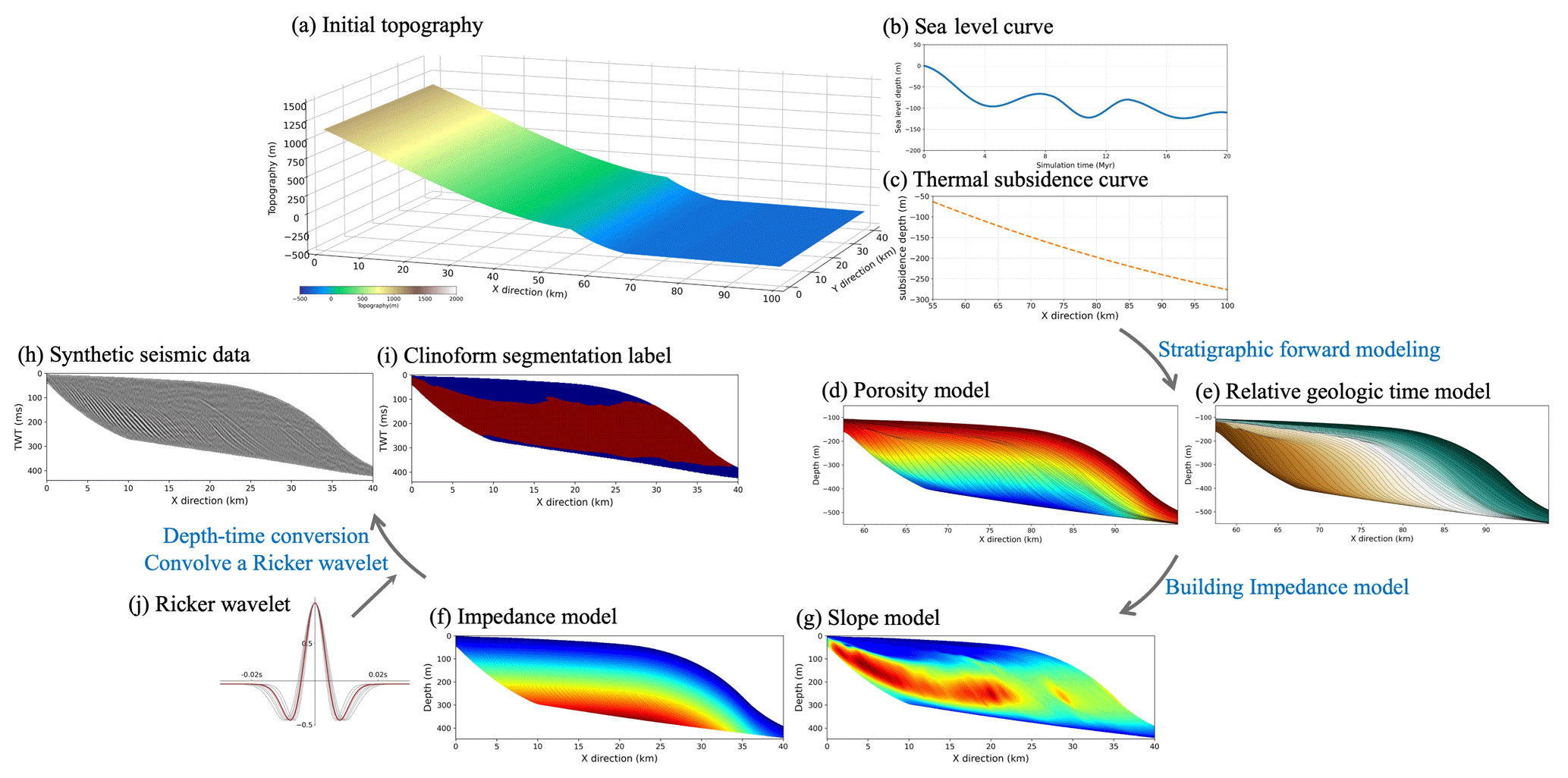
Figure 1Workflow of generating the synthetic clinoform seismic data and corresponding label. We first use a randomly generated (a) initial topography, (b) sea level curve, and (c) thermal subsidence curve to obtain (d) a porosity model and (e) relative geologic time by stratigraphic forward modeling. Then we use an interpolation method and velocity–porosity relationship to obtain the corresponding (f) P wave impedance model and (g) slope model. Finally, we obtain the (h) synthetic seismic data and (i) the corresponding segmentation label by depth–time conversion, convolving with (j) a Ricker wavelet with a random peak frequency and adding real noise.
In this section, we implement a workflow of geological and geophysical forward modeling processes (Fig. 2) to automatically generate diverse synthetic clinoform seismic data and corresponding labels to train a CNN for seismic stratigraphic interpretation. The black boxes in Fig. 2 contain the SFM process based on pyBadlands (Salles et al., 2018), and the blue boxes in Fig. 2 contain the geophysical forward modeling processes of generating synthetic seismic data and corresponding segmentation labels. In this workflow, we first randomly generate diverse SFM inputs, such as initial topography, sea level curve, rainfall patterns, uplift, and subsidence. We then simulate numerous stratigraphic models of clinoform layers using stratigraphic forward modeling with these diverse model inputs. After obtaining these stratigraphic models of clinoform layers, we perform an interpolation method and a velocity–porosity relationship to build the velocity and impedance models. We further use the velocity model generated in the previous step to convert the stratigraphic models from the depth domain to the time domain. Finally, we convolve the reflectivity model (converted from the impedance model) with a Ricker wavelet to generate the synthetic seismic data and add real noise to improve the realism of the synthetic seismic data.
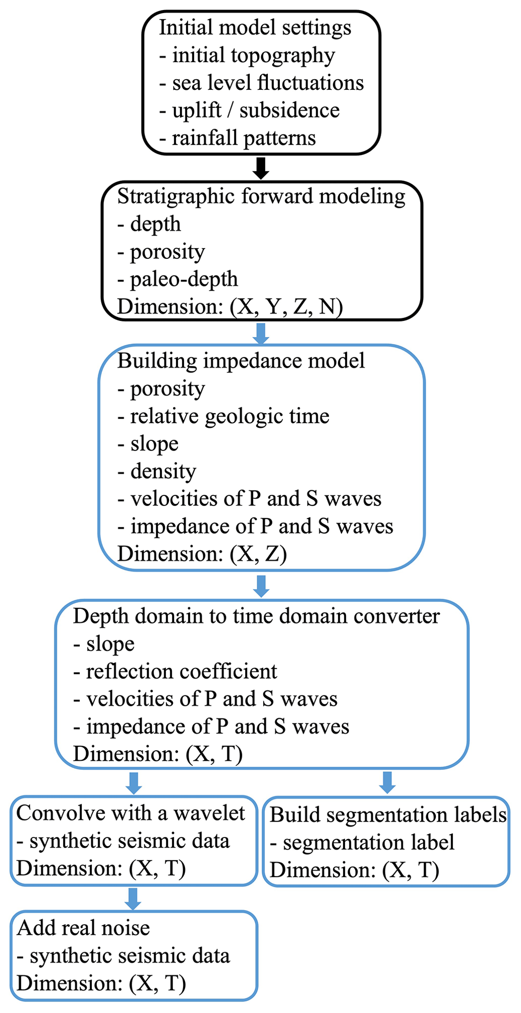
Figure 2Workflow of generating diverse synthetic clinoform seismic data and corresponding segmentation labels. The black boxes contain the steps of the stratigraphic simulation process in pyBadlands (Salles et al., 2018). X and Y represent the length of inline and crossline directions, respectively. N represents the number of clinoform layers generated in the simulation. The blue boxes contain the process of generating synthetic clinoform seismic data and corresponding segmentation labels. Z represents the vertical magnitude of the interpolated formation attributes in the depth domain, and T represents the vertical magnitude of the interpolated formation attributes in the time domain.
2.1 Stratigraphic forward modeling
Many SFM methods have been proposed to simulate the evolution of sedimentary basins by using various numerical algorithms to obtain synthetic clinoform layers in full consideration of thermal subsidence, uplift, changes in sediment supply, and various sediment transport and deposition processes (Warrlich et al., 2008; Shafie and Madon, 2008; Burgess et al., 2012; Hawie et al., 2015; Salles et al., 2018). In this study, we use the SFM method implemented in pyBadlands (Salles et al., 2018) to simulate numerous stratigraphic models of clinoform layers. PyBadlands is a long-term surface evolution model that simulates sediment transport and deposition from source to sink (Salles and Hardiman, 2016; Salles et al., 2018; Ding et al., 2019).
At each time step of the simulation, the sedimentary structure of the clinoform layers is mainly controlled by the rate of accommodation change (δA) and the rate of sediment-supply change (δS). The rate of accommodation change (δA) reflects the spatial capacity for accommodating sediments and is mainly related to thermal subsidence, sea level fluctuations, etc. The rate of sediment-supply change (δS) is mainly related to the erosion of source domain determined by rainfall patterns, topography, rock erodibility, etc. (Schlager, 1993; Muto and Steel, 1997; Hawie et al., 2015; Neal et al., 2016). When δS≥δA, clinothem typically accumulates and moves toward the sedimentary basin, and when δS≤δA, clinothem typically moves and retrogrades toward the continental shelf (Patruno and Helland-Hansen, 2018; Pellegrini et al., 2020).
The whole workflow of simulating numerous stratigraphic models of clinoform layers is summarized in the black boxes in Fig. 2. In this simulation process, we generate 200 clinoform layers for each model and set the grid size and time step as 100 m×100 m and 0.1 Myr, respectively. Moreover, in order to obtain diverse geometric clinoform layers, the initial topography, sea level curve, thermal subsidence, and rainfall patterns are randomly chosen from some predefined ranges in Table 1.
Table 1Summary of initial parameter ranges for stratigraphic forward modeling.
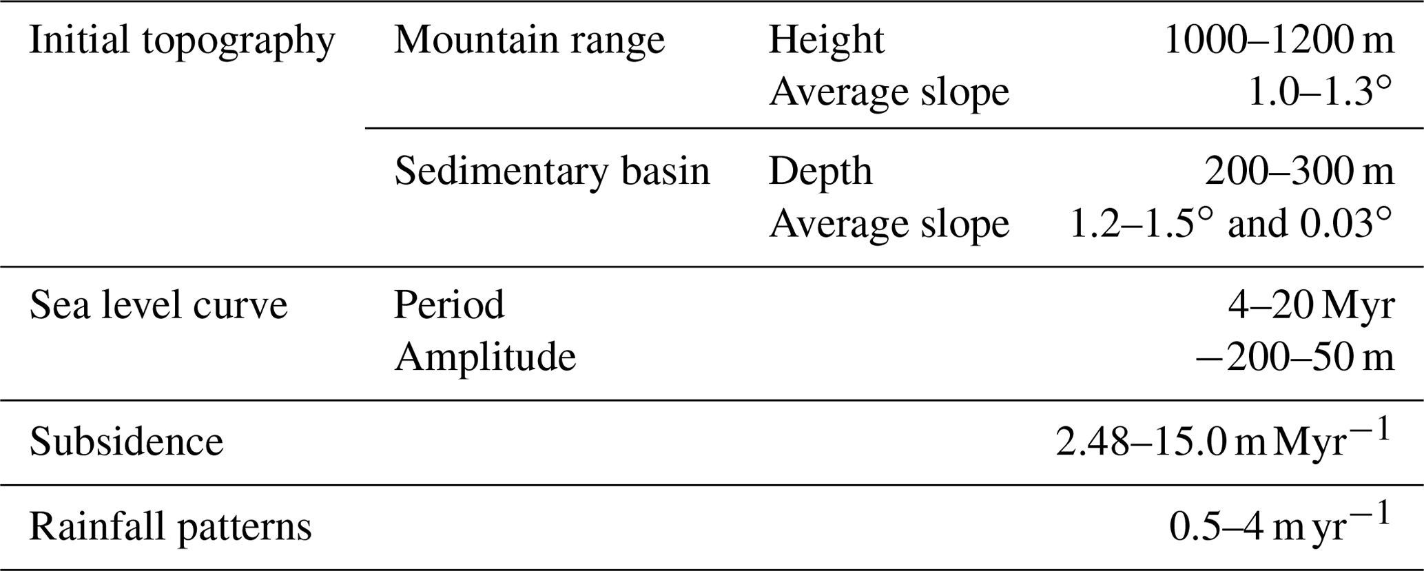
As shown in Fig. 3a, the initial topography for simulation has a spatial scale of 100 km (x direction) by 40 km (y direction) and a grid size of 100 m by 100 m. The mountain range (erosion region) is 55 km (x direction) by 40 km (y direction), while the sedimentary basin (sedimentary region) is 45 km (x direction) by 40 km (y direction). We randomly set the highest altitude of the mountain range within 1000–1200 m and set the average slope in the range between 1.0 and 1.3∘. The sedimentary basin is divided into two parts: an inclined basin margin region and a relatively flat basin center region. The average slope of the inclined basin margin area and the flat basin center area is set to 1.2–1.5∘ and 0.03∘, respectively. In this paper, we perform 3D stratigraphic forward modeling to build 3D stratigraphic models from which we extract 2D profiles in the middle of the y dimension to build a large training dataset. Therefore, we set a relatively narrow width in the y direction to save computational time and memory in the stochastic simulation of many models.
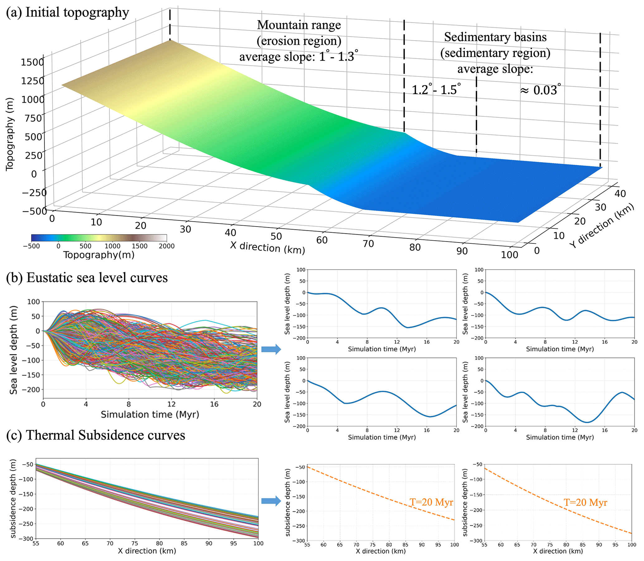
Figure 3Some examples of (a) initial topography, (b) eustatic sea level curves, and (c) thermal subsidence curves. Initial topography consists of a 55 km (x direction) by 40 km (y direction) mountain range (erosion region) and a 45 km (x direction) by 40 km (y direction) sedimentary basins (sedimentary region). The average slope of the mountain range varies from 1.0–1.3∘. Sedimentary basins contain a slope with an average slope of 1.2–1.5∘ and a basin with an average slope of about 0.03∘. The sea level curve consists of multiple sets of sinusoids whose periods are randomly set, and depths vary randomly between 50 and −200 m. The thermal subsidence curve of the sedimentary basin is determined by a distance-dependent stretching factor (McKenzie, 1978; Salles et al., 2018; Ding et al., 2019), which is randomly set to vary from 1.20–1.58.
However, the width of the initial topography should not be too narrow compared to its significantly long extension (100 km) in the x direction. Otherwise, a large amount of sediment, produced in the mountain range (erosion region), will spill out of the simulation zone during long-distance transportation to the sedimentary basin, which may result in an unstable simulation and yield unreasonable depositional hiatus in the sedimentary basin. With these considerations, we set the width of the initial topography to 40 km (y direction) to speed up the simulation process and save computational costs while ensuring the stability of the deposition simulation. By randomly choosing the parameters of the mountain range and sedimentary basin as discussed above, we generate 200 unique initial topographies, and we display one of them in Fig. 3a.
The change in sea level is a major control on the accommodation of the sedimentary basin. We randomly generate 1000 different eustatic sea level curves with a period of 20 Myr starting from 0 m, and each curve consists of multiple sets of sinusoids. The periods and amplitudes of their sinusoids are randomly set from 4–20 Myr and −200–50 m, respectively. These randomly generated sea level curves (Fig. 3b) help simulate diverse stratigraphic models with various sedimentary geometries.
Thermal subsidence can also affect the accommodation of the sedimentary basin. We use a simple subsidence model and set its corresponding parameters based on McKenzie (1978) to simulate the thermal subsidence of sedimentary basins. We also assume that the stretching factor in the model is distance-dependent (Ding et al., 2019), and we randomly set the slope of the linear relationship between the stretching factor and distance. Finally, the thermal deposition rate in the sedimentary basin is set to be about 2.48–15.0 m Myr−1 (Fig. 3c).
Rainfall patterns can affect sediment-supply changes (δS) by changing the power of river streams regarding erosion and transporting sediments to sedimentary basins. We first randomly divide the entire simulated cycle into several parts and then randomly set a spatially uniform precipitation rate (about 0.5–4 m yr−1) for each part. Moreover, in order to guarantee a stable sediment supply within the mountain range during the long-period erosion, we keep uplifting the mountain range while the simulation processes. We also predefined an initial surface porosity and then calculated the porosity distribution for each stratigraphic layer during the simulation according to the porosity–depth relationship suggested by Athy (1930). The porosity–depth relationship takes into account the mechanical compaction of the sediment, i.e., porosity gradually decreases with increasing overburden.
By using various combinations of the 200 initial topographies, 1000 eustatic sea level curves, 30 thermal subsidence curves, different rainfall patterns, etc., we simulate 1000 diverse stratigraphic models, each with multiple clinoform attribute layers such as depth, relative geologic time, porosity, and paleodepth (related to the depositional environment). Figure 4 shows 2D slices that are extracted from three of the simulated 3D models. By using the SFM discussed above, we actually simulate only the stratigraphic layers denoted by the black curves in Fig. 4 and corresponding attributes. We further use the attributes of relative geologic time, paleodepth, and porosity in conjunction with the depth curves to interpolate the corresponding full models as shown in color in each column of Fig. 4. In the following section, we discuss in detail how to build such property models and perform geophysical forward modeling to construct training datasets of seismic images and the corresponding stratigraphic labels. With the geological forward modeling process discussed above, we obtain 1000 numerous stratigraphic models of clinoform layers.
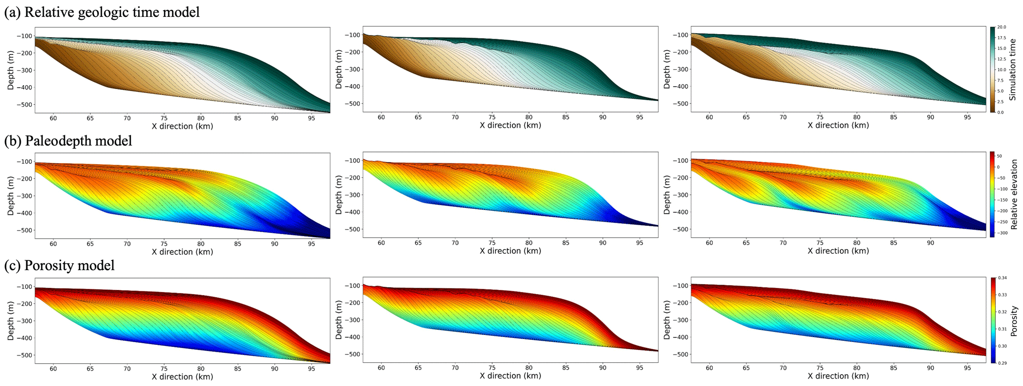
Figure 4Three 2D examples of stratigraphic models with clinoform attribute layers from stratigraphic forward modeling. (a) The relative geologic time model. (b) Paleodepth model. (c) Porosity model. The dimensions of the outputs are (X, Y, Z, N), where X and Y denote the length and width of the initial topography with a resolution of 100 m, Z represents the vertical magnitude of the stratigraphic layers in the depth direction, and N indicates the number of stratigraphic layers generated during the simulation. The black curves in the figure represent the positions of each clinoform attribute layer displayed at 4 Myr intervals. The colors in the figures represent the simulation time, paleodepth, and porosity.
2.2 Building impedance model
Before generating numerous synthetic seismic data and corresponding segmentation labels, we need to compute impedance and slope models from the porosity and depth models of clinoform layers, respectively. In this study, we use the velocity–porosity relationship model proposed by Krief et al. (1990) to build impedance models, which assumes that the velocities of P and S waves in porous fluid-saturated rocks obey Gassmann equations with the Biot compliance coefficient (Krief et al., 1990; Gassmann, 1951; Biot, 1941; Goldberg and Gurevich, 2008). To obtain an impedance model, we first calculate the formation density ρfm, shear modulus μfm, and bulk modulus Kfm by using the following equations suggested by Krief et al. (1990), Lee (2005), and Gassmann (1951):
In the formation density equation (Eq. 1), ϕ is porosity values, ρma=2.65 kg m−3 is the density of matrix material, and ρfl=1.04 kg m−3 is the density of fluid. In the formation shear modulus equation (Eq. 2), μma=13.48 GPa is the matrix material shear modulus and β is the Biot coefficient, and it is assumed that the presence of fluid has no or little influence on the shear modulus of the formation (Krief et al., 1990; Lee, 2005). The Biot coefficient β is related to the porosity and can be calculated by the following empirical relationship equations suggested by Krief et al. (1990):
In the empirical relationship equations (Eqs. 4 and 5), m(ϕ) is a function of the porosity. In the formation bulk modulus equation (Eq. 3), Kma=15.45 GPa is the matrix material bulk modulus, Kfl=2.25 GPa is the fluid bulk modulus, and M is a modulus which is dependent on the Biot coefficient and can be calculated by the following equation suggested by Gassmann (1951):
In these equations (Eqs. 1–6), some predefined parameters are taken from Carcione et al. (2002). After calculating the Kfm, ρfm, and μfm, we can calculate the velocity of P and S waves and the impedance models of P and S waves by the following equations:
where VP is the P wave velocity, VS is the S wave velocity, ZP is the P wave impedance, and ZS is the S wave impedance. At the same time, we further use the depth model of clinoform layers to calculate the slope model used to generate the segmentation label.
After calculating these stratigraphic and seismic attribute models of clinoform layers, we also need to perform the interpolation method to build corresponding 2D attribute models because the dimensions of these stratigraphic and seismic attribute models of clinoform layers are not length (x direction) and depth (z direction) but length (x direction) and the number of stratigraphic clinoform lines (n). Moreover, the resolution of the inline (x direction) direction is generally 25 m in field seismic data, but the resolution of each stratigraphic clinoform line in the inline direction (x direction) is 100 m. We first interpolate these stratigraphic and seismic attribute models of clinoform layers in inline directions (x direction) to match the resolution of field seismic data. Then we convert them (X, N) into corresponding 2D attribute models of dimension (X, Z) by interpolation in the depth direction (z direction) (see Fig. 5).
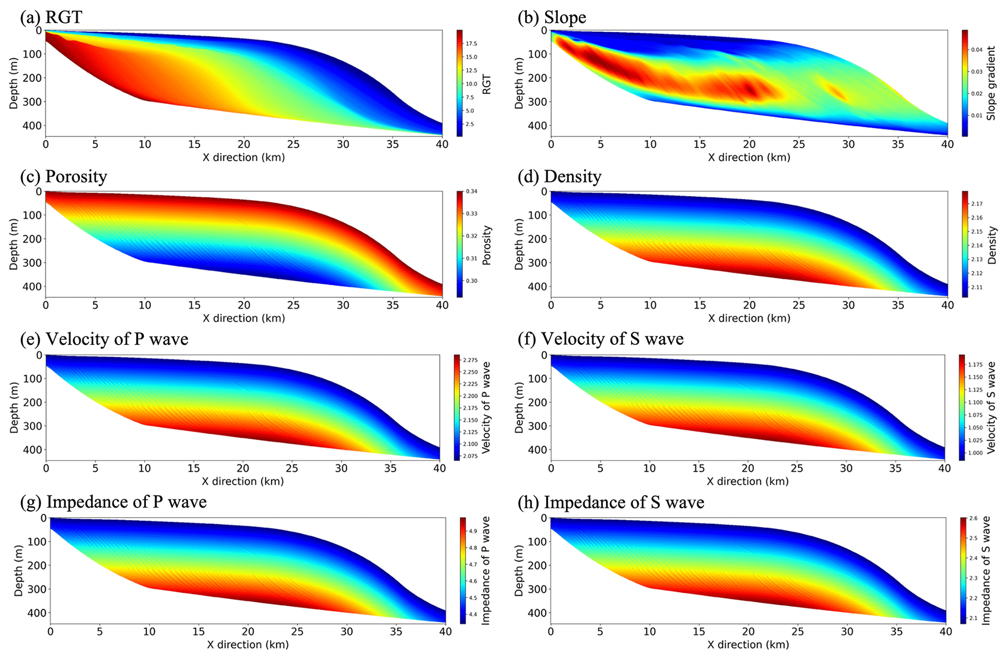
Figure 5Examples of 2D clinoform attribute models obtained by an interpolation method and velocity–porosity relationship. (a) Relative geologic time (RGT). (b) Slope. (c) Porosity. (d) Density. (e) P wave velocity. (f) S wave velocity. (g) P wave impedance. (h) S wave impedance. The dimension of the outputs is (X, Z), where X is the length of the 2D clinoform attribute model with a resolution of 25 m, and Z is the depth of the 2D clinoform attribute model with a resolution of 1 m.
2.3 Building synthetic seismic data and corresponding segmentation labels
In practice, the field seismic data are usually in the time domain. In this case, to be consistent with the field seismic data, we need to convert these 2D clinoform attribute models from the depth domain to the time domain by the depth-to-time relationship as follows:
where t[i] and t[i−1] represent two-way travel time, dz is the vertical sampling rate in the depth domain (i.e., the distance between the (i−1)th and ith samples), and vp[i] is the velocity of the P wave at the ith sample. By performing the iterative operation on each column of the 2D velocity model and resampling according to a predefined time sampling rate, we can obtain the mapping relationship from the depth domain to the time domain. Then we generate the stratigraphic and seismic attribute models of dimensions (X, T) by applying this calculated mapping relationship.
To generate the synthetic seismic data, we convolve the reflectivity model (converted from the impedance model) with a Ricker wavelet with a random peak frequency shown in Fig. 1j. The peak frequency of the Ricker wavelet is randomly chosen from a predefined range (40–60 Hz) with reference to the peak frequency extracted in the field seismic data (Tetyukhina et al., 2010). Figure 6a shows a synthetic clinoform seismic profile simulated in this way.
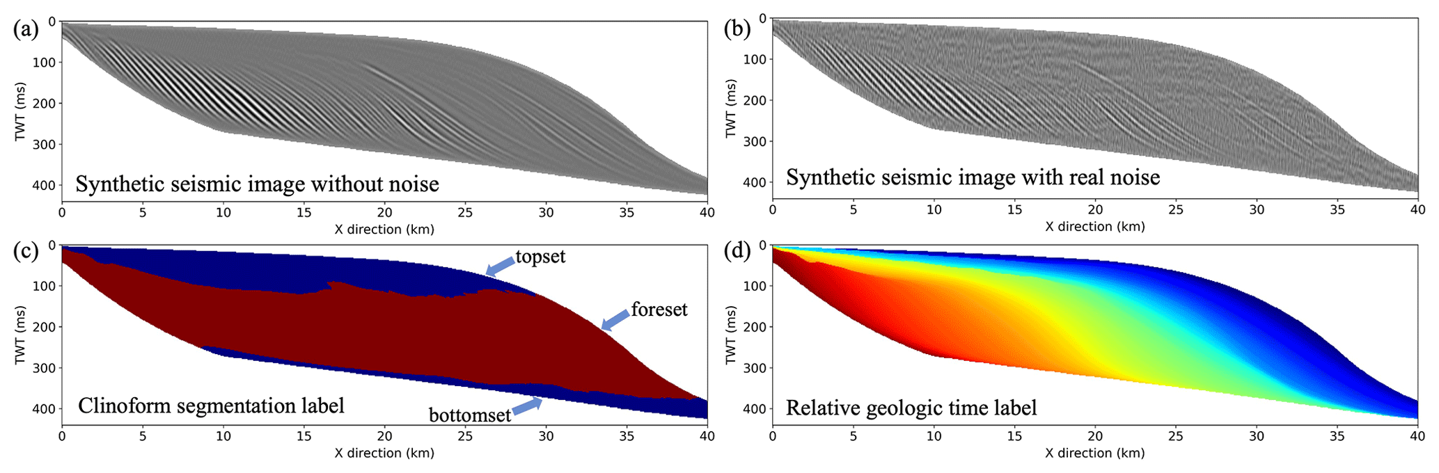
Figure 6Example of (a) synthetic seismic image without noise, (b) synthetic seismic image with noise extracted from field seismic data, (c) corresponding clinoform segmentation label, and (d) relative geologic time label. The foreset part of the clinoform is filled in red, whereas the topset and bottomset parts of the clinoform are filled in blue. The dimension of the profiles is (X, T), where X is the length of the 2D profiles with a resolution of 25 m, and T is the two-way travel time of the 2D profiles with a resolution of 2 ms.
To further improve the realism of the synthetic seismic data, we first extract the real noise from the filtered seismic data of the F3 block in the North Sea, Australia Poseidon, and Alaska North Slope data. Then we perform data augmentation on different noise data by flipping and synthesizing all the enhanced real noise data into a 3D noise volume. Finally, we add 2D real noise (with a randomly chosen slice from 3D noise volume) to the 2D seismic data according to a randomly selected signal-to-noise ratio, and we display the synthetic seismic data with real noise in Fig. 6b.
Finally, we generate the corresponding segmentation label using the slope model in the time domain. We set the region with a slope greater than 0.0175 (slope angle>1∘) as the foreset areas of the clinoform and other regions as the topset and bottomset areas of the clinoform. The threshold value of the slope refers to Pellegrini et al. (2020). The corresponding clinoform label and relative geologic time label are shown in Fig. 6c and d, respectively.
In addition, we can automatically generate numerous and diverse synthetic seismic data and the corresponding clinoform attribute models (e.g., slope model, sea level curve, relative geologic time model, and paleodepth model) based on these geological and geophysical forward modeling processes. This indicates that our workflow can be easily extended for other seismic stratigraphic interpretation tasks such as clinoform delineation, sequence boundary identification, synchronous horizon extraction, shoreline trajectory identification, and sedimentary facies analysis. In this work, we take the seismic clinoform delineation task as an example to demonstrate the effectiveness of using the synthetic dataset for training.
We consider clinoform delineation as an image segmentation problem with the goal to label ones on the foreset part of the clinoform but zeros on the topset and bottomset parts of the clinoform in 2D seismic data. In this study, we use a modified encoder–decoder deep neural network to implement the clinoform delineation. We first train the network with synthetic seismic data and corresponding segmentation labels and then use the trained network to delineate clinoform in both synthetic and field seismic data.
3.1 Network architecture
As shown in Fig. 7, the architecture of our encoder–decoder deep neural network used in this work is modified from DeepLabv3+, which was proposed by Chen et al. (2018). It has achieved state-of-the-art performance in the natural image semantic segmentation field (PASCAL VOC 2012 and Cityscapes datasets). The backbone of the DeepLabv3+ is an encoder–decoder architecture, which downscales the input images and extracts low-level semantic features and high-level semantic features in the encoder module and gradually recovers sharp boundaries in the decoder module (Ronneberger et al., 2015; Badrinarayanan et al., 2017; Chen et al., 2018). However, compared to the original DeepLabv3+, we remove the skip connections between the encoder and decoder layers because we found that the low-level features from the encoder layers lead to some artifacts in the predicted results.
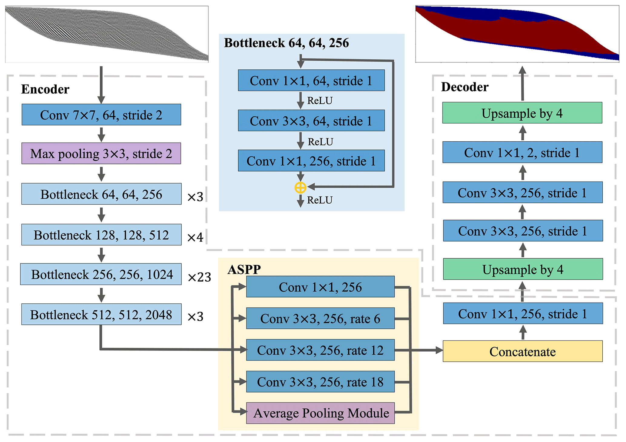
Figure 7The architecture of the network for clinoform delineation. The left dashed gray box is the encoder module which consists of a ResNet-101 and an ASPP module. The blue box in the middle is the module of ResBlocks in the encoder, which contains a 1×1 convolutional layer, a 3×3 convolutional layer, a 1×1 convolutional layer, and a skip connection. The orange box in the middle is the module of ASPP in the encoder, which contains a 1×1 convolutional layer; three 3×3 atrous convolutional layers with sampling strides of 6, 12, and 18; and an average pooling module. The right dashed gray box is the encoder module which consists of an upsampling layer, two 3×3 convolutional layers, a 1×1 convolutional layer, and an upsampling layer.
In the modified network, the encoder module (see left dashed gray box in Fig. 7) consists of a deep convolutional neural network (DCNN) and an atrous spatial pyramid pooling (ASPP) module. The DCNN module consists of a ResNet-101 (He et al., 2016) and is used to progressively reduce the resolution of feature maps and capture high-level semantic features. ResNet-101 consists of a 7×7 convolutional layer with a stride of 2, a 3×3 max pooling with a stride of 2, and four ResBlocks. These four ResBlocks are composed of bottleneck blocks with numbers of 3, 4, 23, and 4 and strides of 1, 2, 1, and 1, respectively. The bottleneck block consists of a 1×1 convolutional layer, a 3×3 convolutional layer, a 1×1 convolutional layer, and a skip connection (see blue box in Fig. 7). The ASPP module can capture the contextual information at multiple scales, which are composed of a 1×1 convolutional layer; three 3×3 atrous convolutional layers with sampling strides of 6, 12, and 18; and an average pooling module (see the orange box in Fig. 7).
The decoder module in the modified networks (see right dashed gray box in Fig. 7) first uses a bilinear upsampling layer to upsample the high-level semantic features by a factor of 4, and then the upsampled features are fed to two 3×3 convolutional layers and a 1×1 convolutional layer which obtains the probabilities of each class and reduces the channels of features to the number of classes. Finally, the same bilinear upsampling layer is applied to obtain the final feature maps of the same size as the input image. These final feature maps are fed to a softmax layer and an argmax layer to obtain the final clinoform segmentation result.
3.2 Training and validation
After automatically generating 1000 pairs of synthetic seismic data (Fig. 6b) and corresponding clinoform labels (Fig. 6c), we train and validate our CNN model by using 800 and 200 pairs of them, respectively. Considering the amplitude values of field seismic data can vary widely, we perform a normalization process to each seismic dataset before feeding it into the CNN model by subtracting its mean value and then dividing by its standard deviation.
Considering clinoform delineation in the 2D seismic image is a binary segmentation problem, we use the following binary cross entropy loss function ℒ to train our network:
where N denotes the number of pixels in the input 2D seismic data, and xi and yi represent the prediction and label at the ith pixel, respectively.
In the training of the network, the size of each synthetic seismic dataset and corresponding segmentation label is 1600×256 pixels. Considering the computation time and memory, we feed the normalized synthetic seismic images and corresponding segmentation labels to the CNN in batches and set the batch size to 16. We use the Adam optimizer (Kingma and Ba, 2014) to optimize the network parameters. In the training process, we start the learning rate at 0.01 and adaptively reduce it based on the validation loss. Specifically, we automatically reduce the learning rate by half when the validation metric stagnates within 2 epochs. In total, we use 800 and 200 pairs of synthetic training datasets to train and validate our CNN model. As shown in Fig. 8, the curves for both training (blue curve) and validation (orange curve) losses converge to 0.02 and 0.08, while the learning rate decreases to 0.00001 after 200 epochs.
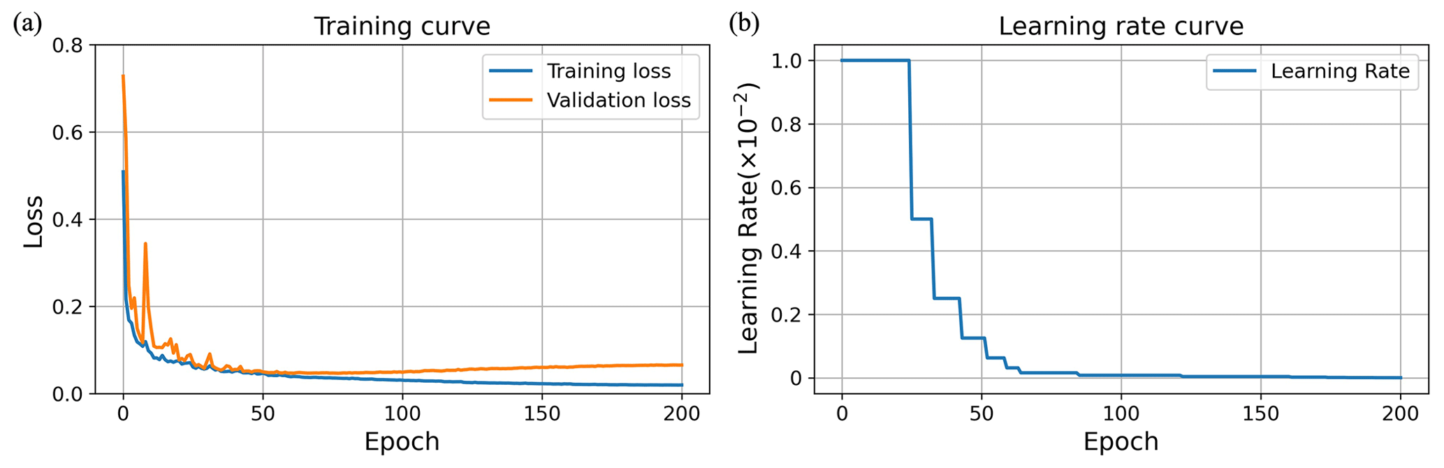
Figure 8(a) The loss curves of training (blue) and validation (orange). (b) The learning rate is adaptively adjusted in the training process. The curves for both training (blue curve) and validation (orange curve) losses converge to 0.02 and 0.06, whereas the learning rate decreases to 0.00001 after 200 epochs.
To demonstrate the performance of the trained network, we first apply it to six synthetic seismic images with classic clinoforms (Fig. 9c) that are generated by six classic sea level curves with 1, 1.5, and 2 sinusoidal periods as shown in Fig. 9a. Note that real noise extracted from field seismic data has been added to the synthetic seismic data (Fig. 9c). By feeding the synthetic seismic data to our trained network, we obtain the clinoform segmentation results shown in Fig. 9e. We observe that the segmentation results are consistent with the ground truth labels shown in Fig. 9d. It is not surprising that the trained network works well in these synthetic seismic data simulated by using the same workflow of generating the training dataset. We therefore further validate our network in multiple field seismic data in the following sections.
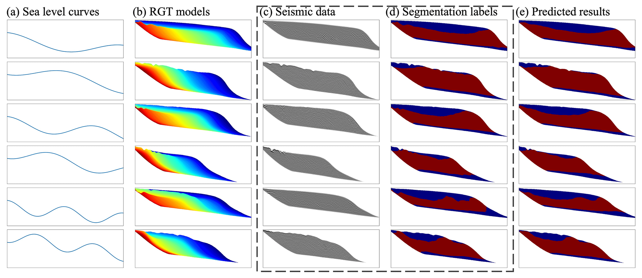
Figure 9Examples of (a) classic sea level curves with 1, 1.5, and 2 cycles; (b) relative geologic time (RGT) model; (c) synthetic seismic image with real noise; (d) corresponding segmentation labels; and (e) predicted results using the trained network. The foreset part of the clinoform is filled in red, whereas the topset and bottomset parts of the clinoform are filled in blue. From the predicted results, we can find that (e) the predicted results are consistent with (d) the labels, which means the network has successfully learned to extract the structural features for clinoform segmentation in the seismic images.
3.3 Eliminating outliers by smoothing feature maps
We further verify the performance of our trained network on a field seismic data with more complex features as shown in Fig. 10a. Figure 10b shows the predicted result, where red and blue represent the foreset part and topset or bottomset parts of the clinoform, respectively. We observe that most of the foreset areas are correctly predicted, but the areas indicated by the cyan arrows are incorrectly predicted as the topset or bottomset of the clinoform, and the area indicated by the green arrow is incorrectly predicted as the foreset part of the clinoform.

Figure 10We input (a) a field seismic profile into the trained network and get (b) the corresponding predicted result, where red represents the foreset part of the clinoform and blue represents the topset and bottomset parts of the clinoform. The clinoform segmentation result is mostly correct, but we also observe some holes and outliers as indicated by cyan and green arrows in (b), respectively. To further fill the holes and eliminate the outliers, we introduce structural smoothing layers into the network to enhance the feature maps of the network and therefore obtain a cleaner and more complete result in (c).
To better understand the feature extraction and prediction process of the network in segmenting a clinoform, we display the feature maps of each layer in the network in Fig. 11. The encoder module in the networks (see the left part in Fig. 11) focuses on extracting features of the foreset part of the clinoform, topset or bottomset parts of the clinoform, and boundaries. The decoder module in the network (see the right part in Fig. 11) focuses on gradually recovering the specific areas of the foreset part of the clinoform and topset or bottomset parts of the clinoform according to the features extracted by the encoder module. We expect that the foreset part of the clinoform should be a complete and continuous block; however, the predicted result shown in Fig. 10b obviously does not conform to such a priori geological understanding.
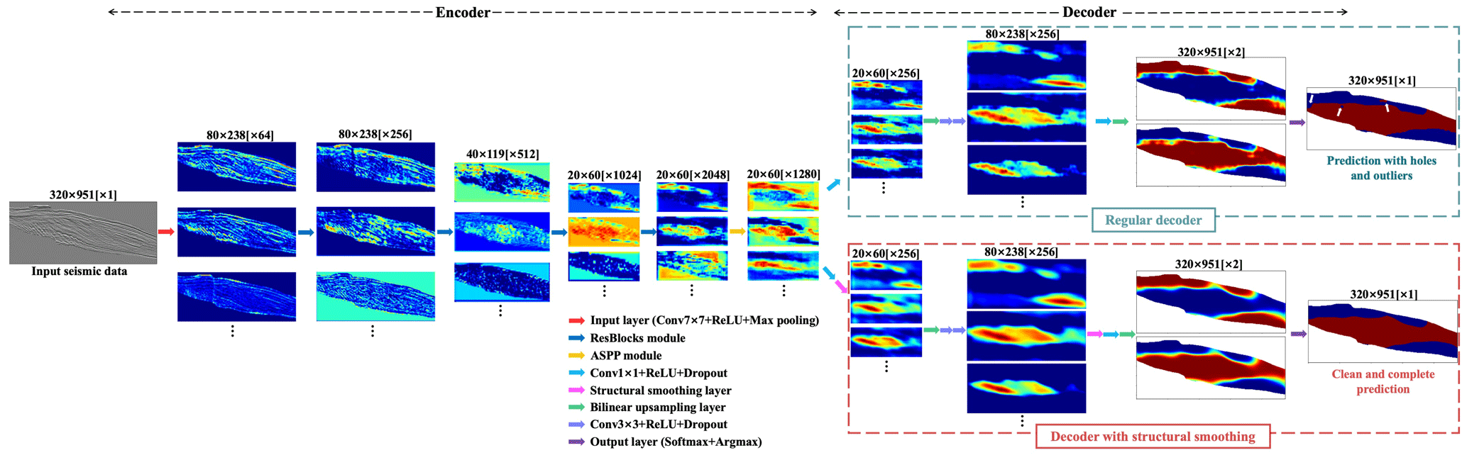
Figure 11The feature maps of the encoder–decoder networks. The red arrow denotes an input layer containing a 7×7 convolutional layer with ReLU and a max-pooling layer. The navy blue arrow denotes four different ResBlocks modules consisting of bottleneck blocks with numbers of 3, 4, 23, and 4 and strides of 1, 2, 1, and 1, respectively. The yellow arrow denotes the ASPP modules. The light blue arrow denotes a 1×1 convolution layer with ReLU and dropout. The pink arrow denotes structural smoothing layers at or scale. The green arrow denotes a bilinear upsampling layer. The light purple arrow denotes a 3×3 convolution layer with ReLU and dropout. The navy purple arrow denotes an output layer consisting of a softmax layer and an argmax layer. The upper right dashed green box and lower right dashed red box refer to the feature maps and predicted results before and after the introduction of the structural smoothing layer, respectively.
In order to make the segmentation results of the trained network on the field seismic data more clean and complete, we incorporate a preconditioning layer (Wu et al., 2023) of structure-oriented smoothing into the network. This smoothing layer enhances the structural features along the seismic structural orientations, thus filling holes and eliminating outliers in the final segmentation results. We first estimate the structural orientation at each pixel of the input seismic image by using the method of structure tensor (Van Vliet and Verbeek, 1995; Fehmers and Höcker, 2003; Hale, 2009). Then we construct the corresponding smooth convolution kernels along the seismic structures based on the estimated orientations. Finally, we apply these structure-oriented smoothing kernels to the feature maps at the scales of and in the network, as denoted by pink arrows in Fig. 11.
After introducing the structural smoothing layer into the network, the predicted results shown in Fig. 10c are more complete and continuous. To visually demonstrate the function of the introduced structural smoothing layers, we display the feature maps of the decoder module after introducing the structure-oriented smoothing layers in the dashed red box in Fig. 11. Compared to the original decoder module in the dashed green box, the feature maps with the smoothing layers become cleaner and more continuous for the features of topset, foreset, and bottomset of the clinoform, and the predicted result based on these feature maps is therefore cleaner and more complete.
In addition to the synthetic seismic data, we also use three different field seismic datasets to verify the performance of the network trained with only synthetic seismic data. In our simulated synthetic training datasets, the seismic images (like the one in Fig. 6b) contain only the simulated processes of the clinoform deposition with dramatic changes in sea level but do not contain the non-clinoform part with horizontal deposition. However, the field seismic images typically contain a large number of horizontal deposits, and the clinoform deposits are only a small part of them. In order to be consistent with the training datasets, we first use an automatic horizon-picking method proposed by Wu and Fomel (2018) to extract the top and bottom layers of the part of the clinoform deposition in the field seismic data. Then we cut out the sub-volume with the clinoform deposits from the whole seismic volume by using the two computed boundary layers. To avoid the uncertainty of the seismic amplitude variation range of the field survey seismic data, each of them is first subtracted by its mean and then divided by its standard deviation to obtain a normalized seismic dataset.
4.1 Case study one: Netherlands offshore F3 Block
The first field example is the Netherlands offshore F3 Block (Dutch sector) seismic data acquired in the northeastern part of the North Sea. In this survey, a large fluvio-deltaic system dominated the basin resulting in a massive clinoform deposition during the Cenozoic era (Tetyukhina et al., 2010). The survey area of this seismic volume is 24 km in the inline direction, 16 km in the crossline direction, and 1848 ms in the two-way travel time direction. In this work, we select a 3D subset (951 (inline) × 460 (crossline) × 320 (time) samples) of F3 Block seismic data as the study seismic volume (Fig. 12a).
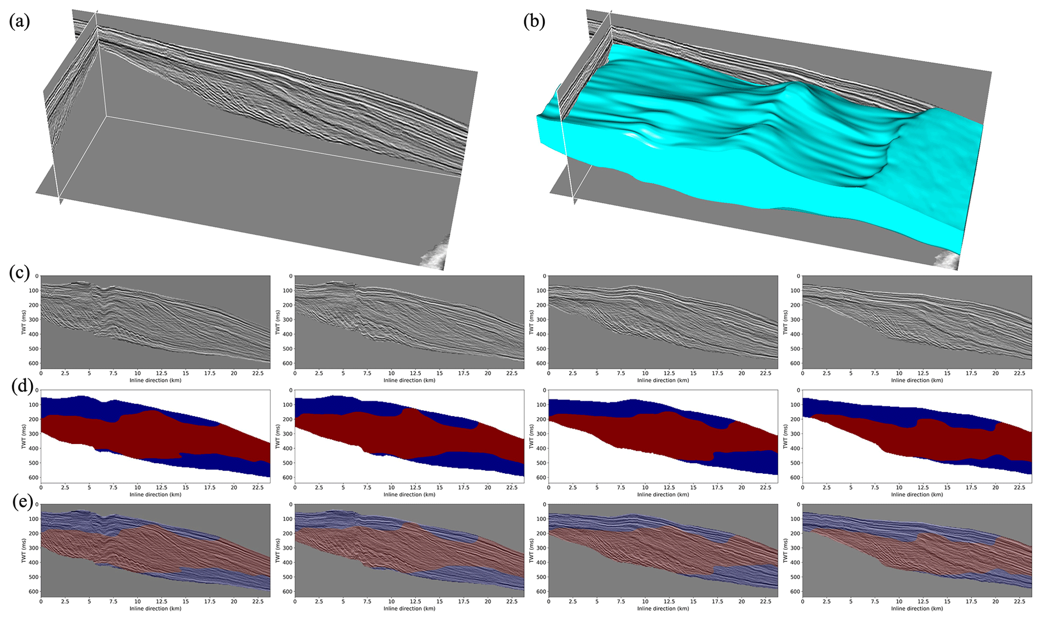
Figure 12Case study one: Netherlands offshore F3 Block seismic data. (a) The 3D subset of the F3 Block seismic data, (b) 3D body of the foreset area of the predicted clinoform, (c) four 2D seismic profiles extracted from the 3D seismic volume, (d) the predicted results using the network trained with only synthetic clinoform seismic data, and (e) the results overlaid with the seismic profiles. The foreset areas of the clinoform in 2D profiles are filled with red, whereas the topset and bottomset areas of the clinoform are filled with blue. From the predicted results, the topset, foreset, and bottomset parts of the clinoform can remain clean and complete, and the boundaries between the topset and foreset and between the foreset and bottomset can maintain continuity.
We first use the method proposed by Wu and Fomel (2018) to extract the top and bottom surfaces of the part of the clinoform deposition in this seismic volume and then cut the sub-volume (Fig. 12a) between the two surfaces. We then apply the trained network to delineate the clinoform in the 3D sub-volume slice by slice in the crossline direction. Each 2D slice (951 (inline) × 320 (time) samples) is normalized by its mean and standard deviation before being fed into the network. In these seismic images, some complex geological structures, such as faults with large fault throws and uplifts of salt bodies, bring challenges for the clinoform delineation. We further introduce the structural smoothing layer at scale on the decoder module to enhance the structural features along the seismic structural orientations, thus filling holes and eliminating outliers in the final segmentation results.
Figure 12c shows some 2D seismic slices that are extracted from the 3D seismic volume, and Fig. 12d displays the corresponding clinoform segmentation results. The red regions represent the foreset areas of the clinoform predicted by the trained network, whereas the blue regions represent the topset or bottomset areas of the clinoform. In order to intuitively evaluate the predicted results, we also display the results by overlaying the predicted results with the seismic images shown in Fig. 12e. To visualize the predicted results for the entire 3D volume, we also use the classic marching cubes algorithm proposed by Lorensen and Cline (1987) to extract a 3D foreset equivalence surface as shown in Fig. 12b, where the foreset areas of the clinoform are displayed as a 3D geobody with cyan color.
As is shown in Fig. 12b, d, and e, the prediction segmentation results can maintain high integrity and continuity and separate the foreset, topset, and bottomset of the clinoform in seismic profiles, which demonstrates the reliable generalization of the trained network in this field data example. From the seismic images (Fig. 12c), they are complicated by some special structural features, such as faults with large fault throws, uplifts of salt bodies, and fold deformation, which are not included in the training datasets. However, our prediction results are generally not affected by these special features. This indicates that the trained network has successfully learned to analyze the geological structure information of the topset, foreset, and bottomset parts of the clinoform from a global perspective, not just from the local characteristics of seismic data. Moreover, it shows that the trained network has certain anti-noise ability and generalization for some complex structures.
4.2 Case study two: Australia Poseidon seismic data
The second field example is the Poseidon 3D seismic volume acquired in the Browse Basin's shelf margin, northwestern Australia (Liu, 2018; Dixit and Mandal, 2020). The survey area of this seismic volume is 64 km in the inline direction, 63 km in the crossline direction, and 6000 ms in the two-way travel time direction. The grid size of this 3D seismic volume is 18.75 m (inline) × 12.5 m (crossline) × 4 ms (time). We first resample this 3D seismic volume and then select a 3D subset (618 (inline) × 288 (crossline) × 192 (time) samples) of the Australia Poseidon 3D seismic volume as the study seismic volume.
We first extract the top and bottom surfaces of the part of the clinoform deposition in the 3D seismic volume. Then we flatten the 3D seismic volume with the top surface as a horizontal datum to eliminate the tectonic influence of the overlying strata. After flattening the 3D seismic volume, we cut the flattened seismic volume (Fig. 13a) between the two surfaces to preserve the clinoform deposits and remove the non-clinoform deposits. After these processes, we fed the 3D sub-volume slice by slice in the y direction into the trained network to delineate the clinoform. To be consistent with the synthetic seismic data, each 2D slice (618 (inline) × 192 (time) samples) is normalized before being fed into the network. Similar to study case one, we also introduce the structural smoothing layer in the decoder module of the network to enhance the features maps along the seismic structural orientations.
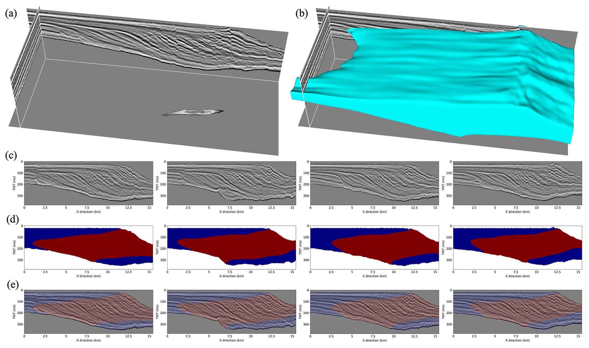
Figure 13Case study two: Australia Poseidon 3D seismic data. (a) The flattened 3D subset of Australia Poseidon seismic data, (b) the 3D body of the foreset area of the predicted clinoform, (c) four randomly selected 2D seismic images, (d) the predicted results using the trained network, and (e) the results overlaid with the seismic images. The foreset areas of the clinoform in 2D profiles are filled with red, whereas the topset and bottomset areas of the clinoform in 2D profiles are filled with blue.
We randomly select four 2D seismic slices (Fig. 13c) from the 3D seismic sub-volume and display the corresponding clinoform segmentation results in Fig. 13d. The red and blue regions represent the foreset areas of the clinoform and topset or bottomset areas of the clinoform predicted by the trained network, respectively. We also overlay the predicted results with seismic images shown in Fig. 13e and display a 3D view of the segmented clinoform body in Fig. 13b. As shown in Fig. 13b, d, and e, the predicted results are clean and complete, where the topset, foreset, and bottomset areas of the clinoform are mostly reasonably segmented.
4.3 Case study three: Alaska North Slope
Data for the third field seismic case study are acquired at the Alaska North Slope, which is a well-known Lower Cretaceous clinoform depositional sequence. It is also a large depositional-scale (600–1000 m depositional thickness in the north and 1700–2000 m depositional thickness in the south) constructional siliciclastic clinoform (Bird and Molenaar, 1992; Houseknecht et al., 2009; Ramon-Duenas et al., 2018). This study includes three publicly available 2D seismic profiles (from 1974–1981) from the United States Geological Survey (USGS), which are 58-75 trackline, 28-81 trackline, and 39-81 trackline, respectively. We select 110 km (inline) × 1800 ms (time), 55 km (inline) × 800 ms (time), and 50 km (inline) × 800 ms (time) 2D seismic sub-profiles, respectively.
We extract the top and bottom layers of the part of the clinoform deposition and another top layer of the part of a horizontal deposition in each seismic profile. Then we cut out each sub-profile between the exacted top and bottom layers and flatten it based on another top layer. We further perform gain and filtering operations on the flattened seismic images to enhance the seismic features, and the processed images are shown in the left column of Fig. 14. In segmenting clinoform in these seismic profiles, the low signal-to-noise ratio of the data and the existence of complex geological structures such as faults with large fault throws and fold deformation bring great challenges to the network trained with only synthetic data. To reduce the impact of these complex structures on clinoform delineation, we introduce the structural smoothing layer to enhance the structural features along the seismic structural orientations.
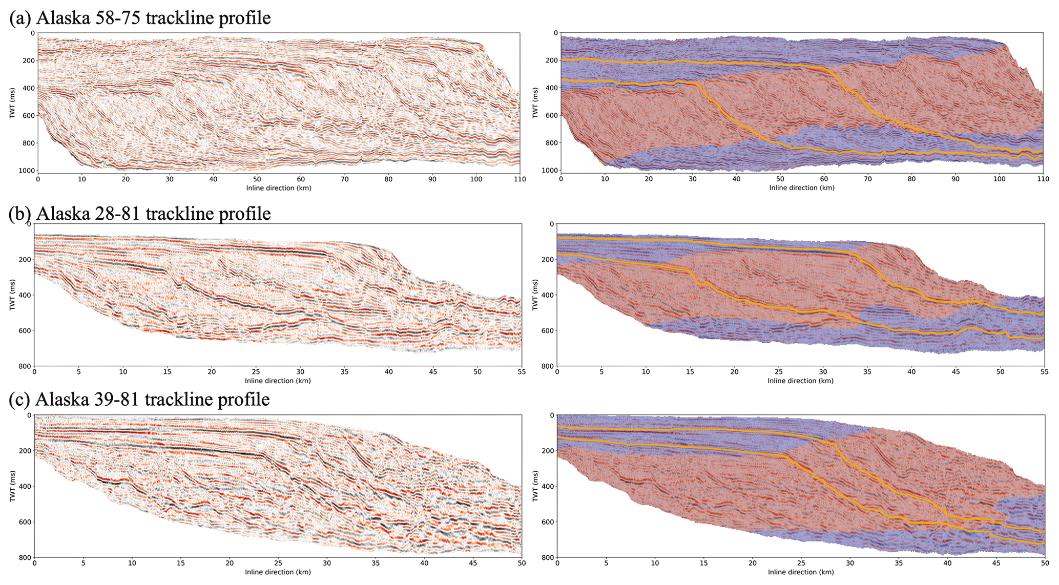
Figure 14Case study three: Alaska North Slope 2D seismic data. (a) The 58-75 trackline sub-profile and predicted result. (b) The 28-81 trackline sub-profile and predicted result. (c) The 39-81 trackline sub-profile and predicted result. The survey area of these three seismic profiles are 110, 55, and 50 km in the inline direction and 1000, 800, and 800 ms in the two-way travel time direction, respectively. The seismic profiles shown in the left column are processed by flattening, gain, filtering, and normalization operations, and the segmentation results are displayed in the right column, where the foreset areas of clinoform are filled with red and the topset and bottomset areas of clinoform are filled with blue. We also display two synchronous horizons extracted in each seismic profile with orange lines.
As shown in the right column of Fig. 14, the segmentation results predicted by our modified network are clean and complete. Comparing the predicted result (Fig. 14a) with the human interpretation result (Ramon-Duenas et al., 2018), we find that the predicted result is roughly close to the human interpretation result, particularly in the boundary between the topset and foreset. To further validate the segmentation results, we extract two synchronous horizons in each seismic profile and display them with orange lines in the right column of Fig. 14. Combining synchronous horizon distribution and segmentation results, our network can successfully segment regions with sharp slope angles on the synchronous horizons. It is indicated that our network can learn to analyze the structural features of the clinoform and can automatically segment regions with sharp slope angles (foreset regions). Moreover, the introduction of the smoothing structural layer enables the network to enhance the features and reduce the generation of holes or outliers caused by the complex structures and low signal-to-noise ratio of the data.
Applications on the synthetic data and three different field seismic data points indicate that our training datasets generated by geological and geophysical forward modeling are geologically reasonable to train our network for accurate clinoform delineation. The introduction of the structural smoothing layer at different scales enables the trained network to enhance the structural features along the seismic structural orientations in complex field seismic data applications, thus filling holes and eliminating outliers in the final segmentation results. From the segmentation results of field seismic data, the topset, foreset, and bottomset areas of the clinoform are accurately segmented into different classes, and each class maintains high integrity and continuity.
Although the segmentation results are visually reasonable in general, some artifacts or inaccurate predictions still appear in some local areas of the results, which indicates some limitations of our method. The main limitation remains in the workflow of generating synthetic training datasets by geological and geophysical forward modeling. We use a specific modeling engine (pyBadlands) for stratigraphic forward modeling, which offers several advantages over alternative models. Specifically, pyBadlands is open-source, source-to-sink, and comprehensive in its consideration of influencing factors, and it can effectively simulate diverse datasets (Salles and Hardiman, 2016; Salles et al., 2018; Ding et al., 2019). However, it is important to note that pyBadlands is only capable of numerical simulation and cannot fully replicate natural surface processes. For instance, the porosity model generated by SFM models only considers the mechanical compaction of the sediment, which may result in less realism in the synthetic seismic data. Moreover, we have not yet included any folding and faulting structures, salt bodies, or channels in generating the stratigraphic layers and the corresponding seismic data. These structure features, however, may significantly affect the seismic stratigraphic interpretation tasks. In this paper, we have flattened the seismic data to remove the folding and faulting structures before the clinoform segmentation, which makes the data structurally more consistent with the training seismic data and therefore reduces the segmentation challenges due to various structures. In the future, we need to build more realistic stratigraphic models with various structural patterns and geobodies to better train a network for interpreting more complex seismic data. Additionally, note that here we only consider the slope information when generating the clinoform segmentation labels, which could lead to some inaccuracies in the labeling process.
In terms of network selection, we select U-net, DeeplabV3+, and DeeplabV3+ without a skip connection for the comparison test. We train these networks using the cross entropy (CE), mean squared error (MSE), binary cross entropy (BCE), and binary cross entropy with log (BCEWithLogits) loss functions, respectively. These network tests show that the DeeplabV3+ network without skip connection using cross-entropy loss function is the most stable and accurate in both synthetic and field seismic data applications. In addition to the network architectures and loss functions, the size of the seismic data or the scale of the clinoform is another important aspect affecting the segmentation results. For example, the training dataset with a scale size of 1600×256 pixels performed well on the large-scale Alaska North Slope data but performed poorly on the small-scale F3 Block and Australia Poseidon seismic data. Therefore, we also simulated small-scale clinoform training datasets with a scale size of 900×256 pixels for F3 Block and Australia Poseidon seismic data and obtained stable and accurate segmentation results by the trained network.
In practice, the quality of the field seismic data may not be as high as synthetic data because of noise, seismic migration artifacts, and unclearly imaged reflections. We have added noise, extracted from field seismic data, to the synthetic data to train our network. However, the network may still generate holes and outliers in delineating clinoform in poor-quality seismic data. Based on the prior geologic knowledge that each part (topset, foreset, and bottomset) of the clinoform segmentation should be a complete and continuous block, we introduce the structural smoothing layer to our network. The structure-oriented convolution kernels in the smoothing layer smooth the feature maps computed in the network along the seismic structure orientations to suppress noisy features while enhancing the continuity of effective features in the maps, thus filling holes and eliminating outliers in the final segmentation results. Moreover, the structural smoothing layer can be integrated into the network at different scales. This means that the structural smoothing layer is highly scalable and can be introduced at any depth of the network.
Considering the computational cost, the synthetic training datasets used for network training are 2D, and the initial topography used for the stratigraphic forward modeling is a simple slope surface with lateral consistency. In the future, we can upgrade our workflow from 2D to 3D by designing more complex and extensive initial topographies to generate diverse 3D clinoform seismic datasets. Additionally, we can take into account some other factors in building the porosity model to enhance its diversity and realism. For example, we can introduce the constraints of the paleodepth model based on the sorting effect of the ocean on sediments, and we can also introduce the constraints of the natural variability in rock properties according to the initial variations in provenance. The introduction of these multiple constraints can improve the diversity of the porosity model, enhance the realism of the synthetic data, and improve the process of the stratigraphic forward modeling. Additionally, for the generation of the slope model, we can calculate the slope model using real-time stratigraphic depth layers instead of the final depth model, which can better reflect the actual slope when sediments are deposited. In the validation stage of the field seismic data, we can further introduce some other geophysical data information (e.g., log data) to better validate the segmentation results of field seismic data. Moreover, although we only use such a workflow to solve the clinoform delineation problem at present, we can easily extend this workflow for more geological and geophysical scenarios in the future, such as sequence boundary identification, synchronous horizon extraction, relative geologic time estimation, sedimentary facies analysis, unconformity, and identification.
We propose a workflow to automatically generate synthetic seismic data of clinoform and corresponding clinoform labels. In this workflow, we employ stratigraphic forward modeling to obtain numerous stratigraphic models with clinoform layers by randomly but properly choosing initial topographies, sea level curves, thermal subsidences, and rainfall patterns. Then we convert the simulated stratigraphic model into the impedance model by using a velocity–porosity relationship while calculating the slope model from the corresponding depth model of clinoform layers. We further perform depth-to-time conversion to the impedance model, convolve it with a Ricker wavelet with a random peak frequency, and add real noise to generate a synthetic seismic image. Finally, we obtain the corresponding clinoform label according to a slope threshold. In this way, we automatically generate 1000 large-scale and 2000 small-scale synthetic seismic data and corresponding stratigraphic labels, and we make these datasets available to the public.
We use an encoder–decoder network modified from DeepLabV3+ to perform clinoform delineation. In the modified network, the encoder module consists of DCNN and ASPP modules, which are mainly used to extract features at different resolutions, and the decoder module consists of a few simple convolutional and upsampling layers, which are mainly used to refine the segmentation results. Considering the complex geological structures of the field seismic data, we introduce the structural smoothing layer in the decoder module to enhance the structural features along the seismic structural orientations, thus filling holes and eliminating outliers in the final segmentation results.
We train the modified network with only synthetic seismic datasets and then validate its performance on both synthetic and field seismic data. The segmentation results are clean, continuous, and visually reasonable. This indicates that the proposed workflow of using synthetic seismic data to train the network and using the trained network for automatic and fast clinoform delineation is plausible. Moreover, our workflow can obtain other stratigraphic labels (in addition to clinoform labels) during the geological and geophysical forward modeling. Therefore, our workflow can be easily extended for other seismic stratigraphic interpretation tasks such as sequence boundary identification, synchronous horizon extraction, shoreline trajectory identification, and sedimentary facies analysis.
The synthetic seismic datasets used for training and validating our network have been uploaded to Zenodo and are freely available at https://doi.org/10.5281/zenodo.7122471 (Gao et al., 2022b). The source codes for the geological and geophysical forward modeling and the neural network have been uploaded to Zenodo and are freely available at https://doi.org/10.5281/zenodo.7123934 (Gao et al., 2022a).
XW initiated the idea of geological and geophysical forward modeling and advised the research on it. JZ and XW initiated the idea of deep learning for seismic clinoform delineation and advised the research on it. HG conducted the research and implemented the geological and geophysical forward modeling algorithms. ZB and HG tested and modified the code for the neural network in PyTorch. HG prepared the training dataset and carried out the experiments for both synthetic and field seismic data. XW initiated the idea of introducing the structure-oriented smoothing layer in the network. XW, JZ, and XS advised on the simulation process and result analysis from a geological perspective. HG and XW prepared the paper, with contributions from all co-authors.
The contact author has declared that none of the authors has any competing interests.
Publisher's note: Copernicus Publications remains neutral with regard to jurisdictional claims in published maps and institutional affiliations.
The numerical calculations in this paper have been done on the supercomputing system in the Supercomputing Center of University of Science and Technology of China. We sincerely appreciate the constructive and thoughtful suggestions from reviewers Xuesong Ding and Mark Jessell and editor Lutz Gross on this paper.
This research has been supported by the National Natural Science Foundation of China (grant nos. 41974121 and 42050104).
This paper was edited by Lutz Gross and reviewed by Xuesong Ding and Mark Jessell.
Adams, E. W. and Schlager, W.: Basic types of submarine slope curvature, J. Sediment. Res., 70, 814–828, https://doi.org/10.1306/2DC4093A-0E47-11D7-8643000102C1865D, 2000. a
Araya-Polo, M., Jennings, J., Adler, A., and Dahlke, T.: Deep-learning tomography, The Leading Edge, 37, 58–66, 2018. a
Asquith, D.: Depositional topography and major marine environments, Late Cretaceous, Wyoming, AAPG Bull., 54, 1184–1224, 1970. a
Athy, L. F.: Density, porosity, and compaction of sedimentary rocks, AAPG Bull., 14, 1–24, 1930. a
Badrinarayanan, V., Kendall, A., and Cipolla, R.: Segnet: A deep convolutional encoder-decoder architecture for image segmentation, IEEE T. Pattern Anal., 39, 2481–2495, 2017. a, b
Bates, C. C.: Rational theory of delta formation, AAPG Bull., 37, 2119–2162, 1953. a
Bergen, K., Johnson, P., De Hoop, M., and Beroza, G.: Machine learning for data-driven discovery in solid earth geoscience, Science, 363, eaau0323, https://doi.org/10.1126/science.aau0323, 2019. a
Biot, M. A.: General theory of three-dimensional consolidation, J. Appl. Phys., 12, 155–164, 1941. a
Bird, K. J. and Molenaar, C. M.: The North Slope Foreland Basin, Alaska, American Association of Petroleum Geologists, 363–393, https://doi.org/10.1306/M55563C14, 1992. a
Burgess, P. M., Roberts, D., and Bally, A.: A brief review of developments in stratigraphic forward modelling, 2000–2009, Regional Geology and Tectonics: Principles of Geologic Analysis, 1, 379–404, 2012. a, b, c
Carcione, J. M., Helle, H. B., and Hydro, N.: Rock physics of geopressure and prediction of abnormal pore fluid pressures using seismic data, CSEG Recorder, 27, 8–32, 2002. a
Chen, L.-C., Zhu, Y., Papandreou, G., Schroff, F., and Adam, H.: Encoder-decoder with atrous separable convolution for semantic image segmentation, in: Proceedings of the European conference on computer vision (ECCV), Munich, Germany, 8–14 September 2018, 801–818, 2018. a, b, c, d
Cummings, D. I. and Arnott, R. W. C.: Growth-faulted shelf-margin deltas: a new (but old) play type, offshore Nova Scotia, Bull. Can. Petrol. Geol., 53, 211–236, 2005. a
Di, H., Shafiq, M., and AlRegib, G.: Patch-level MLP classification for improved fault detection, in: SEG Technical Program Expanded Abstracts 2018, Society of Exploration Geophysicists, 2211–2215, https://doi.org/10.1190/segam2018-2996921.1, 2018. a
Di, H., Li, Z., Maniar, H., and Abubakar, A.: Seismic stratigraphy interpretation by deep convolutional neural networks: A semisupervised workflow, Geophysics, 85, WA77–WA86, 2020. a
Ding, X., Salles, T., Flament, N., and Rey, P.: Quantitative stratigraphic analysis in a source-to-sink numerical framework, Geosci. Model Dev., 12, 2571–2585, https://doi.org/10.5194/gmd-12-2571-2019, 2019. a, b, c, d
Dixit, A. and Mandal, A.: Detection of gas chimney and its linkage with deep-seated reservoir in poseidon, NW shelf, Australia from 3D seismic data using multi-attribute analysis and artificial neural network approach, J. Nat. Gas Sci. Eng., 83, 103586, https://doi.org/10.1016/j.jngse.2020.103586, 2020. a
Fehmers, G. C. and Höcker, C. F.: Fast structural interpretation with structure-oriented filtering, Geophysics, 68, 1286–1293, 2003. a
Gao, H., Wu, X., Zhang, J., Sun, X., and Bi, Z.: huigcig/ClinoformNet: ClinoformNet-1.0, Zenodo [code], https://doi.org/10.5281/zenodo.7123934, 2022a. a
Gao, H., Wu, X., Zhang, J., Sun, X., and Bi, Z.: The synthetic and field siesmic datasets for “ClinoformNet-1.0: stratigraphic forward modeling and deep learning for seismic clinoform delineation”, Zenodo [data set], https://doi.org/10.5281/zenodo.7122471, 2022b. a
Gassmann, F.: Über die Elastizität poröser Medien, Vierteljahrsschrift der Naturforschenden Gesellschaft in Zürich, 96, 1–23, 1951. a, b, c
Goldberg, I. and Gurevich, B.: A semi-empirical velocity-porosity-clay model for petrophysical interpretation of P- and S-velocities [Link], Geophys. Prospect., 46, 271–285, 2008. a
Guo, J., Li, Y., Jessell, M. W., Giraud, J., Li, C., Wu, L., Li, F., and Liu, S.: 3D geological structure inversion from Noddy-generated magnetic data using deep learning methods, Comput. Geosci., 149, 104701, https://doi.org/10.1016/j.cageo.2021.104701, 2021. a
Hale, D.: Structure-oriented smoothing and semblance, CWP report, 635, 2009. a
Harris, A. D., Covault, J. A., Madof, A. S., Sun, T., Sylvester, Z., and Granjeon, D.: Three-dimensional numerical modeling of eustatic control on continental-margin sand distribution, J. Sediment. Res., 86, 1434–1443, 2016. a
Hawie, N., Barrois, A., Marfisi, E., Murat, B., Hall, J., El-Wazir, Z., Al-Madani, N., and Aillud, G.: Forward stratigraphic modelling, deterministic approach to improve carbonate heterogeneity prediction; Lower Cretaceous, Abu Dhabi, in: Abu Dhabi International Petroleum Exhibition and Conference, Abu Dhabi, UAE, 9–12 November 2015, OnePetro, https://doi.org/10.2118/177519-MS, 2015. a, b, c
He, K., Zhang, X., Ren, S., and Sun, J.: Deep residual learning for image recognition, in: Proceedings of the IEEE conference on computer vision and pattern recognition, Las Vegas, USA, 26 June–1 July 2016, 770–778, 2016. a, b
Holgate, N. E., Jackson, C. A.-L., Hampson, G. J., and Dreyer, T.: Sedimentology and sequence stratigraphy of the middle–upper jurassic krossfjord and fensfjord formations, Troll Field, northern North Sea, Petrol. Geosci., 19, 237–258, https://doi.org/10.1144/petgeo2012-039, 2013. a
Holgate, N. E., Hampson, G. J., Jackson, C. A.-L., and Petersen, S. A.: Constraining uncertainty in interpretation of seismically imaged clinoforms in deltaic reservoirs, Troll field, Norwegian North Sea: Insights from forward seismic models of outcrop analogsCharacterization of Seismically Imaged Clinoforms Using Forward Seismic Models of Outcrop Analogs, AAPG Bull., 98, 2629–2663, 2014. a
Houseknecht, D. W., Bird, K. J., and Schenk, C. J.: Seismic analysis of clinoform depositional sequences and shelf-margin trajectories in Lower Cretaceous (Albian) strata, Alaska North Slope, Basin Res., 21, 644–654, 2009. a
Huang, L., Dong, X., and Clee, T. E.: A scalable deep learning platform for identifying geologic features from seismic attributes, The Leading Edge, 36, 249–256, 2017. a
Jessell, M., Guo, J., Li, Y., Lindsay, M., Scalzo, R., Giraud, J., Pirot, G., Cripps, E., and Ogarko, V.: Into the Noddyverse: a massive data store of 3D geological models for machine learning and inversion applications, Earth Syst. Sci. Data, 14, 381–392, https://doi.org/10.5194/essd-14-381-2022, 2022. a
Karpatne, A., Ebert-Uphoff, I., Ravela, S., Babaie, H. A., and Kumar, V.: Machine learning for the geosciences: Challenges and opportunities, IEEE T. Knowl. Data En., 31, 1544–1554, 2018. a
Kingma, D. P. and Ba, J.: Adam: A method for stochastic optimization, arXiv [preprint], https://doi.org/10.48550/arXiv.1412.6980, 2014. a
Krief, M., Garat, J., Stellingwerff, J., and Ventre, J.: A petrophysical interpretation using the velocities of P and S waves (full-waveform sonic), The Log Analyst, 31, ISSN 0024-581X, 1990. a, b, c, d, e, f
Lee, M. W.: Proposed moduli of dry rock and their application to predicting elastic velocities of sandstones, US Department of the Interior, US Geological Survey, https://doi.org/10.3133/sir20055119, 2005. a, b
Liu, Z.: Seismic geomorphology of continental margin evolution in the late Cretaceous to Neogene of the Browse Basin, northwest Australia, Colorado School of Mines, 2018. a
Lorensen, W. E. and Cline, H. E.: Marching cubes: A high resolution 3D surface construction algorithm, ACM Siggraph Computer Graphics, 21, 163–169, 1987. a
Lowell, J. and Paton, G.: Application of deep learning for seismic horizon interpretation, in: 2018 SEG International Exposition and Annual Meeting, Anaheim, California, USA, 14–19 October 2018, OnePetro, https://doi.org/10.1190/segam2018-2998176.1, 2018. a
Martin, J., Paola, C., Abreu, V., Neal, J., and Sheets, B.: Sequence stratigraphy of experimental strata under known conditions of differential subsidence and variable base level, AAPG Bull., 93, 503–533, 2009. a
McKenzie, D.: Some remarks on the development of sedimentary basins, Earth Planet. Sc. Lett., 40, 25–32, 1978. a, b
Muto, T. and Steel, R. J.: Principles of regression and transgression; the nature of the interplay between accommodation and sediment supply, J. Sediment. Res., 67, 994–1000, 1997. a
Nanda, N. C.: Seismic data interpretation and evaluation for hydrocarbon exploration and production, Springer, https://doi.org/10.1007/978-3-319-26491-2, 2021. a
Neal, J. E., Abreu, V., Bohacs, K. M., Feldman, H. R., and Pederson, K. H.: Accommodation succession () sequence stratigraphy: observational method, utility and insights into sequence boundary formation, J. Geol. Soc. London, 173, 803–816, 2016. a
Patruno, S. and Helland-Hansen, W.: Clinoforms and clinoform systems: Review and dynamic classification scheme for shorelines, subaqueous deltas, shelf edges and continental margins, Earth-Sci. Rev., 185, 202–233, 2018. a, b, c, d, e
Patruno, S., Reid, W., Jackson, C. A., and Davies, C.: New insights into the unexploited reservoir potential of the Mid North Sea High (UKCS quadrants 35–38 and 41–43): a newly described intra-Zechstein sulphate–carbonate platform complex, in: Geological Society, London, Petroleum Geology Conference Series, vol. 8, 87–124, Geological Society of London, https://doi.org/10.1144/PGC8.9, 2018. a
Pellegrini, C., Patruno, S., Helland-Hansen, W., Steel, R. J., and Trincardi, F.: Clinoforms and clinothems: Fundamental elements of basin infill, Basin Res., 32, 187–205, 2020. a, b, c, d, e
Pirmez, C., Pratson, L. F., and Steckler, M. S.: Clinoform development by advection-diffusion of suspended sediment: Modeling and comparison to natural systems, J. Geophys. Res.-Sol. Ea., 103, 24141–24157, 1998. a
Puzyrev, V., Salles, T., Surma, G., and Elders, C.: Geophysical model generation with generative adversarial networks, Geoscience Letters, 9, 1–9, 2022. a
Ramon-Duenas, C., Rudolph, K. W., Emmet, P. A., and Wellner, J. S.: Quantitative analysis of siliciclastic clinoforms: An example from the North Slope, Alaska, Mar. Petrol. Geol., 93, 127–134, 2018. a, b, c, d, e
Rich, J. L.: Three critical environments of deposition, and criteria for recognition of rocks deposited in each of them, Geol. Soc. Am. Bull., 62, 1–20, 1951. a, b
Ronneberger, O., Fischer, P., and Brox, T.: U-net: Convolutional networks for biomedical image segmentation, in: International Conference on Medical image computing and computer-assisted intervention, Munich, Germany, 5–9 October 2015, Springer, 234–241, 2015. a, b, c
Salles, T. and Hardiman, L.: Badlands: An open-source, flexible and parallel framework to study landscape dynamics, Comput. Geosci., 91, 77–89, 2016. a, b
Salles, T., Ding, X., and Brocard, G.: pyBadlands: A framework to simulate sediment transport, landscape dynamics and basin stratigraphic evolution through space and time, PloS One, 13, e0195557, https://doi.org/10.1371/journal.pone.0195557, 2018. a, b, c, d, e, f, g, h, i
Schlager, W.: Accommodation and supply – a dual control on stratigraphic sequences, Sediment. Geol., 86, 111–136, 1993. a
Shafie, K. R. K. and Madon, M.: A review of stratigraphic simulation techniques and their applications in sequence stratigraphy and basin analysis, Bulletin of the Geological Society of Malaysia, 54, 81–89, 2008. a, b
Shi, Y., Wu, X., and Fomel, S.: SaltSeg: Automatic 3D salt segmentation using a deep convolutional neural network, Interpretation, 7, SE113–SE122, 2019. a
Steel, R. and Olsen, T.: Clinoforms, Clinoform Trajectories and Deepwater Sands, in: Sequence Stratigraphic Models for Exploration and Production: Evolving Methodology, Emerging Models and Application Histories, SEPM Society for Sedimentary Geology, ISBN 978-0-9836096-8-1, https://doi.org/10.5724/gcs.02.22, 2002. a, b
Sydow, J. C., Finneran, J., and Bowman, A. P.: Stacked shelf-edge delta reservoirs of the Columbus Basin, Trinidad, West Indies, SEPM Society for Sedimentary Geology, https://doi.org/10.5724/gcs.03.23.0441, 2013. a
Sylvester, Z., Cantelli, A., and Pirmez, C.: Stratigraphic evolution of intraslope minibasins: Insights from surface-based model, AAPG Bull., 99, 1099–1129, 2015. a
Tetyukhina, D., van Vliet, L. J., Luthi, S. M., and Wapenaar, K.: High-resolution reservoir characterization by an acoustic impedance inversion of a Tertiary deltaic clinoform system in the North Sea, Geophysics, 75, O57–O67, 2010. a, b
Van Vliet, L. J. and Verbeek, P. W.: Estimators for orientation and anisotropy in digitized images, in: ASCI Imaging Workshop, Venray, NL, 25–27 October, 1995. a
Warrlich, G., Bosence, D., Waltham, D., Wood, C., Boylan, A., and Badenas, B.: 3D stratigraphic forward modelling for analysis and prediction of carbonate platform stratigraphies in exploration and production, Mar. Petrol. Geol., 25, 35–58, 2008. a, b
Wu, H. and Zhang, B.: A deep convolutional encoder-decoder neural network in assisting seismic horizon tracking, arXiv [preprint], https://doi.org/10.48550/arXiv.1804.06814, 2018. a
Wu, X. and Fomel, S.: Least-squares horizons with local slopes and multigrid correlations, Geophysics, 83, IM29–IM40, 2018. a, b
Wu, X., Liang, L., Shi, Y., and Fomel, S.: FaultSeg3D: Using synthetic data sets to train an end-to-end convolutional neural network for 3D seismic fault segmentation, Geophysics, 84, IM35–IM45, 2019. a
Wu, X., Geng, Z., Shi, Y., Pham, N., Fomel, S., and Caumon, G.: Building realistic structure models to train convolutional neural networks for seismic structural interpretationBuilding realistic structure models, Geophysics, 85, WA27–WA39, 2020. a
Wu, X., Ma, J., Si, X., Bi, Z., Yang, J., Gao, H., Xie, D., Guo, Z., and Zhang, J.: Sensing prior constraints in deep neural networks for solving exploration geophysical problems, P. Natl. Acad. Sci., in press, 2023. a
Zhao, T. and Mukhopadhyay, P.: A fault detection workflow using deep learning and image processing, in: 2018 SEG international exposition and annual meeting, Anaheim, California, USA, 14–19 October 2018, OnePetro, https://doi.org/10.1190/segam2018-2997005.1, 2018. a