GEB v0.1: a large-scale agent-based socio-hydrological model – simulating 10 million individual farming households in a fully distributed hydrological model

Humans play a large role in the hydrological system, e.g. by extracting large amounts of water for irrigation, often resulting in water stress and ecosystem degradation. By implementing large-scale adaptation measures, such as the construction of irrigation reservoirs, water stress and ecosystem degradation can be reduced. Yet we know that many decisions, such as the adoption of more effective irrigation techniques or changing crop types, are made at the farm level by a heterogeneous farmer population. While these decisions are usually advantageous for an individual farmer or their community, aggregate effects of those decisions can have large effects downstream. Similarly, decisions made by other stakeholders, such as governments, often have basin-wide effects and affect each farmer differently. To fully comprehend how the human–natural water system evolves over time and space and to explore which interventions are suitable to reduce water stress, it is important to consider human behaviour and feedbacks to the hydrological system simultaneously at the local household and large basin scales. Therefore, we present the Geographical, Environmental, and Behavioural (GEB) model, a coupled agent-based hydrological model that simulates the behaviour and daily bidirectional interaction of more than 10 million individual farm households with the hydrological system on a personal laptop. Farmers exhibit autonomous heterogeneous behaviour based on their characteristics, assets, environment, management policies, and social network. Examples of behaviour are irrigation, generation of income from selling crops, and investment in adaptation measures. Meanwhile, reservoir operators manage the amount of water available for irrigation and river discharge. All actions can be taken at a daily time step and influence the hydrological system directly or indirectly. GEB is dynamically linked with the spatially distributed grid-based hydrological model CWatM at 30^′′ resolution (< 1 km at the Equator). Because many smallholder farm fields are much smaller than 1 × 1 km, CWatM was specifically adapted to implement dynamically sized hydrological response units (HRUs) at the farm level, providing each agent with an independently operated hydrological environment. While the model could be applied anywhere globally at both large and small scales, we explore its implementation in the heavily managed Krishna basin in India, which encompasses ∼ 8 % of India's land area and ∼ 12.1 million farmers.

1 Introduction

Water stress, defined as water demand exceeding water availability, is an increasing threat to human livelihood through, for example, decreasing agricultural yields, insufficient water for drinking and sanitation, and degrading ecosystems (Ablo and Yekple, 2018; van Leeuwen et al., 2016; Porporato et al., 2001; Kummu et al., 2016). A growing number of regions are expected to experience severe water stress in the future, largely driven by an increasing population and climate change (Kummu et al., 2016; Veldkamp et al., 2015). Effective water management can help to reduce water stress, but this requires knowledge of the current status of water resources, socio-economic development, climate change, and the effects of interventions (Ibisch et al., 2016) on upstream and downstream water availability (Veldkamp et al., 2017). Therefore, hydrological models, which simulate the hydrological system, are a widely used tool to provide an integrative vision of the system and formulate effective policies.

Humans play a large role in the hydrological system. For example, governments and other organizations construct reservoirs (Biggs et al., 2007) and channels for inter-basin transfers (Gupta and van der Zaag, 2008), disrupting natural flows. Small-scale adaptations, such as groundwater pumping (Llamas and Martínez-Santos, 2005), rainwater harvesting (Li et al., 2000), changing crop use (Kuil et al., 2018), and irrigation practices (Nouri et al., 2019b; Mollinga, 2003), are often realized at the individual or communal level. While these measures are usually beneficial for some, adverse effects can be experienced by other water users across different scales (Di Baldassarre et al., 2021). In addition, the costs and benefits of water-stress-related interventions may vary throughout a heterogeneous farmer population.

To fully comprehend how water stress develops over time and space and to explore which interventions are suitable to reduce water stress, it is important to understand feedbacks in a coupled human–natural system simultaneously with local household and large basin scales. For example, when water is extracted upstream, water availability downstream can be reduced (Veldkamp et al., 2017). Farmers at the head of a command area can have access to a larger and more reliable water supply than those at the tail end (Mollinga, 2003), which incentivizes farmers at the head to adopt water-intensive high-return crops, reducing water availability downstream (Wallach, 1984). Similarly, upstream farmers that invest in rainwater-harvesting techniques reduce the amount of water available downstream (Bouma et al., 2011). Another example is through increased groundwater use, where individual well users lower the groundwater table in a larger region (Llamas and Martínez-Santos, 2005). While some farmers have the resources to invest in deeper wells, other farmers are driven further into poverty (Batchelor et al., 2003).

While most hydrological models are well suited to simulate the hydrological system at a large scale, they treat small-scale human behaviour rather simplistically and homogeneously. In these models, humans often do not learn over time and do not change their adaptive behaviour under changing water risk (Aerts et al., 2018). In reality, agents adapt to changes in their environment and also respond to each other (Wens et al., 2020). For example, a water pricing tax by the government has a direct influence on household water use, and farmers might construct wells in response to drought events. An agent-based model (ABM) appears to be an effective tool that can be used to simulate these complex heterogeneous behaviours and feedbacks. Therefore, the research realm of “socio-hydrology” has developed models that dynamically couple hydrological and agent-based models to better simulate the hydrological system as well as the behaviour of individual heterogeneous agents. Using such a coupled model allows for tracking changes in the natural system (e.g. the effect of changes in climate) or changes in the human system (e.g. government policies or adaptation behaviour) through the entire human–natural system. For example, drought events can accelerate adaptation behaviour, making farmers more resilient to the next drought. At the same time, such adaptation behaviour can negatively influence water storage (e.g. increased groundwater extraction; Streefkerk et al., 2023). Simulating such feedbacks requires a coupled model.

In general, two approaches can be differentiated where a hydrological component is added to an agent-based model: (i) adding a hydrological component which is also agent based (e.g. river segments are represented as agents which exchange water) or (ii) adding a traditional hydrological model; thus, a fully distributed gridded model where water flows from one grid cell to another based using a routing equation. In the first agent-based approach, all the environmental components, such as river segments, are simulated as agents. For example, Becu et al. (2003) simulated farmers, irrigation behaviour, and crop and vegetation dynamics. Their model uses a simple routing scheme that considers water abstraction and water diversions by canal managers. Another example is Huber et al. (2019), who created a basin-scale coupled model where water flows downstream from a hydrological river agent to another river agent, while other agents such as farmers or water managers can abstract water from the river. In this approach, the hydrological component is usually relatively simple, largely because authors usually build the hydrological component from scratch. (ad. ii) The second – hydrological model – approach is to couple an agent-based model with a more traditional hydrological model by allowing the agents to interact with its water storage (Streefkerk et al., 2023). For example, the widely used MP-MAS (Schreinemachers and Berger, 2011; Arnold et al., 2015) is coupled to WASIM-ETH (Schulla and Jasper, 2007), a fully distributed hydrological model. Van Oel et al. (2010) published a larger coupled grid-based model at a 270 m resolution that simulates the irrigation behaviour of individual farmers in a large basin using a grid size of 270×270 m. This approach also benefits from ongoing methodological progress in hydrological modelling (Bierkens, 2015). Large-scale hydrological models are run at an increasingly higher resolution, while other advances, such as HydroBlocks (Chaney et al., 2016), allow users to effectively combine grid cells into hydrological response units (HRUs) while retaining the ability to accurately simulate the hydrological system, including dynamic routing (Chaney et al., 2021).

Some agent-based models with a hydrological component were released, which simulate water management decisions by groups of people, such as sectors or villages (e.g. Huber et al., 2019; Streefkerk et al., 2023). Other agent-based models represent single water users, such as a person or household (Schreinemachers and Berger, 2011; Wens et al., 2020; Becu et al., 2003; Arnold et al., 2015). These models are better suited to simulate individual adaptation pathways, which are often paramount in capturing the heterogeneity of the farmer population (Wens et al., 2020; e.g. Bert et al., 2011; Tamburino et al., 2020). Yet, to simulate the effect of a single agent on the hydrological system, at least one HRU per agent is required to properly represent system feedback at the individual level (Schreinemachers and Berger, 2011). Using a gridded model, this means that the grid cell size cannot be larger than the smallest farm. This requires a large computation time and computational resources, especially in regions with smallholder farms. So far, this has limited the ability of coupled models that capture the full heterogeneity of the agent population to be effectively applied on a large scale.

We propose to resolve this issue by simulating hydrological processes at the field scale using dynamically sized HRUs within a grid cell, with each HRU representing a single farm. Each farm-level HRU can be individually operated by an agent. This way, each individual crop field is simulated as a HRU in addition to other land use types. Due to their dynamic size (e.g. 1 unit for 50 % of the cell and 10 units each representing 5 % of the cell), CWatM can be run at a relatively coarse resolution, such as 30^′′ (< 1 km at the Equator) to simulate a large hydrological basin while allowing simulation of small and individually operated farms. Because agents can directly interact with these units (their fields), we can, for the first time, investigate the interaction between small-scale individual behaviour and large basin-wide hydrological processes.

Therefore, we present the Geographical, Environmental, and Behavioural (GEB) model, named after Geb, the Egyptian god of the earth. The model is an agent-based model (ABM) that is dynamically linked with a specifically adapted version of the Community Water Model (CWatM; Burek et al., 2020). GEB can simulate large-scale hydrological processes as well as the individual behaviour of more than 10 million individual farming households one-to-one and their bidirectional interactions with the hydrological system. CWatM is used as a coupled model to simulate the hydrological cycle at a grid resolution of 30^′′ (< 1 km at the Equator). Individual farmer households (∼ 12.2 million on a normal laptop with 10 GB of free RAM) and reservoir operators are simulated as fully integrated agents that can dynamically interact with (i.e. respond to and influence) the water balance in CWatM. Through this coupling, each individual farmer can, at a daily time step, decide to irrigate from various sources (i.e. surface, reservoir, or groundwater). Furthermore, farmers can decide to plant and harvest crops based on the available water in their environment, the status of their crops, their risk aversion, crop price, water price, weather conditions, etc. Moreover, farmers can adapt, for example, by investing in water-saving techniques, drilling boreholes, and changing crop type. All these decisions can be made at a daily time step.

In this work, we describe how the open-source model is set up, followed by an example application model in the heavily managed Krishna basin, which encompasses ∼ 257 000 km² or ∼ 8 % of India's land area. Here, we simulate the adaptive patterns to water stress of ∼ 12.1 million farmers and show how adaptation through irrigation efficiency and crop choice can influence both individual farmers as well as the hydrological system through various artificial storylines. All model code is extensively documented on https://jensdebruijn.github.io/GEB/ (last access: 2 May 2023).

2 Model description

The GEB model is an open-source coupled hydrological and agent-based model jointly developed at the International Institute for Applied Systems Analysis (IIASA) and the Institute for Environmental Studies (IVM, VU Amsterdam) and developed in Python. The agent-based model can simulate millions of individual farmers in addition to other agents that interact bidirectionally with the hydrological CWatM model (Burek et al., 2020). In this manner, GEB simulates the water cycle and how this interacts with the individual decision-making of farmers and water managers, such as crop management and growth, and irrigation and reservoir management in large (or small) basins at a daily time step. The model can be adapted to run various scenarios (Fig. 1), influencing the ABM (e.g. provision of subsidies to farmers or the construction of additional reservoirs) or the water cycle (e.g. varying future climate scenarios).

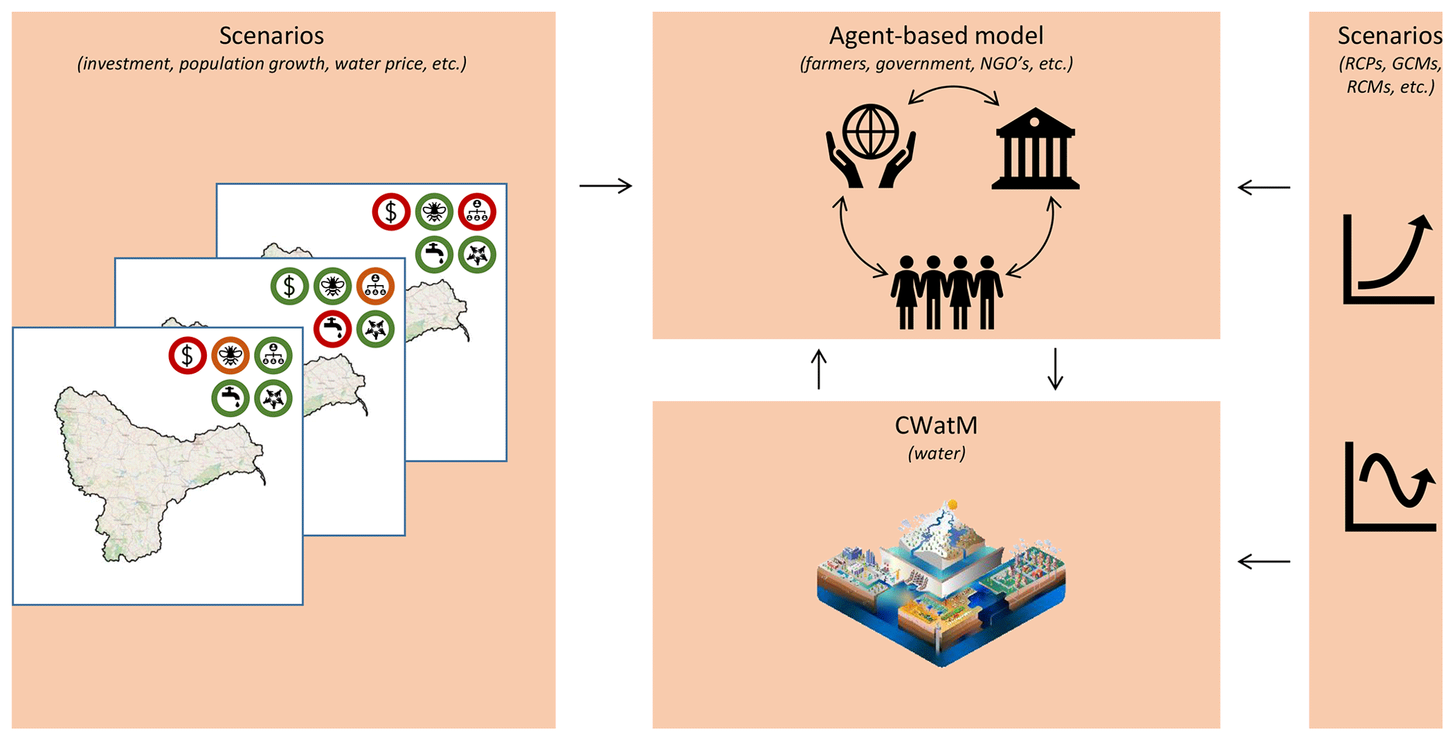
Figure 1 GEB: high-level interaction between CWatM and the agent-based model. © OpenStreetMap contributors 2022. Distributed under the Open Data Commons Open Database License (ODbL) v1.0.

Figure 2 shows further detail on the main model interlinkages between the human and hydrological components. The model consists of two dynamically integrated parts, which run synchronized at a daily time step: a field-scale hydrological model (blue; see Sect. 2.1 for details) and an agent-based model that simulates crop farmers and reservoir managers (orange; see Sect. 2.2 for details).

Figure 2 A schematic overview of GEB.

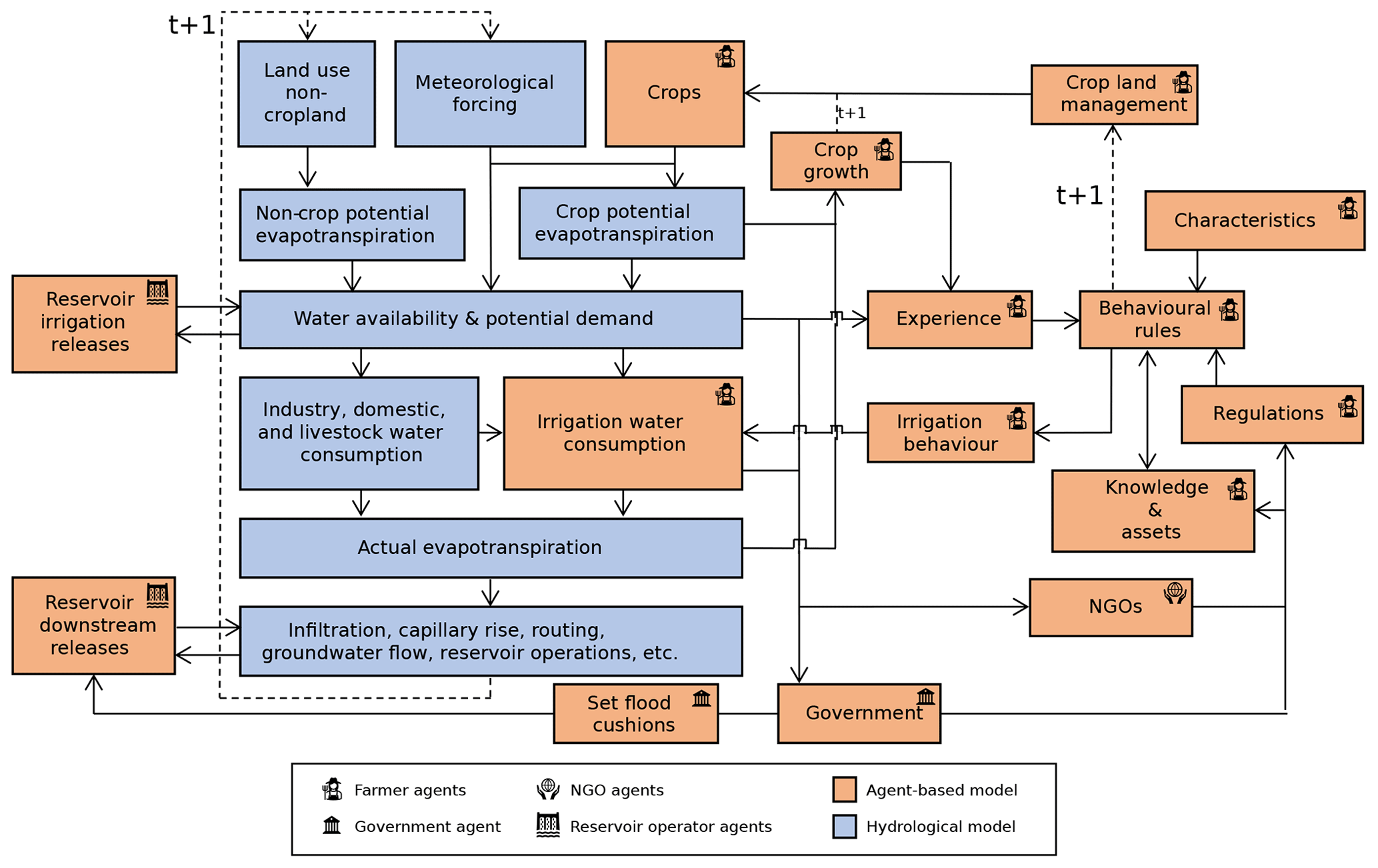
During each time step, the model is forced by a daily set of meteorological data, considering the distribution of land use and crops. Potential evapotranspiration is determined for both cropland and non-cropland, which is followed by the determination of both the water availability and potential demand. Potential irrigation demand for non-paddy irrigation is computed as the difference between current soil moisture content and the soil moisture content at field capacity in the root zone, limited by the infiltration capacity. The potential irrigation demand for paddy-irrigated land is computed as the difference between the current water level in the paddies and the targeted water level. Here, reservoir operators can release water from their reservoir based on considerations such as current demand and water levels. Then, after water consumption by industrial, domestic, and livestock sectors, farmers can abstract irrigation water.

Here, the calculation of water consumption is removed from CWatM and is instead calculated in the agent-based model, addressing irrigation behaviour, selection of crop types, and assets and characteristics of individual agents. These factors are not necessarily static over time, as agents can invest in management options such as irrigation wells, drip irrigation, or change crop types. Moreover, external bodies such as governments and non-governmental organizations (NGOs) can influence the behaviour of farmers and reservoir operators by imposing regulations, providing knowledge to the farmer population or investing in the wider availability of assets (e.g. create an irrigation reservoir). Knowledge can also be obtained from other (neighbouring) agents.

After the application of irrigation water, CWatM simulates infiltration, capillary rise within soils, groundwater recharge, surface routing, and groundwater flow (using MODFLOW; Langevin et al., 2017). Here, CWatM again communicates with the reservoir operator agents to determine the amount of water released downstream. Then, as a new time step is initiated, each farmer can decide to plant or harvest crops based on experience, assets, characteristics, knowledge, and regulations. The land use classes in CWatM are then updated accordingly. Finally, the next time step is initiated, starting with meteorological forcing, as described above.

The model is implemented in Python 3, with all computationally intensive parts written in compiled Python libraries such as NumPy (Harris et al., 2020) and Numba (Lam et al., 2015), and it includes optional GPU vectorization of soil components through CuPy. The model can be run on all major platforms (i.e. Linux, Windows, and Mac). An optional model interface is extended from Mesa (Kazil et al., 2020; Fig. 3). A high-level description of the technical model integration can be found in Appendix A, while further details can be found in the model documentation.

Figure 3 Optional model interface. The model can be run for one more time step, and one can show all model variables on a map. Here, the land use type is shown. The red dots represent farmer agents. Optional line charts can be added to show variables like discharge and mean groundwater level over time. For visualization purposes only, a small subbasin northwest of Pune (Maharashtra) is shown here. Land use map is derived from Jun et al. (2014).

Simulating hydrological processes at the field scale

Most hydrological models implement several different land use types (e.g. Burek et al., 2020; Sutanudjaja et al., 2018; Müller Schmied et al., 2021). In these models, soil processes in all land use types are simulated individually. Runoff and several other hydrological fluxes are then computed by aggregating to the grid cell level while considering the relative size of each land use type in a grid cell. In other words, each land use type within a grid cell is simulated as a HRU (Flügel, 1997; Chaney et al., 2016). Farmers usually occupy cropland land use types such as non-irrigated land, paddy-irrigated land, and non-paddy irrigated land (Burek et al., 2020; Sutanudjaja et al., 2018; Hanasaki et al., 2018; Alcamo et al., 2003). When a single land use type within a grid cell is occupied by multiple farmers, these farmers share a HRU (i.e. hydrological environment) and are thus simulated as a single unit (of multiple farmers).

This introduces an issue for agent-based models that focus on the implementation of heterogeneous decision-making at the field scale. For example, when two farmers share a HRU and farmer no. 1 decides to irrigate while farmer no. 2 does not, the soil moisture in the field of farmer no. 1 should increase relative to the soil moisture in the field of farmer no. 2. However, when both farmers share a HRU, the soil moisture in their field cannot be separately simulated in the model.

The most straightforward solution is to run the model at a higher resolution, such that the smallest field is simulated as a single grid cell while larger fields are simulated as multiple grid cells. However, as small farms of less than 1 ha make up 72 % of global farms (Lowder et al., 2016), this solution requires the use of grid cells that are less than 100 × 100 m, which would use an enormous amount of computational resources, making the approach unfeasible in larger basins.

As a solution, we simulate the field of each farmer as a single HRU and adapt CWatM to be able to work with these HRUs (Fig. 4). In this concept, cropland land use types are further subdivided into dynamically sized HRUs based on the land ownership (or rent) of the agent (e.g. a farmer). These HRUs can be independently operated by agents in the ABM, such as farmers. In this manner, the land management decisions (e.g. crop planting date and irrigation) and soil processes (e.g. percolation, capillary rise, and evaporation) are independently simulated in a HRU for each farmer, thus allowing for simulation of multiple independently operated farms within a single grid cell. These HRUs can also be split, allowing, for example, for farmland expansion into other land use types and the sale of (part of) a farmer's land.

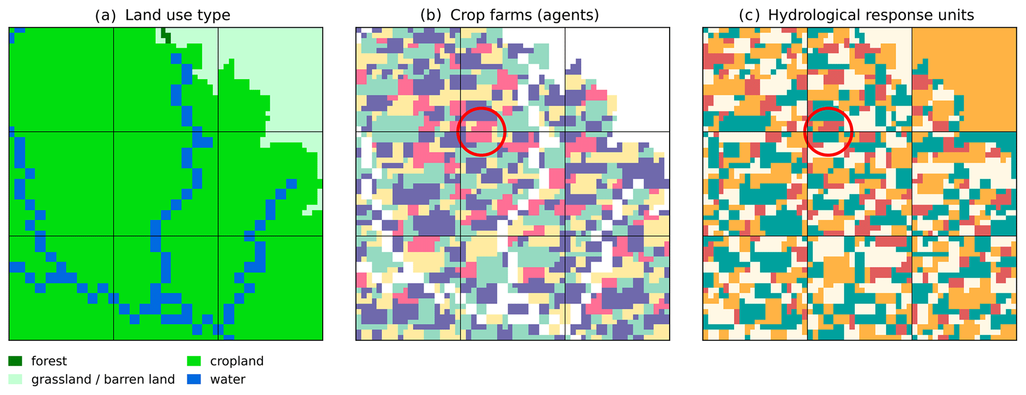
Figure 4 In this figure, 3 × 3 grid cells are shown, delineated by horizontal and vertical black lines (30^′′ resolution). Panel (a) displays various land use types at 20 times higher subgrid resolution, panel (b) shows the crop farms owned by agents, and panel (c) shows the resulting HRUs. Each contiguous area of one colour in panel (b) represents a farm, while each contiguous area of one colour in panel (c) represents a HRU. One exception is non-crop HRUs of the same land use type within a grid cell, which belong to one HRU (e.g. all rivers within a grid cell are 1 HRU). Crop farms owned by one farmer that cross grid cell boundaries are represented by multiple HRUs; see, for example, the crop farm in the centre of the red circle. Land use map is derived from Jun et al. (2014).

Each crop farm that is owned by a farmer is thus an individual HRU. An exception is when a crop farm is spread across multiple grid cells, in which case it is represented by multiple HRUs across those grid cells. However, as these split HRUs are owned by a single farmer, management decisions still affect all HRUs and thus the entire farm. In addition, each land use type that is not operated by crop farmers in a grid cell is a separate HRU, thus operating independently from other land use types, such as water areas, grasslands, and forests.

While most primarily vertical hydrological fluxes (e.g. infiltration, percolation) occur within HRUs, river discharge and groundwater flow are simulated at the grid cell level. To this extent, conversion of fluxes between HRUs and grid cells is required. Figure 5 shows how this works in practice, similar to hydrological models that simulate multiple land use types in a single grid cell, such as CWatM and PCR-GLOBWB (Sutanudjaja et al., 2018). Runoff is first determined per HRU and then aggregated to the grid cell level while considering the relative size of each HRU. Aggregated runoff is then added to discharge, followed by solving the kinematic wave equation at the grid cell level.

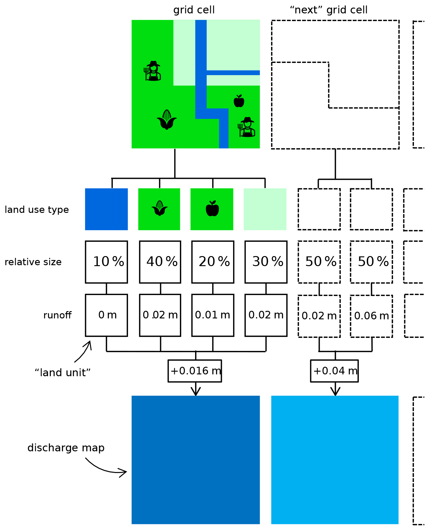
Figure 5 Schematic overview of the implementation of farm-level HRUs. Here, a grid cell consists of four HRUs: one water-covered area, two crop farms, and one grass-covered area (see coloured land use types). Runoff is determined per HRU and then aggregated by considering the relative size of the HRUs to compute runoff for the entire grid cell.

For the implementation in the Krishna basin, we selected the region basin for the study using the globally available MERIT Hydro elevation map (Yamazaki et al., 2019), which was upscaled to 30^′′ by using the iterative hydrography upscaling method (Eilander et al., 2021) and by subsequently selecting all upstream cells of the Krishna River outlet. Other routing maps, such as river slope and width, were obtained similarly (Eilander et al., 2020). Reservoir and lake footprints were obtained from the HydroLAKES dataset (Messager et al., 2016). If available, flood cushions and reservoir volumes were obtained from the Andhra Pradesh WRIMS (https://apwrims.ap.gov.in/, last access: 7 September 2021) database. If not available, flood cushions were assumed to be zero, while reservoir volumes were taken from the original HydroLAKES data. Reservoir command areas were obtained from the India Water Resources Information System (India-WRIS, https://indiawris.gov.in/wris/, last access: 7 September 2021) and manually linked to the previously obtained reservoir using satellite imagery. Reservoir operator agents are assumed to release a maximum fraction of the current reservoir volume for irrigation, limited by the irrigation demand in the command area. Land use was obtained at 30 m resolution from GlobeLand30, downscaled to 1.5^′′ and mapped to CWatM land use types. Pixels that were classified as “waterbody” in GlobeLand30 and all cells with at least 100 km² upstream area were classified as “water covered area” in CWatM. All other input data were obtained from CWatM input maps at 5^′ resolution and downscaled to 30^′′ for CWatM input. The groundwater MODFLOW model is defined by an orthogonal grid at a 1000 m resolution. Only one homogeneous unconfined aquifer layer is considered. One pumping well is set up in each MODFLOW cell to satisfy the water demand from farmers and other sectors.

Water demand and consumption for industrial, domestic, and livestock sectors are estimated using the approach developed by Wada et al. (2011) and are then downscaled to the size of the HRUs by distributing the demands over cells with relevant land uses: grassland for livestock demands and sealed area for industrial and domestic demands. The model was forced with GSWP3 (Dirmeyer et al., 2006), provided as part of ISIMIP3a (Warszawski et al., 2014).

3 Model application

Here, we show the application of the model in the heavily managed Krishna basin in India, simulating the behaviour of more than 12 million farmers and the water system. With a size of roughly 8 % of India's land area, the Krishna basin in India (Fig. 6) is a complex socio-ecological system experiencing several sustainability and equity challenges particularly related to water resources management. For example, some farmers have access to large amounts of irrigation water, leading to dropping groundwater tables in the entire region, affecting small farmers without a (deep) well disproportionately. The basin is important for agricultural production while being exposed to floods, droughts, and dropping groundwater tables (Surinaidu et al., 2013). A large number of reservoirs with a total volume of approximately 42 ×10⁹ m³ (∼ 20 % of annual rainfall) were built primarily for irrigation purposes. Farmers in a reservoir command area can access the reservoir water that is distributed through a system of canals. In addition, following the Indian Agriculture Census (http://agcensus.dacnet.nic.in/, last access: 7 October 2022), approximately 8 % of farmers have access to groundwater through a well, depending on the farm size and location. The mean farm size is ∼ 1.5 ha. Soils largely consist of clay, silt, and sand. The predominant rock type found in the Western Ghats is basalt.

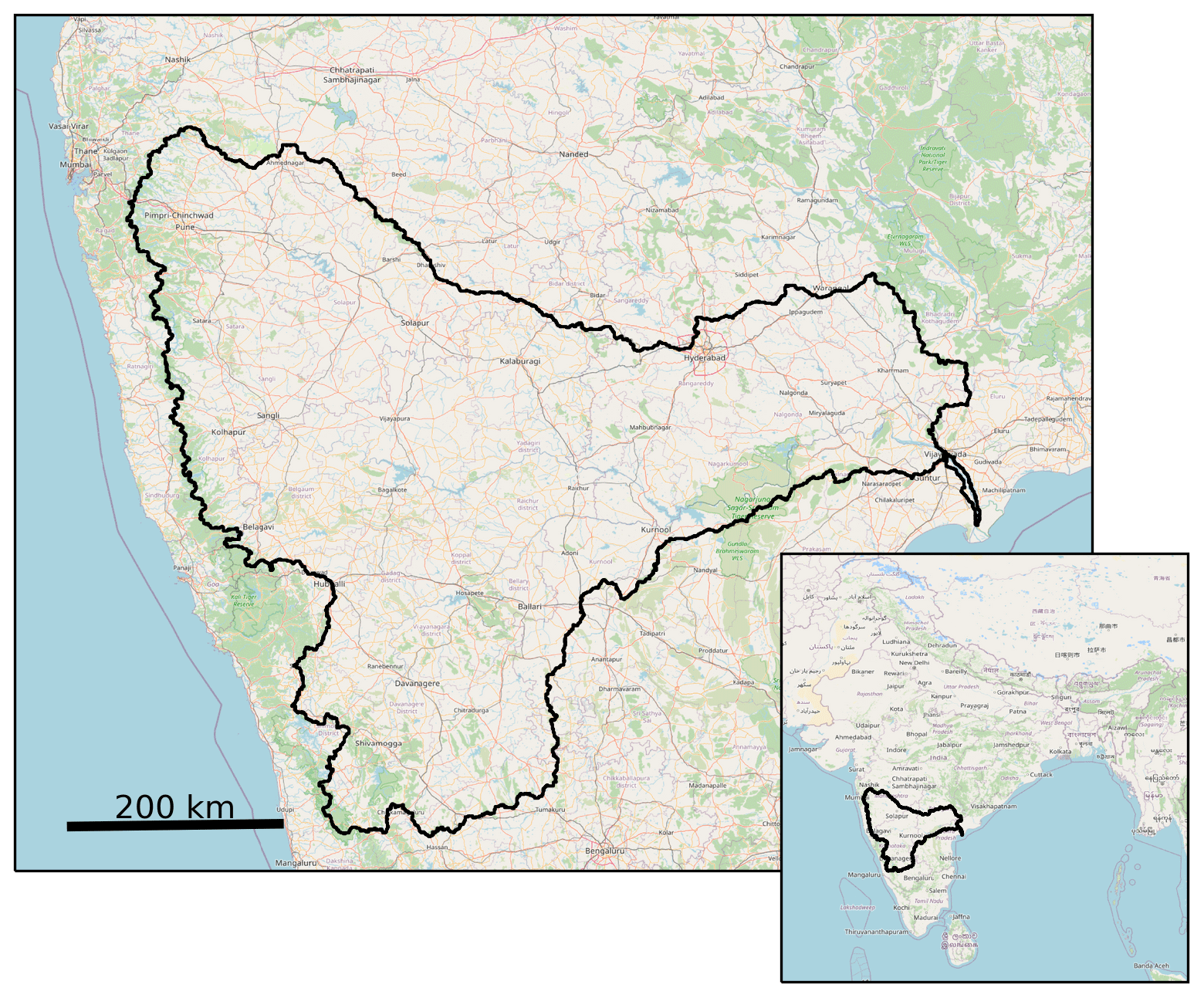
Figure 6 Outline of the Krishna basin in India. © OpenStreetMap contributors 2022. Distributed under the Open Data Commons Open Database License (ODbL) v1.0.

3.1 Agents

The ABM has farmer (Sect. 3.1.1) and reservoir operator agents (Sect. 3.1.2), which can make autonomous decisions affecting the hydrological system as well as each other. Farmers and reservoir operators directly interact with CWatM.

Figure 7 Schematic overview of the iterative proportional fitting (IPF) algorithm.

3.1.1 Farmers

Farmer initialization

First, an initial agent population needs to be generated with heterogeneous characteristics similar to the real population living in the basin. As with most agent-based models, and in particular large-scale models, we do not have specific information for every person. Therefore, we generate a synthetic population of farmers which has statistically similar properties to the real population (income, irrigation type, household size, etc). These statistics are based on available survey data combined with regional marginal statistics using the iterative proportional fitting algorithm (IPF; Fig. 7). For the implementation in the Krishna basin, the IPF algorithm reweights survey data from the India Human Development Survey (IHDS; Desai et al., 2005) such that the overall distribution of the adjusted survey data fits the marginal distributions of farm sizes and crop types at subdistrict-level based on the Indian Agriculture Census (https://agcensus.dacnet.nic.in/, last access: 7 October 2022). Here, we consider all crops that are grown by at least 2 % of the farmer population. Because farmers with multiple crop types throughout the year are counted multiple times in the census, an adjusted version of IPF is used (Appendix B). In this manner, a heterogeneous population of 12.2 million farmers is generated with the following characteristics: household size; crop type in kharif, rabi, and summer seasons; irrigation type; daily non-farm income; and daily consumption per capita.

Next, the farmer population is randomly distributed within their subdistrict on farmland as specified in GlobeLand30 (Jun et al., 2014), at a 1.5^′′ resolution (i.e. 20 times higher resolution than the CWatM grid; < 50 m at the Equator). The smallest field size is thus approximately 0.25 ha.

Cropping

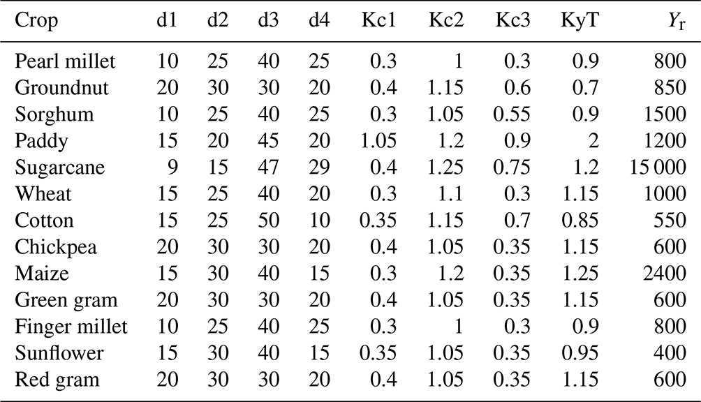
The generated farmer agents grow the following crops: pearl millet, groundnut, sorghum, paddy rice, sugar cane, wheat, cotton, chickpea, maize, green gram, finger millet, sunflower and red gram. Each crop has four growth stages ($d_{\mathrm{1}},\mathrm{\dots },d_{\mathrm{4}}$). The crop factor (Kc) is then calculated based on the following equation (Fischer et al., 2021):

$$\begin{array}{}\text{(1)}& \begin{array}{rl}& {\mathrm{Kc}}_t=\\ & \left\{\begin{array}{ll}\mathrm{Kc}\mathrm{1},& t<d_{\mathrm{1}}\\ \mathrm{Kc}\mathrm{1}+\left(t-d\mathrm{1}\right)\times \frac{\mathrm{Kc}\mathrm{2}-\mathrm{Kc}\mathrm{1}}{d\mathrm{2}},& d_{\mathrm{1}}\le t<d_{\mathrm{2}}\\ \mathrm{Kc}\mathrm{2},& d_{\mathrm{2}}\le t<d_{\mathrm{3}}\\ \mathrm{Kc}\mathrm{2}+(t-\left(d\mathrm{1}+d\mathrm{2}+d\mathrm{3}\right))\times \frac{\mathrm{Kc}\mathrm{3}-\mathrm{Kc}\mathrm{2}}{d\mathrm{4}},& \text{otherwise};\end{array}\right.\end{array}\end{array}$$

where t is the number of days after the crop has been planted, and d₁ to d₄ represent the length of each crop stage. At the harvest stage, actual yield (Y_a) is calculated using a reference yield (Y_r; Siebert and Döll, 2010), the water-stress reduction factor (KyT), and the ratio of actual evapotranspiration (AET) to potential evapotranspiration (PET) over the entire growing period (Fischer et al., 2021).

$$\begin{array}{}\text{(2)}& Y_{\mathrm{a}}=Y_{\mathrm{r}}\times \left(\mathrm{1}-\mathrm{KyT}\times \left(\mathrm{1}-{\displaystyle \frac{{\sum }_{t=\mathrm{0}}^{t=h}{\mathrm{AET}}_t}{{\sum }_{t=\mathrm{0}}^{t=h}{\mathrm{PET}}_t}}\right)\right)\end{array}$$

All crop-specific factors used in Eqs. (1) and (2) can be found in Table C1.

Farmer income and expenses

After harvesting, it is assumed that farmers sell their crops for the state-wise market price for that month. Historic monthly market prices are obtained from Agmarknet (https://agmarknet.gov.in/, last access: 27 July 2022) for all crops except sugar cane. For sugar cane, which is brought directly to sugar cane mills, it is assumed that farmers receive the yearly indexed fair and remunerative price (FRP). These prices are fixed by the government. Yearly cultivation costs (e.g. purchasing seeds, manure, labour cost, annual depreciation) per hectare per crop type are obtained from the Ministry of Agriculture and Farmers Welfare (https://eands.dacnet.nic.in/Cost_of_Cultivation.htm, last access: 15 July 2022). Additional farmer income is obtained (e.g. from non-farming work) from the IHDS survey data. Similarly, living expenses are calculated from the daily consumption per capita in each household and household size, both available from the IHDS survey. Finally, disposable income is calculated by subtracting income and expenses.

Irrigation

During the model run, when a farmer F has irrigation equipment and is cultivating a crop, they irrigate the HRUs they own (Fig. 8).

Figure 8 Farmer irrigation procedure; see also Eqs. (3)–(6).

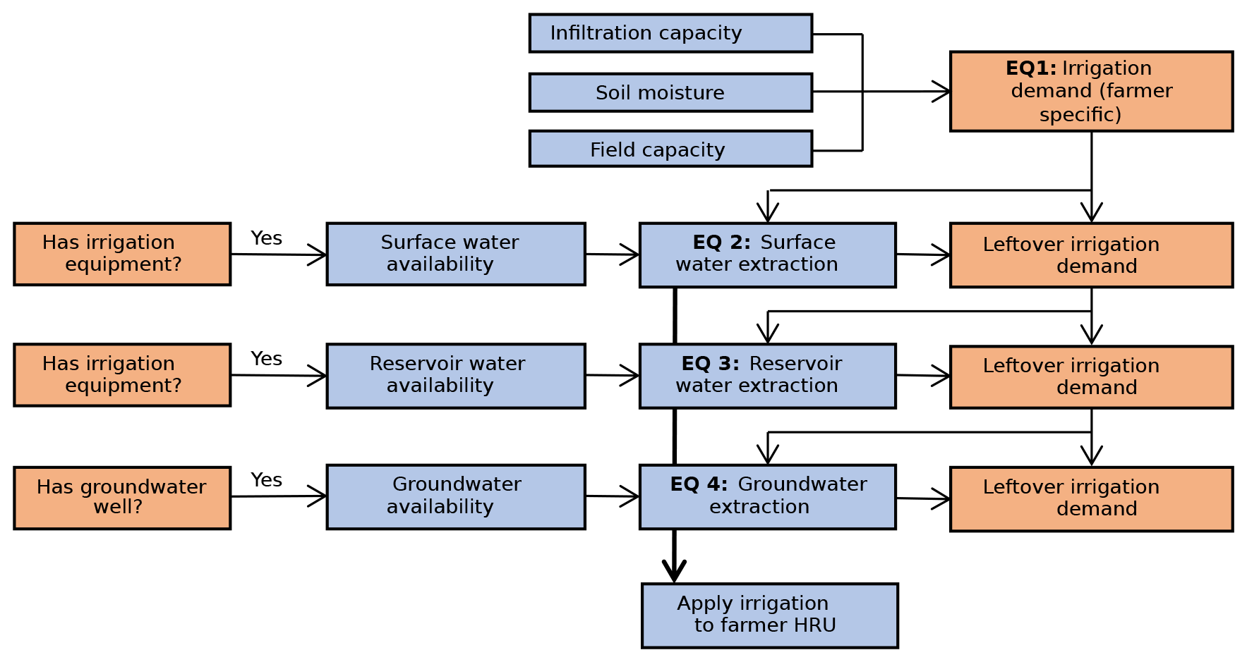
Agents are allowed to abstract water first on a first-come, first-served principle, starting with upstream agents as determined by their elevation. As agents have no incentive to consider environmental flow conditions, these are not enforced. Farmer irrigation demand (dem) is determined by the difference between field capacity (FC) and soil moisture (SM) and is limited by infiltration capacity (IC). If farmers have access to the right equipment for surface (F_sw), reservoir (F_res), and groundwater irrigation (F_gw), irrigation demand (dem) is then satisfied (Eq. 3), first from surface water (Eq. 4), then from reservoirs (Eq. 5), and finally from groundwater (Eq. 6). All sources are limited to current water availability from the streamflow (avail_sw) in grid cell G, reservoirs (avail_res) that supply the command area of grid cell G, and groundwater in grid cell G. In addition, farmers only have access to water resources if they have the relevant irrigation equipment.

$$\begin{array}{}\text{(3)}& {\displaystyle }{\mathrm{dem}}_{\mathrm{HRU}}=min({\mathrm{FC}}_{\mathrm{HRU}}-{\mathrm{SM}}_{\mathrm{HRU}},{\mathrm{IC}}_{\mathrm{HRU}});\text{(4)}& {\displaystyle }\begin{array}{rl}& {\mathrm{irr}}_{\mathrm{HRU},\mathrm{sw}}=\\ & \left\{\begin{array}{ll}\mathrm{0},& F_{\mathrm{sw}}=\mathrm{False}\\ min\left({\mathrm{dem}}_{\mathrm{HRU}},{\mathrm{avail}}_{\mathrm{sw},G}\right),& F_{\mathrm{sw}}=\mathrm{True};\end{array}\right.\end{array}\text{(5)}& {\displaystyle }\begin{array}{rl}& {\mathrm{irr}}_{\mathrm{HRU},\mathrm{res}}=\\ & \left\{\begin{array}{ll}\mathrm{0},& F_{\mathrm{res}}=\mathrm{False}\\ min\left({\mathrm{dem}}_{\mathrm{HRU}}-{\mathrm{irr}}_{\mathrm{HRU},\mathrm{sw}},{\mathrm{avail}}_{\mathrm{res}}\right),& F_{\mathrm{res}}=\mathrm{True};\end{array}\right.\end{array}\text{(6)}& {\displaystyle }\begin{array}{rl}& {\mathrm{irr}}_{\mathrm{HRU},\mathrm{gw}}=\\ & \left\{\begin{array}{ll}\mathrm{0},& F_{\mathrm{gw}}=\mathrm{False}\\ min\left({\mathrm{dem}}_{\mathrm{HRU}}-{\mathrm{irr}}_{\mathrm{HRU},\mathrm{sw}}-{\mathrm{irr}}_{\mathrm{HRU},\mathrm{res}},{\mathrm{avail}}_{\mathrm{gw},G}\right),& F_{\mathrm{gw}}=\mathrm{True};\end{array}\right.\end{array}\end{array}$$

When a farmer decides to irrigate, the water is subtracted from the relevant sources in CWatM and then applied to the land in the relevant HRU.

The planting and harvesting dates are dependent on crop type and growing pattern. Once the farmer decides to harvest their crop, the respective HRU is set to “barren land” in CWatM. Then, as the farmer decides to plant a new crop, the land use type is changed accordingly in CWatM (e.g. to “irrigated”).

Investing in irrigation wells

On the first day of each year, farmers can choose to invest in an irrigation well to improve their ability to irrigate their land. Here, we use the expected utility theory (e.g. Schrieks et al., 2021) to assess whether farmers make such an investment. Due to the strong social network effects (e.g. Tripathi and Mishra, 2017), we consider that farmers assess the potential benefit of installing an irrigation well based on the profit of neighbouring farmers with an identical cropping pattern but with an existing irrigation well. More specifically, we first calculate the farmer “profit ratio” (r_own) [0–1], defined by the ratio of actual profit to potential profit given abundant water (i.e. actual evapotranspiration is equal to potential evapotranspiration). Each farmer without an irrigation well compares their profit ratio to the profit ratio of 10 nearby farmers with an identical cropping pattern but no irrigation well (r_neighbours). The benefit of installing an irrigation well is then calculated by multiplying the difference by the current crop price (P) and reference yield (Y_r). Similarly, costs for well installation are calculated by considering the costs of a loan for that amount (Y_r), considering loan duration in years (n), the current interest rate (i), and yearly upkeep cost (U). Finally, incremental profit (Δπ) is determined by subtracting costs and benefits. If Δπ is positive, the farmer invests in the irrigation well.

$$\mathrm{\Delta }\mathit{\pi }=P\times Y_{\mathrm{r}}\times \left(r_{\mathrm{neighbours}}-r_{\mathrm{own}}\right)-\left({\displaystyle \frac{C}{n}}+C\times i+U\right)$$

The interest rate is set to the lending interest rate in India for that year (https://data.worldbank.org/indicator/FR.INR.LEND?locations=IN, last access: 3 January 2023); tube well installation and maintenance costs for the year 2008 are set at INR 146 000 and 3000 per hectare, respectively (Sharma et al., 2008), and corrected for inflation for other years. Loan duration is set to 10 years, following offerings of several major agricultural banks in India. Finally, it is determined whether current disposable income is sufficient to pay for the loan. All installed wells are assumed to be 30 m deep.

3.1.2 Reservoir operators

The reservoir operator agents communicate with farmer agents in their reservoir command area on a daily basis and release the requested water for irrigation purposed, maximized by a maximum percentage of the current reservoir water volume. As upstream farmers get to abstract water first, this can lead to limited access to reservoir water for farmers at the tail end of command areas. The amount of water released for other purposes (e.g. maintaining outflow, reducing water level) depends on the rating curve of the reservoir and relevant flood cushions (Burek et al., 2020).

3.2 Calibration and validation

The model is calibrated based on daily river discharge from the India Water Resources Information System (WRIS) for the Wadenepally station in the Krishna River, nearby the river outlet, roughly 60 km upstream of Vijayawada. Calibration is performed based on several hydrological parameters (Burek et al., 2020), as well as the maximum amount of water released from a reservoir for irrigation purposes on a given day, the normal reservoir outflow, and the irrigation return fraction. Using the NSGA-II genetic algorithm (Deb et al., 2002), as implemented in DEAP (Fortin et al., 2012), the calibration procedure optimizes the modified version of the Kling–Gupta efficiency score (KGE; Eq. 5; Kling et al., 2012):

$$\begin{array}{}\text{(7)}& {\mathrm{KGE}}^{\prime }=\mathrm{1}-\sqrt{{\left(r-\mathrm{1}\right)}^{\mathrm{2}}+{\left(\mathit{\beta }-\mathrm{1}\right)}^{\mathrm{2}}+{\left(\mathit{\gamma }-\mathrm{1}\right)}^{\mathrm{2}}},\end{array}$$

where r is the correlation coefficient between monthly simulated and observed discharge, $\mathit{\beta }=\frac{{\mathit{\mu }}_{\mathrm{s}}}{{\mathit{\mu }}_{\mathrm{o}}}$ is the bias ratio, and $\mathit{\gamma }=\frac{{\mathrm{CV}}_{\mathrm{s}}}{{\mathrm{CV}}_{\mathrm{o}}}=\frac{{\mathit{\sigma }}_{\mathrm{s}}/{\mathit{\mu }}_{\mathrm{s}}}{{\mathit{\sigma }}_{\mathrm{o}}/{\mathit{\mu }}_{\mathrm{o}}}$ is the variability ratio; r, β, and γ are all optimal at 1.

The period 2004–2006 is used as a spin-up period, the period 2006–2012 is used for calibration, and the period 2012–2019 is used for validation. The genetic calibration algorithm first generates 60 parameter sets within a predefined range of plausible options (i.e. “the population”), and the model is subsequently run for each parameter set (i.e. “individual”). The 10 most optimal parameter sets are then combined (i.e. “mated”) with a probability of 0.7 or altered (i.e. “mutated”) with a probability of 0.3 to create 12 new parameter sets for which the model is also run. This procedure is repeated for 10 iterations (i.e. “generations”), and the most optimal parameter set is selected. This set is then re-run until the year 2019, and the KGE score is calculated for 2013–2019 for validation.

4 Results and discussion

Figure 9 shows observed versus simulated discharge (in m³ s⁻¹) for the calibration model. The KGE during the calibration period is 0.810, while the KGE during the test period is 0.834 (1 is optimal), showing a good calibration performance for the model during both periods.

Figure 9 Observed versus simulated discharge for the calibrated model.

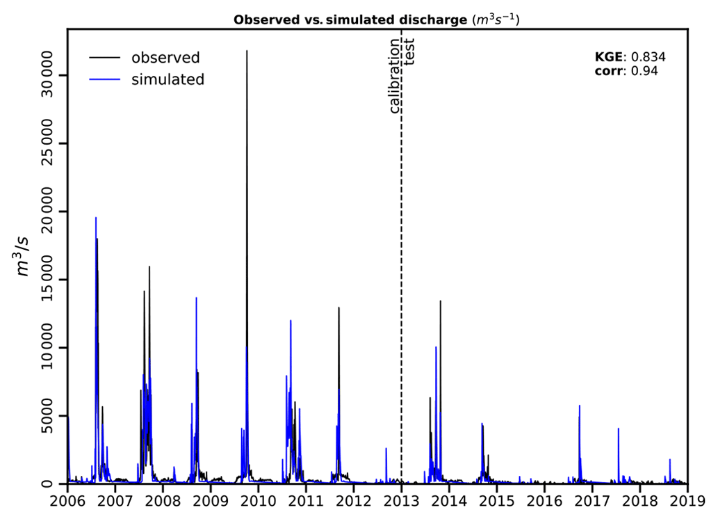
Figure 10 shows irrigation from channels, reservoirs, and groundwater for all agents for the Krishna basin. The insets show the detailed heterogeneous quantities at the field scale for a small portion of the basin. Yet, on the larger scale, it is clearly visible that farmers along rivers and within reservoir command areas have better access to water for irrigation. Differences in irrigation quantities from various sources are explained due to the location of farmers (and hence access to water from various irrigation sources), crop types, irrigation equipment, etc. For example, farmers without an irrigation well cannot access the groundwater and thus can irrigate less, while farmers with sugar cane are expected to irrigate more than other farmers.

Figure 10 Average daily irrigation from channels, reservoirs, and groundwater.

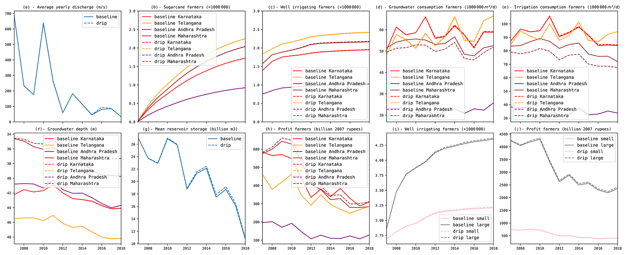
Figure 11 Yearly simulation results for baseline scenario and scenario with investment in drip irrigation.

In Fig. 11, we show how several variables change over time for specific scenarios, with the aim of showing how the model behaves. In the baseline scenario, farmers that have access to a reliable irrigation well have a 20 % probability of switching to sugar cane, a crop that generally ensures a higher income but also uses a lot of water. Here, we define a reliable irrigation well as a well that has not fallen dry in the last 3 years. The resulting mean annual discharge is shown in panel (a), while the number of farmers with sugar cane in each state gradually increases over time, as shown in panel (b). Similarly, the number of wells increases over time (panel c), due to investment in irrigation wells (see Sect. “Irrigation”). Panels (d) and (e) show the amount of irrigation from the groundwater and total irrigation from all sources. Because of the increasing number of irrigation wells, as well as other factors, groundwater abstraction generally outpaces recharge, and thus the groundwater table decreases in all four states. The mean reservoir storage also decreases over time. However, profit, when adjusted for inflation, decreases over time (panel h) as less water is available for farmers and prices increase for crops at the market (e.g. 83 % increase in average price at the crop market for the analysed crops for Maharashtra, while general prices are 122 % higher). Finally, panels (i) and (j) show how the number of irrigation wells and profit change for farmers practicing small- and larger-scale farming. Here, smallholder farmers are the 50 % of farmers with the smallest fields, while farmers practicing large-scale farming are those with the 50 % largest fields. It is clear that smallholder farmers have less irrigation wells (panel i) at the beginning of the run but also can invest less in irrigation wells due to their limited income compared with farmers practicing large-scale farming (Sect. “Irrigation”). This is also reflected in the profits. The relative increase in profits is approximately 2 % higher for large farms over the entire simulation timeline.

In another hypothetical scenario called drip (see Fig. 11), the state of Maharashtra, one of the upstream states, provides subsidies to farmers, making 20 % of farmers switch to drip irrigation each year, corresponding with a 90 % irrigation efficiency (Brouwer and Heibloem, 1986). Here, yearly discharge (at the basin outlet) increases slightly in some years (here: 2016 only), likely because most additional water is used downstream due to the large number of reservoirs and reservoir command areas downstream of Maharashtra. The mean combined reservoir storage is slightly higher in this scenario (panel g). Interestingly, the number of installed irrigation wells (panel c) also goes up in Maharashtra, Karnataka, and Telangana, likely because fewer wells fall dry. This means that the benefit of having an irrigation well increases (mostly Maharashtra), and the means to invest in an irrigation well also increase due to higher water availability and thus higher yield (mostly Maharashtra and Karnataka). In Karnataka and Telangana, this even leads to a slight decrease in the water table.

While some adaptation options are considered here, additional adaptation options could be considered at a later stage such as crop switching and rainwater harvesting (Tamburino et al., 2020). Moreover, other factors can be included, such as threat appraisal (e.g. perception of drought risk), the coping appraisal of individual farmers (e.g. knowledge, information, and financial resources; Wens et al., 2020; Schrieks et al., 2021; Streefkerk et al., 2023), an extension of farmer networks (Wens et al., 2020), and collective adaptation behaviour by farmer cooperatives. In addition, model parameterization could benefit from the automatic delineation of smallholder fields using machine learning (Waldner and Diakogiannis, 2020) and the recognition of crop types at the field scale (Gumma et al., 2020) when such datasets become freely available in the future.

5 Conclusions

Here, we present a coupled agent-based hydrological model which for the first time allows for simulation of millions of individual households and their bidirectional interactions with the hydrological system while assessing large-scale hydrological processes. By combining survey data and aggregate statistics at the subdistrict level, the model uses a statistically representative population, considering the heterogeneity of the population and the spatial variability. The open-source model is developed in Python, simulating more than 12 million farmers on an computer with 16 GB of RAM. By adopting a fully distributed hydrological model with dynamically sized field-scale hydrological response units (HRUs), the model can effectively represent subsistence farmers, ensuring that they can individually interact with the hydrological model while keeping computational demands reasonable.

Using the model, we quantitatively show how farmer behaviour and the hydrological system are intricately woven across both small and large scales. Changes in behaviour or investment in irrigation measures affect hydrology and other farmers locally, but they also affect river discharge and other farmers further downstream. Effects are visible both in hydrological variables as well as farmer behaviour and profit. Using a scenario where drip irrigation is promoted in an upstream state, we show how the effect of policies can be assessed on local and large-scale processes across both the hydrological and human domains. This provides opportunities to study large- and small-scale socio-hydrological processes simultaneously in large river basins worldwide. Moreover, capturing the full heterogeneity of the farmer populations allows for investigation of equity issues, particularly related to distributional justice.

The agent-based model can be separately coupled to other hydrological models, assuming the hydrological model facilitates simulation of field-scale hydrological processes. Alternatively, at the price of losing the ability to fully capture heterogeneity of human processes, the ABM can be adapted to simulate aggregated agents within a grid cell, facilitating coupling to other hydrological models that do not support field-scale hydrological simulation. Similarly, the adapted version of CWatM, which now simulates field-scale hydrological processes, can be coupled to other ABMs.

Future studies could include additional adaptation measures to make the model more realistic and further investigate how policies and infrastructural projects, such as through reservoir construction and management, water/electricity pricing (Parween et al., 2021), water rights (Nouri et al., 2019a), and enforcing specific crop types (Wallach, 1984) can affect the human–natural system. As humans play a key role in the environment, the human component of GEB can also be central in coupling further models, e.g. to economic models or land use change models (Dou et al., 2020), allowing us to investigate the land–water–food use nexus. In addition, coupling GEB to a hydrodynamic model such as DIM (Farrag et al., 2021) would allow us to investigate the interactions between human behaviour and flood and drought risk (Ward et al., 2020). Finally, the integration of future scenarios such as climate change, population growth, and exogenous land use can be used to project how the coupled human–natural system changes in the future.

Computational requirements

The model for the entire Krishna basin can be run on a computer with 16 GB of RAM. Model run time was ∼ 10 s per daily time step (i.e. ∼ 1 h for 1 year) using a single core on an AMD EPYC 7302 while requiring no more than 7 GB of RAM and an 8 GB RTX1070 GPU. Without GPU, the run time was ∼ 30 s per time step while requiring 12 GB of RAM. Model run time and requirements scale near-linearly with basin size, assuming identical farm sizes. Larger farm sizes reduce the requirements, while smaller farms increase the requirements. In the implementation in the Krishna basin as shown here, the average farm size is 1.6 ha.

Appendix A

This section discusses the coupling between the ABM and hydrological model, serving as both an explanation to how the coupling has been performed in GEB and, if required, allowing the reader to couple their hydrological model to the ABM or the ABM to their hydrological model. The ABM can be found in the GEB repository (https://github.com/jensdebruijn/GEB, last access: 14 February 2023), while the adapted version of CWatM (see Sect. 2.1) can be found in the ABCWatM repository (https://github.com/jensdebruijn/ABCWatM, last access: 14 February 2023). Because both models are written in Python, the coupling is performed by creating a Python class, which subclasses both models while synchronizing their time steps. By subclassing both models, both models can access variables from the other model, and functions can be adapted, allowing the models to communicate during each time step. The model class first loads the configuration file (default: “GEB.yml”) which contains configuration parameters for both models, such as the start and end dates of the simulation. Then, the shared data class (“self.data”) is loaded, which contains all data that are shared between the models. The data class loads the study area and automatically creates the grid and HRUs using the given land use and farm map (see Sect. 2). This class also contains convenience functions to convert data between the grid and HRUs (e.g. adding up runoff for individual HRUs to the grid level). An example is given in Fig. A1.

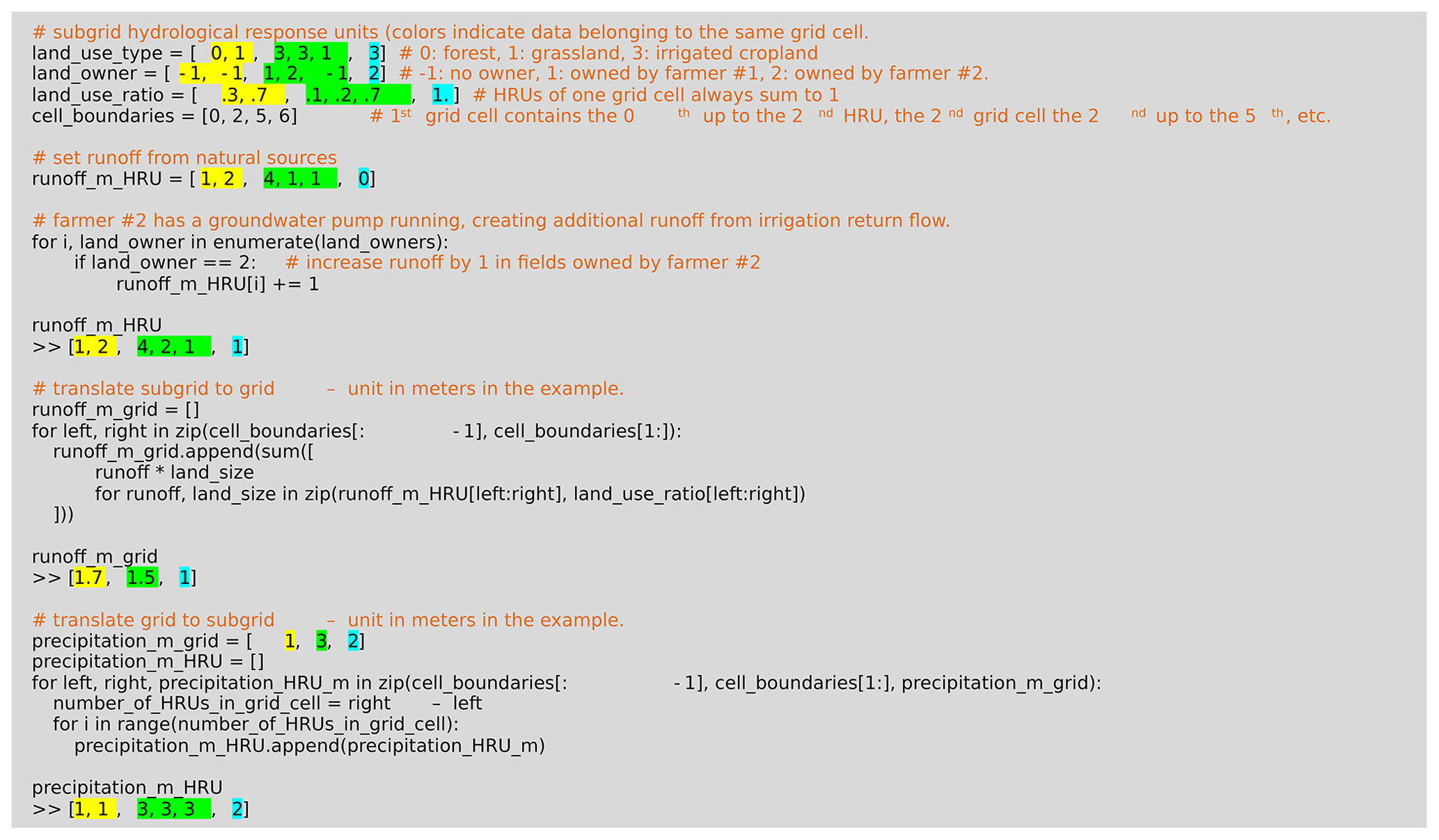
Figure A1 A simplified code example of the conversion between hydrological response units (HRUs) and the grid.

Then, the agent-based model is initialized with agent attributes (see Sect. 2). For farmers, this consists of a raster map that indicates the area that is managed by a specific farmer, the locations of the farms (e.g. the centre point of the each farmers field), and other attributes, such as crop type, cropping schedule, and irrigation status. Subsequently, CWatM is initialized as per Burek et al. (2020) while loading initial land use and crop parameters from the ABM.

After initialization, the (daily) time steps of the ABM and the hydrological model are synchronized. First, farmers make decisions based on the current conditions (e.g. planting, harvesting, investing), followed by the hydrological model which simulates hydrological processes, including water demand. For all sectors excluding crop farming, water demand is simulated as exogenous input. However, for crop water, demand and consumption are determined by the ABM. To this extent, CWatM calls a function (i.e. “abstract_water()”) in the ABM that determines these demand and consumption rates using current soil moisture content; available water from surface, reservoir, and groundwater; and farmer characteristics such as irrigation equipment, crop type, and location.

Appendix B

The iterative proportional fitting (IPF) algorithm reweights the sample weights from survey data in such a way that the aggregate statistics of the reweighted survey data match those of the marginal distributions. To do so, it is required that before initialization of the algorithm the sum of initial weights matches the marginal distribution (e.g. when there are 500 women and 500 men in the marginal distribution, the sum of the initial weights must be 1000). However, here one of the statistics we use is crop type. In the synthetic population, we require crop type per agricultural season (i.e. kharif, rabi, and summer). In the IHDS, this is specified accordingly but not in the Indian Agricultural Census. Here, only the total area per crop is specified. If a farmer uses different crops per season, the area is counted twice. In the IPF procedure, it is thus required to combine the crops from the survey data and then fit the combined crops to the census data, which means that the total number of crops is higher than the total number of farmers (assuming at least one farmer is multi-cropping in the region. To this extent, we adapt the IPF procedure in three ways to ensure correct fitting:

1. Entries in the survey data are reweighted based on the mean target for all crops within that entry. For example, to obtain the correct values at the tehsil level, sugar cane needs to be multiplied by 2.0, while rice needs to be multiplied by 0.8. In that case, the weight attributed to a farmer who grows both sugar cane and rice is multiplied by 1.6 (i.e. 2.0 × 0.8), while the weight attributed to another farmer who only grows rice is multiplied by 0.8.

2. A learning rate is introduced, meaning that the reweighting is not done at once, but changes are gradual following the learning rate. Here we set the learning rate to 0.1.

3. After reweighting all farmers, the entire survey is reweighted to ensure that the total number of farmers is still identical to the initial number of farmers.

Appendix C

Table C1 displays the crop growth stages, crop factors, and water-stress reduction factors for all crops included in the implementation in the Krishna basin.

Table C1 Crop growth stages, crop factors, and water-stress reduction factors.