the Creative Commons Attribution 4.0 License.
the Creative Commons Attribution 4.0 License.
 | 17 Apr 2023
Evaluation of bias correction methods for a multivariate drought index: case study of the Upper Jhelum Basin
Ana Casanueva
Muhammad Usman Liaqat
Giovanna Grossi
Bias correction (BC) is often a necessity to improve the applicability of global and regional climate model (GCM and RCM, respectively) outputs to impact assessment studies, which usually depend on multiple potentially dependent variables. To date, various BC methods have been developed which adjust climate variables separately (univariate BC) or jointly (multivariate BC) prior to their application in impact studies (i.e., the component-wise approach). Another possible approach is to first calculate the multivariate hazard index from the original, biased simulations and bias-correct the impact model output or index itself using univariate methods (direct approach). This has the advantage of circumventing the difficulties associated with correcting the inter-variable dependence of climate variables which is not considered by univariate BC methods.
Using a multivariate drought index (i.e., standardized precipitation evapotranspiration index – SPEI) as an example, the present study compares different state-of-the-art BC methods (univariate and multivariate) and BC approaches (direct and component-wise) applied to climate model simulations stemming from different experiments at different spatial resolutions (namely Coordinated Regional Climate Downscaling Experiment (CORDEX), CORDEX Coordinated Output for Regional Evaluations (CORDEX-CORE), and 6th Coupled Intercomparison Project (CMIP6)). The BC methods are calibrated and evaluated over the same historical period (1986–2005). The proposed framework is demonstrated as a case study over a transboundary watershed, i.e., the Upper Jhelum Basin (UJB) in the Western Himalayas.
Results show that (1) there is some added value of multivariate BC methods over the univariate methods in adjusting the inter-variable relationship; however, comparable performance is found for SPEI indices. (2) The best-performing BC methods exhibit a comparable performance under both approaches with a slightly better performance for the direct approach. (3) The added value of the high-resolution experiments (CORDEX-CORE) compared to their coarser-resolution counterparts (CORDEX) is not apparent in this study.
- Article
(11102 KB) - Full-text XML
-
Supplement
(3454 KB) - BibTeX
- EndNote


Weather and climate-related extreme events (floods, droughts, heat waves, storms, etc.) that arise from complex interactions of various physical processes across multiple scales in space and time are projected to be amplified under global warming conditions and thus are expected to create huge societal and ecological impacts (Kopp et al., 2017; Zscheischler et al., 2018; Raymond et al., 2020; Zscheischler et al., 2020). Such projected climate assessments are usually undertaken using impact models or hazard indices under different global warming scenarios. Those hazard indices and impact models have been developed according to the needs of different sectors, and they are usually based on one or more essential climate variables (ECVs). For instance, maximum consecutive 5 d precipitation and the number of days with minimum temperature above 20 ∘C rely on one ECV only, i.e., precipitation and temperature, respectively, while some require more complex calculations (e.g., the river flow index using runoff based on the results of hydrological model simulations).
Several studies employ such indices and impact models for the assessment of the sectorial impacts of climate change: for instance, drought indices (standardized precipitation index – SPI – and standardized precipitation evapotranspiration index – SPEI) with implications in water-related sectors, especially agriculture, hydrology, and water management (Maru et al., 2022; Ansari and Grossi, 2022); snow indices (snow days and mean winter snow depth) in the context of water management, ecology, tourism, or road maintenance (Schmucki et al., 2017); and river flow indices (100-year return level of daily high streamflow and 10-year return level of 7 d average low streamflow) for reservoir operation, energy production, flood and drought management (Naz et al., 2018), etc. To assess the climate change impacts through such indices or any impact models, there is the need to have good-quality observations and an adequate number of climate model simulations to characterize uncertainties at sufficiently high resolution to provide tailored regional to local climate information for impact assessments.
Global climate models (GCMs), which are the major source of knowledge about future climate change, represent a substantially simplified form of physical processes connecting the atmosphere, ocean, sea ice, land surface, and biogeochemical system. However, they typically present systematic biases with respect to observations (Christensen et al., 2008). These biases may be due to the temporal and spatial discretization (Teutschbein and Seibert, 2012), imperfect and unresolved representation of basic physical processes (Stevens and Bony, 2013), and parametrizations of unresolved subgrid-scale processes (cloud formation, temperature inversion, convection, precipitation, etc.). Even though regional climate models (RCMs) improve the representation of regional-scale processes to some extent, their horizontal resolution is still coarser than that required for impact studies, and additionally they suffer from substantial biases, partly inherited from the driving GCMs (Maraun et al., 2017). The use of raw GCM and RCM output for subsequent impact studies without any post-processing could lead to biased adaptation decisions for the foreseeable future (Piani et al., 2010; Haerter et al., 2011; Argüeso et al., 2013). Nowadays global models from the 6th Coupled Intercomparison Project (CMIP6; Eyring et al., 2016) and regional counterparts from the Coordinated Regional Downscaling Experiment (CORDEX; Giorgi et al., 2009; Jones, 2010) constitute the state-of-the-art simulations for global and regional climate, respectively. Within CORDEX, standard simulations are developed on a 0.44∘ × 0.44∘ grid (approximately 50 × 50 km) for many spatially distributed domains, and, more recently, the CORDEX Coordinated Output for Regional Evaluations (CORDEX-CORE; Teichmann et al., 2021) provides a reduced set of models on a higher-resolution grid (approx. 25 × 25 km) covering most of the continental domains.
Bias correction (BC, also known as bias adjustment) is commonly applied to climate model output as a post-processing step to render climate model output more useful for climate impact studies. Over the recent years, a number of bias correction methods have been developed, varying from simple adjustments of the mean to correction of all quantiles, either univariate or multivariate and trend-preserving or not. These methods can only reduce systematic biases resulting from subgrid-scale parameterizations and unresolved orography under the current climate, but their efficiency is constrained by the misrepresentation of basic physical processes in the models, such as large-scale atmospheric circulation (Eden et al., 2012; Addor et al., 2016; Maraun et al., 2017). Further, BC constitutes an additional source of uncertainty in century-long climate change projections when applied under the stationarity (time invariance) assumption (Christensen et al., 2008; Ehret et al., 2012) and thus may induce physically implausible future climate signals (Maraun et al., 2017). Since BC might introduce inconsistencies in the bias-corrected data, considerable attention should be paid towards its evaluation not only in terms of simulated statistical moments but also regarding trend preservation and inter-variable physical coherence. The latter is especially important for any climate index or impact model whose calculation depends on more than one variable (e.g., multivariate drought indices, fire weather indices, ecological and hydrological models). For example, the physical coherence between precipitation and temperature determines the available water for evaporation over arid and tropical watersheds and affects the snow accumulation and melting processes (Chen et al., 2018; Guo et al., 2020).
The physical coherence among several meteorological variables and their dynamic nature in the projected climate have been increasingly discussed under the BC framework. Contrasting reviews are found in literature. Various researchers advocate the use of multivariate BC methods to reconstruct the inter-variable coherence of the observations to the simulated climatic data (Zscheischler et al., 2019; François et al., 2020; Guo et al., 2020). For instance, François et al. (2020) report the added value of multivariate BC methods over univariate ones and conclude that the choice of the BC method should be based on the end user's goal. Conversely, Räty et al. (2018) find that the univariate and multivariate methods perform similarly, while Wilcke et al. (2013) show that univariate bias adjustment is able to retain the quality of the temporal structure and the inter-variable dependencies of the uncorrected data. However, it is also argued that the ability of climate models to respond in a physically consistent way to external forcings is one of their basic foundations (Wilby et al., 2000) and that relationships between climate variables are not constant over time (time-invariant) (Mahony and Cannon, 2018; Hao et al., 2019). Another alternative approach in practice is the direct correction of the multivariate index (Casanueva et al., 2014, 2018; Li et al., 2019; Chen et al., 2021). This direct approach allows the preservation of the physical and temporal coherence among the primary variables as represented in the original climate model output. However, it may hide compensating biases in the contributing variables, particularly in the case of complex indices bearing in their formulation nonlinear relationships between components (Casanueva et al., 2018; Van de Velde et al., 2022).
In this work we intercompare different state-of-the-art BC methods (univariate and multivariate) and BC approaches (direct and component-wise) applied to climate model simulations stemming from three modeling initiatives (CMIP6, CORDEX – WAS-44 domain and CORDEX-CORE – WAS-22 domain) for a multivariate drought index (namely the standardized precipitation evapotranspiration index – SPEI). The performance of BC and climate model simulations is examined in terms of the inter-variable physical coherence of involved key essential variables, i.e., precipitation (Pr), maximum temperature (Tmax), and minimum temperature (Tmin), and characteristics of extreme events (duration, severity and frequency of wet and dry events) during the historical period 1986–2005. The proposed framework is demonstrated as a case study over a transboundary watershed, namely the Upper Jhelum Basin (UJB) located at the foothills of the Western Himalayas, one of the mountain ranges most affected by climate change. The region has already witnessed an increase in extreme hydro-meteorological events in the last few decades (Pachauri et al., 2014), and hence the projection of these extreme events cannot be left apart in the development of the climate change adaptation strategy for the region. The use of the SPEI over other drought indices such as SPI is preferred due to its link to potential evapotranspiration (PET), which makes it more sensitive in the context of global warming (Vicente-Serrano et al., 2010; Huang et al., 2017; Yao et al., 2018).
The specific objectives of the study are
-
to assess the added value of multivariate bias correction methods with respect to the univariate bias correction methods in the context of the physical coherence of two variables, i.e., multivariate dependency;
-
to assess the applicability of the direct and component-wise bias correction of a multivariate index (SPEI);
-
to assess the added value of the CORDEX-CORE simulations compared to the CORDEX counterparts, as well as the added value of CORDEX compared to CMIP6 after bias correction.
2.1 Standardized precipitation evapotranspiration index (SPEI)
A multivariate drought index, i.e., standardized precipitation evapotranspiration index (SPEI; Vicente-Serrano et al., 2010), is widely used to monitor and assess drought and their sectorial impacts under global warming conditions. It can be interpreted as the number of standard deviations by which the observed anomaly deviates from the long-term mean. Various researchers highlighted its suitability to detect the onset and spatiotemporal evolution of drought at the regional to global scales (Wang et al., 2014; Ansari and Grossi, 2022) and recommended it for operational drought monitoring (Vicente-Serrano et al., 2010).
In the present study, the SPEI is calculated using a 30 d accumulation period at a daily time step which can be used for short- or long-term extreme event analysis. The calculation and application of a daily SPEI are similar to those of a monthly SPEI except for the temporal resolution of input climatic data. Its calculation requires two parameters, i.e., precipitation and potential evapotranspiration (PET). The latter involves numerous variables, including air surface temperature, air humidity, shortwave incoming radiation, water vapor pressure, and ground–atmosphere latent and sensible heat fluxes (Allen et al., 1998), which hinder its correct estimation. Various methods (physical or empirical) have been developed to indirectly estimate PET from meteorological variables. These methods also vary in their input data requirement. The data-intensive methods such as the Penman–Monteith method, in general, provide better results than others for PET quantification (Droogers and Allen, 2002). However, the purpose of including PET in the drought index calculation is to obtain a relative temporal estimation, and therefore the method used to calculate the PET is not critical (Vicente-Serrano et al., 2010). A study conducted by Beguería et al. (2014) compared the SPEI values using three different methods for PET estimation (Penman–Monteith, Hargreaves, and Thornthwaite) and found small differences in humid regions. Mavromatis (2007) also found similar results for a drought index (i.e., Palmer drought severity index – PDSI) when considering simple and complex PET methods. Therefore, the present study employs a simple temperature-based Hargreaves–Samani method (involves Tmax and Tmin) (Hargreaves and Samani, 1985) due to data availability. The extraterrestrial radiation (mm d−1) used in the Hargreaves–Samani method was calculated from the latitude of each grid box and day of the year. The SPEI calculation involves two further steps: aggregation of daily climatic water balance time series at different timescales (30 d in the present study) and then its normalization into a log-logistic probability distribution to obtain the SPEI series. The log-logistic distribution for the SPEI calculation is used and recommended by many researchers (Vicente-Serrano et al., 2010; Wang et al., 2015; Himayoun and Roshni, 2019; Ansari and Grossi, 2022). A more detailed description of the SPEI calculation procedure can be found in Vicente-Serrano et al. (2010) and Wang et al. (2015).
2.2 Identification of extreme events and their characteristics
The wet and dry extreme events are identified by using monthly SPEI values (computed from daily SPEI values; see Sect. 2.1). Although the SPEI was originally proposed for drought monitoring, it can also be used as a tool to detect flood risk, since it quantifies both positive and negative anomalies representing wet and dry conditions, respectively. In the present study, wet and dry extreme events are defined as the positive (SPEI ≥ 1) and negative SPEI (SPEI ≤ −1) for at least 2 consecutive months, respectively. The thresholds for the wet and dry extreme events based on SPEI values are taken from other literature (Svoboda et al., 2012). Three event indices (severity, duration, and frequency) are considered to characterize the wet and dry extreme events during the historical period (1986–2005). The duration of a wet and dry event (denoted hereafter as wet duration – WD – and dry duration – DD) is the number of consecutive months with SPEI values above 1 and below −1, respectively; severity (wet severity – WS – and dry severity – DS) refers to the cumulative value of the index from the first month to the last month of the wet/dry event, and it represents the water surplus and deficit, respectively; and the absolute frequency (wet frequency – WF – and dry frequency – DF) is the total number of events in the historical period. Since duration and severity are obtained for individual events, we consider the median value across all the identified events as the single index.
2.3 Reference dataset
Because of complex orography, severe weather, and harsh environmental conditions in High-mountain Asia (HMA), observations from meteorological stations are rare in this region. Available weather stations are usually sparse and unevenly distributed. Gridded data, satellite observations, and reanalysis are mostly used as an alternative even though they are affected by the uncertainties inherent to the observations and to statistical post-processing (e.g., interpolation). In the present study, the W5E5 dataset (Lange, 2019) is used as the observational reference for training the bias correction methods during the historical period (1986–2005). We use these 20 years of calibration to maximize the number of climate model simulations and to align them to other climate change studies, such as the IPCC Fifth Assessment Report, which considered it as the baseline for future changes. The W5E5 dataset was developed under Phase 3b of the Inter-Sectoral Impact Model Intercomparison Project (ISIMIP3b) and was used as reference to bias-correct the climate models' output which serves as input data to carry out the impact assessments under ISIMIP3b. The W5E5 is a merged dataset, developed using version 2.0 of WFDE5 data: WATCH forcing data methodology applied to ERA5 data (Weedon et al., 2014; Cucchi et al., 2020) over land and ERA5 (Hersbach et al., 2020) over the ocean. W5E5 is a global daily dataset available at 0.5∘ horizontal resolution covering the period 1979–2016. The W5E5 dataset provides 12 meteorological variables; however, the present study employed three variables, i.e., precipitation, daily maximum near-surface air temperature, and daily minimum near-surface air temperature.
The use of W5E5 (WFDE5 data over land and ERA5 over ocean) for the present study is motivated by numerous previous studies. For instance, the suitability of ERA5 and its slight overestimation of precipitation over the study region (UJB), especially over the mountainous part of the basin, have been evaluated and acknowledged by several researchers (Baudouin et al., 2020; Arshad et al., 2021; Liaqat et al., 2022; Ansari et al., 2022b). These studies recommend performing the bias correction of ERA5 with localized data before its application in impact studies. Moreover, the WFDEI dataset, which is the predecessor of WFDE5 but based on ERA-Interim reanalysis, has also been applied to the UJB and surrounding regions to alleviate the data scarcity issue across the transnational border (Lutz et al., 2016; Dahri et al., 2016; Azmat et al., 2018). The WFDE5 benefits from the higher spatial and temporal resolution and better representation of spatial variability in ERA5 compared to WFDEI, which was generated by interpolating the lower-resolution ERA-Interim reanalysis. An evaluation of both products against meteorological observations shows that, on average, WFDE5 has lower mean absolute error and higher correlation than WFDEI for all variables (Cucchi et al., 2020). W5E5 has also been used as the reference observational dataset for bias correction in the IPCC Interactive Atlas in the 6th Assessment Report (Gutiérrez et al., 2021).
2.4 Climate model simulations
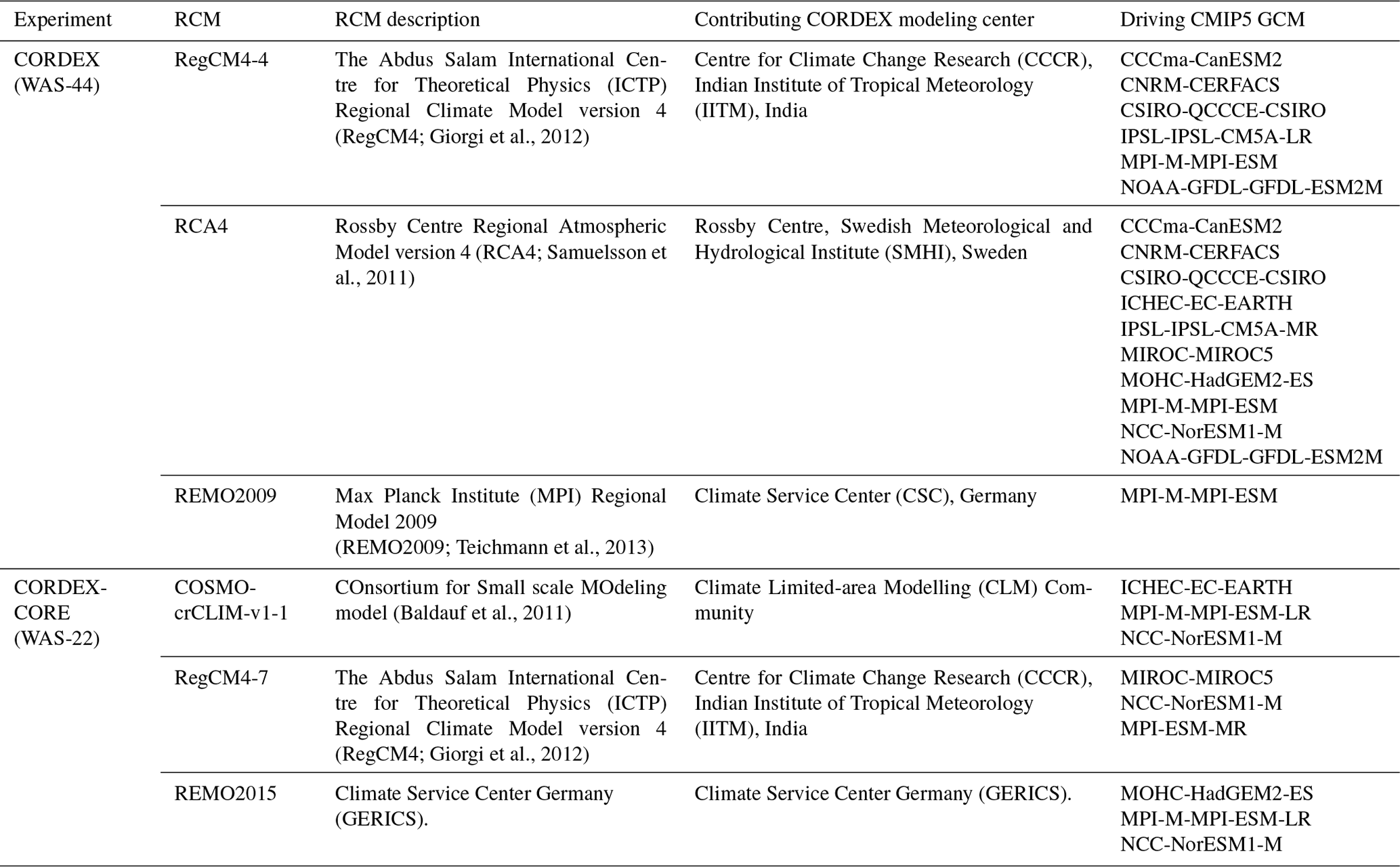
In the present work, we consider climate model historical simulations from 2 GCMs of the 6th Coupled Intercomparison Project (CMIP6; Eyring et al., 2016), 17 RCM simulations (3 RCMs unevenly driven by 10 GCMs) of the Coordinated Regional Climate Downscaling Experiment (CORDEX; Giorgi et al., 2009; Jones, 2010), and 9 RCM simulations (3 RCMs unevenly driven by 6 GCMs) of the CORDEX Coordinated Output for Regional Evaluations (CORDEX-CORE; Teichmann et al., 2021). For the RCM simulations, the South Asian domain (denoted as WAS) is considered. In particular, we use all available simulations by November 2021 for WAS-44 and WAS-22 domains (simulations conducted at horizontal resolutions of 0.44∘ and 0.22∘ on rotated grids, approximately 50 and 25 km) for CORDEX and for CORDEX-CORE, respectively. The selection of this particular subset of GCMs from CMIP6 is motivated by the availability of models with high spatial resolution (Table 1), approximately similar to the CORDEX counterparts. Coarser GCMs are not considered due to the small size of the catchment under study. More details on the considered climate models are given in Tables 1 and 2.
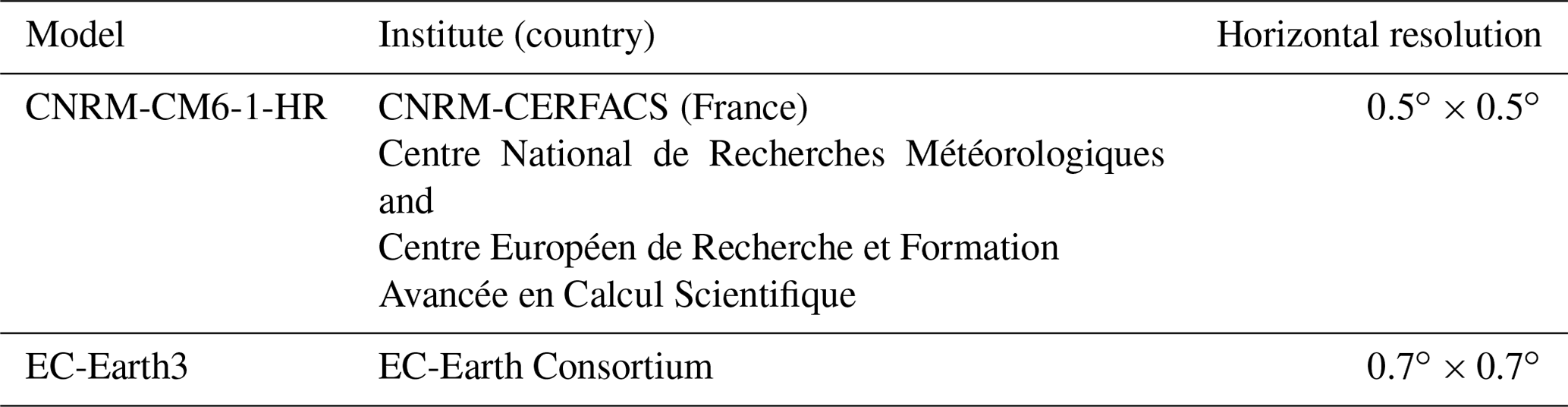
Table 2Details of the CORDEX and CORDEX-CORE RCMs used in the present study.
2.5 Bias correction methods
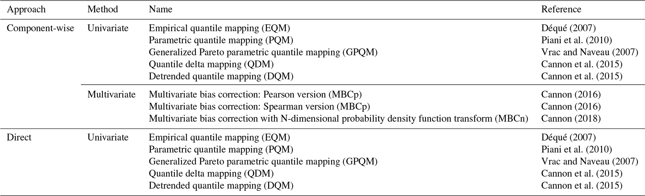
Several univariate and multivariate bias correction methods are used in this study. A comparison between five univariate bias correction methods and three multivariate bias correction methods is performed with respect to their ability to reproduce observed univariate distributions and inter-variable relationships. The univariate methods are applied to climate model simulations following two approaches: (1) individually to all involved essential climatic variables (i.e., the component-wise approach) and (2) directly to the uncorrected SPEI (i.e., the direct approach). All BC methods make a common assumption of stationary biases by applying the same calibrated transfer function in the calibration period (1986–2005) to the future projected climate which may lead to modifications of the raw model climate change signals for non-trend-preserving methods. The Table 3 summarizes the considered BC approaches and methods.
Table 3Bias correction approaches and methods employed in the present study.
2.5.1 Univariate bias correction methods
Five univariate methods (either parametric or empirical) are considered in this study. The present study uses the implementation included in the R package “downscaleR” (Bedia et al., 2020a) which is part of the R bundle “climate4R” (Iturbide et al., 2019).
-
Empirical quantile mapping (EQM). This method calibrates an empirical transfer function that matches all quantiles of the model empirical cumulative distribution function (CDF) to those of the reference dataset. The values lying outside the calibration range are adjusted through constant extrapolation (first and last percentile corrections for values below and above the calibration range, respectively) (Themeßl et al., 2012). The method also adjusts the overestimation of wet or dry day frequency (defined as days with precipitation above or below 1 mm in the reference dataset) in the model using, respectively, adjusted wet-day threshold and frequency adaptation proposed by Themeßl et al. (2012) and Wilcke et al. (2013). If a model produces too many wet days, then the wet-day frequency is corrected in such a way that it matches the observed wet-day frequency. In the case of the overestimation of dry days in the model, then the frequency adaptation is made through the random sampling of the observed gamma distribution into the simulated first bin (0–1 mm) in order to generate wet days.
-
Parametric quantile mapping (PQM). This method adjusts the theoretical CDF of the model output onto the corresponding observed distribution via a parametric transfer function calibrated over the training period (Piani et al., 2010). Assumptions are made about the distribution of a particular variable (i.e., precipitation and temperature follow the gamma and Gaussian distributions, respectively). As for EQM, in the considered implementation the overestimation of wet or dry days in the model data is also adjusted using wet-day frequency correction and the frequency adaptation approach, respectively.
-
Generalized Pareto parametric quantile mapping (GPQM). The method is specifically designed to adjust the extremes of the distribution. It fits two different parametric distributions to adjust the extreme and non-extreme values separately. The gamma or Gaussian distribution (for precipitation and temperature, respectively) adjusts the central part, whereas generalized Pareto distributions are applied above the 95th and below 5th percentiles (Vrac and Naveau, 2007). As for EQM, the wet-day frequency correction and frequency adaptation are applied.
-
The Quantile Delta Mapping (QDM). The method was first developed by Li et al. (2010) and Wang and Chen (2014) as “equidistant” and “equiratio” quantile matching, respectively. The main idea is to preserve the trends of all quantiles of the simulated distribution. Later, Cannon et al. (2015) termed both methods as QDM due to its similarity to a quantile delta change method. Firstly, model projections are detrended by quantile, and quantile mapping is applied to adjust systematic distributional biases relative to the observations. Then the removed projected trends are reintroduced to the bias-corrected quantiles. Thus, it ensures that the sensitivity of the underlying climate model remains unaffected by the bias correction (at least so far as quantiles are concerned).
-
Detrended quantile mapping (DQM). The method is similar to QDM, except that absolute or relative changes in the simulated mean are accounted for rather than all modeled quantiles (Cannon et al., 2015). Hence, the long-term mean (linear) trend is removed, and bias correction is applied to the detrended series by empirical quantile mapping using all quantiles to adjust systematic distributional biases relative to observation. Then the mean trend is reintroduced to the bias-corrected series. As DQM only preserves long-term mean trends, it does not ensure that the simulated model trends at the tails of the distribution that define climate extremes are preserved (Casanueva et al., 2020).
2.5.2 Multivariate bias correction methods
The three MBC methods used to adjust the inter-variable structure in this study are MBCp, MBCr (Cannon, 2016), and MBCn (Cannon, 2018). The MBCp and MBCr methods are the combination of two approaches: firstly, quantile delta mapping is applied to each variable individually in order to correct the marginal distribution of the variables including the preservation of absolute (in the case of temperature) or relative (in the case of non-Gaussian variables like precipitation) raw climate change signal, and, secondly, multivariate linear rescaling is applied (Bürger et al., 2011) in order to adjust the dependence structure through an iterative application of the Cholesky decomposition of the covariance matrix. The Pearson correlation and Spearman rank correlation are used as the covariance matrix in the MBCp and MBCr methods, respectively. These two steps are repeated until both the marginal distributions and specified correlation matrix converge to those of the reference dataset.
The MBCn algorithm, which is based on the N-dimensional probability density function transform, is adopted from an image processing algorithm used to transfer color information (Pitie et al., 2005; Pitié et al., 2007). Unlike the MBCp and MBCr methods, MBCn permits us to transfer all statistical characteristics of the observed multivariate distribution to those of the climate model outputs. In MBCn, random orthogonal rotation matrices are applied to the observed and climate model data to partially decorrelate the climate variables before the QDM. It is then rotated back with the inverse random matrices. The processes of rotation, QDM, and back rotation are repeated iteratively until the multivariate distribution of the historical climate model data converges to that of the reference data. In the present study, the MBCn algorithm is iterated 30 times to get the bias-corrected output. The present study uses the implementation included in the R package “MBC” (https://cran.r-project.org/web/packages/MBC, last access: August 2022).
2.6 Experimental framework
In this study, the BC methods presented above are applied to adjust daily maximum temperature, minimum temperature, and precipitation of 28 (global and regional) climate model simulations (Tables 1 and 2) towards the W5E5 reference dataset. All BC methods are calibrated in the period 1986–2005 using daily time series, the correction functions being calculated separately for each month in order to account for biases varying throughout the year. These corrections are then applied to the same period on a monthly basis in order to evaluate their performance in the present climate. Although the calibration and evaluation periods are the same, our approach can be considered independent since the evaluated aspect (i.e., SPEI indices) is not directly adjusted by the BC methods. All analyses are carried out at the spatial resolution of the W5E5 grid (regular 50 × 50 km). For this reason, all model simulations are remapped into the W5E5 grid. For this purpose, CORDEX-CORE simulations are conservatively remapped into the observational grid in order to guarantee the representation of areal averages. For CMIP6 and CORDEX simulations, the nearest-neighbor grid box to each observational grid box is taken, since the resolution mismatch is small. This interpolation method maintains the higher spatial variability in the topographical areas, whereas bilinear or cubic interpolation would smooth the spatial patterns. As a consequence, there will be aspects of the added value of the higher-resolution WAS-22 experiments (related to better-resolved, fine-scale processes) that can be smoothed out, but they may still be present after remapping them onto a coarse resolution. Thus, we address the added value of the high resolution at its skillful scale (Grasso, 2000), which is coarser than the scale in which the simulation was developed.
For all BC methods, daily maximum temperatures, minimum temperature, and precipitation from each GCM and RCM are corrected independently at each grid box. Due to the multivariate nature of the SPEI, daily maximum temperature, minimum temperature, and precipitation are corrected separately (in the case of univariate BC methods) and jointly (in the case of multivariate BC methods) prior to the SPEI calculation (i.e., the component-wise approach; Casanueva et al., 2018). An alternative to this approach is to first calculate the SPEI from the original, biased simulations (i.e., original modeled inter-variable relationships remain) and, secondly, bias-correct the index itself using univariate methods (direct approach; Casanueva et al., 2018). Note that a normal distribution is assumed for the direct correction of the SPEI through the PQM method. In addition to the evaluation of the performance of BC methods and approaches, the added value of higher spatial resolution in the modeled data (CORDEX-CORE over CORDEX and CMIP6) is assessed. Both assessments are performed in terms of the ability to simulate the mean spatiotemporal distribution of the SPEI and its derived indices over the study region.
2.7 Evaluation metrics
The performance of the raw and bias-corrected climate model simulations (component-wise approach) is firstly evaluated in terms of univariate indices related to temporal aspects not calibrated specifically by any of the BC methods. For this purpose, we consider indices defined by the EU-COST Action VALUE (Maraun et al., 2019), representing day-to-day characteristics (transition probability of a wet day given that the previous day was dry, longest dry spell, and longest warm spell) and monthly and annual features (amplitude of the annual cycle and interannual variance). Secondly, we evaluated inter-variable relationships by using two statistical metrics, namely the correlation coefficient (Pearson, 1895; Wilks, 2011) and Perkins skill score (Perkins et al., 2007). The correlation coefficient between daily time series of two variables (Spearman for Pr vs. Tmax and Pr vs. Tmin and Pearson for Tmax vs. Tmin) is computed at each grid cell to measure the relationship between pairs of variables. Since Pearson and Spearman correlation coefficients imply a linear and nonlinear relationship, respectively, they are hence recommended for temperature and precipitation, respectively (Wilcke et al., 2013). The Perkins skill score is a quantitative measure of the similarity between two probability density functions (PDFs) by measuring the common area between them. A value of 0 indicates no overlap, and a value of 1 indicates distributions are identical. In the present study, an extended version of the Perkins skill score with two dimensions is used that accounts for the similarity (overlap) between the modeled joint distribution of two meteorological variables and the observed counterpart (Casanueva et al., 2019). Further, the raw and bias-corrected climate model data (component-wise and direct approaches) are evaluated by using the mean bias (ratio of model to reference) of the SPEI indices (median duration, median severity, and absolute frequency; see Sect. 2.2).
3.1 Evaluation of temporal properties
The ability of the BC methods to represent the marginal properties of the individual variables is expected, since they are related to parameters which have been calibrated by the methods explicitly (Casanueva et al., 2016). They might, however, deteriorate temporal properties, as is the case for multivariate BC methods (e.g., François et al., 2020), since they have not been adjusted by any of the methods. Figures S1–S5 in the Supplement show the overall improvement in temporal properties after BC, with a systematic reduction in model biases and no clear benefit of multivariate methods. Raw models present an overall overestimation of dry-to-wet transition probability, which is reduced after BC especially for QDM, MBCn, and MBCp (Fig. S1). Annual longest dry and warm spells are underestimated and overestimated, respectively, in the raw models, and biases are largely corrected after most BC methods. Overall, DQM presents the largest departures from the reference dataset. The above-mentioned statistics and their inadequate representation in the BC data might lead to biases in the SPEI, which relies on daily values of the input variables. Similar conclusions hold for temporal properties at longer timescales, such as the amplitude of the annual cycle (Fig. S2) and interannual variance (Figs. S3–S5). The amplitude of the annual cycle is largely improved by most BC methods, except for the annual cycle of precipitation which is overestimated by GPQM and underestimated by DQM (Fig. S2). The interannual variance for monthly precipitation is well represented after BC, except for the overestimation by GPQM in some months (Fig. S3). The large overestimation of the interannual variance of maximum and minimum temperatures is not completely solved by BC, since important overestimations remain for all BC methods (Figs. S4–S5).
3.2 Evaluation of inter-variable relationships
To evaluate the inter-variable structures, the correlation coefficient (COR) and the Perkins skill score (PSS) between daily maximum and minimum temperatures are computed at each grid cell to measure the relationship between the two physical variables (Fig. 1). The heat map shows the spatially averaged values of Pearson correlation (size of the marker) and Perkins skill score (colored scale) for the raw and bias-corrected model output; i.e., the larger the marker is, the stronger the relationship between the two variables is, and the yellower the color is, the more similar the joint PDFs are to the reference dataset. The Spearman correlation coefficient between the other pairs of variables (Pr vs. Tmax and Pr vs. Tmin) for the reference dataset is found to be negligible (Fig. S6). Therefore, the ability of the BC methods to adjust the inter-variable dependencies is evaluated only for maximum and minimum temperature. Note that we focus on inter-variable relationships at daily timescales, since this is when they are expected to be relevant for the SPEI used in the present work. However, more important correlations between precipitation and temperatures are found at the monthly scale in the reference data (up to −0.54; Fig. S7), which are not present in most of the raw models but are improved after BC (except for GPQM; Fig. S8).
Overall, small differences in terms of correlation are found for raw and bias-corrected model outputs compared to the reference value (Fig. 1). Maximum and minimum temperature showed a strong positive correlation exceeding 0.9 in W5E5, which is also evident in the raw models and preserved after BC. However, one climate simulation (REMO2009 RCM driven by the MPI GCM) shows a weaker correlation for the raw model output and improves with all BC methods.
Regarding PSS, low values for the raw model outputs show the differences in the joint PDF of Tmax and Tmin compared to the reference data, meaning that the inter-variable dependencies in the reference dataset are not well presented by the raw model output. However, this inter-variable physical coherence improves to some extent with the application of all BC methods. Among univariate BC methods, the empirical ones (EQM, DQM, and QDM) performed better than the parametric counterparts in terms of the inter-variable physical coherence between maximum and minimum temperature. As expected, all MBC methods performed well and improve upon the univariate ones. Among three MBC methods, MBCn outperformed the other two methods, with a very similar joint PDF to the reference data.
All the above holds for most of the different climate model simulations, regardless of the RCM, driving GCM, original spatial resolution (CORDEX vs. CORDEX-CORE), and modeling experiment (CMIP vs. CORDEX). Although the differences among different climate model simulations from three modeling experiments exist for parametric methods (PQM and GPQM), no specific pattern is found. Thus, no evident added value of the higher-resolution experiment models (WAS-22) is observed over low-resolution experiment models (WAS-44 and CMIP6) in either correlation or Perkins skill score. However, a clear added value of multivariate BC methods is apparent.
To further explore the ability of raw and BC datasets to reproduce the reference full joint probability distribution of maximum temperature and minimum temperature, two-dimensional kernel density plots, together with marginal histograms (Fig. 2), are developed for a single grid box of an RCM (highlighted red box in Figs. 1 and 2). The selection of this particular grid box is motivated by the low values of correlation and PSS for the raw simulation and subsequent improvement after BC in order to investigate whether low PSS values can be attributed to biases in maximum temperature, minimum temperature, or both. Higher density values in the reference dataset (Fig. 2, first row and second column) take place around 20 and 7 ∘C for maximum and minimum temperature, respectively. For the raw model output, the shape and location of the joint distribution and maximum probability are biased at both ends of the distributions, as evident in the low PSS value, i.e., 0.641. This low PSS value of the raw simulation is attributed to both variables but especially to the misrepresentation of the minimum temperature distribution. Likewise, the temporal correlation between the two variables is slightly lower than in the reference. Correlation and PSS improve after BC regardless of the BC method with the least improvement in the joint distribution with GPQM (PSS = 0.707). Higher density values are located well with parametric methods, i.e., PQM and GPQM (this would be expected because they fit the mean and standard deviation in the calibration phase), but for GPQM they are not so differentiated as in the reference data. The other three univariate BC methods (i.e., EQM, DQM, and QDM) and multivariate methods improve the representation of the joint distribution in a similar way, although maxima are not so differentiated as in the reference data.
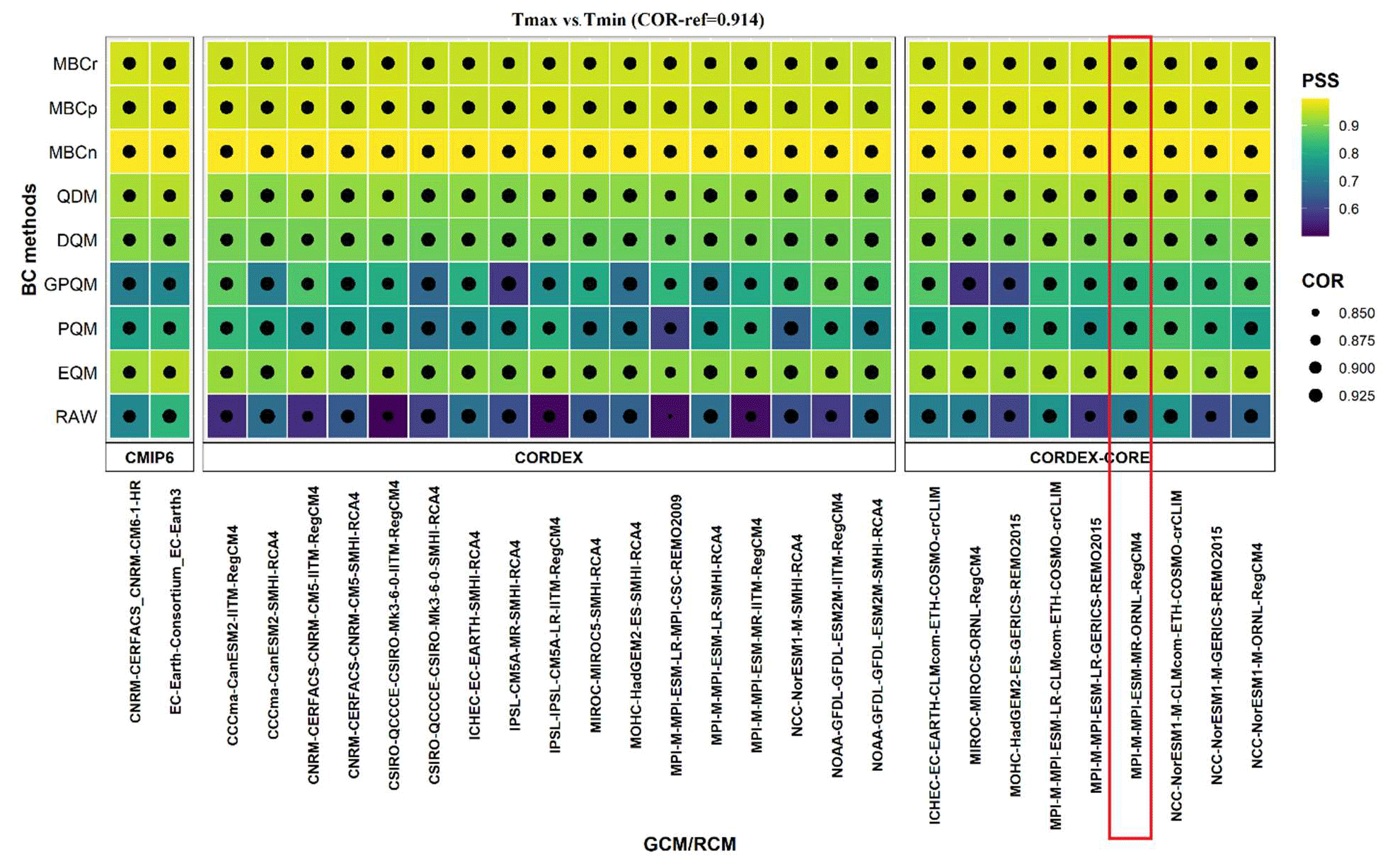
Figure 1Pearson correlation coefficient (COR, circle) between maximum and minimum temperatures and Perkins skill score (PSS, colored scale) of the joint PDFs for the raw and bias-corrected climate model data (only component-wise approach). The correlation for the reference dataset is shown at the top of the figure. The highlighted RCM (red square) is selected for further analyses in Fig. 2.
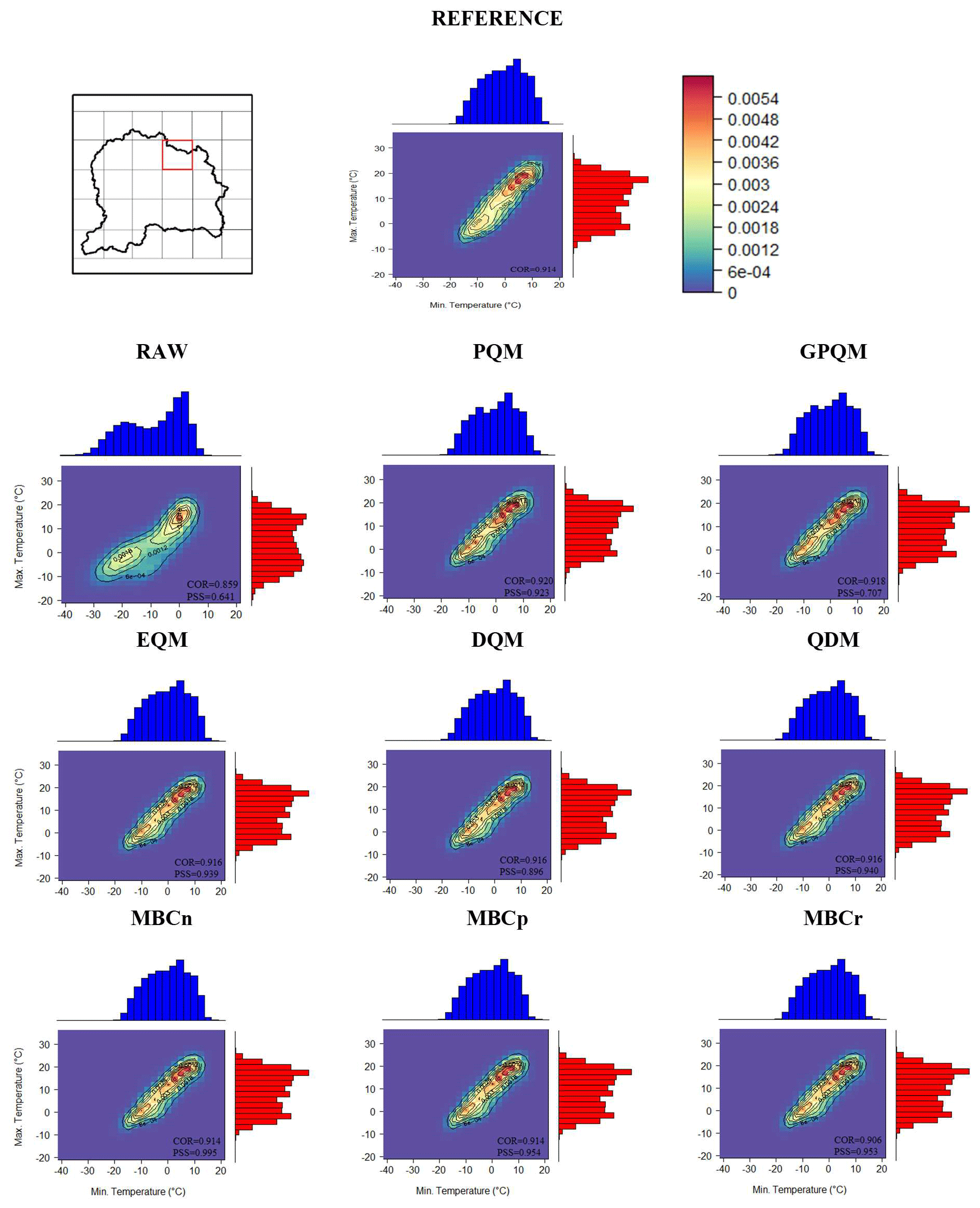
Figure 2Two-dimensional kernel density plots for the highlighted grid box (red box). Blue histograms (and x axis) refer to minimum temperature, and red histograms (and y axis) refer to maximum temperature. Shadings represent the two-dimensional density distribution for the reference, raw, and eight BC methods. Contour lines represent the probabilities in the reference dataset, which are overlaid on the model probabilities for the sake of comparison. COR depicts the Pearson correlation coefficient between daily minimum and maximum temperatures, and PSS represents the two-dimensional Perkins skill score of distributional similarity.
3.3 Evaluation of SPEI characteristics
The performance of the raw and bias-corrected climate model simulations is evaluated in terms of mean biases (ratio of model to reference dataset) in SPEI indices (duration, severity, and frequency; see Sect. 2.2) during the historical period (1986–2005). The spatial distributions of biases calculated from multi-model ensemble mean SPEI indices, separately for CMIP6 (2 simulations), CORDEX (17), and CORDEX-CORE (9), are presented in Figs. 3–4 and S9–S12. Results show that the northeast part of the region, located at the foothills of the Western Himalayas, is found to be more affected by wet and dry events with higher severity and duration (see the upper left panel in each figure). The higher susceptibility of the region towards more extreme events could be explained with the increasing rates of global warming over mountainous region, i.e., Western Himalayas, also reported by many researchers (Pachauri et al., 2014; Zaz et al., 2019; Rashid et al., 2020; Shafiq et al., 2020; Ansari and Grossi, 2022). Studies by Negi et al. (2018) and Dimri and Dash (2012) also confirm that most of the Western Himalayan region recorded a significant warming trend especially from 1975 onwards. This is also supported by the tree-ring chronologies of the region which indicate rapid growth of the tree rings in the recent decades especially at higher altitudes (Borgaonkar et al., 2009).
In the context of biases, different sign biases are found depending on the location and SPEI. The underestimation of all SPEI indices is higher in the northeast part of the region, which shows that raw climate models' performance is relatively poor over mountainous regions. Overall, larger biases are found in frequency indices compared to duration and severity indices. These under- and overestimations are partly alleviated by most of the bias correction methods. Regarding severity indices (Figs. 3 and 4), remaining biases after BC are similar across BC methods, with an underestimation of WS in the mountainous region and no specific pattern for DS. In the case of duration indices (Figs. S9 and S10), the overestimation in the lowlands is improved by all BC methods; however, that improvement is not only negligible, but it also degrades the raw CMIP6 ensemble in the northeast of the basin (mountainous region). The underestimation of frequency indices over high mountains (Figs. S11 and S12) is partially reduced by all BC methods with slightly better performance under the direct approach. However, bias correction induces an overestimation in WF over lowlands which is not present in raw ensembles of all datasets. Overall, GPQM is found to bring the least improvement for most of the SPEI indices, and the added value of MBC methods is not evident in the remaining univariate methods.
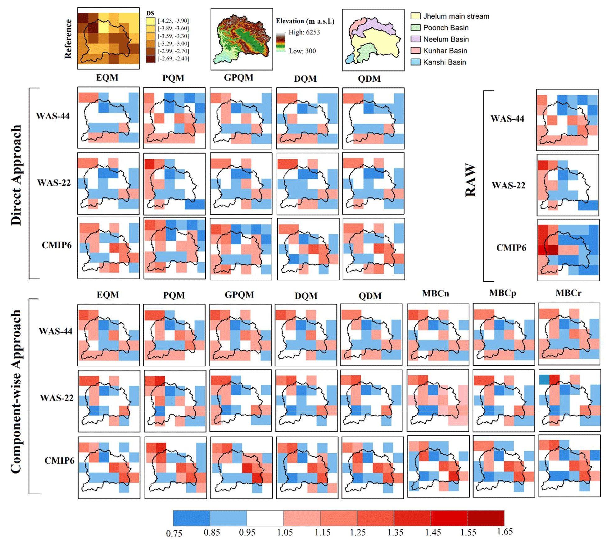
Figure 3Median dry severity (DS) in the reference dataset expressed in accumulated SPEI units (first row, left), digital elevation model in meters above sea level (first row, center) and location of sub-basins (first row, right), and biases (as a ratio of model to reference) of DS for the multi-model raw and bias-corrected ensembles for the two bias correction approaches and all methods (columns).
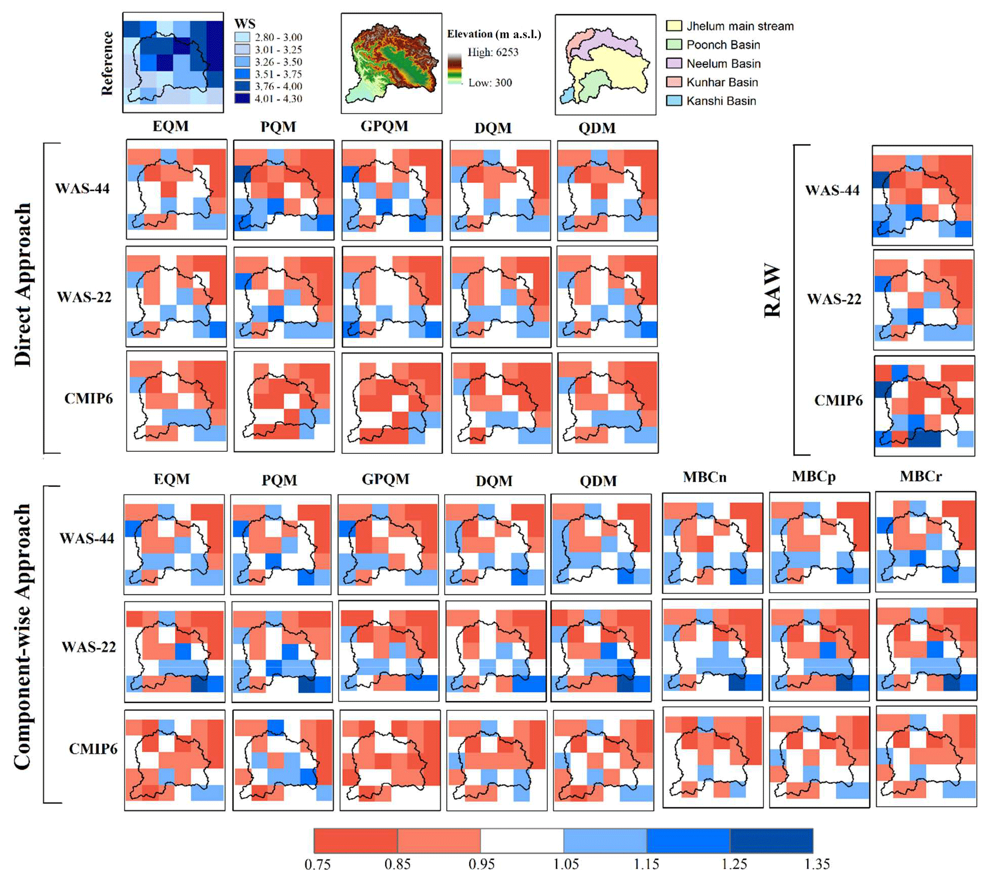
Figure 4Same as Fig. 3 but for median wet severity (WS), expressed in accumulated SPEI units.
The regionally averaged biases in median duration and severity and the absolute frequency of dry and wet events for all individual climate simulations (CORDEX-CORE, CORDEX, and CMIP6) are summarized in Fig. 5. Overall, results show that raw models generally underestimate all SPEI indices, and bias correction alleviates this for frequency and severity indices, but shorter events than in the reference dataset are found after the corrections. The conclusions drawn from the spatial plots also relate to climate models' spread. For instance, the small improvement in duration indices over high mountains is in line with a slight reduction in the model spread after bias correction, yet the underestimation of the DD and WD remains. Similarly, for WF the reduction in the underestimation over high mountains and increase in the overestimation over lowlands by all BC methods are in agreement with changes in the models' spread after bias correction (Figs. S12 and 5).
In general, all BC methods under the direct approach present similar improvements for all SPEI indices, except PQM for dry extremes which shows smaller improvements for some simulations. Regarding the component-wise approach, the empirical BC methods, i.e., EQM, DQM, and QDM, performed relatively better than PQM and GPQM for most of the models and SPEI indices. Small differences are found in the performance of three MBC methods.
Regarding the spatial resolution, no obvious benefit of the higher resolution (CORDEX-CORE vs. CORDEX and CMIP6) is apparent. Raw model outputs from CORDEX-WAS44 show more spread than the CMIP6 and CORDEX-CORE experiment models, which could be due to the number of simulations. After BC, the spread of CORDEX and CORDEX-CORE is similar, and thus, no clear added value of higher resolution is found.
Overall, the performance of BC methods and climate models is found to be relatively better for drought indices than for flood indices. Most of the models underestimate wet duration and severity over the region before and after bias correction.
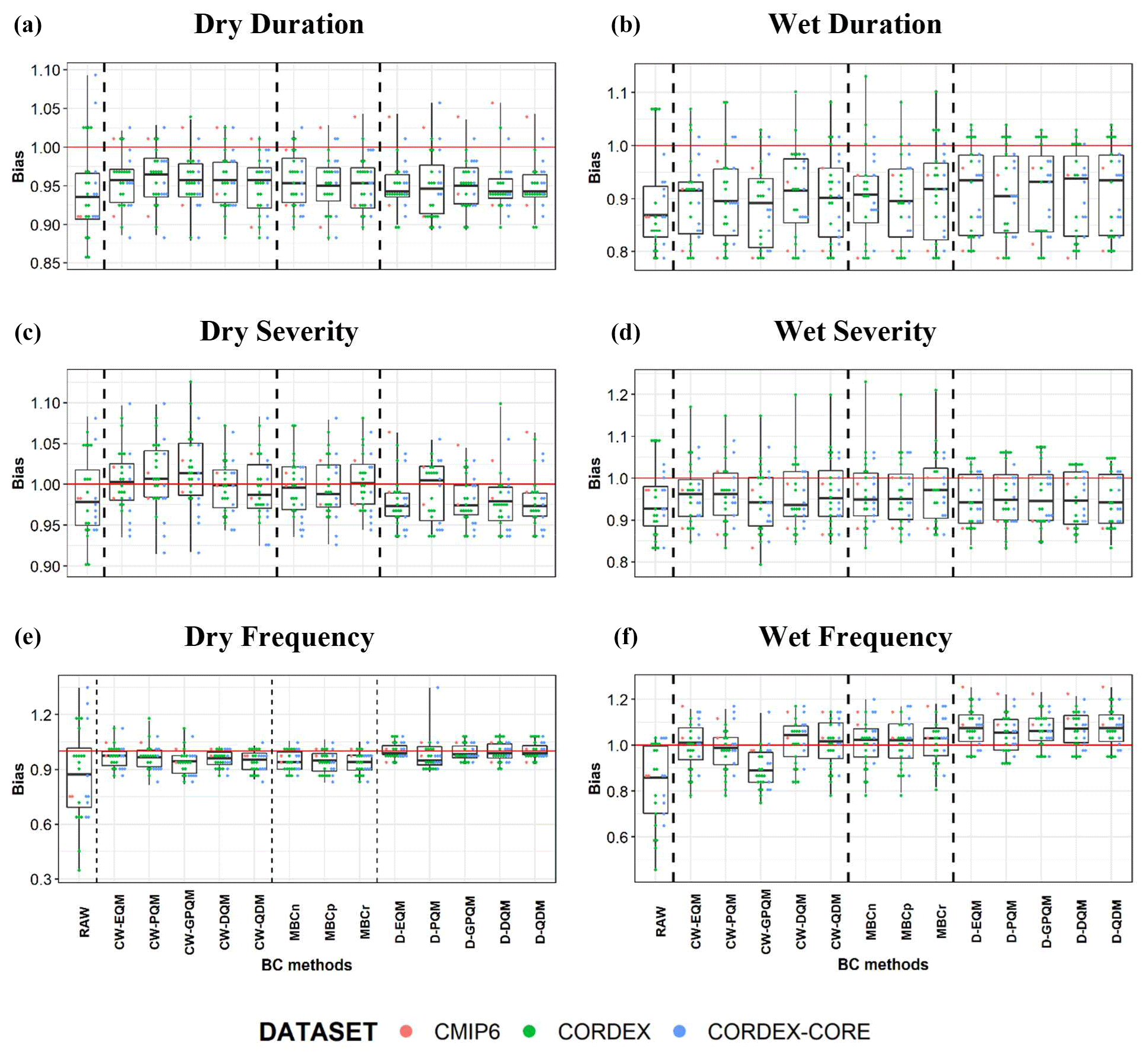
Figure 5Biases (as a ratio of model to reference) in spatially averaged SPEI indices over Upper Jhelum Basin computed from the raw (first box in each panel) and bias-corrected data (rest of the boxes; CW: component-wise; D: direct). Each box represents the interquartile range of biases across all models, which are depicted individually with colored dots (CMIP6 in red, CORDEX in green, CORDEX-CORE in blue), and whiskers expand the full range of biases. Horizontal red lines depict perfect performance, for reference.
3.4 Effect of bias correction on the spatial pattern of SPEI characteristics
The ability of the BC methods under both approaches to represent the spatial structure of SPEI indices (median duration and severity and absolute frequency of dry and wet events) in the historical period (1986–2005) for the UJB is explored by Taylor diagrams (Fig. 6). These Taylor diagrams (Taylor, 2001) show the degree of agreement between the spatial pattern of raw and bias-corrected data and the observed counterpart for SPEI indices by means of spatial Pearson correlation coefficient (dotted lines), (centered) root mean square error (blue curves), and normalized standard deviation (black curve denotes perfect performance). Note that correlations below 0.5 might not be statistically significant given the small sample size (30 grid boxes; Bujang and Baharum, 2016).
The Taylor diagrams indicate that overall, all BC methods improve upon the raw model output for all datasets and SPEI indices. The correlation coefficient is much lower for duration and severity SPEI indices (typically lies between 0.1 and 0.8), whereas it amounts to between 0.5 and 0.9 for WF and over 0.8 for DF. Concerning the normalized standard deviation (nSD) most of the bias-corrected results underestimate the spatial variability in all SPEI indices. This underestimation amounts up to 50 % (nSD between 0.5 to 1.0) except for WD and DF, which show maximum and minimum underestimation, respectively. The centered root mean square errors between BC and reference SPEI indices are found to be in the range of 0.3 to 1.2, the lowest being for frequency indices especially for DF (0.3 to 0.6). Overall, the spatial pattern for the frequency SPEI indices indicates better agreement with the reference dataset than for the duration and severity SPEI indices for most of the BC methods and datasets.
The performance of BC methods is rather consistent for most of the SPEI indices regardless of the statistical measure (i.e., correlation coefficient, normalized standard deviation, and centered root mean square error). More specifically, all BC methods under the direct approach show better agreement than the component-wise approach for most of the SPEI indices and datasets. The EQM, PQM, and QDM under the direct approach are grouped together for all SPEI indices and datasets. For the component-wise approach, no systematic difference between the best-performing univariate methods and the multivariate ones is found.
Regarding the spatial resolution of the original model data, no clear benefit of the higher resolution (CORDEX-CORE vs. CORDEX and CMIP6) is found, and results vary with the SPEI indices and depend more on the BC method than on the model ensemble. The degree of agreement of CORDEX and CORDEX-CORE experiments with reference data is comparable, and they tend to group together for the frequency indices; however, differences exist with CMIP6 models. For the best-performing BC methods, the CORDEX ensemble presents the largest correlation and smallest root mean square error for dry events and WD, whereas the CORDEX-CORE ensemble represents better the spatial variability. For the dry SPEI indices, CMIP6 falls behind both CORDEX experiments, even for the best-performing BC methods. For WS, most datasets present correlation coefficients of 0.4–0.6, and the spatial variability is larger for CORDEX-CORE and CMIP6. For WF, datasets group by BC method regardless of the model ensemble. Note that here the multi-model ensemble mean is considered, which might hinder the potential added value of individual simulations.
To further explore the inner-ensemble variability and potential added value of individual simulations of CORDEX and CORDEX-CORE experiments, Fig. 7 shows the performance of bias-corrected (using D-EQM) individual climate model simulations from the two experiments. Interestingly, there is no clear best-performing driving GCM or RCM for all SPEI indices, and large discrepancies in the reference data remain for some individual simulations after bias correction. In general, CORDEX simulations show a higher correlation coefficient and smaller root mean square error, and CORDEX-CORE presents more accurate spatial variability. The RCM and GCM combination also matters. For example, the performance of REMO2015 is poor when driven by MPI (which is its typical driving GCM), but it is one of the best with HadGEM2 for most of the indices. On the other hand, the HadGEM2-driven RCM in the CORDEX-CORE experiment (REMO2015) performed well compared to in the CORDEX experiment (RCA4). Similarly, the added value of higher spatial resolution (CORDEX-CORE over CORDEX) can also be seen with RegCM4 driven by MPI in both experiments (filled and non-filled dark brown circle). However, the added value of the CORDEX-CORE experiment does not hold for all simulation pairs. For instance, NorESM1-driven RCMs in both experiments do not show a clear behavior (filled and non-filled dark green shapes).

Figure 6Taylor diagrams showing the performance of BC methods (colors) and datasets (markers) with respect to the spatial variability in the SPEI indices in the historical period (1986–2005) for the UJB. Each marker represents the evaluation measures for the multi-model ensemble mean SPEI indices for the three modeling experiments (CORDEX in circles, CORDEX-CORE in triangles, CMIP6 in diamonds). Filled markers: direct BC approach; non-filled markers: component-wise BC approach; black marker: raw model output. Note: in the case of CMIP6, D-EQM (filled grey diamond) and D-PQM (filled dark blue diamond) are grouped together for all SPEI indices. Note: in the case of CMIP6, D-QDM (filled pink diamond) and D-DQM (filled dark green diamond) are grouped together for all SPEI indices. Note: in the case of CORDEX and CORDEX-CORE experiments, D-EQM (filled grey marker), D-PQM (filled dark-blue marker), and D-QDM (filled pink marker) are grouped together for all SPEI indices.
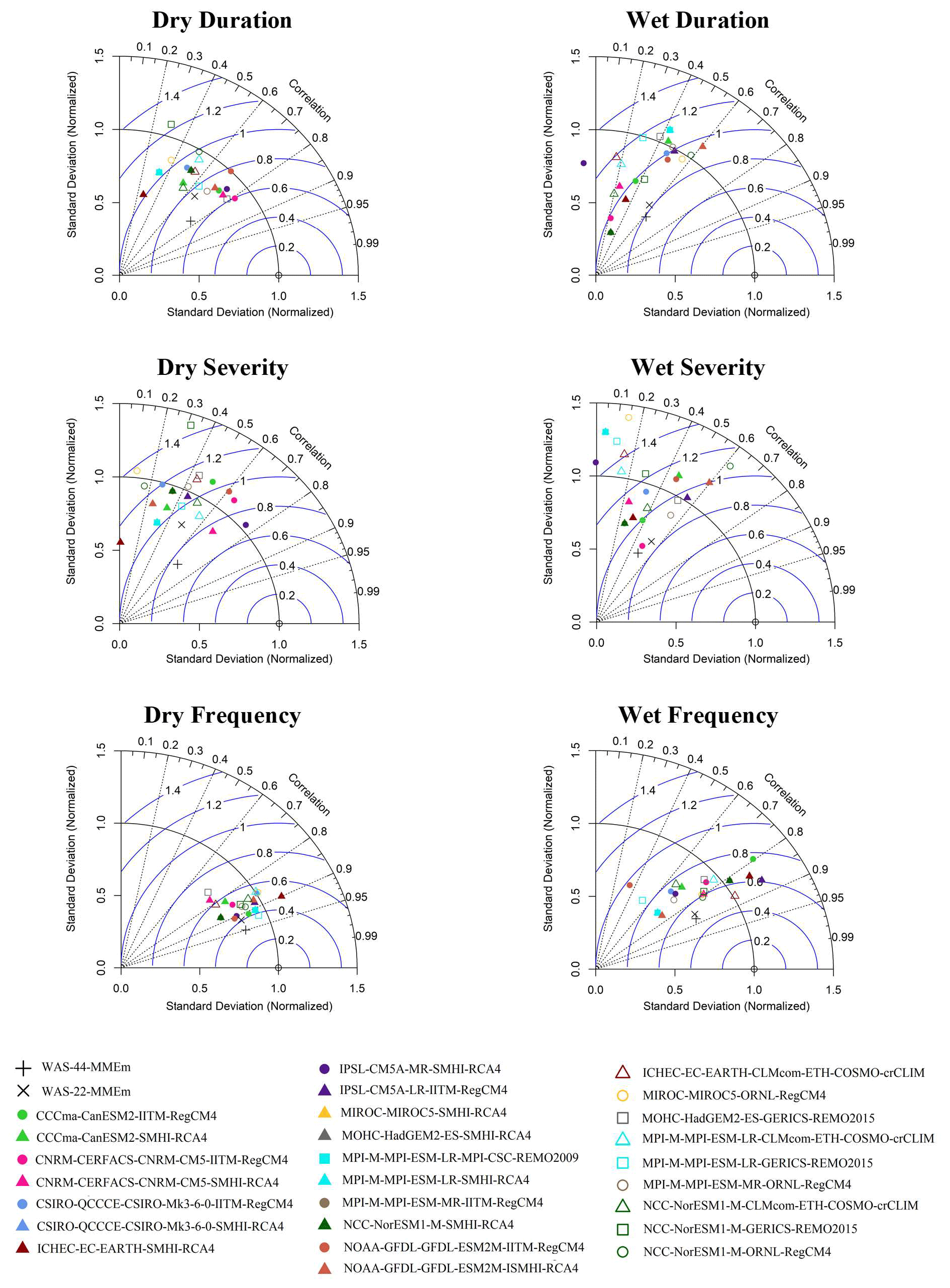
Figure 7Taylor diagrams showing the performance of individual simulations of CORDEX and CORDEX-CORE experiments bias-corrected using the D-EQM method with respect to the spatial pattern of SPEI indices in the historical period (1986–2005) for the UJB. Filled markers: CORDEX models; non-filled markers: CORDEX-CORE models. Three different markers show the three RCMs in both experiments (i.e., RegCM4, RCA4, and REMO2009 from CORDEX and COSMO, and REMO2015 and RegCM4-7 from CORDEX-CORE); colors show the driving GCMs (same color means same driving GCM); plus marker and cross in black show the multi-model ensemble mean (MMEm) for CORDEX and CORDEX-CORE experiments, respectively. Note: RCA4 driven by CSIRO (filled blue triangle) and ICHEC-EC-EARTH (filled maroon triangle) are grouped together for all SPEI indices. Note: RCA4 driven by MIROC (filled yellow triangle), RCA4 driven by MOHC-HadGEM2 (filled grey triangle), RCA4 driven by MPI (filled cyan triangle), and REMO2009 driven by MPI (filled cyan square) are grouped together for all SPEI indices. Note: RegCM4 driven by MPI (filled brown circle) and RCA4 driven by NCC-NorESM1 (filled dark green triangle) are grouped together.
This study assesses the performance of two BC approaches (direct and component-wise) and eight methods (univariate and multivariate) for an impact-relevant, multivariate drought index (SPEI) that characterizes wet and dry extreme events over the Upper Jhelum Basin in the Western Himalayas.
From obtained results, most of the univariate BC methods under both direct and component-wise approaches exhibit a comparable performance in the current climate, with a slightly better performance for the direct approach. The direct approach with univariate methods also provides comparable results to more sophisticated multivariate methods, which could be due to the weak relationship among the input variables of the SPEI in this region at daily timescales. The spatial pattern is better reproduced by the direct approach than the component-wise approach (see Taylor diagrams in Sect. 3.4). This is expected from the experimental design, since under the direct approach, the SPEI is corrected as a single variable, regardless of the biases in the input essential climatic variables and in their interdependencies. Concerning univariate methods, the performance of parametric methods (i.e., PQM and GPQM) is found to be the worst especially in terms of inter-variable physical dependencies. Among the univariate empirical BC methods, both QDM and DQM exhibit a similar performance for the SPEI indices and inter-variable physical dependencies. Regarding the performance multivariate BC methods, all methods show comparable performance. Overall, the best-performing univariate (i.e., empirical) methods are comparable to the multivariate ones. Overall, biases are reduced with all BC methods to some extent, but still SPEI indices are not well resolved. Reasons for this could be the remaining biases after BC in temporal properties of the individual variables (Figs. S1–S5 in the Supplement), which have not been calibrated by any of the methods, together with the nonlinear, multivariate nature of the SPEI, which is not directly calibrated by BC either.
Findings on the limited performance of a few univariate BC methods, especially parametric (PQM and GPQM), under both approaches are admittedly based on the inadequate representation of temporal properties and inter-variable physical relationships. The direct correction of the SPEI using univariate BC methods that does not consider the dependencies between variables has the advantage of adjusting a single variable instead of several variables with different statistical properties, and in this work it shows slightly better performance than correcting individual climatic variables prior to the SPEI calculation. Nevertheless, the advantages of the direct approach over the component-wise approach, the multivariate over univariate BC methods, and the trend-preserving over non-trend-preserving methods still need to be evaluated for the projected future conditions (Casanueva et al., 2018). Moreover, our findings may differ from other multivariate hazard or impact-related indices in different regions of the world. Since the individual variables in a multivariate hazard index are interlinked differently, the contribution of their individual biases to the associated multivariate hazard index may lead to different results. For instance, biases in wet-bulb globe temperature (WBGT) are found to be smaller than in the Chandler burning index (CBI) for a given model output, yet both indices are based on temperature and relative humidity (Villalobos-Herrera et al., 2021). This is attributed to the construction of the index, since bias in CBI is mainly driven by the bias in relative humidity, whereas bias in WBGT interplays between biases in temperature and relative humidity, which compensate each other.
Contrasting conclusions are found in the literature about the added value of multivariate BC methods over univariate ones in impact-relevant studies. For example, Guo et al. (2020) reported the regionally dependent added value of MBC methods over univariate methods in reproducing observed inter-variable dependencies and observed streamflow using the GR4J hydrological model. Similar findings also have been identified with the Canadian fire weather index (Cannon, 2018), heat stress (WBGT) and fire risk (CBI) indicators (Zscheischler et al., 2019), and snowmelt-driven streamflow (Meyer et al., 2019). On the other hand, Eum et al. (2020) reported marginal improvements in MBC methods in reproducing the extreme climatic indices and hydrological indicators over Alberta, Canada. Räty et al. (2018) also indicated that it is difficult to demonstrate that multivariate methods may significantly reduce biases in hydrologic indicators. Van de Velde et al. (2022) stated that the simpler univariate BC methods are better to use for climate change impact assessment, as the MBC methods failed to handle non-stationary climate conditions. François et al. (2020) reported the added value of multivariate BC methods over univariate ones and concluded that also multivariate methods can deteriorate temporal aspects and that the choice of the BC method should be based on the end user's goal. In the present study, the added value of multivariate BC methods over univariate ones is only evident for inter-variable physical coherence, whereas comparable results are found in terms of biases in temporal properties and SPEI indices. The comparable performances for SPEI indices could be attributed to the weak relationship among the input variables (precipitation and temperature) of the SPEI in this region for the daily timescale and to biased temporal properties. In comparison to the direct BC approach, Chen et al. (2021) found a similar performance of MBC and the direct correction of hydrological model output, i.e., streamflow in the present climate; however, both are sensitive to non-stationary biases during the validation period. They recommended the MBC especially for streamflow projections under a strong anthropogenic signature on the climate. They also reported that biases in streamflow simulations depend on the climate model output, hydrological model, streamflow metrics, and region. Similar conclusions were also made by Casanueva et al. (2018), who state that the direct correction of the Canadian fire weather index (FWI) presents a similar performance to the FWI calculated from individually corrected climate variables in the present climate but found a more robust behavior for the component-wise approach under future climate change.
The added value of higher climate model resolution (CORDEX-CORE vs. CORDEX and CMIP6) is not evident in the evaluation step in terms of either inter-variable physical coherence or SPEI indices. There is some indication of added value of CORDEX-CORE with respect to CORDEX and CMIP6 in terms of the representation of spatial variability. However, the CORDEX ensemble performs best in terms of correlation and root mean square error in the spatial patterns. Nevertheless, the absence of obvious benefits of a finer grid resolution in the present work does not rule out such an added value in general. For instance, a study conducted by Maharana et al. (2021) on Indian summer monsoon precipitation found improved representation of mean precipitation in individual CORDEX-CORE models from the CORDEX experiment. Moreover, the 0.5∘ resolution of the gridded observational reference (W5E5), coarser than that of the 0.22∘ CORDEX-CORE simulations, allows us to draw conclusions concerning a lack of large-scale bias improvements by the 0.22∘ CORDEX-CORE experiments but hinders the identification of benefits at a smaller scale. The added value of finer spatial resolution could be more obvious if the evaluation is carried out at the original resolution (Prein et al., 2016; Casanueva et al., 2019) especially for the processes over complex terrains where abrupt orographic changes cause much larger spatial variability. Although the uncertainty due to the spatial resolution of the reference dataset is out of the scope of the present study due to limited availability of reliable finer-resolution observational datasets for the studied region, many other studies acknowledge its greater impact especially for extreme precipitation indices (Casanueva et al., 2019, 2020). Kotlarski et al. (2014) also stated that the obvious added value of finer-resolution simulations over its coarser counterpart is strongly dependent on the availability and accessibility of fine-gridded and high-quality observational datasets.
To summarize, there is some added value of multivariate bias correction with respect to univariate BC methods in the representation of the inter-variable structures, but comparable results to the best-performing univariate BC methods are found in terms of biases in SPEI indices. Present climate evaluation shows limited added value of higher-spatial-resolution simulations mainly due to the experimental design (both resolutions are remapped onto the 50 × 50 km observational grid). Future work will explore to what extent current results of bias correction are robust under projected climate. Moreover, the application of bias-corrected climate model outputs to identify geographical hotspots prone to wet and dry extreme events, as well as their temporal compounding under different warming levels, will be very useful for stakeholders (researchers, local authorities, policy makers, relief agencies, non-governmental organizations (NGOs), and (re-)insurance companies) working on potential risk and the associated development of adaptation strategies to climate change in this region.
All calculations and plots were produced using R (version 3.3.2) and ArcMap (version 10.8) by making use of open-source R packages. For univariate bias correction, the present study uses the implementation included in the R package “downscaleR” (version 3.3.3) which is part of the R bundle “climate4R” (Bedia et al., 2020a; Iturbide et al., 2019) available from a GitHub repository (https://github.com/SantanderMetGroup/downscaleR, last access: August 2022, https://doi.org/10.5281/zenodo.5070432, Bedia et al., 2020b). R package “MBC” version 0.10-5 (https://rdocumentation.org/packages/MBC/versions/0.10-5) is used for the multivariate bias correction methods (Cannon, 2018, 2016; Cannon et al., 2015). The potential evapotranspiration (PET) and standardized precipitation evapotranspiration index (SPEI) were calculated with the R package “SPEI” (version 1.7) available from a GitHub repository (https://github.com/sbegueria/SPEI, last access: August 2022, Beguería et al., 2017). All the code to perform the derived analyses, calculations, and plots is also based on R scripts and ArcMap, which are available at https://doi.org/10.5281/zenodo.7296744 (Ansari et al., 2022a).
The reference data (W5E5) are available for download at https://doi.org/10.5880/PIK.2019.023 (Lange, 2019), and the climate model simulations from three initiatives (CORDEX, CORDEX-CORE, and CMIP6) used in this study are accessible via the Earth System Grid Federation (ESGF archive; https://esgf.llnl.gov, last access: August 2022; Earth System Grid Federation, 2022). ESGF is not a dataset but a multi-agency, international collaboration that aims at developing the software infrastructure needed to facilitate and empower the study of climate phenomena on a global scale. ESGF consists of several nodes distributed around the globe, most of which are maintained by European and North American institutions. By accessing the ESGF link one can connect to one node, search for data, and download them.
The supplement related to this article is available online at: https://doi.org/10.5194/gmd-16-2055-2023-supplement.
RA, AC, and GG conceptualized the study. RA performed the formal analyses. AC gave support regarding the bias correction methods and model data, and MUL provided ideas for new analyses and illustrations. GG and AC supervised the work. RA wrote the first draft of the paper, and all authors reviewed the text and contributed to the final version.
The contact author has declared that none of the authors has any competing interests.
Publisher’s note: Copernicus Publications remains neutral with regard to jurisdictional claims in published maps and institutional affiliations.
The authors acknowledge the World Climate Research Programme's Working Group on Regional Climate and the Working Group on Coupled Modelling, the former coordinating body of CORDEX and panel responsible for CMIP5. We also thank the climate modeling groups (listed in Tables 1 and 2 of this paper) for producing and making available their model output. We also acknowledge the Earth System Grid Federation infrastructure, an international effort led by the U.S. Department of Energy's Program for Climate Model Diagnosis and Intercomparison, the European Network for Earth System Modelling, and other partners in the Global Organisation for Earth System Science Portals (GO-ESSP). Data were accessed through the Santander Climate Data Service, which is maintained by the Santander Meteorology Group. The authors are also grateful to Ezequiel Cimadevilla (Santander Meteorology Group) for technical support. We are also grateful to two anonymous reviewers for their constructive comments.
This research has been supported by the cooperation agreement PFK PhD program 2019–2022 “Partnership for Knowledge-Platform 2: Health and WASH (WAter Sanitation and good Hygiene)” of the AICS-Italian Agency for Development Cooperation, the Erasmus Traineeship Program, Project COMPOUND (TED2021-131334A-I00) funded by MCIN/AEI/10.13039/501100011033 and by the European Union NextGenerationEU/PRTR, and the Horizon 2020 project IS-ENES3 (grant agreement no. 824084).
This paper was edited by Sophie Valcke and reviewed by two anonymous referees.
Addor, N., Rohrer, M., Furrer, R., and Seibert, J.: Propagation of biases in climate models from the synoptic to the regional scale: Implications for bias adjustment, J. Geophys. Res.-Atmos., 121, 2075–2089, 2016.
Allen, R. G., Pereira, L. S., Raes, D., and Smith, M.: Crop Evapotranspiration-Guidelines for computing crop water requirements-FAO Irrigation and drainage paper 56, FAO, Rome, 300, D05109, https://www.fao.org/3/x0490e/x0490e00.htm (last access: August 2022), ISBN 92-5-104219-5, 1998.
Ansari, R. and Grossi, G.: Spatio-temporal evolution of wet–dry event features and their transition across the Upper Jhelum Basin (UJB) in South Asia, Nat. Hazards Earth Syst. Sci., 22, 287–302, https://doi.org/10.5194/nhess-22-287-2022, 2022.
Ansari, R., Casanueva, A., Liaqat, M. U., and Grossi, G.: Climate change projections of wet and dry extreme events in the Upper Jhelum Basin using a multivariate drought index: Evaluation of bias correction, Zenodo [code], https://doi.org/10.5281/zenodo.7296744, 2022a.
Ansari, R., Liaqat, M. U., and Grossi, G.: Evaluation of gridded datasets for terrestrial water budget assessment in the Upper Jhelum River Basin-South Asia, J. Hydrol., 613, 128294, https://doi.org/10.1016/j.jhydrol.2022.128294, 2022b.
Argüeso, D., Evans, J. P., and Fita, L.: Precipitation bias correction of very high resolution regional climate models, Hydrol. Earth Syst. Sci., 17, 4379–4388, https://doi.org/10.5194/hess-17-4379-2013, 2013.
Arshad, M., Ma, X., Yin, J., Ullah, W., Liu, M., and Ullah, I.: Performance evaluation of ERA-5, JRA-55, MERRA-2, and CFS-2 reanalysis datasets, over diverse climate regions of Pakistan, Weather and Climate Extremes, 33, 100373, https://doi.org/10.1016/j.wace.2021.100373, 2021.
Azmat, M., Qamar, M. U., Huggel, C., and Hussain, E.: Future climate and cryosphere impacts on the hydrology of a scarcely gauged catchment on the Jhelum river basin, Northern Pakistan, Sci. Total Environ., 639, 961–976, 2018.
Baldauf, M., Seifert, A., Förstner, J., Majewski, D., Raschendorfer, M., and Reinhardt, T.: Operational convective-scale numerical weather prediction with the COSMO model: Description and sensitivities, Mon. Weather Rev., 139, 3887–3905, 2011.
Baudouin, J.-P., Herzog, M., and Petrie, C. A.: Cross-validating precipitation datasets in the Indus River basin, Hydrol. Earth Syst. Sci., 24, 427–450, https://doi.org/10.5194/hess-24-427-2020, 2020.
Bedia, J., Baño-Medina, J., Legasa, M. N., Iturbide, M., Manzanas, R., Herrera, S., Casanueva, A., San-Martín, D., Cofiño, A. S., and Gutiérrez, J. M.: Statistical downscaling with the downscaleR package (v3.1.0): contribution to the VALUE intercomparison experiment, Geosci. Model Dev., 13, 1711–1735, https://doi.org/10.5194/gmd-13-1711-2020, 2020a.
Bedia, J., Baño-Medina, J., Legasa, M. N., Iturbide, M., Manzanas, R., Herrera, S., Casanueva, A., San-Martín, D., Cofiño, A. S., and Gutiérrez, J. M.: SantanderMetGroup/downscaleR: v3.3.3 (05 Jul 2021), v3.3.3, Zenodo [code], https://doi.org/10.5281/zenodo.5070432, 2020b.
Beguería, S., Vicente-Serrano, S. M., Reig, F., and Latorre, B.: Standardized precipitation evapotranspiration index (SPEI) revisited: parameter fitting, evapotranspiration models, tools, datasets and drought monitoring, Int. J. Climatol., 34, 3001–3023, 2014.
Beguería, S., Vicente-Serrano, S. M., and Beguería, M. S.: Package “SPEI”. Calculation of the Standardised Precipitation-Evapotranspiration Index, CRAN [code], https://github.com/sbegueria/SPEI (last access: August 2022), 2017.
Borgaonkar, H., Ram, S., and Sikder, A.: Assessment of tree-ring analysis of high-elevation Cedrus deodara D. Don from Western Himalaya (India) in relation to climate and glacier fluctuations, Dendrochronologia, 27, 59–69, 2009.
Bujang, M. A. and Baharum, N.: Sample size guideline for correlation analysis, World, 3, 37–46, 2016.
Bürger, G., Schulla, J., and Werner, A.: Estimates of future flow, including extremes, of the Columbia River headwaters, Water Resour. Res., 47, W10520, https://doi.org/10.1029/2010WR009716, 2011.
Cannon, A. J.: Multivariate bias correction of climate model output: Matching marginal distributions and intervariable dependence structure, J. Climate, 29, 7045–7064, 2016.
Cannon, A. J.: Multivariate quantile mapping bias correction: an N-dimensional probability density function transform for climate model simulations of multiple variables, Clim. Dynam., 50, 31–49, 2018.
Cannon, A. J., Sobie, S. R., and Murdock, T. Q.: Bias correction of GCM precipitation by quantile mapping: How well do methods preserve changes in quantiles and extremes?, J. Climate, 28, 6938–6959, https://doi.org/10.1175/JCLI-D-14-00754.1, 2015 (data available at: https://rdocumentation.org/packages/MBC/versions/0.10-5, last access: August 2022).
Casanueva, A., Frías, M. D., Herrera, S., San-Martín, D., Zaninovic, K., and Gutiérrez, J. M.: Statistical downscaling of climate impact indices: testing the direct approach, Climatic Change, 127, 547–560, 2014.
Casanueva, A., Herrera, S., Fernández, J., and Gutiérrez, J. M.: Towards a fair comparison of statistical and dynamical downscaling in the framework of the EURO-CORDEX initiative, Climatic Change, 137, 411–426, 2016.
Casanueva, A., Bedia, J., Herrera, S., Fernández, J., and Gutiérrez, J. M.: Direct and component-wise bias correction of multi-variate climate indices: the percentile adjustment function diagnostic tool, Climatic Change, 147, 411–425, 2018.
Casanueva, A., Kotlarski, S., Herrera, S., Fischer, A. M., Kjellstrom, T., and Schwierz, C.: Climate projections of a multivariate heat stress index: the role of downscaling and bias correction, Geosci. Model Dev., 12, 3419–3438, https://doi.org/10.5194/gmd-12-3419-2019, 2019.
Casanueva, A., Herrera, S., Iturbide, M., Lange, S., Jury, M., Dosio, A., Maraun, D., and Gutiérrez, J. M.: Testing bias adjustment methods for regional climate change applications under observational uncertainty and resolution mismatch, Atmos. Sci. Lett., 21, e978, https://doi.org/10.1002/asl.978, 2020.
Chen, J., Li, C., Brissette, F. P., Chen, H., Wang, M., and Essou, G. R.: Impacts of correcting the inter-variable correlation of climate model outputs on hydrological modeling, J. Hydrol., 560, 326–341, 2018.
Chen, J., Arsenault, R., Brissette, F. P., and Zhang, S.: Climate Change Impact Studies: Should We Bias Correct Climate Model Outputs or Post-Process Impact Model Outputs?, Water Resour. Res., 57, e2020WR028638, https://doi.org/10.1029/2020WR028638, 2021.
Christensen, J. H., Boberg, F., Christensen, O. B., and Lucas-Picher, P.: On the need for bias correction of regional climate change projections of temperature and precipitation, Geophys. Res. Lett., 35, L20709, https://doi.org/0.1029/2008GL035694, 2008.
Cucchi, M., Weedon, G. P., Amici, A., Bellouin, N., Lange, S., Müller Schmied, H., Hersbach, H., and Buontempo, C.: WFDE5: bias-adjusted ERA5 reanalysis data for impact studies, Earth Syst. Sci. Data, 12, 2097–2120, https://doi.org/10.5194/essd-12-2097-2020, 2020.
Dahri, Z. H., Ludwig, F., Moors, E., Ahmad, B., Khan, A., and Kabat, P.: An appraisal of precipitation distribution in the high-altitude catchments of the Indus basin, Sci. Total Environ., 548, 289–306, 2016.
Déqué, M.: Frequency of precipitation and temperature extremes over France in an anthropogenic scenario: Model results and statistical correction according to observed values, Global Planet. Change, 57, 16–26, 2007.
Dimri, A. and Dash, S.: Wintertime climatic trends in the western Himalayas, Climatic Change, 111, 775–800, 2012.
Droogers, P. and Allen, R. G.: Estimating reference evapotranspiration under inaccurate data conditions, Irrigation and Drainage Systems, 16, 33–45, 2002.
Earth System Grid Federation: https://esgf.llnl.gov/, last access: August 2022.
Eden, J. M., Widmann, M., Grawe, D., and Rast, S.: Skill, correction, and downscaling of GCM-simulated precipitation, J. Climate, 25, 3970–3984, 2012.
Ehret, U., Zehe, E., Wulfmeyer, V., Warrach-Sagi, K., and Liebert, J.: HESS Opinions “Should we apply bias correction to global and regional climate model data?”, Hydrol. Earth Syst. Sci., 16, 3391–3404, https://doi.org/10.5194/hess-16-3391-2012, 2012.
Eum, H.-I., Gupta, A., and Dibike, Y.: Effects of univariate and multivariate statistical downscaling methods on climatic and hydrologic indicators for Alberta, Canada, J. Hydrol., 588, 125065, https://doi.org/10.1016/j.jhydrol.2020.125065, 2020.
Eyring, V., Bony, S., Meehl, G. A., Senior, C. A., Stevens, B., Stouffer, R. J., and Taylor, K. E.: Overview of the Coupled Model Intercomparison Project Phase 6 (CMIP6) experimental design and organization, Geosci. Model Dev., 9, 1937–1958, https://doi.org/10.5194/gmd-9-1937-2016, 2016.
François, B., Vrac, M., Cannon, A. J., Robin, Y., and Allard, D.: Multivariate bias corrections of climate simulations: which benefits for which losses?, Earth Syst. Dynam., 11, 537–562, https://doi.org/10.5194/esd-11-537-2020, 2020.
Giorgi, F., Jones, C., and Asrar, G. R.: Addressing climate information needs at the regional level: the CORDEX framework, World Meteorological Organization (WMO) Bulletin, World Meteorological Organization 2009, 58, 175–183, ref.29, 2009.
Giorgi, F., Coppola, E., Solmon, F., Mariotti, L., Sylla, M., Bi, X., Elguindi, N., Diro, G., Nair, V., and Giuliani, G.: RegCM4: model description and preliminary tests over multiple CORDEX domains, Clim. Res., 52, 7–29, 2012.
Grasso, L. D.: The differentiation between grid spacing and resolution and their application to numerical modeling, B. Am. Meteorol. Soc., 81, 579–580, 2000.
Guo, Q., Chen, J., Zhang, X. J., Xu, C. Y., and Chen, H.: Impacts of using state-of-the-art multivariate bias correction methods on hydrological modeling over North America, Water Resour. Res., 56, e2019WR026659, https://doi.org/10.1029/2019WR026659, 2020.
Gutiérrez, J. M., Jones, R. G., Narisma, G. T., Alves, L. M., Amjad, M., Gorodetskaya, I. V., Grose, M., Klutse, N. A. B., Krakovska, S., Li, J., Martínez-Castro, D., Mearns, L. O., Mernild, S. H., Ngo-Duc, T., van den Hurk, B., and Yoon, J.-H.: Atlas, in: Climate Change 2021: The Physical Science Basis. Contribution of Working Group I to the Sixth Assessment Report of the Intergovernmental Panel on Climate Change, edited by: Masson-Delmotte, V., Zhai, P., Pirani, A., Connors, S. L., Péan, C., Berger, S., Caud, N., Chen, Y., Goldfarb, L., Gomis, M. I., Huang, M., Leitzell, K., Lonnoy, E., Matthews, J. B. R., Maycock, T. K., Waterfield, T., Yelekçi, O., Yu, R., and Zhou, B., Cambridge University Press, Cambridge, United Kingdom and New York, NY, USA, 1927–2058, https://doi.org/10.1017/9781009157896.021, 2021.
Haerter, J. O., Hagemann, S., Moseley, C., and Piani, C.: Climate model bias correction and the role of timescales, Hydrol. Earth Syst. Sci., 15, 1065–1079, https://doi.org/10.5194/hess-15-1065-2011, 2011.
Hao, Z., Phillips, T. J., Hao, F., and Wu, X.: Changes in the dependence between global precipitation and temperature from observations and model simulations, Int. J. Climatol., 39, 4895–4906, 2019.
Hargreaves, G. H. and Samani, Z. A.: Reference crop evapotranspiration from temperature, Appl. Eng. Agric., 1, 96–99, 1985.
Hersbach, H., Bell, B., Berrisford, P., Hirahara, S., Horányi, A., Muñoz-Sabater, J., Nicolas, J., Peubey, C., Radu, R., and Schepers, D.: The ERA5 global reanalysis, Q. J. Roy. Meteor. Soc., 146, 1999–2049, 2020.
Himayoun, D. and Roshni, T.: Spatio-temporal variation of drought characteristics, water resource availability and the relation of drought with large scale climate indices: a case study of Jhelum basin, India, Quatern. Int., 525, 140–150, 2019.
Huang, C., Zhang, Q., Singh, V. P., Gu, X., and Shi, P.: Spatio-temporal variation of dryness/wetness across the Pearl River basin, China, and relation to climate indices, Int. J. Climatol., 37, 318–332, 2017.
Iturbide, M., Bedia, J., Herrera, S., Baño-Medina, J., Fernández, J., Frías, M. D., Manzanas, R., San-Martín, D., Cimadevilla, E., and Cofiño, A. S.: The R-based climate4R open framework for reproducible climate data access and post-processing, Environ. Modell. Softw., 111, 42–54, 2019.
Jones, C.: CORDEX: A Coordinated Regional Downscaling Experiment, AGU Fall Meeting Abstracts, A23F-01, December 2010, American Geophysical Union, Fall Meeting 2010, abstract id. A23F-01, 2010.
Kopp, R., Easterling, D. R., Hall, T., Hayhoe, K., Horton, R., Kunkel, K., and LeGrande, A.: Potential surprises – compound extremes and tipping elements, in: Climate Science Special Report: A Sustained Assessment Activity of the U.S. Global Change Research Program, edited by: Wuebbles, D. J., Fahey, D. W., Hibbard, K. A., Dokken, D. J., Stewart, B. C., and Maycock, T. K., U.S. Global Change Research Program, Washington, DC, USA, 608–635, https://digitalcommons.unl.edu/usdeptcommercepub/578 (last access: August 2022), 2017.
Kotlarski, S., Keuler, K., Christensen, O. B., Colette, A., Déqué, M., Gobiet, A., Goergen, K., Jacob, D., Lüthi, D., van Meijgaard, E., Nikulin, G., Schär, C., Teichmann, C., Vautard, R., Warrach-Sagi, K., and Wulfmeyer, V.: Regional climate modeling on European scales: a joint standard evaluation of the EURO-CORDEX RCM ensemble, Geosci. Model Dev., 7, 1297–1333, https://doi.org/10.5194/gmd-7-1297-2014, 2014.
Lange, S.: WFDE5 over land merged with ERA5 over the ocean (W5E5). V. 1.0, GFZ Data Services [data set], https://doi.org/10.5880/pik.2019.023, 2019.
Li, H., Sheffield, J., and Wood, E. F.: Bias correction of monthly precipitation and temperature fields from Intergovernmental Panel on Climate Change AR4 models using equidistant quantile matching, J. Geophys. Res.-Atmos., 115, D10101, https://doi.org/10.1029/2009JD012882, 2010.
Li, W., Chen, J., Li, L., Chen, H., Liu, B., Xu, C.-Y., and Li, X.: Evaluation and bias correction of S2S precipitation for hydrological extremes, J. Hydrometeorol., 20, 1887–1906, 2019.
Liaqat, M. U., Grossi, G., and Ranzi, R.: Characterization of interannual and seasonal variability of hydro-climatic trends in the Upper Indus Basin, Theor. Appl. Climatol., 147, 1163–1184, 2022.
Lutz, A. F., Immerzeel, W. W., Kraaijenbrink, P. D., Shrestha, A. B., and Bierkens, M. F.: Climate change impacts on the upper Indus hydrology: sources, shifts and extremes, PloS one, 11, e0165630, https://doi.org/10.1371/journal.pone.0165630, 2016.
Maharana, P., Kumar, D., Das, S., and Tiwari, P. R.: Present and future changes in precipitation characteristics during Indian summer monsoon in CORDEX-CORE simulations, Int. J. Climatol., 41, 2137–2153, 2021.
Mahony, C. R. and Cannon, A. J.: Wetter summers can intensify departures from natural variability in a warming climate, Nat. Commun., 9, 783, https://doi.org/10.1038/s41467-018-03132-z, 2018.
Maraun, D., Shepherd, T. G., Widmann, M., Zappa, G., Walton, D., Gutiérrez, J. M., Hagemann, S., Richter, I., Soares, P. M., and Hall, A.: Towards process-informed bias correction of climate change simulations, Nat. Clim. Change, 7, 764–773, 2017.
Maraun, D., Widmann, M., and Gutiérrez, J. M.: Statistical downscaling skill under present climate conditions: A synthesis of the VALUE perfect predictor experiment, Int. J. Climatol., 39, 3692–3703, 2019.
Maru, H., Haileslassie, A., Zeleke, T., and Esayas, B.: Agroecology-based analysis of meteorological drought and mapping its hotspot areas in Awash Basin, Ethiopia, Model. Earth Syst. Environ., 8, 339–360, https://doi.org/10.1007/s40808-021-01101-y, 2022.
Mavromatis, T.: Drought index evaluation for assessing future wheat production in Greece, Int. J. Climatol., 27, 911–924, 2007.
Meyer, J., Kohn, I., Stahl, K., Hakala, K., Seibert, J., and Cannon, A. J.: Effects of univariate and multivariate bias correction on hydrological impact projections in alpine catchments, Hydrol. Earth Syst. Sci., 23, 1339–1354, https://doi.org/10.5194/hess-23-1339-2019, 2019.
Naz, B. S., Kao, S.-C., Ashfaq, M., Gao, H., Rastogi, D., and Gangrade, S.: Effects of climate change on streamflow extremes and implications for reservoir inflow in the United States, J. Hydrol., 556, 359–370, 2018.
Negi, H., Kanda, N., Shekhar, M., and Ganju, A.: Recent wintertime climatic variability over the North West Himalayan cryosphere, Current Science, 114, 760–770, 2018.
Pachauri, R. K., Allen, M. R., Barros, V. R., Broome, J., Cramer, W., Christ, R., Church, J. A., Clarke, L., Dahe, Q., and Dasgupta, P.: Climate change 2014: synthesis report. Contribution of Working Groups I, II and III to the fifth assessment report of the Intergovernmental Panel on Climate Change, IPCC, hdl:10013/epic.45156.d001, 2014.
Pearson, K.: VII. Note on regression and inheritance in the case of two parents, P. R. Soc. London, 58, 240–242, 1895.
Perkins, S., Pitman, A., Holbrook, N. J., and McAneney, J.: Evaluation of the AR4 climate models' simulated daily maximum temperature, minimum temperature, and precipitation over Australia using probability density functions, J. Climate, 20, 4356–4376, 2007.
Piani, C., Haerter, J., and Coppola, E.: Statistical bias correction for daily precipitation in regional climate models over Europe, Theor. Appl. Climatol., 99, 187–192, 2010.
Pitie, F., Kokaram, A. C., and Dahyot, R.: N-dimensional probability density function transfer and its application to color transfer, in: Tenth IEEE International Conference on Computer Vision (ICCV'05), 17–21 October 2005, Beijing, China, IEEE, 1, 1434–1439, https://doi.org/10.1109/ICCV.2005.166, 2005.
Pitié, F., Kokaram, A. C., and Dahyot, R.: Automated colour grading using colour distribution transfer, Comput. Vis. Image Und., 107, 123–137, 2007.
Prein, A., Gobiet, A., Truhetz, H., Keuler, K., Goergen, K., Teichmann, C., Fox Maule, C., Van Meijgaard, E., Déqué, M., and Nikulin, G.: Precipitation in the EURO-CORDEX 0.11∘ and 0.44∘ simulations: high resolution, high benefits?, Clim. Dynam., 46, 383–412, 2016.
Rashid, I., Majeed, U., Aneaus, S., and Pelto, M.: Linking the recent glacier retreat and depleting streamflow patterns with land system changes in Kashmir Himalaya, India, Water, 12, 1168, https://doi.org/10.3390/w12041168, 2020.
Räty, O., Räisänen, J., Bosshard, T., and Donnelly, C.: Intercomparison of univariate and joint bias correction methods in changing climate from a hydrological perspective, Climate, 6, 33, https://doi.org/10.3390/cli6020033, 2018.
Raymond, C., Horton, R. M., Zscheischler, J., Martius, O., AghaKouchak, A., Balch, J., Bowen, S. G., Camargo, S. J., Hess, J., and Kornhuber, K.: Understanding and managing connected extreme events, Nat. Clim. Change, 10, 611–621, 2020.
Samuelsson, P., Jones, C. G., Willén, U., Ullerstig, A., Gollvik, S., Hansson, U., Jansson, E., Kjellström, C., Nikulin, G., and Wyser, K.: The Rossby Centre Regional Climate model RCA3: model description and performance, Tellus A, 63, 4–23, https://doi.org/10.1111/j.1600-0870.2010.00478.x, 2011.
Schmucki, E., Marty, C., Fierz, C., Weingartner, R., and Lehning, M.: Impact of climate change in Switzerland on socioeconomic snow indices, Theor. Appl. Climatol., 127, 875–889, 2017.
Shafiq, M. U., Islam, Z. U., Bhat, I. A., and Ahmed, P.: Spatio-temporal behaviour of Nehnar Glacier from 1962 to 2017, Jhelum basin, Kashmir Himalayas, India, Phys. Geogr., 41, 517–536, 2020.
Stevens, B. and Bony, S.: What are climate models missing?, Science, 340, 1053–1054, 2013.
Svoboda, M., Hayes, M., and Wood, D.: Standardized precipitation index: user guide, World Meteorological Organization (WMO-No. 1090), Geneva, ISBN 978-92-63-11090-9, 2012.
Taylor, K. E.: Summarizing multiple aspects of model performance in a single diagram, J. Geophys. Res.-Atmos., 106, 7183–7192, 2001.
Teichmann, C., Eggert, B., Elizalde, A., Haensler, A., Jacob, D., Kumar, P., Moseley, C., Pfeifer, S., Rechid, D., and Remedio, A. R.: How does a regional climate model modify the projected climate change signal of the driving GCM: a study over different CORDEX regions using REMO, Atmosphere, 4, 214–236, 2013.
Teichmann, C., Jacob, D., Remedio, A. R., Remke, T., Buntemeyer, L., Hoffmann, P., Kriegsmann, A., Lierhammer, L., Bülow, K., and Weber, T.: Assessing mean climate change signals in the global CORDEX-CORE ensemble, Clim. Dynam., 57, 1269–1292, 2021.
Teutschbein, C. and Seibert, J.: Bias correction of regional climate model simulations for hydrological climate-change impact studies: Review and evaluation of different methods, J. Hydrol., 456, 12–29, 2012.
Themeßl, M. J., Gobiet, A., and Heinrich, G.: Empirical-statistical downscaling and error correction of regional climate models and its impact on the climate change signal, Climatic Change, 112, 449–468, 2012.
Van de Velde, J., Demuzere, M., De Baets, B., and Verhoest, N. E. C.: Impact of bias nonstationarity on the performance of uni- and multivariate bias-adjusting methods: a case study on data from Uccle, Belgium, Hydrol. Earth Syst. Sci., 26, 2319–2344, https://doi.org/10.5194/hess-26-2319-2022, 2022.
Vicente-Serrano, S. M., Beguería, S., and López-Moreno, J. I.: A multiscalar drought index sensitive to global warming: the standardized precipitation evapotranspiration index, J. Climate, 23, 1696–1718, 2010.
Villalobos-Herrera, R., Bevacqua, E., Ribeiro, A. F. S., Auld, G., Crocetti, L., Mircheva, B., Ha, M., Zscheischler, J., and De Michele, C.: Towards a compound-event-oriented climate model evaluation: a decomposition of the underlying biases in multivariate fire and heat stress hazards, Nat. Hazards Earth Syst. Sci., 21, 1867–1885, https://doi.org/10.5194/nhess-21-1867-2021, 2021.
Vrac, M. and Naveau, P.: Stochastic downscaling of precipitation: From dry events to heavy rainfalls, Water Resour. Res., 43, W07402, https://doi.org/10.1029/2006WR005308, 2007.
Wang, L. and Chen, W.: Equiratio cumulative distribution function matching as an improvement to the equidistant approach in bias correction of precipitation, Atmos. Sci. Lett., 15, 1–6, 2014.
Wang, Q., Wu, J., Lei, T., He, B., Wu, Z., Liu, M., Mo, X., Geng, G., Li, X., and Zhou, H.: Temporal-spatial characteristics of severe drought events and their impact on agriculture on a global scale, Quatern. Int., 349, 10–21, 2014.
Wang, Q., Shi, P., Lei, T., Geng, G., Liu, J., Mo, X., Li, X., Zhou, H., and Wu, J.: The alleviating trend of drought in the Huang-Huai-Hai Plain of China based on the daily SPEI, Int. J. Climatol., 35, 3760–3769, 2015.
Weedon, G. P., Balsamo, G., Bellouin, N., Gomes, S., Best, M. J., and Viterbo, P.: The WFDEI meteorological forcing data set: WATCH Forcing Data methodology applied to ERA-Interim reanalysis data, Water Resour. Res., 50, 7505–7514, 2014.
Wilby, R. L., Hay, L. E., Gutowski Jr., W. J., Arritt, R. W., Takle, E. S., Pan, Z., Leavesley, G. H., and Clark, M. P.: Hydrological responses to dynamically and statistically downscaled climate model output, Geophys. Res. Lett., 27, 1199–1202, 2000.
Wilcke, R. A. I., Mendlik, T., and Gobiet, A.: Multi-variable error correction of regional climate models, Climatic Change, 120, 871–887, 2013.
Wilks, D. S.: Statistical methods in the atmospheric sciences, Academic Press, 3rd edn., International geophysics series, vol. 100, ISBN 978-0-12-385022-5, https://doi.org/10.1016/B978-0-12-385022-5.00001-4, 2011.
Yao, J., Zhao, Y., Chen, Y., Yu, X., and Zhang, R.: Multi-scale assessments of droughts: a case study in Xinjiang, China, Sci. Total Environ., 630, 444–452, 2018.
Zaz, S. N., Romshoo, S. A., Krishnamoorthy, R. T., and Viswanadhapalli, Y.: Analyses of temperature and precipitation in the Indian Jammu and Kashmir region for the 1980–2016 period: implications for remote influence and extreme events, Atmos. Chem. Phys., 19, 15–37, https://doi.org/10.5194/acp-19-15-2019, 2019.
Zscheischler, J., Westra, S., Van Den Hurk, B. J., Seneviratne, S. I., Ward, P. J., Pitman, A., AghaKouchak, A., Bresch, D. N., Leonard, M., and Wahl, T.: Future climate risk from compound events, Nat. Clim. Change, 8, 469–477, 2018.
Zscheischler, J., Fischer, E. M., and Lange, S.: The effect of univariate bias adjustment on multivariate hazard estimates, Earth Syst. Dynam., 10, 31–43, https://doi.org/10.5194/esd-10-31-2019, 2019.
Zscheischler, J., Martius, O., Westra, S., Bevacqua, E., Raymond, C., Horton, R. M., van den Hurk, B., AghaKouchak, A., Jézéquel, A., and Mahecha, M. D.: A typology of compound weather and climate events, Nature Reviews Earth & Environment, 1, 333–347, 2020.