the Creative Commons Attribution 4.0 License.
the Creative Commons Attribution 4.0 License.
 | 06 Apr 2023
Understanding AMOC stability: the North Atlantic Hosing Model Intercomparison Project
Laura C. Jackson
Eduardo Alastrué de Asenjo
Katinka Bellomo
Gokhan Danabasoglu
Helmuth Haak
Johann Jungclaus
Warren Lee
Virna L. Meccia
Oleg Saenko
Andrew Shao
Didier Swingedouw
The Atlantic meridional overturning circulation (AMOC) is an important part of our climate system. The AMOC is predicted to weaken under climate change; however, theories suggest that it may have a tipping point beyond which recovery is difficult, hence showing quasi-irreversibility (hysteresis). Although hysteresis has been seen in simple models, it has been difficult to demonstrate in comprehensive global climate models. Here, we outline a set of experiments designed to explore AMOC hysteresis and sensitivity to additional freshwater input as part of the North Atlantic Hosing Model Intercomparison Project (NAHosMIP). These experiments include adding additional freshwater (hosing) for a fixed length of time to examine the rate and mechanisms of AMOC weakening and whether the AMOC subsequently recovers once hosing stops.
Initial results are shown from eight climate models participating in the Sixth Coupled Model Intercomparison Project (CMIP6). The AMOC weakens in all models as a result of the freshening, but once the freshening ceases, the AMOC recovers in half of the models, and in the other half it stays in a weakened state. The difference in model behaviour cannot be explained by the ocean model resolution or type nor by details of subgrid-scale parameterisations. Likewise, it cannot be explained by previously proposed properties of the mean climate state such as the strength of the salinity advection feedback. Instead, the AMOC recovery is determined by the climate state reached when hosing stops, with those experiments where the AMOC is weakest not experiencing a recovery.
- Article
(5210 KB) - Full-text XML
- BibTeX
- EndNote


The works published in this journal are distributed under the Creative Commons Attribution 4.0 License. This license does not affect the Crown copyright work, which is re-usable under the Open Government Licence (OGL). The Creative Commons Attribution 4.0 License and the OGL are interoperable and do not conflict with, reduce or limit each other.
© Crown copyright 2023
The Atlantic meridional overturning circulation (AMOC) has an important role in the climate system in transporting heat meridionally. There is evidence from changes in the paleoclimate record, from theories, and from simplified and more complex models that the AMOC may be able to experience hysteresis (Clement and Peterson, 2008; McManus et al., 2004; Hawkins et al., 2011; Hofmann and Rahmstorf, 2009; Rahmstorf, 2002, 1996; Rahmstorf et al., 2005). Hysteresis means that a change in forcing (for example, an increase in surface freshwater input) beyond a critical threshold could cause the AMOC to weaken to a weak or reversed state and that the AMOC would not then recover to its original strength once the forcing was reversed within a human-relevant time frame. If this new state persists for long enough, the model can be considered to have two stable AMOC states (bistability). Although in some models it may be difficult to have a sufficiently long simulation to prove bistability, if the new state persists for centuries, it could be said to be quasi-stable.
This behaviour has previously been seen in simplified models, Earth system models of intermediate complexity (EMICs), and several (mostly very-low-resolution) global climate models (GCMs) (Rahmstorf, 1996; Rahmstorf et al., 2005; Hawkins et al., 2011; Hu et al., 2012), although most previous studies with GCMs found no hysteresis of the AMOC (Stouffer et al., 2006). However, Mecking et al. (2016) and Jackson and Wood (2018b) have shown a quasi-stable weak state in a recent GCM with eddy-permitting ocean resolution. Their results showed that, if the AMOC in their GCM was weakened sufficiently by hosing (additional surface freshwater input) in the North Atlantic, the AMOC then stayed in a weak state for a few hundred years once the hosing was stopped. Understanding the conditions resulting in AMOC hysteresis, and whether they are likely to be met in the future, is very important because a collapse of the AMOC to a weak state would have serious impacts on climate (Jackson et al., 2015).
There are various factors which could contribute to whether a model has a bistable AMOC. Previous results from theories and simplified models have highlighted the potential importance of the salt advection feedback: if the AMOC exports freshwater (imports salt) from the Atlantic, then a weakening of the AMOC would reduce this export and freshen the Atlantic, resulting in a decrease in buoyancy and potentially a further reduction in AMOC strength (Stommel, 1961; de Vries and Weber, 2005; Drijfhout et al., 2011). Hence, if the meridional transport of freshwater by the AMOC (Fov, also known as Mov) is negative, then the feedback is positive, potentially accelerating the weakening of the AMOC. However, if Fov is positive, then the feedback is negative, stabilising the strong AMOC state. The importance of the sign of Fov for the AMOC response to freshwater input in GCMs has been shown in several studies (Drijfhout et al., 2011; Jackson, 2013; Liu et al., 2017); however, there are many other feedbacks and processes present in a GCM compared to in a simple box model, and these could change, or even remove, the bistability (Jackson, 2013; Weijer et al., 2019). Although Fov is often considered in the South Atlantic (30–34∘ S), where the waters enter the Atlantic from the Southern and Indian oceans, Mecking et al. (2016) and Jackson and Wood (2018b) found that an important process in the AMOC hysteresis in their model was Fov in the subtropical North Atlantic. Mecking et al. (2016) suggested that this feedback was stronger than in lower-resolution models because of higher horizontal ocean resolution leading to a larger magnitude of Fov in the control.
The AMOC response in a GCM may depend on the combination of many different feedbacks (Weijer et al., 2019), and some of these feedbacks may be affected by biases in the model. In particular, the value of Fov in the South Atlantic has been shown to be related to Atlantic salinity biases (Mecking et al., 2017), and both the position of the Atlantic intertropical convergence zone (Liu et al., 2013) and the net Atlantic precipitation (Jackson, 2013) have been shown to affect Fov through changing salinity. Other aspects of the mean state might also affect the AMOC response. For instance, Jackson et al. (2020) showed that the AMOC response to increasing greenhouse gases could be affected by the location of wintertime deep convection and water mass transformation in the North Atlantic; specifically, those models with more deep convection and transformation in the western subpolar gyre in the control were more strongly impacted by warming. Likewise, since sea ice inhibits surface heat loss from the ocean, differences in the location and extent of sea ice could impact the AMOC response.
Results from simplified models and EMICs have also shown a sensitivity of the AMOC hysteresis to subgrid-scale parameterisations. Several studies have shown that increased vertical diffusivity can enhance the stability of the AMOC (Schmittner and Weaver, 2001; Prange et al., 2003; Sijp and England, 2006). It has also been shown that, when horizontal- or along-isopycnal diffusion or parameterised eddy mixing is increased, a greater freshwater input is required to shut down the AMOC (Hofmann and Rahmstorf, 2009; Dijkstra, 2007; Sijp and England, 2009; Sijp et al., 2006).
Many studies have investigated the potential stability of the AMOC through idealised experiments with large freshwater inputs; however, even in a model with a potentially bistable AMOC, the threshold might not be crossed in future scenarios. Hence, several studies have investigated more realistic freshwater inputs into the North Atlantic, representing increased melting from glaciers, which is not fully included in current GCMs. These show that projections of additional freshwater input from melting glaciers would cause a small additional AMOC weakening before 2100 (Jungclaus et al., 2006; Hu et al., 2009; Bakker et al., 2016; Lenaerts et al., 2015; van den Berk and Drijfhout, 2014). Since this freshwater input occurs around the coasts of Greenland rather than uniformly, it would primarily freshen the boundary currents. Hence, resolving the eddies by using higher resolutions can have an impact on the mixing of the fresh boundary water into the interior, where it can impact convection (Weijer et al., 2012; den Toom et al., 2014), and thus result in a stronger AMOC weakening (Swingedouw et al., 2022).
The North Atlantic Hosing Model Intercomparison Project (NAHosMIP) aims to understand the sensitivity of the AMOC in current GCMs to hosing. Using the experimental setup of Jackson and Wood (2018b), in which additional freshwater input is applied to a larger area of the subpolar North Atlantic, we designed a set of experiments to understand whether different GCMs show a similar AMOC hysteresis, with a particular focus on models participating in the current Coupled Model Intercomparison Project (CMIP6). Using a large, idealised hosing allows us to understand the model sensitivities and how they differ, and from analysing the similarities and differences between the model responses, we may be able to understand what controls this AMOC response and how the real world may behave. Although the first set of experiments is very idealised, we also include a set of similar experiments which are less idealised in that they apply the freshwater around the coasts of Greenland only and use a more realistic (though still large) amount of freshwater input. These experiments help us to understand how to apply our understanding of the AMOC sensitivity from the idealised experiments to a less-idealised scenario.
Section 2 describes the experimental design of these experiments in detail, with Sect. 3 describing the models which have carried out these experiments so far. Section 4 describes initial results, including how the AMOC responds and how differences in the climate state may influence the AMOC response, and some discussion of what may or may not control the differences between models. A summary of conclusions is given in Sect. 5.
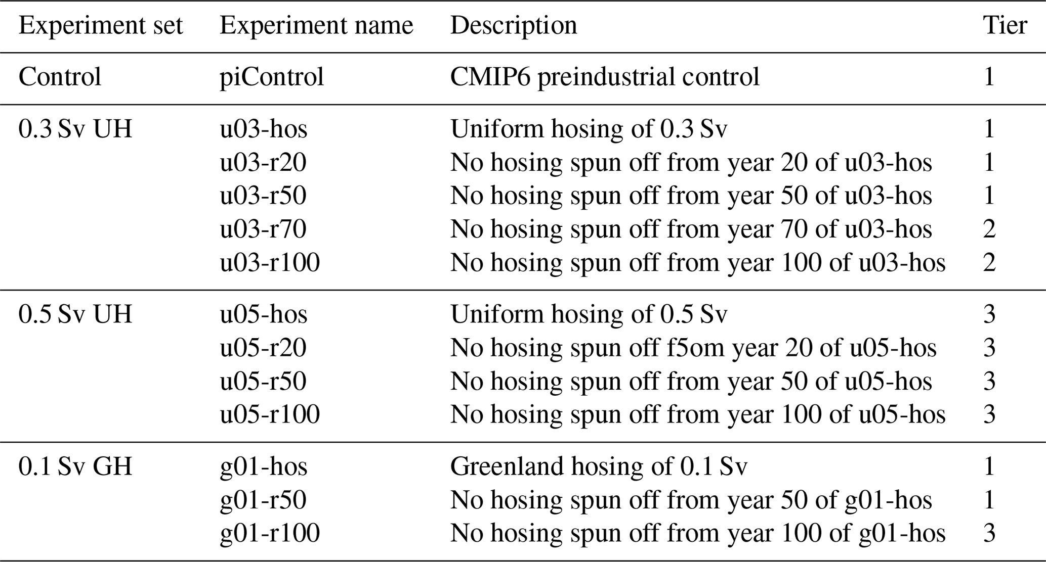
Experiments here are based on the preindustrial control experiments (where external forcings are fixed at 1850s conditions) which were conducted as part of the core CMIP6 experiments, described in Eyring et al. (2016). The experiments here use a preindustrial control state as an initial condition and are either hosing experiments (where an additional freshwater flux is applied to the surface ocean) or recovery experiments (with no hosing but starting from the hosing experiments). External forcings are otherwise the same as in the preindustrial control. A list of experiments is shown in Table 1.
2.1 Uniform-hosing experiments
To allow a clean comparison with Jackson and Wood (2018b), we use the same experimental protocol (uniform hosing from 50∘ N to the Bering Strait) and use a hosing strength of 0.3 Sv (1 Sv = 106 m3 s−1) for our uniform-hosing (UH) experiments. This rate of hosing allows us to compare the sensitivity of the different models and the processes and feedbacks involved, and it is strong enough that it is more likely that there is a significant response that can be compared.
Tier 1 (highest priority) experiments are a hosing experiment of 0.3 Sv (u03-hos, which should be continued for at least 50 years) and recovery experiments with no hosing spun off from years 20 and 50 of the hosing experiment (u03-r20, u03-r50). These recovery experiments should be run for 100 years, unless the AMOC immediately starts recovering, in which case 50 years is sufficient. Tier 2 is to continue the hosing experiment to 100 years with a recovery run after 100 years (u03-r100), although for the results presented here, one model instead did a recovery run after 70 years (u03-r70).
Tier 3 experiments are to repeat the UH experiment and recovery runs for a larger hosing rate of 0.5 Sv (u05-hos). This might be of interest if the AMOC recovers in all the previous experiments.
2.2 Greenland-hosing experiments
In addition to the UH experiments, we also propose a more realistic set of Greenland-hosing (GH) experiments, where the hosing is applied around Greenland using the method of Gerdes et al. (2006). For this set of experiments, a hosing of 0.1 Sv is used, which is considered to be a large estimate of potential freshwater input from melting glaciers in Greenland (Swingedouw et al., 2007).
Since the surface freshwater will be exported across 50∘ N and the Bering Strait in different ways due to the different distributions of hosing in the two sets of experiments, using the same magnitude of hosing would not allow for a clean comparison. Hence, we prefer to pick the rate of hosing most appropriate for each set of experiments.
Tier 1 experiments involve applying a hosing of 0.1 Sv over a region defined around Greenland (see below) for at least 50 years (g01-hos), as well as a recovery experiment with no hosing spun off from year 50 of the hosing experiment (g01-r50). The recovery experiment should again be run for 100 years, unless the AMOC immediately starts recovering, in which case 50 years is sufficient.
Tier 3 experiments are to continue the hosing experiment to 100 years, with a recovery experiment spun off after 100 years (g01-r100).
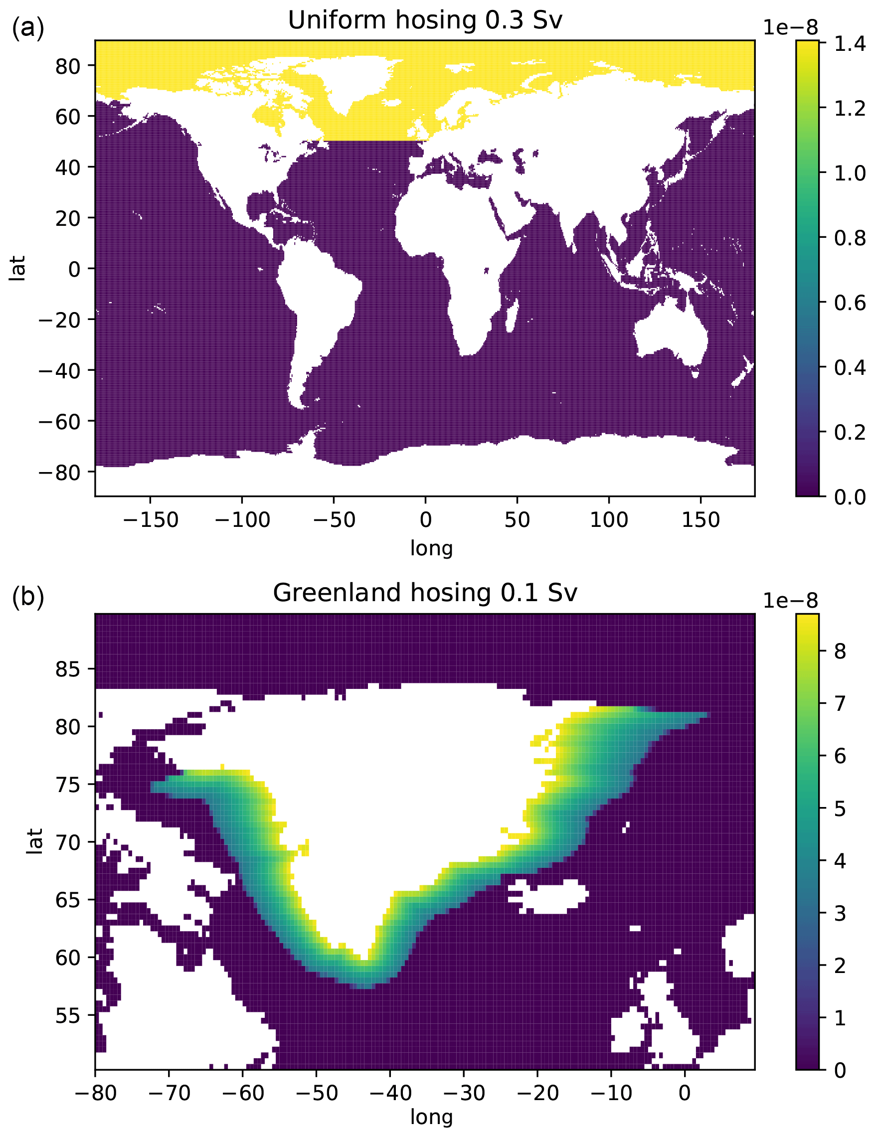
Figure 1Hosing fields: (a) shows the hosing field used for u03-hos, and (b) shows the hosing field used for g01-hos. Units are m s−1.
2.3 Hosing fields
2.3.1 Uniform-hosing field
To create the hosing field h for the UH experiments, we firstly define the region R1, which is the region north of 50∘ N in the Atlantic to the Bering Strait at 66∘ N (including the Arctic).
For a given hosing of H (in m3 s−1), a hosing field can then be created:
where dx and dy are the zonal and meridional grid spacings, and i and j are the zonal and meridional grid coordinates. Hence, . This hosing field is shown in the top panel of Fig. 1.
2.3.2 Greenland-hosing field
Following the protocol defined on http://www.clivar.org/clivar-panels/omdp/core-3 (last access: 29 March 2023) and in Gerdes et al. (2006), we define the region R2 as being around the coasts of Greenland from 76∘ N on the west side (Nares Strait) down to the tip of Greenland and up to 81∘ N on the east side (Fram Strait). See Fig. 3 of Gerdes et al. (2006). The hosing field is then given by
where r is the distance perpendicular to the coast, rmax=300 km, and α is given by
This hosing field is shown in the bottom panel of Fig. 1.
2.3.3 Applying hosing fields
In the past, most models have used rigid lids or linear free surfaces and have applied freshwater fluxes as virtual salinity fluxes (i.e. they do not add volume to the ocean); however, some models now use a nonlinear free surface, which means precipitation adds volume to the ocean. When applying the hosing flux h, we do not want to change the volume (which would cause difficulties when applying the compensation), so we apply it as a virtual salinity flux fs:
where S0 is the local salinity in the top model layer, and dz0 is the top-layer thickness (Roullet and Madec, 2000). Note the negative sign, since hosing reduces the salinity. Since h has units of m s−1, fs has units of PSU s−1 and is applied to the salinity budget calculation.
Note that, in the results shown below, the CESM2 model used a reference salinity rather than the local surface salinity.
2.3.4 Compensation
To stop the global salinity from drifting, we apply a volume compensation designed to conserve salt. Firstly, we calculate the total flux added,
and the total ocean volume,
Then the hosing correction applied is
This correction is calculated at each time step (since S0 varies) and is applied at all grid points in the ocean volume (including the hosing region). The implied salinity change of the correction at any grid point is much smaller than that of the hosing – for instance, in a model with a top-layer thickness of 1 m, the salinity change for the compensation is ∼ 0.001 % of that for the hosing.
2.4 Other experimental data
We also make use of other experiments conducted as part of CMIP6. The preindustrial control (piControl) experiments (documented in Eyring et al., 2016) are used as the initial conditions for hosing experiments and are used for comparing model mean states. References for data from the piControl experiments are Danabasoglu et al. (2019), Swart et al. (2019a), EC-Earth-Consortium (2019b), Ridley et al. (2018), Ridley et al. (2019c), Boucher et al. (2018b), Wieners et al. (2019a), and Jungclaus et al. (2019a). Where there is more than one ensemble member for a model, the r1i1p1f1 member is used, except in the CanESM5 model, where ensemble member r1i1p2f1 is used.
The abrupt 4 × CO2 experiments quadrupled the CO2 concentrations at the start of the experiment (branching out from the CMIP6 preindustrial controls) and are documented in Eyring et al. (2016). These experiments were conducted by all the models participating in this study (Swart et al., 2019b; EC-Earth-Consortium, 2019c; Boucher et al., 2018c; Ridley et al., 2019d, 2020; Jungclaus et al., 2019b; Wieners et al., 2019b; Danabasoglu, 2019b).
We also use the CMIP6 historical experiments (also documented in Eyring et al. (2016)) to compare AMOC strengths with observed values. For each model, an ensemble of historical experiments from 1850–2014 were run, with the ensembles having been generated by perturbations of the initial conditions. We calculate the AMOC strength and its uncertainty by using the mean and standard deviation across the available ensemble members. References for the data used are Danabasoglu (2019a), Swart et al. (2019c), EC-Earth-Consortium (2019a), Ridley et al. (2019a), Ridley et al. (2019b), Boucher et al. (2018a), Wieners et al. (2019c), and Jungclaus et al. (2019c).
3.1 Model description
The experimental protocol described in the previous section has been carried out by several GCMs which have previously participated in CMIP6. These are all fully coupled climate models. There are eight GCMs from six modelling centres, with two modelling centres (Met Office and Max Planck Institute, MPI) submitting two models with differing resolutions (Table 2). Most use the NEMO ocean model but with different atmosphere models; however, there are also GCMs based on the POP (CESM2) and MPIOM (MPI-ESM-LR and HR) ocean models. Most of the GCMs have a 1∘ horizontal ocean resolution, though HadGEM3-GC3-1MM has a higher resolution of . Although the two MPI models nominally have very different resolutions, the resolution in the subpolar North Atlantic is actually similar in both (Jungclaus et al., 2013).
Williams et al. (2018)Williams et al. (2018)Swart et al. (2019d)Döscher et al. (2022)Danabasoglu et al. (2020)Boucher et al. (2020)Mauritsen et al. (2019)Müller et al. (2018)Table 2Models used in this study. First column lists the models. Second column shows the AMOC strength in the historical experiments over the years 2005–2014, with the mean and twice the standard deviation of the ensemble values. Subsequent columns list the component atmosphere, ocean and sea ice models, the nominal ocean resolution number of vertical levels, and references. Those models which have demonstrated an AMOC hysteresis in this study are in bold.
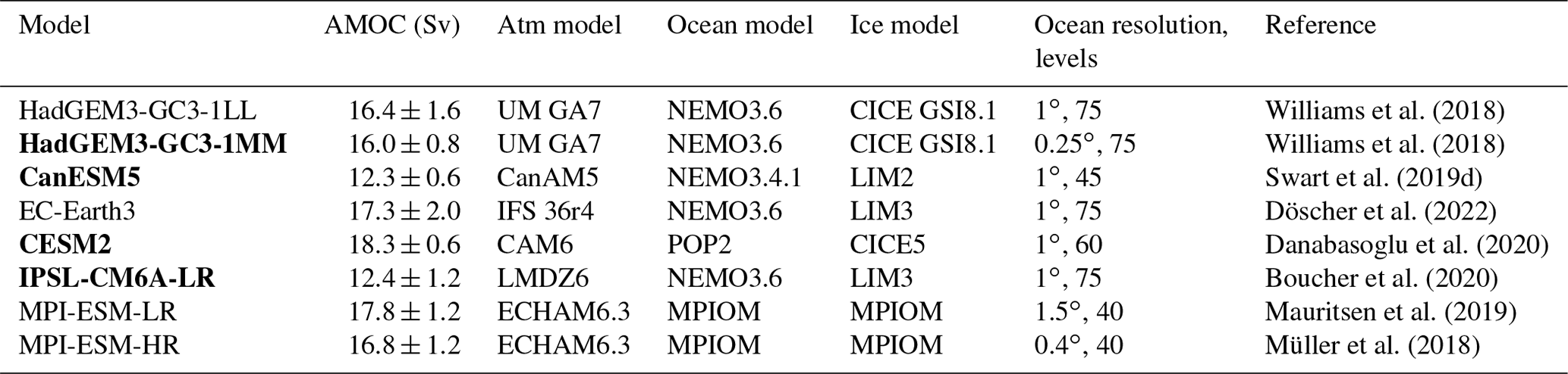
Table 3Parameterisations of mixing with typical values in m2 s−1. For mesoscale advection and diffusion the models use the formulations in Gent and McWilliams (1990, GM90) and Redi (1982, R82) or the formulation in Griffies (1998, G98). Those models with a submesoscale parameterisation use Fox-Kemper et al. (2011). For vertical diffusivity the models use the turbulent kinetic energy scheme described in Madec et al. (2012, TKE12) or in Madec et al. (2016, TKE16) or the schemes in Pacanowski and Philander (1981, PP) and Large et al. (1994, KPP). Those models which have demonstrated an AMOC hysteresis in this study are in bold.
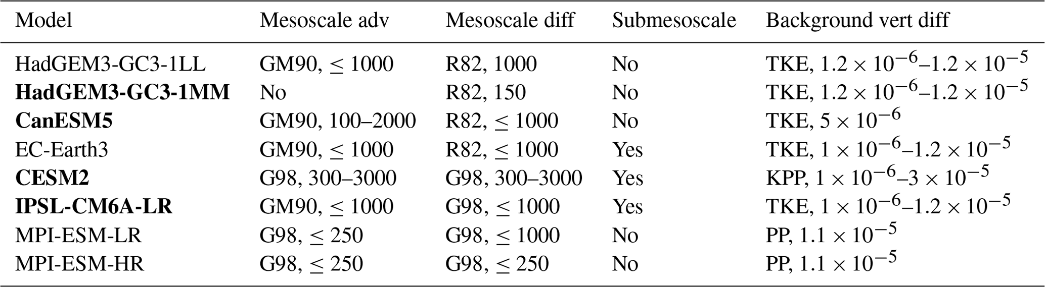
Since previous studies have shown that model representations of eddy mixing and diffusivity can have an impact on AMOC hysteresis, we include some of these details in Table 3. This includes details of mesoscale and submesoscale parameterisations and typical values, as well as parameterisations and typical values for background vertical diffusivity. It should be noted that models can have a much larger vertical diffusivity in the boundary layer and in certain regions as a result of the parameterisations of processes such as shear mixing, convection, double diffusion, and tidal mixing.
3.2 Diagnostics
We make use of the standard diagnostics used for CMIP6, as defined by Griffies et al. (2016). These include the following: the Atlantic meridional overturning circulation in depth coordinates, the barotropic stream function, sea surface temperature and salinity, and the March mean mixed-layer depth (the depth at which the buoyancy difference from the surface is 0.0003 m s−2). From the latter, we also use the mixed volume as an alternative metric for deep convection that takes account of the area of deep convection (Brodeau and Koenigk, 2016; Koenigk et al., 2021). This is calculated here as the volume of water above the mixed-layer depth and below 100 m.
We also use diagnostics of the overturning component of the Atlantic freshwater transport (Fov). This is calculated as , where is the zonal mean of the meridional velocity, is the zonal mean of the salinity, and S0 is a reference salinity (Rahmstorf, 1996; Hawkins et al., 2011; Weaver et al., 2012). This is calculated with monthly mean velocity and salinity fields, which ignores the impacts of the higher-frequency covariances of v and S; however, previous studies have found these to be small (Mecking et al., 2016; Jackson and Wood, 2018a). We use a reference salinity of 35 PSU, except in the case of CESM2, for which a reference salinity of 34.7 PSU is used, although the implied difference in transports from these different reference salinities is again very small (Mecking et al., 2017).
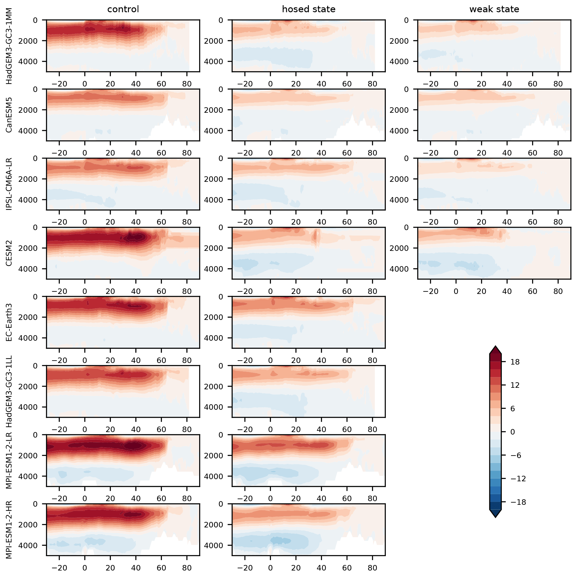
Figure 2Time mean stream functions (Sv). Each row shows AMOC stream functions from different models. The first column shows the control, the second column shows years 40–50 of u03-hos, and the third column shows years 50–100 of the recovery experiments where the AMOC stays weak. For HadGEM3-GC3-1MM and CESM2, this is experiment u03-r50; for IPSL-CM6A-LR, this is experiment u03-r100; and for CanESM5, this is experiment u03-r70.
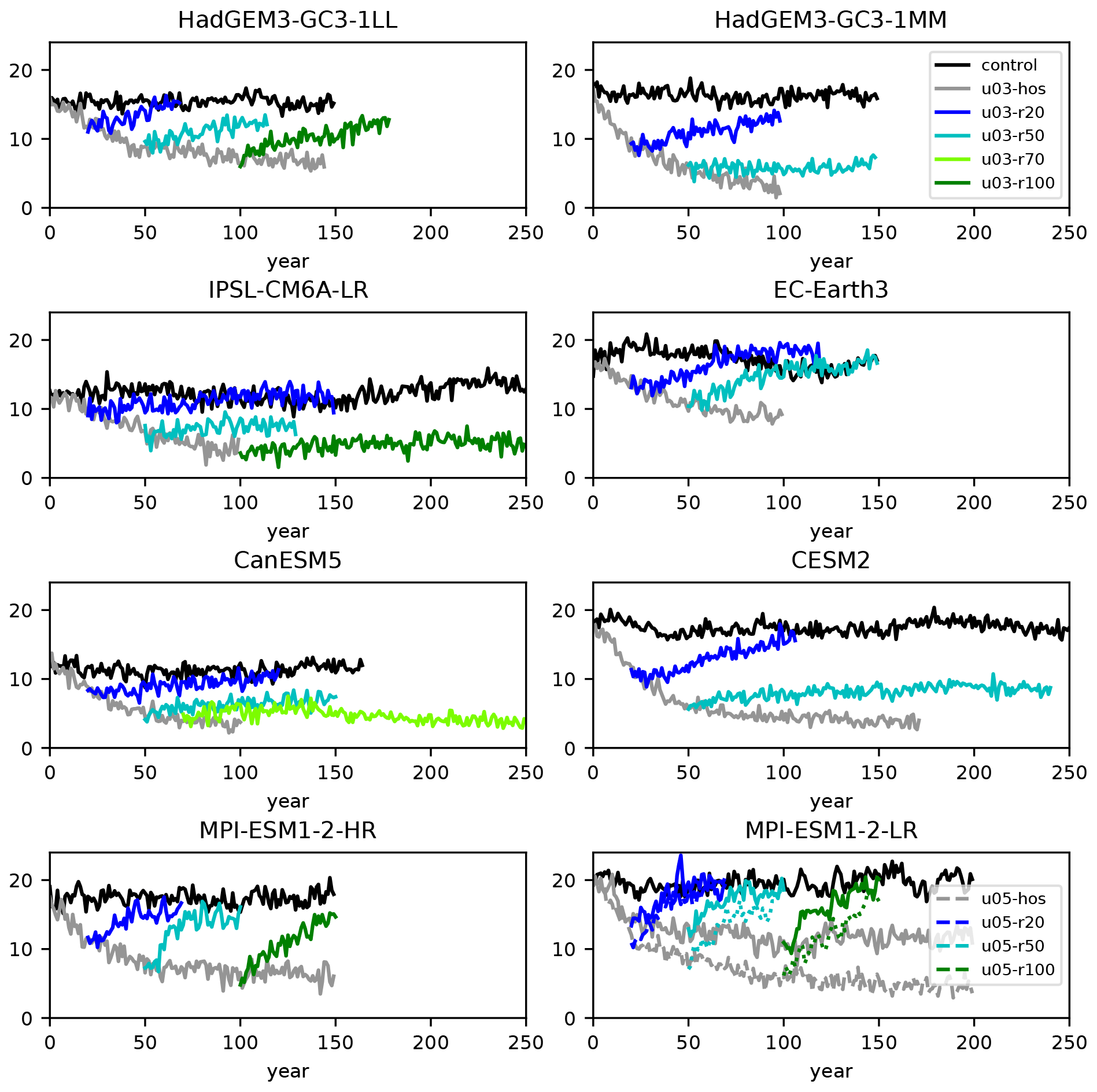
Figure 3AMOC strength (maximum in depth at 26.5∘ N) for UH experiments. Each panel shows experiments conducted with different models. Experiments are the control (black), u03-hos (grey), u03-r20 (blue), u03-r50 (cyan), u03-r70 (light green), and u03-r100 (green). MPI-ESM1-2-LR also shows the same experiment with a stronger hosing rate of 0.5 Sv (dashed lines).
4.1 AMOC response
4.1.1 Uniform-hosing experiments
The AMOC consists of an Atlantic overturning cell, with waters in the upper 1000 m travelling northwards on average, sinking in the North Atlantic, and returning southwards with a flow between 1000 and 3000 m (Fig. 2). Time series of the AMOC strength (defined as the maximum in depth at 26.5∘ N) for the set of UH experiments are shown in Fig. 3. During hosing, all models show an AMOC weakening, with a weakening and shallowing of the full AMOC cell (Fig. 2, middle column). In all models except CanESM5, a strengthening of the deep reversed Antarctic Bottom Water cell is also found.
Although many previous studies have found a relationship between AMOC control strength and AMOC weakening as a result of increased greenhouse gases (Gregory et al., 2005; Weaver et al., 2007; Winton et al., 2014; Weijer et al., 2020; Bellomo et al., 2021), this conclusion cannot be made for weakening as a result of hosing. The correlation between the weakening after 100 years of hosing and the control AMOC strength is not significant (−0.40, p=0.33), although the models with the strongest weakening are generally those with the strongest control strengths (Fig. 4a). The correlation with percentage AMOC weakening is also not significant (not shown). We also compare the AMOC weakening as a result of hosing in the u03-hos experiment with the AMOC weakening as a result of quadrupling CO2 in the 4 × CO2 experiment (Fig. 4c). Although there is a significant correlation between the AMOC weakening in the two experiments (0.73, p=0.04), this high correlation is caused by the two models, HadGEM3-GC3-1MM and CESM2, which have very large weakening in both experiments. It is possible that the processes responsible for the large AMOC sensitivity in these two models are the same in both scenarios. We note that the AMOC response to increased CO2 appears to be much stronger in some CMIP6 models in comparison to the previous CMIP5 models (Bellomo et al., 2021) and that the large weakening in HadGEM3-GC3-1MM and CESM2 is unusual for CMIP5 models but is found in other CMIP6 models. There is also a significant correlation (0.82, p=0.01) between the absolute strength reached after 100 years of hosing and the absolute strength reached after 150 years of quadrupled CO2 levels (Fig. 4d); we note that this correlation is not caused by outliers. In both experiments, the AMOC initially weakens quickly because of a large change in forcing, and then it weakens more gradually as the climate state adjusts. It may be that the feedbacks which oppose AMOC weakening are similar in the two different scenarios, as a result of which there is a statistical relationship between the equilibrium AMOC strengths. Data from Bellomo et al. (2021) show that the models in this study with weak AMOC states are unusually weak but within the range of other CMIP5 and CMIP6 models forced with an abrupt quadrupling of CO2. Given that the AMOC weakenings compared in Fig. 4c are defined as the differences between the final AMOC states (compared in Fig. 4d) and the control strengths, it is likely that a strong correlation in one would affect the other comparison. To conclude whether either of these conjectures (that the rate of weakening is similar between the two scenarios or that the final AMOC state is similar between the two scenarios) is true would require a greater number of model results or an improved understanding.
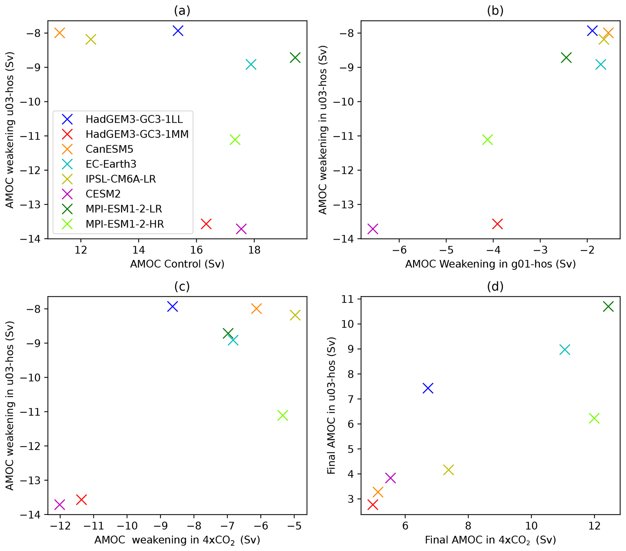
Figure 4Relationships of AMOC weakening. (a) Comparison of AMOC anomaly (year 90–100 mean in u03-hos) with the AMOC strength in the control. (b) Comparison of AMOC anomalies in u03-hos (year 90–100) and in g01-hos (year 40–50). (c) Comparison of AMOC anomalies (year 90–100) in u03-hos and (year 140–150) in the 4 × CO2 experiment. (d) As (c) but showing final AMOC strengths rather than anomalies. Colours indicate different models.
In the recovery experiments where the hosing is stopped after 20 years, the AMOC recovers towards its control state in all experiments. However, in some experiments, the AMOC demonstrates hysteresis by remaining in a weak state for at least 100 years after hosing stops. This occurs for HadGEM3-GC3-1MM and CESM2 after 50 years of hosing, for CanESM5 after 70 years of hosing, and for IPSL-CM6A-LR after 100 years of hosing. The stream functions of these weak states in the recovery experiments are shown in Fig. 2 (right column). There are a couple of experiments (IPSL-CM6A-LR and CanESM5 after 50 years of hosing) where the AMOC appears to stay in a weak state; however, a slight strengthening trend combined with short time series makes this conclusion uncertain. We cannot know whether the AMOC weak states are stable, since continuing the experiments for hundreds to thousands of years is prohibitive; however, they remain in the weak state for at least 100 years and so are quasi-stable weak states. It should be noted that these states differ from those in other studies that show reversed or completely collapsed states which are thought to be stable (Marotzke and Willebrand, 1991; Manabe and Stouffer, 1999; Gregory et al., 2003).
4.1.2 Greenland-hosing experiments
The second set of experiments performed examine the response of the AMOC to a more realistic freshwater input of 0.1 Sv around Greenland. Time series of AMOC strength are shown in Fig. 5. The AMOC reduction in all experiments is smaller than that in the previous experiments, likely because the rate of freshwater input is smaller. We note that, in additional experiments with MPI-ESM1-2-LR which use 0.3 Sv of hosing around Greenland, the AMOC weakening is slightly smaller than when applying the same amount uniformly.
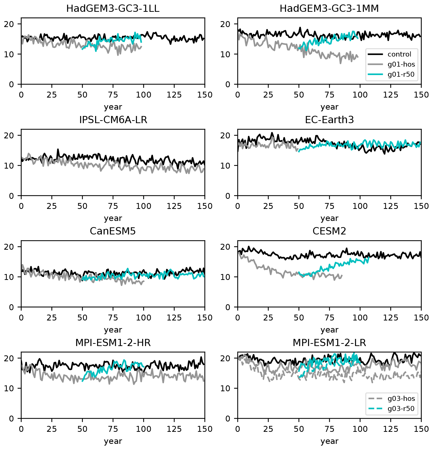
Figure 5AMOC strength (maximum in depth at 26.5∘ N) for GH experiments. Each panel shows experiments conducted with different models. Experiments are the control (black), g01-hos (grey), and g01-r50 (cyan). MPI-ESM1-2-LR also shows the same experiment with a stronger hosing rate of 0.3 Sv (dashed lines).
The location of the freshwater input around Greenland rather than spread uniformly over the subpolar Atlantic and Arctic could potentially be important, since the fresh anomalies can be easily exported from the subpolar North Atlantic by boundary currents and require resolved or parameterised eddies to mix the freshwater into the interior, where it impacts deep convection (Weijer et al., 2012; Swingedouw et al., 2022). Recent research has suggested that hosing around Greenland might be more effective in ocean models with a higher horizontal resolution, since the eddy mixing of the freshwater from boundary currents around Greenland into the interior might be stronger, resulting in a stronger inhibition of deep convection (Swingedouw et al., 2022). Although HadGEM3-GC3-1MM (which has the highest horizontal ocean resolution) has a strong AMOC weakening, there is a stronger AMOC weakening in CESM2, which has a lower resolution (Table 2).
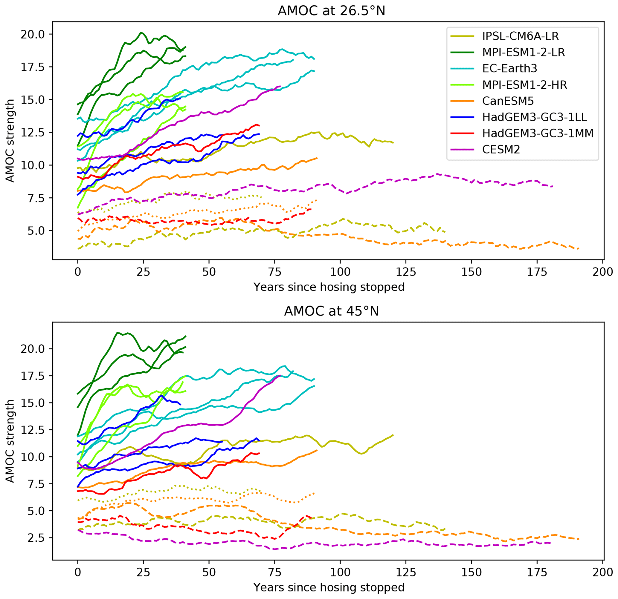
Figure 6AMOC time series in recovery experiments plotted as 10-year running means. All recovery experiments in the set have experienced UH of 0.3 Sv, with plotted time series starting from the time hosing stops. Colours show the model, with solid lines indicating experiments where the AMOC recovers, dashed lines indicating experiments where the AMOC stays in a weak state, and dotted lines indicating experiments where the AMOC response is uncertain. The top panel shows the AMOC measured at 26.5∘ N, and the bottom panel shows the AMOC at 45∘ N (maximum in depth).
A comparison of the AMOC weakening from both UH and GH experiments shows that those models with a stronger weakening as a result of one hosing scenario have a stronger weakening as a result of the other hosing scenario (Fig. 4b). Although the correlation is significant (0.90, p<0.01), there is a large difference in AMOC weakening in the g01-hos experiment in CESM2 and HadGEM3-GC3-1MM despite similar weakening in the u03-hos experiment. This suggests that the geographical distribution of hosing might impact different models differently.
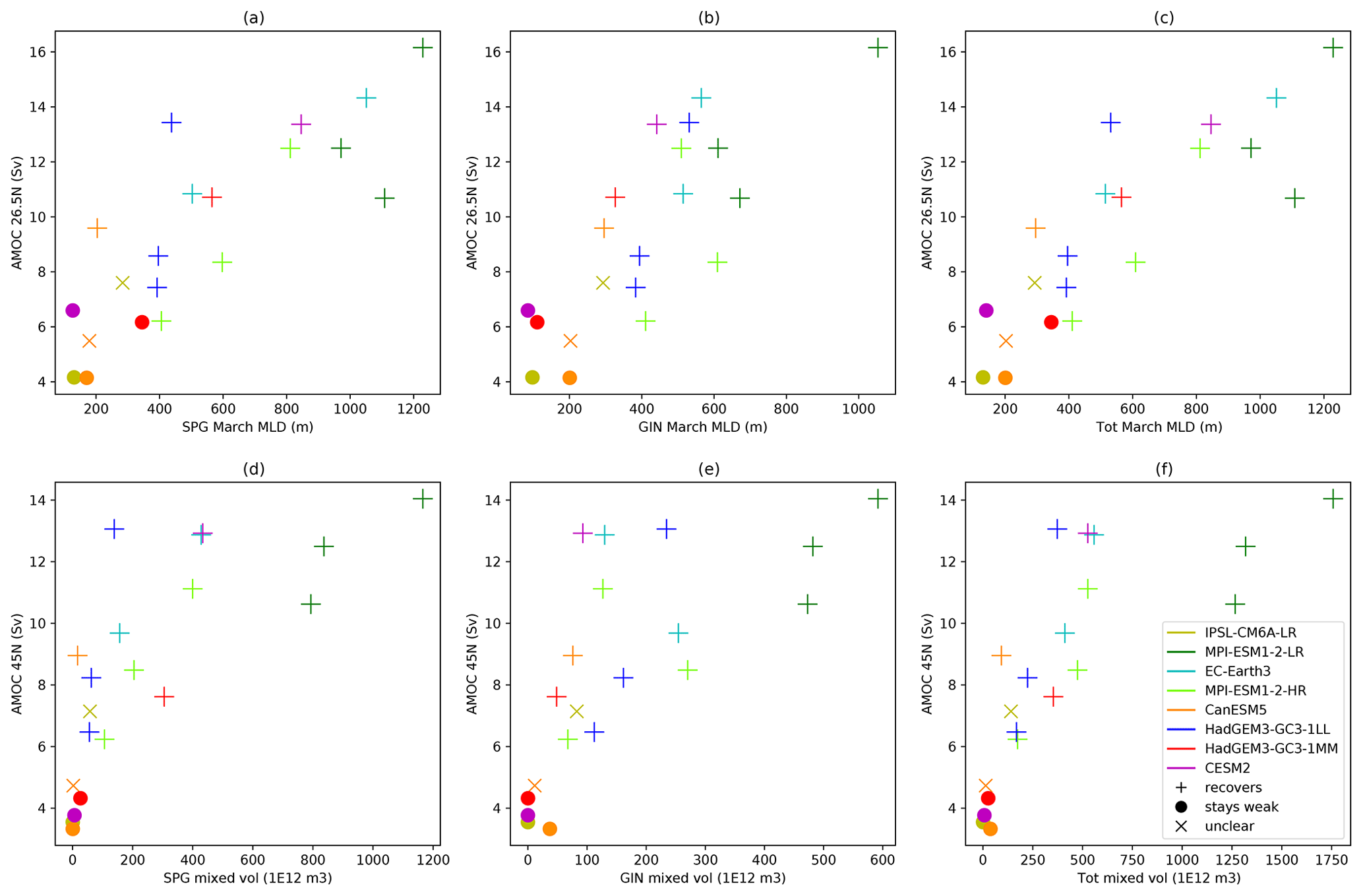
Figure 7Scatter plots of decadal means from the decade before hosing stops. Top panels: AMOC at 26.5∘ N against maximum mean March MLD over (a) the subpolar gyre (80∘ W–20∘ E, 50–65∘ N), (b) the GIN seas (50∘W–40∘ E, 65–80∘ N), and (c) the whole region (80∘ W–40∘ E, 50–80∘ N). (d)–(f) As (a)–(c) but for the AMOC at 45∘ N against the mixed volume (defined as the volume above the mixed-layer depth and below 100 m).
4.2 Exploration of the AMOC threshold
The experiments where the AMOC does not recover are the experiments where the AMOC reaches the weakest values (see Figs. 6 and 7). Although there is a clear separation at 26.5∘ N between the experiments where the AMOC recovers and where it does not when considering the first decade after hosing stops (Fig. 6), there is some overlap when considering the AMOC strength in the decade before the hosing stops (Fig. 7). Decadal means are used here to limit the impact of internal variability. There is a clearer separation when considering the AMOC at 45∘ N, with those experiments where the AMOC weakens to less than 5 Sv not showing a recovery (although for CanESM5, after 50 years of hosing, the results are uncertain). We note that, in the previous ensemble of HadGEM3-GC2 (a forerunner of HadGEM3-GC3-1MM) experiments, a threshold of 8 Sv (for AMOC at 26.5∘ N) was found (Jackson and Wood, 2018b). The clear separation seen between the experiments where the AMOC recovers and those where it does not is not found if we instead use AMOC anomalies or fractional changes rather than absolute values. Although the absolute values that the AMOC reaches during hosing appear to determine whether the AMOC subsequently recovers or remains in a weak state, it should be noted that, in experiments with HadGEM3-GC2 where the AMOC is weakened to 4 Sv by increasing CO2, the AMOC subsequently recovers when CO2 increases are reversed (not shown). Hence, it is likely that the weak AMOC state is indicative of other changes to the climate during hosing which sustain the weak state but also that these changes differ when the weakening is a result of increased CO2.
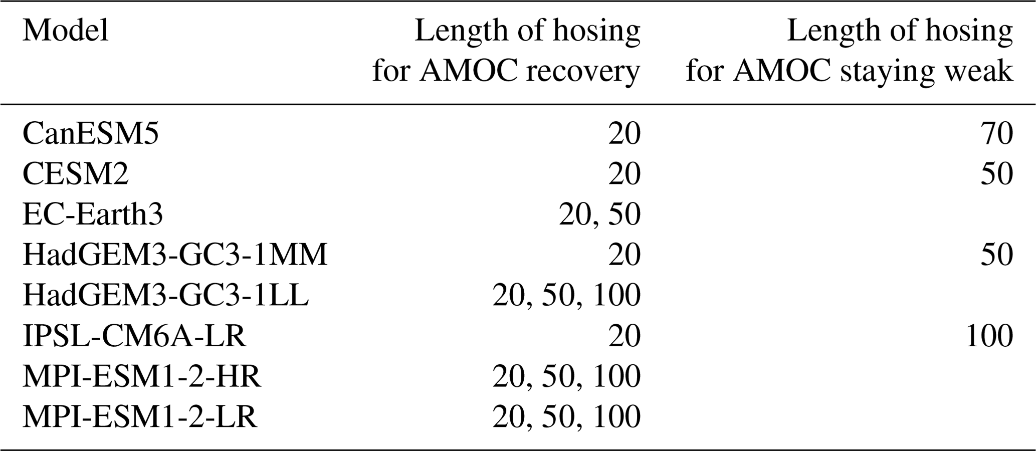
Table 4Length of hosing, which determines whether the AMOC stays weak or recovers after 0.3 Sv UH. States where the AMOC subsequently recovers when hosing stops (𝕊R) are listed in the middle column, and those states where the AMOC stays weak (𝕊W) are listed in the right column.
Those experiments where the AMOC does not recover also tend to have the weakest March mixed-layer depths (MLD) and the smallest March mixed volume (measured as the volume of water between the MLD and 100 m), both of which are measures of deep convection (Fig. 7). In particular, the MLD in the Greenland–Irminger–Norwegian (GIN) seas appears to be indicative of whether the AMOC will subsequently recover when hosing stops.
If we consider all the states that initialise the recovery experiments (taken as decadal means before the hosing stops), we can group these into states from which the AMOC subsequently recovers when hosing stops (named 𝕊R) and those states from which the AMOC stays weak (named 𝕊W). These states are characterised by the model and the number of years of hosing (using the UH 0.3 Sv hosing scenario) and are shown in Table 4. Examination of these states reveals differences in the sea surface temperatures (SST) and salinities (SSS) between these two groups. The decadal mean SST and SSS of all the states in 𝕊R and 𝕊W are shown in the top and middle panels of Fig. 8. These are calculated as decadal means of each group for the decade before hosing stops. Those states where the AMOC does not recover are, on average, colder and fresher than those states where the AMOC does recover. However, if SST or SSS were to be used to indicate which states had an AMOC which would recover or not, then all the states in 𝕊W would have to be colder or fresher than all the states in 𝕊R. To assess this we calculate for each grid point the coldest SST (or freshest SSS) from the states in 𝕊R and subtract the warmest SST (or saltiest SSS) from the states in 𝕊W. These metrics are plotted in the bottom panels of Fig. 8 and show that, in the Northeast Atlantic and the eastern Greenland–Irminger–Norwegian (GIN) seas, all states where the AMOC subsequently recovers are warmer and saltier (and denser – not shown) than all the states where the AMOC stays weak. In the states the AMOC recovers from, there is also generally less winter sea ice in the Northeast Atlantic (see contours, top panels of Fig. 8). States with denser surface waters and less winter sea ice would be more susceptible to the initiation of deep convection, which is consistent with the AMOC recovery.
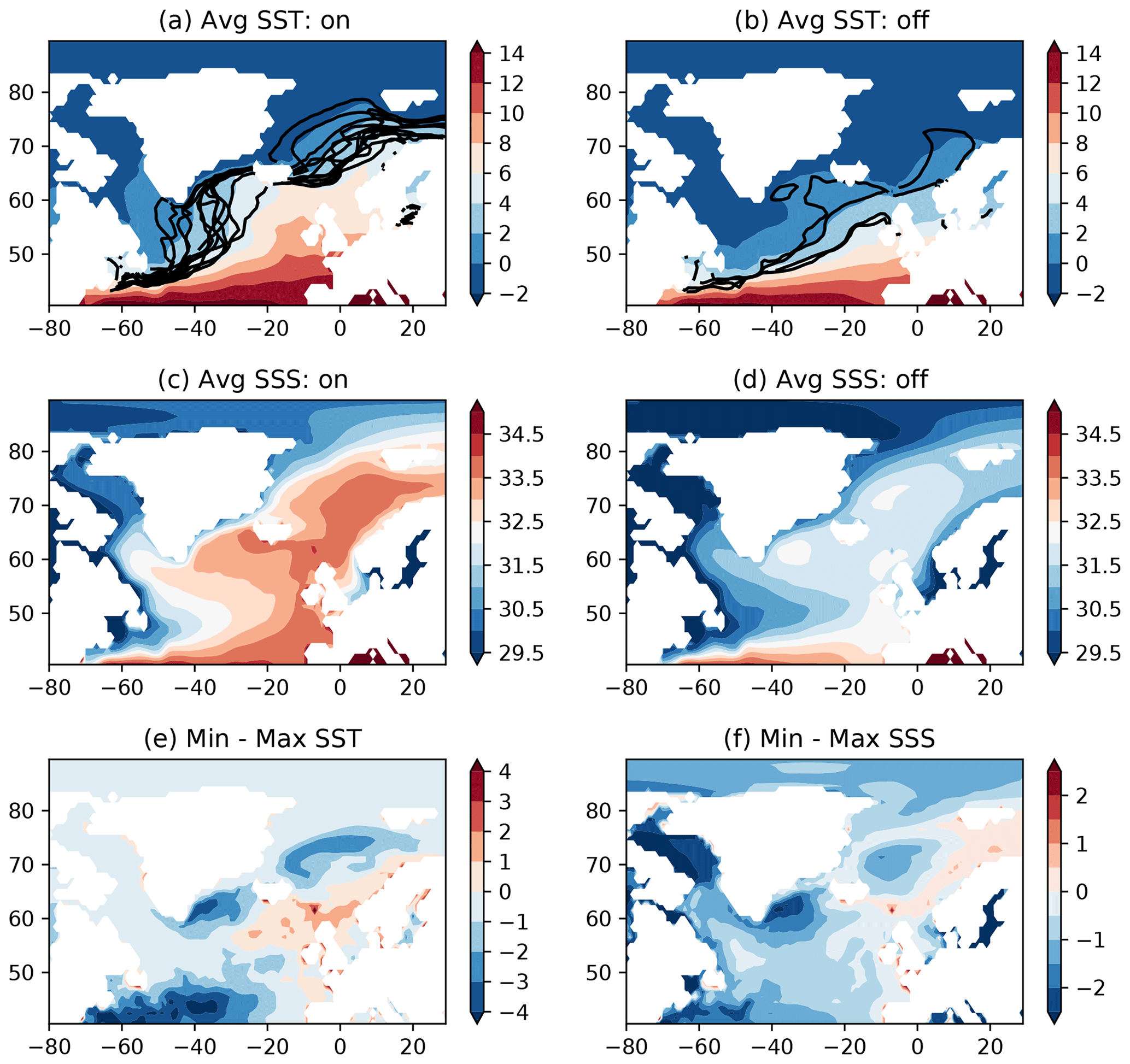
Figure 8Top panels show the mean SST (∘C) of (a) all the states in 𝕊R and (b) in 𝕊W (see Table 4). Black lines show winter sea ice extent (where concentration >20 %) from these states; (c) and (d) are as (a) and (b) but for SSS (PSU). Panel (e) shows the minimum SST of states in 𝕊R minus the maximum SST (∘C) of states in 𝕊W. Positive values suggest that all states in 𝕊R are warmer than all states in 𝕊W. Panel (f) shows the equivalent to panel (e) but for SSS (PSU).
4.3 Are there intrinsic model differences affecting the AMOC threshold?
One fundamental question is why the AMOC recovers after hosing in some models but not in others. We note that we find AMOC hysteresis in half the CMIP6 models tested (Table 4) and that this is not dependent on the ocean model used or the horizontal ocean resolution (Table 2). Since several studies have shown that increased vertical diffusivity can make the AMOC more stable (Schmittner and Weaver, 2001; Prange et al., 2003; Sijp and England, 2006), we examine the parameterisations and values of background vertical diffusivity in Table 3. There is no clear relationship between the models showing AMOC hysteresis; however, we note that GCMs have other parameterisations which enhance the vertical diffusivity near the surface and in particular locations (i.e. convection) – these enhanced diffusivities are not captured by the background values. Studies have also shown that increased mesoscale eddy advection and horizontal or isopycnal diffusion can also stabilise the AMOC (Hofmann and Rahmstorf, 2009; Dijkstra, 2007; Sijp and England, 2009; Sijp et al., 2006); however, Table 3 also shows no obvious relationship of the typical values or parameterisation schemes of mesoscale advection or diffusion with those models where the AMOC shows hysteresis.
Previous studies have suggested that the freshwater transport by the AMOC (Fov) in the South Atlantic is important for AMOC stability; if the AMOC exports freshwater, then weakening the AMOC would result in less freshwater being exported and hence a freshening and further weakening of the AMOC (Rahmstorf, 1996; Hawkins et al., 2011; Drijfhout et al., 2011). Mecking et al. (2016) argued that the greater export of freshwater in their model at 30∘ N was responsible for the AMOC not recovering after hosing and suggested that increased horizontal ocean resolution in their model increased Fov in the North Atlantic subtropics and strengthened this feedback. However, in the experiments in this study, it can be seen that there are models with a lower horizontal resolution (1∘ as opposed to 0.25∘) where the AMOC also does not recover, so this is not a feature of higher-resolution ocean models only. We also do not find any systematic difference in the control values of Fov at any latitude between those models where the AMOC recovers and those where it does not (Fig. 9), suggesting that this advective feedback does not determine which models show hysteresis.
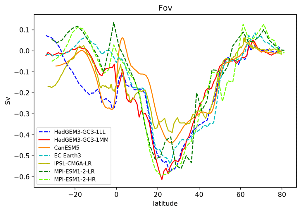
Figure 9Values of Fov (the freshwater transport by the AMOC in the Atlantic; Sv) by latitude for the control experiments. Different colours indicate different models, and solid (dashed) lines indicate those models which have (do not have) experiments where the AMOC stays weak after hosing stops.
Jackson et al. (2020) found that the AMOC response to increased greenhouse gases was sensitive to the amount of present-day water mass transformation (WMT) and mixed layer depth (MLD) in the west subpolar North Atlantic in a set of climate models. Here, comparisons of March MLD in the control experiments reveal no systematic difference between the models where the AMOC recovers and those where it remains weak (Fig. 10). Also, a comparison of WMT in some of the models considered here (Jackson and Petit, 2022) shows no systematic differences between models, with CanESM5 having little WMT in the Labrador and Iceland–Irminger seas and HadGEM3-GC3-1MM having strong WMT compared to other models. Likewise, there is no systematic difference between the two sets of models in terms of control AMOC strength (Fig. 3) or control SST, SSS, or ice extent (not shown).
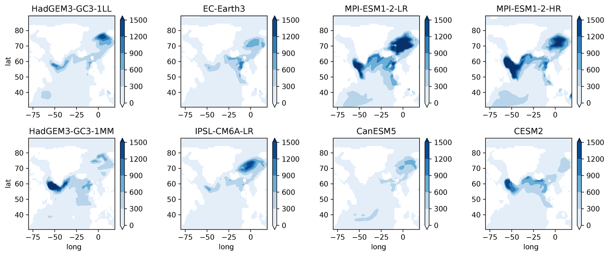
Figure 10Time mean March mixed-layer depth (m) in the control experiments. Models in the upper panels are those where the AMOC always recovers during subsequent recovery experiments, and models in the bottom panels are those where the AMOC stays in a weak state in at least one experiment.
Another model bias that might affect the AMOC response to hosing is the boundary between the subpolar and subtropical gyres. Swingedouw et al. (2013) proposed that, in models where the boundary is more zonal, freshwater that is added to the subpolar gyre is more easily exported to the subtropical gyre via the Canary Current in the eastern subtropical Atlantic. Inspection of the barotropic stream function for the models in this study (Fig. 11) reveals no systematic differences in the strengths of the subpolar or subtropical gyres or in the gradient of the intergyre boundary between the two sets of models in their control experiments. This might be due to the fact that uniform hosing has been used here, while Swingedouw et al. (2013) were analysing freshwater input around Greenland and the way it spread in the North Atlantic.

Figure 11Time mean barotropic stream function (Sv) in the control experiments. Models in the upper panels are those where the AMOC always recovers during subsequent recovery experiments, and models in the bottom panels are those where the AMOC stays in a weak state in at least one experiment. Black lines show the intergyre boundary between the subtropical and subpolar gyres over 15–45∘ W, with the gradient of the boundary listed in the panel titles (degrees latitude per degrees longitude).
Given that whether the AMOC recovers after hosing is dependent on the strength it reaches during hosing, the AMOC recovery could be dependent on both the AMOC strength in the control and its sensitivity to hosing (the amount of weakening it experiences). We note that IPSL-CM6A-LR and CanESM5 start from a state with a weak AMOC (11–12 Sv) and experience a small weakening of 5–6 Sv, whereas HadGEM3-GC3-1MM and CESM2 have a relatively strong AMOC in the control (16–18 Sv) and experience a large weakening (10–11 Sv). Present-day observations of the AMOC (Frajka-Williams et al., 2021) suggest a value of 16.8 Sv over the period 2005–2014. The strength of the AMOC in these models over this period is shown in Table 2. While the observational value lies within model uncertainty for most models, CanESM5 and IPSL-CM6A-LR have very weak AMOC strengths. Hence, of those models with a reasonable AMOC strength, only those with a strong AMOC weakening as a result of hosing reach a state where the AMOC does not recover.
We have presented the experimental protocol for the NAHosMIP project, which aims to understand the sensitivity of the AMOC to additional freshwater in the North Atlantic. We show that about half the CMIP6 models which run this protocol find states where the AMOC does not recover after hosing of 0.3 Sv. The difference in model behaviour cannot be explained by the ocean model resolution or type, by details of subgrid-scale parameterisations, or by aspects of the mean climate state such as the strength of the salinity advection feedback, the location or depth of deep convection, or the position of the intergyre boundary.
Instead, the AMOC behaviour appears to be related to the state the model reaches after hosing finishes; specifically, those experiments where the AMOC has reached the weakest states, where March mixed-layer depths are the shallowest, and where the eastern subpolar gyre and Nordic seas are the coldest and freshest with the greatest sea ice extent are those where the AMOC subsequently does not recover. An important question for further analysis is why different models reach different states during hosing.
Given that AMOC strength after hosing is a good indicator of AMOC recovery, it may be possible to relate AMOC recovery to the combination of AMOC control strength, sensitivity of the AMOC to freshwater forcing, and the duration of the freshwater input.
These results are all from experiments which apply an unrealistically large, idealised freshwater input and do not include warming from increasing greenhouse gases. So, although they are useful for understanding the model sensitivity, they should not be regarded as future scenarios. Results are also shown from an additional set of experiments where a large (but not unrealistic) freshwater flux is applied around Greenland to simulate freshwater from melting ice sheets. These results show AMOC weakening which varies a lot across models, with some models showing no weakening and others showing a weakening of several Sv in 50 years. While the AMOC shows no hysteresis from this less-idealised forcing, a sustained weakening would still have large impacts on climate.
Future studies will examine the mechanisms involved in the AMOC recovery to improve our understanding of the important feedbacks involved, as well as to examine the impacts of a sustained AMOC weakening. We also hope to use this protocol for future experiments with higher-resolution climate models, which improve the resolution of eddies and boundary currents in the subpolar North Atlantic. Understanding how the models' responses to freshwater forcing evolve in the presence of warming is also a future research direction.
Code and data used to do the analysis (including the annual mean AMOC stream function for all models) and code to plot figures in this paper are available from https://doi.org/10.5281/zenodo.7643437 (Jackson et al., 2022a). Other data from preindustrial control experiments are available via the Earth System Grid Federation (ESGF) servers, with information on obtaining data available from https://pcmdi.llnl.gov/CMIP6/Guide/dataUsers.html (last access: 5 May 2022). Code for creating hosing files and compensation and sample files are available from https://doi.org/10.5281/zenodo.7225014 (Jackson et al., 2022b).
LCJ led the paper, did the analysis, and wrote the paper. All the authors conducted the experiments, provided the diagnostics, and edited the paper.
The contact author has declared that none of the authors has any competing interests.
Publisher’s note: Copernicus Publications remains neutral with regard to jurisdictional claims in published maps and institutional affiliations.
Laura Claire Jackson was supported by the Met Office Hadley Centre Climate Programme funded by BEIS. Katinka Bellomo has received funding from the European Union’s Horizon 2020 research and innovation programme under the Marie Skłodowska-Curie Actions (grant no. 101026907 (CliMOC)). Aixue Hu was supported by the Regional and Global Model Analysis (RGMA) component of the Earth and Environmental System Modeling Program of the US Department of Energy's Office of Biological & Environmental Research (BER) via the National Science Foundation (grant no. IA 1844590). The EC-Earth3 simulations shown in this work were carried out at ECMWF under the special projects SPITBELL and SPITMEC2. This material is based upon work supported by the National Center for Atmospheric Research (NCAR), which is a major facility sponsored by the US National Science Foundation under Cooperative Agreement no. 1852977. This project is TiPES contribution no. 166, and this project has received funding from the European Unions Horizon 2020 research and innovation programme under grant agreement no. 820970.
This research has been supported by the Department for Business, Energy and Industrial Strategy, UK Government (Met Office Hadley Centre Climate Programme), the H2020 Marie Skłodowska-Curie Actions (grant no. 101026907), the Biological and Environmental Research (grant no. NSF IA 1844590), the European Centre for Medium-Range Weather Forecasts (grant nos. SPITBELL and SPITMEC2), the National Center for Atmospheric Research (grant no. 1852977), and the Horizon 2020 (grant no. 820970).
This paper was edited by Qiang Wang and reviewed by Wilbert Weijer and one anonymous referee.
Bakker, P., Schmittner, A., Lenaerts, J. T. M., Abe-Ouchi, A., Bi, D., van den Broeke, M. R., Chan, W. L., Hu, A., Beadling, R. L., Marsland, S. J., Mernild, S. H., Saenko, O. A., Swingedouw, D., Sullivan, A., and Yin, J.: Fate of the Atlantic Meridional Overturning Circulation: Strong decline under continued warming and Greenland melting, Geophys. Res. Lett., 43, 12252–12260, https://doi.org/10.1002/2016gl070457, 2016. a
Bellomo, K., Angeloni, M., Corti, S., and von Hardenberg, J.: Future climate change shaped by inter-model differences in Atlantic meridional overturning circulation response, Nat. Commun., 12, 3659, https://doi.org/10.1038/s41467-021-24015-w, 2021. a, b, c
Boucher, O., Denvil, S., Levavasseur, G., Cozic, A., Caubel, A., Foujols, M.-A., Meurdesoif, Y., Cadule, P., Devilliers, M., Ghattas, J., Lebas, N., Lurton, T., Mellul, L., Musat, I., Mignot, J., and Cheruy, F.: IPSL IPSL-CM6A-LR model output prepared for CMIP6 CMIP historical, WCRP [data set], https://doi.org/10.22033/ESGF/CMIP6.5195, 2018a. a
Boucher, O., Denvil, S., Levavasseur, G., Cozic, A., Caubel, A., Foujols, M.-A., Meurdesoif, Y., Cadule, P., Devilliers, M., Ghattas, J., Lebas, N., Lurton, T., Mellul, L., Musat, I., Mignot, J., and Cheruy, F.: IPSL IPSL-CM6A-LR model output prepared for CMIP6 CMIP piControl, WCRP [data set], https://doi.org/10.22033/ESGF/CMIP6.5251, 2018b. a
Boucher, O., Denvil, S., Levavasseur, G., Cozic, A., Caubel, A., Foujols, M.-A., Meurdesoif, Y., Cadule, P., Devilliers, M., Ghattas, J., Lebas, N., Lurton, T., Mellul, L., Musat, I., Mignot, J., and Cheruy, F.: IPSL IPSL-CM6A-LR model output prepared for CMIP6 CMIP abrupt-4xCO2, WCRP [data set], https://doi.org/10.22033/ESGF/CMIP6.5109, 2018c. a
Boucher, O., Servonnat, J., Albright, A. L., Aumont, O., Balkanski, Y., Bastrikov, V., Bekki, S., Bonnet, R., Bony, S., Bopp, L., Braconnot, P., Brockmann, P., Cadule, P., Caubel, A., Cheruy, F., Codron, F., Cozic, A., Cugnet, D., D'Andrea, F., Davini, P., de Lavergne, C., Denvil, S., Deshayes, J., Devilliers, M., Ducharne, A., Dufresne, J.-L., Dupont, E., Éthé, C., Fairhead, L., Falletti, L., Flavoni, S., Foujols, M.-A., Gardoll, S., Gastineau, G., Ghattas, J., Grandpeix, J.-Y., Guenet, B., Guez, Lionel, E., Guilyardi, E., Guimberteau, M., Hauglustaine, D., Hourdin, F., Idelkadi, A., Joussaume, S., Kageyama, M., Khodri, M., Krinner, G., Lebas, N., Levavasseur, G., Lévy, C., Li, L., Lott, F., Lurton, T., Luyssaert, S., Madec, G., Madeleine, J.-B., Maignan, F., Marchand, M., Marti, O., Mellul, L., Meurdesoif, Y., Mignot, J., Musat, I., Ottlé, C., Peylin, P., Planton, Y., Polcher, J., Rio, C., Rochetin, N., Rousset, C., Sepulchre, P., Sima, A., Swingedouw, D., Thiéblemont, R., Traore, A. K., Vancoppenolle, M., Vial, J., Vialard, J., Viovy, N., and Vuichard, N.: Presentation and Evaluation of the IPSL-CM6A-LR Climate Model, J. Adv. Model. Earth Sy., 12, e2019MS002010, https://doi.org/10.1029/2019MS002010, 2020. a
Brodeau, L. and Koenigk, T.: Extinction of the northern oceanic deep convection in an ensemble of climate model simulations of the 20th and 21st centuries, Clim. Dynam., 46, 2863–2882, https://doi.org/10.1007/s00382-015-2736-5, 2016. a
Clement, A. C. and Peterson, L. C.: Mechanisms of abrupt climate change of the last glacial period, Rev. Geophys., 46, RG4002, https://doi.org/10.1029/2006rg000204, 2008. a
Danabasoglu, G.: NCAR CESM2 model output prepared for CMIP6 CMIP historical, WCRP [data set], https://doi.org/10.22033/ESGF/CMIP6.7627, 2019a. a
Danabasoglu, G.: NCAR CESM2 model output prepared for CMIP6 CMIP abrupt-4xCO2, WCRP [data set], https://doi.org/10.22033/ESGF/CMIP6.7519, 2019b. a
Danabasoglu, G., Lawrence, D., Lindsay, K., Lipscomb, W., and Strand, G.: NCAR CESM2 model output prepared for CMIP6 CMIP piControl, WCRP [data set], https://doi.org/10.22033/ESGF/CMIP6.7733, 2019. a
Danabasoglu, G., Lamarque, J.-F., Bacmeister, J., Bailey, D. A., DuVivier, A. K., Edwards, J., Emmons, L. K., Fasullo, J., Garcia, R., Gettelman, A., Hannay, C., Holland, M. M., Large, W. G., Lauritzen, P. H., Lawrence, D. M., Lenaerts, J. T. M., Lindsay, K., Lipscomb, W. H., Mills, M. J., Neale, R., Oleson, K. W., Otto-Bliesner, B., Phillips, A. S., Sacks, W., Tilmes, S., van Kampenhout, L., Vertenstein, M., Bertini, A., Dennis, J., Deser, C., Fischer, C., Fox-Kemper, B., Kay, J. E., Kinnison, D., Kushner, P. J., Larson, V. E., Long, M. C., Mickelson, S., Moore, J. K., Nienhouse, E., Polvani, L., Rasch, P. J., and Strand, W. G.: The Community Earth System Model Version 2 (CESM2), J. Adv. Model. Earth Sy., 12, e2019MS001916, https://doi.org/10.1029/2019MS001916, 2020. a
den Toom, M., Dijkstra, H. A., Weijer, W., Hecht, M. W., Maltrud, M. E., and van Sebille, E.: Response of a Strongly Eddying Global Ocean to North Atlantic Freshwater Perturbations, J. Phys. Oceanogr., 44, 464–481, https://doi.org/10.1175/jpo-d-12-0155.1, 2014. a
de Vries, P. and Weber, S. L.: The Atlantic freshwater budget as a diagnostic for the existence of a stable shut down of the Meridional Overturning Circulation, Geophys. Res. Lett, 32, L09606, https://doi.org/10.1029/2004GL021450, 2005. a
Dijkstra, H. A.: Characterization of the multiple equilibria regime in a global ocean model, Tellus A, 59, 695–705, https://doi.org/10.1111/j.1600-0870.2007.00267.x, 2007. a, b
Döscher, R., Acosta, M., Alessandri, A., Anthoni, P., Arsouze, T., Bergman, T., Bernardello, R., Boussetta, S., Caron, L.-P., Carver, G., Castrillo, M., Catalano, F., Cvijanovic, I., Davini, P., Dekker, E., Doblas-Reyes, F. J., Docquier, D., Echevarria, P., Fladrich, U., Fuentes-Franco, R., Gröger, M., v. Hardenberg, J., Hieronymus, J., Karami, M. P., Keskinen, J.-P., Koenigk, T., Makkonen, R., Massonnet, F., Ménégoz, M., Miller, P. A., Moreno-Chamarro, E., Nieradzik, L., van Noije, T., Nolan, P., O'Donnell, D., Ollinaho, P., van den Oord, G., Ortega, P., Prims, O. T., Ramos, A., Reerink, T., Rousset, C., Ruprich-Robert, Y., Le Sager, P., Schmith, T., Schrödner, R., Serva, F., Sicardi, V., Sloth Madsen, M., Smith, B., Tian, T., Tourigny, E., Uotila, P., Vancoppenolle, M., Wang, S., Wårlind, D., Willén, U., Wyser, K., Yang, S., Yepes-Arbós, X., and Zhang, Q.: The EC-Earth3 Earth system model for the Coupled Model Intercomparison Project 6, Geosci. Model Dev., 15, 2973–3020, https://doi.org/10.5194/gmd-15-2973-2022, 2022. a
Drijfhout, S. S., Weber, S. L., and van der Swaluw, E.: The stability of the MOC as diagnosed from model projections for pre-industrial, present and future climates, Clim. Dynam., 37, 1575–1586, https://doi.org/10.1007/s00382-010-0930-z, 2011. a, b, c
EC-Earth-Consortium: EC-Earth-Consortium EC-Earth3 model output prepared for CMIP6 CMIP historical, WCRP [data set], https://doi.org/10.22033/ESGF/CMIP6.4700, 2019a. a
EC-Earth-Consortium: EC-Earth-Consortium EC-Earth3 model output prepared for CMIP6 CMIP piControl, WCRP [data set], https://doi.org/10.22033/ESGF/CMIP6.4842, 2019b. a
EC-Earth-Consortium: EC-Earth-Consortium EC-Earth3 model output prepared for CMIP6 CMIP abrupt-4xCO2, WCRP [data set], https://doi.org/10.22033/ESGF/CMIP6.4518, 2019c. a
Eyring, V., Bony, S., Meehl, G. A., Senior, C. A., Stevens, B., Stouffer, R. J., and Taylor, K. E.: Overview of the Coupled Model Intercomparison Project Phase 6 (CMIP6) experimental design and organization, Geosci. Model Dev., 9, 1937–1958, https://doi.org/10.5194/gmd-9-1937-2016, 2016. a, b, c, d
Fox-Kemper, B., Danabasoglu, G., Ferrari, R., Griffies, S., Hallberg, R., Holland, M., Maltrud, M., Peacock, S., and Samuels, B.: Parameterization of mixed layer eddies. III: Implementation and impact in global ocean climate simulations, Ocean Model., 39, 61–78, https://doi.org/10.1016/j.ocemod.2010.09.002, 2011. a
Frajka-Williams, E., Moat, B., Smeed, D., Rayner, D., Johns, W., Baringer, M., Volkov, D., and Collins, J.: Atlantic meridional overturning circulation observed by the RAPID-MOCHA-WBTS (RAPID-Meridional Overturning Circulation and Heatflux Array-Western Boundary Time Series) array at 26N from 2004 to 2020 (v2020.1), National Oceanography Centre [data set], https://doi.org/10.5285/cc1e34b3-3385-662b-e053-6c86abc03444, 2021. a
Gent, P. R. and McWilliams, J. C.: Isopycnal mixing in ocean circulation models, J. Phys. Oceanogr, 20, 150–155, 1990. a
Gerdes, R., Hurlin, W., and Griffies, S. M.: Sensitivity of a global ocean model to increased run-off from Greenland, Ocean Model., 12, 416–435, https://doi.org/10.1016/j.ocemod.2005.08.003, 2006. a, b, c
Gregory, J. M., Saenko, O. A., and Weaver, A. J.: The role of the Atlantic freshwater balance in the hysteresis of the meridional overturning circulation, Clim. Dynam., 21, 707–717, https://doi.org/10.1007/s00382-003-0359-8, 2003. a
Gregory, J. M., Dixon, K. W., Stouffer, R. J., Weaver, A. J., Driesschaert, E., Eby, M., Fichefet, T., Hasumi, H., Hu, A., Jungclaus, J. H., Kamenkovich, I. V., Levermann, A., Montoya, M., Murakami, S., Nawrath, S., Oka, A., Sokolov, A. P., and Thorpe, R. B.: A model intercomparison of changes in the Atlantic thermohaline circulation in response to increasing atmospheric CO2 concentration., Geophys. Res. Lett., 32, L12703, https://doi.org/10.1029/2005GL023209, 2005. a
Griffies, S. M.: The Gent-McWilliams Skew Flux, J. Phys. Oceanogr., 28, 831–841, https://doi.org/10.1175/1520-0485(1998)028<0831:TGMSF>2.0.CO;2, 1998. a
Griffies, S. M., Danabasoglu, G., Durack, P. J., Adcroft, A. J., Balaji, V., Böning, C. W., Chassignet, E. P., Curchitser, E., Deshayes, J., Drange, H., Fox-Kemper, B., Gleckler, P. J., Gregory, J. M., Haak, H., Hallberg, R. W., Heimbach, P., Hewitt, H. T., Holland, D. M., Ilyina, T., Jungclaus, J. H., Komuro, Y., Krasting, J. P., Large, W. G., Marsland, S. J., Masina, S., McDougall, T. J., Nurser, A. J. G., Orr, J. C., Pirani, A., Qiao, F., Stouffer, R. J., Taylor, K. E., Treguier, A. M., Tsujino, H., Uotila, P., Valdivieso, M., Wang, Q., Winton, M., and Yeager, S. G.: OMIP contribution to CMIP6: experimental and diagnostic protocol for the physical component of the Ocean Model Intercomparison Project, Geosci. Model Dev., 9, 3231–3296, https://doi.org/10.5194/gmd-9-3231-2016, 2016. a
Hawkins, E., Smith, R. S., Allison, L. C., Gregory, J. M., Woollings, T. J., Pohlmann, H., and de Cuevas, B.: Bistability of the Atlantic overturning circulation in a global climate model and links to ocean freshwater transport, Geophys. Res. Lett., 38, L10605, https://doi.org/10.1029/2011GL047208, 2011. a, b, c, d
Hofmann, M. and Rahmstorf, S.: On the stability of the Atlantic meridional overturning circulation, P. Natl. Acad. Sci. USA, 106, 20584–20589, https://doi.org/10.1073/pnas.0909146106, 2009. a, b, c
Hu, A., Meehl, G. A., Han, W., and Yin, J.: Transient response of the MOC and climate to potential melting of the Greenland Ice Sheet in the 21st century, Geophys. Res. Lett., 36, L10707, https://doi.org/10.1029/2009GL037998, 2009. a
Hu, A., Meehl, G. A., Han, W., Timmermann, A., Otto-Bliesner, B., Liu, Z., Washington, W. M., Large, W., Abe-Ouchi, A., Kimoto, M., Lambeck, K., and Wu, B.: Role of the Bering Strait on the hysteresis of the ocean conveyor belt circulation and glacial climate stability, P. Natl. Acad. Sci. USA, 109, 6417–6422, https://doi.org/10.1073/pnas.1116014109, 2012. a
Jackson, L. C.: Shutdown and recovery of the AMOC in a coupled global climate model: The role of the advective feedback, Geophys. Res. Lett., 40, 1182–1188, https://doi.org/10.1002/grl.50289, 2013. a, b, c
Jackson, L. C. and Petit, T.: North Atlantic overturning and water mass transformation in CMIP6 models, Clim. Dynam., https://doi.org/10.1007/s00382-022-06448-1, 2022. a
Jackson, L. C. and Wood, R. A.: Timescales of AMOC decline in response to fresh water forcing, Clim. Dynam., 51, 1333, https://doi.org/10.1007/s00382-017-3957-6, 2018a. a
Jackson, L. C. and Wood, R. A.: Hysteresis and resilience of the AMOC in an eddy2̆010permitting GCM, Geophys. Res. Lett., 45, 8547–8556, https://doi.org/10.1029/2018GL078104, 2018b. a, b, c, d, e
Jackson, L. C., Kahana, R., Graham, T., Ringer, M. A., Woollings, T., Mecking, J. V., and Wood, R. A.: Global and European climate impacts of a slowdown of the AMOC in a high resolution GCM, Clim. Dynam., 45, 3299–3316, https://doi.org/10.1007/s00382-015-2540-2, 2015. a
Jackson, L. C., Roberts, M. J., Hewitt, H. T., Iovino, D., Koenigk, T., Meccia, V. L., Roberts, C. D., Ruprich-Robert, Y., and Wood, R. A.: Impact of ocean resolution and mean state on the rate of AMOC weakening, Clim. Dynam., 55, 1711–1732, https://doi.org/10.1007/s00382-020-05345-9, 2020. a, b
Jackson, L., Alastue de Asenjo, E., Bellomo, K., Danabasoglu, G., Hu, A., Jungclaus, J., Lee, W., Meccia, V., Saenko, O., Shao, A., and Swingedouw, D.: NAHosMIP data (Version published), Zenodo [code and data set], https://doi.org/10.5281/zenodo.7643437, 2022a. a
Jackson, L., Alastue de Asenjo, E., Bellomo, K., Danabasoglu, G., Hu, A., Jungclaus, J., Lee, W., Meccia, V., Saenko, O., Shao, A., and Swingedouw, D.: NAHosMIP experimental protocol (Version published), Zenodo [code], https://doi.org/10.5281/zenodo.7225014, 2022b. a
Jungclaus, J., Bittner, M., Wieners, K.-H., Wachsmann, F., Schupfner, M., Legutke, S., Giorgetta, M., Reick, C., Gayler, V., Haak, H., de Vrese, P., Raddatz, T., Esch, M., Mauritsen, T., von Storch, J.-S., Behrens, J., Brovkin, V., Claussen, M., Crueger, T., Fast, I., Fiedler, S., Hagemann, S., Hohenegger, C., Jahns, T., Kloster, S., Kinne, S., Lasslop, G., Kornblueh, L., Marotzke, J., Matei, D., Meraner, K., Mikolajewicz, U., Modali, K., Müller, W., Nabel, J., Notz, D., Peters-von Gehlen, K., Pincus, R., Pohlmann, H., Pongratz, J., Rast, S., Schmidt, H., Schnur, R., Schulzweida, U., Six, K., Stevens, B., Voigt, A., and Roeckner, E.: MPI-M MPI-ESM1.2-HR model output prepared for CMIP6 CMIP piControl, WCRP [data set], https://doi.org/10.22033/ESGF/CMIP6.6674, 2019a. a
Jungclaus, J., Bittner, M., Wieners, K.-H., Wachsmann, F., Schupfner, M., Legutke, S., Giorgetta, M., Reick, C., Gayler, V., Haak, H., de Vrese, P., Raddatz, T., Esch, M., Mauritsen, T., von Storch, J.-S., Behrens, J., Brovkin, V., Claussen, M., Crueger, T., Fast, I., Fiedler, S., Hagemann, S., Hohenegger, C., Jahns, T., Kloster, S., Kinne, S., Lasslop, G., Kornblueh, L., Marotzke, J., Matei, D., Meraner, K., Mikolajewicz, U., Modali, K., Müller, W., Nabel, J., Notz, D., Peters-von Gehlen, K., Pincus, R., Pohlmann, H., Pongratz, J., Rast, S., Schmidt, H., Schnur, R., Schulzweida, U., Six, K., Stevens, B., Voigt, A., and Roeckner, E.: MPI-M MPI-ESM1.2-HR model output prepared for CMIP6 CMIP abrupt-4xCO2, WCRP [data set], https://doi.org/10.22033/ESGF/CMIP6.6458, 2019b. a
Jungclaus, J., Bittner, M., Wieners, K.-H., Wachsmann, F., Schupfner, M., Legutke, S., Giorgetta, M., Reick, C., Gayler, V., Haak, H., de Vrese, P., Raddatz, T., Esch, M., Mauritsen, T., von Storch, J.-S., Behrens, J., Brovkin, V., Claussen, M., Crueger, T., Fast, I., Fiedler, S., Hagemann, S., Hohenegger, C., Jahns, T., Kloster, S., Kinne, S., Lasslop, G., Kornblueh, L., Marotzke, J., Matei, D., Meraner, K., Mikolajewicz, U., Modali, K., Müller, W., Nabel, J., Notz, D., Peters-von Gehlen, K., Pincus, R., Pohlmann, H., Pongratz, J., Rast, S., Schmidt, H., Schnur, R., Schulzweida, U., Six, K., Stevens, B., Voigt, A., and Roeckner, E.: MPI-M MPI-ESM1.2-HR model output prepared for CMIP6 CMIP historical, WCRP [data set], https://doi.org/10.22033/ESGF/CMIP6.6594, 2019c. a
Jungclaus, J. H., Haak, H., Esch, M., Roeckner, E., and Marotzke, J.: Will Greenland melting halt the thermohaline circulation?, Geophys. Res. Lett., 33, L17708, https://doi.org/10.1029/2006GL026815, 2006. a
Jungclaus, J. H., Fischer, N., Haak, H., Lohmann, K., Marotzke, J., Matei, D., Mikolajewicz, U., Notz, D., and von Storch, J. S.: Characteristics of the ocean simulations in MPIOM, the ocean component of the MPI-Earth system model, J. Adv. Model. Earth Syst, 5, 422–446, https://doi.org/10.1002/jame.20023, 2013. a
Koenigk, T., Fuentes-Franco, R., Meccia, V. L., Gutjahr, O., Jackson, L. C., New, A. L., Ortega, P., Roberts, C. D., Roberts, M. J., Arsouze, T., Iovino, D., Moine, M.-P., and Sein, D. V.: Deep mixed ocean volume in the Labrador Sea in HighResMIP models, Clim. Dynam., 57, 1895–1918, https://doi.org/10.1007/s00382-021-05785-x, 2021. a
Large, W. G., McWilliams, J. C., and Doney, S. C.: Oceanic vertical mixing: A review and a model with a nonlocal boundary layer parameterization, Rev. Geophys., 32, 363–403, https://doi.org/10.1029/94RG01872, 1994. a
Lenaerts, J. T. M., Le Bars, D., van Kampenhout, L., Vizcaino, M., Enderlin, E. M., and van den Broeke, M. R.: Representing Greenland ice sheet freshwater fluxes in climate models, Geophys. Res. Lett., 42, 6373–6381, 2015. a
Liu, W., Liu, Z., and Brady, E. C.: Why is the AMOC Monostable in Coupled General Circulation Models?, J. Climate, 27, 2427–2443, https://doi.org/10.1175/jcli-d-13-00264.1, 2013. a
Liu, W., Xie, S.-P., Liu, Z., and Zhu, J.: Overlooked possibility of a collapsed Atlantic Meridional Overturning Circulation in warming climate, Science Advances, 3, e1601666, https://doi.org/10.1126/sciadv.1601666, 2017. a
Madec, G., Benshila, R., Bricaud, C., Coward, A., Dobricic, S., Furner, R., and Oddo, P.: NEMO ocean engine, in: Notes du Pôle de modélisation de l'Institut Pierre-Simon Laplace (IPSL) (v3.4, Number 27), Zenodo, https://doi.org/10.5281/zenodo.1464817, 2012. a
Madec, G., Bourdallé-Badie, R., Bouttier, P., Bricaud, C., Bruciaferri, D., Calvert, D., Chanut, J., Clementi, E., Coward, A., Delrosso, D., Ethé, C., Flavoni, S., Graham, T., Harle, J., Iovino, D., Lea, D., Lévy, C., Lovato, T., Martin, N., Masson, S., Mocavero, S., Paul, J., Rousset, C., Storkey, D., Storto, A., and Vancoppenolle, M.: NEMO ocean engine, in: Notes du Pôle de modélisation de l'Institut Pierre-Simon Laplace (IPSL) (v3.6, Number 27), Zenodo, https://doi.org/10.5281/zenodo.1472492, 2017. a
Manabe, B. S. and Stouffer, R. J.: Are two modes of thermohaline circulation stable?, Tellus A, 51, 400–411, https://doi.org/10.1034/j.1600-0870.1999.t01-3-00005.x, 1999. a
Marotzke, J. and Willebrand, J.: Multiple Equilibria of the Global Thermohaline Circulation, J. Phys. Oceanogr., 21, 1372–1385, https://doi.org/10.1175/1520-0485(1991)021<1372:meotgt>2.0.co;2, 1991. a
Mauritsen, T., Bader, J., Becker, T., Behrens, J., Bittner, M., Brokopf, R., Brovkin, V., Claussen, M., Crueger, T., Esch, M., Fast, I., Fiedler, S., Fläschner, D., Gayler, V., Giorgetta, M., Goll, D. S., Haak, H., Hagemann, S., Hedemann, C., Hohenegger, C., Ilyina, T., Jahns, T., Jimenéz-de-la Cuesta, D., Jungclaus, J., Kleinen, T., Kloster, S., Kracher, D., Kinne, S., Kleberg, D., Lasslop, G., Kornblueh, L., Marotzke, J., Matei, D., Meraner, K., Mikolajewicz, U., Modali, K., Möbis, B., Müller, W. A., Nabel, J. E. M. S., Nam, C. C. W., Notz, D., Nyawira, S.-S., Paulsen, H., Peters, K., Pincus, R., Pohlmann, H., Pongratz, J., Popp, M., Raddatz, T. J., Rast, S., Redler, R., Reick, C. H., Rohrschneider, T., Schemann, V., Schmidt, H., Schnur, R., Schulzweida, U., Six, K. D., Stein, L., Stemmler, I., Stevens, B., von Storch, J.-S., Tian, F., Voigt, A., Vrese, P., Wieners, K.-H., Wilkenskjeld, S., Winkler, A., and Roeckner, E.: Developments in the MPI-M Earth System Model version 1.2 (MPI-ESM1.2) and Its Response to Increasing CO2, J. Adv. Model. Earth Sy., 11, 998–1038, https://doi.org/10.1029/2018MS001400, 2019. a
McManus, J. F., Francois, R., Gherardi, J. M., Keigwin, L. D., and Brown-Leger, S.: Collapse and rapid resumption of Atlantic meridional circulation linked to deglacial climate changes, Nature, 428, 834–837, https://doi.org/10.1038/nature02494, 2004. a
Mecking, J. V., Drijfhout, S. S., Jackson, L. C., and Graham, T.: Stable AMOC off state in an eddy-permitting coupled climate model, Clim. Dynam., 47, 2455–2470, https://doi.org/10.1007/s00382-016-2975-0, 2016. a, b, c, d, e
Mecking, J. V., Drijfhout, S. S., Jackson, L. C., and Andrews, M. B.: The effect of model bias on Atlantic freshwater transport and implications for AMOC bi-stability, Tellus A, 69, 1299910, https://doi.org/10.1080/16000870.2017.1299910, 2017. a, b
Müller, W. A., Jungclaus, J. H., Mauritsen, T., Baehr, J., Bittner, M., Budich, R., Bunzel, F., Esch, M., Ghosh, R., Haak, H., Ilyina, T., Kleine, T., Kornblueh, L., Li, H., Modali, K., Notz, D., Pohlmann, H., Roeckner, E., Stemmler, I., Tian, F., and Marotzke, J.: A Higher-resolution Version of the Max Planck Institute Earth System Model (MPI-ESM1.2-HR), J. Adv. Model. Earth Sy., 10, 1383–1413, https://doi.org/10.1029/2017MS001217, 2018. a
Pacanowski, R. C. and Philander, S. G. H.: Parameterization of Vertical Mixing in Numerical Models of Tropical Oceans, J. Phys. Oceanogr., 11, 1443–1451, https://doi.org/10.1175/1520-0485(1981)011<1443:POVMIN>2.0.CO;2, 1981. a
Prange, M., Lohmann, G., and Paul, A.: Influence of Vertical Mixing on the Thermohaline Hysteresis: Analyses of an OGCM, J. Phys. Oceanogr., 33, 1707–1721, https://doi.org/10.1175/1520-0485(2003)033<1707:IOVMOT>2.0.CO;2, 2003. a, b
Rahmstorf, S.: On the freshwater forcing and transport of the Atlantic Thermohaline Circulation, Clim. Dynam., 12, 799–811, https://doi.org/10.1007/s003820050144, 1996. a, b, c, d
Rahmstorf, S.: Ocean circulation and climate during the past 120,000 years, Nature, 419, 207–214, https://doi.org/10.1038/nature01090, 2002. a
Rahmstorf, S., Crucifix, M., Ganopolski, A., Goosse, H., Kamenkovich, I., Knutti, R., Lohmann, G., Marsh, R., Mysak, L. A., Wang, Z., and and Weaver, A. J.: Thermohaline circulation hysteresis: A model intercomparison, Geophys. Res. Lett, 32, L23605, https://doi.org/10.1029/2005GL023655, 2005. a, b
Redi, M. H.: Oceanic Isopycnal Mixing by Coordinate Rotation, J. Phys. Oceanogr., 12, 1154–1158, https://doi.org/10.1175/1520-0485(1982)012<1154:OIMBCR>2.0.CO;2, 1982. a
Ridley, J., Menary, M., Kuhlbrodt, T., Andrews, M., and Andrews, T.: MOHC HadGEM3-GC31-LL model output prepared for CMIP6 CMIP piControl, WCRP [data set], https://doi.org/10.22033/ESGF/CMIP6.6294, 2018. a
Ridley, J., Menary, M., Kuhlbrodt, T., Andrews, M., and Andrews, T.: MOHC HadGEM3-GC31-LL model output prepared for CMIP6 CMIP historical, WCRP [data set], https://doi.org/10.22033/ESGF/CMIP6.6109, 2019a. a
Ridley, J., Menary, M., Kuhlbrodt, T., Andrews, M., and Andrews, T.: MOHC HadGEM3-GC31-MM model output prepared for CMIP6 CMIP historical, WCRP [data set], https://doi.org/10.22033/ESGF/CMIP6.6112, 2019b. a
Ridley, J., Menary, M., Kuhlbrodt, T., Andrews, M., and Andrews, T.: MOHC HadGEM3-GC31-MM model output prepared for CMIP6 CMIP piControl, WCRP [data set], https://doi.org/10.22033/ESGF/CMIP6.6297, 2019c. a
Ridley, J., Menary, M., Kuhlbrodt, T., Andrews, M., and Andrews, T.: MOHC HadGEM3-GC31-LL model output prepared for CMIP6 CMIP abrupt-4xCO2, WCRP [data set], https://doi.org/10.22033/ESGF/CMIP6.5839, 2019d. a
Ridley, J., Menary, M., Kuhlbrodt, T., Andrews, M., and Andrews, T.: MOHC HadGEM3-GC31-MM model output prepared for CMIP6 CMIP abrupt-4xCO2, WCRP [data set], https://doi.org/10.22033/ESGF/CMIP6.5842, 2020. a
Roullet, G. and Madec, G.: Salt conservation, free surface, and varying levels: A new formulation for ocean general circulation models, J. Geophys. Res.-Oceans, 105, 23927–23942, https://doi.org/10.1029/2000JC900089, 2000. a
Schmittner, A. and Weaver, A.: Dependence of multiple climate states on ocean mixing parameters, Geophys. Res. Lett., 28, 1027–1030, https://doi.org/10.1029/2000GL012410, 2001. a, b
Sijp, W. and England, M.: Sensitivity of the Atlantic Thermohaline Circulation and Its Stability to Basin-Scale Variations in Vertical Mixing, J. Climate, 19, 5467–5478, https://doi.org/10.1175/JCLI3909.1, 2006. a, b
Sijp, W. P. and England, M. H.: The Control of Polar Haloclines by Along-Isopycnal Diffusion in Climate Models, J. Climate, 22, 486–498, https://doi.org/10.1175/2008JCLI2513.1, 2009. a, b
Sijp, W. P., Bates, M., and England, M. H.: Can Isopycnal Mixing Control the Stability of the Thermohaline Circulation in Ocean Climate Models?, J. Climate, 19, 5637–5651, https://doi.org/10.1175/JCLI3890.1, 2006. a, b
Stommel, H.: Thermohaline convection with two stable regimes of flow, Tellus, 13, 224–230, 1961. a
Stouffer, R. J., Yin, J., Gregory, J. M., Dixon, K. W., Spelman, M. J., Hurlin, W., Weaver, A. J., Eby, M., Flato, G. M., Hasumi, H., Hu, A., Jungclaus, J. H., Kamenkovich, I. V., Levermann, A., Montoya, M., Murakami, S., Nawrath, S., Oka, A., Peltier, W. R., Robitaille, D. Y., Sokolov, A., Vettoretti, G., and Weber, S. L.: Investigating the Causes of the Response of the Thermohaline Circulation to Past and Future Climate Changes., J. Climate, 19, 1365–1387, https://doi.org/10.1175/JCLI3689.1, 2006. a
Swart, N. C., Cole, J. N., Kharin, V. V., Lazare, M., Scinocca, J. F., Gillett, N. P., Anstey, J., Arora, V., Christian, J. R., Jiao, Y., Lee, W. G., Majaess, F., Saenko, O. A., Seiler, C., Seinen, C., Shao, A., Solheim, L., von Salzen, K., Yang, D., Winter, B., and Sigmond, M.: CCCma CanESM5 model output prepared for CMIP6 CMIP piControl, WCRP [data set], https://doi.org/10.22033/ESGF/CMIP6.3673, 2019a. a
Swart, N. C., Cole, J. N., Kharin, V. V., Lazare, M., Scinocca, J. F., Gillett, N. P., Anstey, J., Arora, V., Christian, J. R., Jiao, Y., Lee, W. G., Majaess, F., Saenko, O. A., Seiler, C., Seinen, C., Shao, A., Solheim, L., von Salzen, K., Yang, D., Winter, B., and Sigmond, M.: CCCma CanESM5 model output prepared for CMIP6 CMIP abrupt-4xCO2, WCRP [data set], https://doi.org/10.22033/ESGF/CMIP6.3532, 2019b. a
Swart, N. C., Cole, J. N., Kharin, V. V., Lazare, M., Scinocca, J. F., Gillett, N. P., Anstey, J., Arora, V., Christian, J. R., Jiao, Y., Lee, W. G., Majaess, F., Saenko, O. A., Seiler, C., Seinen, C., Shao, A., Solheim, L., von Salzen, K., Yang, D., Winter, B., and Sigmond, M.: CCCma CanESM5 model output prepared for CMIP6 CMIP historical, WCRP [data set], https://doi.org/10.22033/ESGF/CMIP6.3610, 2019c. a
Swart, N. C., Cole, J. N. S., Kharin, V. V., Lazare, M., Scinocca, J. F., Gillett, N. P., Anstey, J., Arora, V., Christian, J. R., Hanna, S., Jiao, Y., Lee, W. G., Majaess, F., Saenko, O. A., Seiler, C., Seinen, C., Shao, A., Sigmond, M., Solheim, L., von Salzen, K., Yang, D., and Winter, B.: The Canadian Earth System Model version 5 (CanESM5.0.3), Geosci. Model Dev., 12, 4823–4873, https://doi.org/10.5194/gmd-12-4823-2019, 2019d. a
Swingedouw, D., Braconnot, P., Delecluse, P., Guilyardi, E., and Marti, O.: Quantifying the AMOC feedbacks during a 2 × CO2 stabilization experiment with land-ice melting, Clim. Dynam., 29, 521–534, https://doi.org/10.1007/s00382-007-0250-0, 2007. a
Swingedouw, D., Rodehacke, C., Behrens, E., Menary, M., Olsen, S., Gao, Y., Mikolajewicz, U., Mignot, J., and Biastoch, A.: Decadal fingerprints of freshwater discharge around Greenland in a multi-model ensemble, Clim. Dynam., 41, 695–720, https://doi.org/10.1007/s00382-012-1479-9, 2013. a, b
Swingedouw, D., Houssais, M.-N., Herbaut, C., Blaizot, A.-C., Devilliers, M., and Deshayes, J.: AMOC Recent and Future Trends: A Crucial Role for Oceanic Resolution and Greenland Melting?, Frontiers in Climate, 4, 838310, https://doi.org/10.3389/fclim.2022.838310, 2022. a, b, c
van den Berk, J. and Drijfhout, S.: A realistic freshwater forcing protocol for ocean-coupled climate models, Ocean Model., 81, 36–48, https://doi.org/10.1016/j.ocemod.2014.07.003, 2014. a
Weaver, A. J., Eby, M., Kienast, M., and Saenko, O. A.: Response of the Atlantic meridional overturning circulation to increasing atmospheric CO2: Sensitivity to mean climate state, Geophys. Res. Lett., 34, L05708, https://doi.org/10.1029/2006GL028756, 2007. a
Weaver, A. J., Sedládek, J., Eby, M., Alexander, K., Crespin, E., Fichefet, T., Philippon-Berthier, G., Joos, F., Kawamiya, M., Matsumoto, K., Steinacher, M., Tachiiri, K., Tokos, K., Yoshimori, M., and Zickfeld, K.: Stability of the Atlantic meridional overturning circulation: A model intercomparison, Geophys. Res. Lett., 39, L20709, https://doi.org/10.1029/2012GL053763, 2012. a
Weijer, W., Maltrud, M. E., Hecht, M. W., Dijkstra, H. A., and Kliphuis, M. A.: Response of the Atlantic Ocean circulation to Greenland Ice Sheet melting in a strongly-eddying ocean model, Geophys. Res. Lett., 39, L09606, https://doi.org/10.1029/2012gl051611, 2012. a, b
Weijer, W., Cheng, W., Drijfhout, S. S., Federov, A., Hu, A., Jackson, L. C., Liu, W., McDonagh, E. L., Mecking, J. V., and Zhang, J.: Stability of the Atlantic Meridional Overturning Circulation: A review and synthesis., J. Geophys. Res.-Oceans, 124, 5336–5375, https://doi.org/10.1029/2019JC015083, 2019. a, b
Weijer, W., Cheng, W., Garuba, O., Hu, A., and Nadiga, B.: CMIP6 Models Predict Significant 21st Century Decline of the Atlantic Meridional Overturning Circulation, Geophys. Res. Lett., 47, e2019GL086075, https://doi.org/10.1029/2019GL086075, 2020. a
Wieners, K.-H., Giorgetta, M., Jungclaus, J., Reick, C., Esch, M., Bittner, M., Legutke, S., Schupfner, M., Wachsmann, F., Gayler, V., Haak, H., de Vrese, P., Raddatz, T., Mauritsen, T., von Storch, J.-S., Behrens, J., Brovkin, V., Claussen, M., Crueger, T., Fast, I., Fiedler, S., Hagemann, S., Hohenegger, C., Jahns, T., Kloster, S., Kinne, S., Lasslop, G., Kornblueh, L., Marotzke, J., Matei, D., Meraner, K., Mikolajewicz, U., Modali, K., Müller, W., Nabel, J., Notz, D., Peters-von Gehlen, K., Pincus, R., Pohlmann, H., Pongratz, J., Rast, S., Schmidt, H., Schnur, R., Schulzweida, U., Six, K., Stevens, B., Voigt, A., and Roeckner, E.: MPI-M MPI-ESM1.2-LR model output prepared for CMIP6 CMIP piControl, WCRP [data set], https://doi.org/10.22033/ESGF/CMIP6.6675, 2019a. a
Wieners, K.-H., Giorgetta, M., Jungclaus, J., Reick, C., Esch, M., Bittner, M., Legutke, S., Schupfner, M., Wachsmann, F., Gayler, V., Haak, H., de Vrese, P., Raddatz, T., Mauritsen, T., von Storch, J.-S., Behrens, J., Brovkin, V., Claussen, M., Crueger, T., Fast, I., Fiedler, S., Hagemann, S., Hohenegger, C., Jahns, T., Kloster, S., Kinne, S., Lasslop, G., Kornblueh, L., Marotzke, J., Matei, D., Meraner, K., Mikolajewicz, U., Modali, K., Müller, W., Nabel, J., Notz, D., Peters-von Gehlen, K., Pincus, R., Pohlmann, H., Pongratz, J., Rast, S., Schmidt, H., Schnur, R., Schulzweida, U., Six, K., Stevens, B., Voigt, A., and Roeckner, E.: MPI-M MPI-ESM1.2-LR model output prepared for CMIP6 CMIP abrupt-4xCO2, WCRP [data set], https://doi.org/10.22033/ESGF/CMIP6.6459, 2019b. a
Wieners, K.-H., Giorgetta, M., Jungclaus, J., Reick, C., Esch, M., Bittner, M., Legutke, S., Schupfner, M., Wachsmann, F., Gayler, V., Haak, H., de Vrese, P., Raddatz, T., Mauritsen, T., von Storch, J.-S., Behrens, J., Brovkin, V., Claussen, M., Crueger, T., Fast, I., Fiedler, S., Hagemann, S., Hohenegger, C., Jahns, T., Kloster, S., Kinne, S., Lasslop, G., Kornblueh, L., Marotzke, J., Matei, D., Meraner, K., Mikolajewicz, U., Modali, K., Müller, W., Nabel, J., Notz, D., Peters-von Gehlen, K., Pincus, R., Pohlmann, H., Pongratz, J., Rast, S., Schmidt, H., Schnur, R., Schulzweida, U., Six, K., Stevens, B., Voigt, A., and Roeckner, E.: MPI-M MPI-ESM1.2-LR model output prepared for CMIP6 CMIP historical, WCRP [data set], https://doi.org/10.22033/ESGF/CMIP6.6595, 2019c. a
Williams, K. D., Copsey, D., Blockley, E. W., Bodas-Salcedo, A., Calvert, D., Comer, R., Davis, P., Graham, T., Hewitt, H. T., Hill, R., Hyder, P., Ineson, S., Johns, T. C., Keen, A. B., Lee, R. W., Megann, A., Milton, S. F., Rae, J. G. L., Roberts, M. J., Scaife, A. A., Schiemann, R., Storkey, D., Thorpe, L., Watterson, I. G., Walters, D. N., West, A., Wood, R. A., Woollings, T., and Xavier, P. K.: The Met Office Global Coupled Model 3.0 and 3.1 (GC3.0 and GC3.1) Configurations, J. Adv. Model. Earth Sy., 10, 357–380, https://doi.org/10.1002/2017ms001115, 2018. a, b
Winton, M., Anderson, W. G., Delworth, T. L., Griffies, S. M., Hurlin, W. J., and Rosati, A.: Has coarse ocean resolution biased simulations of transient climate sensitivity?, Geophys. Res. Lett., 41, 8522–8529, https://doi.org/10.1002/2014GL061523, 2014. a