A methodological framework for improving the performance of data-driven models: a case study for daily runoff prediction in the Maumee domain, USA

Geoscientific models are simplified representations of complex earth and environmental systems (EESs). Compared with physics-based numerical models, data-driven modeling has gained popularity due mainly to data proliferation in EESs and the ability to perform prediction without requiring explicit mathematical representation of complex biophysical processes. However, because of the black-box nature of data-driven models, their performance cannot be guaranteed. To address this issue, we developed a generalizable framework for improving the efficiency and effectiveness of model training and the reduction of model overfitting. This framework consists of two parts: hyperparameter selection based on Sobol global sensitivity analysis and hyperparameter tuning using a Bayesian optimization approach. We demonstrated the framework efficacy through a case study of daily edge-of-field (EOF) runoff predictions by a tree-based data-driven model using the extreme gradient boosting (XGBoost) algorithm in the Maumee domain, USA. This framework contributes towards improving the performance of a variety of data-driven models and can thus help promote their applications in EESs.

1 Introduction

Geoscientific models are simplified representations of complex earth and environmental systems (EESs), where predictive models can have a wide range of applications. For example, they can incorporate and advance the scientific knowledge of EESs and assess how EESs react to changing conditions (Fleming et al., 2021; Reichstein et al., 2019). Furthermore, evidence-based decisions and policies on EESs can be made by effectively evaluating their influences using these models (Fleming et al., 2021; Prinn, 2013), which would otherwise be impossible or too costly and time-consuming to implement in practice (Hu et al., 2015; Sohl and Claggett, 2013).

Two broad classes of models are often used to predict target environmental phenomena in EESs: physics-based numerical models, and data-driven machine learning models. Conventionally, the modeling of EESs relies heavily on physics-based models, developed based on the first principles of physics (Bergen et al., 2019), which require comprehensive understanding of the target EES and proper mathematical representations of all processes relevant to the target phenomena. As such, the long development time, insufficient representations of system components, and difficulties in access and use set barriers for the wide application of such models. On the contrary, despite the fact that data-driven models are data-intensive and not generalizable (Ford et al., 2022), they do not require an explicit mathematical formulation of all underlying complex processes to perform predictive analysis. Thus, the development of data-driven models is often less involved. Moreover, the proliferation of data further leads to the rise of data-driven modeling in EESs (Willard et al., 2020).

For data-driven modeling, model performance relies heavily on the capability of the underlying machine learning (ML) algorithms to retrieve information from data; this capability is controlled by the complexity of ML algorithms and their associated parameters, that is, hyperparameters (Yang and Shami, 2020; Hutter et al., 2015). When the underlying ML algorithm is too simple to learn complex patterns from data, we see large biases in the training phase (i.e., underfitting; Jabbar and Khan, 2015; Koehrsen, 2018). In contrast, model overfitting occurs when the ML algorithm is overcomplicated to capture all random noises in the training data; the resulting model performs very well in training but poorly on the test (i.e., variance error). As such, to improve model performance, we need to determine appropriate ML algorithms that can balance model bias and variance error (Koehrsen, 2018).

There are various rules of thumb to choose an appropriate ML algorithm for data-driven modeling. When the model is underfitting, we can choose more complex ML algorithms (e.g., from linear regression models to tree-based regression models). However, in practice it can be more challenging to reduce overfitting; model overfitting is often associated with a long training time and poor performance in test sets. Because of the black-box nature of data-driven models, only a handful of approaches is available to deal with overfitting. One such approach is random sampling with or without replacement (Gimenez-Nadal et al., 2019) in which data points are randomly selected for training and test. This approach attempts to ensure that the data samples are uniformly distributed: both the training and test sets have data points to represent the entire domain space. Combined with this approach, other approaches such as early stopping (Yao et al., 2007), cross-validation (Fushiki, 2011), and regularization techniques (Zhu et al., 2018) are used to address overfitting by tuning hyperparameters to balance model performance in training and test sets.

Hyperparameters affect model performance through ML algorithms during model training, although they are external parameters to data-driven models. However, not all hyperparameters have the same level of impact on model performance, as they affect different aspects of ML algorithms to retrieve data patterns. For example, some hyperparameters control the algorithm complexity, while some are used to reduce overfitting as mentioned above. By tuning these hyperparameters, we want to identify optimal hyperparameter values for the ML algorithm. We can then apply the optimized ML algorithm to maximize the model performance during training.

Tuning hyperparameters manually becomes unfeasible as the number of hyperparameters associated with the ML algorithm increases. Hyperparameter optimization algorithms are developed to automatically identify the optimal hyperparameters to maximize model performance by minimizing a predefined objective function (i.e., loss function) of a data-driven model. A variety of optimization approaches are available and categorized based on the mechanisms used to search the optimal hyperparameter values: (I) exhaustive search using grid or random search (Liashchynskyi and Liashchynskyi, 2019; Bergstra et al., 2011) and (II) surrogate models using sequential model-based optimization (SMBO) methods (Bergstra et al., 2011). The choice of tuning approaches is affected by several factors, such as the number of hyperparameters, different ranges of their values, and the complexity of ML algorithms. In general, compared to the category I approaches, the category II approaches are more suitable for data-driven models with complex ML algorithms (Bergstra et al., 2011).

Rather than tuning all hyperparameters, it is expected to be more efficient and effective if we only need to tune a subset of them to achieve similar or better model performance. Similarly to assessing the overall impact of model parameters on model prediction for physics-based models, we can use global sensitivity analysis approaches to identify critical hyperparameters for model performance based on sensitivity scores (Sobol, 2001); hyperparameters with high sensitivity scores are considered influential, while the rest with low sensitivity scores are considered to have no or negligible influence on model performance. Additionally, since fewer influential hyperparameters are involved in model training, less training time is required to achieve maximum model performance. Therefore, it is particularly useful if data-driven models need to be trained with streaming data for real-time predictions (Gomes et al., 2017).

With the proliferation of data in EESs, we expect to have more EES applications using data-driven models. In this study, we present a new framework for data-driven modeling that combines hyperparameter selection and tuning to minimize training time, reduce overfitting, and maximize overall model performance. As such, the fundamental contribution of our work is a framework which can (1) identify a subset of hyperparameters critical for model performance through hyperparameter selection using a variance-based sensitivity analysis approach, and (2) provide optimal values for the selected hyperparameters through an optimization-based hyperparameter tuning approach. As such, we can improve the overall efficiency and effectiveness of model training, leading to better model performance. In turn, this can further promote the use of data-driven models in EESs. The efficacy of the framework is evaluated using data-driven models developed to predict the magnitudes of daily surface runoff at a farm scale in the Maumee domain, USA.

2 Method

In this study, we developed a framework to improve the performance of data-driven models by reducing their training time and overfitting. The framework comprises two modules: hyperparameter selection (HS) and hyperparameter tuning (HT; Fig. 1). To use the framework, we first choose a machine learning algorithm and its associated hyperparameters. Then, we feed the initial hyperparameters (1) to the hyperparameter selection (HS) module to determine the influential hyperparameters (2). Once initial values are assigned to the influential hyperparameters (3), we use the hyperparameter tuning (HT) module to identify their optimal values (4), which allows the algorithm to achieve the optimal performance in training.

In the following sections, we will discuss the framework in detail, including the use of a global sensitivity analysis approach to select the hyperparameters critical for model performance and an optimization approach for hyperparameter tuning to identify the optimum of these critical hyperparameters for model training. A data-driven model using the extreme gradient boosting (XGBoost) algorithm (Chen and Guestrin, 2016) is selected to demonstrate the efficacy of the proposed framework.

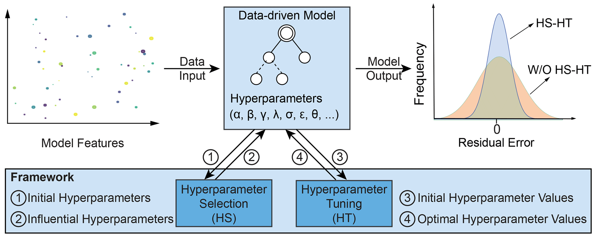
Figure 1 The methodological framework for improving the performance of data-driven models with two modules: hyperparameter selection (HS) and hyperparameter tuning (HT).

2.1 Hyperparameter selection

To understand the impact of individual hyperparameters and their interactions on the performance of a given data-driven model, we used a global sensitivity analysis (GSA) approach based on Sobol decomposition (Sobol, 2001), a variance decomposition technique. Through this GSA approach, the model output variance is decomposed into the summation of the variances from input parameters per se and their interactions. Let us assume that a data-driven model is of the form $\mathbf{Y}=\mathcal{M}(\mathit{X};\mathit{H})$, where X is a vector of features and $\mathit{H}=\mathit{\{}{h}_{\mathrm{1}},\mathrm{\dots },h_i,\mathrm{\dots },h_n\mathit{\}}$, a vector of hyperparameters, and h_i is the ith hyperparameter. We used 𝒪(Y) to define the scores of the objective function, 𝒪(Y), of the data-driven model, ℳ. By fixing the values of the features, X, and changing the values of the hyperparameters, H, the total variance of the score, denoted as V(𝒪(Y)), can be represented as the sum of the variance imposed by the individual hyperparameter, h_i, and its interactions with the other hyperparameters.

$$\begin{array}{}\text{(1)}& V\left(\mathcal{O}\right(Y\left)\right)=\sum _{i=\mathrm{1}}^n{V}_i+\sum _{i\le j\le n}^n{V}_{ij}+\mathrm{\dots }+V_{\mathrm{1},\mathrm{\dots },n},\end{array}$$

where V_i is the first order contribution of h_i to V(𝒪(Y)), and V_ij denotes the variance arising from the interactions between two hyperparameters, h_i and h_j. We can then measure the influence of a hyperparameter by its contribution to V(𝒪(Y)) using the sensitivity score of the first (S) and total order (ST) indices as follows:

$$\begin{array}{}\text{(2)}& {\displaystyle }{S}_i=V_i/V\left(\mathcal{O}\right(Y\left)\right)\text{(3)}& {\displaystyle }{\mathrm{ST}}_i=\mathrm{1}-V_{\sim i}/V\left(\mathcal{O}\right(Y\left)\right),\end{array}$$

where V_∼i indicates the contribution to V(𝒪(Y)) by all hyperparameters except h_i; S_i measures the direct contribution to V(𝒪(Y)) by h_i; and ST_i measures the contribution by h_i and its interactions, of any order, with all other hyperparameters.

To estimate S and ST, we first generated sufficient samples of the hyperparameters that can well represent the sample space. We chose the quasi-Monte Carlo sampling method (Owen, 2020), which uses quasi-random numbers (i.e., low discrepancy sequences) to sample points far away from the existing sample points. As such, the sample points can cover the sample space more evenly and quickly with the faster convergence rate of O((log N)^kN⁻¹), where N and k are the number and dimension of samples (Campolongo et al., 2011). In total, we generated m samples for n hyperparameters. We then fed the samples into the data-driven model, ℳ, to obtain the corresponding 𝒪(Y). Next, we estimated the variance components, V_i, V_∼i, and V(𝒪(Y)), in Eq. (1) with m(2n+2) model evaluations, and derived the scores of S_i and ST_i using Eqs. (2)–(3) (Saltelli, 2002). Finally, we selected the hyperparameters with high scores of the total order index as influential hyperparameters.

2.2 Hyperparameter tuning

After hyperparameter selection, we expect to tune fewer hyperparameters through hyperparameter optimization, which involves the process to maximize or minimize the score of the objective function, 𝒪(Y), of a data-driven model, ℳ, over the sample space of its hyperparameters, ℋ. As such, we can identify the optimal values of the hyperparameters, which are then used for training data-driven models.

Rather than manually tuning these hyperparameters, we chose to use an automated optimization approach, Bayesian hyperparameter optimization (Bergstra et al., 2011). This approach creates a surrogate model of the objective function using a probabilistic model. The surrogate model avoids solely relying upon local gradient and Hessian approximations by tracking the paired values of the hyperparameters and the corresponding scores of the objective function from previous trials and proposes new hyperparameters that can improve the score based on the Bayes rules. As such, this optimization approach can help avoid being trapped in the local optima and also requires far less time to identify the optimum of the hyperparameters, as the objective function can converge to a better score faster.

To describe the Bayesian optimization approach in more detail, let us assume that we have evaluated the objective function 𝒪(Y) for n sets of hyperparameters, $\mathit{\{}{h}^{\left(\mathrm{1}\right)},\mathrm{\dots },h^{\left(n\right)}\mathit{\}}$. Based on pairs of a set of hyperparameters and the corresponding score (h,𝒪(y)) from n evaluations, we applied a sequential model-based optimization (SMBO) method, a tree-structured Parzen estimator (TPE) (Bergstra et al., 2011), to develop a surrogate model for 𝒪(Y). The TPE defines the conditional probability, p(h|𝒪(y)), using two densities:

$$\begin{array}{}\text{(4)}& p\left(h\right|\mathcal{O}\left(y\right))=\left\{\begin{array}{ll}l\left(h\right)& \text{if}\mathcal{O}\left(y\right)<\mathcal{O}\left(y^{*}\right)\\ g\left(h\right)& \text{if}\mathcal{O}\left(y\right)\ge \mathcal{O}\left(y^{*}\right),\end{array}\right.\end{array}$$

where l(h) and g(h) can be modeled using different probability density or mass functions for continuous or discrete hyperparameters. For example, l(h) and g(h) can be a uniform, a Gaussian, or a log-uniform distribution for continuous hyperparameters. To define l(h), we use part of n sets of hyperparameters, {h⁽ⁱ⁾} that result in the score, 𝒪(y) less than the threshold, 𝒪(y^*) which is chosen to be some quantile γ of all scores, $p\left(\mathcal{O}\right(y)<\mathcal{O}(y^{*}\left)\right)=\mathit{\gamma }$; and g(h) is defined using the remaining hyperparameters (Bergstra et al., 2011).

The following step is to decide the next hyperparameter values that possibly give a better score, 𝒪(y) given the corresponding uncertainty measured by the surrogate model (Frazier, 2018). To do so, a selection function is defined based on the expected improvement (EI):

$$\begin{array}{}\text{(5)}& {\displaystyle }{\mathrm{EI}}_{\mathcal{O}\left(y^{*}\right)}\left(h\right):=\underset{-\mathrm{\infty }}{\overset{\mathcal{O}\left(y^{*}\right)}{\int }}\left(\mathcal{O}\right(y^{*})-\mathcal{O}(y\left)\right)p\left(\mathcal{O}\right(y\left)\right|h\left)d\mathcal{O}\right(y)\text{(6)}& {\displaystyle }\begin{array}{rl}& =\underset{-\mathrm{\infty }}{\overset{\mathcal{O}\left(y^{*}\right)}{\int }}\left(\mathcal{O}\right(y^{*})-\mathcal{O}(y\left)\right){\displaystyle \frac{p\left(h\right|\mathcal{O}\left(y\right)\left)p\right(\mathcal{O}\left(y\right))}{p\left(h\right)}}\\ & \times d\mathcal{O}\left(y\right),\end{array}\end{array}$$

where p(𝒪(y)|h) is parameterized as p(h|𝒪(y))p(𝒪(y)). It is set to zero when $\mathcal{O}\left(y\right)<\mathcal{O}(y*)$ in order to neglect all hyperparameters that yield no improvements in the score. Through maximizing EI, a better set of hyperparameters is identified. Together with the corresponding score, they are used to update the TPE, l(h), and g(h) for the maximization of EI. The iterative process continues until the maximum allowed number of iterations is reached.

2.3 Case study

The Maumee River watershed (Fig. 2) is the largest watershed in the Great Lakes region, covering more than 17 000 km² in Ohio, Indiana, and Michigan (U.S. Geological Survey, 2014). The watershed receives more than 800 mm of annual precipitation on average, with most of its rainfall from March to July and snowfall from December to March. The coldest and warmest months are February and July, respectively (NOAA National Centers for Environmental Information, 2012). The soil in the watershed is mainly composed of glacial till, which is a mixture of clay, silt, sand, and gravel deposited by glaciers; this type of soil is highly fertile but prone to erosion if not managed properly (NRCS-USDA, 2013). Owing to these excellent geophysical and humid continental climate conditions, over 70 % of the watershed is dedicated to agriculture, growing row crops such as corn, soybeans, and wheat (Kalcic et al., 2016). As such, fertilizer applied for crop growth in the watershed contributes over 77 % of total phosphorus (TP) entering the western basin of Lake Erie through the Maumee River (Kast et al., 2021; Maccoux et al., 2016).

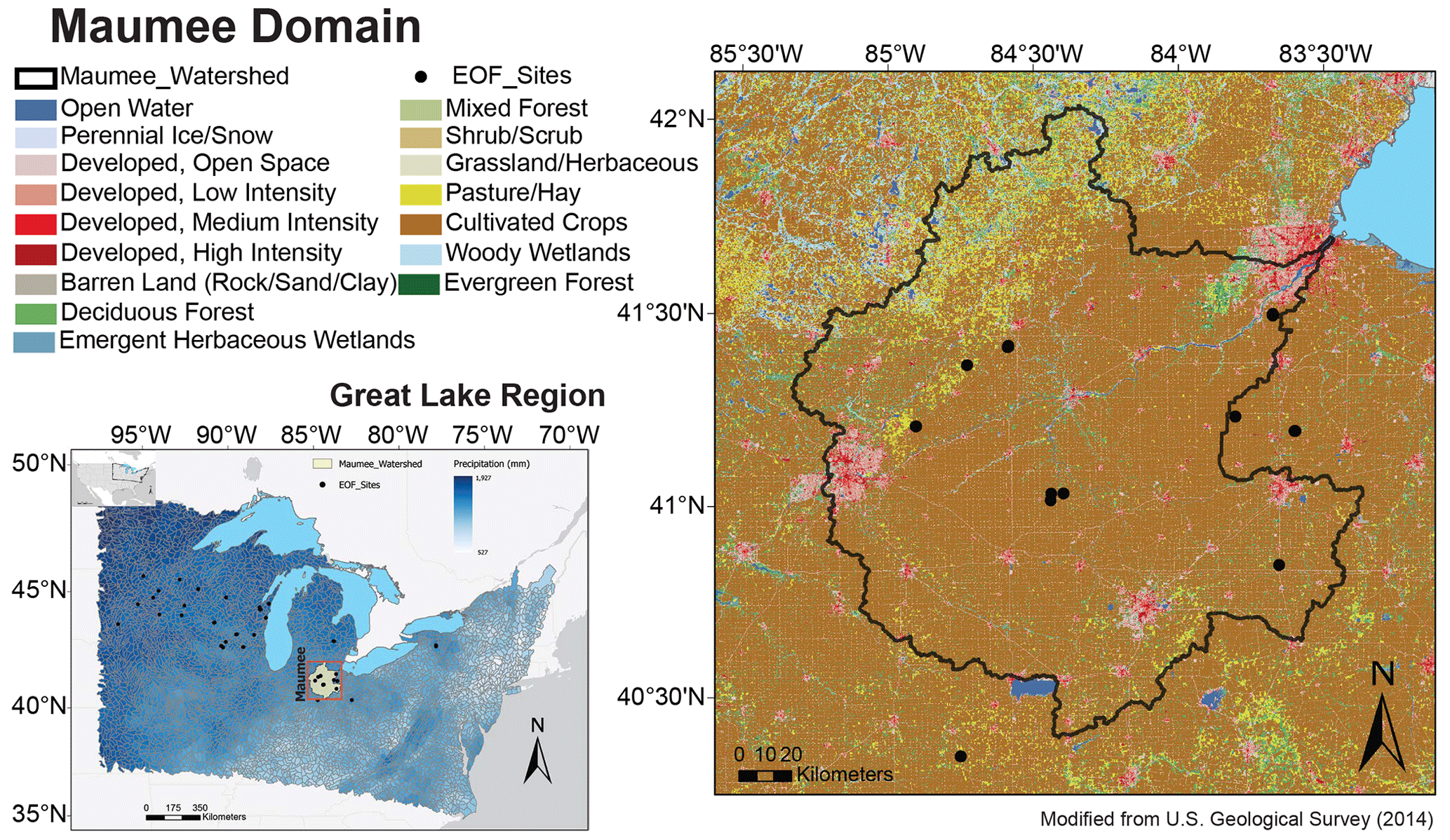
Figure 2 Study area of the Maumee domain in the Great Lakes region, USA. EOF sites (black dots) denote the locations where the observational data of daily edge-of-field (EOF) runoff is available over multiple years.

Agricultural runoff is the main source of non-point source pollution in the Maumee domain. The high nutrient load carried by edge-of-field (EOF) runoff from agricultural fields in the watershed has had detrimental effects on aquatic ecosystems, such as harmful algal blooms and hypoxia in Lake Erie (Scavia et al., 2019; Stackpoole et al., 2019). The occurrence and magnitude of EOF runoff can be influenced by many factors, but it is mainly driven by precipitation and snowmelt (Ford et al., 2022; Hu et al., 2021; Hamlin et al., 2020). An early warning system to forecast runoff risk can assist agriculture producers in the timing of fertilizer application to retain more nutrients in the land: this also reduces nutrient transport carried by runoff to nearby water bodies. To design such an early warning system, in the previous study (Hu et al., 2021), we developed a hybrid model to predict the magnitude of daily EOF runoff for all EOF sites in the domain (Fig. 2); the model combines National Oceanic and Atmospheric Administration's (NOAA) national water model (NWM) with a data-driven model based on the extreme gradient boosting algorithm (XGBoost; Chen and Guestrin, 2016). In this study, we will demonstrate the efficiency and effectiveness to train XGBoost models using the proposed framework (Fig. 1).

2.3.1 Data preparation

In this study, we used two types of datasets to train XGBoost models preceded by different approaches as illustrated in the framework (Fig. 1) and evaluated their performance of daily EOF runoff prediction at each EOF site in the study area. These two datasets include: (1) observations of daily EOF runoff at the EOF sites within the Maumee domain (Fig. 2) (this dataset was obtained from the conservation partners in the previous study (Hu et al., 2021)), and (2) daily values of the influential NWM model outputs. Based on the previous work on hybrid modeling using directed information for causal inference (Hu et al., 2021), we first calculated daily values of 72 NWM model outputs on the 1 km × 1 km grids where EOF sites are located and then identified seven influential outputs for the Maumee domain (Tables S1 and S2 in the Supplement). As we did not separate the winter season (i.e., from November to April) from the rest of the year when selecting influential variables, some of the selected influential outputs represented the driving forces of daily EOF runoff during the winter season, such as snow melt and soil temperature (Table S2 in the Supplement).

2.3.2 Implementation

Extreme gradient boosting (XGBoost) is a tree-based ensemble machine learning algorithm, which is mainly designed for its overall high convergence speed through optimal use of memory resources and good predictability through ensemble learning that leverages the combined predictive power of multiple tree models (Chen and Guestrin, 2016). Using the gradient boosting technique, XGBoost incorporates a new tree model (i.e., weak learner) into the tree ensemble models obtained from previous iterations in a repetitive manner. At the tth iteration, an objective function, J, is defined as

$$\begin{array}{}\text{(7)}& {\displaystyle }{\displaystyle }{J}^{\left(t\right)}=\sum _{i=\mathrm{1}}^{n}L(y_i,\widehat{y_i})+\sum _{m=\mathrm{1}}^{t}R\left(f_m\right),\end{array}$$

where n is the number of samples and L is the training loss function; $\widehat{y_i}$ is the prediction from the tree ensemble models ℱ; $\widehat{y_i}={\sum }_{i=\mathrm{1}}^m{f}_m\left(x_i\right),f_m\in F$, and m are the number of tree models; and R is the regularization function used to penalize the complexity of the tree ensemble models to reduce model overfitting. All these functions are characterized by a set of hyperparameters, e.g., learning rate (LR) and maximum tree depth (MD). Through optimizing J, an XGBoost model can be obtained with locally optimal hyperparameter values, which gives the best predictive performance at the ith iteration. The process iterates for a defined number of repetitions to train the XGBoost model that can balance model bias and variance error.

The XGBoost algorithm has been demonstrated to be effective for a wide range of regression and classification problems, such as overfitting and imbalanced datasets (Dong et al., 2020). In this study, we used XGBoost models to predict the magnitudes of daily EOF runoff in the Maumee domain (Fig. 2). We considered nine hyperparameters associated with the XGBoost algorithm (Fig. 3). Daily EOF measurements within the watershed (Hu, 2022a) were used for hyperparameter selection, and the score 𝒪(y) of the objective function was measured by the mean absolute error (MAE; Sect. 2.3.3). We then modified the Python SALib package (Herman and Usher, 2017), which was developed for Sobol-based global sensitivity analysis only with model features and parameters; such modification allows the calculation of sensitivity scores for hyperparameters (i.e., the HS approach). Given the number and range of the hyperparameter values, and the complexity of the XGBoost model, we generated 4000 samples of hyperparameters (Fig. 3a) to calculate the S and ST values for all nine hyperparameters, and we selected the influential ones given their ST values.

After the influential hyperparameters were identified, the next step was to search the optimal values for these hyperparameters through hyperparameter tuning (i.e., the HT approach). To do so, we first randomly selected 70 % of the EOF datasets within the domain. Based on the selected data, we then used the Bayesian optimization (BO) approach implemented via the Python Hyperopt library (Bergstra et al., 2013) to identify the optimal hyperparameter values. Given these optimal values, we trained and evaluated XGBoost models in predicting the magnitude of daily EOF runoff at the EOF sites in the domain (Hu et al., 2021). Additionally, to evaluate the impact of hyperparameter selection on model performance, we trained and evaluated the performance of XGBoost models without hyperparameter selection, that is, using only hyperparameter tuning on the initial set of hyperparameters. To further mitigate the impact of the imbalanced runoff data, besides the effective XGBoost algorithm, we used the stratified k-fold cross-validation (Kohavi, 1995) across different scenarios to ensure the training and test datasets follow a similar distribution, and we defined a loss function (e.g., R squared) that penalizes more the missing predictions of large runoff events, that is, the minority class in this study.

2.3.3 Evaluation metrics

In this study, we used mean absolute error (MAE) to measure the score of the objective function 𝒪(Y), and R squared (R²) to measure the level of agreement between the predictions from the XGBoost models and observations of daily EOF runoff.

$$\begin{array}{}\text{(8)}& {\displaystyle }\mathrm{MAE}={\displaystyle \frac{\mathrm{1}}{n}}\sum _{i=\mathrm{1}}^n|y_i-\widehat{y_i}|\text{where}\mathrm{MAE}\in [\mathrm{0},+\mathrm{\infty }],\text{(9)}& {\displaystyle }\begin{array}{rl}{R}^{\mathrm{2}}& ={\displaystyle \frac{({\sum }_{i=\mathrm{1}}^n\widehat{y_i}{y}_i-n\stackrel{\mathrm{‾}}{\widehat{Y}}\stackrel{\mathrm{‾}}{Y}{)}^{\mathrm{2}}}{({\sum }_{i=\mathrm{1}}^n{\widehat{y_i}}^{\mathrm{2}}-n{\stackrel{\mathrm{‾}}{\widehat{Y}}}^{\mathrm{2}})({\sum }_{i=\mathrm{1}}^n{y_i}^{\mathrm{2}}-n{\stackrel{\mathrm{‾}}{Y}}^{\mathrm{2}})}}\\ & \text{where}{R}^{\mathrm{2}}\in [-\mathrm{\infty },\mathrm{1}],\end{array}\end{array}$$

where n is the sample size; y_i and $\widehat{y_i}$ are the observed and predicted value of daily EOF runoff for a specific EOF site, respectively; and $\stackrel{\mathrm{‾}}{Y}$ and $\stackrel{\mathrm{‾}}{\widehat{Y}}$ are the mean values of y_i and $\widehat{y_i}$, respectively. The MAE value equal to zero is the perfect score, whereas the R² value closer to one is considered to be the perfect agreement between predictions and observations.

3 Results

The ability to represent the search space of all nine hyperparameters by the selected samples is critical to estimating their influence on the model performance through the sensitivity analysis approach. In our case, we have selected 4000 samples in total. As shown by the histogram plots on the diagonal in Fig. 3a, the entire range of values for each hyperparameter is well represented by uniformly distributed intervals of values. Additionally, the well-scattered sample points on the off-diagonal plots indicate no correlation among each other, confirming the independence between these hyperparameters and the appropriate samples to use for hyperparameter selection.

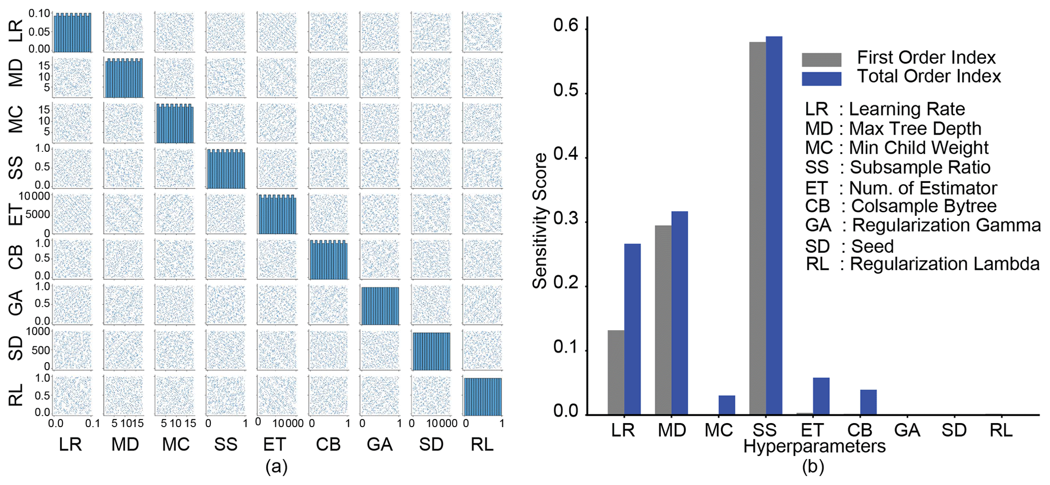
Figure 3 (a) Samples of nine hyperparameters associated with the extreme gradient boosting (XGBoost) algorithm for the global sensitivity analysis. The histogram plots on the diagonal describe the actual sample distribution for a given hyperparameter. Each bar in the histogram plots measures the sample size in the corresponding interval. (b) Comparison of the sensitivity scores of the nine hyperparameters for both first (gray) and total (blue) order Sobol indices.

Through hyperparameter selection, the influence of hyperparameters is ranked by their contributions to the variance of the objective function, characterized by the sensitivity score of the total order index, ST (Fig. 3b). The higher the score, the more influential the hyperparameter is. Among the nine hyperparameters for the XGBoost model, the subsample ratio of the training data, SS, is the most influential hyperparameter with the highest sensitivity score for both S and ST, followed by the maximum tree depth, MD, and the learning rate, LR (Fig. 3b). We noticed small differences in sensitivity score between S and ST for the first two most influential hyperparameters, SS and MD, indicating that the contributions to their ST scores are made by the variation of the hyperparameters per se. In contrast, for the hyperparameter, LR, a large portion of its high ST score is contributed through the interaction between LR and the other hyperparameters. As a result, instead of tuning all hyperparameters, we only need to search for the optimal values of these three influential hyperparameters through hyperparameter tuning.

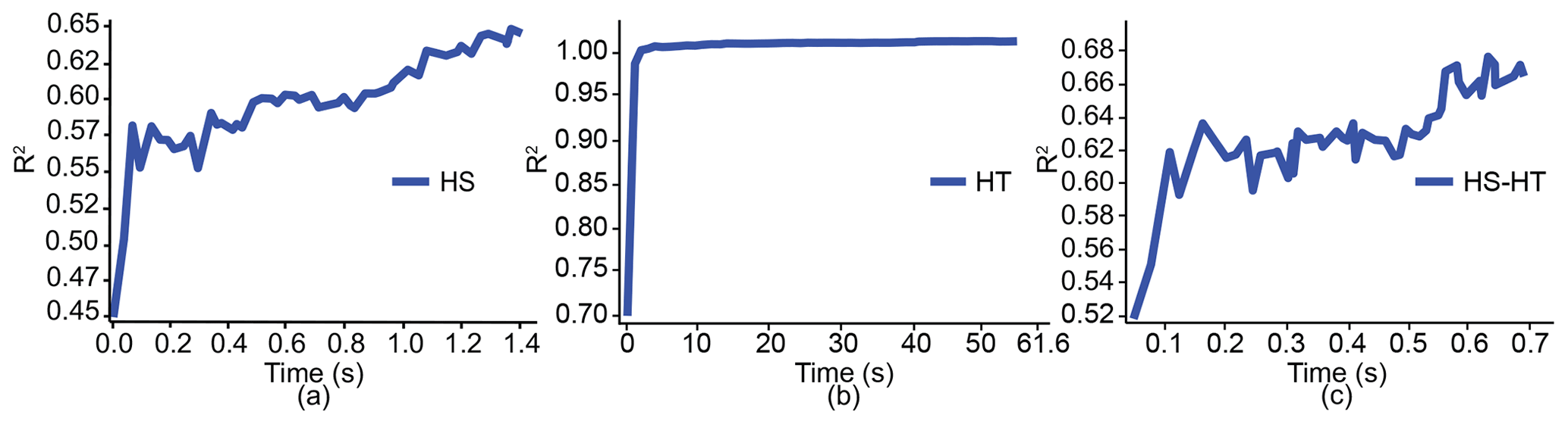
Figure 4 Comparison of the training time for the XGBoost models using hyperparameter selection (HS), hyperparameter tuning (HT), and both of them (HS–HT), as proposed by the framework with respect to their performance measured by R² over 8000 iterations.

We trained XGBoost models for the prediction of daily EOF runoff events in the study domain (Fig. 2) with a fixed number of iterations (i.e., 8000 in our case). We noticed that the training of XGBoost models preceded by our proposed framework, the combination of hyperparameter selection and tuning (i.e., the HS–HT approach), took the least time (0.7 s; Fig. 4c) compared to the training of models preceded by either the HS or HT approach (1.4 and 61.6 s; Fig. 4a and b). Similar to the case with only the HS approach, the performance of the XGBoost model steadily improved during training when the HS–HT approach was used, i.e., R² increased from 0.52 to 0.68. In contrast, when only the HT approach is used, the model quickly achieved almost perfect performance (i.e., close to R²=1.0) but gained small improvements over the rest of the training. In this regard, the training process after the HT approach was not as effective compared to that using the HS–HT approach, although the former achieved better training performance.

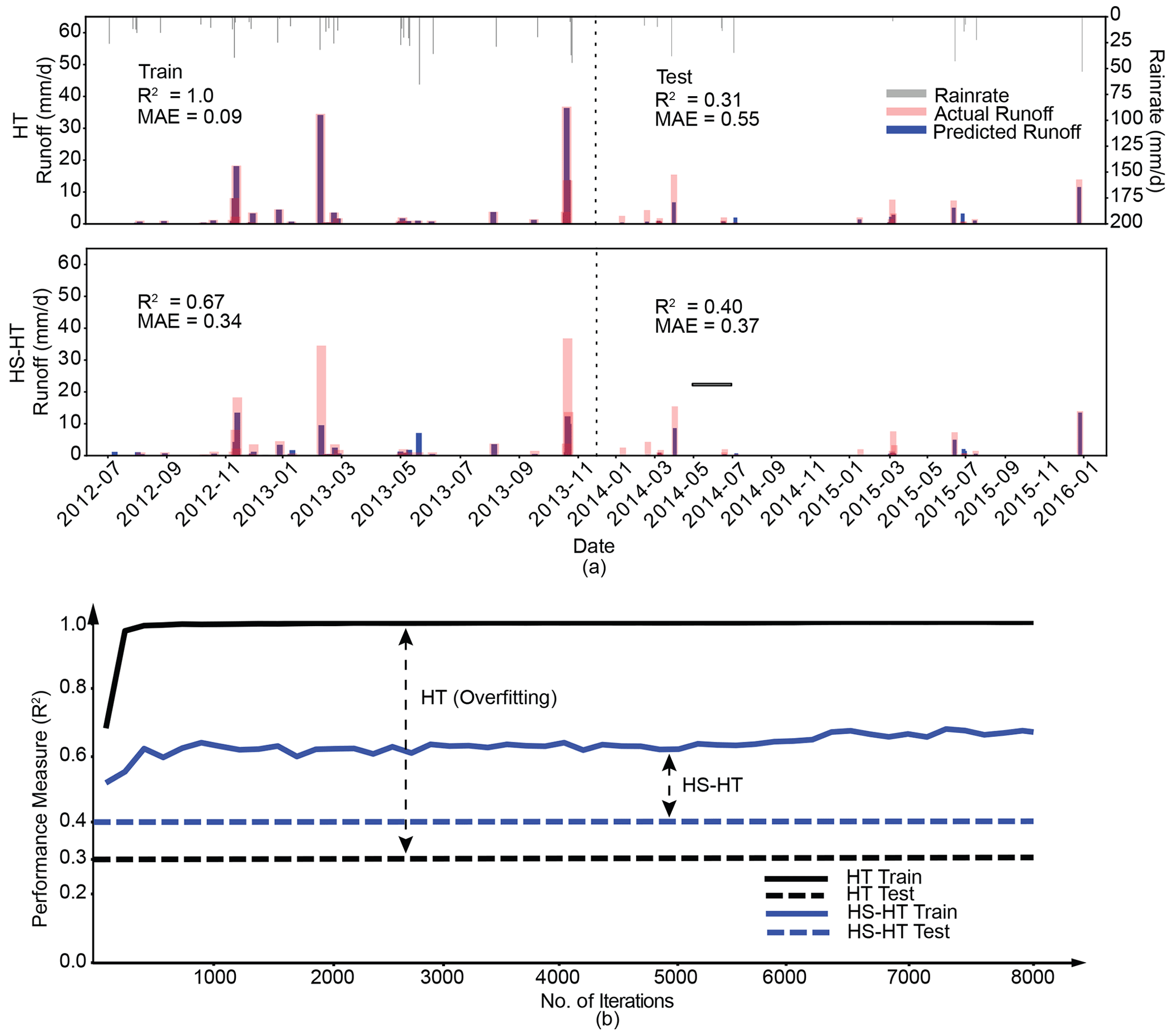
Figure 5 (a) Comparison of the performance of the XGBoost models in prediction of daily EOF runoff for the Maumee domain with respect to the observed runoff preceded by the HT approach and the proposed framework (i.e., the HS–HT approach) for a given period. The upper x axis shows the rainfall intensity (mm d⁻¹) over the training (July 2012–December 2013) and test (January 2014–January 2016) period, respectively. (b) Comparison of the performance of the XGBoost models preceded by the two approaches, HS–HT and HT, with respect to the number of iterations. The double-headed arrows indicate the differences in R² values between the training and test for each approach.

However, better training performance cannot guarantee a better test performance due to the risk of overfitting. For the Maumee domain (Fig. 2), the XGBoost model achieved an almost perfect agreement with the observations (R²=1.0) when preceded by the HT approach, while having a relatively poor performance in test with R²=0.31 (Fig. 5a), representing a 69.0 % reduction in performance. On the contrary, the XGBoost model performed worse in training when preceded by the proposed framework (i.e., the HS–HT approach) with R²=0.67 but produced a better test performance (R²=0.40), resulting in a smaller performance reduction of 40.3 %.

Similarly, we also evaluated the overfitting of the resulting XGBoost models by directly measuring the gaps between the model performances in training at different numbers of iterations and their test performances (Fig. 5b). Please note that once XGBoost models are trained, their test performances become irrelevant to the number of iterations during the training process and thus stay constant (Fig. 5b). We noticed that the model preceded by the HT approach was more prone to overfitting, since the gaps measured by the differences in R² values were always larger than the gaps for the case with the proposed framework. As such, it demonstrated that the proposed framework can help reduce model overfitting.

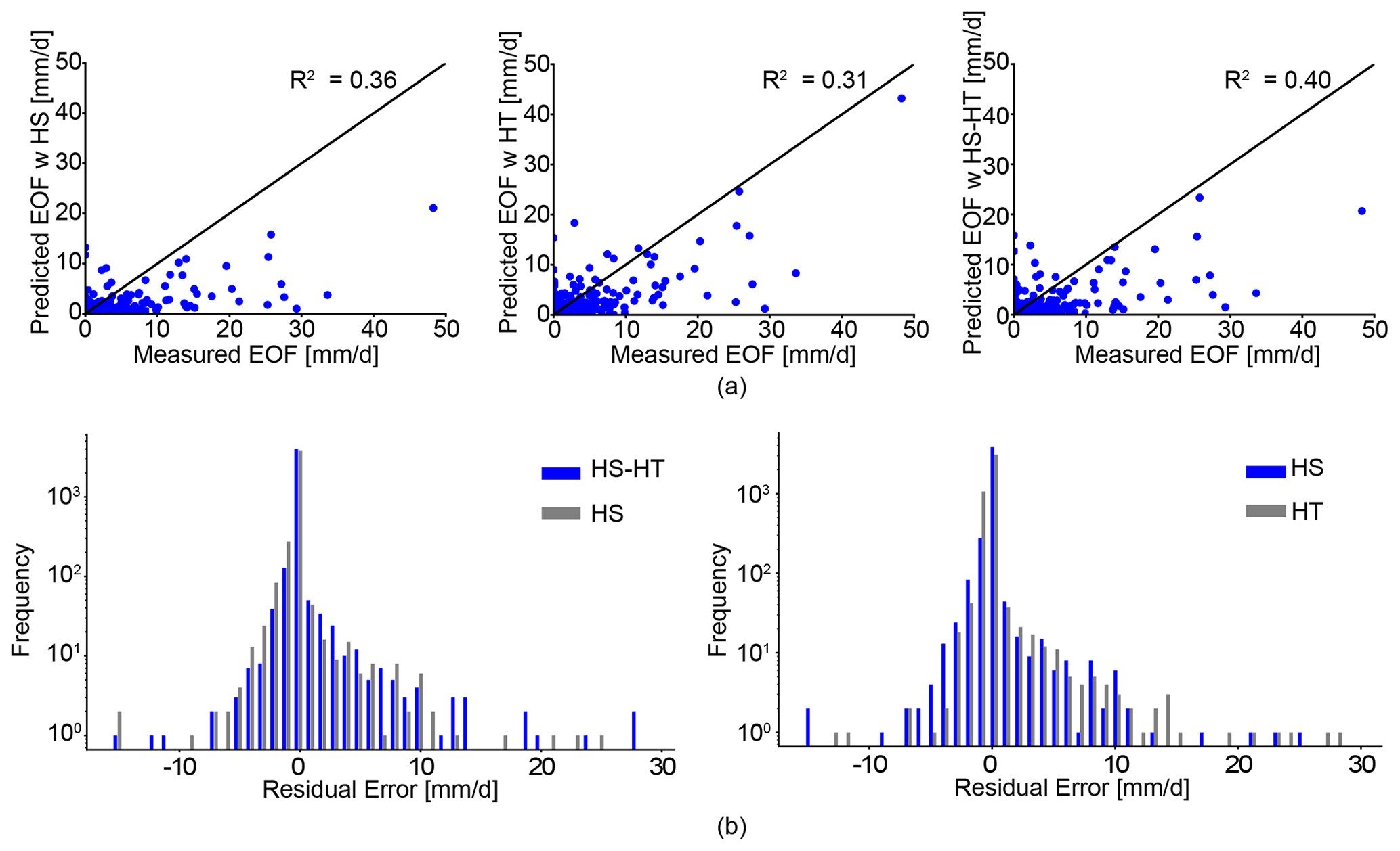
Figure 6 (a) Comparison of the observations with the predictions of daily EOF runoff for the Maumee domain by the XGBoost models trained using the HS, HT, and HS–HT approaches, respectively. (b) Comparison of residual errors between the observations and the predictions of daily EOF runoff for the Maumee domain by the XGBoost models trained using the HS–HT, HS, and HT approaches, respectively.

As shown by Fig. 6a, using the proposed framework (i.e., the HS–HT approach), the resulting XGBoost model achieved a better agreement with the observations (R²=0.40) than the corresponding XGBoost models preceded by other approaches (R²=0.36 for the HS approach, R²=0.31 for the HT approach). We noticed the relative difference in model performance for the HS and HS–HT approaches (in terms of R² value) is smaller than the difference for the HT and HS–HT approaches. In this regard, the XGBoost model had the worst performance if only the HT approach was used to search for the optimal values for all hyperparameters. This is further demonstrated by the comparison of residual errors between the observations and predictions of then XGBoost models preceded by different approaches (Fig. 6b): for the HS–HT approach, residual errors are more concentrated around the zero value compared to the wider scatter of errors as the result of using only the HS or HT approach, respectively. As such, the XGBoost models can often achieve better test performance when preceded by the proposed framework.

4 Discussion

In this section, we will discuss the effects of the proposed framework using hyperparameter selection and tuning on model training and the overall performance of XGBoost models. Through the discussion below, we aim to demonstrate that the results gained from this study are generally applicable to other data-driven models.

4.1 Influence of hyperparameters

In this study, we conducted the Sobol-based global sensitivity analysis (i.e., the HS approach) to identify the influential hyperparameters of XGBoost models. We identified three influential hyperparameters for the XGBoost model based on their sensitivity scores of the total order index (i.e., ST) and their relative differences from the first order index (i.e., S). Among them, the maximum tree depth, MD, and the learning rate, LR, are often considered important hyperparameters for XGBoost models, since LR is associated with model convergence and MD controls the depth of the tree model. As the depth of the tree increases, the tree model contains more inner layers, enabling it to better learn complex, non-linear patterns from the data. However, tree models with greater depth are also more prone to overfitting.

For the learning rate (LR), a higher learning rate often leads to faster training, but the resulting tree models are more likely to reach suboptimal solutions. In contrast, models with a low learning rate converge slowly but are likely to have good performance with optimal hyperparameter values. Additionally, around half of its influence measured by ST is the result of interactions with other hyperparameters (Fig. 3). For such a hyperparameter, we need to investigate if other hyperparameters with low ST scores should also be considered influential due to their interactions with the target hyperparameter. In our case, we decided not to consider others, mainly because the S score of the learning rate is already much higher than the ST score of the next one in the rank, i.e., the number of tree estimators, ET.

Although these two hyperparameters are considered influential in the current study, the most influential hyperparameter is the subsample ratio (SS) of the training data, which determines the sample size used to grow a new tree model in each boosting iteration. This is possibly due to the imbalanced data of the target variable, the daily EOF runoff, which is often zero-inflated with sparsely distributed runoff events over a long time horizon. The number of non-zero EOF runoffs in the training set, determined by the subsample ratio, can affect the model performance. With more zero values included in the dataset, fewer non-zero EOF runoffs are available to support model training, and vice versa. As such, the subsample ratio appears to be the most critical hyperparameter for the performance of the XGBoost model in the study. Similar to the sensitivity analysis of physics-based models, analysis results depend on the characteristics of the target variable (e.g., the daily EOF runoff in our case). As such, for applications involving data-driven models, we can first rely on our experience to select the hyperparameters and then refine the list of influential hyperparameters using the proposed HS approach.

4.2 Algorithm complexity and model training

Data-driven models perform differently in training with and without hyperparameter selection. In general, models with more hyperparameters are more capable of learning complex, non-linear relationships from data. In our case study, XGBoost models were initially set up with nine hyperparameters (Fig. 3) to account for the complexity of daily EOF runoff prediction (Hu et al., 2021). This explains why the XGBoost model without hyperparameter selection can often achieve very good training performance (Fig. 4). However, fast convergence to good training performance indicates that data patterns can be too easy for the model to learn. Furthermore, after the initial significant improvement, the performance of the XGBoost model levels off for the majority of the training time. In this regard, the whole training is not effective, using additional training time on almost negligible improvements.

After hyperparameter selection, three out of nine hyperparameters are considered influential to the prediction of daily EOF runoff, which allows model training with a less complex XGBoost algorithm for the search of optimal model parameter values. For this reason, given the same number of iterations for training, it is thus more efficient to train the model after hyperparameter selection in terms of training time (Fig. 4). Meanwhile, guaranteed by the HS approach, the removal of non-influential hyperparameters will have no or limited impact on model performance in the EOF runoff prediction. Training can also be more effective, as demonstrated by the steady improvement of the XGBoost model during the training period. As such, through hyperparameter selection, the resulting XGBoost model, equipped with fewer but influential hyperparameters, can be trained more efficiently and effectively to predict the target variable, e.g., the daily EOF runoff over the Maumee domain.

Meanwhile, XGBoost models also perform differently in training with and without hyperparameter tuning. When training an XGBoost model without the HT approach, we assign values to the hyperparameters by trial and error. The resulting XGBoost algorithm is likely not to be optimal and thus can take longer time to search for the optimal values for the model parameters compared to the case using hyperparameter optimization; this is demonstrated by the faster convergence to better performance when training is preceded by the HS–HT approach compared to that by the HS approach alone (Fig. 4a and c). Nevertheless, model training preceded by the HS approach is still more effective compared to that using the HT approach alone (Fig. 4a and b). This can be because the XGBoost algorithm with more hyperparameters (without hyperparameter selection) can more easily learn the pattern from data, resulting in no improvement in training for the majority of the training time. As such, the combination of the HS and HT approach as proposed by the framework can most effectively improve search efficiency.

4.3 Model overfitting and performance

The complexity of the underlying machine learning algorithm can be characterized by the number of hyperparameters and their values, which are critical to the model performance. High algorithm complexity can often result in overfitted models, as demonstrated by the large model performance gap in training and test (Fig. 5a and b). Through the identification of influential hyperparameters, the HS approach helps reduce the algorithm complexity by using an appropriate number of hyperparameters that can balance the prediction errors and variance in the dataset. As a result, reduction of algorithm complexity through the removal of non-influential hyperparameters can effectively reduce model overfitting without compromising model performance, which is further guaranteed by the use of the HT approach, searching optimal values for these influential hyperparameters.

4.4 Limitation and outlook

The framework is designed to reduce model training time and improve model performance, which is done through the identification of influential hyperparameters and their optimal values. Please note that the specific results for hyperparameter selection and tuning are data- and domain-specific, and the impact of data size, quality, and location is not yet fully explored in this study. Additionally, previous work (Hu et al., 2018) has demonstrated the importance of feature selection for model performance in terms of model training time and overfitting. Thus, it is worth investigating the performance of data-driven models when the framework is combined with feature selection.

5 Conclusions

In this paper, we developed a framework composed of hyperparameter selection and tuning, which can effectively improve the performance of data-driven models by reducing both model training time and model overfitting. We demonstrated the framework efficacy using a case study of daily EOF runoff prediction by XGBoost models in the Maumee domain, USA. Through the use of Sobol-based global sensitivity analysis, hyperparameter selection enables the reduction in complexity of the XGBoost algorithm without compromising its performance in model training. This further allows hyperparameter tuning using a Bayesian optimization approach to be more effective in searching the optimal values only for the influential hyperparameters. The resulting optimized XGBoost algorithm can effectively reduce model overfitting and improve the overall performance of XGBoost models in the prediction of daily EOF runoff. This framework can thus serve as a useful tool for the application of data-driven models in EESs.