Importance of ice nucleation and precipitation on climate with the Parameterization of Unified Microphysics Across Scales version 1 (PUMASv1)

Cloud microphysics is critical for weather and climate prediction. In this work, we document updates and corrections to the cloud microphysical scheme used in the Community Earth System Model (CESM) and other models. These updates include a new nomenclature for the scheme, now called Parameterization of Unified Microphysics Across Scales (PUMAS), and the ability to run the scheme on graphics processing units (GPUs). The main science changes include refactoring an ice number limiter and associated changes to ice nucleation, adding vapor deposition onto snow, and introducing an implicit numerical treatment for sedimentation. We also detail the improvements in computational performance that can be achieved with GPU acceleration. We then show the impact of these scheme changes on the (a) mean state climate, (b) cloud feedback response to warming, and (c) aerosol forcing. We find that corrections are needed to the immersion freezing parameterization and that ice nucleation has important impacts on climate. We also find that the revised scheme produces less cloud liquid and ice but that this can be adjusted by changing the loss process for cloud liquid (autoconversion). Furthermore, there are few discernible effects of the PUMAS changes on cloud feedbacks but some reductions in the magnitude of aerosol–cloud interactions (ACIs). Small cloud feedback changes appear to be related to the implicit sedimentation scheme, with a number of factors affecting ACIs.

1 Introduction

Cloud microphysics is critical for weather and climate. In particular, supercooled liquid water (liquid at temperatures below 0 ^∘C) and the fraction of condensate in the form of supercooled liquid at high latitudes has been shown to be important for mean state climate (Bodas-Salcedo et al., 2019) and weather (Forbes et al., 2015) biases. Supercooled liquid water is also important for understanding cloud feedbacks and climate sensitivity (Tan et al., 2016; Gettelman et al., 2019b; Tan and Storelvmo, 2019). For example, the Community Earth System Model version 2 (CESM2; Danabasoglu et al., 2020) has been shown to have a higher supercooled liquid fraction than observed (Gettelman et al., 2020), which has been linked to a higher climate sensitivity than previous versions (Gettelman et al., 2019b). In addition, cloud microphysics controls the formation of precipitation, which is often too light and too frequent in large-scale weather and climate models (Stephens et al., 2010). This frequency bias has been shown to be directly attributable to cloud microphysics (Gettelman et al., 2021). In this work, we describe adjustments and corrections to the ice microphysics and precipitation process in an advanced cloud microphysics scheme used in several global models and how these changes can have a significant effect on simulated climate.

The state of the art for global model cloud microphysics is the use of bulk two-moment schemes, such as the scheme developed by Morrison and Gettelman (2008, MG1). The CESM2 atmosphere model uses cloud microphysics described by Gettelman and Morrison (2015) and Gettelman et al. (2015), termed MG2 (Morrison–Gettelman version 2). The scheme has been updated further to include rimed ice by Gettelman et al. (2019a, MG3). Most two-moment bulk schemes utilize classes of hydrometeors (such as cloud liquid, cloud ice, and snow). In such schemes, number and mass are predicted for each class, and hydrometeors are treated using a size distribution with a fixed functional form. Two-moment schemes are widely used in mesoscale models (e.g., Thompson and Eidhammer, 2014) at resolutions of a few kilometers but less commonly used in global models (e.g., Lohmann et al., 1999, 2007; Michibata et al., 2019). The scheme of Morrison and Milbrandt (2015) uses a single hydrometeor class to represent all ice particles, thereby unifying the treatment of cloud ice and snow, and was implemented in the MG1 scheme by Eidhammer et al. (2016).

Our purposes in this paper are several. First, we document updates and corrections to the MG3 cloud microphysical scheme used in CESM2. These include a new nomenclature for the scheme and the ability to run the scheme on graphics processing units (GPUs). We detail the improvements in computational performance that can be achieved with GPU acceleration. We then show the impact of the changes and corrections on (a) mean state climate, (b) cloud feedback response to warming, and (c) aerosol forcing. Note that we are not presenting a new set of tuned model configurations at this time. Rather, we show the impacts of changes and improvements in the scheme, particularly related to ice and mixed-phase processes, with the goal of building toward a cloud physics scheme that can work across scales (as shown in Gettelman et al., 2019c).

We describe the model and microphysics scheme updates in Sect. 2. Section 3 describes the methodology, simulations and evaluation. Section 4 presents results, and Sect. 5 has discussion and conclusions.

2 Model description

2.1 Model description – CESM2

CESM2 (Danabasoglu et al., 2020) features the Community Atmosphere Model version 6 (CAM6) as its atmosphere model. CAM6 uses a two-moment stratiform cloud microphysics scheme MG2 (Gettelman and Morrison, 2015; Gettelman et al., 2015) with prognostic liquid, ice, rain, and snow hydrometeor classes. As a two-moment bulk scheme, MG2 has prognostic variables for number- and mass-mixing ratios for each of the hydrometeor classes. It also permits ice supersaturation and is described further below.

MG2 is also coupled to a four-mode aerosol model (Liu et al., 2016) with liquid activation, following Abdul-Razzak and Ghan (2002), and features natural and anthropogenic aerosols. CAM6 includes a physically based mixed-phase ice nucleation scheme (Hoose et al., 2010) and accounts for preexisting ice for nucleation (Shi et al., 2015). MG2 is coupled to a unified moist turbulence scheme, Cloud Layers Unified By Binormals (CLUBB; Golaz et al., 2002; Larson et al., 2002), implemented in CAM by Bogenschutz et al. (2013). CLUBB treats boundary layer moist turbulence, stratiform clouds, and shallow cumulus. CAM6 uses an ensemble plume mass flux deep convection scheme (Zhang and McFarlane, 1995; Neale et al., 2008) with simple microphysics. The radiation scheme is the rapid radiative transfer model for general circulation (RRTMG) models (Iacono et al., 2000).

2.2 Cloud microphysics

MG2 (Gettelman and Morrison, 2015) is an update of the original MG scheme (Morrison and Gettelman, 2008; Gettelman et al., 2008). The original MG scheme was implemented in CAM5, as described by Gettelman et al. (2010). MG2 added prognostic rain and snow and is used in CAM6. Many of the process rate treatments are similar to the bulk two-moment microphysics scheme of Morrison et al. (2005) developed for mesoscale models. Gettelman et al. (2019a) further updated the MG2 scheme to MG3 by adding rimed ice (with a switch to represent either graupel or hail). Thus, MG3 includes two additional prognostic variables for graupel/hail number- and mass-mixing ratios. In a separate work, Eidhammer et al. (2016) and Zhao et al. (2017) updated the scheme to use a single category for cloud ice and snow. This has not been implemented yet in MG2 or MG3, and the integration is a subject for future work.

Versions of MG microphysics have been adapted for use in the NASA GEOS (Goddard Earth Observing System with an integrated Earth system model; Barahona et al., 2014), the Geophysical Fluid Dynamics Laboratory (GFDL) Atmosphere Model (AM; Salzmann et al., 2010), and the NASA Goddard Institute for Space Studies (GISS) model (Cesana et al., 2019). The scheme is also available in the idealized kinematic driver (KID; Shipway and Hill, 2012; Gettelman et al., 2019a). MG1 and MG2 are also used in a suite of Earth system models derived from CESM1 and CESM2. Analyses have been conducted against observations for sub-grid-process rate formulations (Lebsock et al., 2013) and against in situ aircraft flights for supercooled liquid water (Gettelman et al., 2020). There has been significant work on numerical time-stepping issues detailed by Gettelman and Morrison (2015) and Santos et al. (2020).

There are now a large number of people contributing to the community development of the MG scheme. Thus, the MG name is no longer appropriate, and we are now naming the scheme the Parameterization for Unified Microphysics Across Scales (PUMAS). This work describes the updates and changes from MG3 to PUMAS (version 1).

As part of this update, we have tested and implemented several science and software changes to PUMAS beyond the MG3 scheme (Gettelman et al., 2019a). These changes are as follows:

1. refactoring the ice number limiter,

2. reducing the aerosol number for ice nucleation,

3. allowing the vapor depositional growth of snow,

4. correcting the fall speed for rain, snow, and/or graupel,

5. giving an option for implicit sedimentation calculation,

6. providing an option for cloud droplet accretion by rain to act on newly autoconverted rain,

7. adding OpenACC (GPU accelerator) directives, and

8. having optional switches to replicate processes in the European Centre for Medium-Range Weather Forecasts (ECMWF) Integrated Forecasting System (IFS).

2.2.1 Ice number limiter

In all versions of MG microphysics, a cloud ice number limiter is applied such that, when integrated over the time step, ice nucleation cannot increase the total ice concentration beyond the concentration of available ice-nucleating particles (INPs). This approach limits ice number from all processes, except the sedimentation and homogeneous freezing of cloud and rain drops. The concentration of available INPs in this approach, NIMAX, includes the Liu and Penner (2005) homogeneous NIHOM and heterogeneous NIHET cirrus ice nucleation and the empirical Meyers et al. (1992) ice nucleation as a function of temperature for the mixed phase NIMEY as follows:

$$\begin{array}{}\text{(1)}& \text{NIMAX}=\text{NIHET}+\text{NIHOM}+\text{NIMEY}.\end{array}$$

When the Hoose and Möhler (2012) scheme based on classical nucleation theory (CNT) was introduced in CAM6, and the Meyers et al. (1992) ice nucleation removed, then the ice nucleation source from Hoose and Möhler (2012), NICNT, comprising immersion, deposition, and contact freezing terms, was not added to NIMAX (the equation above was unchanged). In addition, the ice nucleation source from Meyers et al. (1992) was set to zero (NIMEY=0). As a result, NIMAX in the mixed-phase regime (where NICNT>0) is too low, preventing the model from adding ice crystals through local nucleation as intended.

The reduced NIMAX leads to lower ice number concentration and, hence, increased size and increased fall speed and loss through sedimentation (Shaw et al., 2022), as well as affecting the balance of ice and supercooled liquid at high latitudes. In CAM6, this increases the supercooled liquid fraction when the NIMAX limiter is removed (Shaw et al., 2022). The CAM6-simulated supercooled liquid fraction is higher than observed in key regions (Gettelman et al., 2020). The supercooled liquid fraction and ice nucleation have been implicated in altering cloud feedbacks and climate sensitivity (Gettelman et al., 2019b; Tan and Storelvmo, 2019), suggesting that how the ice number limiter is applied may be important.

In this update (all simulations but the control), the NIMAX limiter on ice nucleation has been removed, and instead, an overall cap on the in-cloud ice number concentration is added to the end of the microphysics (set at 100 cm⁻³ to represent a maximum typical ice crystal number found in deep clouds). At small scales, measurements have shown much higher concentrations, up to ∼50 cm⁻³, embedded within broader regions with much lower concentrations <1 cm⁻³ (e.g., Hoyle et al., 2005). Satellite retrievals also show lower concentrations (up to several hundred per liter) over broad regions (e.g., Gryspeerdt et al., 2018). The main point is that we want to set this upper limit for ice concentration NIMAX to a large value such that it encompasses the range of physical values – in general, we want the process parameterizations to control the ice concentration rather than NIMAX and only impose the limit to ensure that the values are within a physically reasonable range. This is similar to the ice number concentration limiter applied to many two-moment microphysics schemes in cloud and mesoscale models (Morrison et al., 2005; Milbrandt and Yau, 2005; Thompson and Eidhammer, 2014). Zhu et al. (2022) implemented a similar change to develop a version of CESM2 for use in paleoclimate applications.

2.2.2 Reduced aerosol number for ice nucleation

When the ice number limiter is refactored, the immersion freezing component of the CNT mixed-phase ice nucleation scheme of Hoose et al. (2010) was found to produce an unrealistically high number of ice crystals near the low end of the mixed-phase temperature range (−38 ^∘C), heavily concentrating ice crystals in the mid-to-upper atmosphere near desert regions (sources of mineral dust that act as ice-nucleating particles) to an extent not evident in satellite retrievals (Sourdeval et al., 2018; McGraw et al., 2022). Figure 1b illustrates the large increase in ice number when PUMAS is implemented with the original MG2 CNT immersion freezing (MG2 Imm). Accordingly, we make two adjustments to the scheme to reduce aerosol number (particularly dust) involved in ice nucleation. First, instead of calculating the number fraction for dust and BC based on observed field measurements of dust size distributions, we calculate the number fraction from the mass fraction of the aerosols for immersion freezing. Second, we allow only a fraction of the dust to nucleate (5 %), similar to what is already done for black carbon (1 % used), following McGraw et al. (2022). The results are illustrated in Fig. 1c, where the ice number concentrations look more similar to the control simulation (note that the difference scale is a factor of 10 lower in Fig. 1c than in Fig. 1b), but there still is some immersion freezing active (see below). A complete explanation for the excessive ice nucleation at the edge of the applied temperature range for CNT is a subject of future work. However, one possibility is that, without considering a full aerosol budget that removes cloud-borne aerosols, CNT results in excessive nucleation and high ice numbers. This will influence the simulations described in Zhu et al. (2022), wherein CNT was shown without an ice number limiter to produce improvements in paleoclimate simulations, though very possibly at the expense of realistic mixed-phase clouds and associated feedbacks. The overactive CNT nucleation may also have enabled the strong sensitivity to numerical sub-stepping of the microphysics in that study's model version.

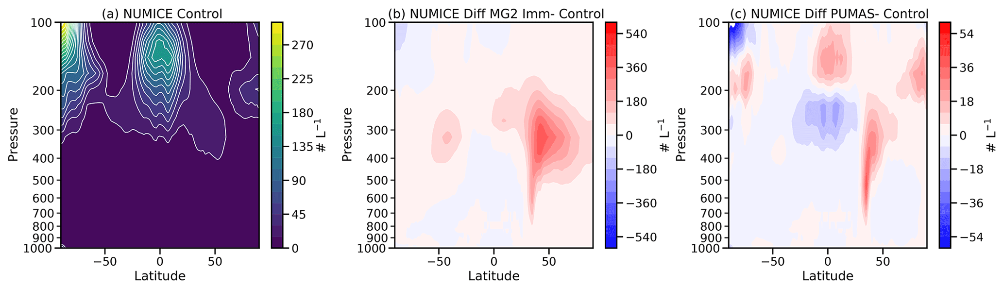
Figure 1 Zonal annual mean latitude height plots of the (a) cloud ice number (NUMICE) from the MG3 control simulation, (b) MG2 immersion freezing (no immersion limits in CNT dust) – control difference, and (c) PUMAS – control difference. Note the difference in scales between panels (b) and (c).

2.2.3 Vapor deposition onto snow

All versions of MG include vapor deposition onto ice in ice supersaturated conditions but not vapor deposition onto snow. For physical consistency, we have now added in PUMAS vapor deposition onto snow, for both the mass- and number-mixing ratios. This follows the same method as for vapor deposition onto cloud ice, as described in Morrison and Gettelman (2008, see their Eqs. 21 and 22), but uses snow size distribution parameters instead. Grid mean temperature, humidity, and snow mass-mixing ratio are used in the calculation. The calculation is limited to prevent the over-depletion of ice supersaturation (conditions cannot become ice-sub-saturated from vapor deposition).

2.2.4 Precipitation fall speed

In the MG1, MG2, and MG3 parameterizations, the sedimentation of all cloud and precipitation categories is sub-stepped to maintain the numerical stability for the explicit first-order upwind calculation. Precipitation has zero fall speed if it hits a level with no precipitation during a sedimentation sub-step. This will result in the stalling of the precipitation for the remainder of the full (not sub-stepped) time step. This can be a problem with long time steps (the standard CESM2 physics time step is 1800 s). We have implemented a correction which sets the number- and mass-weighted fall speeds for each hydrometeor category to that at the lowest level that contains non-zero (mass-mixing ratio with respect to dry air larger than 10⁻¹⁰) mass of that category before the sub-stepping and sedimentation calculation. Thus, number and mass for that category will fall at constant speeds below the lowest model level with non-zero category mass.

2.2.5 Implicit sedimentation

The default method used for sedimentation in all MG versions is an explicit first-order upwind calculation. Sedimentation sub-steps the time step to ensure numerical stability with the fall velocity. We have added an option for a time-implicit monotonic scheme for sedimentation using a single fall speed profile. The calculation is from Guo et al. (2021, their Appendix A). The number- and mass-mixing ratio q of a hydrometeor class at the n+1 time step and the k vertical layer ($q_k^{n+\mathrm{1}}$) are defined, as follows (Guo et al., 2021, Eq. A3):

$$\begin{array}{}\text{(2)}& q_k^{n+\mathrm{1}}={\displaystyle \frac{q_k^n\mathit{\delta }{z}_k+q_{k-\mathrm{1}}^{n+\mathrm{1}}{v}_{k-\mathrm{1}}\mathit{\delta }t}{\mathit{\delta }{z}_k+v_k\mathit{\delta }t}},\end{array}$$

where δt is time step, v_k is the number- or mass-weighted mean fall velocity at the kth vertical layer, and δz_k is the depth of the kth vertical layer. Note that k increases downward so that the flux is dependent on what is above, and the fall speed correction will have no or little impact. The implicit scheme was originally derived from the GFDL microphysics (see the appendices in Harris et al., 2020, and Zhou et al., 2019) and reduces sensitivity to the time step without sub-stepping (see Sect. 4.2). This approach is less accurate (more diffusive) at the gain of being much faster, as shown by Guo et al. (2021). In Sect. 4.2, we will show that it does not introduce significant errors in the solutions.

2.2.6 Modification of accretion

The autoconversion parameterization in MG and PUMAS is from Khairoutdinov and Kogan (2000, KK2000). The KK2000 autoconversion to rain tendency ($\mathrm{\Delta }{q}_{\mathrm{r}}=-\mathrm{\Delta }{q}_{\mathrm{c}}$), the change in mass-mixing ratio per second, is defined as follows:

$$\begin{array}{}\text{(3)}& \mathrm{\Delta }{q}_{\mathrm{r}\text{AUTO}}=A{q}_{\mathrm{c}}^B{n}_{\mathrm{c}}^C,\end{array}$$

where A=13.5, B=2.74, and $C=-\mathrm{1.1}$. Accretion (an additional Δq_r) is defined as follows:

$$\begin{array}{}\text{(4)}& \mathrm{\Delta }{q}_{\mathrm{r}\text{ACCRE}}=A(q_{\mathrm{c}}{q}_{\mathrm{r}}{)}^B,\end{array}$$

where A=67, and B=1.15. In principle, if there is autoconversion in a long time step, then the autoconverted rain (q_r) may accrete cloud liquid. This change may impact aerosol–cloud interactions by allowing accretion to operate on the newly autoconverted rain, by adding it to the existing rain mass for the calculation of accretion, so that it becomes the following:

$$\begin{array}{}\text{(5)}& \mathrm{\Delta }{q}_{\mathrm{r}\text{ACCRE}}=A\left(\right[q_{\mathrm{c}}-\mathrm{\Delta }{q}_{\mathrm{r}\text{AUTO}}\left]\right[q_{\mathrm{r}}+\mathrm{\Delta }{q}_{\mathrm{r}\text{AUTO}}]{)}^B.\end{array}$$

This allows accretion to occur during the same time step as the initial rain formation from autoconversion. We hypothesize that this may increase the accretion to autoconversion ratio and that it might impact the indirect aerosol forcing (Gettelman, 2015).

2.2.7 GPU directives

The atmosphere model consists of many parameterizations whose calculations are either grid independent or column independent. Therefore, it is possible to achieve massive parallelism for a parameterization by carefully restructuring the code and increasing the number of columns (for a global model, this means increasing the horizontal resolution), which then becomes a natural fit for GPU computing (Sun et al., 2018).

In this study, the PUMAS code is GPU-enabled by using the OpenACC directives, which allows the same source code to run on either the CPU or GPU and keep its maintainability. The test machines used in this paper are Cheyenne (https://www2.cisl.ucar.edu/resources/computational-systems/cheyenne, last access: 14 March 2023) and Casper (https://www2.cisl.ucar.edu/resources/computational-systems/casper, last access: 14 March 2023) at the National Center for Atmospheric Research (NCAR). Cheyenne is a homogeneous cluster with CPU-based nodes only, while Casper is a heterogeneous cluster with the NVIDIA V100 GPUs available on some computed nodes. The performance comparison below is made between one full CPU node on Cheyenne or Casper (i.e., 36 CPU cores) and one V100 GPU on Casper. We limit the simulation length to 1 d, which we find is long enough to show the performance difference. We mainly measure the timing information of the calculations within PUMAS and report the maximum wall clock time among the Message Passing Interface (MPI) processes that are averaged over the simulation length and sub-cycles (there are, by default, three sub-steps per time step for the calculation of the MG2 tendency using the 1^∘ resolution). For the GPU simulation, we also measure the timing information of the GPU computations and data copy between the CPU (i.e., host), GPU (i.e., device), and GPU internal memory allocation to better illustrate their relative computational cost. Last, but not the least, we vary the parameter “PCOLS” maximum number of atmospheric columns per single processing element (called a chunk). As noted by Worley and Drake (2005), there can be multiple chunks per MPI process. PCOLS is varied from 16 (the default value) to 1536 (the theoretical maximum number for 1^∘ resolution and 36 MPI processes) to reveal its impact on the CPU and GPU performance.

Figure 2 shows the computational time of the CPU and GPU for PUMAS without graupel. The figure compares computational times with increasing values of PCOLS. The newer Intel Skylake processors on Casper slightly outperform the previous generation of Intel Broadwell processors on Cheyenne. In addition, the CPU runs consistently show longer computational time with respect to increased PCOLS, which is likely a penalty caused by lack of cache for a larger chunk size. In contrast, the GPU run is significantly slower than the CPU run when PCOLS=16, and more than half of the time is spent on the computation (shown by pink bars). When PCOLS increases, more data are copied from CPU to GPU each time, meaning a higher parallelism and fewer total kernel launches on the GPU, as well as less frequent data movement between CPU and GPU. All of these factors contribute to the rapid decrease in computational time for the GPU run with larger PCOLS. A factor of 2× to 3× total speedup for the GPU relative to CPU is observed when PCOLS=1536. This suggests that we should expect to benefit from GPU computing only when our problem size (i.e., number of columns per GPU) is large enough. We also notice that the data movement could be more costly than computation for a smaller chunk size. Porting additional CAM physics parameterizations that use the same data to the GPU would likely reduce the relative cost of data movement and result in even more effective speedups. Even at PCOLS=1536, the data transfer time is larger than the total computation time in Fig. 2.

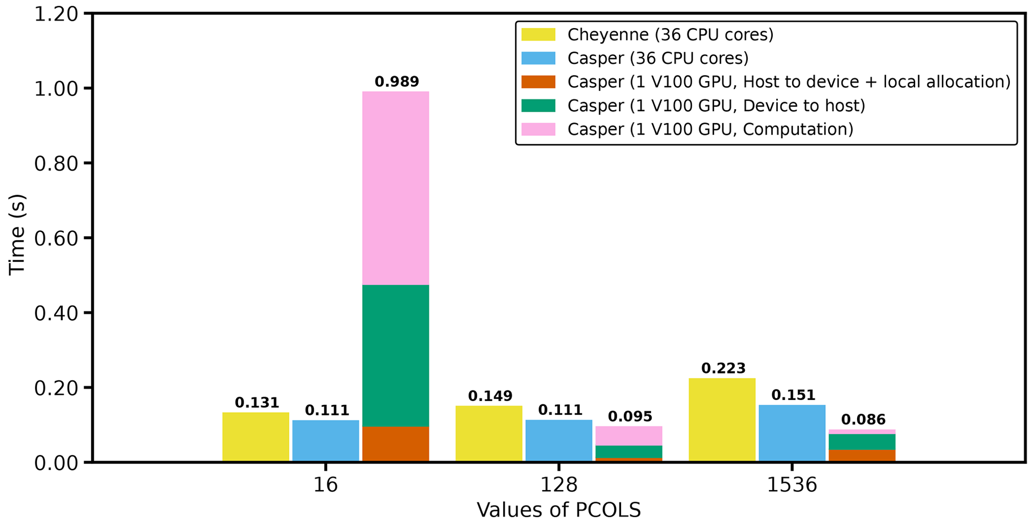
Figure 2 Averaged GPU-enabled MG2 runtime per sub-step for different configurations on the CPU and GPU. The computational time on GPUs is further divided into the time spent copying data from the host to the device, from the device back to host, and time spent in pure computation. Simulations are performed on the Cheyenne and Casper computer systems, with details described in Sect. 2.2.7.

The encouraging results here serve as a proof of concept for porting PUMAS to GPU. A separate paper has been submitted (Sun et al., 2022) to describe the technical details of porting PUMAS to GPU, optimizing the implementation, and evaluating the CPU and GPU performance with different configurations.

The addition of OpenACC directives is included in all the PUMAS tests but does not change the scientific results, as it results in only round off-level changes.

2.2.8 Additional switches

An additional series of options were added to the PUMAS scheme to adjust the fall speed, evaporation rate of cloud liquid and sedimenting condensate, and ability to use different ice nucleation options. The changes enhance portability and enable the PUMAS code to run in the ECMWF IFS system. This code is currently available in the PUMAS GitHub repository but detailed in other work.

3 Methodology

Our analysis looks at the impact of the changes described in Sect. 2 on the mean state, present-day climate, in addition to the implications for climate forcing and climate feedbacks. Cloud microphysics impacts the forcing of climate via interactions with aerosol particles in the atmosphere that change cloud condensation nuclei (CCN), as first noted by Twomey (1977). This has significant possible feedbacks on cloud drops and radiation, as recently reviewed by Bellouin et al. (2020). Cloud microphysical responses to increased CCN and ice nucleus (IN) concentrations are a critical forcing agent for climate. Furthermore, clouds respond to the environmental state when the planet warms due to other factors (such as the increase in anthropogenic greenhouse gases). These cloud feedbacks are the largest uncertainty in determining the climate sensitivity, which is the response of the climate system to an imposed forcing (e.g., Gettelman et al., 2016; Zelinka et al., 2020; Sherwood et al., 2020). We assess how both aerosol forcing and climate feedbacks change due to changes in the cloud microphysics with detailed simulations and analysis.

3.1 Simulations

We conduct several 6-year-long simulations using near-present-day cyclic boundary conditions for the year 2000. Boundary conditions used to force the model are climatological monthly averages over 1995–2000, including greenhouse gases, atmospheric oxidants, and emissions of aerosols. The climatological annual cycle is repeated each year. We also use averaged sea surface temperatures (SSTs) from observations (Hurrell et al., 2010). Data are compiled monthly and smoothly interpolated between months. Model resolution for CAM6 is 0.9^∘ latitude $\times \mathrm{1.25}{}^{\circ }$ longitude, with 32 levels in the vertical up to 10 hPa, a standard physics time step of 1800 s, and three coupling periods between microphysics and cloud macrophysics (turbulence and large-scale condensation), for a default microphysics time step of 600 s. A total of 6 years is sufficient so that the differences between past, present, and future configurations (see below) are much larger than the interannual standard deviation of global quantities (e.g., the signals are larger than the internal variability).

For each of the cases described below in Sect. 3.2, we conduct the following experiments. The first is a simulation with present-day (PD; year 2000) boundary conditions including SSTs, greenhouse gases (GHGs), and aerosol emissions. Next, we conduct simulations with (a) 1850 estimated aerosol emissions, termed preindustrial (PI), and (b) SSTs increased uniformly by +4 K (SST4K). All other boundary conditions (especially GHGs) are the same. When compared with the PD simulation, the PI assesses the impact of aerosol forcing, and SST4K assesses the impact of cloud feedbacks, which are representative of the full model response to warming, as first noted by Cess et al. (1989) and verified for CESM2 by Gettelman et al. (2019b).

For a detailed analysis, we also conduct single-column model simulations with the Single Column Atmosphere Model (SCAM) that is available as a part of CAM (Gettelman et al., 2019c). SCAM runs exactly the same atmospheric physics parameterization code as the full 3D simulations. We focus on the Atmospheric Radiation Measurement (ARM) program case from June 1997 for a month over the Central Great Plains (Oklahoma, USA), called the ARM97 case, in addition to the Mixed-Phase Arctic Cloud Experiment (M-PACE) case from October 2004 over the North Slope Borough of Alaska. The cases are detailed in Gettelman et al. (2019c). The standard time step in SCAM is 1200 s, with four microphysics sub-steps for a microphysics time step of 300 s.

3.2 Description of sensitivity tests

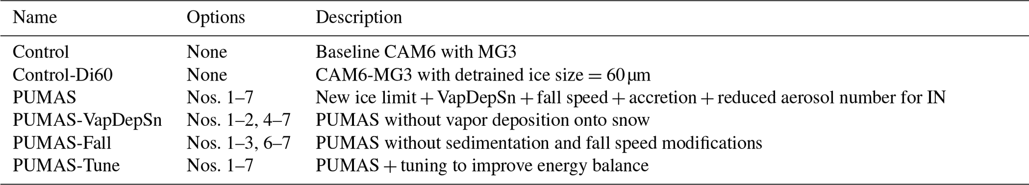
Sensitivity tests are grouped sequentially, as indicated in Table 1, with the testing many of the items listed in Sect. 2.2 and with the item numbers also listed in that section. The first is a control case, using the standard CAM6 and the MG3 microphysics. All of these tests include graupel. Next, we test a PUMAS case with modifications nos. 1–7 listed in Sect. 2.2, except for no. 8 (optional switches to replicate processes in the ECMWF IFS). This includes (1) refactoring the ice number limiter, (2) using a reduced aerosol number for ice nucleation, (3) allowing the vapor depositional growth of snow, (4) applying fall speed corrections, (5) noting implicit sedimentation, (6) seeing newly autoconverted rain with accretion, and (7) adding ACC directives. An additional modification is to increase the specified diameter of ice crystals detrained from deep convection (from 25 to 60 µm; Control-Di60). We test the impact of this change in a separate simulation based on the control case. The PUMAS simulation in which we use the CNT immersion freezing without a reduced aerosol number to act as INPs (no. 2) is illustrated in Fig. 1 (PUMAS-Imm). We then look at the impact of removing vapor deposition onto snow (no. 3) in PUMAS, as described in Sect. 2.2 (PUMAS-VapDepSn). Next, we test removing the fall speed modifications (no. 4) and implicit sedimentation (no. 5) in PUMAS simulations in the PUMAS-Fall simulations. Because the fall speed modifications mainly impact the explicit rather than implicit treatment of sedimentation, we also tested the fall speed modifications along with the explicit sedimentation in PUMAS (e.g., testing explicit sedimentation with the fall speed correction). The results are basically the same as for the explicit sedimentation without the fall speed correction in PUMAS-Fall (not shown), indicating that the fall speed correction has little impact. Finally, we also explore a simulation in which we adjust (tune) uncertain microphysical parameters to increase cloud water and ice to come close to the control case (PUMAS-Tune). This tuning is accomplished by scaling the autoconversion of cloud to rain by a factor of 0.5 from the control case and increasing the threshold diameter for ice autoconversion to 1000 µm (from the control value of 500 µm).

Table 1 Description of the simulations. Numbers in the options column correspond to the changes listed in Sect. 2.2.

4 Results

4.1 Process rates

To look in detail at the effects of changes to the microphysics scheme, we focus on SCAM simulations for the ARM97 summer case. Figure 3 illustrates liquid (Fig. 3a–c), ice (Fig. 3d–f), rain (Fig. 3g–i), and snow (Fig. 3j–l) process rates. Graupel was included in these simulations but is not shown and discussed briefly below. Figure 3a, d, g, and j (left column) are the control simulation, the center column (Fig. 3b, e, h, k) is the PUMAS modified code (changes nos. 1–7 from Sect. 2.2), and the right column (Fig. 3c, f, i, l) is the difference between the two. Differences in liquid at pressures less than 600 hPa mainly come from changes in ice and mixed-phase processes (vapor deposition). In particular, there is less accretion of liquid onto snow (blue dotted–dashed line) and vapor deposition onto snow (Bergeron snow; solid teal line), reducing the liquid loss rates at higher altitudes. At lower altitudes (pressures >600 hPa), there are small changes to liquid, with less liquid sedimentation (solid blue line) and more loss from the accretion of cloud by rain (accretion; dashed turquoise line).

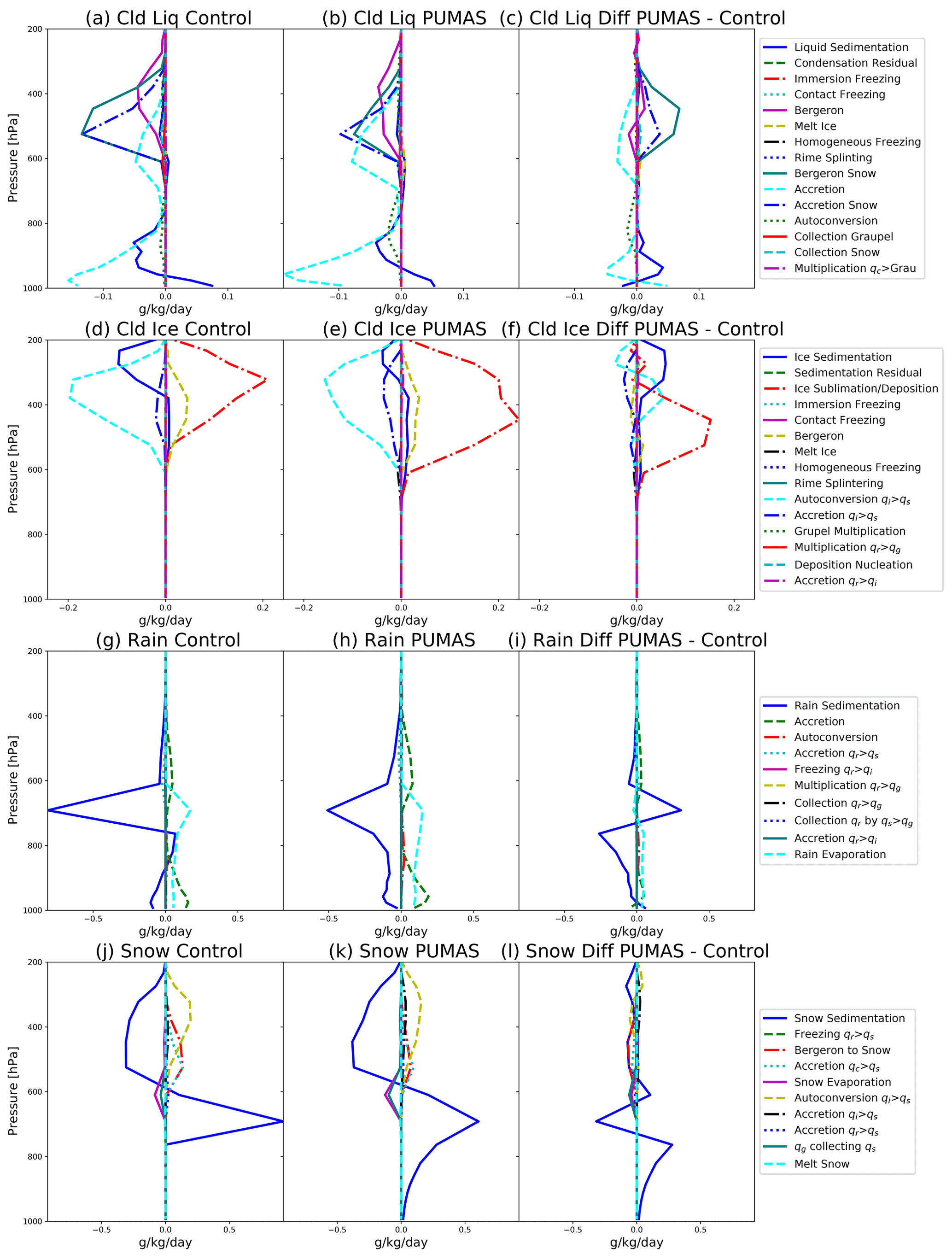
Figure 3 Mass-mixing-ratio process rate profiles from SCAM simulations. The left column (a, d, g, j) is the MG3 control simulation, the center column (b, e, h, k) is the PUMAS code (Table 1; change nos. 1–7), and the right column (c, f, i, l) is the difference. The top row (a–c) shows results for cloud liquid, cloud ice (d–f), rain (g–i), and snow (j–l), respectively.

Ice microphysics sees larger changes, with a decrease in ice mass loss from sedimentation (solid blue line), leading to a positive net change. This is caused by a larger ice number that comes from removing the NIMAX limiter and results in more ice mass. Cloud ice remaining longer in the atmosphere increases the availability for sublimation and deposition (dotted–dashed red line) as well.

Precipitation changes in Fig. 3 are also significant. Rain has a negative sedimentation tendency (solid blue line) all the way to the surface in the revised code (Fig. 3h), with reduced fall speeds higher up. Snow has a positive sedimentation tendency (solid blue line) from 800–600 hPa, as snow falling from above enters a layer below. In PUMAS, this continues all the way to the surface (Fig. 3k) because the nonzero fall speed was added below the lowest level of precipitation. The implicit sedimentation does not seem to introduce any numerical issues with rain or snow.

Graupel changes (not shown) do not significantly affect snow or other hydrometeors and come mostly from differences in the graupel-collecting snow term (dashed turquoise line), which is larger (more negative) in PUMAS (Fig. 3l).

We have explored in detail how the different parts of the PUMAS code create these differences, by plotting some of the changes separately (not shown). The upper-level increases in cloud ice deposition and sublimation come from the ice number limiter change. The limiter also reduces the low-level accretion of cloud liquid (q_c) to rain (q_r) and snow (q_s). The implicit sedimentation results in more accretion of cloud liquid. The new accretion increases the accretion of cloud liquid as well but reduces cloud ice deposition/sublimation. Thus, not all the changes act in the same way. The changes due to the accretion, including the newly autoconverted rain, have a smaller impact (limited to increasing low-level accretion) than the explicit sedimentation or ice limiter changes.

4.2 Time step sensitivity

We have also used the SCAM cases as a way to explore the time step sensitivity of the schemes. To focus on the microphysics, we set a 1200 s physics time step in SCAM, with four sub-steps for the CLUBB-unified turbulence scheme. We then can sub-step the microphysics within the 300 s sub-step. This takes the same condensation from turbulence and passes it to the microphysics, which we run from 300 to 10 s (e.g., 1 to 30 microphysics sub-steps). The results are illustrated in Fig. 4 for the June 1997 (ARM97) case. We focus on the control case (MG3), all the PUMAS modifications (PUMAS), and the PUMAS without the implicit sedimentation and fall speed corrections (PUMAS-Fall). Other sensitivity cases are similar to PUMAS. Figure 5 illustrates the same tests but for the Mixed-Phase Arctic Cloud Experiment (M-PACE) in October 2004 over the North Slope Borough of Alaska.

Figure 4 Time-averaged SCAM profiles from the ARM97 case with different time steps, as indicated in the legend. MG3 control cases (blue), PUMAS-Fall (orange), and PUMAS (red) are shown. Simulation names are defined in Table 1. Results are shown for (a) cloud liquid, (b) cloud ice, (c) supercooled liquid, (d) rain, and (e) snow mass-mixing ratios and (f) cloud fraction. Thicker lines indicate longer time steps.

Figure 5 As in Fig. 4 except for the M-PACE case.

Several results stand out. First, cloud liquid and rain (Fig. 4a and d) are fairly sensitive to time step changes for the SCAM ARM97 case in the control (MG3) configuration. The same is true for supercooled liquid (Fig. 4c). The PUMAS code reduces the time step sensitivity of most of the hydrometeors. This is particularly true for the M-PACE case in Fig. 5, where cloud (Fig. 5a), supercooled liquid (Fig. 5c), and cloud ice (Fig. 5b) have much less variability across time steps than in the control MG3 case. Most of this improvement is not seen if the fall speed and sedimentation changes are removed, indicating that implicit sedimentation contributes substantially to the reduced sensitivity of solutions to time step (as expected). Figure 4b and c indicate reductions in supercooled liquid water and ice with the microphysical changes in PUMAS.

Impacts of the implicit sedimentation and fall speed changes are seen in the rain mass (Fig. 4d). The peak rain mass for PUMAS in the ARM97 case is less variable in PUMAS than in the control or in PUMAS without implicit sedimentation. However, there is a reduced gradient below the peak for PUMAS, which may be caused by the more diffusive nature of the formulation. This is not an issue in the M-PACE case (Fig. 5d). It is not seen to be a problem in the 3D simulations.

The M-PACE case (Fig. 5) has less sensitivity to the time step than ARM97 for the control MG3 case and even less sensitivity for PUMAS. Reduced sensitivity in all cases may have to do with the absence of deep convective cloud and deeper cloud in the M-PACE, while such cloud is present throughout the column in ARM97. Cloud liquid (all supercooled; Fig. 5a and c) has little sensitivity in PUMAS, less than with MG3 or PUMAS-Fall, again indicating the importance of implicit sedimentation. There is less cloud ice (Fig. 5b) but more snow in the PUMAS simulations compared to MG3. Overall, besides the reduced time step sensitivity, PUMAS and PUMAS-Fall give similar results for these SCAM cases.

4.3 Mean state climate

Figure 6 illustrates the zonal mean climatologies from 6-year global simulations of CAM6 with control microphysics (MG3) and updated PUMAS code. Also shown are observations of the radiative fluxes and clouds from the CERES (Clouds and the Earth's Radiant Energy System) satellite Energy Balanced and Filled (EBAF) products (Loeb et al., 2018), liquid water path (LWP) from the CERES SYN product (Rutan et al., 2015), and precipitation from the Global Precipitation Climatology Project (GPCP; Adler et al., 2018). We test the code following the experiments in Table 1. PUMAS (blue) is the full set of modifications. PUMAS-VapDepSn (orange) removes the vapor deposition onto snow, PUMAS-Fall (green) removes the fall speed changes and uses an explicit rather than implicit sedimentation calculation, and PUMAS-Tune (red) increases liquid and ice mass with parameter changes. The full PUMAS ice modifications (blue) reduce the overall cloud radiative effect (CRE) magnitude (less negative shortwave (SW) and less positive longwave (LW) effect) from the control MG3 case by about 2.5 W m⁻² (Fig. 6g and h). The difference tends to reduce SW biases but increase LW biases with respect to CERES. This is due to the lower LWP (Fig. 6a) and ice water path (IWP; Fig. 6b). Cloud fraction, cloud-top liquid number, and precipitation (Fig. 6c, d and f) are similar across all simulations. Note that the satellite data for LWP (Fig. 6a) and cloud fraction (Fig. 6c; based on CERES and MODIS clouds) are not reliable at high southern latitudes over the ice sheet. It is clear that the highest water contents are not over the South Pole. The PUMAS-Tune case is designed to increase liquid and ice (Fig. 6a and b) in order to increase the magnitude of the cloud radiative effects so that they are more similar to the control (Fig. 6g and h), but PUMAS-Tune also decreases the ice number (Fig. 6e). The resulting cloud radiative effects (Fig. 6g and h) are of a lower magnitude than CERES LW observations but generally within the variability in the observations (purple shading). Note that the change to detrained ice size (included in all PUMAS simulations) is tested on its own with the control model (Control-Di60), and it increases LWP (Fig. 6a) and decreases IWP (Fig. 6b), likely through the faster sedimentation of larger ice crystals. Also note that the revised immersion freezing (present in all the PUMAS simulations) have higher ice numbers (Fig. 6e) from 30–60^∘ N latitude.

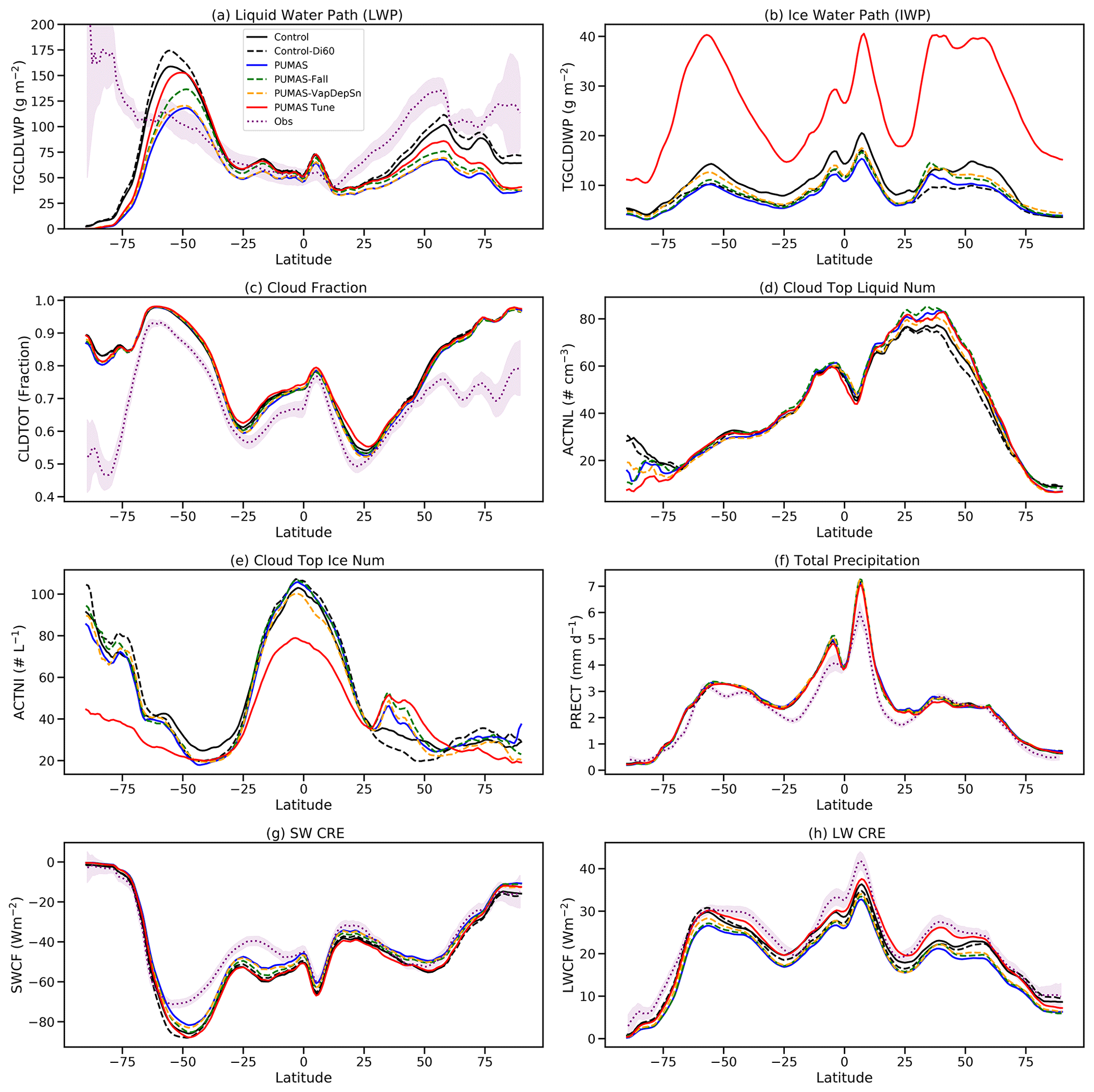
Figure 6 Zonal mean annual averages from 6-year global simulations for the MG3 control (black), PUMAS (blue), PUMAS-Fall (green), PUMAS-VapDepSn (orange), and PUMAS-Tune (red). Simulation names are defined in Table 1. Also shown is the CERES EBAF climatology (purple), with 1 standard deviation of the annual means. (a) Liquid water path (LWP). (b) Ice water path (IWP). (c) Cloud fraction. (d) Cloud-top liquid number. (e) Cloud-top drop number. (f) Total precipitation. (g) Shortwave (SW) cloud radiative effect (CRE). (h) Longwave (LW) CRE.

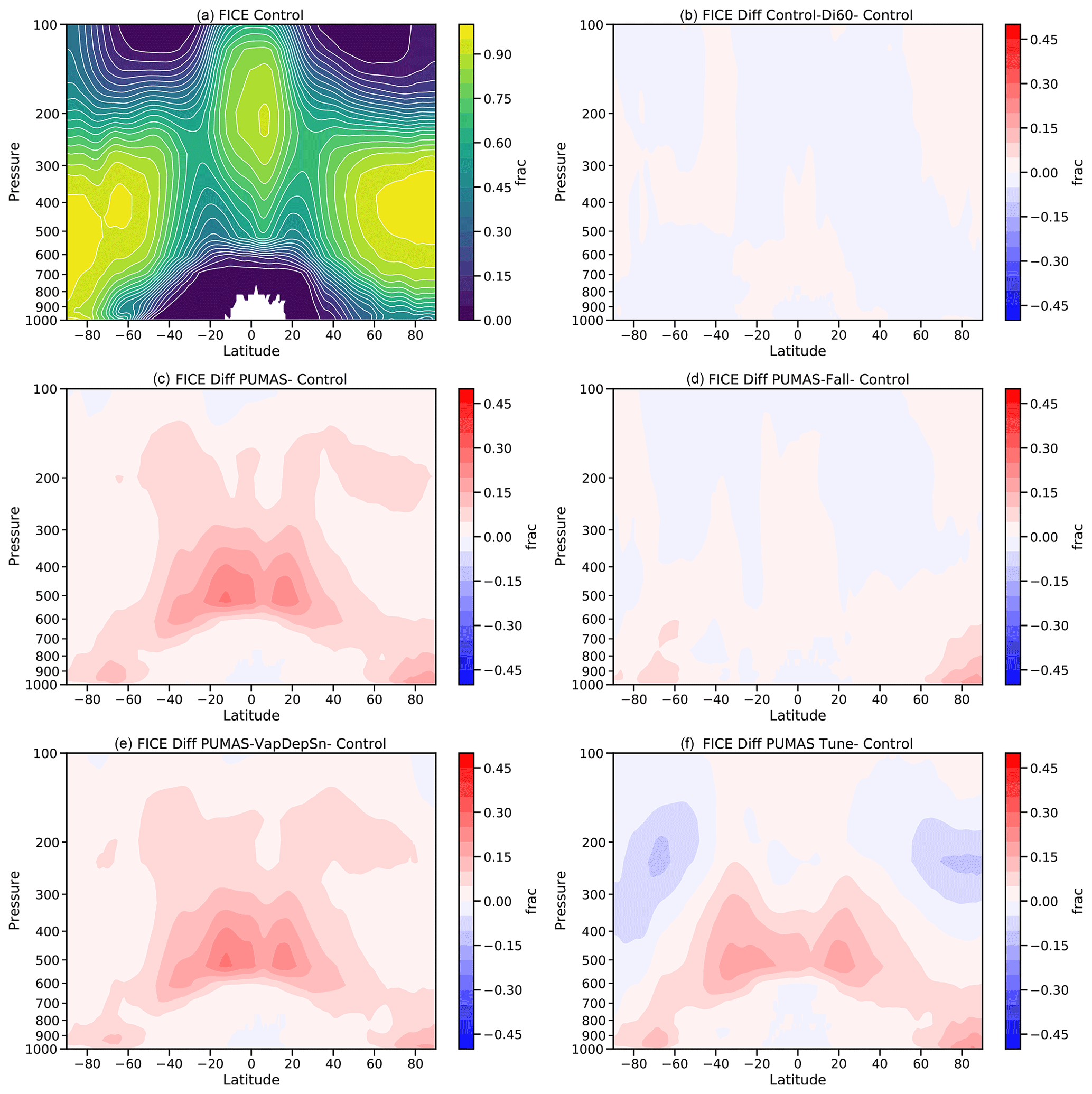
Figure 7 illustrates the ice fraction in the control and PUMAS simulations. The ice fraction is calculated at each location and time step as the ice mass-mixing ratio divided by the total cloud water (ice and liquid) mass-mixing ratio. An increase in ice fraction reduces the CRE from supercooled liquid water but increases CRE from ice. Cloud ice provides a negative cloud-phase feedback when it is reduced under climate warming. The detrained ice size change does not impact the ice fraction in the control simulation (Fig. 7b). PUMAS features an increase in the ice fraction in the tropical middle troposphere (600–300 hPa) relative to the MG3 control simulation (Fig. 7c). It appears that the implicit sedimentation change is the reason, as removing the implicit sedimentation and the fall speed correction (Fig. 7d) produces ice fractions that resemble the control case. Our tests showed that adding the fall speed correction to explicit sedimentation does not matter (not shown). The sedimentation likely impacts the evolution of ice near the freezing level. There are also some impacts at high latitudes. The tuning of clouds to increase liquid and ice water path modifies the ice fraction due to substantial differences in the liquid and ice water path (Fig. 6), generally resulting in more moderate changes to the ice fraction relative to the control than with the standard PUMAS (with less condensate mass; Fig. 7c).

Figure 7 Zonal annual mean ice fraction for the (a) control (MG3) and differences in ice fraction for (b) Control-Di60 – control, (c) PUMAS – control, (d) PUMAS-Fall – control, (e) PUMAS-VapDepSn – control, and (f) PUMAS-Tune – control. Simulation names are defined in Table 1.

4.4 Cloud feedback

Cloud feedback is determined using a kernel-adjusted cloud radiative forcing, as described by Soden et al. (2008) and implemented in CESM by Gettelman et al. (2012) (also used by Gettelman et al., 2019b).

Figure 8 illustrates the kernel-adjusted cloud feedback estimates, weighted by the cosine of latitude (so that the area under the curve is the contribution to the global mean). Table 2 presents the global averages. PUMAS slightly increases the cloud feedback, lowering the LW and increasing the SW. Some of this results from the change to the detrained ice size (Control-Di60) and not PUMAS itself. The PUMAS-Fall SW feedbacks are very close to the Control-Di60 case, indicating that the differences in SW feedbacks are perhaps due to the implicit sedimentation. The change to the fall speed was tested with explicit sedimentation and does not impact feedbacks. The mechanism might be through the changes to the ice phase seen in Fig. 7. The net cloud feedback (Fig. 8c) is reduced from 30–70^∘ latitude in both hemispheres but offset with changes at higher latitudes. The PUMAS-Tune simulation with enhanced cloud water has larger SW cloud feedbacks, from 30^∘ S–30^∘ N, but there was some offsetting of lower LW feedbacks. This is likely due to the significantly larger ice mass changing high (cirrus) cloud feedbacks, as LW feedbacks are lower in the tropics in regions of higher ice mass and number, from 20–40^∘ N (Fig. 6).

Figure 8 Zonal mean cloud feedback from SST4K simulations, with the control (black), Control-Di60 (black dashed), PUMAS (blue), PUMAS-Tune (red), PUMAS-VapDepSn (orange dash), and PUMAS-Fall (green dash) shown. Simulation names are defined in Table 1. Feedbacks use kernel-adjusted cloud radiative effects, as described in Gettelman et al. (2013) and Gettelman et al. (2019b). Results are shown for (a) SW cloud feedback, (b) LW cloud feedback, and (c) net (LW+SW) cloud feedback.

Table 2 Global average kernel-adjusted cloud feedback (CF; $\mathrm{W}{\mathrm{m}}^{-\mathrm{2}}{\mathrm{K}}^{-\mathrm{1}}$).

We have examined maps of cloud feedback by regime for the LW and SW feedbacks, and there do not appear to be large and significant systematic differences in cloud feedback between the control and PUMAS simulations. On the whole, the impact of PUMAS on cloud feedbacks is moderate and not significant.

4.5 Aerosol forcing

Finally, we assess the impact of the changes in cloud microphysics on the aerosol forcing of climate by running 6-year simulations identical to the present-day (PD) simulations but with the aerosol emissions set to 1850 emissions, i.e., the preindustrial (PI) era. The difference in PD–PI represents the impact of aerosols on climate. The indirect effect of aerosols on clouds is illustrated by the change in the cloud radiative effect (ΔCRE). For liquid clouds, this is mostly in the SW (ΔSWCRE), and for ice clouds, this is both the SW and LW (ΔLWCRE). The direct radiative effect of aerosols is the clear-sky shortwave flux change (ΔSW_clr). The total effect is the all-sky residual top-of-model (ΔRESTOM) flux change. Changes in the column drop number (ΔCDNC) and liquid water path (ΔLWP) and ice water path (ΔIWP) are also assessed, which drive changes in CRE for clouds with liquid. For all quantities, the global average PD–PI differences are larger than twice the interannual standard deviation of global means of these quantities.

The CAM6 total radiative effect due to aerosols (ΔRESTOM) is on the high end of the range assessed by Bellouin et al. (2020). Overall, the net aerosol forcing in the present day (PD–PI) defined by ΔRESTOM drops by less than 10 % with the PUMAS modifications (Table 3). This occurs due to small reductions in the negative SW clear-sky forcing (direct effects of aerosols) and small reductions in the SW cloud radiative effect changes but is partially offset by reductions in the positive LW forcing as well. Thus, the magnitude of the components is slightly reduced. The PD–PI percent change in LWP is lower with PUMAS than the control (Table 3). The cloud drop number increases by 30 %, while the cloud fraction increases by less than 1 %. The simulations are similar for the different sensitivity tests, but this masks regional differences.

Table 3 Global average forcing change due to the aerosol of PD–PI (W m⁻²).

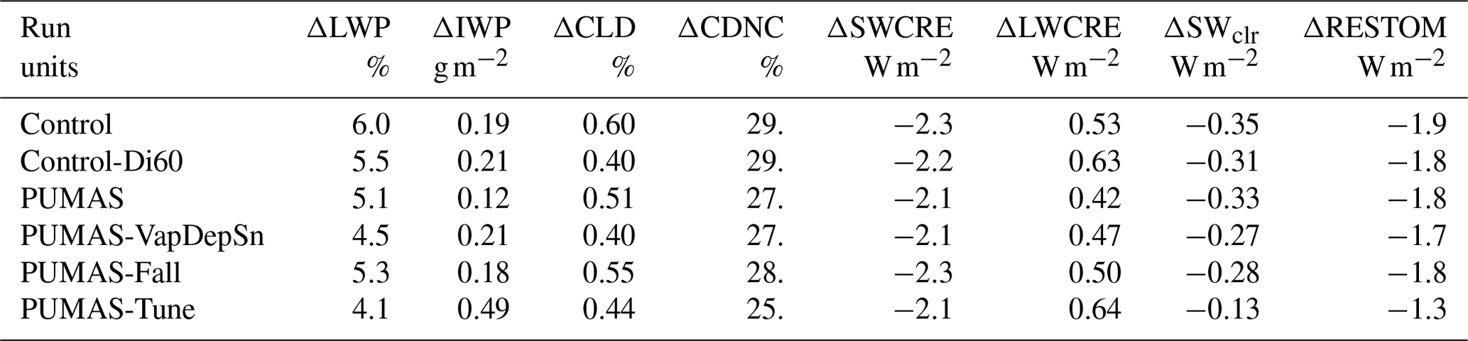
Figure 9 illustrates the zonal mean changes in key quantities between pairs of PD and PI simulations. The gross aerosol forcing of climate in the SW (Fig. 9a) and LW (Fig. 9b) is similar in most of the PUMAS simulations compared to the control, where SW forcing is negative and becomes less so in the Northern Hemisphere. LW forcing is reduced in all three PUMAS configurations and the PUMAS-Tune simulation. The residual net change in the top-of-model (TOM) flux (Fig. 9c) has a lower magnitude (less negative) than the control in Northern Hemisphere high latitudes for the PUMAS-Tune simulations (Fig. 9c). There is a significant reduction in the LWP and column cloud drop number (CDNUMC) response from 25–90^∘ N latitude (Fig. 9d and f), which drives the reductions in the magnitude of the SW CRE changes (Fig. 9a). Some of the difference is due to the smaller mean values. The percent change in LWP is reduced in PUMAS simulations (Table 3), but the percent change in drop number is similar, except for the PUMAS-Tune simulation.

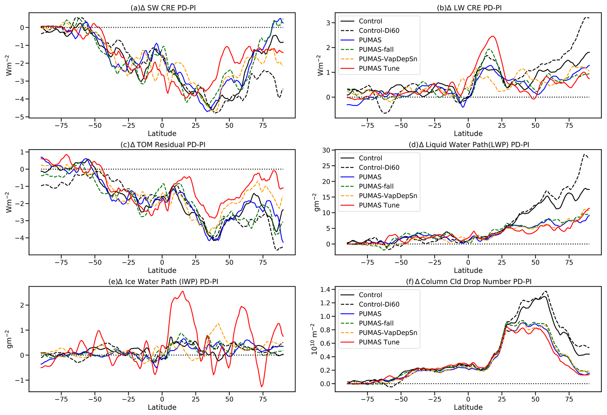
Figure 9 Zonal mean differences between control (PD) and 1850 aerosol (PI) simulations for four pairs of runs, i.e., control (black), Control-Di60 (black dash), PUMAS (blue), PUMAS-Fall (green dash), PUMAS-VapDepSn (orange dash), and PUMAS-Tune (red). Simulation names are defined in Table 1. Results are shown for the (a) change in SW CRE, (b) change in LW CRE, (c) change in net top-of-model flux (RESTOM), (d) change in LWP, (e) change in IWP, and (f) change in the column drop number.

Since the forcing response of most of the PUMAS simulations is similar, Fig. 10 compares maps of the patterns of differences (PD–PI) for the control (left column) and PUMAS (right column) simulations. Maps of the pattern of differences in Fig. 10 show that these changes occur in most places across the globe. SW CRE changes (Fig. 10a and b) are reduced with PUMAS slightly throughout the Northern Hemisphere and even into the Southern Hemisphere. There are some positive values over northeastern Asia. Changes are similar over the Pacific, with large impacts in the eastern Pacific that are a common feature of CAM aerosol–cloud interaction (ACI) effects but lower in PUMAS. The LW CRE changes (Fig. 10c and d) have more positive values (Fig. 10d) than the control simulation (Fig. 10c), especially over the Indian Ocean, which shifted from the eastern Pacific, with little net effect. The LWP changes (Fig. 10g and h) are smaller with PUMAS and localized closer to the source regions compared to the control. This is true especially in the Arctic (Fig. 10h). Some of this is due to lower mean values, but the percent change in LWP is smaller (Table 3), and the high-latitude LWP is reduced in PUMAS (Fig. 6a).

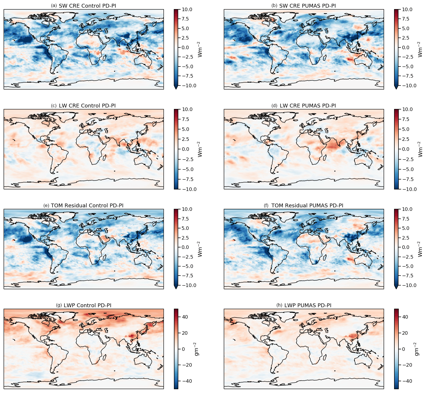
Figure 10 Differences between present-day (PD) and 1850 aerosol (PI) simulations for control (a, c, e, g) and PUMAS (b, d, f, h). Variables shown are the (a, b) SW cloud radiative effect (SW CRE), (c, d) LW cloud radiative effect (LW CRE), (e, f) RESTOM balance, and (g, h) liquid water path (LWP).

5 Discussion and summary

We have described several adjustments to the MG3 cloud microphysical scheme now renamed PUMAS, including refactoring of an ice number limiter, adjustments to the fall speed calculation and use of an implicit numerical method for sedimentation, the addition of a process (vapor deposition onto snow), and the adjustment of accretion and the aerosol numbers input to the immersion freezing calculation.

The vapor deposition onto the snow process has no significant effect on the simulations and neither does the fall speed correction, even with explicit sedimentation (we do not expect much impact with implicit sedimentation). The major impact on the simulations comes from the refactoring of the ice number limiter (NIMAX), ice nucleation, and the implicit sedimentation.

The following is a summary of the main results.

1. GPU-enabled microphysics code is significantly faster than the CPU version if a large number of columns can be loaded onto GPU accelerator chips. This results in a 2× to 3× speedup, with even more possibility for speedup at higher column counts. This would facilitate running at a higher horizontal resolution.

2. The refactoring of the ice number limiter (change 1) results in extremely high ice numbers due to the CNT formulation of immersion freezing in CAM6. This significant increase in ice number is anomalous and creates a different climate state. This necessitated adjusting the aerosol numbers and dust, in particular, used in immersion freezing (change 2). This might affect the solutions of Zhu et al. (2022), who removed the ice number limiter but used a smaller microphysical time step to control the unrealistic growth of ice number. One important message is that ice nucleation can have important climate effects.

3. The new PUMAS code reduces overall LWP and IWP. It is not clear what processes may be responsible for this, as it occurs in all PUMAS simulations. The increase in accretion might be partially responsible, in addition to the increased sedimentation limiting evaporation. The code can be adjusted to keep a more condensed water path by reducing the loss rates for liquid and ice, as performed in the PUMAS-Tune experiment.

4. The new PUMAS code reduces the aerosol-forcing magnitudes slightly, with offsetting effects on the total ACI. The mechanism may be related to higher ice numbers and less liquid water at high latitudes. There is little net change in the aerosol forcing but reductions in magnitude of SW and LW components.

5. The PUMAS changes have small impacts on cloud feedbacks and climate sensitivity. There are reductions in the Northern Hemisphere midlatitude feedbacks and increases in the Southern Hemisphere midlatitudes. Tropical feedbacks increase slightly. Mainly, feedback changes appear to be due to the implicit sedimentation (change 5); reverting this change makes PUMAS look more like the control.

6. The implicit sedimentation calculation (change 5) also contributes to lowering the aerosol forcing, likely through changes to precipitation production, with less change to LWP. The implicit sedimentation reduces sensitivity to the time step and increases the ice fraction near the freezing level. There does not seem to be an appreciable difference in the time-averaged precipitation or the precipitation process rates due to use of a less-accurate implicit method.

The next steps for PUMAS development include integrating the unified ice formulation of Eidhammer et al. (2016), further investigations into ice nucleation and the budget of INPs, and the exploration of a flexible form to the size distributions (Morrison et al., 2020). In addition, the GPU results motivate further work to add GPU directives to all the physical parameterizations in CAM.