Strategies for conservative and non-conservative monotone remapping on the sphere

Monotonicity is an important property of remapping operators for coupled weather and climate models. However, it is often challenging to design highly accurate operators that avoid the generation of new extrema or keep a remapped field between physically prescribed bounds. To that end, this paper explores several traditional and novel approaches for both conservative and non-conservative monotone remapping on the sphere. The accuracy and effectiveness of these algorithms are evaluated in the context of several different real and idealized fields and meshes.

1 Introduction

An important operation in global climate models is the transferring, or remapping, of data between different component grids. For example, information needs to be exchanged at the interface between the atmosphere and ocean models, when both are typically defined on different grids. Atmospheric models often use icosahedral or cubed sphere grids, while ocean models have relied on unstructured meshes (Satoh et al., 2008; Taylor et al., 2007; Ringler et al., 2013). Remapping of data between grids whose structures differ greatly is a challenging and important problem, as doing so inaccurately can impact the stability of coupled simulations (Beljaars et al., 2017). There are other circumstances in which accurate remapping operators are important, such as post-processing and mesh refinement. In the former case, the grid on which a simulation is performed may not be ideal for carrying out analysis, and transferring data onto a structured mesh that is more amenable for analysis is often useful. In the latter case, grid nesting (Harris and Lin, 2014) and adaptive grids (Jablonowski et al., 2006; Skamarock and Klemp, 1993) have been used to resolve the complex multiscale nature of the atmosphere. Ensuring the accurate interpolation of data between the different component grids in these simulations is crucial to preserving the models' overall accuracy (Slingo et al., 2009; Mahadevan et al., 2020).

There are a number of desirable properties of remapping operators, in addition to accuracy. These properties include consistency, conservation, and monotonicity and correspond, respectively, to the mapping of the constant field to the constant field, preservation of total mass, and no generation of new extrema (Ullrich and Taylor, 2015). These properties are necessary for ensuring important physical consistency of model simulations. Some fields, like mass (which is usually stored as density), are required to be conserved, while others, like tracers or mixing ratios, are required to satisfy certain bounds following the remapping process. It is therefore imperative for schemes that remap these fields to preserve conservation and global monotonicity constraints so as not to introduce artificial sources of error (Kritsikis et al., 2017).

The main property of remapping schemes that we are concerned with in this paper is monotonicity. In the case of conservative remapping, monotonicity is often achieved by way of limiters (Barth and Jespersen, 1989). In the conservative case, we are interested in applying the “clip and assured sum” (CAAS) method, which acts as a post-processing filter operation on the remapped field (Bradley et al., 2019). In the non-conservative case, we are interested in linear monotone remapping operators that depend only on the mesh structures and can be computed once and then applied in an offline manner.

TempestRemap (Ullrich and Taylor, 2015; Ullrich et al., 2016) is a widely used package for generating conservative, consistent, and (optionally) monotone linear maps between arbitrary grids on the sphere, with data stored as volume averages (finite-volume method) or as coefficients of a finite-element expansion. Although conservative remapping is necessary for ensuring, for example, that fluxes at the ocean–atmosphere interface preserve global invariants, when remapping states or vectors it is often the case that monotonicity and accuracy are more important than conservation. Indeed, when mapping from a coarse grid to a fine grid, conservative and monotone schemes will appear blocky because each fine grid volume completely within a coarse grid volume must exactly preserve the state of the coarse grid volume. Consequently, the Energy Exascale Earth System Model (Golaz et al., 2019, E3SM), which uses TempestRemap maps under the hood, falls back on bilinear maps for transferring state data when mapping from coarse-resolution to fine-resolution grids. To support the operational remapping of data in this manner, the methods developed in this paper have been implemented in v2.1.6 of the TempestRemap package (Ullrich et al., 2022).

This paper consists of three main sections. First, we will describe the basic setup of remapping problems, the test cases that are used in our numerical experiments, and the metrics used to assess the accuracy of the remapping schemes. In the next section, we will look at monotone conservative remapping. In general, it is difficult to construct remapping operators that satisfy conservation and monotonicity, while still maintaining high-order accuracy. So one of the main purposes of this section is to examine the extent to which a conservative and monotone remapping operator can maintain the accuracy of its non-monotone counterpart. We will also analyze the effectiveness of this conservative and monotone operator in minimizing the errors associated with the remapping of discontinuous source fields, as well its ability to remap real data fields accurately. The subject of the next section is non-conservative monotone remapping, and it is divided into two main parts. The first part focuses on traditional approaches to monotone remapping and includes a description of the bilinear method used in the Earth System Modeling Framework (ESMF) (Hill et al., 2004), as well as two additional approaches that may provide advantages in some circumstances. In the second part, we show that the accuracy of these traditional approaches is reduced when remapping from source meshes that are finer than the target mesh, and a method is introduced to correct this. We end with conclusions and future research directions.

2 Preliminaries

Let Ω denote the unit sphere. Given a source mesh, Ω^s, and a target mesh, Ω^t, the remapping operator, R, is a matrix constructed to satisfy

$$\begin{array}{}\text{(1)}& {\mathit{\psi }}^{\mathrm{t}}=\mathbf{R}{\mathit{\psi }}^{\mathrm{s}},\end{array}$$

where ${\mathit{\psi }}^{\mathrm{s}}=({\mathit{\psi }}_{\mathrm{1}}^{\mathrm{s}},\mathrm{\dots },{\mathit{\psi }}_{\mathrm{s}}^{f_{\mathrm{s}}})\in {\mathbb{R}}^{f_{\mathrm{s}}}$ and ${\mathit{\psi }}^{\mathrm{t}}=({\mathit{\psi }}_{\mathrm{1}}^{\mathrm{t}},\mathrm{\dots },{\mathit{\psi }}_{\mathrm{t}}^{f_{\mathrm{t}}})\in {\mathbb{R}}^{f_{\mathrm{t}}}$ are vectors of discrete density values on the source and target meshes, respectively. The number of degrees of freedom on the source mesh is denoted by f_s, and the number of degrees of freedom on the target mesh is denoted by f_t. Here, ψ^s corresponds to the discretization of a function $\mathit{\psi }:{\mathrm{\Omega }}^{\mathrm{s}}\to \mathbb{R}$, either by sampling ψ at a set of discrete nodes by pointwise sampling or over a set of regions by area averaging. The operators that discretize the function ψ into the discrete vectors ψ^s and ψ^t are denoted by D^s and D^t. Degrees of freedom on the source and target meshes can be stored in various ways, though in this paper we focus on finite-volume or finite-element methods. In the former case, degrees of freedom on the mesh correspond to area or volume averages, and in the latter, they are stored as coefficients of basis functions with compact support. For instance, for the spectral element method, a type of finite-element method, it is typical to store degrees of freedom at a set $N_p^{\mathrm{2}}$ Gauss–Lobatto–Legendre (GLL) nodes within each face.

Following Ullrich and Taylor (2015), the metrics that are used to assess the accuracy of the remapping schemes in this paper are as follows.

$$\begin{array}{}\text{(2)}& {\displaystyle }{L}_{\mathrm{1}}\equiv {\displaystyle \frac{I^{\mathrm{t}}\left[\right|{\mathbf{RD}}^{\mathrm{s}}\left(\mathit{\psi }\right)-{\mathbf{D}}^{\mathrm{t}}\left(\mathit{\psi }\right)\left|\right]}{I^{\mathrm{t}}\left[\right|{\mathbf{D}}^{\mathrm{t}}\left(\mathit{\psi }\right)\left|\right]}}\text{(3)}& {\displaystyle }{L}_{\mathrm{2}}\equiv {\displaystyle \frac{\sqrt{I^{\mathrm{t}}\left[\right|{\mathbf{RD}}^{\mathrm{s}}\left(\mathit{\psi }\right)-{\mathbf{D}}^{\mathrm{t}}\left(\mathit{\psi }\right){|}^{\mathrm{2}}]}}{\sqrt{I^{\mathrm{t}}\left[\right|{\mathbf{D}}^{\mathrm{t}}\left(\mathit{\psi }\right){|}^{\mathrm{2}}]}}}\text{(4)}& {\displaystyle }{L}_{\mathrm{\infty }}\equiv {\displaystyle \frac{\text{max}\left|{\mathbf{RD}}^{\mathrm{s}}\right(\mathit{\psi })-{\mathbf{D}}^{\mathrm{t}}(\mathit{\psi }\left)\right|}{\text{max}\left|{\mathbf{D}}^{\mathrm{t}}\right(\mathit{\psi }\left)\right|}}\text{(5)}& {\displaystyle }{L}_{\text{min}}\equiv {\displaystyle \frac{\text{min}\left|{\mathbf{RD}}^{\mathrm{s}}\right(\mathit{\psi }\left)\right|-\text{min}\left|{\mathbf{D}}^{\mathrm{t}}\right(\mathit{\psi }\left)\right|}{\text{min}\left|{\mathbf{D}}^{\mathrm{t}}\right(\mathit{\psi }\left)\right|}}\text{(6)}& {\displaystyle }{L}_{\text{max}}\equiv {\displaystyle \frac{\text{max}\left|{\mathbf{RD}}^{\mathrm{s}}\right(\mathit{\psi }\left)\right|-\text{max}\left|{\mathbf{D}}^{\mathrm{t}}\right(\mathit{\psi }\left)\right|}{\text{max}\left|{\mathbf{D}}^{\mathrm{t}}\right(\mathit{\psi }\left)\right|}}\end{array}$$

Here, I^s and I^t are the integration operators on the source mesh given by

$$\begin{array}{}\text{(7)}& I^{\mathrm{s}}\left[{\mathit{\psi }}^{\mathrm{s}}\right]=\sum _{i=\mathrm{1}}^{f^{\mathrm{s}}}{\mathit{\psi }}_i^{\mathrm{s}}{J}_i^{\mathrm{s}},\end{array}$$

with $J_i^{\mathrm{s}}$ denoting the weight of the ith degree of freedom on the source mesh. The integration operator on the target mesh, I^t, is defined similarly.

We will use several idealized test cases for our numerical experiments, including a low-frequency harmonic denoted by $Y_{\mathrm{2}}^{\mathrm{2}}$ and given by the equation

$$\begin{array}{}\text{(8)}& \mathit{\psi }=\mathrm{2}+{\cos }^{\mathrm{2}}\left(\mathit{\theta }\right)\cos \left(\mathit{\lambda }\right),\end{array}$$

a high-frequency harmonic, $Y_{\mathrm{32}}^{\mathrm{16}}$, given by

$$\begin{array}{}\text{(9)}& \mathit{\psi }=\mathrm{2}+{\sin }^{\mathrm{16}}\left(\mathrm{2}\mathit{\theta }\right)\cos \left(\mathrm{16}\mathit{\lambda }\right),\end{array}$$

and a vortex represented by

$$\begin{array}{}\text{(10)}& \mathit{\psi }=\mathrm{1}-\tanh \left[{\displaystyle \frac{{\mathit{\rho }}^{\prime }}{d^{\prime }}}\sin \right({\mathit{\lambda }}^{\prime }-{\mathit{\omega }}^{\prime }t\left)\right],\end{array}$$

where $r^{\prime }=r_{\mathrm{0}}\cos \left({\mathit{\theta }}^{\prime }\right)$ is the radius, ω is the angular velocity with

$$\begin{array}{}\text{(11)}& \mathit{\omega }=\left\{\begin{array}{ll}\mathrm{0},& \text{if }{\mathit{\rho }}^{\prime }=\mathrm{0}\\ {\displaystyle \frac{V_{\mathrm{t}}}{{\mathit{\rho }}^{\prime }}}& \text{if }{\mathit{\rho }}^{\prime }\ne \mathrm{0},\end{array}\right.\end{array}$$

and V_t is the tangential velocity with

$$\begin{array}{}\text{(12)}& V_{\mathrm{t}}={\displaystyle \frac{\mathrm{3}\sqrt{\mathrm{3}}}{\mathrm{2}}}{\text{sech}}^{\mathrm{2}}\left({\mathit{\rho }}^{\prime }\right)\tanh \left({\mathit{\rho }}^{\prime }\right).\end{array}$$

Here, $({\mathit{\lambda }}^{\prime },{\mathit{\theta }}^{\prime })$ represents the coordinates in a rotated spherical coordinate system whose pole is at (0,0.6), and we set r₀=3, d=5, and t=6 (Ullrich and Taylor, 2015).

3 Monotone conservative remapping

The focus of this section is on monotone conservative remapping and assessing potential improvements in accuracy that arise from employing a nonlinear remapping technique to enforce bounds preservation. We consider fields whose total mass needs to be conserved across the remapping process and that need to remain between specified bounds. This form of “bounds preservation” is important for fields such as mixing ratios, which are required to remain between zero and unity, and it corresponds to a global form of monotonicity wherein no new global extrema are generated. We also consider local forms of bounds preservation, which are stronger than global monotonicity in the sense that they will not introduce any new local extrema.

High-order remapping methods can lead to overshoots or undershoots of the remapped field, which is problematic for several reasons. For instance, high-order remapping of discontinuous source fields may lead to oscillatory behavior of the remapped field similar to the Gibbs phenomenon (Gottlieb and Shu, 1997; Mahadevan et al., 2022). Preserving the bounds of these fields, as well as minimizing the Gibbs oscillation, is critical to maintaining the accuracy of coupled simulations.

Conservative and bounds-preserving schemes have been used in semi-Lagrangian schemes (Zerroukat, 2010). Here, we are interested in the “clip and assured sum” (CAAS) method (Bradley et al., 2019), whereby the remapped field is cropped, and then mass is redistributed in such a way that the field remains within specified bounds. Specifically, given a vector of source values, and lower and upper bounds l and u, the CAAS algorithm modifies the remapped field, Rψ^s, such that $\mathit{l}\le \mathbf{R}{\mathit{\psi }}^{\mathrm{s}}\le \mathit{u}$ while still preserving conservation. The operator R is constructed according to a two-stage procedure for finite-volume meshes (Ullrich et al., 2016).

In this section, our goal is to examine the utility of the CAAS algorithm as a way of ensuring bounds preservation and reducing the Gibbs phenomena while still ensuring accuracy and conservation. In particular, we are interested in documenting the effect of CAAS on standard error norms, as implemented in TempestRemap.

3.1 Finite-volume to finite-volume

Here, we look at the case in which the source and target meshes are both finite-volume. In particular, we are interested in applying the CAAS algorithm with two different types of local bounds preservation, which we now describe.

We let

$$\begin{array}{}\text{(13)}& a_i=\underset{\text{intersecting faces}}{min}{\mathit{\psi }}_i^{\mathrm{s}},b_i=\underset{\text{intersecting faces}}{max}{\mathit{\psi }}_i^{\mathrm{s}},\end{array}$$

where the maximum and minimum values are computed over all source faces that intersect target face i. We then define the local lower and upper bounds, l_l,i and u_l,i, as

$$\begin{array}{}\text{(14)}& l_{\mathrm{l},i}=a_i,u_{\mathrm{l},i}=b_i.\end{array}$$

We have found that a variation of this type of bounds preservation gives an improvement in convergence under mesh refinement, which we call “local-p bounds preservation” and describe as follows. We define the minimum and maximum value over a set of adjacent faces as

$$\begin{array}{}\text{(15)}& c_i=\underset{\text{adjacent faces}}{min}{\mathit{\psi }}_i^{\mathrm{s}},d_i=\underset{\text{adjacent faces}}{max}{\mathit{\psi }}_i^{\mathrm{s}}.\end{array}$$

Here, the minimum and maximum are computed over a set of (p+1)² source faces adjacent to target face i, where p is the order of the polynomial reconstruction. The choice of (p+1)² was an empirical one that provided good convergence results. The local-p lower and upper bounds, l_p,i and u_p,i, are then defined as

$$\begin{array}{}\text{(16)}& l_{p,i}=min(a_i,c_i),u_{p,i}=max(b_i,d_i).\end{array}$$

For our numerical tests, we use cubed sphere source meshes with n_e×n_e elements per panel for n_e=15, 30, and 60. The target is a 1^∘ latitude–longitude mesh with 360 longitudinal elements and 180 latitudinal elements. The convergence results for remapping with and without CAAS with local-p bounds preservation for several different fields are presented in Figs. 1 and 2. For each mesh, we plot the errors as functions of np, the order of the polynomial reconstruction on the source mesh.

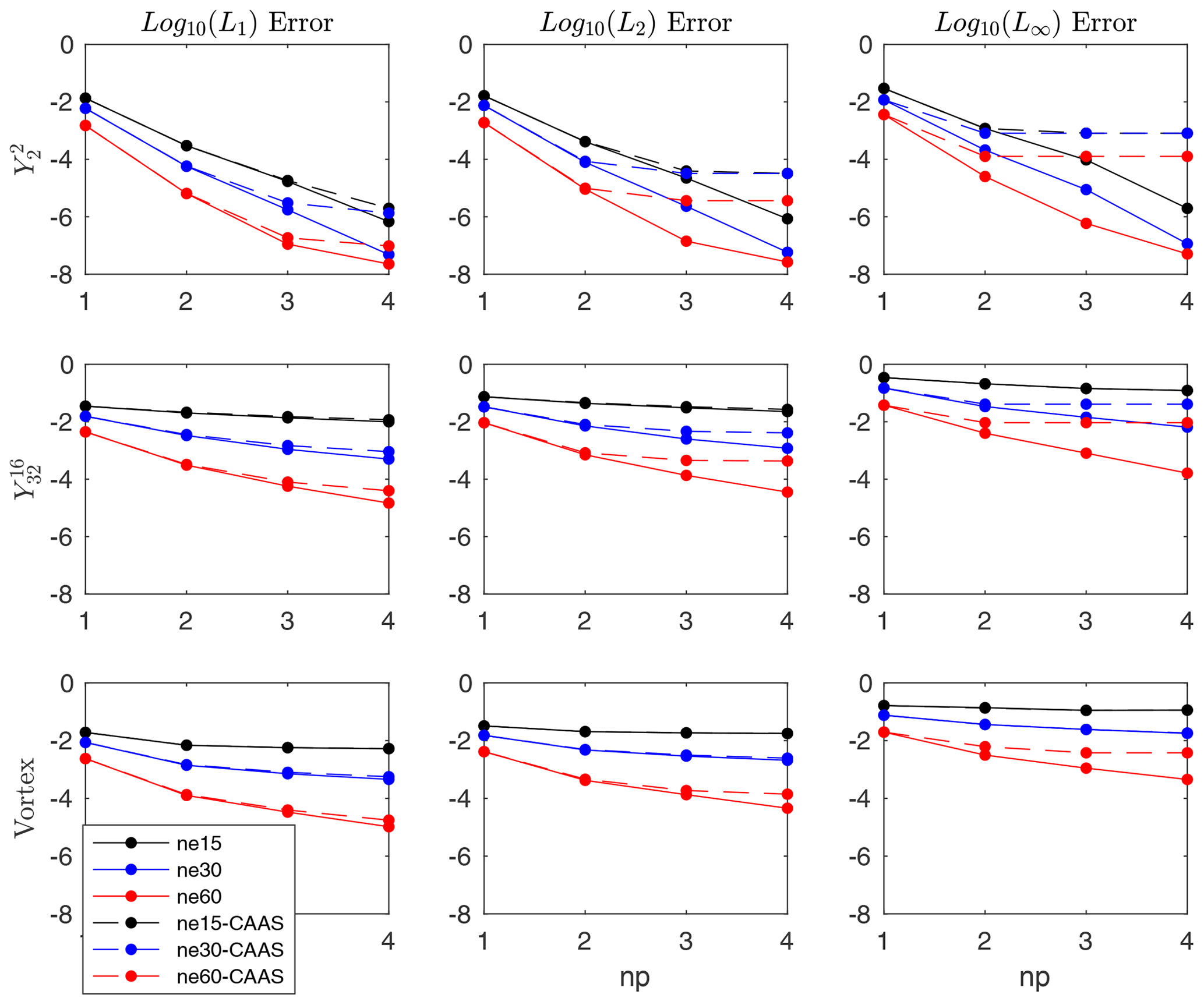
Figure 1 Convergence test for finite-volume to finite-volume remapping from cubed spheres to a 1^∘ latitude–longitude mesh for three different test cases. The dashed lines show the results using CAAS with local-p bounds preservation, and the solid lines are the results without CAAS.

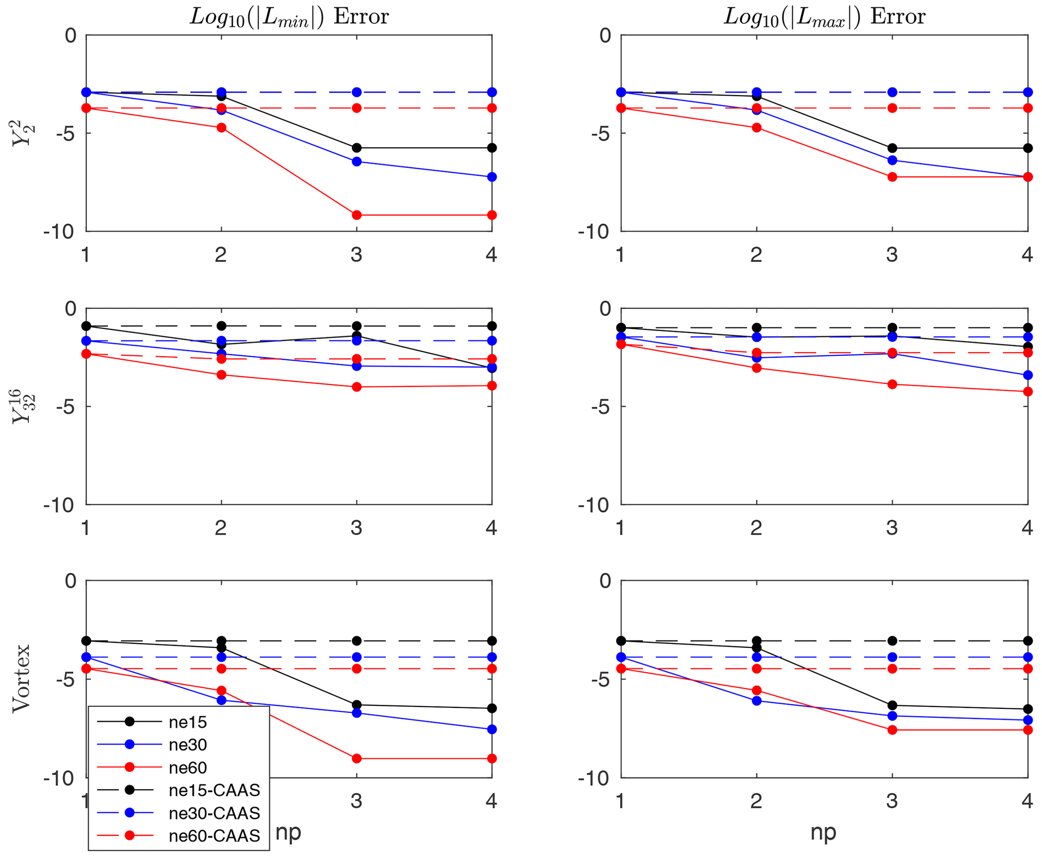
Figure 2 Convergence test for finite-volume to finite-volume remapping from a cubed sphere to a 1^∘ latitude–longitude mesh for three different test cases. Note that in all cases for np>1, the remapped field overshoots and undershoots the absolute maximum and minimum, respectively.

In all cases, the L₁ convergence for the remapped field both with and without CAAS is very similar, and the L₂ convergence is qualitatively similar as well. However, the L_∞ error levels off for all three test cases when CAAS is applied, particularly for the high-resolution cases. This can be understood by looking at the convergence of the corresponding L_min and L_max errors. For all test cases, the remapped field overshoots and undershoots the global maximum and minimum of D^t(ψ): that is, ψ evaluated on the target mesh. The CAAS algorithm will then clip these fields so that, at the very least, they respect the global bounds of ψ evaluated on the source mesh, D^s(ψ). In this case, the remapped field, after applying CAAS to it, will satisfy the inequality $\text{min}{\mathbf{D}}^{\mathrm{s}}\left(\mathit{\psi }\right)\le \mathbf{R}{\mathit{\psi }}^{\mathrm{s}}\le \text{max}{\mathbf{D}}^{\mathrm{s}}\left(\mathit{\psi }\right)$. The effect of the clipping operation, then, is that the L_∞ error will be approximately as large as

$$\begin{array}{}\text{(17)}& min\left(\right|max{\mathbf{D}}^{\mathrm{t}}\left(\mathit{\psi }\right)-max{\mathbf{D}}^{\mathrm{s}}\left(\mathit{\psi }\right)|,|min{\mathbf{D}}^{\mathrm{t}}\left(\mathit{\psi }\right)-min{\mathbf{D}}^{\mathrm{s}}\left(\mathit{\psi }\right)\left|\right)\end{array}$$

because the minimum and maximum of the remapped field after applying CAAS to it will be approximately equal to minD^t(ψ) and maxD^t(ψ). As can be seen in Fig. 2, the L_min and L_max errors remain essentially constant for all mesh resolutions as the order of the polynomial reconstruction is increased. This constancy then results in an effective lower bound on the L_∞ errors and is the reason for the flat lines for the $Y_{\mathrm{2}}^{\mathrm{2}}$, $Y_{\mathrm{32}}^{\mathrm{16}}$, and vortex test cases.

3.2 Finite-element to finite-volume

Here, we examine bounds preservation in the case in which the source mesh is finite-element. Local bounds preservation is defined similarly to how it was for finite-volume source meshes, but now the minimum and maximum in Eq. (14) are computed over all GLL nodes on all the faces that intersect target face i. The convergence results for standard remapping with and without CAAS with local bounds preservation for several different fields are presented in Figs. 3 and 4. Here, the convergence results are nearly identical, apart from the L_∞ error for fourth-order reconstruction for the $Y_{\mathrm{2}}^{\mathrm{2}}$ test case on the coarsest mesh. By looking at the corresponding L_min and L_max errors, we see that the remapped field undershoots and overshoots the global minimum and maximum of D^t(ψ). The error induced by CAAS will once again be approximately equal to the expression given in Eq. (17).

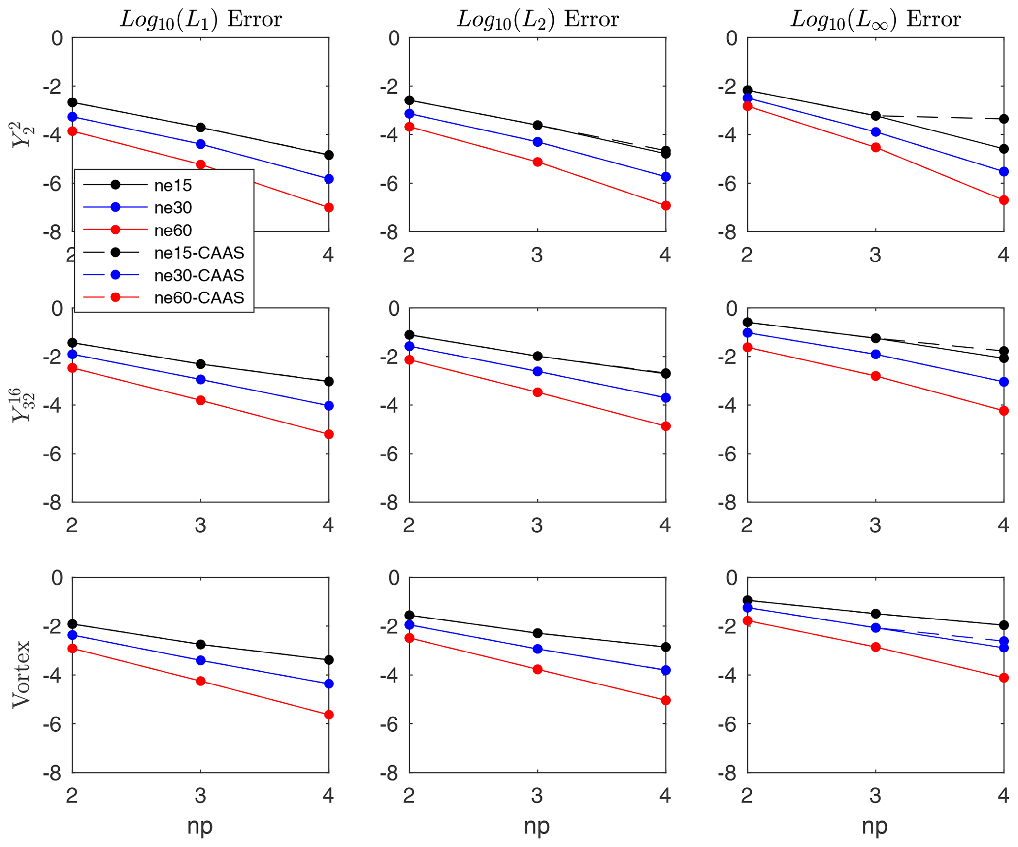
Figure 3 Convergence test for finite-element to finite-volume remapping from a cubed sphere to latitude–longitude mesh using local bounds preservation for three different test cases. The setup is the same as it was for finite-volume to finite-volume remapping, with the dashed lines showing the results using CAAS with local bounds preservation and the solid lines showing the results without CAAS.

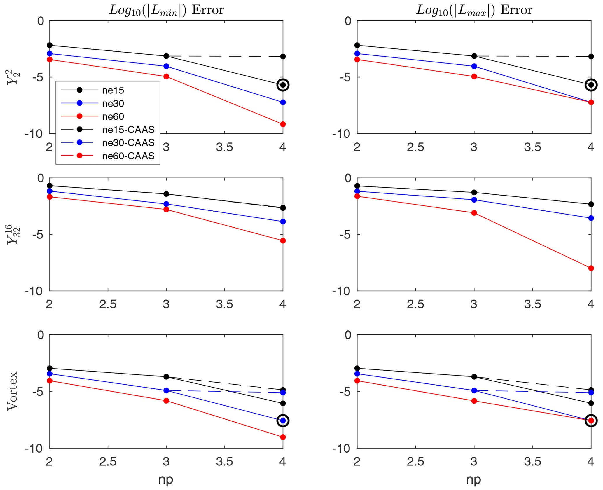
Figure 4 The L_max and L_min results of the convergence test for finite-element to finite-volume remapping from a cubed sphere to a latitude–longitude mesh using local bounds preservation for three different test cases. Circled data points indicate that the global minimum and maximum have been enhanced.

3.3 The Gibbs phenomenon

In this section, we examine the effectiveness of CAAS in reducing overshoots and undershoots associated with remapping a discontinuous source field. To that end, we modify the vortex test case by defined by Eq. (10) by letting the field be equal to zero if it is less than a certain threshold and equal to 1 if it is greater than it.

In Fig. 5, results are shown for four different schemes applied to the vortex test: remapping without CAAS, CAAS with local bounds preservation, CAAS with local-p bounds preservation, and CAAS with global bounds preservation. By global bounds preservation, we mean that the remapped field satisfies the equation

$$\begin{array}{}\text{(18)}& \text{min}{\mathbf{D}}^{\mathrm{s}}\left(\mathit{\psi }\right)\le \mathbf{R}{\mathit{\psi }}^{\mathrm{s}}\le \text{max}{\mathbf{D}}^{\mathrm{s}}\left(\mathit{\psi }\right).\end{array}$$

It is evident from this figure that without applying CAAS, the remapped field suffers from a significant loss of accuracy close to the discontinuity, and significant undershoots of the global minimum are present. The fields obtained using CAAS with local bounds, local-p bounds, and global bounds preservation all show a reduction of oscillations and an improvement of accuracy, with the local bounds preservation resulting in the greatest improvement. One-dimensional cross sections of the remapped fields allow us to examine this reduction more closely. In particular, observe from Fig. 6 how sharply CAAS with local bounds represents the discontinuity. Although the remapped fields obtained using CAAS with local-p bounds and global bounds remain between zero and unity, there are still slight oscillations near zero.

Figure 5 The Gibbs oscillations for a finite-volume to finite-volume remapping from a resolution 60 cubed sphere to a 1^∘ latitude–longitude mesh, with fourth-order polynomial reconstruction. Panel (a) shows the results without CAAS, panel (b) shows the results using CAAS with local bounds preservation, panel (c) shows the results using CAAS with local-p bounds preservation, and panel (d) shows the results using CAAS with global bounds preservation.

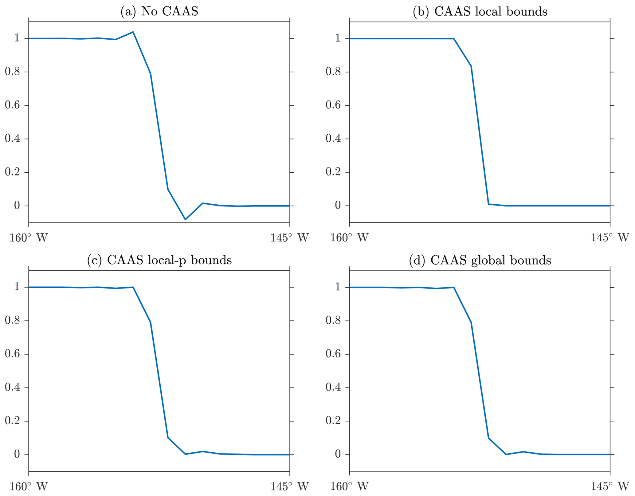
Figure 6 One-dimensional cross sections for remapping of a discontinuous field at the Equator. Panel (a) shows the results without CAAS, (b) shows the results using CAAS with local bounds preservation, (c) shows the results using CAAS with local-p bounds preservation, and (d) shows the results using CAAS with global bounds preservation.

3.4 Real data

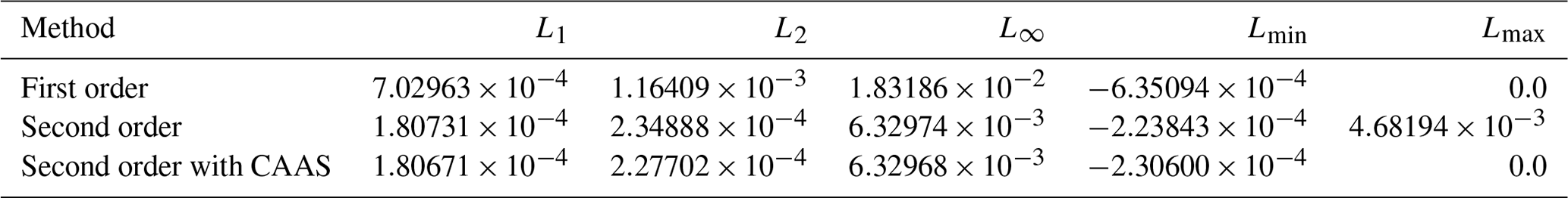
To test the performance of the CAAS algorithm on real data, we use the cloud fraction data generated from the MIRA real data emulator (Mahadevan et al., 2022), which is a field that is required to be bounded between zero and unity and is shown in Fig. 7. We perform two tests. The first is remapping the cloud fraction from an ne90 cubed sphere mesh to a 1^∘ latitude–longitude mesh, and the second is from an ne360 cubed sphere to a 0.25^∘ latitude–longitude mesh. In each case, we compare the accuracy of first order, second order, and second order using CAAS with global bounds preservation between zero and unity. We see from Tables 1 and 2 that the CAAS algorithm gives the smallest error norms for all metrics in both tests.

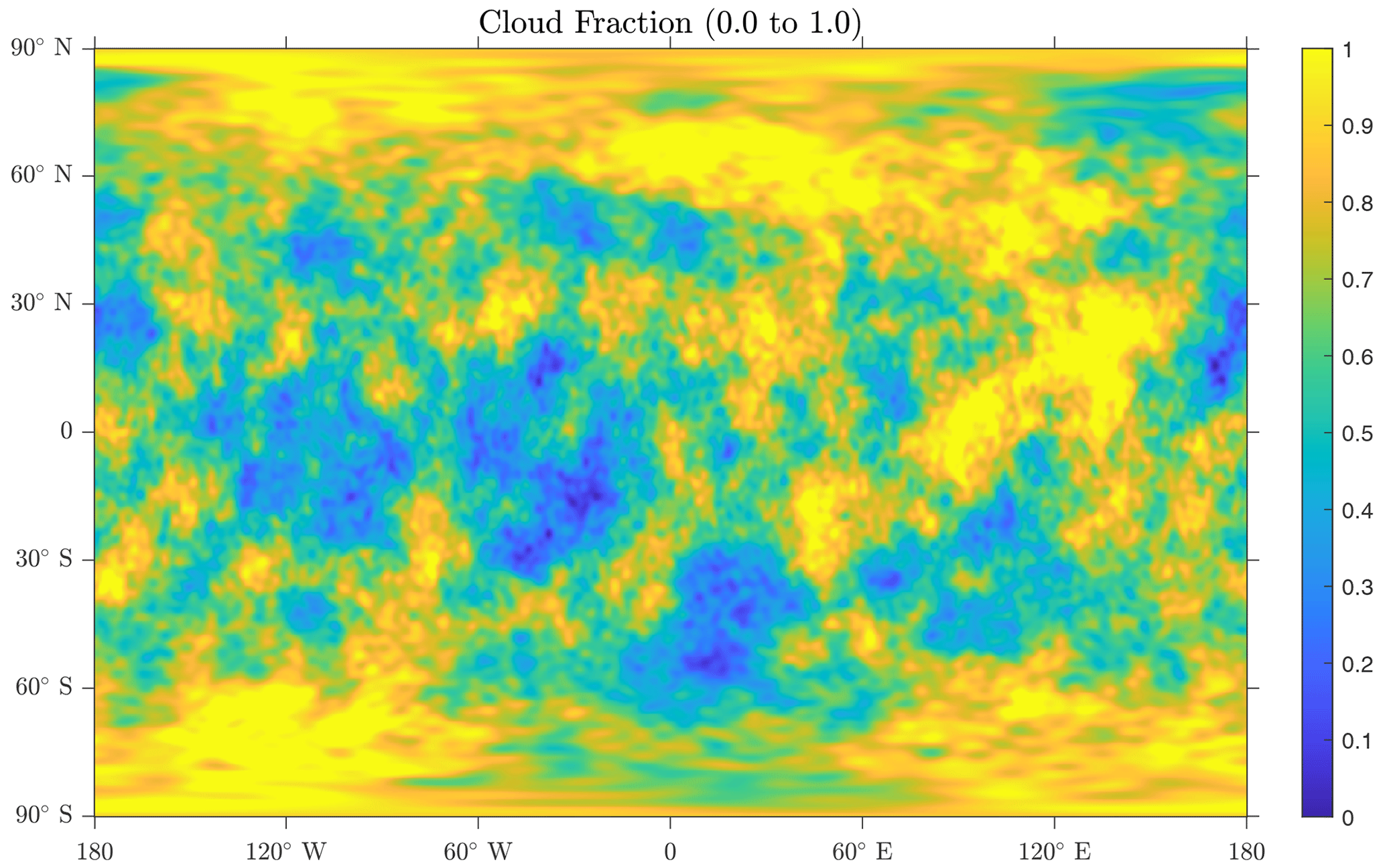
Figure 7 The cloud fraction field used in evaluating the effectiveness of CAAS on a real data field.

Table 1 Error norms for remapping from an ne90 cubed sphere to a 1^∘ latitude–longitude mesh.

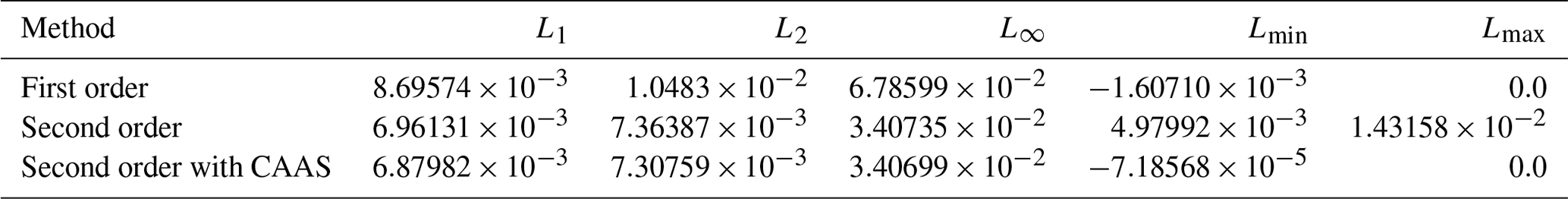
Table 2 Error norms for remapping from an ne360 cubed sphere to a 0.25^∘ latitude–longitude mesh.

4 Non-conservative monotone remapping

In this section, we describe several different approaches to monotone remapping that are consistent but non-conservative. In general, traditional approaches to monotone remapping perform poorly when the source mesh is significantly finer than the target mesh. To correct this, we propose what we call integrated approaches to remapping, which rely on the construction of the overlap mesh or supermesh (e.g., Farrell et al., 2009). This is in contrast to the more traditional approaches that amount to pointwise interpolations, which we refer to as non-integrated approaches, and are used extensively in, for instance, the Earth System Modeling Framework (Hill et al., 2004).

In brief, for consistent and monotone remapping operators, we express the value of ψ^t at each spatial degree of freedom on the target mesh as a weighted sum of N values of ψ^s:

$$\begin{array}{}\text{(19)}& {\mathit{\psi }}_j^{\mathrm{t}}=w_{i_{\mathrm{1}}}{\mathit{\psi }}_{i_{\mathrm{1}}}^{\mathrm{s}}+\mathrm{\dots }+w_{i_N}{\mathit{\psi }}_{i_N}^{\mathrm{s}},\end{array}$$

where i_k denotes the index of a spatial degree of freedom on the source mesh. As we are working with finite-volume meshes in this context, the spatial degrees of freedom correspond to the average value over the mesh faces. For consistency, we need $w_{i_{\mathrm{1}}}+\mathrm{\dots }+w_{i_N}=\mathrm{1}$, and for monotonicity, we need $\mathrm{0}\le w_{i_{\mathrm{1}}},\mathrm{\dots },w_{i_N}\le \mathrm{1}$. The weights $w_{i_k}$ then make up the entries of the remapping operator R given in Eq. (1).

4.1 Bilinear remapping

Here, we describe the non-integrated approach to monotone bilinear remapping found in the ESMF. Suppose we are given a point on the target mesh onto which we are remapping. Call this point P_j. First, we need to find a triangle or quadrilateral whose vertices are source face centers that contains P_j. We assume that the edges of these triangles and quadrilaterals are great-circle arcs. Now the source mesh is described in terms of the nodes of each face and the edges that connect them. Since the field values at the face centroids represent second-order approximations to the average value of the field, they are the natural choice for interpolation. To that end, the dual mesh of the source mesh is constructed, which will result in a mesh whose faces have source face centroids as their vertices. Once the dual mesh is available, it can be searched to find a polygon that contains P_j, the given point on the target mesh. If the polygon that contains P_j has more than four sides, it is triangulated in order to find a sub-triangle that contains P_j.

Once this polygon is found, and assuming it has to be further triangulated, we solve the following equation:

$$\begin{array}{}\text{(20)}& (\mathrm{1}-\mathit{\alpha }-\mathit{\beta }){\mathit{Q}}_{i_{\mathrm{1}}}+\mathit{\alpha }{\mathit{Q}}_{i_{\mathrm{2}}}+\mathit{\beta }{\mathit{Q}}_{i_{\mathrm{3}}}=(\mathrm{1}-\mathit{\gamma }){\mathit{P}}_j,\end{array}$$

where ${\mathit{Q}}_{i_{\mathrm{1}}}$, ${\mathit{Q}}_{i_{\mathrm{2}}}$, and ${\mathit{Q}}_{i_{\mathrm{3}}}$ are the coordinates of the face centers of the triangle that contains P_j. Intuitively, the solution to this equation corresponds to first finding the intersection of the line through the origin and P_j, and the plane that passes through the points ${\mathit{Q}}_{i_{\mathrm{1}}}$, ${\mathit{Q}}_{i_{\mathrm{2}}}$, and ${\mathit{Q}}_{i_{\mathrm{3}}}$, and then representing this point as a linear combination of these three points. The coefficients in Eq. (20) then define the value of the remapped field on the target mesh:

$$\begin{array}{}\text{(21)}& {\mathit{\psi }}_j^{\mathrm{t}}=(\mathrm{1}-\mathit{\alpha }-\mathit{\beta }){\mathit{\psi }}_{i_{\mathrm{1}}}^{\mathrm{s}}+\mathit{\alpha }{\mathit{\psi }}_{i_{\mathrm{2}}}^{\mathrm{s}}+\mathit{\beta }{\mathit{\psi }}_{i_{\mathrm{3}}}^{\mathrm{s}}.\end{array}$$

Note that we have assumed that P_j is the center of the jth face on the target mesh. The weights clearly sum to 1, and they are non-negative because triangle ${\mathit{Q}}_{i_{\mathrm{1}}}{\mathit{Q}}_{i_{\mathrm{2}}}{\mathit{Q}}_{i_{\mathrm{3}}}$ contains P_j. Hence, this weighting defines a monotone, consistent remapping operator (Ullrich and Taylor, 2015). The case in which the polygon that contains P_j has four sides is similar. In particular, we solve the equation

$$\begin{array}{}\text{(22)}& \begin{array}{rl}(\mathrm{1}-\mathit{\alpha })& (\mathrm{1}-\mathit{\beta }){\mathit{Q}}_{i_{\mathrm{1}}}+\mathit{\alpha }(\mathrm{1}-\mathit{\beta }){\mathit{Q}}_{i_{\mathrm{2}}}+\mathit{\alpha }\mathit{\beta }{\mathit{Q}}_{i_{\mathrm{3}}}\\ & +\mathit{\beta }(\mathrm{1}-\mathit{\alpha }){\mathit{Q}}_{i_{\mathrm{4}}}=(\mathrm{1}-\mathit{\gamma }){\mathit{P}}_j,\end{array}\end{array}$$

where ${\mathit{Q}}_{i_{\mathrm{1}}}$ to ${\mathit{Q}}_{i_{\mathrm{4}}}$ are vertices of the quadrilateral that contains P_j. The coefficients in the previous equation then results in the equation

$$\begin{array}{}\text{(23)}& \begin{array}{rl}{\mathit{\psi }}_j^{\mathrm{t}}& =(\mathrm{1}-\mathit{\alpha })(\mathrm{1}-\mathit{\beta }){\mathit{\psi }}_{i_{\mathrm{1}}}^{\mathrm{s}}+\mathit{\alpha }(\mathrm{1}-\mathit{\beta }){\mathit{\psi }}_{i_{\mathrm{2}}}^{\mathrm{s}}\\ & +\mathit{\alpha }\mathit{\beta }{\mathit{\psi }}_{i_{\mathrm{3}}}^{\mathrm{s}}+\mathit{\beta }(\mathrm{1}-\mathit{\alpha }){\mathit{\psi }}_{i_{\mathrm{4}}}^{\mathrm{s}}.\end{array}\end{array}$$

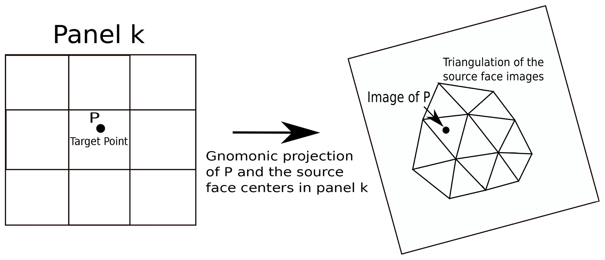
Figure 8 An overview of the Delaunay triangulation remapping scheme, whereby the images of the source face centers are triangulated.

Figure 9 The weights used in the weighting based on the Delaunay triangulation.

4.1.1 Delaunay triangulation remapping

In this section, we describe an alternative to the remapping scheme described in the previous section. We obviate the need to triangulate an arbitrary polygon by constructing the Delaunay triangulation of the face centroids of the source mesh. We outline our approach as follows. We seek a triangle on the source mesh whose vertices are source face centroids that contains a given point on the target mesh. To that end, we divide the sphere into six panels: call them R_i for $\mathrm{1}\le i\le \mathrm{6}$. The panels $R_{\mathrm{1}},\mathrm{\dots },R_{\mathrm{4}}$ are equally sized and lie along the Equator between 45^∘ N and 45^∘ S. The panels R₅ and R₆ are equally sized caps above and below 45^∘ N and 45^∘ S, respectively. Let S_i denote gnomonic projections of the set of source face centroids in R_i onto the plane tangent to the sphere at the center of R_i. So S_i is a set of two-dimensional points, and we denote its Delaunay triangulation by T(S_i) (Shewchuk, 1996). So given a point P_j on the target mesh, we first find the panel R_k that contains it. We then compute G(P_j), the gnomonic projection onto the plane tangent to the sphere at the center of R_k. We then find the triangle with vertices ${\mathit{V}}_{i_{\mathrm{1}}},{\mathit{V}}_{i_{\mathrm{2}}}$, and ${\mathit{V}}_{i_{\mathrm{3}}}\in T\left(S_k\right)$ that contains G(P_j). To find this triangle, we use a k–d tree. First, we use the tree to find the triangle whose center is nearest G(P_j). If G(P_j) is in this triangle, we stop. Otherwise we search through neighboring triangles until we find one that contains it. A summary of this process is shown in Fig. 8, where a triangulation of the images of the source face centers under the gnomonic projection is shown. Now we know that the gnomonic projection maps great-circle arcs on the sphere to straight lines on the plane, so if ${\mathit{P}}_{i_{\mathrm{1}}}$, ${\mathit{P}}_{i_{\mathrm{2}}}$, and ${\mathit{P}}_{i_{\mathrm{3}}}$ are the points on the source mesh such that $G\left({\mathit{P}}_{i_{\mathrm{1}}}\right)={\mathit{V}}_{i_{\mathrm{1}}}$, $G\left({\mathit{P}}_{i_{\mathrm{2}}}\right)={\mathit{V}}_{i_{\mathrm{2}}}$, and $G\left({\mathit{P}}_{i_{\mathrm{3}}}\right)={\mathit{V}}_{i_{\mathrm{3}}}$, then we can be sure that P_j is contained within the spherical triangle whose vertices are ${\mathit{P}}_{i_{\mathrm{1}}}$, ${\mathit{P}}_{i_{\mathrm{2}}}$, and ${\mathit{P}}_{i_{\mathrm{3}}}$. We then approximate the value of ${\mathit{\psi }}_j^{\mathrm{t}}$ as

$$\begin{array}{}\text{(24)}& {\mathit{\psi }}_j^{\mathrm{t}}={\displaystyle \frac{A_{i_{\mathrm{1}}}}{A}}{\mathit{\psi }}_{i_{\mathrm{1}}}^{\mathrm{s}}+{\displaystyle \frac{A_{i_{\mathrm{2}}}}{A}}{\mathit{\psi }}_{i_{\mathrm{2}}}^{\mathrm{s}}+{\displaystyle \frac{A_{i_{\mathrm{3}}}}{A}}{\mathit{\psi }}_{i_{\mathrm{3}}}^{\mathrm{s}},\end{array}$$

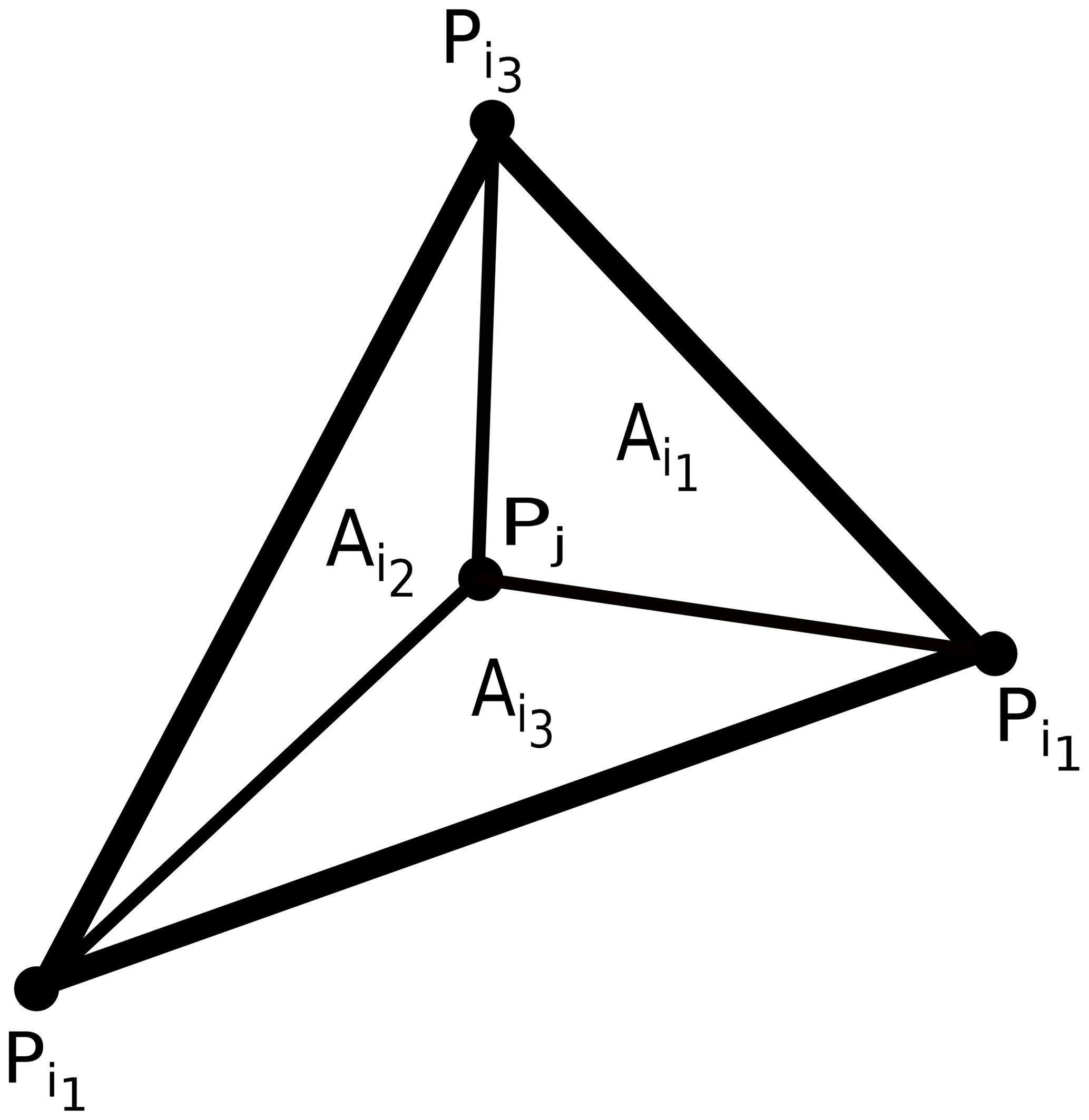
where, as can be seen in Fig. 9, $A_{i_k}$ is the area of the spherical sub-triangle that does not have ${\mathit{P}}_{i_k}$ as a vertex, and A is the area of the spherical triangle that contains P_j. The weights are non-negative because they correspond to triangle areas, and they are between zero and 1 because $\mathrm{0}\le A_{i_k}\le A$. Hence, these weights are monotone and consistent. Note that an advantage of this approach is that it is easily parallelized, as we can divide the sphere into an arbitrary number of panels.

4.1.2 Generalized barycentric coordinate remapping

The final scheme we describe is based on what are called generalized barycentric coordinates (Floater, 2015). Our use of this scheme is motivated by a desire for a systematic way of incorporating more source points into Eq. (19). Intuitively, we expect such a scheme to give more accurate results, as it would incorporate more information from nearby source points for each point on the target mesh. We first define these coordinates and then provide a description of where we expect them to be most useful. Let ${\mathit{P}}_{\mathrm{1}},\mathrm{\dots },{\mathit{P}}_n$ be the vertices of a polygon in the plane and Q be a point within the polygon. The generalized barycentric coordinates of Q with respect to the vertices, w_i, satisfy the following.

1. ${\displaystyle }{\sum }_{i=\mathrm{1}}^n{w}_i=\mathrm{1}$

2. w_i≥0

3. ${\displaystyle }{\sum }_{i=\mathrm{1}}^n{w}_i\left(\mathit{x}\right){\mathit{P}}_i=\mathit{x}$

The first two properties are responsible for consistency and monotonicity, and the third property, known as linear precision, means that linear functions can be reconstructed exactly in terms of the polygon vertices and is essentially why these weights are second-order accurate. One particular set of weights is given by the equation

$$\begin{array}{}\text{(25)}& w_i=A({\mathit{P}}_{i-\mathrm{1}},{\mathit{P}}_i,{\mathit{P}}_{i+\mathrm{1}})\prod _{k\ne i,i-\mathrm{1}}A(\mathit{Q},{\mathit{P}}_k,{\mathit{P}}_{k+\mathrm{1}}),\end{array}$$

where $A({\mathit{P}}_{i-\mathrm{1}},{\mathit{P}}_i,{\mathit{P}}_{i+\mathrm{1}})$ and $A(\mathit{Q},{\mathit{P}}_k,{\mathit{P}}_{k+\mathrm{1}})$ denote the areas of triangles ${\mathit{P}}_{i-\mathrm{1}}{\mathit{P}}_i{\mathit{P}}_{i+\mathrm{1}}$ and QP_kP_k+1, respectively, and w_i is the weight corresponding to vertex P_i (Meyer et al., 2002).

We generalize to the sphere by interpreting the areas in Eq. (25) as the areas of spherical triangles, rather than planar triangular areas. An advantage of these weights is that they are general; they can be used for arbitrary polygons, not just triangles and quadrilaterals.

As was the case with bilinear interpolation outlined in Sect. 4.1, the dual of the source mesh is constructed. This will provide a mesh whose nodes are source face centers that can be searched through efficiently. We again use a k–d tree to find the dual mesh face that contains a target point Q. The details are similar to those described for the Delaunay triangulation scheme in Sect. 4.1.1. Once we have this face, we apply the weights given in Eq. (25). We point out that for the triangular meshes we are considering, most faces on the dual mesh are hexagonal, so using the generalized barycentric coordinates given in Eq. (25) will allow up to six source points to be incorporated into the remapping operator in Eq. (19), instead of the three or four points that would be used for the Delaunay triangulation weighting given in Eq. (24), or the bilinear weighting in Eq. (21). We hypothesize that this doubling of the number of source points in Eq. (19) would lead to an increase in accuracy for remapping fields on triangular source meshes. Furthermore, the generalized barycentric coordinate weighting will always incorporate at least as many source points as either other scheme.

4.2 Non-integrated remapping: numerical tests

Here we show the results of two different numerical tests. In the first case, the remapping is done from cubed spheres to a fixed 1^∘ latitude–longitude mesh. The cubed spheres are of increasing resolution with n_e=5, 10, 20, 40, 80, and 160 and have 150, 600, 2400, 9600, 38 400, and 153 600 faces, respectively. The target mesh has 64 800 faces. We plot the error norms as functions of the approximate face size, which we take to be the square root of the approximate area of each face. Specifically, the face size is defined as

$$\begin{array}{}\text{(26)}& \text{face size}=\sqrt{{\displaystyle \frac{\mathrm{4}\mathit{\pi }}{N}}},\end{array}$$

where N is the number of faces. We see from Fig. 10 that the schemes converge at second order and are approximately similar in magnitude.

Figure 10 Convergence results for several non-integrated monotone remapping schemes for a fixed latitude–longitude target mesh and cubed sphere source meshes.

For the second test, the target is still a fixed 1^∘ latitude–longitude mesh, and the source meshes are triangular geodesic meshes with 180, 720, 2880, 11 520, 46 080, and 184 320 faces. From Fig. 11, we see that all schemes converge at second order and give similar error norms in most cases. For the high-frequency and vortex tests, however, we see that the generalized barycentric scheme gives consistently smaller L_∞ errors than the Delaunay triangulation and the bilinear schemes, which indicates that the generalized barycentric weighting is slightly more effective at resolving the sharp gradients present in these fields. So although we hypothesized that the generalized barycentric coordinates would perhaps give a more noticeable improvement in the errors for all cases for triangular source meshes, we found that its benefit appears to be limited to the L_∞ errors for the $Y_{\mathrm{32}}^{\mathrm{16}}$ and vortex fields.

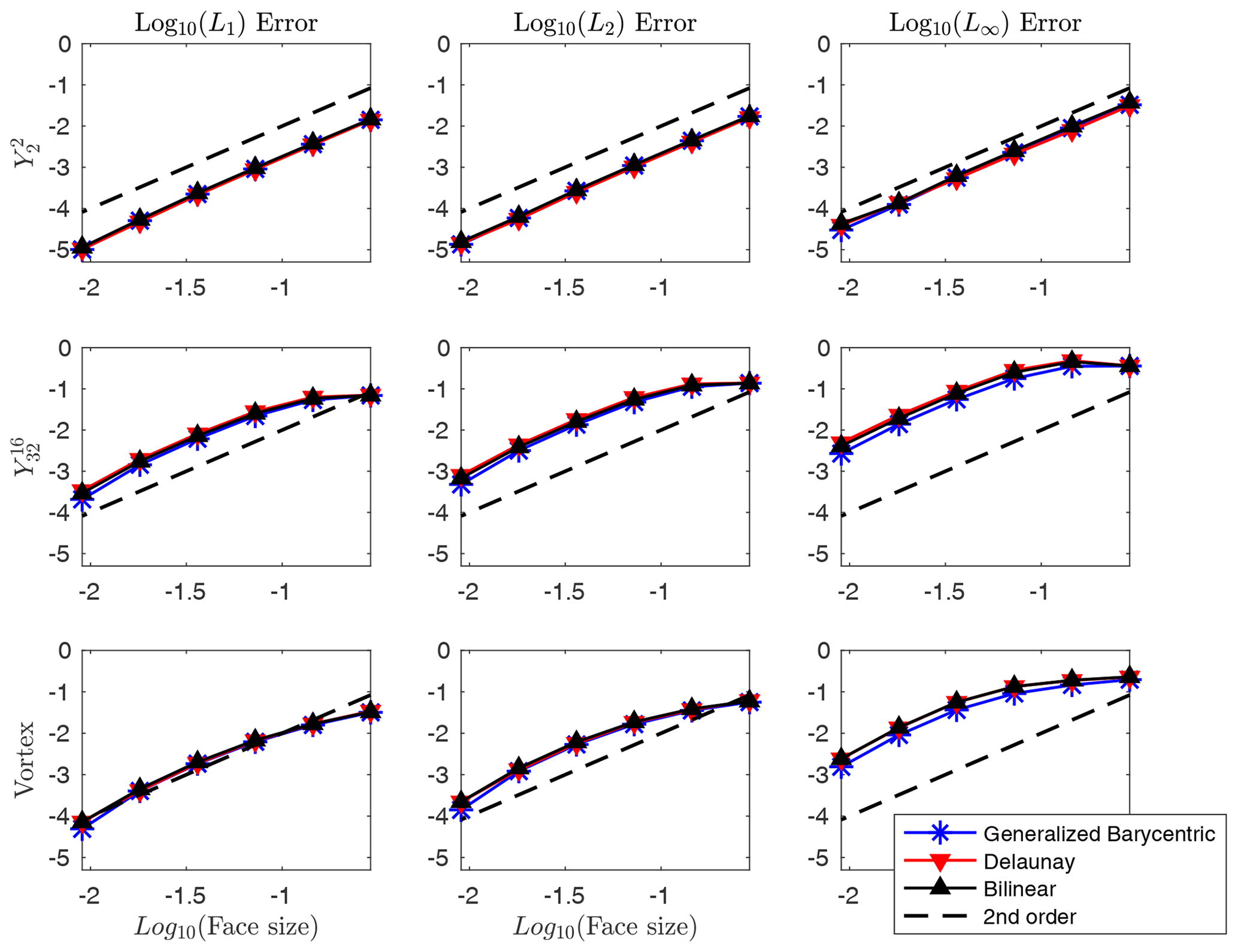
Figure 11 Convergence results for several non-integrated monotone remapping schemes for a fixed latitude–longitude target mesh and triangular source meshes.

Figure 12 Convergence results for several integrated monotone remapping schemes for a fixed latitude–longitude target mesh and cubed sphere source meshes.

4.3 Integrated remapping

The remapping schemes described in the previous sections work well when the source mesh is not too much finer than the target mesh. However, when the resolution of the source mesh is greater than that of the target mesh, pointwise sampling of the source mesh to determine a field value on the target mesh is inappropriate and inaccurate. In this case, a large number of points on the source mesh contribute no weights to the remapping operator. To combat this under-sampling, we now describe an approach that ensures all points on the source mesh are sampled via construction of the overlap mesh or supermesh. Approaches of this type are called integrated because of their analog to numerical quadrature and are distinguished from the non-integrated approaches described in Sect. 4.1–4.1.2. A non-integrated approach basically amounts to an interpolation, whereby we express each value of the target field as a weighted sum of nearby source values. In the integrated approach, we recall that our variables correspond to face averages, and we approximate these integrals via quadrature. Specifically, for each face on the target mesh, we apply triangular quadrature to each sub-triangle of each overlap face, where the number of overlap faces is determined by the source mesh faces that intersect the given target face. Written out in full, we have

$$\begin{array}{}\text{(27)}& {\mathit{\psi }}_i^{\mathrm{t}}\approx {\displaystyle \frac{\mathrm{1}}{\left|{\mathrm{\Omega }}_i^{\mathrm{t}}\right|}}{\displaystyle }\sum _{j=\mathrm{1}}^{N_{\mathrm{ov}}}{\displaystyle }\sum _{k=\mathrm{1}}^{N_{\mathrm{t}}}{\displaystyle }\sum _{m=\mathrm{1}}^{N_{\mathrm{q}}}{\mathit{\psi }}^{\mathrm{s}}\left({\mathit{x}}_{m,k,j}\right)\mathrm{d}{W}_m,\end{array}$$

where $\left|{\mathrm{\Omega }}_i^{\mathrm{t}}\right|$ is the area of target face i, N_ov is the number of source faces that overlap target face i, N_T is the number of sub-triangles per overlap face, N_q is the number of quadrature points per sub-triangle, dW_m is the quadrature weight for the mth quadrature point, and ${\mathit{x}}_{m,k,j}$ is the location of the mth quadrature point within each sub-triangle of each overlap face. Now we do not know the value of ${\mathit{\psi }}^{\mathrm{s}}\left({\mathit{x}}_{m,k,j}\right)$, so we need to estimate it. In our numerical tests, we will use all three of the weightings described in Sect. 4. In particular, we estimate ${\mathit{\psi }}^{\mathrm{s}}\left({\mathit{x}}_{m,k,j}\right)$ as

$$\begin{array}{}\text{(28)}& {\mathit{\psi }}^{\mathrm{s}}\left({\mathit{x}}_{m,k,j}\right)={\displaystyle }\sum _{l=\mathrm{1}}^N{w}_l{\mathit{\psi }}_{p_{i_l}}^{\mathrm{t}},\end{array}$$

where the $p_{i_{\mathrm{1}}}$ to $p_{i_N}$ denote the faces on the source mesh whose centers form the polygon that contains ${\mathit{x}}_{m,k,j}$, and $w_{\mathrm{1}},\mathrm{\dots },w_{i_N}$ represent the corresponding weights given by Eqs. (24), (25), and (21) or (23), depending on the source mesh. Because the integration is performed by way of the overlap mesh, we can be sure that every degree of freedom on the source mesh contributes weights to the remapping operator.

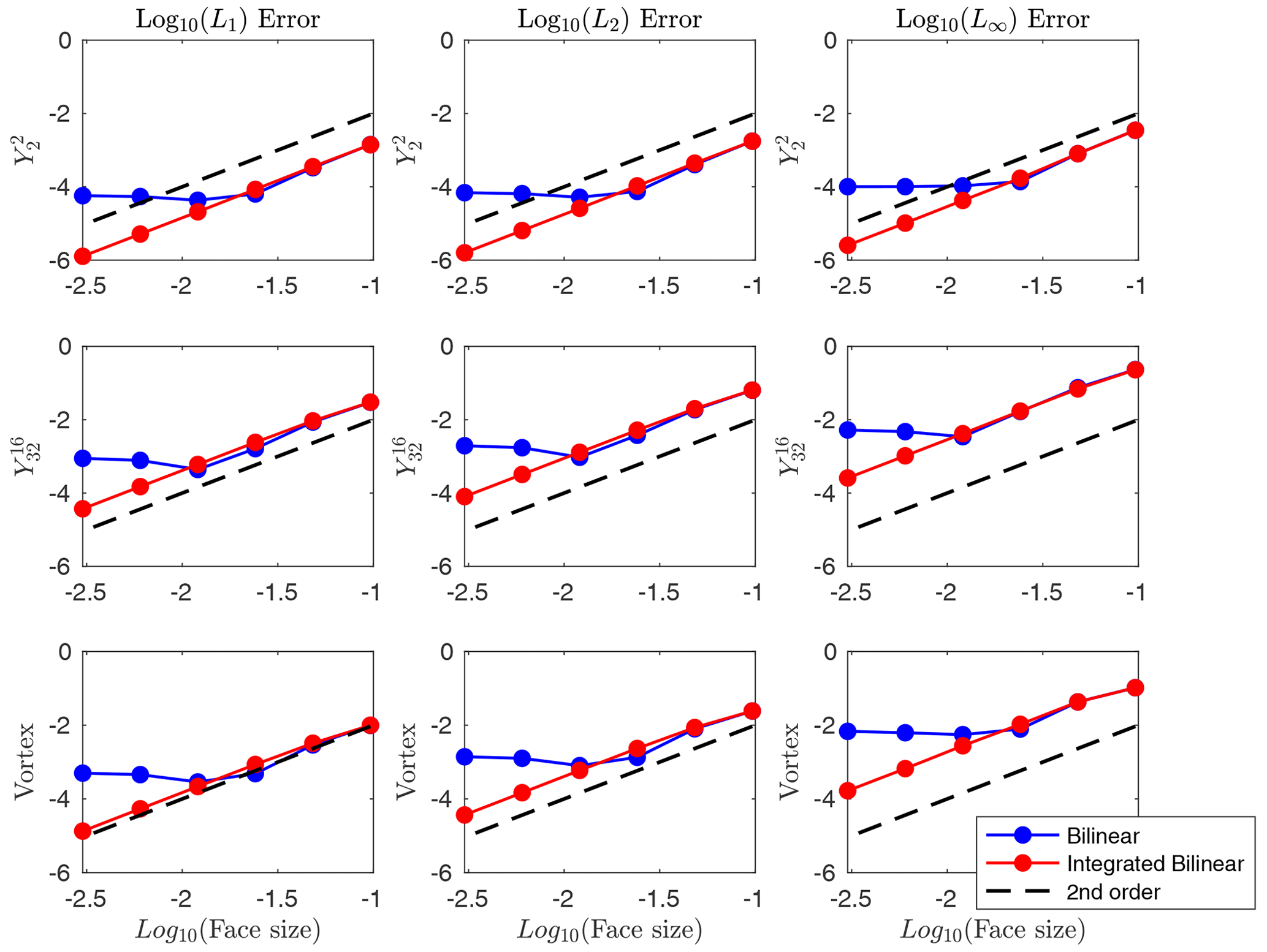
Figure 13 Convergence results for the integrated and non-integrated bilinear remapping schemes from cubed spheres to a fixed latitude–longitude mesh.

4.4 Integrated remapping: numerical tests

This section again consists of two tests. The first test is to establish second-order convergence of the integrated schemes, and it is identical to the setup of the first test shown in Sect. 4.2. In Fig. 12, we compare the results of the integrated versions of all three remapping schemes described in Sect. 4. All three schemes give error norms similar to their non-integrated counterparts shown in Fig. 10. In particular, the error norms of the generalized barycentric and bilinear schemes are nearly identical. This is to be expected, as in both schemes, the value at each point on the target mesh depends on four source points.

In the next test, we consider a setup wherein the source meshes are refined beyond the resolution of the target mesh. The source meshes are cubed spheres with n_e=15, 30, 60, 120, 240, and 480 and have 1350, 5400, 21 600, 86 400, 345 600, and 1 382 400 faces, respectively. The target mesh is a fixed latitude–longitude mesh of 2^∘ resolution. We see from Fig. 13 that the accuracy of the non-integrated scheme is degraded, but the integrated scheme remains second-order. In particular, observe that the accuracy of the non-integrated bilinear scheme starts to diminish relative to the integrated one when the face size is between 10^−1.5 and 10⁻², which corresponds to a source mesh with no more than approximately 125 000 faces. Before this point, the errors of both schemes are similar. We point out that we only include a comparison of the integrated and non-integrated versions of the bilinear scheme, as the results look nearly identical for both the generalized barycentric and Delaunay triangulation schemes.

5 Conclusion

In this paper we have examined a number of different schemes for conservative and non-conservative monotone remapping. For monotone conservative remapping, we showed that the “clip and assured sum” method provides an accurate way of remapping conservative fields that are required to stay bounded and is effective at reducing the Gibbs-like oscillations associated with discontinuous source fields.

We then described several different approaches to non-conservative remapping. Two of these have, to the best of our knowledge, never been applied to remapping problems on the sphere. These methods have what are referred to as non-integrated and integrated versions, and it was shown that the integrated versions are capable of maintaining second-order accuracy across a wide range of source mesh resolutions by systematically sampling the degrees of freedom on the source mesh, albeit at higher computational costs.

As discussed in the Introduction, the methods described in this paper have been implemented as part of v2.1.6 of the TempestRemap software package (Ullrich et al., 2022).