Porting the WAVEWATCH III (v6.07) wave action source terms to GPU

Surface gravity waves play a critical role in several processes, including mixing, coastal inundation, and surface fluxes. Despite the growing literature on the importance of ocean surface waves, wind–wave processes have traditionally been excluded from Earth system models (ESMs) due to the high computational costs of running spectral wave models. The development of the Next Generation Ocean Model for the DOE’s (Department of Energy) E3SM (Energy Exascale Earth System Model) Project partly focuses on the inclusion of a wave model, WAVEWATCH III (WW3), into E3SM. WW3, which was originally developed for operational wave forecasting, needs to be computationally less expensive before it can be integrated into ESMs. To accomplish this, we take advantage of heterogeneous architectures at DOE leadership computing facilities and the increasing computing power of general-purpose graphics processing units (GPUs). This paper identifies the wave action source terms, W3SRCEMD, as the most computationally intensive module in WW3 and then accelerates them via GPU. Our experiments on two computing platforms, Kodiak (P100 GPU and Intel(R) Xeon(R) central processing unit, CPU, E5-2695 v4) and Summit (V100 GPU and IBM POWER9 CPU) show respective average speedups of 2× and 4× when mapping one Message Passing Interface (MPI) per GPU. An average speedup of 1.4× was achieved using all 42 CPU cores and 6 GPUs on a Summit node (with 7 MPI ranks per GPU). However, the GPU speedup over the 42 CPU cores remains relatively unchanged (∼ 1.3×) even when using 4 MPI ranks per GPU (24 ranks in total) and 3 MPI ranks per GPU (18 ranks in total). This corresponds to a 35 %–40 % decrease in both simulation time and usage of resources. Due to too many local scalars and arrays in the W3SRCEMD subroutine and the huge WW3 memory requirement, GPU performance is currently limited by the data transfer bandwidth between the CPU and the GPU. Ideally, OpenACC routine directives could be used to further improve performance. However, W3SRCEMD would require significant code refactoring to make this possible. We also discuss how the trade-off between the occupancy, register, and latency affects the GPU performance of WW3.

1 Introduction

Ocean surface gravity waves, which derive energy and momentum from steady winds blowing over the surface of the ocean, are a very crucial aspect of the physical processes at the atmosphere–ocean interface. They influence a variety of physical processes such as momentum and energy fluxes, gas fluxes, upper-ocean mixing, sea spray production, ice fracture in the marginal ice zone, and Earth albedo (Cavaleri et al., 2012). Such complex wave processes can only be treated accurately by including a wave model into Earth system models (ESMs). The first ocean models neglected the existence of ocean waves by assuming that the ocean surface is rigid to momentum and buoyancy fluxes from the atmospheric boundary layer (Bryan and Cox, 1967). Currently, most state-of-the-science ESMs are still missing some or all of these wave-induced effects (Qiao et al., 2013), despite the growing literature on their importance in the simulation of weather and climate.

Recent literature has shown that incorporating different aspects of surface waves into ESMs leads to improved skill performance, particularly in the simulation of sea surface temperature, wind speed at 10 m height, ocean heat content, mixed-layer depth, and the Walker and Hadley circulations (Law Chune and Aouf, 2018; Song et al., 2012; Shimura et al., 2017; Qiao et al., 2013; Fan and Griffies, 2014; Li et al., 2016). Yet, only two climate models that participated in the Climate Model Intercomparison Project Phase 6 (CMIP6), i.e., the First Institute of Oceanography Earth System Model Version 2 (FIO-ESM v2.0; Bao et al., 2020) and the Community Earth System Model Version 2 (CESM2; Danabasoglu et al., 2020), have a wave model as part of their default model components. However, for CMIP6, only FIO-ESM v2.0 employed a wave model. Wind–wave-induced physical processes have traditionally been excluded from ESMs due to the high computational cost of running spectral wave models on global model grids for long-term climate integrations. In addition to higher computing costs due to longer simulation times, adding new model components also increases resource requirements (e.g., the number of central processing units/nodes). The next-generation ocean model development in the US Department of Energy (DOE) Energy Exascale Earth System Model (E3SM) project partly focuses on the inclusion of a spectral wave model, WAVEWATCH III (WW3), into E3SM to improve the simulation of coastal processes within E3SM. To make WW3 within E3SM feasible for long-term global integrations, we need to make it computationally less expensive.

Computer architectures are evolving rapidly, especially in the high-performance computing environment, from traditional homogeneous machines with multicore central processing units (CPUs) to heterogeneous machines with multi-node accelerators such as graphics processing units (GPUs) and multicore CPUs. Moreover, the number of CPU–GPU heterogeneous machines in the top 10 of the TOP500 increased from two in November 2015 (https://www.top500.org/lists/top500/2015/11/, last access: 30 November 2022) to seven in November 2022 (https://www.top500.org/lists/top500/2022/11/, last access: 30 November 2022). The advent of heterogeneous super-computing platforms as well as the increasing computing power and low energy-to-performance ratio of GPUs has motivated the use of GPUs to accelerate climate and weather models. In recent years, numerous studies have reported successful GPU porting of full or partial weather and climate models with improved performance (Hanappe et al., 2011; Xu et al., 2015; Yuan et al., 2020; Zhang et al., 2020; Bieringer et al., 2021; Mielikainen et al., 2011; Michalakes and Vachharajani, 2008; Shimokawabe et al., 2010; Govett et al., 2017; Li and Van Roekel, 2021; Xiao et al., 2013; Norman et al., 2017; Norman et al., 2022; Bertagna et al., 2020). A GPU programming model is different from CPU code, so programmers must recode or use directives to port codes to GPU. Because climate and weather models consist of million of lines of code, a majority of the GPU-based climate simulations only operate on certain hot spots (most computationally intensive operations) of the model while leaving a large portion of the model on CPUs. In recent years, however, efforts have been made to run an entire model component on a GPU. For example, Xu et al. (2015) ported the entire Princeton Ocean Model to GPU and achieved a 6.9× speedup. Similarly, the entire E3SM atmosphere including SCREAM (Simple Cloud-Resolving E3SM Atmosphere Model) is running on a GPU (https://github.com/E3SM-Project/scream, last access: 30 November 2022). Taking advantage of the recent advancements in GPU programming in climate sciences and the heterogeneous architectures at DOE leadership computing facilities, this study seeks to identify and move the computationally intensive parts of WW3 to GPU through the use of OpenACC pragmas.

The rest of the paper is structured as follows: Sect. 2 presents an overview of the WW3 model and its parallelization techniques, give an introduction to the OpenACC programming model, describe the hardware and software environment of our testing platforms, and finally present the test case configuration used in this study; the results section, Sect. 3, presents the WW3 profiling analysis on CPU, discusses the challenges encountered, outlines GPU-specific optimization techniques, and compares the GPU results with the original Fortran code; and Sect. 4 concludes the paper.

2 Model description and porting methodology

2.1 WAVEWATCH III

WW3 is a third-generation spectral wave model developed at the US National Centers for Environmental Prediction (NOAA/NCEP) (WAVEWATCH III® Development Group, 2019) from the WAve Model (WAM) (The Wamdi Group, 1988). It has been widely used to simulate ocean waves in many oceanic regions for various science and engineering applications (Chawla et al., 2013b; Alves et al., 2014; Cornett, 2008; Wang and Oey, 2008). To propagate waves, WW3 solves the random-phase spectral action density balance equation, $N(\mathit{\varphi },\mathit{\lambda },\mathit{\sigma },\mathit{\theta },t)$, for wave number direction spectra. The intrinsic frequency (σ) relates the action density spectrum to the energy spectrum (F), $N=\frac{F}{\mathit{\sigma }}$. For large-scale applications, the evolution of the wave action density in WW3 is expressed in spherical coordinates as follows:

$$\begin{array}{}\text{(1)}& {\displaystyle \frac{\partial N}{\partial t}}+{\displaystyle \frac{\partial \left(C_{\mathit{\varphi }}N\right)}{\partial \mathit{\varphi }}}+{\displaystyle \frac{\partial \left(C_{\mathit{\lambda }}N\right)}{\partial \mathit{\lambda }}}+{\displaystyle \frac{\partial \left(C_{\mathit{\sigma }}N\right)}{\partial \mathit{\sigma }}}+{\displaystyle \frac{\partial \left(C_{\mathit{\theta }}N\right)}{\partial \mathit{\theta }}}=\sum _i{S}_i.\end{array}$$

Equation (1) is solved by discretizing in both physical space (λ, ϕ) and spectral space (σ, θ). Here, ϕ is the longitude, λ is the latitude, σ is the relative frequency, θ is the direction, t is time, and S represents the source and sinks terms. The net source–sink terms consist of several physical processes responsible for the generation, dissipation, and redistribution of energy. The net source–sink terms available in WW3 are wave generation due to wind (S_in), dissipation (S_ds), nonlinear quadruplet interactions (S_nl), bottom friction (S_bt), and depth-limited breaking (S_db); triad wave–wave interactions (S_tr); scattering of waves by bottom features (S_sc); wave–ice interactions (S_ice); and reflection off shorelines or floating objects (S_ref). Details of each source term can be found in the WW3 manual (WAVEWATCH III® Development Group, 2019). The primary source–sink terms used in this work are S_in, S_ds, S_nl, S_bt, and S_db. Several modules are used for the calculation of source terms. However, the W3SRCEMD module manages the general calculation and integration of source terms.

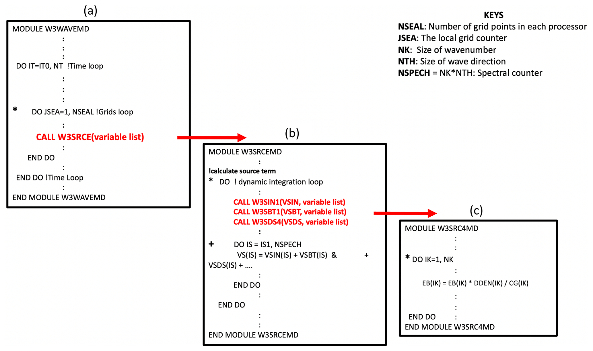
When moving code between different architectures, it is necessary to understand its structure. For the purposes of our study, Fig. 1 shows a representation of the WW3 algorithm structure. WW3 is divided into several submodules, but the actual wave model is W3WAVEMD, which runs the wave model for a given time interval. Within W3WAVEMD, several modules are called at each time interval to handle initializations, interpolation of winds and currents, spatial propagation, intra-spectral propagation, calculation and integration of source terms, output file processing, etc. In our work, we found that W3SRCEMD is the most computationally intensive part of WW3; thus, we focus our attention on this module. According to Fig. 1a, W3SRCEMD is being called at each spatial grid point, which implies that the spatial grid loop is not contained in W3SRCEMD but rather in W3WAVEMD. Figure 1b, which represents W3SRCEMD, contains a dynamic integration time loop that can only be executed sequentially. It also calls a number of submodules, such as W3SRC4MD for the computation of the wind input and wave breaking dissipation source terms. W3SRCEMD consists of collapsed spectral loops $(\mathrm{NSPECH}=\mathrm{NK}\times \mathrm{NTH})$, where NK is the number of frequencies (σ) and NTH is the number of wave directions (θ). Lastly, W3SRC4MD (Fig. 1c) consists of only frequency (NK) loops. The structure of other source terms submodules is similar to W3SRC4MD.

Figure 1 A schematic representation of the WAVEWATCH III code structure.

2.2 WW3 grids and parallel concepts

The current version of WW3 can be run and compiled for both single- and multiprocessor Message Passing Interface (MPI) compute environments with regular grids, two-way nested (mosaic) grids (Tolman, 2008), spherical multicell (SMC) grids (Li, 2012), and unstructured triangular meshes (Roland, 2008; Brus et al., 2021). In this study, we ran and compiled WW3 using an MPI with unstructured triangular meshes as the grid configuration. In WW3, the unstructured grid can be parallelized in physical space using either card deck (CD) (Tolman, 2002) or domain (Abdolali et al., 2020) decomposition. Following Brus et al. (2021), we used the CD approach as the parallelization strategy. The ocean (active) grid cells are sorted and distributed linearly between processors in a round-robin fashion using $n=\mathrm{mod}(m-\mathrm{1},N)$, i.e., grid cell m is assigned to processor n. Here, N is the total number of processors. If N is divisible by M (the total number of ocean grids), every processor n has the same number of grids, NSEAL (Fig. 1a). The source term calculation as well as the intra-spectral propagation are computed using the aforementioned parallel strategy, but data are gathered on a single processor to perform the spatial propagation.

2.3 OpenACC

To demonstrate the promise of GPU computing for WW3, we used the OpenACC programming model. OpenACC is a directive-based parallel programming model developed to run codes on accelerators without significant programming effort. Programmers incorporate compiler directives in the form of comments into Fortran, C, or C++ source codes to assign the computationally intensive sections of the code to be executed on the accelerator. OpenACC helps to simplify GPU programming because the programmer is not preoccupied with the code parallelism details, unlike CUDA and OpenCL where you need to change the code structure to achieve GPU compatibility. The OpenACC compiler automatically transfers calculations and data between two different architectures: the host (CPU) and the accelerator device (GPU). OpenACC works together with OpenMP, MPI, and CUDA, supporting heterogeneous parallel environments. Starting from version 4.5, the OpenMP API (application programming interface) specification has been extended to include GPU offloading and GPU parallel directives. Whereas OpenMP and OpenACC have similar constructs, OpenMP is more prescriptive. Prescriptive directives describe the exact computation that should be performed and provide the compiler no flexibility. Our study focuses solely on OpenACC because it has the most mature implementation using the NVIDIA compiler on NVIDIA GPUs at the time of analysis.

Table 1 GPU hardware specifications.

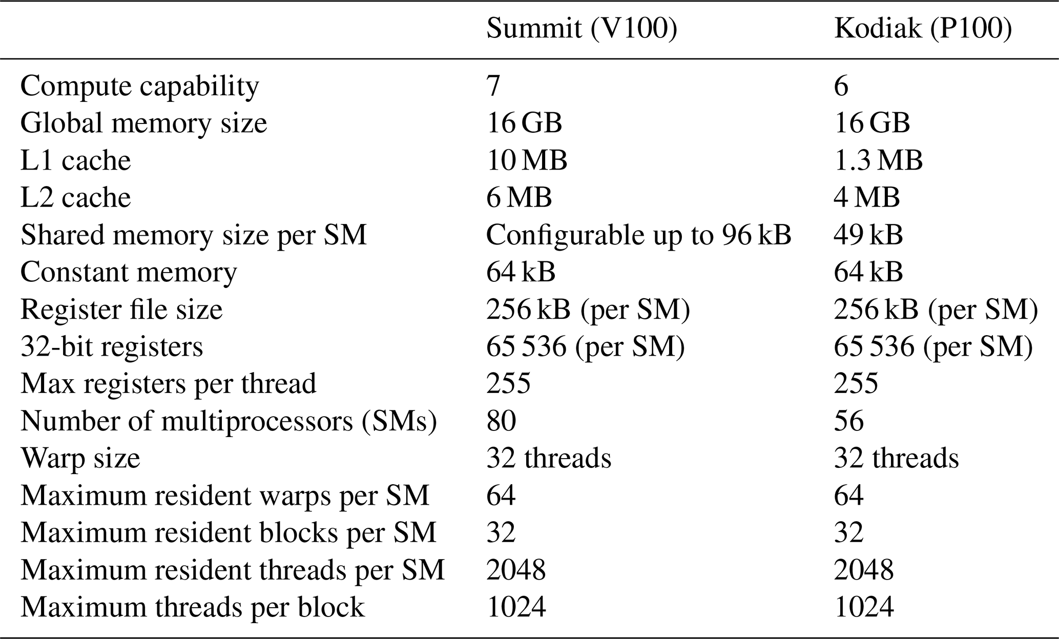
SM refers to streaming multiprocessor, and L1 and L2 denote Level 1 and Level 2, respectively.

OpenACC has three levels of parallelism (Fig. 2), namely vectors, workers, and gangs, corresponding to threadIdx.x, threadIdx.y, and blockIdx.x in CUDA terminology. A gang is a group of workers, where multiple gangs work independently without synchronization. Workers are groups of vectors/threads within a gang, and a vector is the finest level of parallelism operating with single-instruction, multiple thread (SIMT). Gangs, workers, and vectors can be added to a loop region that needs to be executed on a GPU. An example of Fortran code with and without OpenACC directives is shown in Fig. 3. The OpenACC directives are shown in green as comments starting with !$acc (e.g., lines 6 and 12 in Fig. 3b). In Fig. 3b, line 6 is a declaration directive for allocating memory for variables on GPU, line 8 is the data region to move data into the GPU, line 11 updates data already present on the GPU with new values from the CPU, line 12 launches the parallel region at the gang level and then dispatches the parallel threads at the worker and vector levels, line 21 updates CPU data with new values from the GPU, and line 28 deletes the data on the GPU after computation. To learn more about all OpenACC directives, the reader is referred to NVIDIA (2017) or Chandrasekaran and Juckeland (2017)

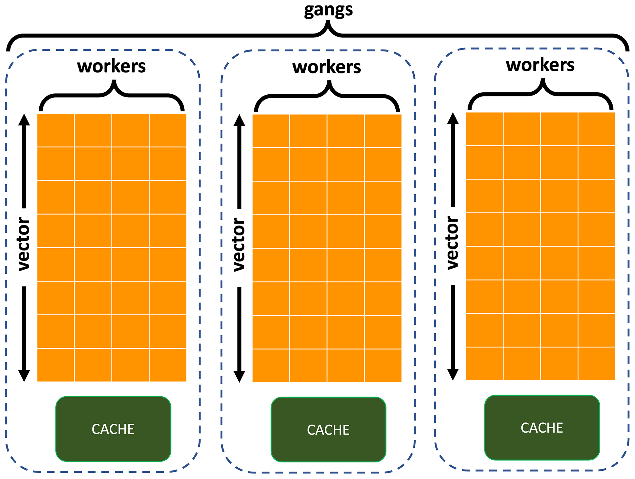
Figure 2 A map of gangs, workers, and vectors (adapted from Jiang et al., 2019).

2.4 Test case configuration

In this study, the WW3 model was configured and simulated over the global ocean with an unstructured mesh with a 1^∘ global resolution and a 0.25^∘ resolution in regions with a depth of less than 4 km, e.g., 1^∘ at the Equator and 0.25^∘ in coastal regions (Brus et al., 2021). The number of the unstructured mesh nodes is 59 072 (ranges from 1^∘ at the Equator to 0.5^∘ along coastlines; hereafter 59K). In addition, we demonstrate the effect of scaling the problem size on speedup by using an unstructured mesh with 228 540 nodes (ranges from 0.5^∘ at the Equator to 0.25^∘ along coastlines; hereafter 228K). Following Chawla et al. (2013a), for both spatial grid configurations, we use a spectral grid that has 36 directions and 50 frequency bands that range exponentially from 0.04 to 0.5 Hz, separated by a factor of 1.1. In WW3, the combinations and types of the source terms in Eq. (1) depend on the research question being answered. WW3 has several source term packages which can be implemented by activating different switches. However, as the goal of this study is purely computational, we selected the following commonly used source–sink term switches: ST4, DB1, BT1, and NL1. The ST4 switch (Ardhuin et al., 2010) consists of the wind input (S_in) and wave breaking dissipation (S_ds) source terms, the DB1 switch is for the depth-induced breaking (S_db) source term, the BT1 switch consists of the bottom friction (S_bt) source term parameterizations, and the nonlinear quadruplet wave interactions (S_nl) are computed in the model using the NL1 switch.

We develop and test our accelerated WW3 code on GPUs on the following two computational platforms with heterogeneous architectures:

1. the Kodiak cluster from the Parallel Reconfigurable Observational Environment (PROBE) facility (Gibson et al., 2013) of Los Alamos National Laboratory. Kodiak has 133 compute nodes. Each node contains an Intel(R) Xeon(R) CPU (E5-2695 v4), 2.10 GHz with 36 CPU cores, and four NVIDIA Tesla P100 SXM2 general purpose computation on graphics processing units (GPGPUs), each with 16 GB of memory.

2. Summit, a high-performance computing system at Oak Ridge National Laboratory (ORNL). Summit has 4608 nodes; each node contains two IBM POWER9 CPUs and six NVIDIA Tesla V100 GPUs, each with 80 streaming multiprocessors. All are connected together with NVIDIA’s high-speed NVLink. Summit is the fastest supercomputer in the US and the second fastest in the world (in 2021).

Table 1 shows the configuration of each compute node for both platforms. For a more accurate comparison of CPU and GPU codes, we used the same compiler. On Kodiak, the CPU Fortran code was compiled using the flags -g -O3 -acc. Similarly, the OpenACC code was compiled with flags -g -O3 -acc -Minfo=accel -ta=tesla,ptxinfo,maxregcount:n. Likewise, the flags for the CPU code on Summit are -g -O2, and those of OpenACC are -g -O2 -acc -ta=tesla,ptxinfo,maxregcount:n -Minfo=accel. Options -ta=tesla:ptxinfo,maxregcount:n are the optimization flags¹ used in this study (Sect. 3.2). Adding the option -ta=tesla:ptxinfo to the compile flags provides information about the amount of shared memory used per kernel (a function that is called by the CPU for execution on the GPU) as well the registers per thread. The flag -ta=tesla:maxregcount:n, where “n” is the number of registers, sets the maximum number of registers to use per thread.

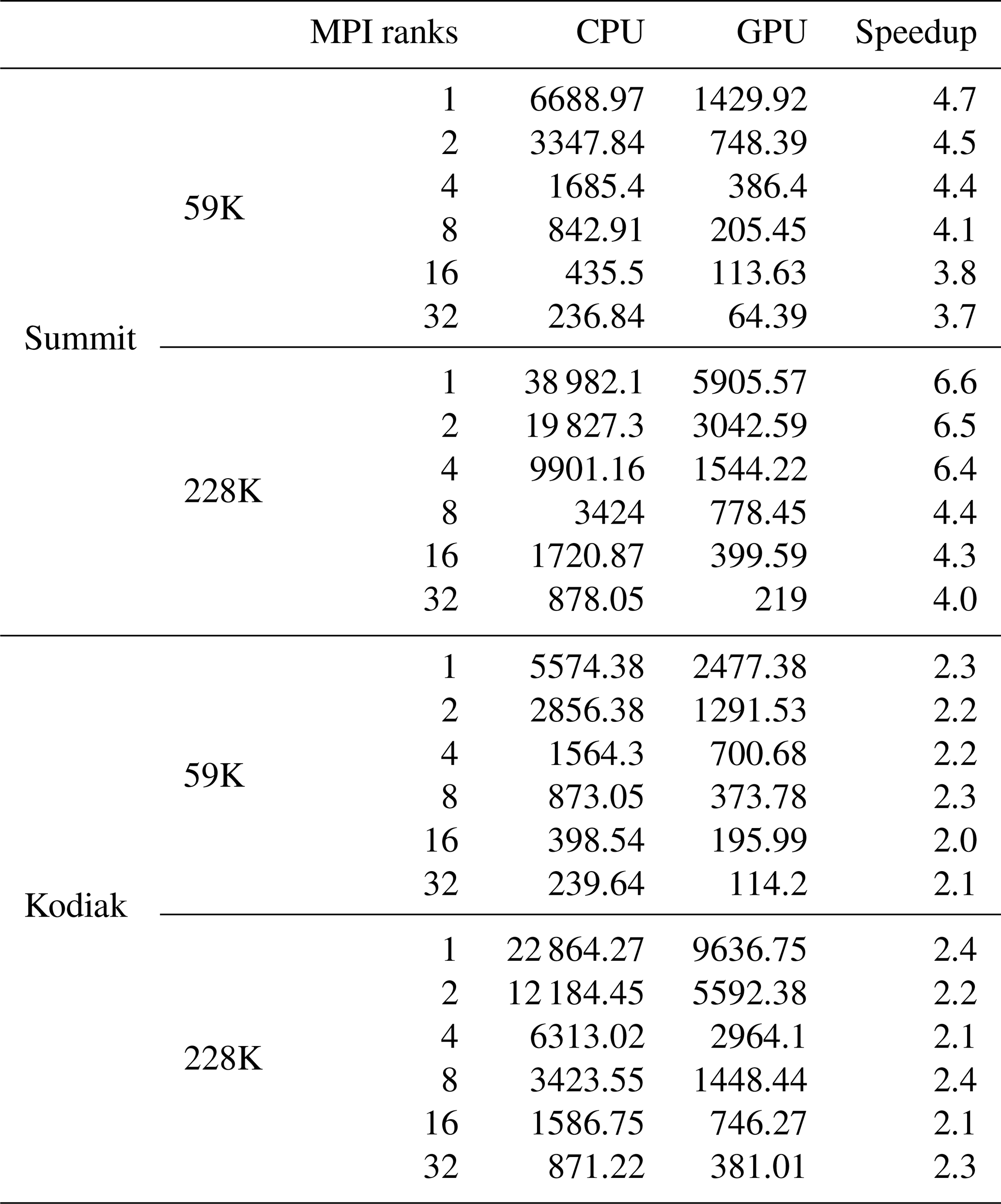
Table 2 The speedups and simulation times associated with offloading one MPI rank exclusively to one GPU on Kodiak and Summit with 59K and 228K mesh sizes for MPI ranks ranging from 1 to 32.

As a test case, we performed a 5 h simulation from 00:00:00 to 05:00:00 on 1 June 2005 by forcing WW3 with atmospheric winds derived from the US National Center for Atmospheric Research (NCAR) reanalysis. We verify the GPU model for correctness using significant wave heights (SWHs) from the CPU-only simulation.

3 Results and evaluations

In this section, we first describe the performance of WW3 on a CPU and its computationally intensive sections. Furthermore, we discuss the challenges encountered, how GPU optimization is done, and present the performance result of porting WW3 on GPU. Lastly, we discuss the performance limitation using roofline analysis.

3.1 WW3 profiling analysis on a CPU

With model optimization, an important step is to find the runtime bottlenecks by measuring the performance of various sections in units of time and operations. In order to not waste time nor resources improving the performance of rarely used subroutines, we first need to figure out where WW3 spends most of its time. The technical term for this process is “profiling”. For this purpose, we profile WW3 by running the Callgrind profiler from the Valgrind tool and then visualize the output using a KCachegrind tool (Weidendorfer, 2008). An application's performance can be 10× to 50× slower when profiling it with Callgrind; however, the proportions of time remain the same. Figure 4 shows the call graph obtained by profiling WW3 with 300 MPI ranks. The source term subroutine, W3SRCEMD, can easily be spotted as the consumer of ∼ 82 % of the total execution time and resources. Within the W3SRCEMD subroutine, the dissipation source term S_ds uses more than 40 % of the total runtime because it contains numerous time-consuming spectral loops. In fact, profiling WW3 with another profiler (not shown), Intel Advisor (Intel Corporation, 2021), specifically highlights the time-consuming spectral loops. In WW3, each processor serially runs through its sets of allocated spatial grids (described in Sect. 2.2), with each containing spectral grid points, and W3SRCEMD has a time-dynamic integration (Fig. 1b) procedure which can not be parallelized. Looping through spectral grids and the time-dynamic integration procedure are plausible reasons why W3SRCEMD is the bottleneck of WW3. We refer to the WW3 model with GPU-accelerated W3SRCEMD as “WW3-W3SRCEMD.gpu”, and we refer to the CPU-only version as “WW3.cpu”.

Fortunately, W3SRCEMD does not contain neighboring grid dependencies in the spatial nor spectral grids, i.e., no parallel data transfers; therefore, W3SRCEMD can be ported to GPUs with less difficulty. We moved the entire WW3 source term computation to GPU, as shown in Fig. 3b.

Figure 3 A schematic representation of the WAVEWATCH III original Fortran source code for the W3WAVEMD module (a) and its OpenACC directives version (b).

3.2 Challenges and optimization

Once the program hot spot is ported to the GPU, the GPU code needs to be optimized in order to improve its performance. Conventionally, the optimization of GPU codes involves loop optimization (fusion and collapse), data transfer management (CPU to GPU and GPU to CPU), memory management, and occupancy. Some of these optimization techniques are interrelated (e.g., memory management and occupancy). The WW3 model contains very few collapsible loops, so loop fusing and loop collapsing did not effectively optimize the code (not shown). To successfully port WW3-W3SRCEMD.gpu and achieve the best performance, two challenges had to be overcome in this study. The first is a data transfer issue caused by the WW3 data structure, while the second is a memory management and occupancy issue caused by the use of many local arrays, sometimes of spectral length, and scalars within W3SRCEMD and its embedded subroutines.

3.2.1 Data transfer management

It is important to understand the layout of data structures in the program before porting to a GPU. WW3 outlines its data structures using modules, e.g., W3ADATMD, W3GDATMD, and W3ODATMD (lines 2 and 3 of Fig. 3a). Depending on the variable required, each subroutine uses these modules. These variables are called global external variables. As it is not possible to move data within a compute kernel in a GPU, all necessary data must be present on the GPU prior to launching the kernel that calls W3SRCEMD. The structure of WW3 requires the use of a routine directive (!$acc routine) to create a device version of W3SRCEMD, as well as other subroutines in it. In Fortran, the routine directive appears in the subprogram specification section or its interface block. Due to the use of routine directives, OpenACC declare directives (!$acc declare create; line 6 of Fig. 3b) were added to the data structures module to inform the compiler that global variables need to be created in the device memory as well as the host memory.

All data must be allocated on the host before being created on a device unless they have been declared device residents. In WW3, however, arrays whose size are determined by spatial–spectral grid information are allocated at runtime, rather than within the data structure modules. Thus, creating data on the device within the WW3 data modules poses a problem. Due to this restriction, it was then necessary to explicitly move all of the required data to the GPU before launching the kernel. For managing data transfers between iteration cycles, we use !$acc update device(variables) and !$acc update self(variables) (lines 11 and 21 in Fig. 3b). However, it would be easier to use unified memory, which offers a unified memory address space to both CPUs and GPUs, rather than tracking each and every piece of data that needs to be sent to the GPU, but the latest OpenACC version does not support the use of unified memory with routine directives. In the future, having this feature would save time spent tracking data transfers in programs with many variables such as WW3.

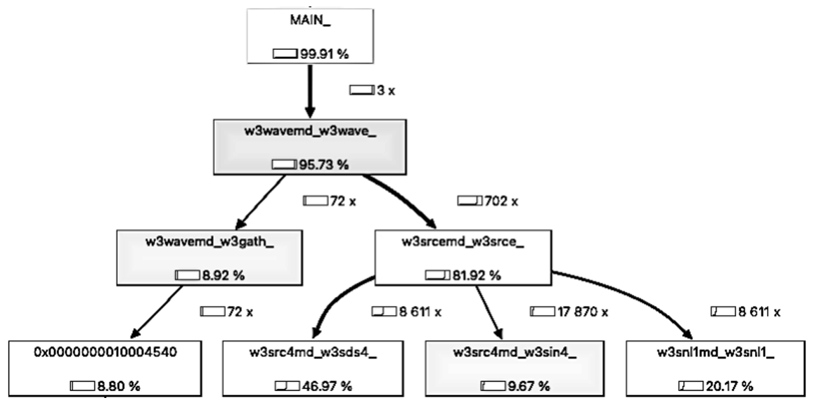
Figure 4 The call graph obtained by profiling WAVEWATCH III with 300 CPU cores on Summit. Each box includes the name of the subroutine and its relative execution time as a percentage.

3.2.2 Memory management and occupancy

Occupancy is defined as the ratio of active warps (workers) on a streaming multiprocessor (SM) to the maximum number of active warps supported by the SM. On Kodiak and Summit, the maximum number of threads per SM is 2048. A warp consists of 32 threads which implies that the total number of possible warps per SM is 8. Even if the kernel launch configuration maximizes the number of threads per SM, other GPU resources, such as shared memory and registers, may also limit the number of maximum threads, thus indirectly affecting GPU occupancy. A register is a small amount of fast storage available to each thread, whereas shared memory is the memory shared by all threads in each SM. As seen in Table 1, the maximum memory per SM for Kodiak and Summit is 256 kB, but the maximum shared memory is 64 kB for Kodiak (P100) and 94 kB for Summit (V100). In terms of total register file size per GPU, Kodiak and Summit have 14 336 and 20 480 kB, respectively.

To estimate GPU usage, we use the CUDA occupancy calculator available at https://docs.nvidia.com/cuda/cuda-occupancy-calculator/CUDA_Occupancy_Calculator.xls (last access: 30 November 2022). In this study, the kernel launch configurations consist of NSEAL gangs, where NSEAL refers to the number of grids on each node, and each gang has 32 vector lengths (or threads). With this configuration, the achievable GPU occupancy (regardless of other resources) is 50 %. Adding -ta=tesla:pxtinfo to the compiler flags provides information about the size of registers, memory spills (movement of variables out of the register space to the main memory), and shared memory allocated during compilation. Kodiak and Summit both allocate the maximum 255 kB register per thread, reducing the GPU occupancy to 13 %. In addition, a full register leads to the spilling of memory into the Level 1 (L1) cache (shared memory). A spill to cache is fine, but a spill to the global memory will severely affect performance because the time required to get data from the global memory is longer than the time required to get data from a register. This phenomenon is known as latency: the amount of time required to move data from one point to the other. Therefore, an increase (decrease) in register size causes two different things simultaneously: a decrease (increase) in occupancy and a decrease (increase) in latency. There is always a trade-off between register, latency, and occupancy, and the trick is to find the spot that maximizes performance. One can set the maximum number of registers per thread via the -ta=tesla:maxregcount:n flag, where “n” is the number of registers.

Figure 5 illustrates how the trade-off between latency and occupancy affects the GPU performance based on the number of registers. Our analysis was only based on the performance of running a 228K mesh configuration with 16 MPI tasks. For Summit, as the number of registers increases from 16 to 64, the GPU occupancy remains constant at 50 % and GPU performance improves due to the movement of more variables to the fast memory. As indicated by the blue part of the line, this is a latency-dominant region. However, as the number of register increases from 64 to 192, GPU occupancy gradually decreases from 50 % to 13 %. This degraded performance despite moving more data into the fast memory. Therefore, this is an occupancy-dominant region, as indicated by the red part of the line (Fig. 5b). From 192 to the maximum register count, the occupancy remains constant at 13 % and GPU performance remains relatively constant. As occupancy is constant, latency is expected to dominate this region, which is represented by the green part of the line in Fig. 5b. However, we observe no memory spill for registers between 192 and 255 and, thus, the latency effect remains unchanged. Therefore, constant latency and occupancy result in constant performance in this region.

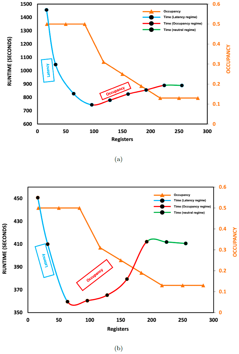
Figure 5 The WW3-W3SRCEMD.gpu runtime (primary vertical axis) and occupancy (secondary vertical axis in orange) based on register counts on Kodiak (a) and Summit (b). For the runtime, the light blue part of the line represents the latency-dominant region, the red part represents the occupancy-dominant region, and the green part represents the neutral region. We analyzed the result of running a 228K mesh size on 16 GPUs and CPUs.

Figure 5b shows that 64 registers produced the best performance (minimum runtime) on Summit. For brevity, the previously described trade-off analysis also applies to Kodiak, and a 96 register count produced the best performance (Fig. 5a). On Kodiak, the register count that achieved the best performance is higher than on Summit, probably due to Summit's larger L1 and Level 2 (L2) caches (Table 1). With larger L1 and L2 caches, more data can be stored, reducing memory spillover to global memory and, thus, reducing latency. Optimizing the register count increases the GPU performance by approximately 20 % on Kodiak and by 14 % on Summit.

3.3 GPU-accelerated W3SRCEMD

This section compares the performance of WW3.cpu and WW3-W3SRCEMD.gpu. Note that the speedups in this section are achieved by parallelizing the local grids' loop, which calls the W3SRCEMD function, using the OpenACC parallel directives (Fig. 3). In W3SRCEMD and its dependent subroutines, we introduced the OpenACC routine directive (!$acc routine) which instructs the compiler to build a device version of the subroutine so that it may be called from a device region by each gang. In addition, at the start of the time integration, we moved the required constants' data to the GPU (line 8 of Fig. 3). Using the average over the last 2 h simulation, Fig. 7 compares the output results of CPU and WW3-W3SRCEMD.gpu codes as well as their relative difference for significant wave height (SWH). According to the validation results, the SWH is nearly identical, and the error is negligible and acceptable. It is possible that the error stems from the difference in mathematical precision between the GPU and CPU.

For simplicity, we start by mapping one MPI rank to one GPU. Comparing the performance of a single GPU with a single CPU core (Table 2) on Kodiak, 2.3× and 2.4× speedups were achieved for the 59K and 228K meshes, respectively. Here, the speedup is relative to a single CPU core. Similarly, we achieved speedups of 4.7× and 6.6× on Summit for the 59K and 228K meshes, respectively. On Summit, the GPU performance of 228K nodes is better because the CPU gets extremely slow. Summit's speedup is greater than Kodiak's because the Tesla V100 SXM2 16GB GPU is faster than the Tesla P100 PCIe 16GB GPU (NVIDIA, 2017). Due to the reduction in GPU workload, speedups gradually decline as the number of MPI ranks increases (Table 2).

3.3.1 Fair comparison using multiprocess service (MPS)

The following sections focus exclusively on Summit's results. Each Summit compute node is equipped with 6 GPUs and 42 CPU cores. As an initial step, we used only six MPI ranks on each node so that each process could offload its work to one GPU. In order to properly compare CPUs and GPUs on a single node, we must use all of the CPU and GPU resources on a node. The NVIDIA Volta GPUs support multiprocess services. When running with a mesh size greater than 59K and assigning multiple MPI ranks to a single GPU, the GPU heap size overflows with an auto-allocation problem. The auto-allocation problem is solved by setting the environment variable “PGI_ ACC_CUDA_HEAPSIZE” to a minimum allowed number based on the mesh size and MPI ranks per GPU. By mapping seven MPI ranks per GPU on Summit, a speedup of 1.36× (1.41×) was achieved for the 59K (228K) mesh size (Fig. 6) over all of the CPU cores. We also ran four, three, and two MPI ranks per GPU configuration. The results of the different multiprocess configurations and the two mesh sizes are shown in Table 3. Note that the speedups of all the GPU configurations are compared with the full 42-cores CPU run. By varying the number of MPI ranks per GPU, it can be seen that the 4 and 3 MPI ranks per GPU (24 and 18 MPI ranks in total) have higher speedups than 7 MPIs per GPU for the 59K mesh size. Even with 2 MPI ranks per GPU (total of 12 ranks), the speedup is 1.23×. The speedup for the 228K gradually decreases from 1.41× to 1.12× as the number of MPI ranks per GPU decreases from seven to two. The workload (distributed grids) per MPI rank decreases as the number of MPI ranks increases. As a result of the reduced workload, GPU utilization falls. The overall performance of a GPU depends on both the number of MPI ranks per GPU and the number of the grid size per MPI rank.

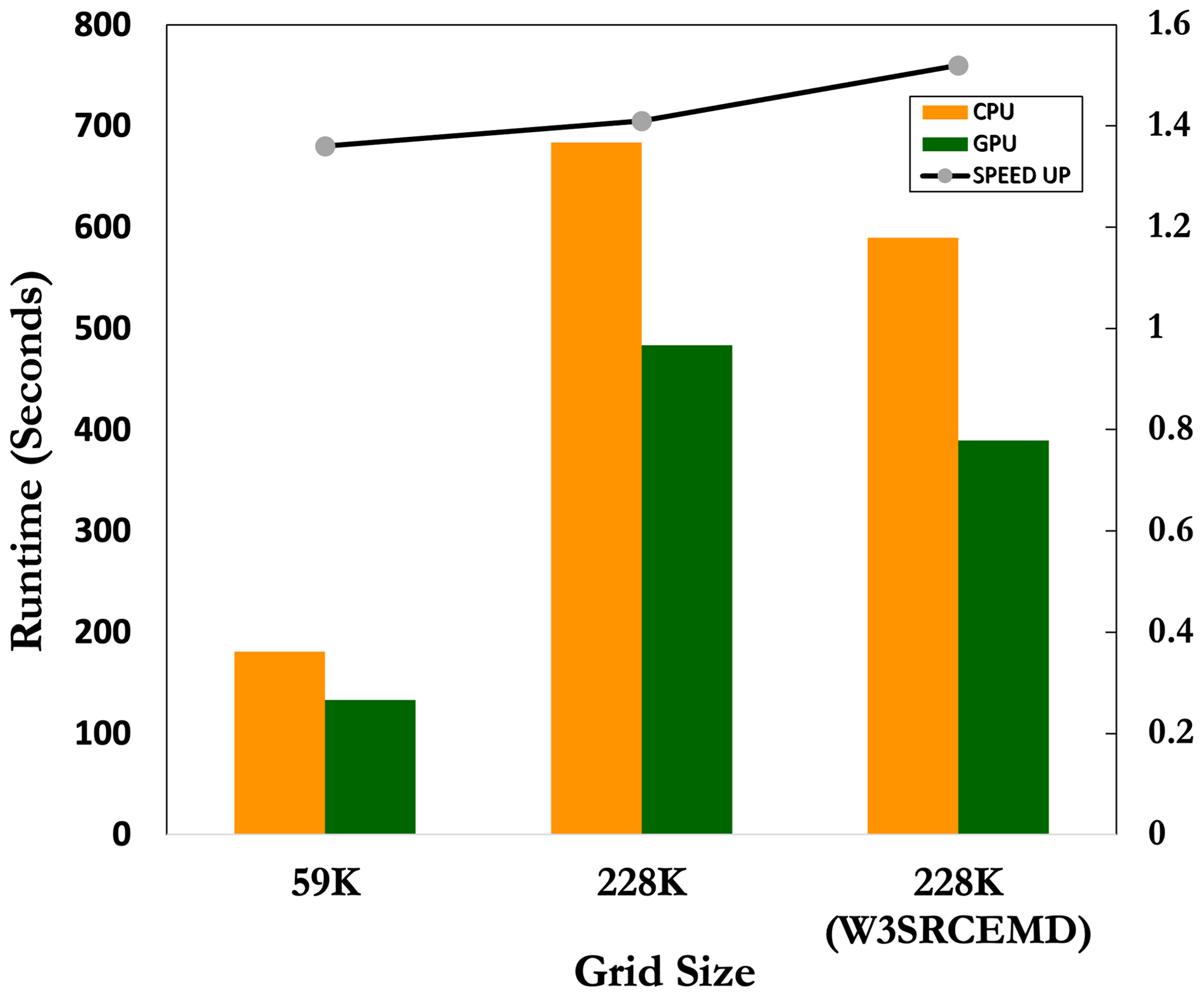
Figure 6 The runtime of WW3.cpu (orange) and WW3-W3SRCEMD.gpu (green) for 42 CPU cores and 7 MPI ranks per GPU on a Summit node with 59K and 228K meshes. The right-hand bar chart shows the runtimes for only the GPU-accelerated subroutine, W3SRCEMD, on a 228K grid size. The black line represents the speedup of WW3-W3SRCEMD.gpu over WW3.cpu.

Table 3 Node baseline comparison runtime (seconds) with different MPI ranks per GPU configuration on a Summit node. The numbers in square brackets are the speedup relative to the whole CPU on a Summit node (42 MPI ranks). In the last row, we present the speedups and simulation times when comparing only the GPU-accelerated subroutine, W3SRCEMD.

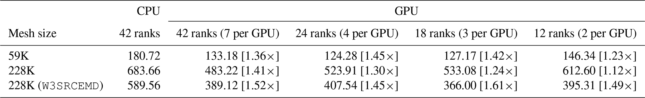
Table 4 The speedup of multiple nodes for the 228K mesh size on Summit. We used all 42 CPU cores and 6 GPU on each node with a configuration of 7 MPI ranks per GPU.

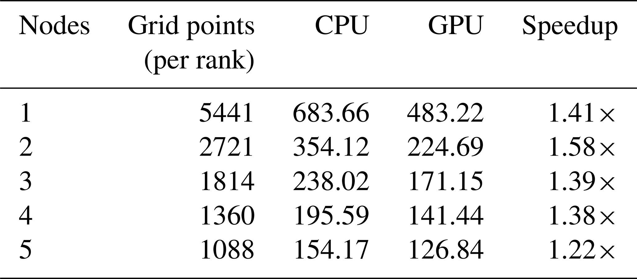
Table 4 shows the results of scaling the 228K mesh size over multiple nodes. We used the full GPU configuration here by launching seven MPI ranks on each GPU. In the results, it can be seen that the speedup is relatively uniform across multiple nodes. Likewise, as the number of grid points per MPI rank decreases with increasing nodes, the speedup gradually decreases due to reduced GPU utilization. However, the speedup is always the highest whenever the number of grid points per MPI rank is ∼ around 2500, e.g., the speedup of 2 nodes in Table 4 for 228K and the speedup of 24 MPI ranks for the 59K mesh in Table 3. This is most likely due to the tail effect – load imbalance between SMs. Based on our kernel launch configuration, 64 register and a 32 block size, the number of possible blocks per SM is limited to 32. With 80 SMs on a V100 GPU, the maximum total number of blocks (gangs, i.e., grid points) that could be executed simultaneously is 80×32 (2560).

All previous speedups are based on the whole WW3 code. However, only W3SRCEMD is accelerated on the GPU, whereas the rest of the code is run on the CPU. Thus, when comparing 24 MPI ranks in the GPU configuration with the 42 CPU cores, 24 MPI ranks are being used for the CPU section of WW3-W3SRCEMD.gpu against 42 MPI ranks for the WW3.cpu. Therefore, it is necessary to also consider only the speedup of W3SRCEMD on the GPU over the CPU. The last row of Table 3 (also Fig. 6) shows the runtimes and the achieved speedup of the W3SRCEMD subroutine for a 288K mesh size on a Summit node. In comparison with the speedup based on the whole WW3 code, the W3SRCEMD speedup increases for all configurations with a maximum speedup of 1.61×.

3.4 W3SRCEMD roofline plot

The roofline model helps us understand the trade-off between data movement and computation, so we can find out what is limiting our code and how close we are to it. The roofline (Fig. 8) indicates that, as expected from a memory-intensive model, the kernel is limited by the data transfer bandwidth between the CPU and the GPU. Most of the kernel's time is spent executing memory (load/store) instructions. It is worth mentioning that the device achieved a compute throughput and a memory bandwidth that are both below 40 % of its peak performance. Therefore, it appears that, while the computation is waiting for the GPU to provide required data, the GPU is waiting for the CPU to transfer data. Similarly, the roofline shows that the kernel memory bandwidth is approximately equal to the NVLink bandwidth. Thus, the W3SRCEMD kernel is limited by the bandwidth between the CPU and the GPU memory.

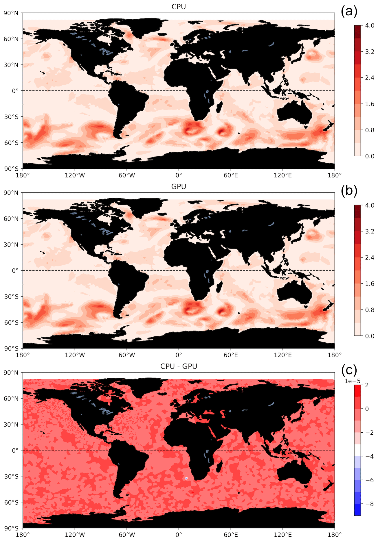
Figure 7 The average of WW3.cpu (a) and WW3-W3SRCEMD.gpu (b) last 2 h simulations and their differences (c) for significant wave height.

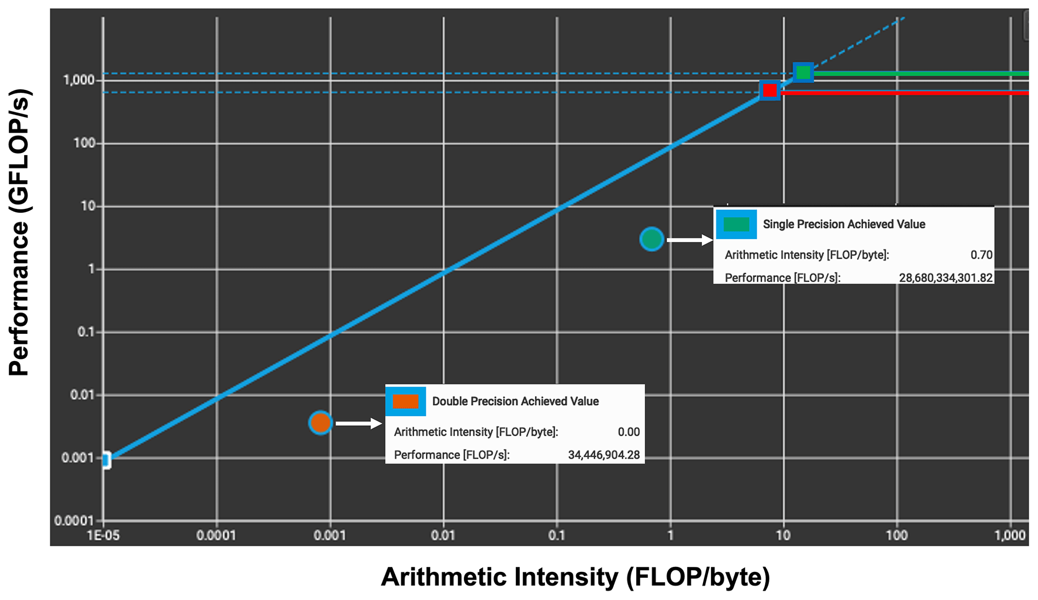
Figure 8 Roofline model for the W3SRCEMD kernel from NVIDIA Nsight Compute. The red and green dots are the double- and single-precision values, respectively.

The kernel also has a very low arithmetic intensity for both single- and double-precision floating-point (Fig. 8) computations, performing only very few flops for every double and integer loaded from dynamic random access memory (DRAM). Arithmetic intensity is a measure of floating-point operations (FLOPs) performed relative to the amount of memory accesses in bytes that are needed for those operations. For our 5 h simulation, the kernel is being launched 21 times; therefore, there are 42 data movements between the host and the device for nonconstant variables. Unfortunately, the large arrays need to be updated on both the device and host at each time step. As an example, VA, the spectra storage array, is approximately 5 GB (20 GB) for a spatial mesh size of 59 000 (228 000) and a spectral resolution of 50×36. In summary, the W3SRCE subroutine is simply too big and complicated to be ported efficiently using OpenACC routine directives and, therefore, requires significant refactoring.

4 Conclusions

Climate science is increasingly moving towards higher-spatial-resolution models and additional components to better simulate previously parameterized or excluded processes. In recent decades, the use of GPUs to accelerate scientific problems has increased significantly due to the emergence of supercomputers with heterogeneous architectures.

Wind-generated waves play an important role in modifying physical processes at the atmosphere–ocean interface. They have generally been excluded from most coupled Earth system models, partly due to the high computational cost of modeling them. However, the Energy Exascale Earth System Model (E3SM) project seeks to include a wave model (WW3), and introducing WW3 to E3SM would increase the computational time and usage of resources.

In this study, we identified and accelerated the computationally intensive section of WW3 on a GPU using OpenACC. Using the Valgrind and Callgrind tools, we found that the source term subroutine, W3SRCEMD, consumes 78 % of the execution time. The W3SRCEMD subroutine has no neighboring grid point dependencies and is, therefore, well suited for implementation on a GPU. Using two different computational platforms, Kodiak with four P100 GPUs and Summit with six V100 GPUs on each node, we performed 5 h simulation experiments using two global unstructured meshes with 59 072 and 228 540 nodes. On average, running W3SRCEMD by offloading one MPI per GPU gives an approximate 4× (2×) speedup over the CPU version on Summit (Kodiak). Via a fair comparison, using all 42 CPU cores and 6 GPUs on a Summit node, a speedup of 1.4× was achieved using 7 MPI ranks per GPU. However, the GPU speedup over the 42 CPU cores remains relatively unchanged (∼ 1.3×), even when using 4 MPI ranks per GPU (24 ranks in total) and 3 MPI ranks per GPU (18 ranks in total). The GPU performance is heavily affected by the data transfer bandwidth between the CPU and the GPU. The large number of local scalars and arrays within the W3SRCEMD subroutine and the huge amount of memory required to run WW3 is currently hurting the GPU utilization and, thus, the achievable speedup. Too many constants in WW3 occupy the register (fast memory) and then spill over to the L1 and L2 caches or the GPU global memory. To increase the GPU performance, the grid loop counter within W3WAVEMD must be pushed into the W3SRCEMD, thereby moving the gang-level parallelization into W3SRCEMD. This requires major code refactoring, starting with modification of WW3 data structures. There are other parts of the WW3 code that can be ported to GPU, such as spatial and spectral propagation.

Coupling the CESM with WW3 at low resolution, Li et al. (2016) found a 36 % and 28 % increase in computational cost for ocean-wave-only and fully coupled simulations when running WW3 on a $\mathrm{3.2}{}^{\circ }\times \mathrm{4}{}^{\circ }$ latitude–longitude grid with 25 frequency and 24 directional bins with a 3^∘ resolution ocean model and T31 atmosphere. Likewise, in a one-way coupling of WW3 to the E3SM atmospheric component, WW3 increases the number of processors by ∼ 35 % and its runtime is 44 % longer than the ocean model. From our first attempt at GPU-based spectral wave modeling, the runtime decreased by 35 %–40 % and resource usage decreased by 40 %–55 %. Thus, leveraging heterogeneous architectures reduces the amount of time and resources required to include WW3 in global climate models. It is important to note that WW3 will become a bottleneck as the ocean and atmosphere models in E3SM move towards heterogeneous architectures. Consequently, WW3 needs huge refactoring to take advantage of GPU capabilities and be fully prepared for the Exascale regime.

After refactoring the WW3 code, we also need to investigate how different WW3 setups (grid parallelization method, source term switches, propagation schemes, etc.) affect GPU performance. The performance of GPU-accelerated WW3 using OpenMP should also be considered for future work. The success of this work has laid the foundation for future work in global spectral wave modeling, and it is also a major step toward expanding E3SM's capability to run with waves on heterogeneous architectures in the near future.