the Creative Commons Attribution 4.0 License.
the Creative Commons Attribution 4.0 License.
 | 27 Feb 2023
Incorporation of aerosol into the COSPv2 satellite lidar simulator for climate model evaluation
Marine Bonazzola
Hélène Chepfer
Po-Lun Ma
Johannes Quaas
David M. Winker
Artem Feofilov
Nick Schutgens
Atmospheric aerosol has substantial impacts on climate, air quality and biogeochemical cycles, and its concentrations are highly variable in space and time. A key variability to evaluate within models that simulate aerosol is the vertical distribution, which influences atmospheric heating profiles and aerosol–cloud interactions, to help constrain aerosol residence time and to better represent the magnitude of simulated impacts. To ensure a consistent comparison between modeled and observed vertical distribution of aerosol, we implemented an aerosol lidar simulator within the Cloud Feedback Model Intercomparison Project (CFMIP) Observation Simulator Package version 2 (COSPv2). We assessed the attenuated total backscattered (ATB) signal and the backscatter ratios (SRs) at 532 nm in the U.S. Department of Energy's Energy Exascale Earth System Model version 1 (E3SMv1). The simulator performs the computations at the same vertical resolution as the Cloud-Aerosol Lidar with Orthogonal Polarization (CALIOP), making use of aerosol optics from the E3SMv1 model as inputs and assuming that aerosol is uniformly distributed horizontally within each model grid box. The simulator applies a cloud masking and an aerosol detection threshold to obtain the ATB and SR profiles that would be observed above clouds by CALIOP with its aerosol detection capability. Our analysis shows that the aerosol distribution simulated at a seasonal timescale is generally in good agreement with observations. Over the Southern Ocean, however, the model does not produce the SR maximum as observed in the real world. Comparison between clear-sky and all-sky SRs shows little differences, indicating that the cloud screening by potentially incorrect model clouds does not affect the mean aerosol signal averaged over a season. This indicates that the differences between observed and simulated SR values are due not to sampling errors, but to deficiencies in the representation of aerosol in models. Finally, we highlight the need for future applications of lidar observations at multiple wavelengths to provide insights into aerosol properties and distribution and their representation in Earth system models.
- Article
(4128 KB) - Full-text XML
- BibTeX
- EndNote


The role of aerosol in the Earth system has been recognized as a major source of uncertainty for decades. Aerosol has significant impacts on the climate system, as well as on weather and air quality, and Earth's biogeochemical cycles (Szopa et al., 2021). They modulate the Earth's energy budget via aerosol–radiation and aerosol–cloud interactions, exerting radiative forcings to the climate system (Forster et al., 2021). They also affect the Earth's water cycle by changing clouds and precipitation characteristics (Douville et al., 2021). Due to its short lifetime (up to several days in the troposphere) compared to long-lived greenhouse gases, aerosol is highly variable in space and time. Obtaining appropriate information about the spatiotemporal distribution of aerosol from satellite measurements remains a key challenge (Constantino and Bréon, 2013).
Passive satellite measurements have been used to study column-integrated properties of aerosol, but they are not suited for the vertical distribution of aerosol. Nevertheless, aerosol vertical distribution is critical when it comes to aerosol–radiation interactions (Zarzycki and Bond, 2010). This in particular applies to the adjustments to aerosol–radiation interactions or semi-direct effects, where the vertical alignment of clouds and aerosol is crucial (Koch and Del Genio, 2010). Aerosol vertical distribution also affects aerosol lifetime (e.g. Keating and Zuber, 2007) and aerosol–cloud interactions (e.g. Waquet et al., 2009; Stier, 2016; Quaas et al., 2020).
Spaceborne lidars fill this gap by providing detailed information about the vertical distribution of aerosol. This is particularly useful for studying long-range transport of smoke or dust in the free troposphere and stratosphere and for studying the interactions between aerosol and ice clouds in the upper troposphere, because the vertically integrated aerosol quantities retrieved from passive sensors are mostly about aerosol in the planetary boundary layer. Furthermore, space lidars can retrieve aerosol in regions where the surface is reflective, such as the polar regions and desert, while passive satellite instruments only have limited capabilities retrieving aerosol in those conditions. Over the last decade, the aerosol profiles collected by space lidars (Winker et al., 2013) have contributed to progress on a variety of aerosol research questions (Koffi et al., 2012, 2016; Tian et al., 2017; Ratnam et al., 2021). More advanced comparisons between model and lidar observations have demonstrated the value of using a lidar aerosol simulator to ensure consistent comparisons between the modeled aerosol and the observed aerosol (Ma et al., 2018; Hodzic et al., 2004; Watson-Parris et al., 2018). In parallel, the cloud community has developed satellite simulators to establish a closer bridge between observed and modeled clouds and facilitate the use of space-based data by the model community for a variety of topics such as evaluating the model physics, studying climate feedbacks, and inter-comparing several models in a consistent way over short-term and long-term simulations (Konsta et al., 2016; Chepfer et al., 2018). In particular, the active sensor satellite simulators developed for lidars and radars have been proven to be useful tools to properly take into account the limits of observations (e.g. cloud masking, signal-to-noise ratio, sub-gridding) when comparing observations and models (e.g. Ma et al., 2018).
These studies point to the potential for satellite lidars to provide important constraints for the aerosol distributions in climate models, which are of benefit to a range of different configurations. There is now a 15-year-record of the spaceborne Cloud-Aerosol Lidar with Orthogonal Polarization (CALIOP) on the Cloud-Aerosol Lidar and Infrared Pathfinder Satellite Observation (CALIPSO) satellite (2006–2020). In evaluating the simulated vertical aerosol distribution in nudged simulations where, for example, winds are relaxed towards reanalyses, these measurements can provide important observational constraints to improve transport and removal processes in models. On the other hand, using observational constraints together with a climatology statistic approach of simulations with prescribed sea surface temperature (SST) can be beneficial to account for circulation feedbacks to aerosol forcing. Indeed, while the transport by large-scale circulation determines the geographical patterns of aerosol forcing, this aerosol forcing also impacts large-scale circulation (Kim et al., 2007). These mechanisms can be studied by making use of aerosol optical depths (AODs) retrieved by the Moderate Resolution Imaging Spectroradiometer (MODIS) or Visible Infrared Imaging Radiometer Suite (VIIRS). Finally, long-term (100 years) simulations of the coupled ocean–atmosphere system (control and Representative Concentration Pathway 8.5, RCP8.5, type simulations) can help to understand the role of aerosol in the context of climate change.
The lidar simulator translates the vertical profiles of aerosol extinction and backscatter coefficients computed by a model into vertical profiles of the two key variables retrieved by a lidar: the attenuated total backscatter (ATB) and the backscatter ratio (SR). These two lidar variables are derived online within the model to account for the two-way attenuation within the light's transmittance along its path from the laser to the scattering object, as well as the return path back to the detector. The calculations also account for the molecular backscatter (i.e. Rayleigh backscatter), calculated from the model's air temperature and pressure profiles. Furthermore, the model is sampled on the satellite orbital path, the fully overcast cases are masked out to take account of the impossibility for a space lidar to observe aerosol below optically thick clouds, and only the signal above the instrumental noise is retained.
We incorporate modules included in previously developed simulators (Ma et al., 2018; Vuolo et al., 2009; Hodzic et al., 2004) into the community tool Cloud Feedback Model Intercomparison Project (CFMIP) Observation Simulator Package version 2 (COSPv2) to create a simple base on which each group can build up its own analysis. The goal is to facilitate the comparison between general circulation models (GCMs) and space lidar aerosol data. Besides CALIPSO operating at 532 and 1064 nm, the Atmospheric Lidar (ATLID) instrument of the EarthCARE mission is expected to become operational in 2023. In synergy with other instruments, it will provide vertical profiles of aerosol and thin clouds, operating at 355 nm with a high-spectral-resolution (HSR) receiver and depolarization channel. Moreover another HSR Lidar operating at 532 and 1064 nm is expected to be launched in the future. The COSPv2 lidar simulator will thus be a useful tool for the exploitation of these new datasets and the comparison with GCMs of several modeling groups.
We have chosen to implement the lidar aerosol simulator within the COSPv2 software package to leverage all the simulator capabilities available in COSPv2. Moreover, COSPv2 is already implemented in several GCMs (Swales et al., 2018), so the addition of the aerosol lidar simulator module should only require a small amount of effort for the modeling groups.
The aerosol simulator described in this section mimics the aerosol observations that would be observed by a space lidar overflying the atmosphere simulated by the model (Fig. 1). Hereafter, we first define the usual aerosol variables (specifically, the attenuated total backscattered signal ATB and the backscatter ratio SR). Then, we describe the procedure of the lidar aerosol simulator. Finally, we discuss its implementation and its main differences with the cloud lidar simulator.
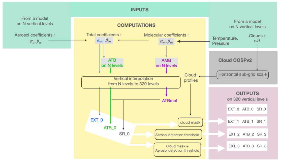
Figure 1Schematic of the lidar aerosol COSPv2 simulator. See Table 1 for the correspondence between the names of the variables in the code and in the present paper.
2.1 Definitions
As defined by Stromatas et al. (2012), the attenuated total backscattered signal (in m−1 sr−1) represents the signal backscattered towards the lidar by aerosol and molecules and attenuated along its path by aerosol and molecules in a cloud-free atmosphere. The ATB is integrated vertically from the surface to the top of the atmosphere (TOA):
where βm and βa are the molecule and aerosol 180∘ backscatter profiles (in m−1 sr−1), respectively, and αm and αa are the extinction coefficients for molecules and aerosol (in m−1), respectively. The 180∘ Rayleigh/molecular backscatter coefficient depends on temperature (in K), pressure (in Pa) and on the wavelength λ (in µm):
where k is the Boltzmann constant ( J K−1). The extinction coefficient by molecules can be simply expressed as
(Stromatas et al., 2012). The 180∘ backscatter and extinction coefficients for aerosol depend on the microphysical properties (size distribution) and chemical composition of the particles, the latter determining its refraction index. To highlight aerosol in an atmospheric layer versus molecular background, one often uses the backscatter ratio (SR). The definition of SR used in CALIPSO products (e.g. Chepfer et al., 2008, 2013) is
where AMB is the attenuated molecular backscatter signal in the absence of aerosol:
Therefore, SR=1 indicates the absence of aerosol, where the backscatter signal is from gaseous molecules only.
2.2 Concept
The GCM provides pressure, temperature and cloud fraction at each level and for each latitude–longitude grid cell. When the GCM includes an interactive aerosol module, it also provides on this 3D grid the optical properties of aerosol at a given wavelength. The simulated aerosol optical properties and distribution depend on the aerosol parameterization in the GCM. The aerosol optics diagnostics in GCMs vary, with some models computing single-wavelength extinction and 180∘ backscatter, whilst others calculate only the waveband-integrated aerosol optical properties (i.e. extinction, absorption and phase function). In the latter case, the modeling centers will need to implement additional aerosol optics diagnostics to convert these optical properties into the aerosol extinction and 180∘ backscatter coefficients in order to use the lidar simulator. These coefficients must be defined monochromatically, i.e. at specific wavelengths, 532 and 1064 nm for CALIPSO/CALIOP, with these being standard wavelengths for most GCMs. Coefficients defined at other wavelengths, such as 355 nm for EarthCARE ATLID, could also be added as additional diagnostics.
In the steps listed below, it is assumed that the process applies to a vertical profile and that it is repeated for all longitude–latitude grid cells and for each instantaneous model output. In this study, the model writes out at 01:30 and 13:30 local time, corresponding to the CALIPSO overpass time.
-
Construct sub-grids. The ACTSIM procedure already implemented in COSP calculates the αM(z), βm(z) and AMB(z) vertical profiles using the GCM pressure and temperature profiles, according to the equations of Sect. 2.1. The GCM vertical profile of cloud fraction is also passed to the Subgrid Cloud Overlap Profile Sampler (SCOPS) (Klein and Jakob, 1999) procedure in COSPv2 to generate sub-grid columns within a grid cell in accordance with the simulated cloud fraction and the vertical overlap assumption.
-
Compute ATB and SR. The ATB and SR profiles are computed at model levels. These variables are calculated according to the equations of Sect. 2.1, using the input variables αa and βa and the variables αmβm and AMB calculated in step 1. Because the GCM does not consider sub-grid variability of aerosols, we compute the ATB and SR for each grid cell.
-
Vertical regridding. The total extinction (αa+αm), ATB and SR profiles are vertically re-gridded over a standard vertical grid having N equidistant levels to obtain profiles of total extinction (EXT_initial), attenuated total backscatter (ATB_initial) and backscatter ratio (SR_initial) at the vertical resolution of the space lidar observations that would be observed in absence of instrumental noise. For consistent comparison with CALIPSO observations, N is set to 320 levels so that each level is 60 m thick from the surface to 19.14 km of altitude. We design the code to allow N to be set by users so that it can be easily adapted for other lidars. For example, the vertical resolution of EarthCARE ATLID is 100 m, so N will need to be set to 192 for the simulator to operate between the surface and 19.1 km above ground level.
-
Apply aerosol detection thresholds. The aerosol detection thresholds, based on the actual space lidar capability (above instrumental noise), are applied to the EXT_initial, ATB_initial and SR_initial profiles, in order to get the profiles of total extinction (EXT_detectable), attenuated total backscatter (ATB_detectable) and backscatter ratio (SR_detectable) that would be observed by a space lidar overflying the atmosphere simulated by the model in absence of clouds. This takes into account the limited capability to detect aerosol when the signal-to-noise ratio (SNR) is too low for CALIPSO. The aerosol detection threshold considered in this study is SR = 1.2, which is different from the previous study that considered the detection threshold as a function of height (Ma et al., 2018), but we designed the code to be flexible so that it can be easily adapted for sensitivity studies or for future space lidars that have a different SNR.
-
Apply cloud masking. The cloud masking is applied to the initial profiles EXT_initial, ATB_initial and SR_initial to get the total extinction (EXT_masked), attenuated total backscatter (ATB_masked) and backscatter ratio (SR_masked) profiles that would be observed above clouds by a space lidar with a perfect aerosol detection capability (no instrumental noise). This takes into account the fact that a space lidar is unable to observe aerosol below optically thick clouds (with optical depth larger than 3–5) where the laser beam is fully attenuated. To simulate this cloud masking effect, the cloud masking in the simulator is built from the modeled clouds (not the actual clouds) as it would be seen by a space lidar. We take the cloud lidar simulator output called cloud fraction profiles (CF3D). When scanning each grid point from the TOA to the surface, the first altitude level where CF3D = 1 is called “z_bottom” and all aerosol-related output values at that altitude and below are set to Fill_value.
-
Combine all factors. The cloud masking (step 5) and aerosol detection thresholds (step 4) are applied to the initial profiles (EXT_initial, ATB_initial and SR_initial) to get the total extinction (EXT_observable), the attenuated total backscatter (ATB_observable) and backscatter ratio (SR_observable) profiles that would be observed above clouds by a space lidar with actual aerosol detection capability.
Note that in the code, the variables have different names than in this paper. Table 1 establishes the correspondence between the names of the variables in this text and in the code.
Table 1Translations between the name of the variables in the text and in the code. For example, EXT_initial in the paper corresponds to EXT0 in the code.

2.3 Differences between the CALIPSO aerosol and cloud simulators
The aerosol lidar simulator is implemented within the COSPv2 infrastructure, which has been optimized for computational performance so that it can be used for long climate simulations when needed. COSPv2 already contains a cloud lidar simulator from which several routines are used within the aerosol lidar simulator (Chepfer et al., 2008; Cesana and Chepfer, 2012, 2013; Guzman et al., 2017; Reverdy et al., 2015). The main differences between the aerosol lidar simulator presented in this paper and the cloud lidar simulator are described below.
-
The aerosol lidar simulator needs aerosol optics from the models as inputs (αa and βa profiles in each model grid box) because those optical properties are strongly dependent on aerosol size distribution and chemical composition. They depend on the aerosol parametrization in the GCM, and the size of aerosol is close to the lidar wavelength. By contrast, because cloud droplets are much larger than the lidar wavelength, cloud optical properties can be parameterized in a simpler way than aerosol, so COSPv2 can easily compute cloud optical properties from cloud microphysical properties.
-
Within the aerosol lidar simulator, the computations are performed in each grid box (with a typical grid spacing of 1∘), while the cloud simulator computations are performed at a sub-grid scale (typically 50 sub-grid boxes in a grid box). This is consistent with the assumptions in GCMs. While GCMs represent the sub-grid variability of clouds, aerosol is assumed to be homogeneous within a grid box. Therefore, the aerosol lidar simulator assumes that aerosol is uniformly distributed horizontally within a grid box while cloud simulators assume sub-grid variability according to SCOPS.
-
The aerosol lidar simulator uses a higher-resolution vertical grid than the cloud simulator: e.g. 320 vertical levels (typically 60 m) instead of 40 (typically 480 m). This is because the detailed vertical structure of aerosol is important for understanding aerosol mixing, transport and other physical processes, especially in the atmospheric boundary layer. To be consistent with the CALIOP aerosol data product, we use the same vertical resolution. Note that for clouds the vertical resolution used in CFMIP experiments (dz=480 m) results from a compromise between the wish to keep high horizontal resolution for sparse shallow clouds, the SNR of CALIOP data in daytime and the vertical resolution of CloudSat.
Users can choose to run the new aerosol simulator alone, the standard cloud simulators alone (default), or both aerosol and cloud simulators. These new features are controlled by two new keys in the user's configuration file in COSPv2 code. Users can set “lidar_aerosols” and “use_vgrid_aerosols” to true to invoke the aerosol simulator. The logical variable “use_obs_for_aerosols” must be set to “false” for now as it is reserved for future feature development. Lastly, users need to set the number of vertical levels for aerosol “nlvgrid_aerosols”, which is set to 320 by default as recommended by this study.
To facilitate fair comparisons between models and observations, we have created an observational dataset that is consistent with the simulator approach described in the previous section. The simulator outputs SR_observable and ATB_observable can be directly compared with the SR and ATB profiles above clouds observed by CALIOP. However, it should be noted that the total extinction profile (EXT_observable) cannot be observed directly by CALIOP, it is an output from the simulator that can only be used to interpret the difference between the observation and the model and simulator outputs.
We use the CALIOP L1.5 orbit file (NASA/LARC/SD/ASDC, 2019) dataset that contains cloud-screened ATB profiles at 532 nm with 60 m vertical resolution and 20 km along-track and 90 m cross-track horizontal resolution. The CALIOP L1.5 data are built from the native L1 CALIOP data ( km along-track horizontal resolution, 90 m cross-track horizontal resolution and 30 m vertical resolution), but a cloud-screening procedure is applied so that the L1.5 data only contain above-cloud measurements. The cloud screening is applied iteratively at different horizontal resolutions from up to 80 km. When clouds are detected at a vertical level, all the data below the cloudy level are marked as Fill_Value and all the cloud-free and above-cloud profiles are retained below the altitude of 8 km. Then, these cloud-free and above-cloud profiles are averaged horizontally over the along-track 20 km grid. Since each L1.5 20 km profile represents an averaged signal over the cloud-free profiles over 20 km, this dataset cannot be used to study the horizontal heterogeneity of aerosol with a spatial scale smaller than 20 km. Nevertheless, this dataset has the advantage of a much higher SNR than the original L1 profile ( km), which permits the use of a lower aerosol detection threshold in both observations and simulations, and is then able to detect optically thin aerosol layers at the 20 km spatial scale (Ma et al., 2018).
In this study, we created an example gridded data product from CALIPSO that is consistent with the GCM grid, so that the translation from the model to the simulator results can be more easily understood by the reader, in relation to how it can affect the interpretation of a comparison to the CALIOP observation profile. This dataset was created by averaging all the L1.5 ATB cloud-screened profiles over a 1∘ × 1∘ latitude–longitude grid at a given date. It is worth noting that since CALIPSO is a polar-orbiting satellite with a relatively narrow swath, the number of profiles at high latitudes is larger than that in the tropics, and that not all the grid boxes contain a satellite observation in any single day.
Similarly, we build the gridded product for SR from the orbit L1.5 ATB dataset. We first compute the AMB profiles – the signal that would be measured by the lidar in a cloud-free and aerosol-free atmosphere – at the 20 km along-track resolution and 60 m in the vertical from the pressure and temperature profiles from NASA Global Modeling and Assimilation Office (GMAO) that are included in the L1.5 data. We compute the SR profiles by dividing the L1.5 ATB with AMB. Finally, we average all the 20 km SR profiles over 1∘ × 1∘ grid boxes. Because the model SR profile is normalized against the model pressure and temperature profiles and the observed SR profile is normalized against the pressure and temperature from the GMAO reanalysis, comparing SR profiles between observations and models is more informative regarding aerosol distributions than ATB profiles which are subject to differences in atmospheric temperature and pressure as well.
In the upper troposphere where AMB and ATB values are low, the ATB profiles measured along the orbit have low signal-to-noise ratios, which leads to high values of SR, even at 1∘ × 1∘ resolution. To address this issue, we set ATB equal to AMB when ATB minus AMB is lower than 1 × 10⁻⁴ km−1 sr−1 and SR equal to 1 when SR is lower than 1.2. The threshold on AMB typically applies above 8 km. While this procedure removes the noise, it can also remove the signal from the tenuous aerosol layer (e.g. Watson-Parris et al., 2018). Both threshold values are relevant for night profiles, which are less noisy than daily ones. We thus focus in this study on profiles observed at night only, before and after the application of the AMB–SR thresholds. Note that the threshold on SR is parameterized in the aerosol simulator and can be easily adjusted to other values for various research and application purposes.
Finally, we generate daily and monthly average of the gridded data. This enables users to perform comparisons at three different spatiotemporal scales: (1) the instantaneous SR profiles at the resolution of 1∘ along track and 60 m in the vertical, (2) the 3D daily 1∘ × 1∘ gridded SR data with a 60 m vertical resolution, and (3) the 3D monthly 1∘ × 1∘ gridded SR data with a 60 m vertical resolution.

Figure 2Attenuated total backscatter profiles (km−1 sr−1) before noise filtering (a) and after noise filtering (c); backscatter ratio profiles before noise filtering (b) and after noise filtering (d); observed by CALIOP at 532 nm along the satellite orbit on 20 March 2008.
4.1 Orbit files
We consider the attenuated total backscatter profiles observed by CALIPSO at 532 nm along its trajectory on 20 March 2008 as an example to demonstrate the comparison using the aerosol simulator and show the impacts of the AMB–SR thresholds. These profiles, characterized by their latitude in Fig. 2a and c, show missing values below the clouds with sufficient optical thickness to fully attenuate the laser beam. Such clouds occur at very high altitudes within the tropics, making it impossible to retrieve significant signals below 17 km at some locations. In dry regions (e.g. between 10 and 30∘ N, 20 and 40∘ S), however, the absence of clouds allows the lidar to retrieve entire ATB profiles down to the surface. The attenuated total backscatter signal, which contains the molecular backscatter signal, shows a maximum near the surface, with a monotonic decrease as altitude increases. The SR profiles (Fig. 2b and d), being normalized by the molecular signal, filter out the contribution by air molecules and are thus more appropriate to retrieve aerosol concentrations. A large amount of SR values that were initially lower than 1 because of the instrument noise (Fig. 2b) are set to 1 by the application of the AMB–SR thresholds (Fig. 2d). In this particular orbit, two dense aerosol layers can be identified. One is in the polar region in the Northern Hemisphere between 10 and 12 km, and another one is in the lower troposphere at 30∘ S. CALIPSO also shows signals of thinner aerosol layers that are generally below 4 km.
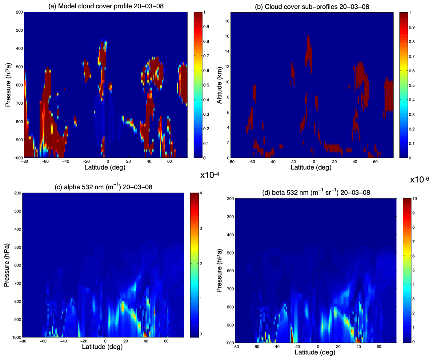
Figure 3(a) Vertical profiles of cloud fraction simulated by the E3SMv1 model along the satellite orbit on 20 March 2008; (b) same vertical profiles, defined by the COSPv2 simulator at the sub-grid scale and interpolated on 40 vertical levels; (c) aerosol extinction profiles (in m−1) and (d) aerosol backscatter coefficient profiles (in m−1 sr−1) calculated by E3SMv1 along the satellite orbit.
In Fig. 3, we show the results of the U.S. Department of Energy's Energy Exascale Earth System Model version 1 (E3SMv1) (Golaz et al., 2019) with improved calibration of cloud and sub-grid effects (Ma et al., 2022). The model is configured to run with prescribed SST and sea ice extent. The E3SM Atmosphere Model version 1 (EAMv1) (Rash et al., 2019) model outputs are used to compute the ATB and SR profiles that would be seen by the lidar along its trajectory on the same date (20 March 2008). The model horizontal winds are nudged towards Modern-Era Retrospective analysis for Research and Applications version 2 (MERRA-2) (Gelaro et al., 2017) reanalysis with a relaxation timescale of 6 h (Zhang et al., 2014; Ma et al., 2015). The simulated cloud vertical profiles (Fig. 3a) agree very well with the observations (Fig. 2), as high cloud fractions along the satellite trajectory coincide with the horizontal locations and altitudes of missing data in the observations.
The vertical profiles of cloud fractions of Fig. 3a are then defined at the horizontal sub-grid scale (with about 50 profiles being produced in each grid box), with values of cloud fraction being equal to 0 or 1 in each sub-grid box. Vertically, the cloud fractions are interpolated on 40 levels, defined by their altitude. The resulting sub-profiles are shown in Fig. 3b and are consistent with the model outputs of cloud cover of Fig. 3a.
Finally, the aerosol optical properties αa and βa calculated by the E3SMv1 model at 532 nm along the satellite trajectory are used as inputs to the COSPv2 simulator. These quantities are calculated by the E3SM model at a very high vertical resolution, where the layer thickness is about 25 m at the surface, about 90 m in the first 1.5 km above the ground level, and about 600 m between 1.5 and 10 km (Rasch et al., 2019; Xie et al., 2018). The aerosol extinction and backscatter profiles show a very high correlation, with largest values below 800 hPa (Fig. 3c and d).
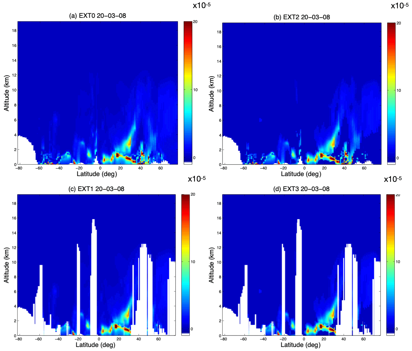
Figure 4Total extinction vertical profiles (m−1) defined on 320 levels and calculated by the COSPv2 simulator along the satellite orbit on 20 March 2008: (a) initial profiles; (b) profiles with the instrument aerosol detection threshold; (c) cloud-screened profiles; (d) cloud-screened profiles with the aerosol detection threshold applied.
The αa profiles are then interpolated vertically on the 320 altitude levels to produce the EXT_initial variable (Fig. 4a). The differences between the EXT_initial and EXT_detectable fields (Fig. 4b) illustrate the effect of applying the instrument aerosol detection threshold. In the EXT_detectable field, the values of the extinction coefficients that are lower than that threshold are set to zero. The extinction profiles thus appear less noisy in the middle troposphere (for example around 6 km at 20∘ S), whereas they remain similar in the lower troposphere. Finally, the EXT_masked field (Fig. 4c) shows the extinction profiles when the cloud screening is applied, and the EXT_observable field (Fig. 4d) combines the cloud screening and the aerosol detection threshold.
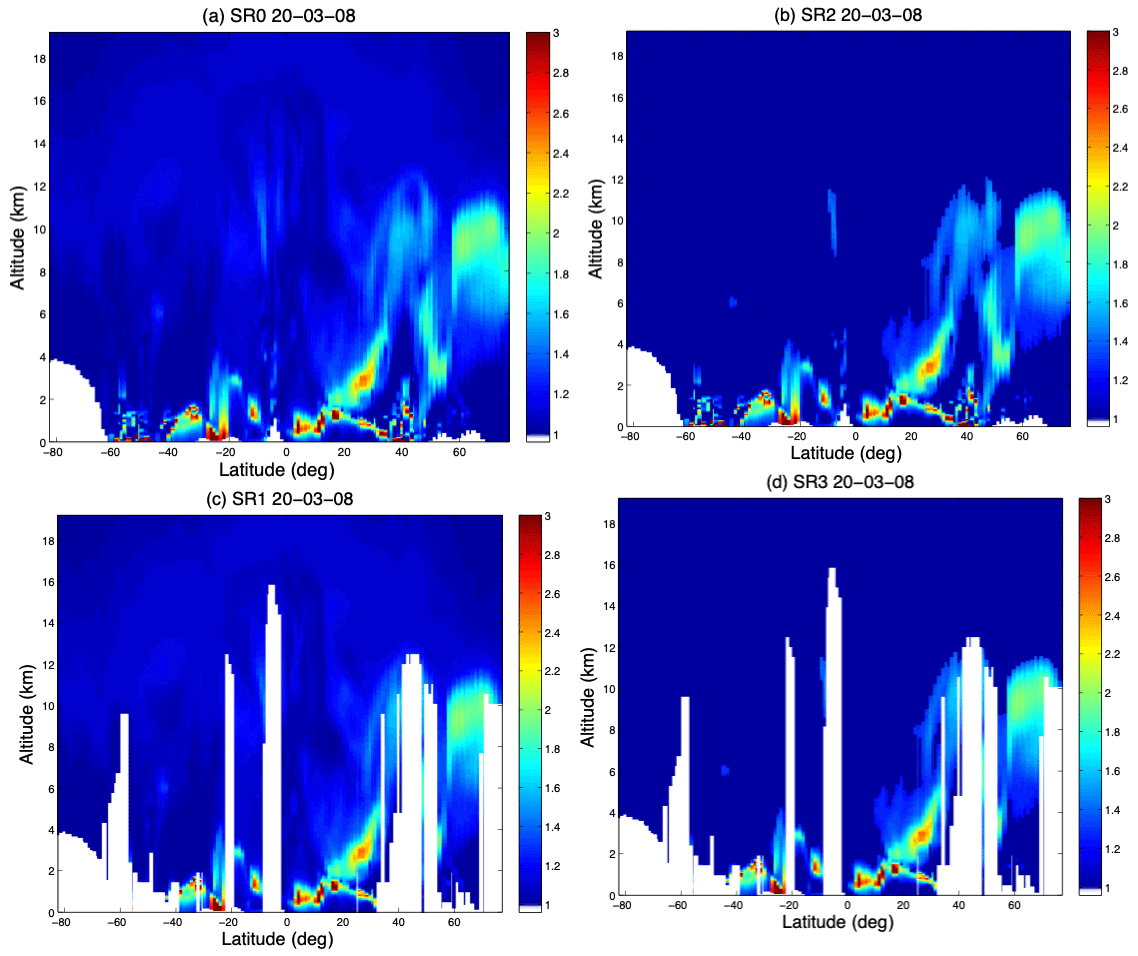
Figure 5Backscatter ratio vertical profiles defined on 320 levels and calculated by the COSPv2 simulator along the satellite orbit on 20 March 2008: (a) initial profiles; (b) profiles with the instrument aerosol detection threshold; (c) cloud-screened profiles; (d) cloud-screened profiles with the aerosol detection threshold applied.
The resulting SR profiles computed by the COSPv2 simulator are shown in Fig. 5. The obtained SR values, going up to 3 in maximum regions, agree well with the observations. South of 20∘ N, the signal above the detection threshold (Fig. 5b) is found below the altitude of 4 km, but north of 20∘ N, the aerosol plume extends vertically, and a significant signal is found at altitudes as high as 12 km, in good agreement with the observations (Fig. 2b).

Figure 6(a) Difference between model SR_masked and CALIOP data before data processing; (b) difference between model SR_observable and CALIOP data after data processing (see text for details) along the satellite orbit on 20 March 2008.
Figure 6 shows the impacts of the AMB–SR thresholds on the comparison between the simulated and observed SR profiles. In Fig. 6a, we show the differences between the SR_masked field (with cloud screening only) and CALIOP profiles before applying the AMB–SR thresholds. In the upper troposphere, the instrument noise induces differences in absolute value that sometimes exceed 0.4. In Fig. 6b, the differences between the SR_observable field (with cloud screening and aerosol detection threshold) and the CALIOP profiles after applying the AMB–SR thresholds become close to zero in the upper troposphere. In this comparison, we find that the E3SMv1 model underestimates the aerosol concentrations near the surface around 30∘ S but overestimates the concentrations in the aerosol plume north of 20∘ N between 1 and 9 km.
4.2 Global statistics
To have an overview of the aerosol distribution at the seasonal timescale, we average the observed and simulated ATB and SR profiles over 3 months: March, April and May (MAM) 2008. As aforementioned, the thresholds on AMB and SR are applied to observations. The profiles are further averaged over all longitudes for each 1∘ latitude bin and are represented in Fig. 7. The attenuated total backscatter signal, as the molecular backscatter signal (not shown), shows a decrease with altitude in the lower troposphere. The SR ratio, directly depending on aerosol concentrations, shows maxima reaching the value of 3 in the 2 km layer above the surface, indicating a very dense aerosol layer in the boundary layer. The ratios are especially large at 10∘ N and between 40 and 60∘ S, which can be attributed to the presence of dust and sea spray aerosol. At 10∘ N, dust is the predominant component of aerosol over northern Africa, the Arabian Peninsula and western China (Yu et al., 2010). Between 40 and 60∘ S, the main aerosol contribution during the MAM season is sea spray, as biomass burning over South America and southern Africa occurs mainly between June and November. The maximum between 40 and 60∘ S also appears within the first kilometer above the surface on zonal-mean 532 nm aerosol extinction profiles retrieved from CALIOP over the whole year during nighttime by Winker et al. (2013). The vertical extension of the aerosol plume seems to be largest in the Northern Hemisphere, where convection is the most active in MAM, whereas it is limited to the top of the boundary layer in the Southern Hemisphere, consistently with the scale heights retrieved by Yu et al. (2010).

Figure 7(a) Attenuated total backscatter profiles (km−1 sr−1) and backscatter ratio profiles (b) observed by CALIOP at 532 nm at night and averaged over longitudes and time during MAM 2008.
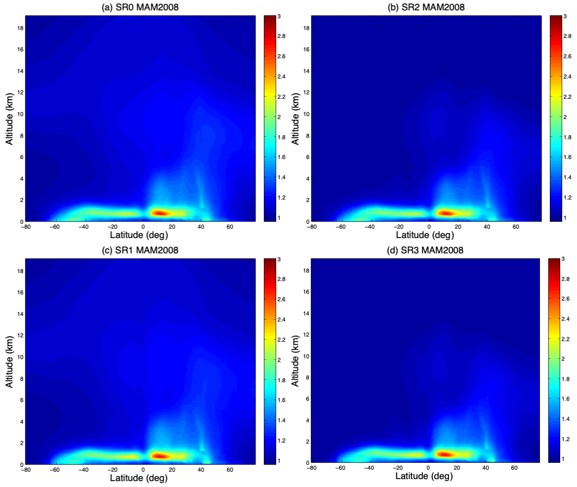
Figure 8SR profiles simulated by E3SMv1 at 532 nm and averaged over longitudes and time during MAM 2008: (a) initial profiles; (b) profiles with the instrument aerosol detection threshold; (c) cloud-screened profiles; (d) cloud-screened profiles with the aerosol detection threshold applied.
The simulated SR_observable profiles computed for the same period by the COSPv2 simulator are shown in Fig. 8d. The maximum at 10∘ N is well reproduced, but the maximum in the Southern Hemisphere does not appear, which might be due to an inaccurate simulation of sea spray aerosol in the model at this time and location. As in the observations, the aerosol plume shows a larger vertical extension in the Northern Hemisphere than in the Southern Hemisphere, which validates the convective transport of aerosol in the model. Yu et al. (2010) raised the issue that the convective transport of aerosol could not be well observed by CALIOP because it is not possible to retrieve aerosol in the presence of thick convective clouds. However, the comparison between the SR_initial (Fig. 8a) and SR_masked fields (Fig. 8c) shows minor differences, indicating that, at least in this particular model simulation, cloud screening does not affect dramatically the mean aerosol concentrations and does not modify significantly the amount of aerosol transported upward.
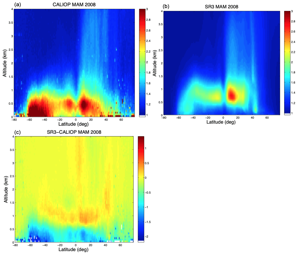
Figure 9(a) CALIOP SR after data processing (see text for details); (b) model SR_observable; (c) difference between model SR_observable and CALIOP SR. All fields are shown between 0 and 4 km and are averaged over all longitudes and time during MAM 2008.
Finally, we compare the simulated and observed SR values to identify model biases. Figure 9 shows the differences between the SR_observable profiles and the CALIOP SR profiles after the application of the AMB–SR thresholds (see Sect. 3) in the first 4 km above the surface. The SR maxima are underestimated by 1 to 1.5 in the model from the surface to 500–800 m and are slightly overestimated above this level up to 1.5–1.8 km. The underestimation of SR in the surface layer corresponds to a relative model error on the aerosol optical depth of approximately 50 %. This vertical distribution bias revealed by the simulator could have several causes that need to be investigated further, such as overly efficient vertical mixing or incorrect wet scavenging in the E3SMv1 model.
4.3 Validity of the comparison between CALIOP data and simulator outputs
A cause of the discrepancy between simulated SR_observable fields and SR fields retrieved from CALIOP observations can be the differences between model and observed clouds. For those two fields corresponding to cloud-free conditions only, the differences in the occurrences of cloud-free scenes in the model and observations can affect the sampling of aerosol concentrations. If those aerosol plumes show a large spatiotemporal variability, differences in sampling can induce differences in the seasonal or zonal-mean concentrations and thus in the mean SR.
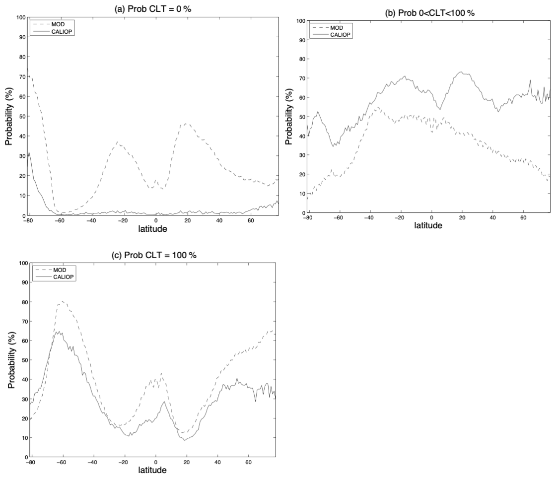
Figure 10Probabilities of (a) cloud-free, (b) partially cloud covered, and (c) totally cloud covered 1∘ × 1∘ horizontal grid cells as a function of latitude, during the MAM period (nighttime), in CALIOP and E3SMv1.
To compare the sampling induced by the cloud screening in E3SMv1 and in CALIOP, we consider the probability of having cloud-free conditions during the night at a daily scale in 1∘ × 1∘ horizontal grid cells at a given latitude, during the MAM period (Fig. 10a). In the observations, the total cloud cover (CLT) is estimated in the 532 nm channel of CALIOP. The probability for cloud-free conditions (CLT = 0 %) at nighttime is extremely low in CALIOP for all latitudes, except for polar regions that are dry and less cloudy than the rest of the globe (especially over land). The cloud-free probability is much higher in E3SMv1, with a maximum value of 70 % in the Southern Hemisphere polar region and about 40 % and 50 % at 25∘ S and 25∘ N, respectively.
However, the cloud-free grid cells are not the only ones to be sampled for the estimation of the mean SR. SR can still be obtained in grid cells with partial cloud cover (0 % < CLT < 100 %), as the SR will be computed in the clear-sky sub-columns of the considered grid cell in E3SMv1 and retrieved in the cloud-free pixels belonging to the grid cell by CALIOP. Making the reasonable assumption that aerosol concentrations are homogeneous within the 1∘ × 1∘ grid, this local estimation of SR can be considered to be representative of the whole grid cell.
The probability of partially covered grid cells (shown in Fig. 10b) is generally higher in CALIOP observations that in the E3SMv1 model. In CALIOP, the probability shows two maxima of about 70 % in the subtropical regions, while it is not above 50 % in E3SMv1 at these latitudes.
If the probability of CLT < 100 % was equal to 100 % both in model and observations (i.e. no overcast grid boxes in both model and observations), then the sampling would be perfect, with the totality of the grid cells equally contributing to the estimations of the observed and modeled mean SR values for the MAM period. However, we find that the sum of the cloud-free probability (Fig. 10a) and the partial cloud cover probability (Fig. 10b) is lower than 100 % in both E3SMv1 and CALIOP. Figure 10c shows the probability of fully overcast grid cells (CLT = 100 %) as a function of latitude. Aerosol in these grid cells is totally filtered out and thus does not contribute to the mean SR. The overcast probability is highest at 60∘ S in both E3SMv1 (80 %) and CALIOP observations (65 %) during the MAM period. Maxima of lower amplitude are also found in the equatorial region and in middle and high latitudes in the Northern Hemisphere. The model overestimates the overcast probability almost everywhere in the globe, producing either cloud-free or fully overcast conditions most of the time, which is not found in observations.
The large occurrences of overcast cases at 60∘ S suggest that the SR values estimated in both simulations and in the real world might not be representative of the true aerosol distribution due to the cloud-screening procedure. Large sampling errors can then be introduced to the mean SR at 60∘ S. Similarly, sampling errors might also exist in the equatorial region and in the Northern Hemisphere mid-latitudes, where the occurrence of fully overcast cases is high, or in the northern polar region, where occurrence of fully overcast cases in the model is significantly different from that in observations.
The occurrence of overcast cases depends on the size of the horizontal grid cells and decreases with a coarser resolution. For example, the probability of having CLT = 100 % does not exceed 5 % at 60∘ S for 10∘ × 10∘ horizontal grid cells (not shown). Choosing a coarser resolution might then ensure a better temporal sampling, but on the other hand, taking account of the partially covered 10∘ × 10∘ grid cells for the mean SR estimation would be based on the implicit assumption that the aerosol concentrations are homogeneous over these grid cells of large horizontal surfaces, which is probably not realistic in the vicinity of the source regions.
To assess the impact of the cloud screening on the mean SR values in E3SMv1 simulations, we compute the relative difference between the SR_observable field (with both aerosol detection threshold and cloud screening applied) and the SR_detectable field (with the detection threshold applied and no cloud screening). This relative difference, shown in Fig. 11 as a function of altitude and latitude, is lower than 10 % everywhere. In regions where cloud screening is large in the model (e.g. near 60∘ S and in the equatorial region) SR_observable values tend to be larger than SR_detectable values, probably because most of the SR_detectable profiles coincide with cloud and rainfall conditions, while SR_observable profiles contain dry cases only, and thus cloud-screened aerosol concentrations are higher because wet scavenging does not occur. Furthermore, the low absolute values of relative differences in Fig. 11 imply that the intra-seasonal variability of aerosol emissions might be low in the model. This variability depends on the emissions of anthropogenic aerosol, which are monthly mean averaged, consistently across all CMIP6 models (Hoesly et al., 2018; van Marle et al., 2017). It also depends on the variability of sea spray aerosol emissions, which somewhat follows the variability of surface winds and sea surface temperature (SST).
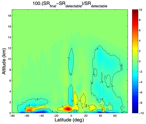
Figure 11Relative difference (in %) between the SR_observable field and the SR_detectable field both computed by E3SMv1, as a function of latitude and altitude.
Overall, the sampling bias introduced by the cloud-screening procedure does not significantly affect the mean SR values in E3SMv1. Therefore, errors in E3SMv1 clouds are not likely the primary reason for the differences in the aerosol seasonal comparison between E3SMv1 and CALIOP observations. In particular, the large difference observed at 60∘ S between the observed and simulated mean SR values cannot be explained by the large cloud screening in E3SMv1 at this latitude.
Nevertheless, cloud screening might have a larger impact on the mean aerosol CALIOP retrievals. Winker et al. (2013) found a lack of correlation between high semi-transparent cloud and aerosol in the lower troposphere in most regions in CALIOP data, implying that the screening of thin clouds does not significantly impact the retrieved values of aerosol optical depth or aerosol extinction coefficients. However, this result has to be extended to opaque cloud screening and has to be examined over a 3-month period at the specific locations that exhibit large cloud covers. To get an insight into the representativeness of our SR values retrieved from CALIOP, we computed the zonal-mean SR values over the MAM period by only considering one-third of the CALIOP data. We find that the relative difference between these SR values and those obtained by using the full CALIOP data is highest in covered regions, but it never exceeds 15 % (not shown). This gives us confidence about the robustness of our results retrieved by CALIOP over a 3-month period. An alternative approach would be to extend the analysis to cover multiple years, but the results would then be affected by the inter-annual variability of aerosol.
We can thus conclude that
-
the SR maxima retrieved by CALIOP over 3 months are robust and
-
the method of comparing modeled and retrieved SR is robust, although the modeled and observed clouds show large differences.
Therefore, the differences between observed and simulated SR values should be attributed to the representation of aerosol in the model.
Aerosol modeling basically consists of the representation of aerosol sources, optics, chemistry, micro-physics, aerosol–cloud interactions and transport. In the E3SMv1 model, aerosol optics is parameterized in terms of wet refractive index and wet surface mode radius of each mode (Ghan and Zaveri, 2007). It assumes volume mixing to compute the wet refractive index for mixtures of insoluble and soluble particles. The parameterization provides the aerosol extinction αa. We apply the same Ghan and Zaveri (2007) methodology and add the diagnostic variable of the 180∘ backscatter βa, as the aerosol lidar simulator requires these two input variables. Most GCMs compute the aerosol extinction, but not many of them routinely compute the aerosol 180∘ backscatter βa. Hence, more work has to be done so that other GCMs also diagnose their aerosol 180∘ backscatter βa in a way that is consistent with their aerosol optics parameterization. For future comparisons between CALIOP data and other GCMs, or for model-to-model comparisons, one might find it useful to use one single optics module to eliminate aerosol optics as a potential source of discrepancy in the comparisons. This is beyond the scope of this study and requires future investigation.
To evaluate the representation of aerosol composition in the model, the NASA product providing aerosol types from CALIPSO data is of particular interest. Indeed, CALIOP level 2 data include seven aerosol classes: clean marine, dust, polluted continental, clean continental, polluted dust, smoke and other. This classification utilizes the depolarization ratio, integrated attenuated backscatter coefficient, altitude, and land vs. ocean (Kim et al., 2018). The aerosol subtypes of CALIOP measurements have been shown to be in good agreement with the daily aerosol types derived from AERONET level 2.0 inversion data (Mielonen et al., 2009).
The CALIOP classification might be useful to provide insights into the model deficiency in representing aerosol composition in the model. According to this classification, the aerosol observed at 60∘ S during MAM is mostly clean marine aerosol. The large differences observed between CALIOP and E3SMv1 at this latitude may then be due to model biases in simulating marine aerosol in this region. Figure 9 in Rasch et al. (2019) and Fig. 11 in Wang et al. (2020) also show an aerosol bias over the Southern Ocean. There are certainly many possible reasons. The E3SMv1 model has both sea salt and marine organics as marine aerosol. Their “emissions” are function of surface winds and SST, based on Martensson et al. (2003). If the model has significant surface wind bias, that may thus impact the marine aerosol sources. Furthermore, McCoy et al. (2021) show that new particle formation (NPF) might be important in that region when they contrast SOCRATES field campaign measurements and Community Atmosphere Model version 6 (CAM6) simulations. This process is not well represented in the CAM6 model or in the E3SM model. We demonstrate here that the aerosol lidar simulator can be very useful in revealing these model biases, providing insights into future model development directions.
The validation of aerosol simulated by GCMs with space lidar data will be expanded to other lidars and to other GCMs. We plan to perform studies with the Laboratoire de Météorologie Dynamique Zoom (LMDZ) model, the European Center–Hamburg (ECHAM) model and the Icosahedral Nonhydrostatic (ICON) model. The modal aerosol module “HAM” that employs seven log-normal aerosol modes has been used interactively in the ECHAM model since almost two decades (Zhang et al., 2012; Tegen et al., 2019). Recently it is also implemented in the successor of ECHAM, the ICON model (Salzmann et al., 2022). The two models with profoundly different dynamical cores share the same physics package. It will be interesting to evaluate the differences induced by the two numerical representations of the atmospheric dynamics with the satellite retrievals.
Note that for a multi-model comparison, it is necessary to use a standard vertical grid with a coarser vertical resolution than N = 320 levels and Δz=60 m, as traditional climate models do not reach such a fine resolution. For the comparison of these models with CALIOP observations, data interpolation is needed on the same vertical coarser grid. Vertically averaging the CALIOP data would enhance the SNR and consequently would allow us to lower the aerosol detection threshold and make use of the more noisy CALIOP daily data. For each model it is important to check that the errors in the model clouds do not significantly impact the model–observation aerosol comparison over the considered period.
Since 2018, the Atmospheric Dynamics Mission Aeolus (ADM-Aeolus) has been operating the first high-spectral-resolution lidar (HSRL) in space. Although primarily dedicated to wind measurements, the HSRL capability in the UV allows the separation of the molecular and particulate contributions and enables the measurements of the particulate backscatter and extinction coefficients. These measurements provide new insight into very thin aerosol layers and can be very useful for the validation of models that directly compute these quantities. Later in 2023, the EarthCARE mission will also provide data from the HSRL lidar ATLID at 355 nm. The COSPv2 simulator can be easily adapted to other wavelengths, which opens the way to the determination of new diagnostics for cloud susceptibility, aerosol typing and aerosol–cloud proximity metrics.
The aerosol lidar simulator presented in this paper is available at https://doi.org/10.5281/zenodo.7418199 (Bonazzola and Chepfer, 2022) and is incorporated in the COSPv2 infrastructure at https://github.com/CFMIP/COSPv2.0 (last access: 9 December 2022).
The CALIPSO L1.5 data are available at https://doi.org/10.5067/CALIOP/CALIPSO/CAL_LID_L15-Standard-V1-01 (NASA/LARC/SD/ASDC, 2019). The processed gridded CALIOP ATB and SR data files used in this study are available at https://doi.org/10.5281/zenodo.7107232 (Bonazzola, 2022a) and https://doi.org/10.5281/zenodo.7107162 (Bonazzola, 2022b).
MB wrote the first version of this paper and conducted the analysis of this study; DMW, NS, JQ, and HC contributed to the design of the science objectives and the method of the study; PLM provided the GCM simulations and contributed to the code of the lidar aerosol module; AF gave technical support; and HC contributed to the code of the interface of the lidar aerosol simulator with the COSPv2 infrastructure. All authors contributed to the writing of the paper.
At least one of the (co-)authors is a member of the editorial board of Geoscientific Model Development. The peer-review process was guided by an independent editor, and the authors also have no other competing interests to declare.
Publisher's note: Copernicus Publications remains neutral with regard to jurisdictional claims in published maps and institutional affiliations.
We thank Rodrigo Guzman for his work on the development of the aerosol lidar simulator and on its interface with the COSPv2 infrastructure and Steve Klein for his inputs on the improvements of the vertical re-gridding within COSPv2. Po-Lun Ma was supported by the “Enabling Aerosol–cloud interactions at GLobal convection-permitting scalES (EAGLES)” project (no. 74358), funded by the U.S. Department of Energy (DOE), Office of Science, Office of Biological and Environmental Research, Earth System Model Development (ESMD) program area. The Pacific Northwest National Laboratory (PNNL) is operated for DOE by Battelle Memorial Institute under contract DE-AC05-76RL01830.
This research has been supported by the Centre National d'Etudes Spatiales (EECLAT) and the U.S. Department of Energy, Office of Science, Office of Biological and Environmental Research, Earth System Model Development (ESMD) program area (project no. 74358).
This paper was edited by Graham Mann and reviewed by Duncan Watson-Parris and one anonymous referee.
Bonazzola, M.: ATB CALIOP profiles, Zenodo [data set], https://doi.org/10.5281/zenodo.7107232, 2022a.
Bonazzola, M.: CALIOP SR profiles, Zenodo [data set], https://doi.org/10.5281/zenodo.7107162, 2022b.
Bonazzola, M. and Chepfer, H.: COSPv2.0: Adding lidar aerosol simulator, Zenodo [code], https://doi.org/10.5281/zenodo.7418199, 2022.
Cesana, G. and Chepfer, H.: How well do climate models simulate cloud vertical structure? a comparison between CALIPSO-GOCCP satellite observations and CMIP5 models, Geophys. Res. Lett., 39, L20803, https://doi.org/10.1029/2012GL053153, 2012.
Cesana, G. and Chepfer, H.: Evaluation of the cloud water phase in a climate model using CALIPSO-GOCCP, J. Geophys. Res., 118, 7922–7937, https://doi.org/10.1002/jgrd.50376, 2013.
Chepfer, H., Bony, S., Winker, D., Chiriaco, M., Dufresne, J.-L., and Sèze, G.: Use of CALIPSO lidar observations to evaluate the cloudiness simulated by a climate model, Geophys. Res. Lett., 35, L15704, https://doi.org/10.1029/2008GL034207, 2008.
Chepfer, H., Cesana, G., Winker, D., Getzewich, B., Vaughan, M., and Liu, Z.: Comparison of two different cloud climatologies derived from CALIOP-Attenuated Backscattered Measurements (Level 1): The CALIPSO-ST and the CALIPSO_GOCCP, J. Atmos. Ocean. Tech., 30, 725–744, https://doi.org/10.1175/JTECH-D-12-00057.1, 2013.
Chepfer, H., Noel, V., Chiriaco, M., Wielicki, B., Winker, D., Loeb, N., and Wood, R.: The Potential of a Multidecade Spaceborn Lidar Record to Constrain Cloud Feedback, J. Geophys. Res.-Atmos., 123, 5433–5454, 2018.
Costantino, L. and Bréon, F.-M.: Aerosol indirect effect on warm clouds over South-East Atlantic, from co-located MODIS and CALIPSO observations, Atmos. Chem. Phys., 13, 69–88, https://doi.org/10.5194/acp-13-69-2013, 2013.
Douville, H., Raghavan, K., Renwick, J., Allan, R. P., Arias, P. A., Barlow, M., Cerezo-Mota, R., Cherchi, A., Gan, T. Y., Gergis, J., Jiang, D., Khan, A., Pokam Mba, W., Rosenfeld, D., Tierney, J., and Zolina, O.: Water Cycle Changes, in: Climate Change: The Physical Science Basis. Contribution of Working Group I to the Sixth Assessment Report of the Intergovernmental Panel on Climate Change, edited by: Masson-Delmotte, V., Zhai, P., Pirani, A., Connors, S. L., Péan, C., Berger, S., Caud, N., Chen, Y., Goldfarb, L., Gomis, M. I., Huang, M., Leitzell, K., Lonnoy, E., Matthews, J. B. R., Maycock, T. K., Waterfield, T., Yelekçi, O., Yu, R., and Zhou, B., https://elib.dlr.de/137584/, 2021.
Forster, P., Storelvmo, T., Armour, K., Collins, W., Dufresne, J. -L., Frame, D., Lunt, D., Mauritsen, T., Palmer, M., Watanabe, M., Wild, M., and Zhang, H.: Chapter 7: The Earth’s energy budget, climate feedbacks, and climate sensitivity. Climate Change 2021: The Physical Science Basis. Contribution of Working Group I to the Sixth Assessment Report of the Intergovernmental Panel on Climate Change, edited by: Masson-Delmotte, V., Zhai, P., Pirani, A., Connors, S. L., Péan, C., Berger, S., Caud, N., Chen, Y., Goldfarb, L., Gomis, M. I., Huang, M., Leitzell, K., Lonnoy, E., Matthews, J. B. R., Maycock, T. K., Waterfield, T., Yelekçi, O., Yu, R., and Zhou, B., 2021.
Gelaro, R., McCarty, W., Suárez, M. J., Todling, R., Molod, A., Takacs, L., Randles, C. A., Darmenov, A., Bosilovich, M. G., Reichle, R., Wargan, K., Coy, L., Cullather, R., Draper, C., Akella, S., Buchard, V., Conaty, A., da Silva, A. M., Gu, W., Kim, G. K., Koster, R., Lucches, R., Merkova, D., Nielsen, J. E., Partyka, G., Pawson, S., Putman, W., Rienecker, M., Schubert, S. D., Sienkiewicz, M., and Zhao, B.: The modern-era retrospective analysis for research and applications, version 2 (MERRA-2), J. Climate, 30, 5419–5454, 2017.
Ghan, S. and Zaveri, R.: Parameterization of optical properties for hydrated internally mixed aerosol, J. Geophys. Re.-Atmos., 112, https://doi.org/10.1029/2006JD007927, 2007.
Golaz, J. C. , Caldwell, P., Van Roekel, L., Petersen, M., Tang, Q., Wolfe, J., Abeshu, G., Anantharaj, V., Asay-Davis, X., Bader, D., Baldwin, S., Bisht, G., Bogenschutz, P., Branstetter, M., Brunke, M., Brus, S., Burrows, S., Cameron-Smith, P., Donahue, A., Deakin, M., Easter, R., Evans,K., Feng, Y., Flanner, M., Foucar, J., Fyke, J., Griffin, B., Hannay, C., Harrop,B., Hoffman, M., Hunke, E., Jacob, R., Jacobsen, D., Jeffery, N., Jones, P., Keen, N., Klein, S., Larson, V., Leung, L. Li, H-Y., Lin, W., Lipscomb, W., Ma, P.-L., Mahajan, S., Maltrud, M., Mametjanov, A., McClean, J., McCoy, R., Neale, R., Price,S., Qian, Y., Rasch, P., Reeves, J., Eyre, J., Riley, W., Ringler, T., Roberts, A., Roesler, E., Salinger, A., Shaheen, Z., Shi, X., Singh, B., Tang, J., Taylor, M., Thornton, P., Turner, A., Veneziani, M., Wan, H., Wang, H-W.,Wang, S., Williams, D., Wolfram, P., Worley, P., Xie, S., Yang, Y., Yoon, J.-H., Zelinka, M., Zender, C., Zeng, X., Zhang, C., Zhang, K., Zhang, Y., Zheng, X., Zhou,T., and Zhu, Q.: The DOE E3SM Coupled Model Version 1: Overview and Evaluation at Standard Resolution, J. Adv. Model. Earth Sy., 11, 2089–2129, https://doi.org/10.1029/2018MS001603, 2019.
Guzman, R., Chepfer, H., Noel, V., Vaillant de Guelis, T., Kay, J. E., Raberanto, P., Cesana, G., Vaughan, M. A., and Winker, D. M.: Direct atmosphere opacity observations from CALIPSO provide new constraints on cloud-radiation interactions, J. Geophys. Res.-Atmos., 122, 1066–1085, https://doi.org/10.1002/2016JD025946, 2017.
Hodzic, A., Chepfer, H., Vautard, R., Chazette, P., Beekmann, M., Bessagnet, B., Drobinski, P., Goloub, P., Haeffelin, M., Morille, Y., Chatenet, B., and Cuesta, J.: Comparisons of aerosol chemistry-transport model simulations with lidar and sun-photometer observations at a site near Paris, J. Geophys. Res., 109, D23201, https://doi.org/10.1029/2004JD004735, 2004.
Hoesly, R. M., Smith, S. J., Feng, L., Klimont, Z., Janssens-Maenhout, G., Pitkanen, T., Seibert, J. J., Vu, L., Andres, R. J., Bolt, R. M., Bond, T. C., Dawidowski, L., Kholod, N., Kurokawa, J.-I., Li, M., Liu, L., Lu, Z., Moura, M. C. P., O'Rourke, P. R., and Zhang, Q.: Historical (1750–2014) anthropogenic emissions of reactive gases and aerosols from the Community Emissions Data System (CEDS), Geosci. Model Dev., 11, 369–408, https://doi.org/10.5194/gmd-11-369-2018, 2018.
Keating, T. and Zuber, A., Hemispheric transport of air pollution, Air Pollution Studies, 16, 2007.
Kim, M.-H., Lau, W., Kim, K.-M., and Lee, W.-S.: A GCM study of effects of radiative forcing of sulfate aerosol on large scale circulation and rainfall in East Asia during boreal spring, Geophys. Res. Lett., 34, https://doi.org/10.1029/2007GL031683, 2007.
Kim, M.-H., Omar, A. H., Tackett, J. L., Vaughan, M. A., Winker, D. M., Trepte, C. R., Hu, Y., Liu, Z., Poole, L. R., Pitts, M. C., Kar, J., and Magill, B. E.: The CALIPSO version 4 automated aerosol classification and lidar ratio selection algorithm, Atmos. Meas. Tech., 11, 6107–6135, https://doi.org/10.5194/amt-11-6107-2018, 2018.
Klein, S. A. and Jakob, C.: Validation and sensitivities of frontal clouds simulated by the ECMWF model, Mon. Weather Rev., 127, 2514–2531, 1999.
Koch, D. and Del Genio, A. D.: Black carbon semi-direct effects on cloud cover: review and synthesis, Atmos. Chem. Phys., 10, 7685–7696, https://doi.org/10.5194/acp-10-7685-2010, 2010.
Koffi, B., Schulz, M., Bréon, F. M., Griesfeller, J., Winker, D. M., Balkanski, Y., Bauer, S., Berntsen, T., Chin, M., Collins, W. D., Dentener, F., Diehl, T., Easter, R. C., Ghan, S. J., Ginoux, P. A., Gong, S., Horowitz, L. W., Iversen, T., Kirkevag, A., Koch, D. M., Krol, M., Myhre, G., Stier, P., and Takemura, T.: Application of the CALIOP layer product to evaluate the vertical distribution of aerosols estimated by global models: AeroCom phase I results, J. Geophys. Res., 117, D10201, https://doi.org/10.1029/2011JD016858, 2012.
Koffi, B., Schulz, M., Bréon, F. M., Dentener, F., Steensen, B. M., Griesfeller, J., Winker, D., Balkanski, Y., Bauer, S. E., Bellouin, N., Berntsen, T., Bian, H., Chin, M., Diehl, T., Easter, R., Ghan, S., Hauglustaine, D. A., Iversen, T., Kirkevåg, A., Liu, X., Lohmann, U., Myhre, G., Rasch, P., Seland, O., Skeie, R. B., Steenrod, S. D., Stier, P., Tackett, J., Takemura, T., Tsigaridis, K., Vuolo, M. R., Yoon, J., and Zhang, K.: Evaluation of the aerosol vertical distribution in global aerosol models through comparison against CALIOP measurements: AeroCom phase II results, J. Geophys. Res.-Atmos., 121, 7254–7283, https://doi.org/10.1002/2015JD024639, 2016.
Konsta, D., Dufresne, J. L., Chepfer, H., Idelkadi, A., and Cesana, G.: Use of A-train satellite observations (CALIPSO-PARASOL) to evaluate tropical cloud properties in the LMDZ5 GCM, Clim. Dynam., 47, 1263–1284, 2016.
Ma, P.-L., Rasch, P. J., Wang, M., Wang, H., Ghan, S., Easter, R. C., Gustafson, W., Liu, X., Zhang, Y., and Ma, H. Y.: How does increasing horizontal resolution in a global climate model improve the simulation of aerosol-cloud inteactions?, Geophys. Res. Lett., 42, 5058–5065, https://doi.org/10.1002/2015GL064183, 2015.
Ma, P. L., Rasch, P. J., Chepfer, H., Winker, D., and Ghan, S.: Observational constraint on cloud susceptibility weakened by aerosol retrieval limitations, Nat. Commun., 9, 2640, https://doi.org/10.1038/s41467-018-05028-4, 2018.
Ma, P.-L., Harrop, B. E., Larson, V. E., Neale, R. B., Gettelman, A., Morrison, H., Wang, H., Zhang, K., Klein, S. A., Zelinka, M. D., Zhang, Y., Qian, Y., Yoon, J.-H., Jones, C. R., Huang, M., Tai, S.-L., Singh, B., Bogenschutz, P. A., Zheng, X., Lin, W., Quaas, J., Chepfer, H., Brunke, M. A., Zeng, X., Mülmenstädt, J., Hagos, S., Zhang, Z., Song, H., Liu, X., Pritchard, M. S., Wan, H., Wang, J., Tang, Q., Caldwell, P. M., Fan, J., Berg, L. K., Fast, J. D., Taylor, M. A., Golaz, J.-C., Xie, S., Rasch, P. J., and Leung, L. R.: Better calibration of cloud parameterizations and subgrid effects increases the fidelity of the E3SM Atmosphere Model version 1, Geosci. Model Dev., 15, 2881–2916, https://doi.org/10.5194/gmd-15-2881-2022, 2022.
Martensson, E. M., Nilsson, E. D., De Leeuw, G., Cohen, L. H., and Hansson, H. C.: Laboratory simulations and parameterization of the primary marine aerosol production, J. Geophys. Res.-Atmos., 108, https://doi.org/10.1029/2002JD002263, 2003.
McCoy, I., Bretherton, C., Wood, R., Twohy, C., Gettelman, A., Bardeen, C., and Toohey, D.: Influences of Recent Particle Formation on Southern Ocean Aerosol Variability and Low Cloud Properties, J. Geophys. Res.-Atmos., 126, https://doi.org/10.1029/2020JD033529, 2021.
Mielonen, T., Arola, A., Komppula, M., Kukkonen, J., Koskinen, J., de Leeuw, K. G., and Lehtinen, E. J.: Comparison of CALIOP level 2 aerosol subtypes to aerosol types derived from AERONET inversion data, Geophys. Res. Lett., 36, https://doi.org/10.1029/2009GL039609, 2009.
NASA/LARC/SD/ASDC: CALIPSO Lidar Level 1.5 Profile, V1-01, NASA Langley Atmospheric Science Data Center DAAC [data set], https://doi.org/10.5067/CALIOP/CALIPSO/CAL_LID_L15-Standard-V1-01, 2019.
Quaas, J., Arola, A., Cairns, B., Christensen, M., Deneke, H., Ekman, A. M. L., Feingold, G., Fridlind, A., Gryspeerdt, E., Hasekamp, O., Li, Z., Lipponen, A., Ma, P.-L., Mülmenstädt, J., Nenes, A., Penner, J. E., Rosenfeld, D., Schrödner, R., Sinclair, K., Sourdeval, O., Stier, P., Tesche, M., van Diedenhoven, B., and Wendisch, M.: Constraining the Twomey effect from satellite observations: issues and perspectives, Atmos. Chem. Phys., 20, 15079–15099, https://doi.org/10.5194/acp-20-15079-2020, 2020.
Rasch, P., Xie, J. S., Ma, P. L., Lin, W., Wang, H., Tang, Q., Burrows, S. M., Caldwell, P., Zhang, K., Easter, R. C., Cameron-Smith, P., Singh, B., Wan, H., Golaz, J. C., Harrop, B. E., Roesler, E., Bacmeister, J., Larson, V. E., Evans, K. J., Qian, Y., Taylor, M., Leung, L. R., Zhang, Y., Brent, L., Branstetter, M., Hannay, C., Mahajan, S., Mametjanov, A., Neale, R., Richter, J. H., Yoon, J. H., Zender, C. S., Bader, D., Flanner, M., Foucar, J. G., Jacob, R., Keen, N., Klein, S. A., Liu, X. Salinger, A. G., Shrivastava, M., and Yang, Y.: An Overview of the Atmospheric Component of the Energy Exascale Earth System Model, J. Adv. Model. Earth Sy., 11, 2377–2411, 2019.
Ratnam, M. V., Prasad, P., Raj, S. T., Raman, M. R., and Basha, G.: Changing patterns in aerosol vertical distribution over South and East Asia, Sci. Rep., 11, 308, https://doi.org/10.1038/s41598-020-79361-4, 2021.
Reverdy, M., Chepfer, H., Donovan, D., Noel, V., Cesana, G., Hoareau, C., Chiriaco, M., and Bastin, S.: An EarthCARE/ATLID simulator to evaluate cloud description in climate models, J. Geophys. Res.-Atmos., 120, 11090–11113, https://doi.org/10.1002/2015JD023919, 2015.
Salzmann, M., Ferrachat, S., Tully, C., Münch, S., Watson-Parris, D., Neubauer, D., Siegenthaler-Le Drian, C., Rast, S., Heinold, B., Crueger, T., Brokopf, R., Mülmenstädt, J., Quaas, J., Wan, H., and Zhang, K.: The global atmosphere-aerosol model ICON-A-HAM2.3 – Initial model evaluation and effects of radiation balance tuning on aerosol optical thickness. J. Adv. Model. Earth Syst., 14, https://doi.org/10.1029/2021MS002699, 2022.
Stier, P.: Limitations of passive remote sensing to constrain global cloud condensation nuclei, Atmos. Chem. Phys., 16, 6595–6607, https://doi.org/10.5194/acp-16-6595-2016, 2016.
Stromatas, S., Turquety, S., Menut, L., Chepfer, H., Péré, J. C., Cesana, G., and Bessagnet, B.: Lidar signal simulation for the evaluation of aerosols in chemistry transport models, Geosci. Model Dev., 5, 1543–1564, https://doi.org/10.5194/gmd-5-1543-2012, 2012.
Swales, D., Pincus, R., and Bodas-Salcedo, A.: The Cloud Feedback Model Intercomparison Project Observational Simulator Package: Version 2 : Geosci. Model Dev., 11, 77-81, 2018
Szopa, S., Naik, V., Adhikary, B., Artaxo, P., Berntsen, T., Collins, W. D., Fuzzi, S., Gallardo, L., Kiendler Scharr, A., Klimont, Z., Liao, H., Unger, N., and Zanis, P.: Short-Lived Climate Forcers, in: Climate Change 2021: The Physical Science Basis. Contribution of Working Group I to the Sixth Assessment Report of the Intergovernmental Panel on Climate Change, edited by: Masson-Delmotte, V., Zhai, P., Pirani, A., Connors, S. L., Péan, C., Berger, S., Caud, N., Chen, Y., Goldfarb, L., Gomis, M. I., Huang, M., Leitzell, K., Lonnoy, E., Matthews, J. B. R., Maycock, T. K., Waterfield, T., Yelekçi, O., Yu, R., and Zhou, B., IPCC, 2021.
Tegen, I., Neubauer, D., Ferrachat, S., Siegenthaler-Le Drian, C., Bey, I., Schutgens, N., Stier, P., Watson-Parris, D., Stanelle, T., Schmidt, H., Rast, S., Kokkola, H., Schultz, M., Schroeder, S., Daskalakis, N., Barthel, S., Heinold, B., and Lohmann, U.: The global aerosol–climate model ECHAM6.3–HAM2.3 – Part 1: Aerosol evaluation, Geosci. Model Dev., 12, 1643–1677, https://doi.org/10.5194/gmd-12-1643-2019, 2019.
Tian, P., Cao, X., Zhang, L., Sun, N., Sun, L., Logan, T., Shi, J., Wang, Y., Ji, Y., Lin, Y., Huang, Z., Zhou, T., Shi, Y., and Zhang, R.: Aerosol vertical distribution and optical properties over China from long-term satellite and ground-based remote sensing, Atmos. Chem. Phys., 17, 2509–2523, https://doi.org/10.5194/acp-17-2509-2017, 2017.
van Marle, M. J. E., Kloster, S., Magi, B. I., Marlon, J. R., Daniau, A.-L., Field, R. D., Arneth, A., Forrest, M., Hantson, S., Kehrwald, N. M., Knorr, W., Lasslop, G., Li, F., Mangeon, S., Yue, C., Kaiser, J. W., and van der Werf, G. R.: Historic global biomass burning emissions for CMIP6 (BB4CMIP) based on merging satellite observations with proxies and fire models (1750–2015), Geosci. Model Dev., 10, 3329–3357, https://doi.org/10.5194/gmd-10-3329-2017, 2017.
Vuolo, M. R., Chepfer, H., Menut, L., and Cesana, G.: Comparison of mineral dust layers vertical structures modelled with Chimere-Dust and observed with the Caliop lidar, J. Geophys. Res., 114, https://doi.org/10.1029/2008JD011219, 2009.
Wang, Y., Yuan, Q., Shen, H., Zheng, L., and Zhang, L.: Investigating Multiple Aerosol Optical Depth products from MODIS and VIIRS over Asia: Evaluation, Comparison and Merging, Atmos. Environ., 230, https://doi.org/10.1016/j.atmosenv.2020.117548, 2020.
Waquet, F., Riedi, J., Labonnote, L. C., Goloub, P., Cairns, B., Deuzé, J.-L., and Tanré, D.: Aeorosol Remote Sensing over Clouds Using A-Train Observations, J. Atmos. Sci., 66, 2468–2480, 2009.
Watson-Parris, D., Schutgens, N., Winker, D., Burton, S. P., Ferrare, R. A., and Stier, P.: On the limits of CALIOP for constraining modeled, free tropospheric aerosol, Geophys. Res. Lett., 45, 9260–9266, https://doi.org/10.1029/2018GL078195, 2018.
Winker, D. M., Tackett, J. L., Getzewich, B. J., Liu, Z., Vaughan, M. A., and Rogers, R. R.: The global 3-D distribution of tropospheric aerosols as characterized by CALIOP, Atmos. Chem. Phys., 13, 3345–3361, https://doi.org/10.5194/acp-13-3345-2013, 2013.
Xie, S., Lin, W., Rasch, P., Ma, P.-L., Neale, R., Larson, V., Qian, Y., Bogenschutz, P., Caldwell, P., Smith, P., Golaz, J.-C., Mahajan, S., Singh, B., Tang, Q. I., Wang, H., Yoon, J.-H., Zhang, K., and Zhang, Y.: Understanding cloud and convective characteristics in version 1 of the E3SM atmosphere model, J. Adv. Model. Earth Sy., 10, 2618–2644, https://doi.org/10.1029/2018MS001350, 2018.
Yu, H., Chin, M., Winker, D. M., Omar, A. H., Liu, Z., Kittaka, C., and Diehl, T.: Global view of aerosol vertical distributions from CALIPSO lidar measurements and GOCART simulations: Regional and seasonal variations, J. Geophys. Res.-Atmos., 115, https://doi.org/10.1029/2009JD013364, 2010.
Zarzycki, M. and Bond, T. C.: How much can the vertical distribution of black carbon affect its global direct radiative forcing?, Geophys. Res. Lett., 37, L20807, https://doi.org/10.1029/2010GL044555, 2010.
Zhang, K., O'Donnell, D., Kazil, J., Stier, P., Kinne, S., Lohmann, U., Ferrachat, S., Croft, B., Quaas, J., Wan, H., Rast, S., and Feichter, J.: The global aerosol-climate model ECHAM-HAM, version 2: sensitivity to improvements in process representations, Atmos. Chem. Phys., 12, 8911–8949, https://doi.org/10.5194/acp-12-8911-2012, 2012.
Zhang, K., Wan, H., Liu, X., Ghan, S. J., Kooperman, G. J., Ma, P.-L., Rasch, P. J., Neubauer, D., and Lohmann, U.: Technical Note: On the use of nudging for aerosol–climate model intercomparison studies, Atmos. Chem. Phys., 14, 8631–8645, https://doi.org/10.5194/acp-14-8631-2014, 2014.