Multidecadal and climatological surface current simulations for the southwestern Indian Ocean at 1∕50° resolution

The Western INDian Ocean Simulation (WINDS) is a regional configuration of the Coastal and Regional Ocean Community Model (CROCO) for the southwestern Indian Ocean. WINDS has a horizontal resolution of $\mathrm{1}/\mathrm{50}$^∘ (∼2 km) and spans a latitudinal range of 23.5^∘ S–0^∘ N and a longitudinal range from the East African coast to 77.5^∘ E. We ran two experiments using the WINDS configuration: WINDS-M, a full 28-year multidecadal run (1993–2020); and WINDS-C, a 10-year climatological control run with monthly climatological forcing. WINDS was primarily run for buoyant Lagrangian particle tracking applications, and horizontal surface velocities are output at a temporal resolution of 30 min. Other surface fields are output daily, and the full 3D temperature, salinity, and velocity fields are output every 5 d. We demonstrate that WINDS successfully manages to reproduce surface temperature, salinity, currents, and tides in the southwestern Indian Ocean, and it is therefore appropriate for use in regional marine dispersal studies for buoyant particles or other applications using high-resolution surface ocean properties.

1 Introduction

The western Indian Ocean is a relatively data-sparse region. Surface current data are required to simulate the dispersion of buoyant particles such as marine debris or coral larvae (van Sebille et al., 2018), and whilst global products exist that cover the southwestern Indian Ocean, derived from satellite altimetry (e.g. Rio et al., 2014) and global ocean reanalyses (e.g. Lellouche et al., 2021), these products are at a coarse resolution relative to the scales of larval dispersal and do not resolve sub-mesoscale dynamics which are thought to be important for larval transport (e.g. Monismith et al., 2018; Dauhajre et al., 2019; Grimaldi et al., 2022). Some higher resolution models have been run in the southwestern Indian Ocean, but these simulations only spanned a limited subset of coral reefs within the region and are not available on publicly accessible repositories (Mayorga-Adame et al., 2016, 2017; Miramontes et al., 2019). Our objectives were to (1) provide improved estimates of regional surface currents across the tropical southwestern Indian Ocean, including at sub-mesoscale, and (2) estimate the connectivity (and temporal variability of connectivity) of coral reefs across the region, including the Chagos Archipelago. Bridging the gap between the fine-scale dynamics that dominate in coastal seas and large-scale ocean currents and mesoscale variability in the high seas is a major challenge in modelling larval dispersal (Edmunds et al., 2018). Future developments in unstructured ocean models, and improvements in the availability of computational resources, will be invaluable in addressing these challenges. However, for this study, we used a $\mathrm{1}/\mathrm{50}$^∘ (∼2 km) configuration of a regional (structured) ocean model to simulate circulation in the southwestern Indian Ocean, which we call the Western INDian Ocean Simulation (WINDS). Here, we provide a full description of WINDS and the two experiments we ran using the configuration, and we validate WINDS as relevant for buoyant Lagrangian particle tracking applications.

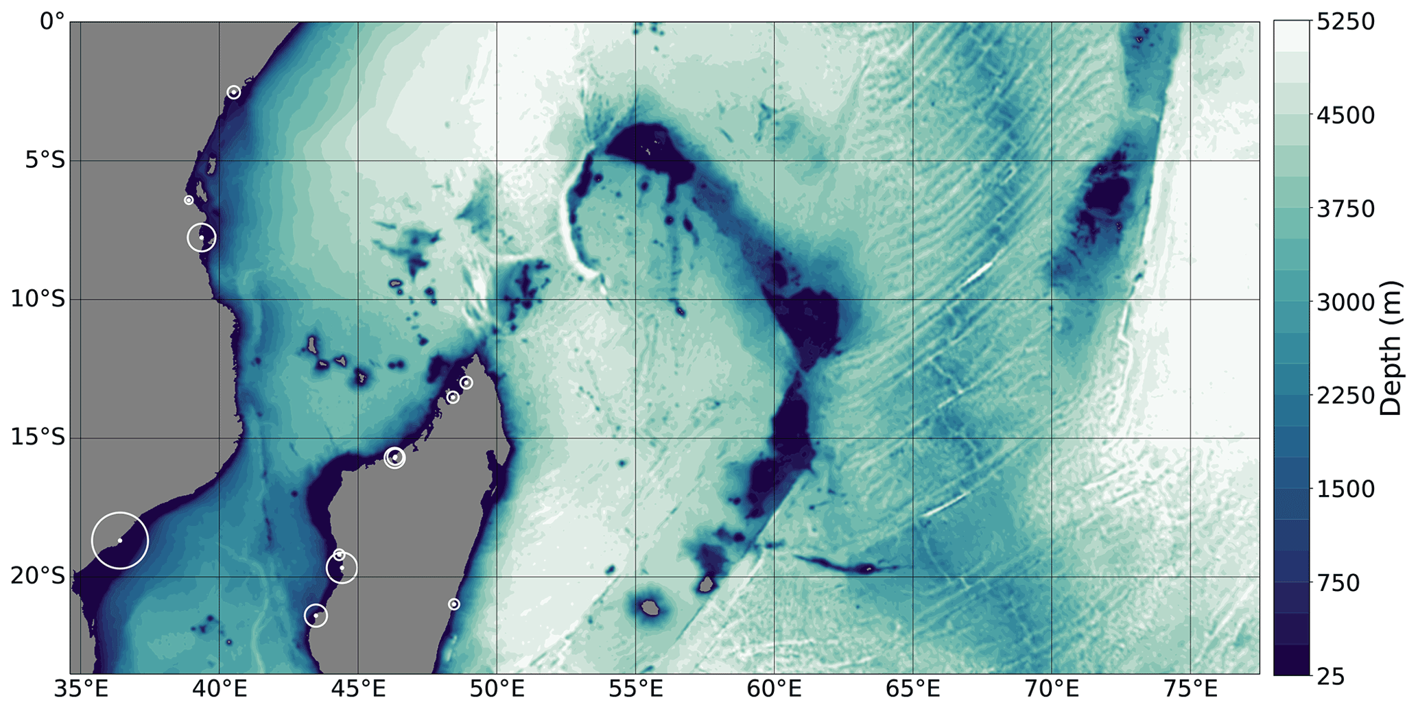
Figure 1 The entire WINDS domain, with contours representing the bathymetry used in WINDS. Circles represent the 12 rivers included in WINDS, scaled by the total annual discharge (Dai and Trenberth, 2002).

2 Methods

2.1 Numerics

We ran WINDS using version 1.1 of the Coastal and Regional Ocean Community Model (Auclair et al., 2019; Jullien et al., 2022) coupled with the XIOS2.5 I/O server for writing model output (https://forge.ipsl.jussieu.fr/ioserver, last access: 14 February 2023). WINDS uses a nonlinear equation of state (Jackett and Mcdougall, 1995; Shchepetkin and McWilliams, 2003) with a third-order upstream biased scheme for lateral momentum advection, a split-and-rotated third-order upstream biased scheme for lateral tracer advection, a fourth-order compact scheme for vertical momentum advection, and a fourth-order centred scheme with harmonic averaging for vertical tracer advection. Lateral momentum mixing is achieved through a Laplacian Smagorinsky parameterisation (Smagorinsky, 1963), and a generic length-scale k-ϵ scheme is used for vertical mixing (Jones and Launder, 1972). A bulk formulation is used for surface turbulent fluxes (COARE3p0) with current feedback enabled. The configuration uses radiative boundary conditions for forcing at the lateral boundaries (including non-tidal and tidal sea-surface height (SSH), barotropic tidal currents and baroclinic non-tidal currents, and temperature and salinity). A 10-point cosine-shaped sponge layer is also used at the lateral boundaries for tracers and momentum. Bottom friction is implemented using quadratic friction with a log-layer drag coefficient, with $z_{\mathrm{0},\mathrm{b}}=\mathrm{0.02}$ m and $\mathrm{0.002}\le C_{\mathrm{d}}\le \mathrm{0.1}$ (limits chosen for numerical stability). We used a baroclinic time step of 90 s, with 60 barotropic steps per baroclinic step (Shchepetkin and McWilliams, 2005).

2.2 Model grid

We built the model grid using CROCO_TOOLS with longitudinal limits 34.62^∘ S–77.5^∘ E, latitudinal limits of 23.5^∘ S–0^∘ N, and a specified horizontal resolution of $\mathrm{1}/\mathrm{50}$^∘ (Fig. 1). The western boundary of the domain is entirely land (East Africa). We chose this domain as it spans almost all coral reefs in the southwestern Indian Ocean and the Chagos Archipelago, allowing connectivity between the Chagos Archipelago and the rest of the southwestern Indian Ocean to be investigated. A small number of coral reefs southward of 23.5^∘ S (in southernmost Madagascar and South Africa) are therefore excluded, but this was necessary to keep computational and storage requirements tractable. To maintain roughly even dimensions of grid cells across the domain, CROCO_TOOLS adjusts the meridional resolution of cells away from the Equator, so the true meridional resolution of grid cells at the southern boundary of the WINDS domain is slightly finer, at around $\mathrm{1}/\mathrm{55}$^∘. The horizontal resolution of WINDS is therefore approximately 2 km but actually ranging from 2.04 km at the southern boundary to 2.22 km at the Equator.

CROCO uses a terrain-following (s coordinate) grid in the vertical. We used 50 vertical layers in WINDS, using a vertical stretching scheme that improves the resolution at the surface and bottom boundary layers, defined by the parameters θ_s=8, θ_b=2, and h_c=100 m (see the CROCO documentation for the technical explanation of these parameters). Since s coordinates are terrain (and sea-surface)-following, translating s coordinates to depth depends on the local ocean depth and the sea-surface height. The minimum and maximum ocean depth permitted in WINDS is 25 and 5250 m respectively. For water depth of 25 m and η=0 m, the vertical resolution is 0.40 m at the surface, 0.67 m at the sea floor, and the coarsest vertical resolution within the water column is 0.74 m. For water depth of 5250 m, the vertical resolution is 2.07 m at the surface, 280 m at the sea floor, and the coarsest vertical resolution within the water column is 353 m. As a result, WINDS provides excellent vertical resolution within the upper water column, particularly in shelf seas where coral reefs are.

2.3 Bathymetry

We use GEBCO 2019 (GEBCO Compilation Group, 2019) as the basis for the bathymetry in WINDS. The nominal horizontal resolution of GEBCO 2019 is 15 arcsec (approximately 500 m), but due to the lack of in situ bathymetry measurements in the southwestern Indian Ocean, most bathymetry in this region is satellite derived, with a practical resolution of around 6 km (Tozer et al., 2019). Although these satellite-derived measurements are relatively well validated, there are problems in areas of extensive continental shelves and steep bathymetry (Tozer et al., 2019). These problems are quite dramatic in the southwestern Indian Ocean. For instance, through comparison with Admiralty hydrographic navigation charts with in situ soundings, we found local bathymetry errors in excess of 1 km around Aldabra Atoll, Seychelles, and a large number of erroneous “islands” across Seychelles, which are in reality in significant water depth. Unfortunately, the only real solution to this lack of data is obtaining more in situ bathymetric readings (e.g. see Mayer et al., 2018). However, to somewhat mitigate the most extreme errors in the southwestern Indian Ocean, we carried out two preprocessing steps of the GEBCO 2019 dataset. We firstly digitised all point-depth soundings from Admiralty Chart 718 (Islands North of Madagascar), including Aldabra, Assomption, Cosmoledo, Astove, and the Glorioso islands, and then linearly gridded these data points onto a regular 15 arcsec grid, carrying out necessary tidal adjustments, before linearly blending these grids with the rest of the GEBCO 2019 grid across a length scale of 10–30 km. Secondly, to remove erroneous “islands”, we generated a land–sea mask at the GEBCO 2019 resolution from the highest resolution version of the GSHHG shoreline database (Wessel and Smith, 1996). We then set the depth of all false land cells (i.e. land according to GEBCO, ocean according to GSHHG) to 25 m. To avoid discontinuities in bathymetry, we applied a smooth tanh ramp between 25–50 m to all “true” ocean cells shallower than 50 m (i.e. the shallower the bathymetry above 50 m, the more strongly the bathymetry would be nudged towards 50 m, with all bathymetry shallower 25 m shifted to deeper than 25 m). Although this minimum depth of 25 m is not realistic, it is a considerable improvement over a large number of fake islands, and a minimum depth of around 25 m is required for numerical stability at this resolution by CROCO anyway. As a final processing step, we carried out smoothing of bathymetry using CROCO_TOOLS, with a target $\mathrm{\nabla }h/h=\mathrm{0.25}$ m⁻¹, to improve model stability and reduce pressure-gradient errors in regions of steep bathymetry. The bathymetry and associated grid parameters used in all WINDS simulations can be found in the croco_grd.nc file in the associated datasets, and the bathymetry is shown in Fig. 1.

2.4 Experiments: WINDS-C and WINDS-M

WINDS is forced at the surface through a bulk formulation based on ERA-5 (Hersbach et al., 2020) and at the lateral boundaries with the $\mathrm{1}/\mathrm{12}$^∘ GLORYS12V1 global ocean reanalysis (Lellouche et al., 2021) and tides. To investigate the importance of interannual variability in circulation in the southwestern Indian Ocean, we ran two experiments within WINDS. The first, WINDS-C, is based on a monthly climatology computed from ERA-5 and GLORYS12V1 from 1993–2018. The second, WINDS-M, is based on hourly forcing from ERA-5 and daily forcing from GLORYS12V1 from 1993–2019, plus an additional year (2020) based on the associated $\mathrm{1}/\mathrm{12}$^∘ global ocean analysis (the reanalysis product for 2020 was not available at this point). It is important that WINDS-M spans multiple decades, to fully incorporate the effects of multidecadal variability in surface circulation, and therefore dispersal (Thompson et al., 2018). WINDS-C was run after a 4-year spin-up, and WINDS-M was run from the end state of WINDS-C. WINDS-C and WINDS-M are otherwise identical.

2.5 Surface forcing

Surface forcing is parameterised using a bulk formulation based on the ERA-5 global atmosphere reanalysis (Hersbach et al., 2020) at hourly (WINDS-M) or monthly climatological (WINDS-C) temporal resolution, using the following fields, bilinearly interpolated to the WINDS grid:

• Surface air temperature (t2m)

• Sea-surface temperature (sst)

• Sea-level pressure (msl)

• 10 m wind speed (u10, v10)

• Surface wind stress (metss, mntss)

• Specific humidity (q)

• Relative humidity (r)

• Precipitation rate (mtpr)

• Shortwave radiation flux (msnswrf)

• Longwave radiation flux (msnlwrf)

• Downwelling longwave radiation flux (msdwlwrf)

Unit conversions are required for most of these quantities to put them into the form used by CROCO. Since ERA-5 is computed on a different (coarser) grid to WINDS, there is a land–sea mask mismatch between ERA-5 and WINDS. To avoid terrestrial values erroneously being applied to ocean cells in WINDS, we masked out land values from ERA-5 using the ERA-5 land–sea mask and carried out a nearest neighbour interpolation over the small number of coastal WINDS cells that are counted as land cells in ERA-5.

2.6 Lateral forcing

2.6.1 Ocean currents

WINDS is forced at the lateral boundaries with the $\mathrm{1}/\mathrm{12}$^∘ GLORYS12V1 global ocean reanalysis, using daily mean (WINDS-M) or monthly climatological (WINDS-C) depth-varying ocean current velocities, sea-surface height, temperature, and salinity. GLORYS12V1 was run using tides and, as a result, we do expect there to be aliased tidal signals remaining in the daily mean sea-surface height fields. However, we computed that the amplitude of the strongest aliased tidal signals (both SSH and currents) should be at least 20× smaller than the true tidal signals and frequency-shifted to a period of 10–30 d. As a result, we do not expect that any remnant tidal signals in GLORYS12V1 will have any significant effect on tides in WINDS.

2.6.2 Tides

WINDS is forced at the lateral boundaries with 10 tidal constituents (barotropic tidal currents and surface height) from the TPXO9-atlas (Egbert and Erofeeva, 2002): M₂, S₂, N₂, K₂, K₁, O₁, P₁, Q₁, Mf, and Mm.

2.7 Rivers

We have simplistically included 12 major rivers in WINDS: the Zambezi, Rufiji, Tsiribihina, Mangoky, Ikopa, Betsiboka, Tana, Mahavavy Nord, Sambirano, Manambolo, Mananjary, and Ruvu rivers. We assume that water in the river-mouth area has a constant temperature of 25 ^∘C and a salinity of 15 PSU, with monthly climatological discharge set according to Dai and Trenberth (2002). These riverine fluxes enter the ocean through the nearest ocean cell to the river mouth, set through inspection from satellite imagery (Google Earth). The location and annual mean discharge of these rivers is shown in Fig. 1.

3 Data records

We have made three sets of output available from WINDS (Vogt-Vincent and Johnson, 2022a, b):

• Output frequency of 30 min

  • –

    Zonal surface velocity (u_surf)

  • –

    Meridional surface velocity (v_surf)

• Output frequency of 1 d

  • –

    Sea-surface temperature (temp_surf)

  • –

    Sea-surface salinity (salt_surf)

  • –

    Free-surface height (zeta)

  • –

    Depth-averaged zonal velocity (u_bar)

  • –

    Depth-averaged meridional velocity (v_bar)

  • –

    Kinematic wind stress (wstr)

  • –

    Surface zonal momentum stress (sustr)

  • –

    Surface meridional momentum stress (svstr)

  • –

    Surface freshwater flux, E-P (swflx)

  • –

    Surface net heat flux (shflx)

  • –

    Net shortwave radiation at surface (radsw)

  • –

    Net longwave radiation at surface (shflx_rlw)

  • –

    Latent heat flux at surface (shflx_lat)

  • –

    Sensible heat flux at surface (shflx_sen)

• Output frequency of 5 d

  • –

    Zonal velocity (u)

  • –

    Meridional velocity (v)

  • –

    Temperature (temp)

  • –

    Salinity (salt)

We did not output the vertical velocity. This can in principle be reconstructed at a 5 d frequency using the ocean depth, free-surface height, and zonal and meridional velocities.

4 Technical validation

The following validation relates to WINDS surface properties only, as relevant for marine dispersal, since this was the primary use case WINDS-M and WINDS-C were run for. WINDS may, of course, be used for other purposes as well, but for these applications the model is provided as is. This validation focuses on WINDS-M, since WINDS-C is a control simulation which is not expected to fully reproduce observations, as it is driven by low-frequency (monthly) climatological forcing.

4.1 Tides

We extracted the five largest tidal constituents (M₂, S₂, N₂, K₁, and O₁) at 50 sites across the WINDS domain (41 coastal and 9 open ocean) based on a 55 d 2-hourly time series from WINDS-M 1994, and we compared these amplitudes to the corresponding amplitudes in TPXO9-atlas (Egbert and Erofeeva, 2002) (see Table S1). Note that this comparison is not independent, since the TPXO9-atlas is used to set tidal boundary conditions at the WINDS domain boundaries. Additionally, TPXO9-atlas is not a purely observational product: it is a $\mathrm{1}/\mathrm{30}$^∘ inverse model constrained by observations. However, TPXO9-atlas is extensively validated, and good agreement between tides in WINDS and TPXO9 does at least suggest that WINDS is propagating TPXO9-atlas tides reasonably.

Agreement between WINDS and TPXO9 is generally good, with tidal amplitude mismatch on the order of a few centimetres for almost all sites (well within the error associated with the TPXO9-atlas itself). A few regions associated with greater WINDS-TPXO9 disagreement include (1) the Sofala Bank (Mozambique) and (2) the mainland-facing sides of Mafia and Zanzibar islands (Tanzania). Both are shelf regions with extensive shallow water and, in the case of Tanzania, complex effects from nearby islands. The roughness length scale used in the bottom friction parameterisation in WINDS is constant, and the true ocean depth at these locations is occasionally shallower than the minimum depth used in WINDS, so it is possible that a combination of these two factors could explain the poorer tidal performance of WINDS in some shelf seas.

We have also carried out a comparison of WINDS tidal predictions with selected in situ tidal gauges spanning the longitudinal and latitudinal range of WINDS, at Mombasa (Kenya), Aldabra (Outer Islands, Seychelles), Mahé (Inner Islands, Seychelles), Diego Garcia (Chagos Archipelago), and Mauritius and Rodrigues (Mauritius) (Table 1). This comparison demonstrates that WINDS can reproduce in situ tidal predictions well, particularly at remote islands away from extensive continental shelves.

Table 1 Observational sources: Pugh (1979) (Mombasa, Aldabra, and Mahé); Lowry et al. (2008) (Rodrigues and Mauritius); Dunne (2021) (Diego Garcia).

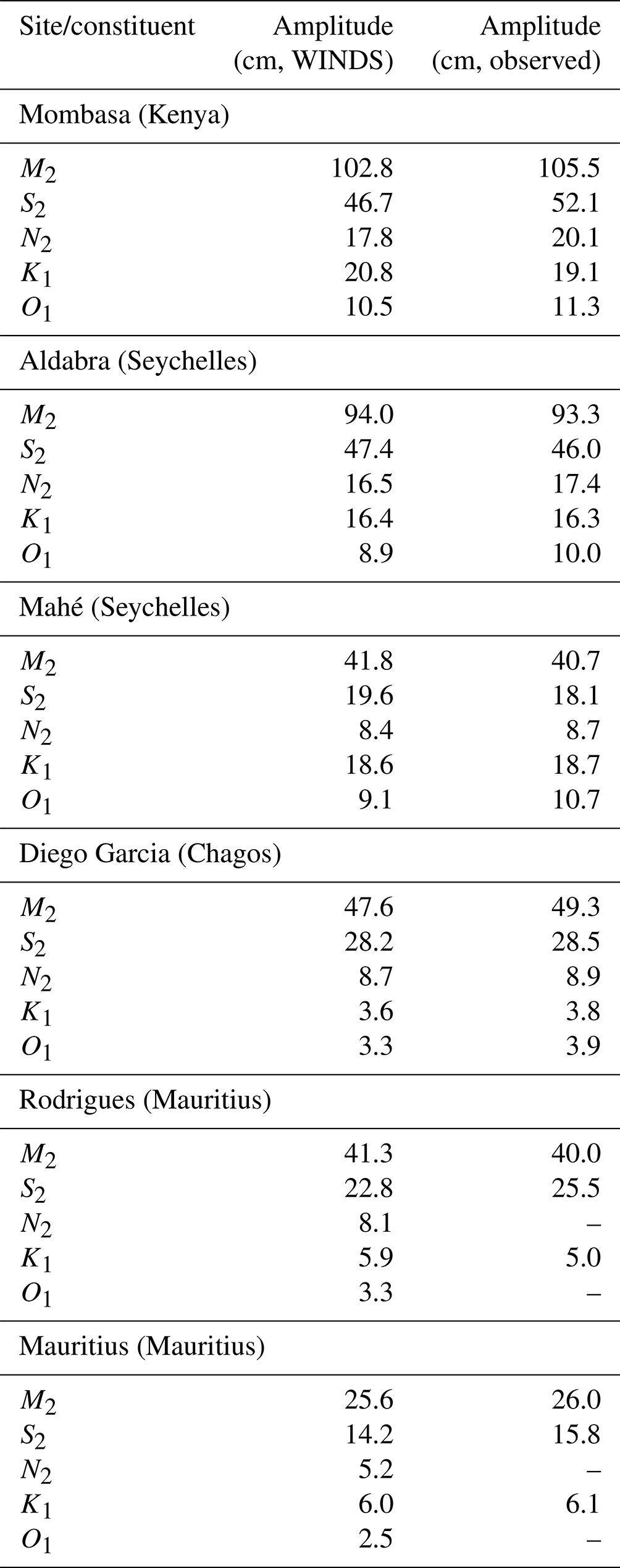
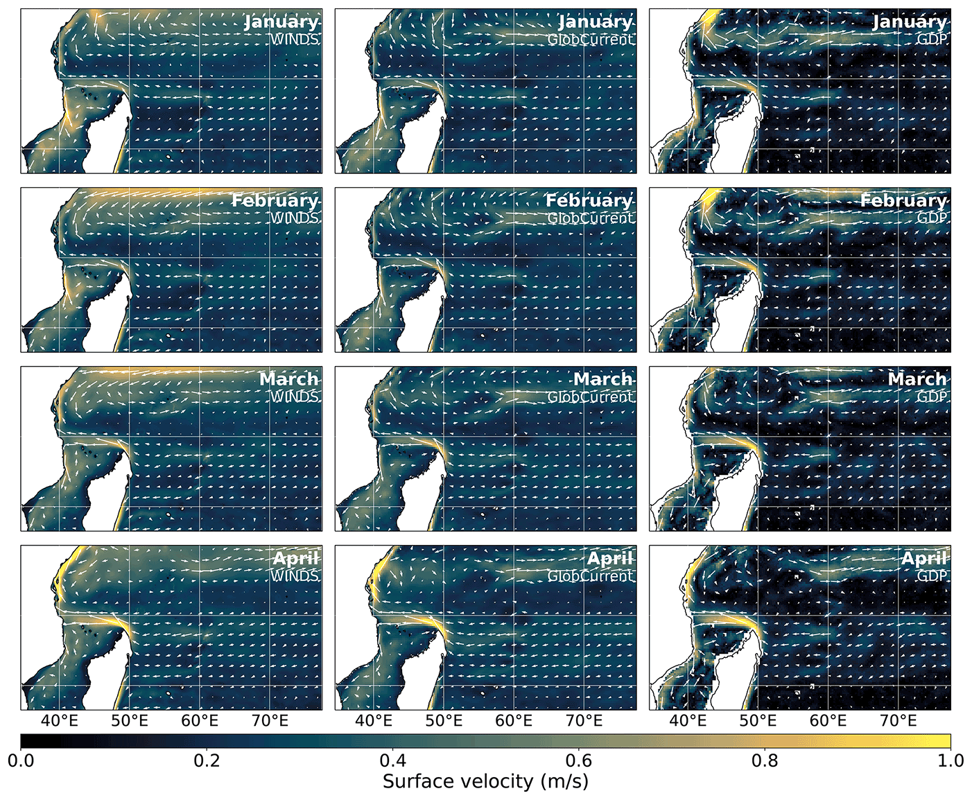
Figure 2 Monthly climatological surface currents (1993–2020) from WINDS (left), Copernicus GlobCurrent Surface (centre), and Global Drifter Program-derived near-surface currents (right) for January to April.

Figure 3 Monthly climatological surface currents (1993–2020) from WINDS (left), Copernicus GlobCurrent Surface (centre), and Global Drifter Program-derived near-surface currents (right) for May to August.

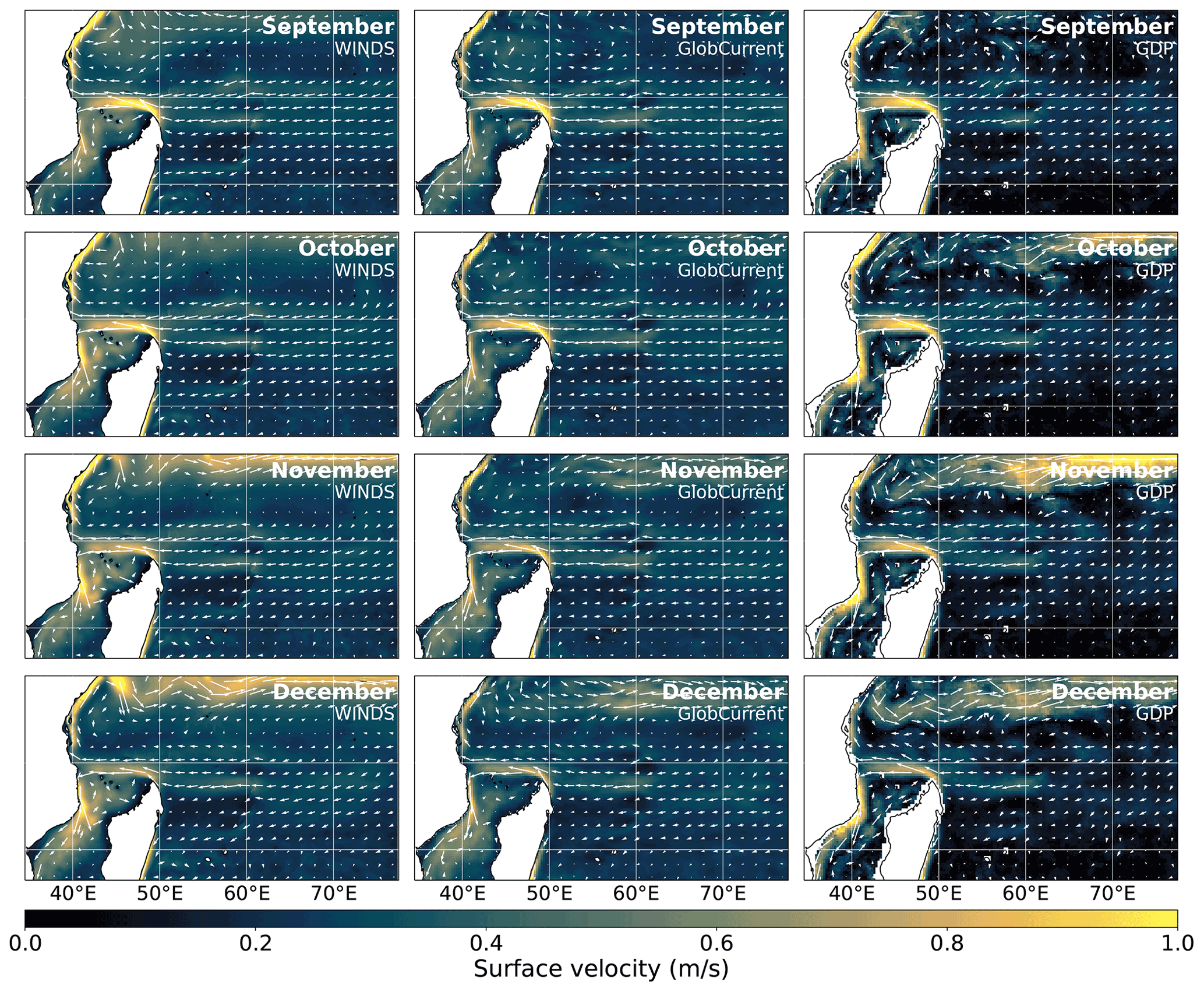
Figure 4 Monthly climatological surface currents (1993–2020) from WINDS (left), Copernicus GlobCurrent Surface (centre), and Global Drifter Program-derived near-surface currents (right) for September to December.

4.2 Surface currents

Figures 2–4 compare monthly climatological surface currents averaged across 1993–2020 from WINDS-M (left); surface currents from 1993–2020 from Copernicus GlobCurrent, combining altimetric geostrophic currents with modelled Ekman currents (centre, Rio et al., 2014); and near-surface currents estimated from the Global Drifter Program (GDP) using drifter trajectories from 1979–2015 (right, Laurindo et al., 2017). Both products used for comparison are entirely independent of WINDS. These figures demonstrate that WINDS successfully captures the location and velocity associated with major ocean currents in the southwestern Indian Ocean such as the Southern Equatorial Current, Southern Equatorial Countercurrent, North Madagascar Current, East Madagascar Current, and East African Coastal Current (e.g. Schott et al., 2009), as well as their seasonal variability. For instance, WINDS reproduces the observed strengthening of surface currents associated with the North Madagascar Current during the southeast monsoon (June–August), which can instantaneously reach 2 m s⁻¹, in accordance with in situ observations (Swallow et al., 1988; Voldsund et al., 2017). The East African Coast Current (EACC) also correctly strengthens dramatically during the southeast monsoon, also reaching speeds of up to (and sometimes exceeding) 2 m s⁻¹, in agreement with observations (Swallow et al., 1991; Painter, 2020). The strongest surface currents in the EACC are simulated by WINDS to be close to the Equator and can instantaneously reach 3 m s⁻¹. We are not aware of observational evidence supporting such strong surface currents within the EACC. There is a discrepancy between the strength of surface currents simulated by WINDS and predicted by GlobCurrent for the South Equatorial Countercurrent close to the Equator (e.g. see Fig. 4, November). However, this is unsurprising as GlobCurrent uses geostrophic currents, which are not defined at the Equator. Agreement between WINDS and GDP-derived surface velocities are much better in this region, with WINDS reproducing observations of zonal surface currents in excess of 1 m s⁻¹, particularly towards the east of the WINDS domain (Schott and McCreary, 2001; Shao-Jun et al., 2012).

To assess the ability of WINDS to reproduce surface current variability associated with eddies, Fig. 5 compares the eddy kinetic energy (EKE) in WINDS and Copernicus GlobCurrent (high-frequency surface currents are not available from the Global Drifter Program), as well as eight moorings from the RAMA array (McPhaden et al., 2009; Beal et al., 2019). The spatial pattern in EKE is similar between WINDS and Copernicus GlobCurrent, with both products returning high EKE associated with mesoscale eddy activity in the Mozambique Channel, around Mauritius and Réunion, in the wake of the Mascarene Plateau, and near the Equator. EKE is generally higher in WINDS than Copernicus GlobCurrent, although this is likely in part due to sub-mesoscale turbulence simulated by WINDS, which will not be captured by Copernicus GlobCurrent. Compared to in situ observations at RAMA array moorings, WINDS and Copernicus GlobCurrent tend to respectively overestimate and underestimate EKE. The RAMA time series is considerably shorter than WINDS-M, and most moorings do not record equal coverage across the seasonal cycle. However, there does not appear to be a strong seasonal cycle in EKE in most regions (Figs. S1–S3), so it is unlikely that this explains the systematically higher EKE in WINDS compared to RAMA. The currents measured at RAMA are also measured at a slightly greater depth (10/12 m) than WINDS (0–2 m). Nevertheless, this does suggest that eddies may be too energetic in WINDS. On the other hand, the variability of daily sea-surface height (Fig. 6), and therefore geostrophic surface currents, agrees very well with observations. This suggests that, at least away from the Equator, mesoscale eddy activity is reasonably reproduced in WINDS.

Figure 5 Eddy kinetic energy (EKE) from WINDS (top) and Copernicus GlobCurrent (bottom). EKE was computed by passing daily mean surface velocity through a high-pass filter with a cutoff period of 30 d, thereby removing high-frequency variability associated with tides, and low-frequency variability associated with time mean currents and the seasonal cycle. Circles represent the EKE at 10/12 m depth from the RAMA array. EKE is also plotted as a monthly climatology in Figs. S1–S3 and MKE (annual mean and monthly climatological) in Figs. S4–S7.

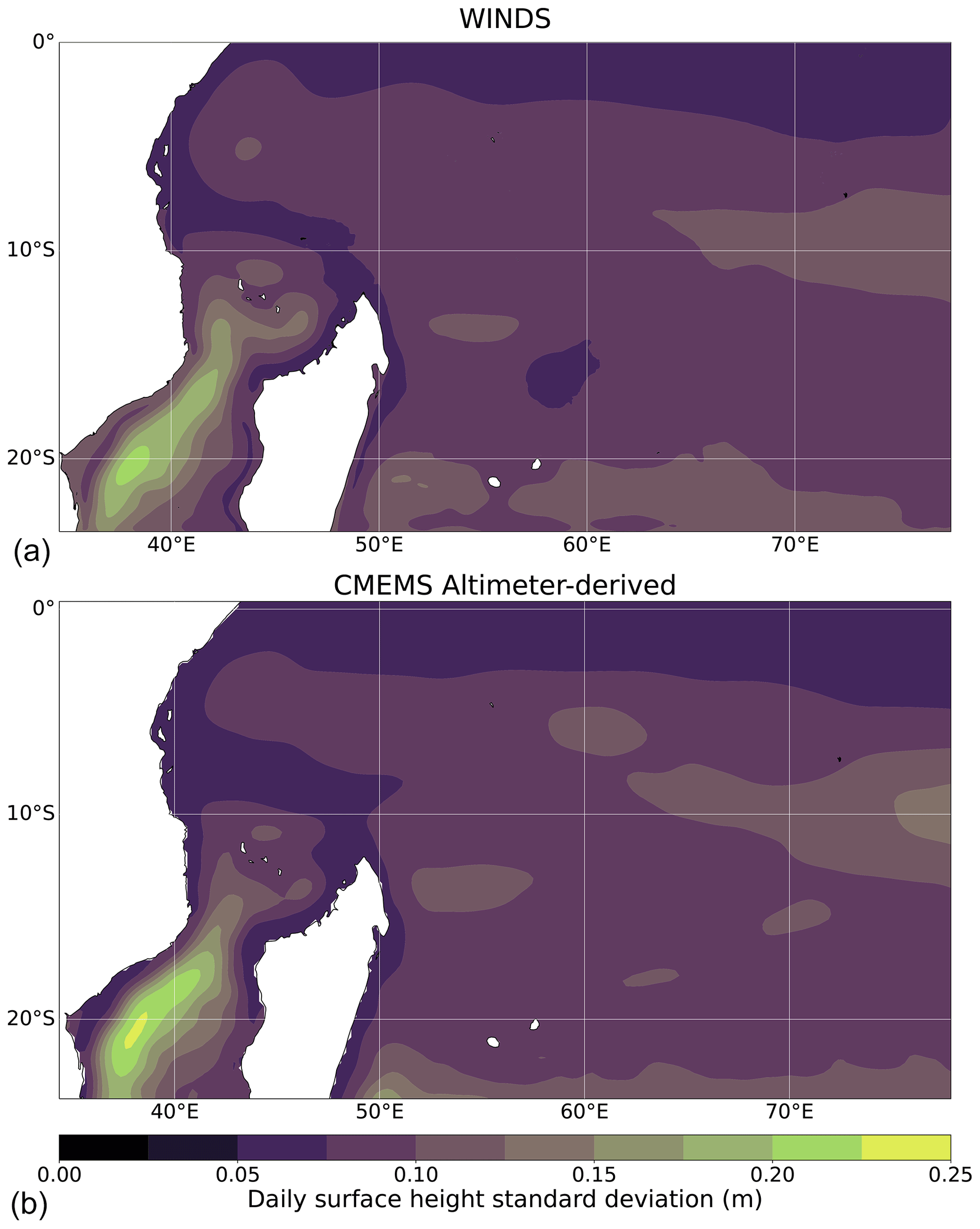
Figure 6 Variability of sea-surface height from 1993–2020 from WINDS (a) and the Copernicus Marine Environment Monitoring Service (CMEMS) Global Ocean Reprocessed Gridded L4 Sea Surface Height product (b), computed as a standard deviation.

Figure 7 Monthly mean surface currents averaged across 10 key regions (see Fig. S8 for geographical reference) for WINDS (black, with grey shading representing the monthly range), CMEMS GLORYS12V1 (red), and GlobCurrent (blue).

The monthly mean surface current speed in WINDS associated with major surface currents in the southwestern Indian Ocean is shown is Fig. 7 (see Fig. S8 for geographical reference), compared to a $\mathrm{1}/\mathrm{12}$^∘ global ocean reanalysis (Copernicus Marine Environment Monitoring Service – CMEMS – GLORYS12V1) and Copernicus GlobCurrent. Particularly strong agreement between GLORYS12V1 and GlobCurrent is expected, as the former is an assimilative model, but agreement is generally very good between all three products. One notable exception is the western South Equatorial Countercurrent, where current variability often appears to be greater in WINDS than GLORYS12V1 and GlobCurrent (which is also reflected in EKE derived from RAMA moorings in Fig. 5). The seasonal cycle is also amplified in the NW Mozambique Channel in WINDS compared to GLORYS12V1 and GlobCurrent. Very high surface current speeds have been observed in this region from in situ observations (Ridderinkhof et al., 2010), but it is not clear whether the stronger seasonality simulated by WINDS is real or an artefact. Although the seasonal monsoonal cycle dominates many of the time series in Fig. 7, it is also clear that there is considerable interannual variability. This is generally reproduced very well by WINDS, but the magnitude of interannual variability is occasionally larger in WINDS than GLORYS12V1 or GlobCurrent (see also Fig. S9).

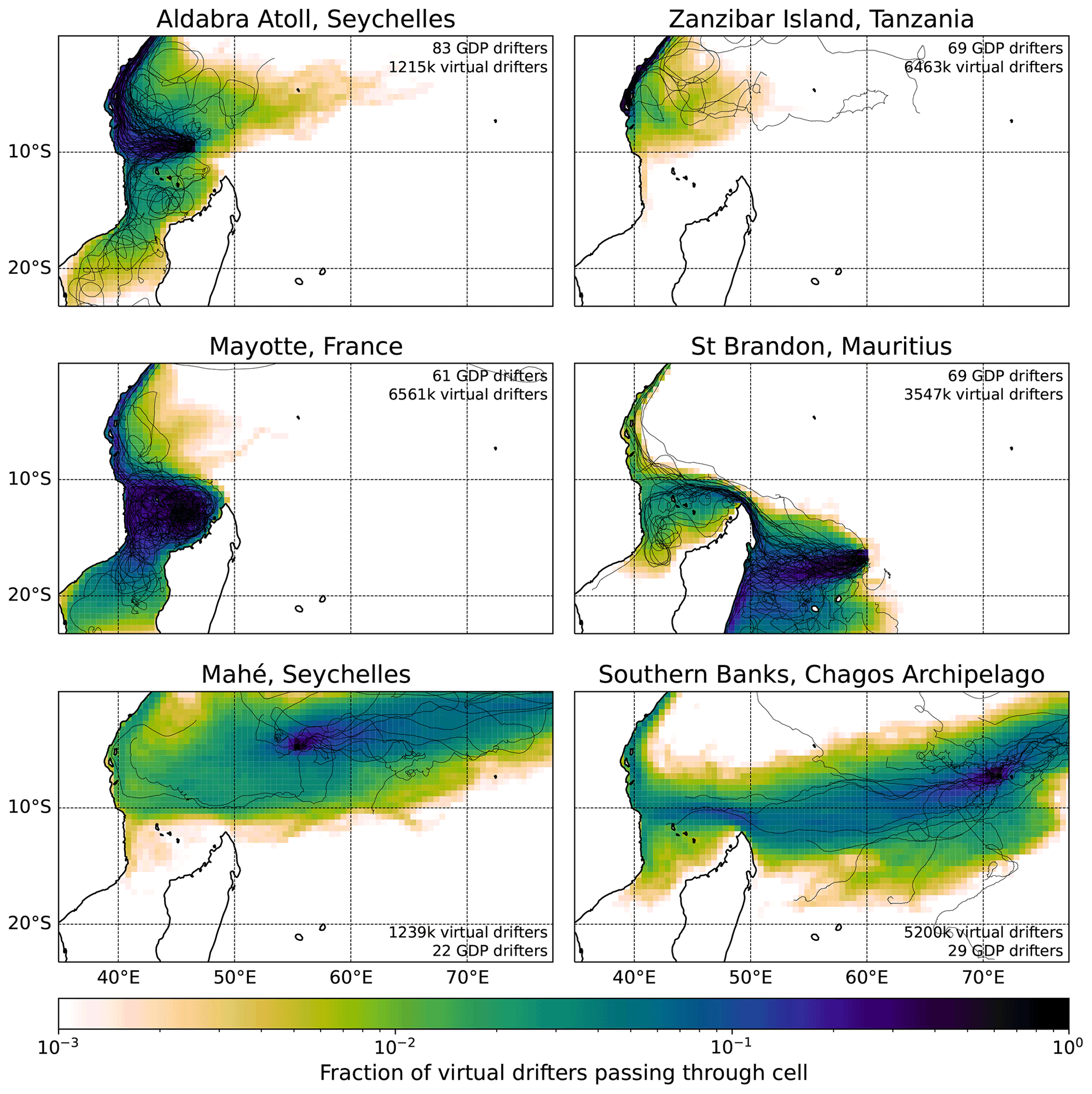
Figure 8 Colour: fraction of virtual drifters advected with half-hourly WINDS-M surface currents that pass through each 0.5^∘ × 0.5^∘ grid cell at least once within 120 d. Cells with less than 0.1 % of virtual drifters passing through are shaded in white. Lines: observed Global Drifter Program drifter trajectories for 120 d following the nearest pass to the virtual drifter release site (or until beaching/death if this occurred within 120 d).

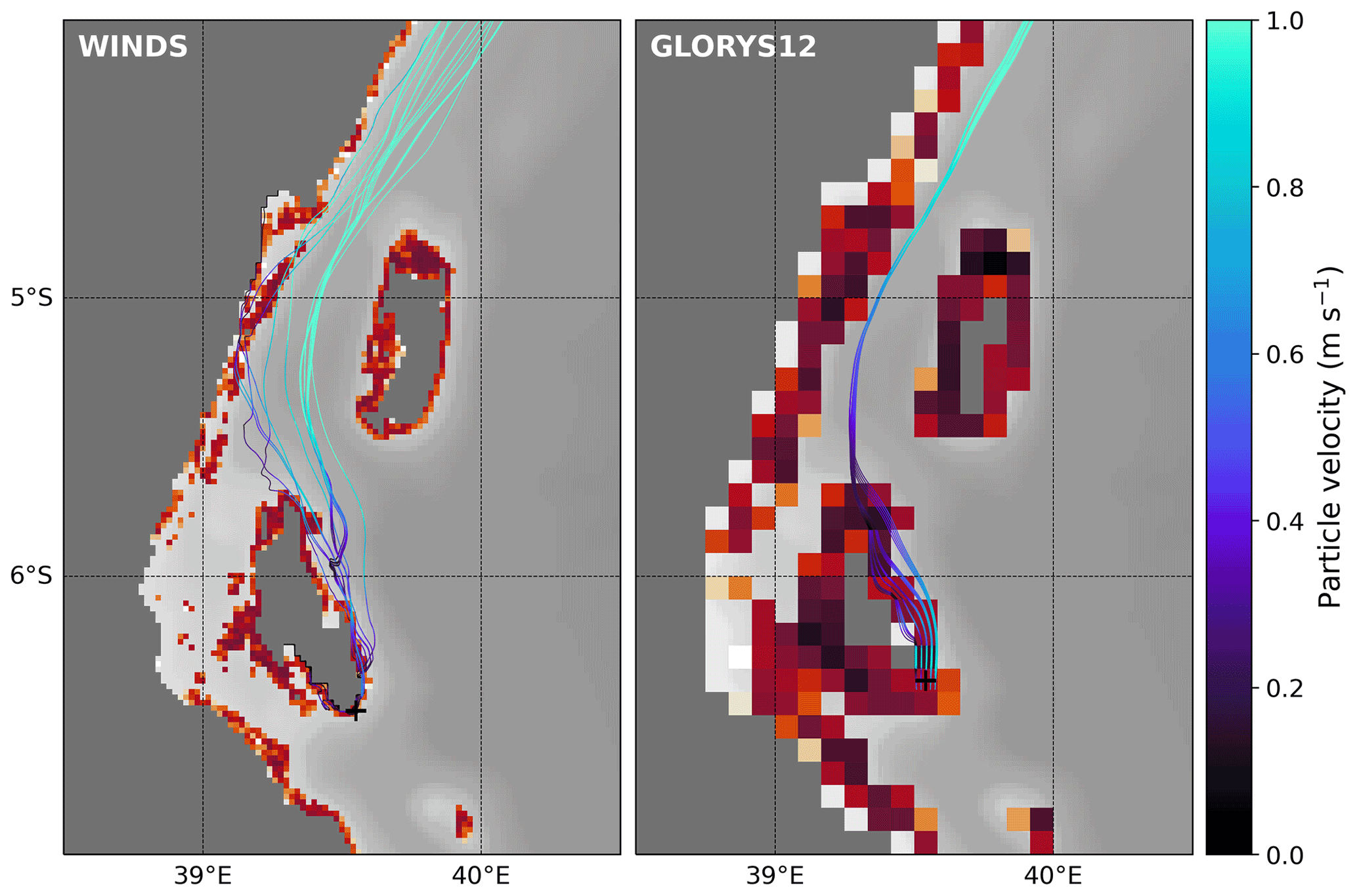
Figure 9 Coloured by instantaneous speed, 25 virtual drifter trajectories released from analogous coral reef cells at the southern tip of Zanzibar (Tanzania) on 1 July 2019 in WINDS-M (left) and GLORYS12V1 (right). Land cells for both models are shaded in dark grey. Red cells are coral reefs (Li et al., 2020), aggregated to the respective model grid, and shaded by total area per cell (shown for illustrative purposes only).

As WINDS was designed for the primary purpose of simulating marine dispersal (for instance, for coral larvae), it is important to test whether WINDS can reproduce observed pathways of surface drift in the ocean. Although Global Drifter Program (GDP) deployments are low in the southwestern Indian Ocean (Lumpkin and Centurioni, 2019), sufficient drifters have passed through the region to evaluate first-order dispersal pathways simulated by WINDS. We released a large number of virtual Lagrangian particles at coral reef sites around six islands and banks within the WINDS domain on the 1st, 11th, and 21st of each month from 1993–2019, and we advected them for 120 d following WINDS-M surface currents using OceanParcels (Lange and Sebille, 2017), with a Runge–Kutta fourth-order scheme and a time step of 10 min. Figure 8 shows the proportion of these virtual particles that passed through each 0.5^∘ × 0.5^∘ grid cell at least once within 120 d, overlaid with GDP drifter trajectories for (up to) 120 d after their nearest approach to release sites. Although the Global Drifter Program sample size is small in some cases, agreement between observed drifter trajectories and WINDS is generally excellent, with observed trajectories usually confined to the “high probability” regions predicted by WINDS. Notable exceptions include some GDP drifters that travelled further eastward within the South Equatorial Countercurrent from Mayotte and Zanzibar than predicted by WINDS and less zonal confinement within the South Equatorial Current for GDP drifters travelling westwards from the Chagos Archipelago as compared to WINDS. These trajectories are physically possible within WINDS (Fig. S10), but improbable. Surface currents associated with the South Equatorial Countercurrent in WINDS are generally at least as strong as those diagnosed from GDP drifters (Figs. 2–4), so the possible underprediction of eastward surface transport is instead likely due to the WINDS domain ending at the Equator. In our Lagrangian analysis, any virtual particles crossing the Equator are removed, so many virtual particles may be unable to enter the South Equatorial Countercurrent. For instance, most GDP drifters in Fig. 8 that travelled a significant distance within the South Equatorial Countercurrent passed the Equator at least once. It is nevertheless possible that WINDS underestimates surface connectivity between the East Africa Coastal Current and the South Equatorial Countercurrent, as one GDP drifter followed a relatively direct pathway from Zanzibar to the Seychelles Plateau, which was improbable in WINDS. It is important to note that GDP drifters are drogued and have some wind exposure due to the buoy, and may therefore experience forces from winds, waves, and subsurface currents which will not be captured by WINDS.

Figure 10 Difference between monthly climatological SST simulated by WINDS and satellite and in situ-derived sea-surface temperature (SST) estimates from the Operational Sea Surface Temperature and Sea Ice Analysis (OSTIA). Blues indicate that WINDS simulates cooler temperatures and reds indicate that WINDS is warmer.

Long-distance dispersal patterns predicted by WINDS are similar to those predicted by the CMEMS GLORYS12V1 $\mathrm{1}/\mathrm{12}$^∘ global ocean reanalysis (Fig. S11) and, given the relatively small sample size of GDP drifters in the region, it is not clear which product performs better over these very large distances. Indeed, this is expected, as the $\mathrm{1}/\mathrm{12}$^∘ horizontal resolution of GLORYS12V1 is likely sufficient to resolve the main processes relevant to the large-scale surface circulation in the Indian Ocean. The real potential advantage of WINDS is at finer scales, which is particularly important for local applications or for modelling the dispersal of substances with a lifespan on the order of days to weeks (rather than months or longer), such as coral larvae Connolly and Baird (2010). For instance, Fig. 9 shows simulated trajectories of 25 virtual surface-confined particles, perhaps representing coral larvae, released from analogous reef sites in southern Zanzibar, Tanzania, in WINDS-M and GLORYS12V1, at the same time on 1 July 2019. Perfect agreement between the two is not expected, as (i) WINDS is not assimilative and (ii) there was likely limited observational data available for assimilation in this region in the first place. However, it is clear from this figure that the representation of the coast and islands is significantly improved in WINDS relative to GLORYS12V1 (due to the more than 4-fold increase in horizontal resolution). For instance, some virtual particles in WINDS entered Kiwani Bay in southwestern Zanzibar, rather than entering the East Africa Coastal Current. This is physically impossible in GLORYS12V1, as the resolution is too coarse to resolve all but the largest coastal features. WINDS also simulates greater particle–particle dispersion due to resolved motion that would be subgrid scale for GLORYS12V1 (Poje et al., 2010). The approximately 2 km resolution of WINDS is still too coarse to resolve the finest scales of motion that are important for reef-scale dispersal (Dauhajre et al., 2019; Grimaldi et al., 2022), but at intermediate scales of tens to hundreds of kilometres, we expect that WINDS will provide a significantly improved capacity for dispersal modelling and associated applications as compared to existing openly available regional and global ocean simulations.

4.3 Sea-surface temperature (SST) and salinity (SSS)

We have validated WINDS SST and SSS predictions by comparing monthly climatological SST and SSS from WINDS-M to monthly climatological SST from OSTIA (Good et al., 2020) and SSS from ARMOR3D (Guinehut et al., 2012), all computed across 1993–2020 (both are independent of WINDS, although it is important to note that observations for sea-surface salinity are sparse in the southwestern Indian Ocean). In general, WINDS performs well for both SST and SSS; the mean absolute error (MAE) for SST and SSS respectively ranges between 0.14–0.24 ^∘C and 0.06–0.1 PSU across the seasonal cycle (Figs. 10 and S12). There is a widespread and year-round cold and fresh bias across most of the southwestern Indian Ocean in WINDS, although the magnitude of this bias is small. There is also a warm bias within the Mozambique Channel during the northwest monsoon (November to February) and a salty bias year round. We do not know for certain why these biases exist in WINDS, although it may be related to the GLS vertical mixing parameterisation, resulting in an over/underestimate of the mixed-layer depth. WINDS also appears to slightly overestimate the strength of the seasonal SST cycle in shallow water along the coasts of East Africa and Madagascar. Finally, there is a spatially limited but relatively intense fresh bias in WINDS off the coast of Mozambique, associated with the Zambezi River. The implementation of rivers in WINDS is simplistic, so it is possible that the seasonal discharge climatology or physical water properties associated with the river mouth (15 PSU and 25 ^∘C) were inappropriate, that the advection of the freshwater plume associated with the river is incorrectly simulated in WINDS, or that ARMOR3D does not fully capture the fine-scale freshwater plume associated with the Zambezi River. Figure S13 shows time series of the difference in SST and SSS between WINDS, and OSTIA and ARMOR3D, across the simulation time span. Errors in both SST and SSS follow a seasonal cycle (as indicated by Figs. 10 and S12) but annual mean SST errors are relatively consistent from 1993–2020. There is a reduction in errors associated with salinity after 2004 however, perhaps due to improvements in the availability of observations for data assimilation in ERA-5 (setting ocean–atmosphere fluxes in WINDS).

5 Conclusions

WINDS, and specifically the realistic WINDS-M experiment, reproduces surface circulation well in the southwestern Indian Ocean. Although surface current variability may be overestimated by WINDS in certain regions, such as within 5^∘ of the Equator, WINDS-M successfully reproduces the main features of surface circulation across the region, observed surface drifter pathways, and surface properties such as temperature and salinity. Although observations of sub-mesoscale circulation in particular in the southwestern Indian Ocean are lacking, our validation of WINDS-M suggests that this product is suitable for model-based studies investigating the dispersal of buoyant particles on scales of 𝒪(10¹–10³) km. To our knowledge, the spatial resolution of WINDS-M is a 4-fold improvement on the highest resolution publicly available time-varying dataset for surface currents in the southwestern Indian Ocean ($\mathrm{1}/\mathrm{12}$^∘ global ocean (re)analyses, such as GLORYS12V1; Lellouche et al., 2021), and the temporal resolution (30 min) is also sufficient to capture a wide range of current variability. We hope that the output of WINDS will be useful for those investigating marine dispersal (and, more broadly, marine science) in the southwestern Indian Ocean.