the Creative Commons Attribution 4.0 License.
the Creative Commons Attribution 4.0 License.
 | 02 Feb 2022
Minimal CMIP Emulator (MCE v1.2): a new simplified method for probabilistic climate projections
Junichi Tsutsui
Climate model emulators have a crucial role in assessing warming levels of many emission scenarios from probabilistic climate projections based on new insights into Earth system response to CO2 and other forcing factors. This article describes one such tool, MCE, from model formulation to application examples associated with a recent model intercomparison study. The MCE is based on impulse response functions and parameterized physics of effective radiative forcing and carbon uptake over ocean and land. Perturbed model parameters for probabilistic projections are generated from statistical models and constrained with a Metropolis–Hastings independence sampler. Some of the model parameters associated with CO2-induced warming have a covariance structure, as diagnosed from complex climate models of the Coupled Model Intercomparison Project (CMIP). Perturbed ensembles can cover the diversity of CMIP models effectively, and they can be constrained to agree with several climate indicators such as historical warming. The model's simplicity and resulting successful calibration imply that a method with less complicated structures and fewer control parameters offers advantages when building reasonable perturbed ensembles in a transparent way. Experimental results for future scenarios show distinct differences between CMIP-consistent and observation-consistent ensembles, suggesting that perturbed ensembles for scenario assessment need to be properly constrained with new insights into forced response over historical periods.
- Article
(4827 KB) - Full-text XML
- BibTeX
- EndNote


Climate model emulators, or simple climate models, are numerical tools for representing the complex Earth system in reduced dimensions using aggregated variables, such as global mean surface temperature (GMST) and global CO2 uptake over ocean and land. They offer the advantages of ease and transparency, with a wide range of applications in both scientific and decision-making contexts (Schwarber et al., 2019). Their computational efficiency allows users to conduct climate experiments for a number of emission scenarios with many different model parameters to derive probabilistic climate projections. This article describes one such tool, the Minimal CMIP Emulator (MCE), intended to emulate state-of-the-art atmosphere–ocean general circulation models (AOGCMs) in the Coupled Model Intercomparison Project (CMIP; Meehl et al., 2014) with sufficient simplicity and accuracy.
One key emulator application is climate assessment of emission scenarios presented in Intergovernmental Panel on Climate Change (IPCC) reports. In the case of the 2014 Working Group III Fifth Assessment Report (AR5), over 1000 scenarios were assessed with a well-established emulator, MAGICC version 6 (Meinshausen et al., 2011), from its 600-member parameter ensemble runs (Clarke et al., 2014). The method used was based on Meinshausen et al. (2009) and has a range of future temperature increases similar to that of multiple AOGCMs from the CMIP Phase 5 (CMIP5; Taylor et al., 2012). The results from ensemble runs were used to classify each scenario by climate indicators associated with warming levels and to probabilistically assess consistency with long-term temperature goals for climate change mitigation. The output of the CMIP5 models constitutes a dominant part of the scientific basis of the Working Group I contribution to AR5, and the specific emulator plays a crucial role in synthesizing the most comprehensive information on climate projections available at the time.
However, the climate assessment of AR5 is regarded as indicative as it is based on a single probability distribution (Clarke et al., 2014). This is similar to the scenario assessment of the 2018 IPCC Special Report on global warming of 1.5 ∘C (SR15) (Rogelj et al., 2018), for which the same method as in AR5 was used for scenario classification but noticeable differences in radiative forcing and temperature response were identified between the results of MAGICC and of a different emulator, FaIR version 1.3 (Smith et al., 2018). FaIR incorporates recent updates of radiative forcing and shows greater non-CO2 anthropogenic forcing in historical and future periods than MAGICC (Forster et al., 2018). In contrast, current and projected warming is generally greater in MAGICC than in FaIR, implying greater climate sensitivity in the former.
With regard to climate sensitivity, the new CMIP Phase 6 (CMIP6; Eyring et al., 2016) has been providing different outcomes from CMIP5. Equilibrium climate sensitivity (ECS), a hypothetical value of global warming at equilibrium in response to a doubling of the atmospheric CO2 concentration, is generally greater in CMIP6 models than in CMIP5 models, mainly attributed to the models' cloud processes (Zelinka et al., 2020). Transient climate response (TCR), a value of global warming at the time of CO2 doubling with an idealized 1 %-per-year concentration increase, is also greater in CMIP6 than in CMIP5 models, but their relative difference is smaller than that of ECS (Meehl et al., 2020). This characteristic, reflecting the tendency of realized warming fractions, specifically TCR-to-ECS ratios, is consistent with a theoretical relationship between climate feedback strength and thermal response timescales (Tsutsui, 2020). However, modeled historical warming generally appears greater in the CMIP5 models than in the CMIP6 models, supported by extremely strong aerosol cooling as found in several CMIP6 models (Flynn and Mauritsen, 2020), as well as generally weaker greenhouse gas (GHG) forcing in CMIP6 models (Smith and Forster, 2021).
These confusing results require a more advanced and transparent methodology to synthesize new insights into forcing, response, and sensitivity, not only from climate modeling but also from other lines of evidence. The Reduced Complexity Model Intercomparison Project (RCMIP; Nicholls et al., 2020) is promising, providing the first comprehensive model intercomparison of emulators. During Phase 1 of this project, a new framework was established to systematically evaluate multiple emulators from scenario experiments that mirror those in CMIP5 and CMIP6, and 15 emulators were compared in terms of their ability to approximate each of the CMIP6 models, mainly in terms of global mean temperature changes (Nicholls et al., 2020). Phase 2 then focused on probabilistic climate projections, and nine models were compared under the same set of constraints for model parameter perturbations (Nicholls et al., 2021).
The MCE has been used in both phases, and the present article provides details of the version used in Phase 2. The MCE model consists of prediction equations for thermal response and carbon cycle. Although there are many emulators with different complexities, their core modules appear to be based on a few pioneering works and are often shared between different emulators. The thermal response of the MCE is implemented as a pure impulse response model (IRM), which is the most simplified form originated from the one presented in Hasselmann et al. (1993). The carbon cycle of the MCE is based on a part of the nonlinear impulse response model of the coupled carbon–climate system (NICCS; Hooss et al., 2001), which may be categorized to be of intermediate complexity among RCMIP participants. One of them, ACC2 (Tanaka et al., 2007), also adopts the NICCS-based carbon cycle.
Although complex formulations are generally more capable of emulation, they are not necessarily advantageous for emulating individual CMIP models and representing their uncertainty ranges. For thermal response, this has been confirmed by the author's previous studies (Tsutsui, 2017, 2020), which have demonstrated that a simple IRM can accurately emulate a variety of CMIP models in terms of temperature response to CO2 forcing and provide a basis of parameter sampling that covers model diversity. These findings also imply that less complex emulators are suitable for knowledge transfer in a transparent way. From this perspective, key considerations for emulator design are its subsidiary components, such as forcing parameterizations, treatment of nonlinear processes involving some state-dependent response properties, and parameter constraining for probabilistic projections.
The remainder of this article is structured as follows. Section 2 describes model formulations and parameter sampling methods. Section 3 presents the experimental application of probabilistic climate projections. Section 4 discusses emulator performance and constraining model parameters. Finally, Sect. 5 presents the study's main conclusions.
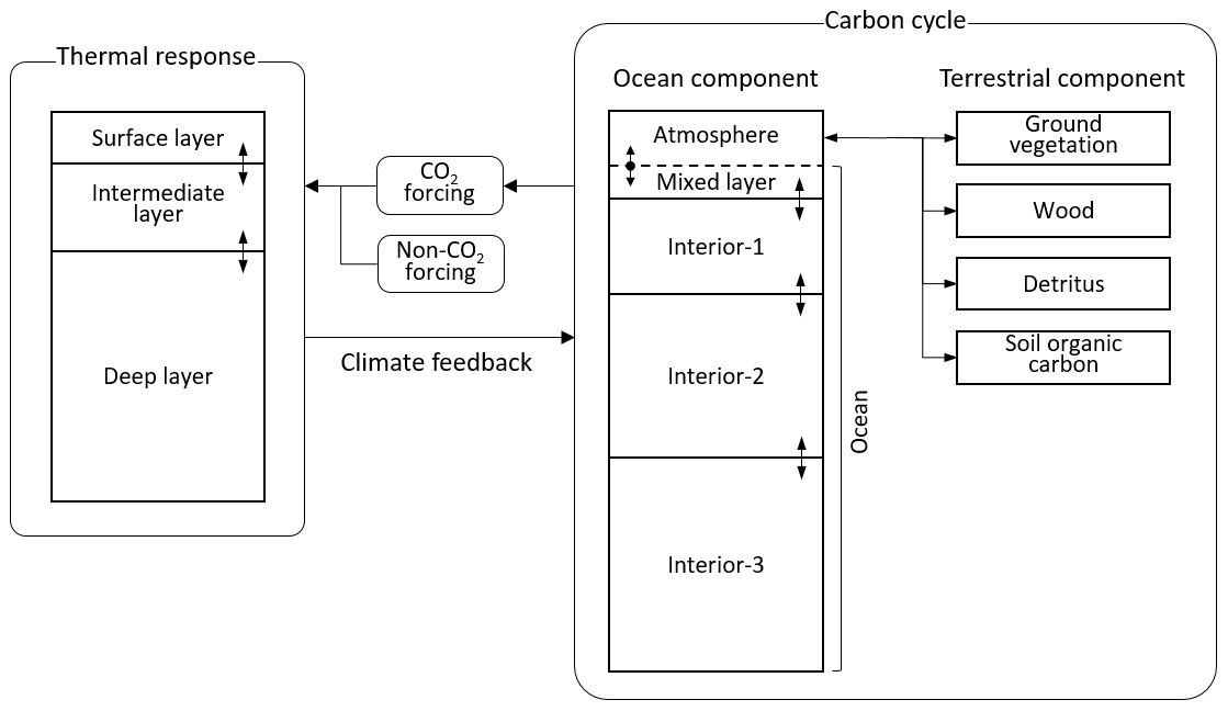
Figure 1Schematic diagram of the box models equivalent to the MCE's impulse response models. Bidirectional arrows represent heat and carbon fluxes within each module of the thermal response and carbon cycle. The two modules are connected through CO2 forcing and climate feedback mechanisms.
2.1 Impulse response models
The MCE model is essentially built on impulse response functions for the fraction of the total CO2 emitted that remains in the atmosphere (termed the airborne fraction), the decay of land carbon accumulated by the CO2 fertilization effect, and temperature change to radiative forcing of CO2 and other forcing agents. Under the linear response assumption with regard to input forcing F, an impulse response model (IRM) expresses the time change of a response variable x by a convolution integral:
where t is time, and the sum of exponentials is an impulse response function with parameters Ai and τi denoting the ith component of the response amplitude and time constant, respectively. The time derivative of this equation is given by
or an equivalent box model form that is converted into the original IRM through Laplace transform or eigenfunction expansion. The time derivative implemented in the MCE uses an IRM form for land carbon decay and temperature change and a box model form for the airborne fraction to address partitioning of excess carbon between the atmosphere and ocean mixed layer. Figure 1 illustrates the MCE's components in a box model form representing heat or carbon reservoirs. Since each component is formulated on its own impulse response functions, the boxes are separately defined between the thermal response and carbon cycle modules.
The IRM for the airborne fraction defines five components, one of which has an infinity time constant, paired with an amplitude corresponding to an asymptotic long-term fraction. In the current configuration, the remaining four time constants are fixed at 236.5, 59.52, 12.17, and 1.271 years, adjusted to a specific three-dimensional ocean carbon cycle model in Hooss et al. (2001). The corresponding amplitudes assume perturbations at reference values of 0.24, 0.21, 0.25, and 0.1, respectively, with a reference long-term airborne fraction of 0.20. These reference values and perturbation ranges are set empirically so that resulting carbon budgets – cumulative land and ocean CO2 uptake – agree with those of historical observations and CMIP experiments.
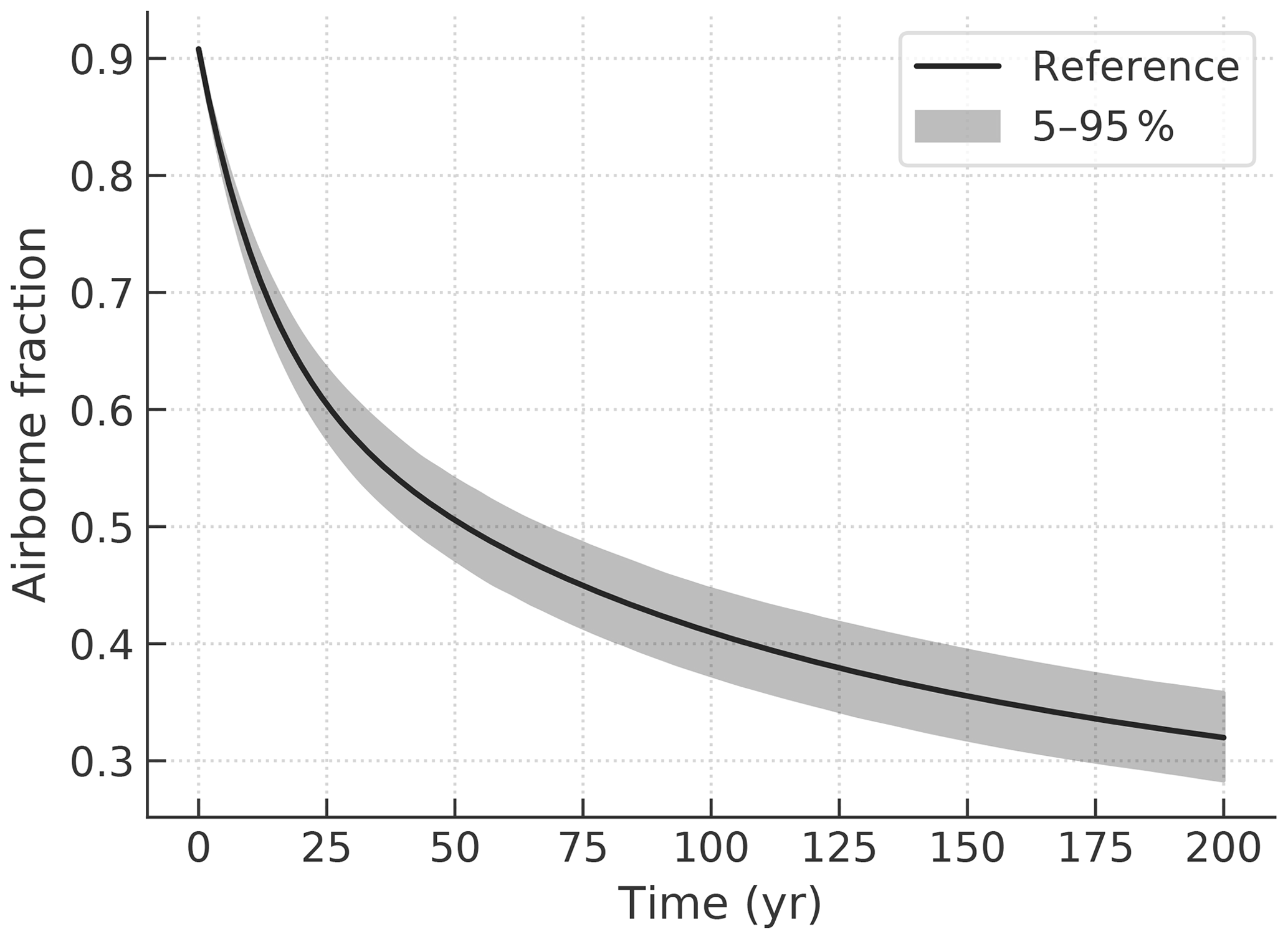
Figure 2Response of the airborne fraction to an initial input of 100 Gt C without land CO2 uptake and climate feedback. The line shows the case of reference amplitudes, and shading shows the range of the 5th–95th percentiles of the Prior ensemble, which is described in Sect. 3.1.
As described below, IRM parameters are converted into a set of parameters for an equivalent box model dealing with carbon exchange between four layers. In this conversion, the response of the shortest timescale component is interpreted as equilibration between the atmosphere and ocean mixed layer, which are combined into a composite layer in the box model, as shown in the ocean carbon cycle in Fig. 1. Figure 2 shows response to an idealized instantaneous input of 100 Gt C without land carbon uptake and climate feedback. In this case, the airborne fraction decreases from 0.9 to a long-term equilibrium of about 0.2 at a gradually decreasing rate. The asymptotic long-term airborne fraction is slightly greater than an assumed value, depending on the size of pulse input, due to the buffering mechanism of seawater.
The IRM for land carbon defines four carbon pools, representing ground vegetation, wood, detritus, and soil organic carbon, with distinct overturning times (τi). The forcing term (F) is net primary production (NPP) enhanced by the effect of CO2 fertilization, generally expressed by βLN0, where βL is a fertilization factor that depends on the atmospheric CO2 concentration, and N0 is base annual NPP (Gt C yr−1). The response amplitude (Ai) is rewritten as , where denotes a decay flux after an initial carbon input. Based on Joos et al. (1996), the IRM parameters of the four carbon pools are set to 2.9, 20, 2.2, and 100 years for τi and 0.70211, 0.013414, −0.71846, and 0.0029323 yr−1 for , respectively. Figure 3 illustrates response to unit forcing in this configuration.
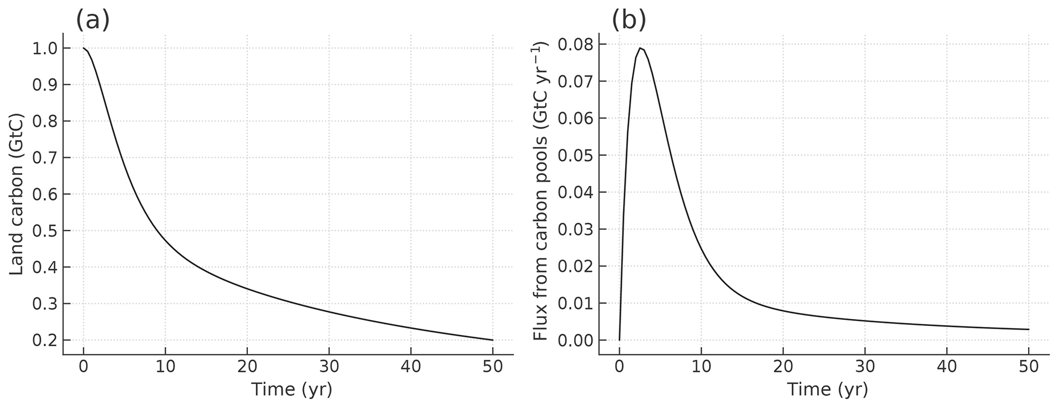
Figure 3Response of land carbon to instantaneous unit input (a) and accompanying flux from carbon pools (b).
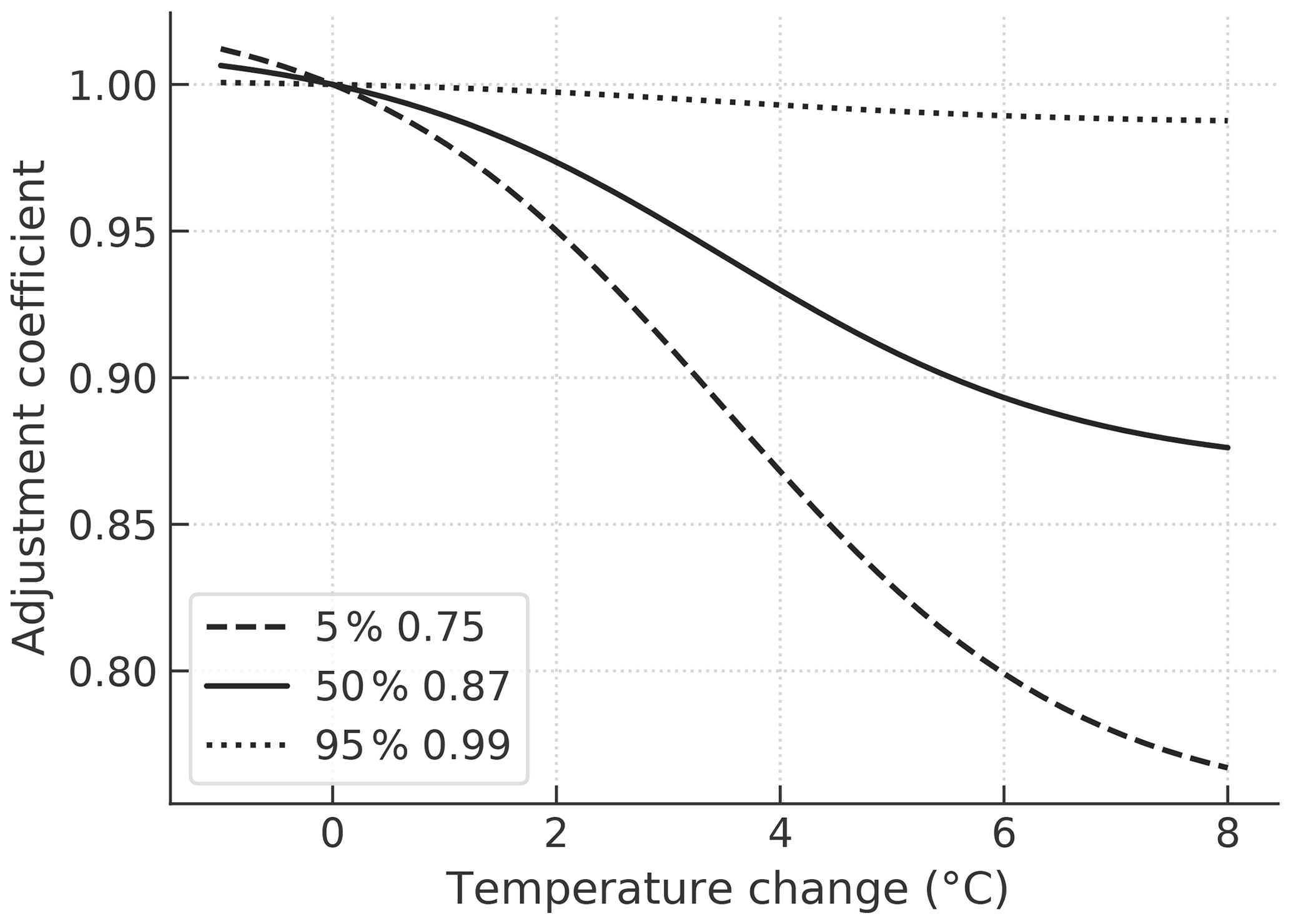
Figure 4Adjustment coefficient as a function of surface temperature change to multiply the time constants for the decay of wood and soil organic matter. The three curves are functions corresponding to the 5th, 50th, and 95th percentiles of the Prior ensemble, which is described in Sect. 3.1, with different asymptotic minimum values, as described in the legend. The temperature at which a curve has the maximum gradient is fixed at 3.5 ∘C.
In addition, the MCE deals with temperature dependency for the time constants of wood and soil organic carbon, indicating the tendency for warming to accelerate the decomposition of organic matter. This is one of the climate–carbon cycle feedback processes and is implemented with an adjustment coefficient varied along a logistic curve with respect to surface warming, as illustrated in Fig. 4. This scheme has a parameter to control the asymptotic minimum value of the coefficient. The figure shows three curves with different control parameters, corresponding to the 5th, 50th, and 95th percentiles of the Prior ensemble, which is described in Sect. 3.1, adjusted to be consistent with the variation of CMIP Earth system models (ESMs). In the IRM form, land accumulated carbon is proportional to , expressing the remaining carbon at an equilibrium state under unit continuous input, and the decrease in the time constants affects accumulated carbon quadratically.
The IRM of the temperature change defines three components with typical time constants of approximately 1, 10, and >100 years. Although the temperature response is usually well represented by two separated time constants of approximately 4 and >100 years (e.g., Held et al., 2010; Geoffroy et al., 2013), dividing fast response is advantageous when considering instantaneous forcing changes, such as volcanic eruptions (Gupta and Marshall, 2018) and geoengineering mitigation, and using three time constants appears to be practically optimal choice (Cummins et al., 2020). Separating the intermediate time constant is also beneficial for representing a pattern effect – warming response affected on a decadal or multi-decadal timescale by the changing pattern of surface warming (e.g., Andrews et al., 2015). The response amplitude is rewritten by , where is normalized so that the component sum is unity, and λ is the climate feedback parameter (W m−2 ∘C−1), defined as the derivative of the outgoing thermal flux with respect to temperature change. These IRM parameters can be adjusted to emulate individual CMIP models with sufficient accuracy, as demonstrated in Tsutsui (2020), which serves a basis to build a perturbed parameter ensemble.
2.2 Carbon uptake over ocean
The box model converted from the IRM for the airborne fraction is as follows:
where ck is the amount of excess carbon in layer k, hk is the layer depth, ηk is the exchange coefficient between layer k−1 and layer k, e is anthropogenic emissions, and f is natural uptake over land. The parameters hk and ηk are set through numerical optimization for the box model to be equivalent to the IRM form. The top layer, indexed with 0, is the composite atmosphere–ocean mixed layer, and the three subsurface layers are indexed with 1, 2, and 3 in the order of ocean depth. The amount of excess carbon in the top layer (c0) is partitioned into atmospheric and ocean components, denoted by ca and cs, subject to chemical equilibrium at the ocean surface. The carbon exchange between the top layer and the first subsurface is expressed in terms of cs.
For a given time series of CO2 emissions (emission-driven) or atmospheric CO2 concentrations (concentration-driven), time integration is performed. In the latter case, c0 and its partition within the composite layer are diagnostically determined, and the top layer equation is dropped.
The partition of c0 is solved through numerical computation with regard to hydrogen ion concentration associated with changes in dissolved inorganic carbon concentration (DIC) under the assumption of constant alkalinity (Alk). DIC, defined as the sum of [CO2], [], and [], where [x] denotes the concentration of a substance x (mol L−1), is expressed as
where K1 and K2 are equilibrium constants for bicarbonate and carbonate, defined as and . [CO2], defined as the sum of [CO2(aq)] and [H2CO3(aq)], is related to the partial pressure of CO2 (pCO2) with equilibrium constant K0, as in . Alkalinity, here considering borate ions as well as bicarbonate and carbonate ions, is represented as
where BT is total borate concentration , and Kb and Kw are equilibrium constants for borate and water, defined as and .
The values of Alk, BT, and the equilibrium constants of K0, K1, K2, Kb, and Kw are set based on Dickson et al. (2007). The equilibrium constants depend on water temperature, and carbon uptake decreases with temperature, representing a climate–carbon cycle feedback process. This temperature dependency is implemented as a linear regression for empirical expressions, as shown in Fig. 5.
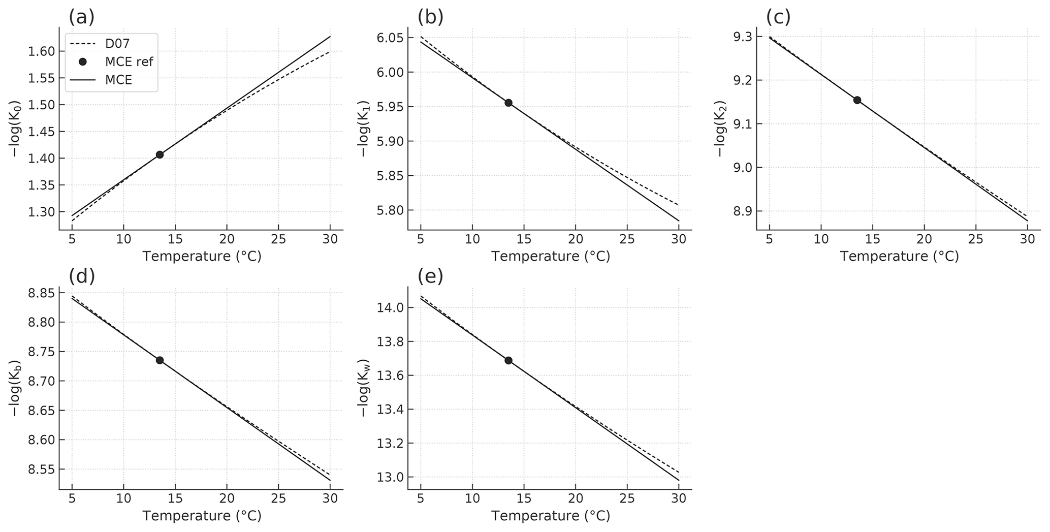
Figure 5Temperature-dependent equilibrium constants of K0, K1, K2, Kb, and Kw (a–e) in the MCE model (solid lines), which approximate empirical expressions in Dickson et al. (2007) (D07, dotted lines). Values at a reference seawater temperature of 13.5 ∘C (dots) are assigned to those in the MCE's preindustrial state.
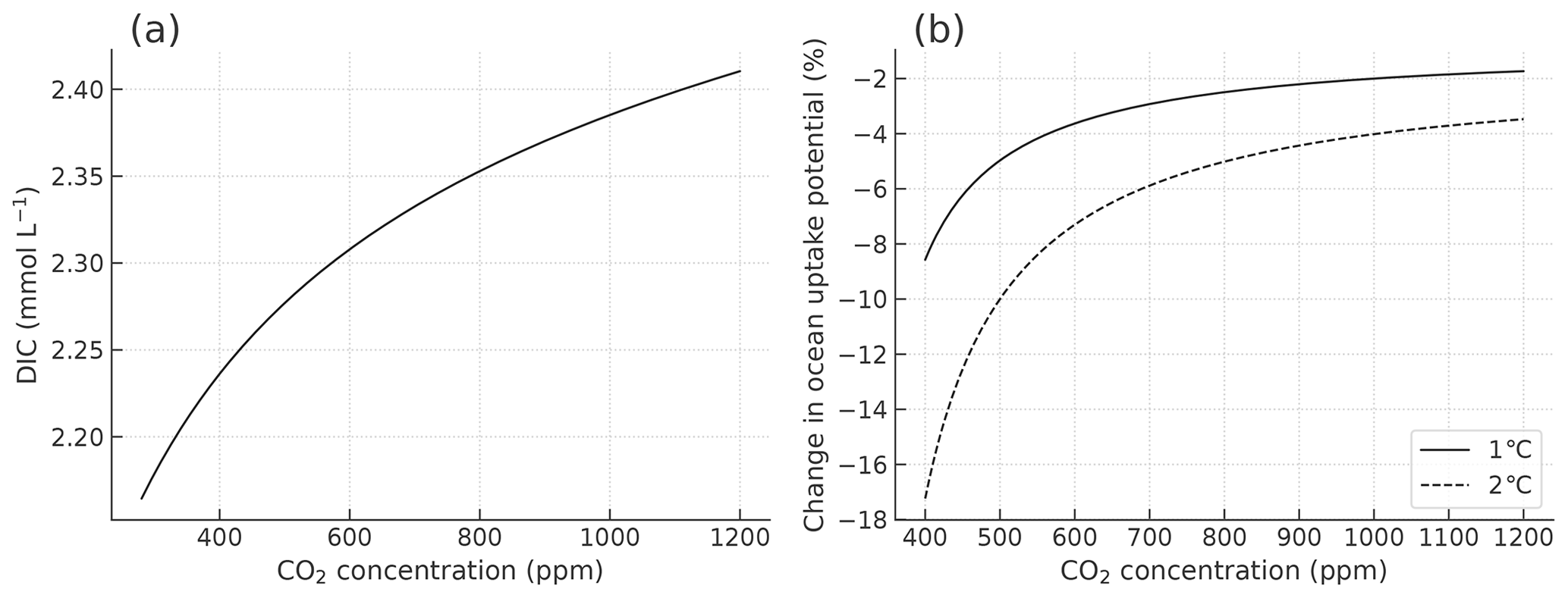
Figure 6DIC in the ocean mixed layer as a function of atmospheric CO2 concentration (a) and changes in ocean carbon uptake potential, measured by the increase in DIC from preindustrial levels, due to 1 and 2 ∘C warming (b). The preindustrial CO2 concentration is assumed to be 284.317 ppm, and preindustrial DIC is about 2.17 mmol L−1.
The amount of excess carbon that can be accumulated in the ocean is proportional to a change in DIC from its preindustrial value. This carbon uptake potential and its temperature dependency are illustrated in Fig. 6. CO2-induced global warming increases the airborne fraction in two ways – through the buffering mechanism of seawater and through temperature dependency of chemical equilibrium. The former is shown as a decreasing change rate of the DIC with regard to atmospheric CO2 concentration (Fig. 6a), while the latter is shown as a reduction in rates of carbon uptake potential with temperature, which also depends on the concentration (Fig. 6b). The reduction rate is approximately proportional to the warming level, typically about 4 % per 1 ∘C at doubling CO2.
2.3 CO2 fertilization
The land carbon uptake term f in Eq. (3) is calculated from Eq. (2), rewritten as
where cbi is the ith component of accumulated carbon by CO2 fertilization. The base NPP (N0) is set to 60 Gt C yr−1 and the fertilization factor (βL) is formulated with a sigmoid curve with regard to CO2 concentration C(t), as described in Meinshausen et al. (2011). This implementation is connected to a conventional logarithmic formula,
such that the sigmoid and logarithmic curves are equal in terms of an increase ratio at 680 ppm relative to 340 ppm, and the latter factor is used as a control parameter. Figure 7 illustrates three curves with different control parameters in the MCE model.
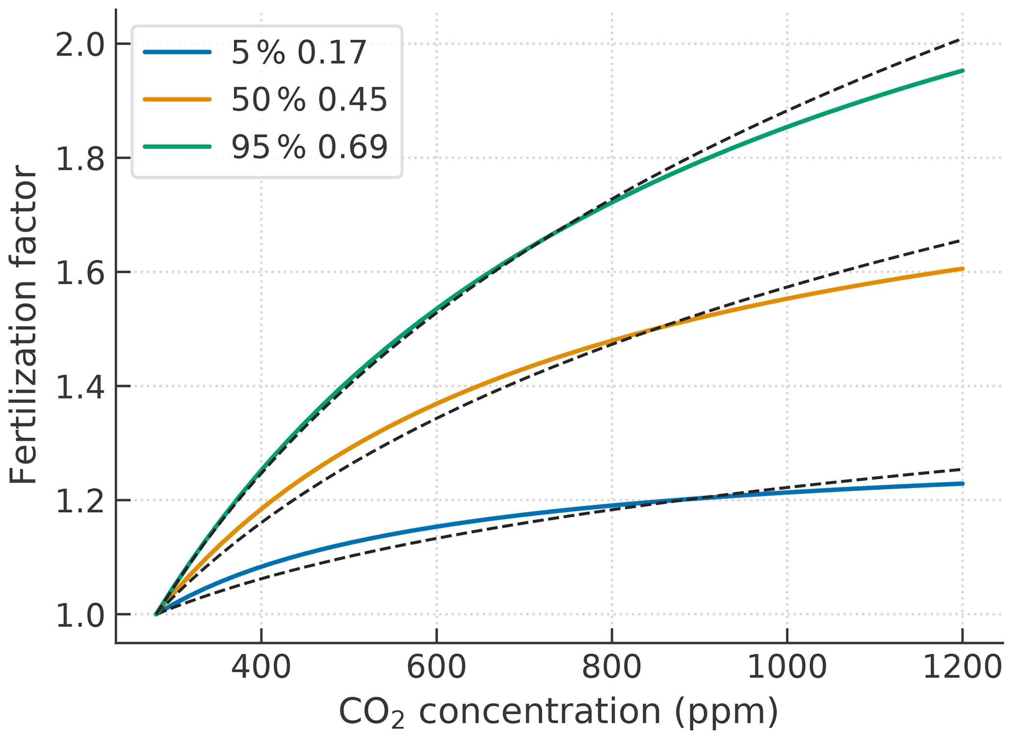
Figure 7CO2 fertilization factor as a function of atmospheric CO2 concentration with different control parameters () of 0.17, 0.45, and 0.69, corresponding to the 5th, 50th, and 95th percentiles of the Prior ensemble described in Sect. 3.1. The colored lines show sigmoid curves used in the MCE model, and the black dashed lines show reference logarithmic curves.
2.4 Effective radiative forcing
The forcing term in the IRM for temperature change is assumed to be effective radiative forcing (ERF), defined as top-of-atmosphere (TOA) radiative imbalance due to a change in a forcing agent through rapid adjustments in the stratosphere and troposphere prior to a response in surface temperature (Myhre et al., 2013; Sherwood et al., 2015). Forcing, defined as such, serves as a good predictor of surface temperature change.
CO2 forcing is evaluated with the following quadratic formula in terms of the logarithm of CO2 concentration:
where x is the ratio of CO2 concentrations to a preindustrial level, αC is a scaling parameter (W m−2), and βC is an amplification factor defined as . This scheme was presented in Tsutsui (2017) to emulate the CMIP's core CO2 increase experiments for instantaneous quadrupling and 1 %-per-year increase, referred to as abrupt-4xCO2 and 1pctCO2, respectively. Thus, the scheme is valid in the range of . The two control parameters are diagnosed consistently with IRM parameters for individual CMIP models (Tsutsui, 2020). The current diagnosing procedure solves numerical optimization to approximate the first 150-year and 140-year time series from abrupt-4xCO2 and 1pctCO2 experiments, respectively, in terms of TOA energy imbalance and the surface air temperature anomaly, respectively. The quadratic term is activated when the concentration exceeds 2 times (x>2), and βC is set to unity in the range x≤2 so that FC is equivalent to . The forcing amplification is expected to be valid in the range x≤4 and the quadratic term is dropped beyond a level of 4 times. Figure 8 illustrates example outputs of the CO2 forcing scheme in a range of 5th–95th percentiles of the Prior ensemble for control parameters.
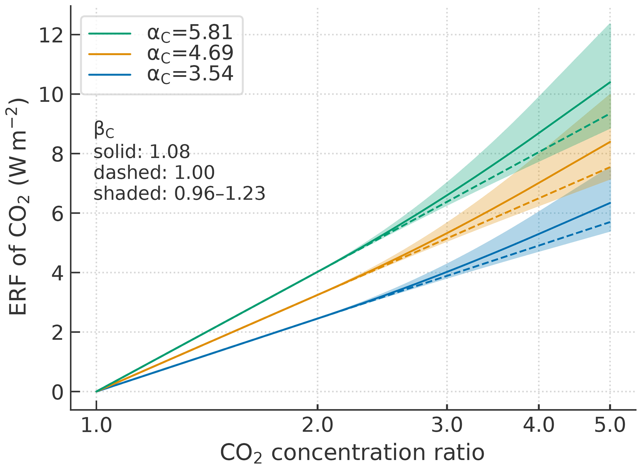
Figure 8Effective radiative forcing (ERF) of CO2 as a function of the ratio of CO2 concentrations to a preindustrial level. The scaling parameter αC is set to three different values, corresponding to the 5th, 50th, and 95th percentiles of the Prior ensemble described in Sect. 3.1. For each αC value, the amplification factor βC is varied between the 5th and 95th percentiles (shaded area) and is set to two specific values of the 50th percentile (solid line) and unity (dashed line, no amplification).
The forcing of CH4 and N2O is evaluated with the expressions given in Etminan et al. (2016). The forcing of halogenated gases is simply calculated as changes in concentration from preindustrial levels multiplied by radiative efficiencies assessed in the latest IPCC report (at the time of this paper preparation AR5; Myhre et al., 2013).
The current MCE model does not support non-CO2 gas cycles and ERF schemes for other forcing agents, such as aerosols, tropospheric and stratospheric ozone, solar radiation, and volcanic eruptions. Experiments considering non-CO2 forcing require prescribed concentrations for long-lived GHGs and prescribed ERF for others.
2.5 Parameter sampling
Probabilistic runs use an ensemble of perturbed model parameters designed to encompass the variation of multiple CMIP models with additional constraints with regard to assessed ranges of key climate indicators. In general, a series of candidate values of an uncertain parameter is generated from its statistical model and, if necessary, sampled from the series with an acceptance algorithm for given constraints. The latter process is Bayesian updating from a prior probability distribution to a posterior and uses a Metropolis–Hastings (MH) independence sampler here. As mentioned above, uncertain parameters include IRM amplitudes for the airborne fraction, control parameters for land carbon decay timescales and CO2 fertilization, IRM parameters for temperature change, and control parameters for the CO2 forcing scheme.
In a Bayesian framework, some difficulties arise from setting appropriate prior distributions and dealing with large-dimension likelihood functions. Although the latter can be avoided by using the Markov chain Monte Carlo (MCMC) approach, its implementation, typically based on the MH algorithm, is not necessarily straightforward in exploring a large-dimension parameter space with the detailed balance that underlies MCMC. One of the relevant issues is sampling efficiency. Goodwin and Cael (2021), for example, generated a prior by varying a set of ∼25 model parameters independently with a very large size of ∼109 and constrained it by an acceptance algorithm with an observation-based likelihood function. Although the prior ensemble size can be reduced by improving the acceptance algorithm (Goodwin, 2021), it appears to need ∼107 to get a posterior for typical application, such as climate sensitivity estimation and probabilistic climate projections.
The current MCE approach is one way to deal with the above difficulties. Setting a prior with statistical models representing a CMIP multi-model ensemble allows the use of an efficient MH independence sampler, with the size of a prior series for typical applications expected to be ∼104 or at most ∼105. It is also convenient that this sampler is free from adjustment, unlike random-walk-based MCMC implementation that requires step-size adjustment. One thing to note is that the independence sampler is suitable when the proposed prior series encompasses the target posterior series, and the acceptance rate of sampling is high to some extent. However, this requirement is not met for the case presented below. This problem is addressed in the implementation of the MH algorithm in Sect. 3 and further discussed in Sect. 4.
The carbon cycle parameters are individually generated from a uniform distribution with a given mean and perturbation range. The means and ranges are determined on a trial basis so that ranges of carbon budgets in historical and scenario experiments are consistent with those from multiple CMIP ESMs. Since the sum of IRM amplitudes for the airborne fraction is unity, their perturbed values are normalized as such, subject to a modified distribution with more samples about the mean resulting from the operation.
The temperature response and CO2 forcing parameters are synthetically generated from a multivariate normal distribution reflecting the variation of multiple CMIP AOGCMs. The IRM for temperature change has three pairs of time constant (τi) and dimensional amplitude (Ai), and the CO2 forcing scheme has two control parameters (αC and βC). A total of eight parameters have been diagnosed for each of the multiple CMIP models, revealing characteristic covariance structures, such as a noticeable negative correlation between feedback strength () and a realized warming fraction (typically TCR-to-ECS ratio), as well as a weakly negative correlation between the forcing scale (αC) and feedback strength (Tsutsui, 2020). The multivariate normal distribution is built on principal components (PCs) of these diagnosed parameters, as described in Tsutsui (2017).
The eight parameters to be fed into PC analysis can include some derived parameters from the following expressions:
where ECS is defined using a diagnosed forcing of CO2 doubling, while ECSG uses CO2 quadrupling with a factor of 0.5 as in Gregory et al. (2004). Equation (16) is derived from time integration of Eq. (1) to the 70th year (t70) along a 1 %-per-year increasing path that defines TCR. One possible set consists of TCR, , , τ0, τ1, τ2, αC, and βC, applied with logarithmic transformation, except for αC. This set was adopted in the experiments described below. The logarithmic transformation is intended to allow fair normality of PC scores as a basis for fitting a multivariate normal distribution and to make generated candidates positive.
Probabilistic runs can also use different scaling factors to adjust individual non-CO2 ERF time series. This is a simple implementation to deal with non-CO2 forcing uncertainties, typically assessed as a range at a reference time point. The scaling factor is perturbed with a suitable statistical model fitted to the range.
All uncertain parameters and ERF scaling parameters are not necessarily independent. The current sampling procedure incorporates covariance between the eight parameters relevant to temperature change in response to CO2 forcing. However, the procedure assumes no other correlations, implying that uncertainties of the CO2-induced temperature response are independent from those of the carbon cycle and non-CO2 forcing.
3.1 Scenario experiments
To demonstrate a typical application of the MCE model, a number of scenario experiments that mirror those of CMIP6 were conducted, including idealized abrupt-4xCO2 and 1pctCO2, as well as historical–future scenarios based on the Shared Socioeconomic Pathways (SSPs; Riahi et al., 2017). In the latter experiments, the model was initialized for the year 1850 and driven with GHG concentrations and other prescribed ERF, both provided from the RCMIP (Nicholls et al., 2020).
For each scenario, two sets of 600-member ensemble runs were conducted; one was perturbed to be consistent with a CMIP multi-model ensemble and the other was further constrained according to the RCMIP Phase 2 protocol (Nicholls et al., 2021), here labeled Prior and Constrained, respectively. Prior refers to 25 CMIP5 and 38 CMIP6 AOGCMs for the PC analysis input and to 8 CMIP5 and 11 CMIP6 ESMs diagnosed in Arora et al. (2020) for simulated carbon budgets in the 1pctCO2 experiment. Diagnosed forcing and response parameters of the multiple AOGCMs are presented in the MCE's code repository.
The uncertain carbon cycle parameters for Prior were generated from the abovementioned statistical models, as shown in Figs. 1, 3, and 6, and were processed by the MH sampler to constrain accumulated land carbon at doubling CO2 along the 1 %-per-year pathway. In this case, 1pctCO2 scenario runs with a set of proposed parameters were conducted to obtain data fed into the sampler. This single constraint was selected as it works inclusively for other relevant constraints through a trade-off relationship between ocean and land in terms of accumulated carbon.
RCMIP Phase 2 defines a number of constraints for climate indicators, including ERF levels, carbon budgets, recent warming trends, and climate sensitivity metrics of ECS, TCR, and transient climate response to cumulative CO2 emissions (TCRE). Here, TCRE is defined as the ratio of the TCR to implied cumulative CO2 emissions at the time of CO2 doubling along the same 1 %-per-year trajectory as that for TCR. These constraints use literature-based assessed ranges, referred to as a “proxy assessment”, to distinguish these from the formal IPCC assessment. The Constrained uncertain parameters were sampled from those of Prior through a sequence of the MH sampler with a subset of RCMIP constraints, as follows: (1) CO2 ERF in 2014 relative to 1750 evaluated in Smith et al. (2020), (2) TCR estimated in Tokarska et al. (2020, Table S3, both constrained), and (3) GMST in the period 1961–1990 relative to the period 2000–2019 from the HadCRUT.4.6.0.0 dataset (Morice et al., 2012) and ocean heat content (OHC) in 2018 relative to 1971 from the dataset of von Schuckmann et al. (2020). In this case, in addition to 1pctCO2 runs, historical scenario runs with a set of proposed parameters were conducted to obtain data fed into the sampler.
The IRM for temperature change is transformed into a three-layer heat exchange model in physical space (Fig. 1). The top layer is representative of fast-responding Earth system components – the atmosphere and Earth's surface including a part of the ocean mixed layer. However, when diagnosing the CO2 forcing and response parameters, the top layer temperature was treated as global mean surface air temperature (GSAT) in practice. As in HadCRUT GMST was defined as a surface air–ocean blended temperature change; here, a factor of 1.04 was used to convert observed GMST change into the MCE's GSAT change. Likewise, as the MCE's three layers cannot be allocated to specific climate system components, a factor of 1.08 was used to convert observed OHC change into the MCE's total heat content change.
Besides CO2 forcing, the RCMIP constraints include the ranges of non-CO2 forcing over a historical period for CH4, N2O, halocarbons (aggregated into “Montreal gases” – CFCs, HCFCs, halons – and other “F gases” – HFCs, PFCs, SF6), aerosols (aggregated), tropospheric ozone, stratospheric ozone, stratospheric water vapor from CH4, and albedo change due to land use and black carbon aerosols on snow and ice. Ranges are based on AR5 (Myhre et al., 2013), except for those for CH4 and aerosols, which consider recent updates (Etminan et al., 2016; Smith et al., 2020). To incorporate these uncertainty ranges in historical-future scenarios, the scaling factors to adjust individual non-CO2 ERF time series were perturbed using normal or skewed normal distributions fitted to the prescribed ranges.
The RCMIP constraints are provided as likely ranges and optionally very likely ranges, corresponding to 17 %–83 % and 5 %–95 % according to the IPCC's likelihood terms. These ranges were applied to generate uncertain parameter proposals and to build the MH sampler requiring probability densities for a target distribution.
Although a number of indicators were prepared for the RCMIP constraints, a very limited number of those were used here, partly because the prior was designed to match some of them like the forcing constraints and partly because the proxy assessment ranges are not necessarily consistent with each other. The sequence of the MH sampler for the above three items, which relaxes the detailed balance required for MCMC, was established to deal with those constraints and needs to be improved using fully consistent assessment ranges.
Other details of the constraining procedures and experimental specifications are provided in the MCE's code repository (see “Code and data availability” at the end).
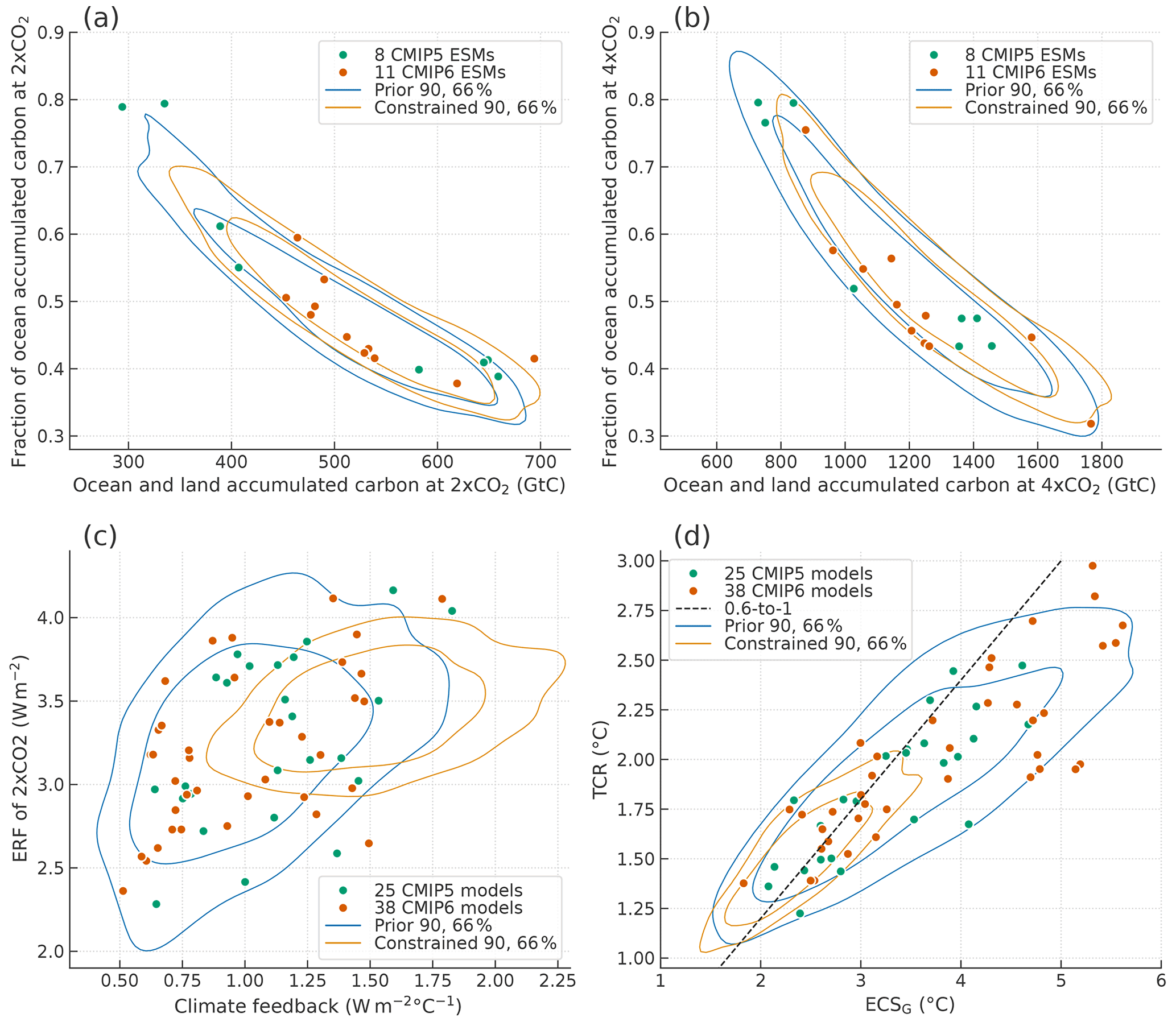
Figure 9Relationships between key indicators associated with carbon budget and climate sensitivity in comparison with CMIP models. Contours indicate kernel density levels at which the circles cover 90 % and 66 % of members. The legend indicates the number of the CMIP models. (a) The fraction of ocean accumulated carbon as well as ocean and land totals in the 70th year of 1pctCO2. (b) Same as panel (a), but in the 140th year. (c) Effective radiative forcing (ERF) of CO2 doubling and climate feedback parameter. (d) Transient climate response (TCR) and equilibrium climate sensitivity diagnosed from abrupt-4xCO2 (ECSG). The dashed line is located where the ratio of TCR to ECSG is 0.6 as a reference.
3.2 Results: climate indicators
Figure 9 illustrates relationships between key indicators associated with the carbon budget and climate sensitivity of the two ensembles in comparison with the CMIP models. The carbon budget is measured by the amount of accumulated carbon and its allocation to ocean and land reservoirs. Here, total accumulation and the ocean allocation ratio at doubling and quadrupling CO2 levels are used as key indicators. The CMIP ESMs indicate a clear negative correlation between the two quantities (Fig. 9a and b), reflecting much greater uncertainties relating to land carbon. This feature is well represented by the MCE parameter ensembles. Although there are some model differences between CMIP5 and CMIP6 eras, such as a reduced model spread in the latter associated with nitrogen cycle implementation (Arora et al., 2020), the MCE ensembles currently do not distinguish between the two. The carbon indicators of the Constrained ensemble do not differ significantly from those of Prior but are distributed toward higher total accumulations, which is attributed to warming differences that affect carbon cycle–climate feedbacks.
In contrast, climate sensitivity differences are most prominent and well characterized with key indicators' distributions on two-dimensional domains: the ERF of CO2 doubling derived from αC vs. the climate feedback parameter (λ) (Fig. 9c) and TCR vs. ECSG (Fig. 9d). While the Prior distributions cover the CMIP AOGCMs effectively, the Constrained distributions are confined to lower sensitivity values – greater λ and smaller TCR and ECSG, which is attributed to the observed GMST and OHC constraints. The Prior distribution of the CO2 forcing agrees well with the CMIP distribution, which shows a weakly positive correlation with the climate feedback parameter. In contrast, the Constrained forcing levels are confined to an upper half of the CMIP AOGCMs, which is attributed to the historical CO2 forcing constraint, and the forcing–feedback correlation becomes weak. Transient sensitivity is not necessarily proportional to equilibrium sensitivity, and greater CMIP6 sensitivity is more evident in ECSG than in TCR. The inherent relationship between feedback strength and response timescales is responsible for the tendency, together with the forcing amplification effect represented by βC. The PC-analysis-based statistical model captures such covariance structure effectively.
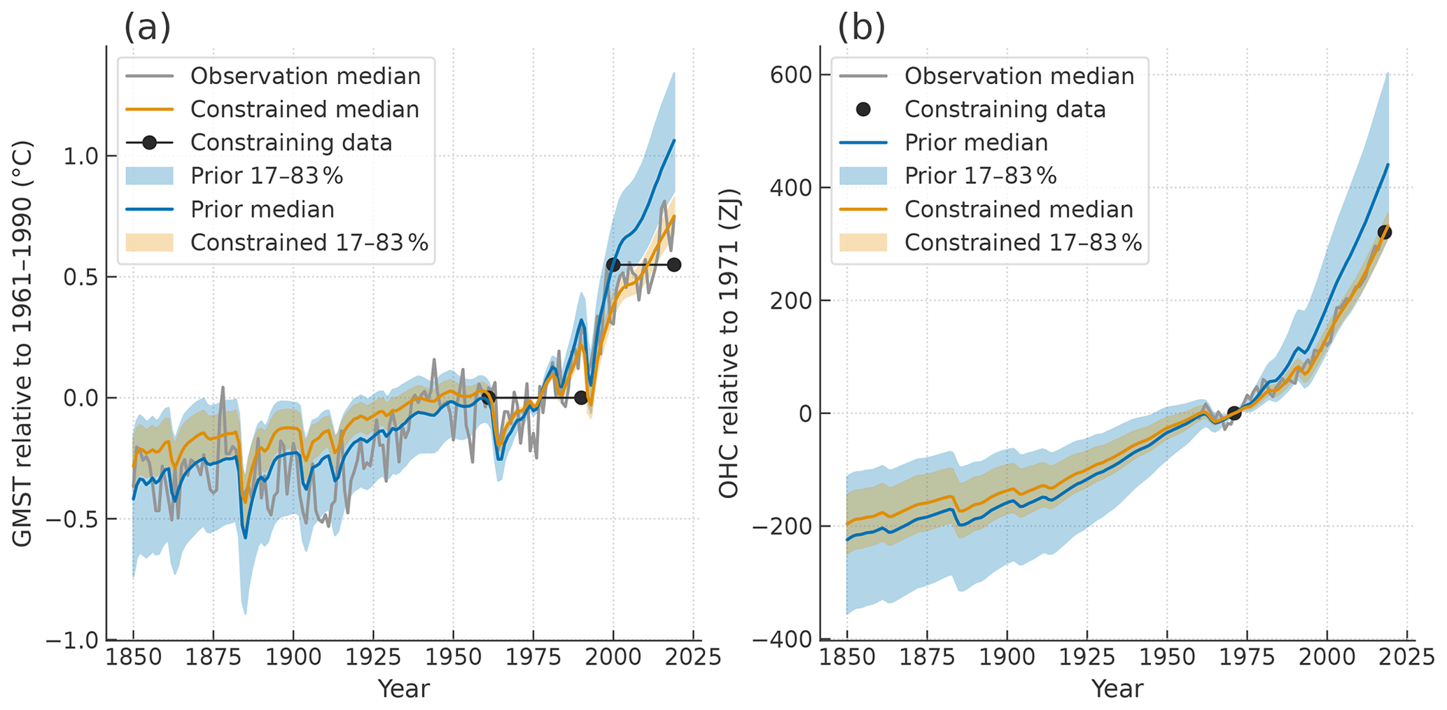
Figure 10(a) Historical global mean surface temperature (GMST) relative to 1961–1990 and (b) historical ocean heat content (OHC) relative to 1971 in the period 1850–2019 compared with observation data from HadCRUT4.6.0.0 for GMST and von Schuckmann et al. (2020) for OHC. The black dots indicate the levels in two different periods or years used for the observation constraints.
Figure 10 illustrates historical GMST and OHC of the MCE's two ensembles in comparison with their observations, from which constraining data are considered for recent warming trends. In the figure, the time series are adjusted relative to the reference period 1961–1990 for GMST and the reference year 1971 for OHC. While the Prior series are well above the observed warming during the target period 2000–2019 for GMST and during the target year 2018 for OHC, the Constrained series agree well with recent trends. The observation-based constraining results in lower climate sensitivity in the latter ensemble. However, considerable uncertainties remain with regard to longer trends and unforced climate variability. In an earlier period, observed GMST was rather close to Prior, and the Constrained trend appears to be underestimated. The OHC trend cannot be validated owing to its limited observation period. Assessment of forced response in the historical period, which is currently not available, would allow more reliable parameter sampling. Some variation in the historical forcing time series, in particular for aerosols (Smith et al., 2021), would also be worth exploring.
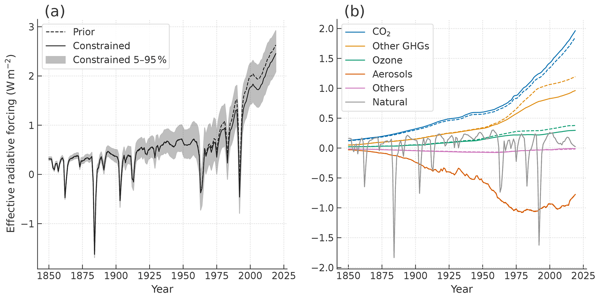
Figure 11Historical effective radiative forcing (ERF) in the period 1850–2019 for total ERF (a) and aggregated components (b). The ensembles' medians are shown by lines, and the 5 %–95 % range of the Constrained ensemble is shown for the total by shading.
The greater warming in Prior is not only due to its greater climate sensitivity, but also partly due to non-CO2 forcing differences, as shown in Fig. 11. The scaling factors of the non-CO2 forcing agents are independently perturbed in the Prior ensemble and probabilistically selected through the series of the MH sampler. Although the sampling process does not directly refer to forcing levels of non-CO2 agents, it can modify their distributions to be consistent with other constraints. This modification is found for non-CO2 GHGs and ozone time series (Fig. 11b), and the most dominant contribution is of Montreal gases (not shown). The ERF of Montreal gases rapidly increases from the 1960s and levels off from the 1990s, and the sampling results imply that this tendency is not consistent with the recent warming trend. Total ERF fluctuates with changes in solar irradiance and volcanic eruptions, for which the RCMIP's prescribed forcing was used without their efficacy uncertainties.
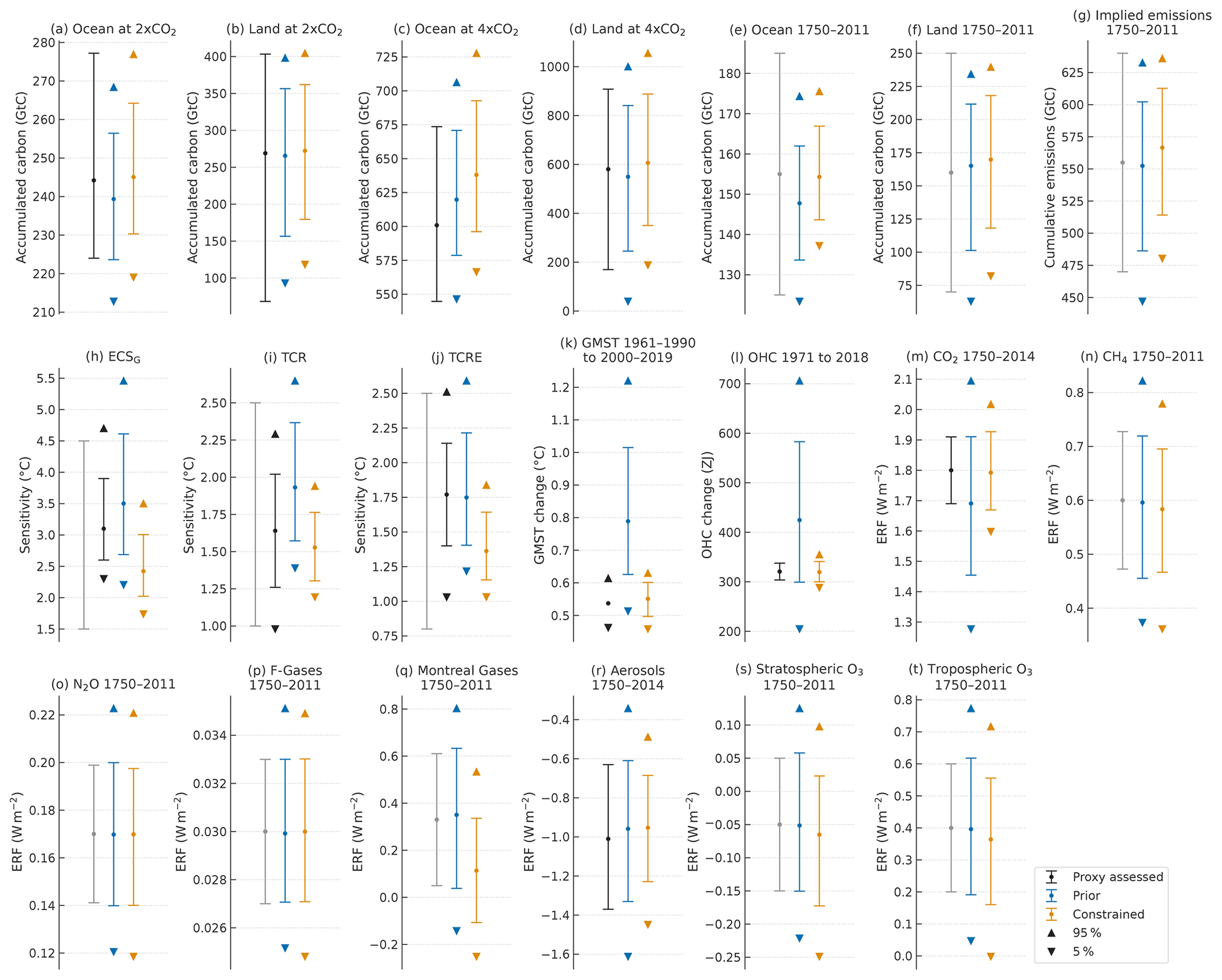
Figure 12Distributions of climate indicators: (a) accumulated carbon over ocean at doubling CO2 in 1pctCO2; (b) same as (a) but over land; (c) same as (a) but at quadrupling CO2; (d) same as (c) but over land; (e) accumulated carbon over ocean in 1750–2011; (f) same as (e) but over land; (g) implied cumulative emissions in 1750–2011; (h) equilibrium climate sensitivity diagnosed with CO2 quadrupling forcing (ECSG); (i) transient climate response (TCR); (j) transient climate response to 1000 Gt C cumulative CO2 emissions (TCRE); (k) global mean surface temperature (GMST, air–ocean blended) in 2000–2019 relative to 1961–1990; (l) ocean heat content (OHC) in 2018 relative to 1971; (m) effective radiative forcing (ERF) of CO2 in 2014 relative to 1750; (n) ERF of CH4 in 2011 relative to 1750; (o) same as (n) but of N2O; (p) same as (n) but of “Montreal gases” (CFCs, HCFCs, halons); (q) same as (n) but of “F gases” (HFCs, PFCs, SF6); (r) same as (m) but of aerosols; (s) same as (n) but of stratospheric O3; (t) same as (n) but of tropospheric O3. Error bars and pairs of triangle markers indicate likely ranges (17 %–83 %) and very likely ranges (5 %–95 %), respectively. The black and grey error bars indicate proxy assessment ranges and AR5-assessed ranges, respectively. The proxy ranges are based on 5 %–95 % ranges of the CMIP Earth system models in (a)–(d) but are otherwise taken from the RCMIP Phase 2 protocol that partly includes the AR5-assessed ranges.
Figure 12 displays the ranges of climate indicators from the two ensembles associated with the carbon cycle, climate sensitivity, warming trends, and historical ERF changes in comparison with their proxy assessment ranges. The consistency between modeled and proxy ranges can be most distinctively shown for warming trends by GMST and OHC changes (Fig. 12k and l), with Prior ranges substantially wider and higher than assessed ranges but comparable Constrained ranges. The consistency of sensitivity indicators, including TCRE (Fig. 12h–j), is complex because the proxy assessment ranges (black error bars) themselves are not necessarily consistent with each other, as discussed in the next section, and narrowed from the AR5-assessed ranges (grey error bars). Overall, consistency is better for Prior ranges, although Constrained ranges, which are considerably narrowed and lowered, are still within the AR5-assessed ranges. The ranges of the carbon cycle indicators (Fig. 12a–g), including accumulated carbon and implied cumulative emissions in the historical period 1750–2011, are not significantly different between the two ensembles and broadly agree with assessed ranges. Ensemble runs for the extended historical period starting from 1750 were conducted for calibration. The ranges of the ERF indicators (Fig. 12m–t) are consistent with assessed ranges, except for Prior CO2 and Constrained Montreal gases, as mentioned above. Other minor changes from Prior to Constrained include a reduced range for aerosols and lowered ranges for stratospheric and tropospheric ozone.
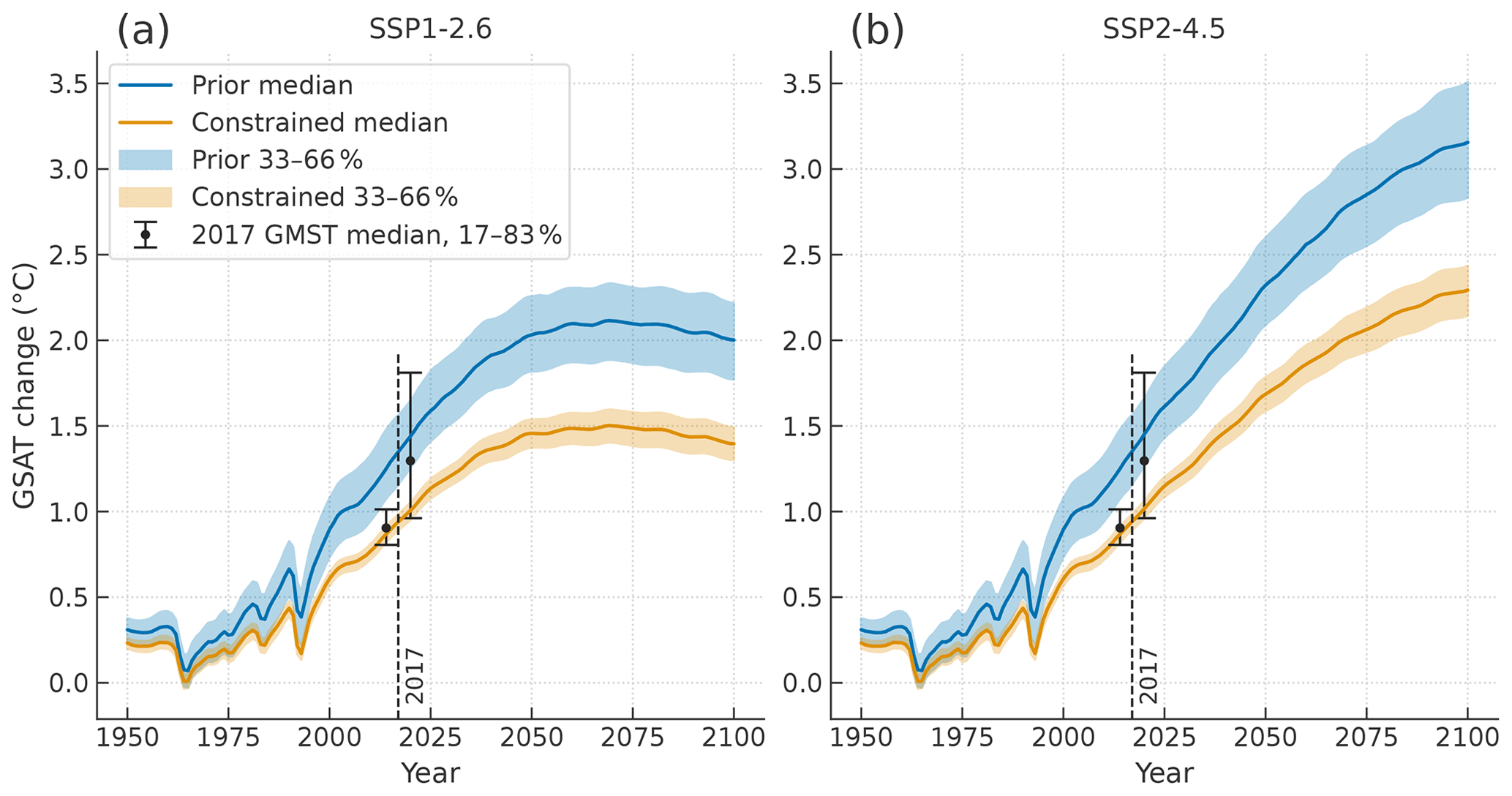
Figure 13Global mean surface air temperature (GSAT) changes relative to 1850–1900 in SSP1–2.6 (a) and SSP2–4.5 (b) scenarios from Prior and Constrained ensembles. Medians and 33 %–66 % ranges at each time point are shown by lines and shading. The error bars indicate medians and likely (17 %–83 %) ranges of global mean surface temperature (GMST, air–ocean blended) changes in 2017. For visual purposes the two error bars are slightly shifted from the reference year of 2017 on the horizontal axis.
3.3 Results: projected warming
Figure 13 illustrates temperature response in two SSP scenarios, SSP1–2.6 and SSP2–4.5, wherein warming is measured by an increase in global mean surface air temperature (GSAT) relative to 1850–1900, and the period up to 2100 is presented. In the scenario labeled SSPn-x.x, “n” (1–5 numbers) identifies different socioeconomic development pathways, and “x.x” expresses a nominal forcing level (W m−2) at the end of the 21st century. The shaded areas indicate 33 %–66 % ranges. The upper bound corresponds to the level to which warming is likely (66 %–100 %) to be limited at the time, while the lower bound corresponds to the level which warming is likely to exceed. These thresholds are shown in Table 1 for peak and end-of-century (end-21C) warming for eight SSP scenarios, wherein the end-21C period is set to 2081–2100 in accordance with the AR5.
Table 1Critical global mean surface air temperature (GSAT) change relative to 1850–1900 in different Shared Socioeconomic Pathway (SSP) scenarios. Warming levels at peak during the 21st century and averaged over the period 2081–2100 (end-21C) are shown for those likely to be limited (66th percentile) and likely to exceed (33rd percentile) from Prior and Constrained ensembles.
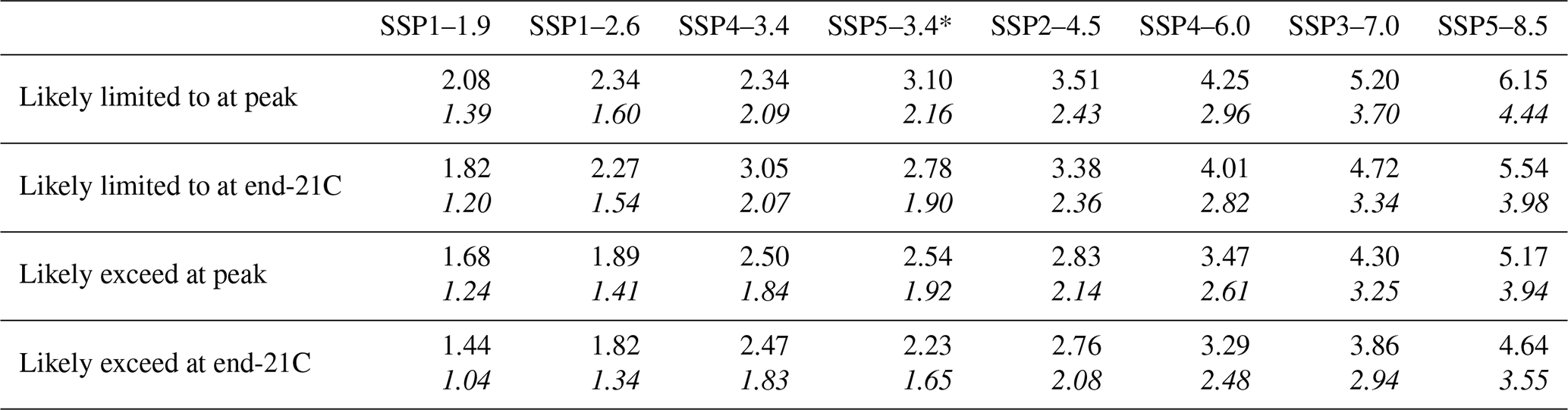
Units: ∘C. * Overshoot type pathway. Upper: Prior ensemble. Lower (in italics): Constrained ensemble
Regarding consistency with target warming levels, such as 2 ∘C above preindustrial levels, the Constrained ensemble agrees relatively well with the AR5 assessment (Collins et al., 2013) for each of the comparable Representative Concentration Pathways (RCPs; van Vuuren et al., 2011) such as RCP2.6 with SSP1–2.6. For example, AR5 states that end-21C temperature change above 2 ∘C is unlikely (0 %–33 %) under RCP2.6, which implies that temperature is likely limited to 2 ∘C. This assessment is consistent with the SSP1–2.6 result from Constrained (likely limited to 1.51 ∘C) but not from Prior (likely limited to 2.27 ∘C). Some threshold temperatures in Constrained are not consistent with AR5 such that the temperature in SSP2–4.5 likely exceeds 2.06 ∘C, while in AR5 it is more likely than not (>50 %–100 %) to exceed 2 ∘C in RCP4.5. There is a similar difference in the possibility of limiting to 4 ∘C in SSP5–8.5 and RCP8.5. AR5 assessed these cases with medium confidence rather than high confidence, implying that the reduced likely ranges (as in Constrained) can update the AR5 assessment more authentically. However, at present, the Constrained ensemble does not incorporate possible uncertainties, as discussed in the next section. It should also be noted that SSP forcing is not exactly the same as corresponding RCP forcing, leading to noticeable temperature differences between the comparable scenarios (Nicholls et al., 2020).
There are also some issues with handling of historical warming. The AR5 refers to a specific level of 0.61 ∘C from HadCRUT data for the period 1986–2005, which is added to the CMIP5 projected warming. However, HadCRUT warming is defined as an air–ocean blended temperature and is thereby somewhat underestimated for the GSAT definition (Schurer et al., 2018) with which modeled future warming is evaluated. In any case, the AR5 assessment is effectively constrained by observed warming, which may be responsible for its better agreement with the Constrained ensemble. Figure 13 indicates medians and likely (17 %–83 %) ranges of temperature changes in 2017 by the GMST (air–ocean blended) definition: 1.30 [0.96–1.81] ∘C in Prior and 0.90 [0.80–1.01] ∘C in Constrained. The latter warming levels are also closer to the SR15 assessment of 1.0 [0.8–1.2] ∘C for human-induced warming (Allen et al., 2018), despite some bias towards the lower end of the assessed range.
4.1 Performance as an emulator
It has already been confirmed that the MCE reproduces many different CMIP models effectively in terms of thermal response to idealized CO2 forcing changes, as demonstrated in Nicholls et al. (2020). The forcing and response parameters are adjusted to emulate two of the CMIP's basic experiments for step-shaped (abrupt-4xCO2) and ramp-shaped (1pctCO2) forcing increases. The forcing scheme uses different functions depending on concentration levels: a quadratic expression in terms of logarithmic concentrations in the range from 2 to 4 times the base level, smoothly connecting to linear expressions outside this range. This flexibility suits the CMIP models' tendency to deviate from logarithmic concentration proportions at higher concentrations, leading to better emulation not only for responses to quadrupling increases commonly used in basic experiments, but also for responses to considerably lower increases in many mitigation scenarios.
However, the scheme assumes constancy of the climate feedback parameter; emulation accuracy will therefore be decreased in scenarios in which state dependency of feedbacks emerges. A typical example appears in a cooling scenario. The RCMIP Phase 1 results include a case in which the MCE fails to emulate a halving CO2 experiment, while successfully emulating both doubling and quadrupling (see Fig. 2 of Nicholls et al., 2020). It is also known that state dependency becomes significant when the time integration of the step response continues over multi-centennial to millennial timescales (Knutti and Rugenstein, 2015; Rohrschneider et al., 2019). As CMIP models tend to deviate from linearity between the TOA energy imbalance and the surface temperature anomaly so that additional warming occurs with time, the MCE would result in underestimated warming in such a case. In practice, this issue is not significant up to the time horizon of 2100, which is commonly used in mitigation scenarios, in particular for lower than doubling CO2 levels.
For non-CO2 forcing, additivity is assumed across different agents, except for overlapping effects for CH4 and N2O, as parameterized in Etminan et al. (2016). The forcing amplification for CO2 is not extended to total forcing. These are reasonable assumptions for most mitigation scenarios in which non-CO2 components are presumably not extreme.
The carbon cycle module has a mixture of fixed and adjustable parameters, including those for several feedback mechanisms from temperature changes. The current configuration successfully works to represent the CMIP ESMs' ranges in terms of carbon budget in the idealized 1 %-per-year CO2 increase experiment. However, it has not yet been verified that each of the ESMs can be accurately emulated.
Diagnosing the carbon cycle parameters to individual ESMs is a main issue to be addressed in the future. Accumulated carbon in response to atmospheric CO2 input has a trade-off relationship between ocean and land, and both components have their own mechanisms of climate–carbon cycle feedbacks, which are also subject to the magnitude of temperature response. This implies that calibrating the MCE parameters for each ESM requires a series of pulse response experiments designed to allow each of the ocean and land contributions to be isolated, with and without temperature feedback. Besides the standard 1 %-per-year increase experiment, the CMIP6 provides idealized ESM experiments, including 1 %-per-year increase variants with different configurations and a variety of pathways to zero emissions (Jones et al., 2019; Keller et al., 2018). The extent to which different ESMs are emulated for these scenarios needs to be verified with calibrated parameters, leading to further insights into carbon cycle behavior in terms of amount of emissions, hysteresis effects after attaining zero emissions, and state dependency.
While the covariance of MCE parameters is incorporated for the CMIP models' variability of CO2-induced warming, the carbon cycle parameters and the non-CO2 scaling factors are independently sampled. There may be other covariance between key indicators. As different types of aerosol schemes constitute a major source of model variations, incorporating covariance associated with aerosol forcing would improve parameter sampling, leading to more appropriate indicator ranges.
The results shown in the previous section are outputs from concentration-driven experiments in which implied emissions are available for CO2 only. Likewise, the emission-driven option is currently limited to CO2. The two types of experiments are equivalent within numerical errors associated with a time integration scheme, for which Runge–Kutta fourth order is used. However, implied emissions tend to be noisy when pulse-like non-CO2 forcing is given, owing to the temperature dependency implemented in carbon cycle modules. This is the case in historical experiments including volcanic forcing.
4.2 Further improvement on constraints
The Constrained ensemble was applied to that compared in the RCMIP Phase 2 exercise, wherein the MCE is recognized as one of two models that have commonly used the target constraints, implying that they are successfully constrained, among nine participant models with different degrees of complexity (Nicholls et al., 2021). The MCE is a relatively simple emulator that is conceivably cited with a simple thermal response, an intermediate-complexity carbon cycle, simply parameterized non-CO2 GHG forcing, and no other Earth system components. This simplicity and the successful results obtained imply that a method with less complicated structures and fewer control parameters offers advantages when building reasonable parameter ensembles, despite less capacity to emulate detailed Earth system components.
Several issues require clarification with regard to the differences between Prior and Constrained ensembles. First of all, it should be emphasized that the constraints used in the RCMIP were preliminary, as the formal IPCC Sixth Assessment was not yet available during the project. Since the results from the Constrained ensemble heavily depend on recent warming trends from specific datasets without any additional uncertainties, which led to lower sensitivity indicators (Fig. 12h and i), the Constrained future warming projections and their uncertainty ranges would be underestimated compared to those based on formally assessed trends from multiple lines of evidence (IPCC, 2021).
The current proxy constraints such as the ones for the three climate sensitivity ranges of ECSG, TCR, and TCRE adopted from individual studies are not necessarily consistent with each other. The range of ECSG is based on multiple lines of evidence, including feedback process understanding, historical records, and paleoclimate records (Sherwood et al., 2020). Here, ECSG, rather than ECS, is referred to, assuming that process understanding is largely based on the CMIP's quadrupling CO2 experiments. The range of TCR is based on 30 and 22 AOGCMs from the CMIP5 and CMIP6, both constrained by warming trends during recent decades (Tokarska et al., 2020). In contrast to these observations and modeling studies, the range of TCRE is based on 11 CMIP6 ESMs (Arora et al., 2020). Improved ensembles based on comprehensively assessed constraints would increase reliability of probabilistic projections, leading to better insights into future warming.
In comparison with the AR5 assessment, the Constrained ensemble has considerably low-biased climate sensitivity, but nevertheless indicates comparable future warming across different scenarios. As stated above, this inconsistency can be partly explained on the basis of the AR5 method for warming levels that adds up observed historical warming to CMIP5-modeled future projections. With regard to consistency throughout the whole period, the emulator approach would be more desirable. In any case, it is necessary to impose appropriate weighting on CMIP models to be emulated, in particular when the model ensemble has a wide spread and some outliers in terms of reproducibility of past and current climates (Cox et al., 2018; Tokarska et al., 2020). The MH sampler with observed warming constraints corresponds to an indirect method for such weighting. As the present results decisively depend on surface temperature and OHC observations during recent decades, their validity as a constraint needs to be discussed from a broad perspective across forcing, response, and sensitivity.
The current constraining assumes observed warming as an entirely forced response. Recent findings from warming attribution studies may support this, suggesting that human-induced warming is similar to observed warming (Allen et al., 2018). However, the attribution depends on temporal and spatial patterns of forced response in multiple AOGCMs as well as their diagnosed forcing, leading to a complicated situation in which constraining data and AOGCMs to be constrained are mutually dependent. Also, substantial uncertainties of response patterns to changes in individual forcing factors remain owing to the diversity of AOGCMs (Jones et al., 2016). Moreover, the new CMIP6 models appear to have marked differences in the magnitude of internal variability underlying attribution studies (Parsons et al., 2020). The GMST constraint does not consider such uncertainties and may be replaced with broader ranges from new insights into forced response.
Furthermore, it is also necessary to constrain forced response on a centennial timescale. Besides the HadCRUT data available since 1850, the OHC data, limited to the late 20th century, may include delayed response components on a much longer timescale. In fact, major volcanic eruptions occurred frequently in the 18th and 19th centuries. The initial year of 1850 is commonly used as a proxy preindustrial time point to avoid difficulties that arise from limited observations and major eruptions (Allen et al., 2018). However, the pre-1850 volcanic impact on the deep ocean should be examined carefully. In fact, it has been recognized in historical runs with the MCE that the OHC increase during the late 20th century significantly depends on the initial year, while the surface warming does not. A series of volcanic eruptions in the period 1750–1850 appears to have contributed to heating after the period and has amplified heat content increase since 1850. The results suggest that human-induced OHC increase should be distinguished from observed total increase for better constraints.
Aerosol cooling is one of the key factors influencing temperature changes in the latter half of the 20th century, resulting in different ranges of other climate indicators. The present method relies on the prescribed ERF time series prepared for the CMIP6, which is scaled to the proxy assessment range in 2014 (Fig. 12r). Although this procedure ensures that cooling magnitude is constrained to the given range at the specific time point, the base time series is fixed. The constraint, adopted from Smith et al. (2020), is the outcome of the Radiative Forcing Model Intercomparison Project (RFMIP; Pincus et al., 2016), one of the CMIP6-endorsed model intercomparisons. Better insight into aerosol forcing may update its historical time series, thereby leading to improvement of forced response and other climate indicators, including climate sensitivity.
Technical issues exist when sampling from the Prior ensemble with observed warming constraints, associated with their distinct differences. The proxy ranges of the constraints are much more biased and localized compared to the Prior distributions, leading to inefficient sampling. The acceptance rate in the present case reached only about 1 %, requiring ∼ 105 member calibration runs to obtain a 600-member Constrained ensemble. Besides the efficiency issue, the sampling process should be visually monitored to verify whether the acceptance or rejection is reasonable. As the MH independence sampler compares a probability density ratio of the next state to the current between candidate and target densities, care is to be exercised at the distributions' tail regions where relatively large approximation errors may exist. The present method introduced ad hoc criteria to avoid acceptance with an unexpectedly large density ratio. As mentioned in Sect. 3.1 and confirmed from Fig. 12, the current method does not technically meet the MCMC requirement but still generates a reasonable ensemble that generally satisfies the RCMIP constraints. Nevertheless, methodological issues should be addressed using improved constraints.
A new climate model emulator, MCE, was developed, and its probabilistic climate projections for representative scenarios were demonstrated and thoroughly discussed. The MCE is based on impulse response functions and several parameterized physics, including key climate–carbon cycle feedbacks, and it may be categorized as a relatively low-complexity model among recent model intercomparison participants. It has an advantage when building reasonable perturbed ensembles transparently, despite its lower capacity to emulate detailed Earth system components. Perturbed ensembles can cover complex climate models' diversity effectively, reflecting their covariance structure of diagnosed forcing response parameters associated with CO2-induced warming. They can be constrained with several ranges of climate indicators, including CO2 and other forcing factors as well as observed warming trends over recent decades. The constraining procedure, implemented with a Metropolis–Hastings algorithm, effectively works as weighting given to complex models.
Results from climate assessments for future scenarios in terms of their compatibility with climate mitigation goals are preliminary, and experiments should be conducted with newly assessed constraining data. There are considerable uncertainties about forced components of historical warming as well as different forcing factors and consistency of assessed ranges among different climate sensitivity metrics. These are main issues to be clarified considering updated indicator ranges in the latest assessment. There is some room for improvement in emulator functionality. The carbon cycle module has not been configured to individual complex models, full emissions-driven experiments have not been supported, and perturbed parameter ensembles have not reflected full covariance structures of complex models. These issues are to be addressed in future work.
MCE source code and example usage scripts as used in this submission are available from the MCE GitHub repository at https://github.com/tsutsui1872/mce (last access: 18 October 2021) and archived by Zenodo (https://doi.org/10.5281/zenodo.5574895, Tsutsui, 2021).
The contact author has declared that there are no competing interests.
Publisher's note: Copernicus Publications remains neutral with regard to jurisdictional claims in published maps and institutional affiliations.
I acknowledge the steering committee and the members of RCMIP, in particular Zebedee R. J. Nicholls, for giving me the opportunity to participate in the model intercomparison. The scenario experiments with perturbed parameter ensembles in my study depend on input scenario data and constraining data provided from RCMIP.
This research has been supported by the Ministry of Education, Culture, Sports, Science and Technology (Integrated Research Program for Advancing Climate Models (TOUGOU) (grant no. JPMXD0717935457)).
This paper was edited by Julia Hargreaves and reviewed by Christopher Smith and one anonymous referee.
Allen, M. P., Dube, O., Solecki, W., Aragon-Durand, F., Cramer, W., Humphreys, S., Kainuma, M., Kala, J., Mahowald, N., Mulugetta, Y., Perez, R., Wairiu, M., and Zickfeld, K.: Framing and Context, in: Global warming of 1.5 ∘C. An IPCC Special Report on the impacts of global warming of 1.5 ∘C above pre-industrial levels and related global greenhouse gas emission pathways, in the context of strengthening the global response to the threat of climate change, sustainable development, and efforts to eradicate poverty, edited by: Masson-Delmotte, V., Zhai, P., Portner, H. O., Roberts, D., Skea, J., Shukla, P. R., Pirani, A., Moufouma-Okia, W., Pean, C., Pidcock, R., Connors, S., Matthews, J. B. R., Chen, Y., Zhou, X., Gomis, M. I., Lonnoy, E., Maycock, T., Tignor, M., and Waterfield, T., available at: https://www.ipcc.ch/sr15 (last access: 28 January 2022), 2018.
Andrews, T., Gregory, J. M., and Webb, M. J.: The dependence of radiative forcing and feedback on evolving patterns of surface temperature change in climate models, J. Climate, 28, 1630–1648, https://doi.org/10.1175/JCLI-D-14-00545.1, 2015.
Arora, V. K., Katavouta, A., Williams, R. G., Jones, C. D., Brovkin, V., Friedlingstein, P., Schwinger, J., Bopp, L., Boucher, O., Cadule, P., Chamberlain, M. A., Christian, J. R., Delire, C., Fisher, R. A., Hajima, T., Ilyina, T., Joetzjer, E., Kawamiya, M., Koven, C. D., Krasting, J. P., Law, R. M., Lawrence, D. M., Lenton, A., Lindsay, K., Pongratz, J., Raddatz, T., Séférian, R., Tachiiri, K., Tjiputra, J. F., Wiltshire, A., Wu, T., and Ziehn, T.: Carbon–concentration and carbon–climate feedbacks in CMIP6 models and their comparison to CMIP5 models, Biogeosciences, 17, 4173–4222, https://doi.org/10.5194/bg-17-4173-2020, 2020.
Clarke, L., Jiang, K., Akimoto, K., Babiker, M., Blanford, G., Fisher-Vanden, K., Hourcade, J.-C., Krey, V., Kriegler, E., Löschel, A., McCollum, D., Paltsev, S., Rose, S., Shukla, P. R., Tavoni, M., van der Zwaan, B. C. C., and van Vuuren, D. P.: Assessing transformation pathways, in: Climate Change 2014: Mitigation of Climate Change, Contribution of Working Group III to the Fifth Assessment Report of the Intergovernmental Panel on Climate Change, edited by: Edenhofer, O., Pichs-Madruga, R., Sokona, Y., Farahani, E., Kadner, S., Seyboth, K., Adler, A., Baum, I., Brunner, S., Eickemeier, P., Kriemann, B., Savolainen, J., Schlomer, S., von Stechow, C., Zwickel, T., and Minx, J. C., Cambridge University Press, Cambridge, United Kingdom and New York, NY, USA, 413–510, 2014.
Collins, M., Knutti, R., Arblaster, J., Dufresne, J.-L., Fichefet, T., Friedlingstein, P., Gao, X., Gutowski, W. J., Johns, T., Krinner, G., Shongwe, M., Tebaldi, C., Weaver, A. J., and Wehner, M.: Long-term climate change: projections, commitments and irreversibility, in: Climate Change 2013: The Physical Science Basis, edited by: Stocker, T. F., Qin, D., Plattner, G.-K., Tignor, M., Allen, S. K., Boschung, J., Nauels, A., Xia, Y., Bex, V., and Midgley, P. M., Cambridge University Press, Cambridge, United Kingdom and New York, NY, USA, 1029–1136, 2013.
Cox, P. M., Huntingford, C., and Williamson, M. S.: Emergent constraint on equilibrium climate sensitivity from global temperature variability, Nature, 553, 319–322, https://doi.org/10.1038/nature25450, 2018.
Cummins, D. P., Stephenson, D. B., and Stott, P. A.: Optimal estimation of stochastic energy balance model parameters, J. Climate, 33, 7909–7926, https://doi.org/10.1175/JCLI-D-19-0589.1, 2020.
Dickson, A. G., Sabine, C. L., and Christian, J. R. (Eds.): Guide to best practices for ocean CO2 measurements, PICES Special Publication, 3, 191 pp., 2007.
Etminan, M., Myhre, G., Highwood, E. J., and Shine, K. P.: Radiative forcing of carbon dioxide, methane, and nitrous oxide: A significant revision of the methane radiative forcing, Geophys. Res. Lett., 43, 12614–12623, https://doi.org/10.1002/2016GL071930, 2016.
Eyring, V., Bony, S., Meehl, G. A., Senior, C. A., Stevens, B., Stouffer, R. J., and Taylor, K. E.: Overview of the Coupled Model Intercomparison Project Phase 6 (CMIP6) experimental design and organization, Geosci. Model Dev., 9, 1937–1958, https://doi.org/10.5194/gmd-9-1937-2016, 2016.
Forster, P., Huppmann, D., Kriegler, E., Mundaca, L., Smith, C., Rogelj, J., and Seferian, R.: Mitigation pathways compatible with 1.5 ∘C in the context of sustainable development, Supplementary material, in: Global warming of 1.5 ∘C. An IPCC Special Report on the impacts of global warming of 1.5 ∘C above pre-industrial levels and related global greenhouse gas emission pathways, in the context of strengthening the global response to the threat of climate change, sustainable development, and efforts to eradicate poverty, edited by: Masson-Delmotte, V., Zhai, P., Portner, H. O., Roberts, D., Skea, J., Shukla, P. R., Pirani, A., Moufouma-Okia, W., Pean, C., Pidcock, R., Connors, S., Matthews, J. B. R., Chen, Y., Zhou, X., Gomis, M. I., Lonnoy, E., Maycock, T., Tignor, M., and Waterfield, T., available at: https://www.ipcc.ch/sr15 (last access: 28 January 2022), 2018.
Flynn, C. M. and Mauritsen, T.: On the climate sensitivity and historical warming evolution in recent coupled model ensembles, Atmos. Chem. Phys., 20, 7829–7842, https://doi.org/10.5194/acp-20-7829-2020, 2020.
Geoffroy, O., Saint-Martin, D., Olivié, D. J. L., Voldoire, A., Bellon, G., and Tytéca, S.: Transient climate response in a two-layer energy-balance model. Part I: Analytical solution and parameter calibration using CMIP5 AOGCM experiments, J. Climate, 26, 1841–1857, https://doi.org/10.1175/jcli-d-12-00195.1, 2013.
Goodwin, P.: Probabilistic projections of future warming and climate sensitivity trajectories, Oxford Open Climate Change, 1, kgab007, https://doi.org/10.1093/oxfclm/kgab007, 2021.
Goodwin, P. and Cael, B. B.: Bayesian estimation of Earth's climate sensitivity and transient climate response from observational warming and heat content datasets, Earth Syst. Dynam., 12, 709–723, https://doi.org/10.5194/esd-12-709-2021, 2021.
Gregory, J. M., Ingram, W. J., Palmer, M. A., Jones, G. S., Stott, P. A., Thorpe, R. B., Lowe, J. A., Johns, T. C., and Williams, K. D.: A new method for diagnosing radiative forcing and climate sensitivity, Geophys. Res. Lett., 31, L03205, https://doi.org/10.1029/2003GL018747, 2004.
Gupta, M. and Marshall, J.: The climate response to multiple volcanic eruptions mediated by ocean heat uptake: Damping processes and accumulation potential, J. Climate, 31, 8669–8687, https://doi.org/10.1175/JCLI-D-17-0703.1, 2018.
Hasselmann, K., Sausen, R., Maier-Reimer, E., and Voss, R.: On the cold start problem in transient simulations with coupled atmosphere-ocean models, Clim. Dynam., 9, 53–61, https://doi.org/10.1007/BF00210008, 1993.
Held, I. M., Winton, M., Takahashi, K., Delworth, T., Zeng, F., and Vallis, G. K.: Probing the fast and slow components of global warming by returning abruptly to preindustrial forcing, J. Climate, 23, 2418–2427, https://doi.org/10.1175/2009jcli3466.1, 2010.
Hooss, G., Voss, R., Hasselmann, K., Maier-Reimer, E., and Joos, F.: A nonlinear impulse response model of the coupled carbon cycle-climate system (NICCS), Clim. Dynam., 18, 189–202, https://doi.org/10.1007/s003820100170, 2001.
IPCC: Summary for Policymakers, in: Climate Change 2021: The Physical Science Basis. Contribution of Working Group I to the Sixth Assessment Report of the Intergovernmental Panel on Climate Change, edited by: Masson-Delmotte, V., Zhai, P., Pirani, A., Connors, S. L., Pean, C., Berger, S., Caud, N., Chen, Y., Goldfarb, L., Gomis, M. I., Huang, M., Leitzell, K., Lonnoy, E., Matthews, J. B. R., Maycock, T. K., Waterfield, T., Yelekci, O., Yu, R., and Zhou, B., Cambridge University Press, in press, https://www.ipcc.ch/report/ar6/wg1 (last access: 28 January 2022), 2021.
Jones, C. D., Frölicher, T. L., Koven, C., MacDougall, A. H., Matthews, H. D., Zickfeld, K., Rogelj, J., Tokarska, K. B., Gillett, N. P., Ilyina, T., Meinshausen, M., Mengis, N., Séférian, R., Eby, M., and Burger, F. A.: The Zero Emissions Commitment Model Intercomparison Project (ZECMIP) contribution to C4MIP: quantifying committed climate changes following zero carbon emissions, Geosci. Model Dev., 12, 4375–4385, https://doi.org/10.5194/gmd-12-4375-2019, 2019.
Jones, G. S., Stott, P. A., and Mitchell, J. F. B.: Uncertainties in the attribution of greenhouse gas warming and implications for climate prediction, J. Geophys. Res.-Atmos., 121, 6969–6992, https://doi.org/10.1002/2015JD024337, 2016.
Joos, F., Bruno, M., Fink, R., Siegenthaler, U., Stocker, T. F., Le Quéré, C., and Sarmiento, J. L.: An efficient and accurate representation of complex oceanic and biospheric models of anthropogenic carbon uptake, Tellus B, 48, 394–417, https://doi.org/10.3402/tellusb.v48i3.15921, 1996.
Keller, D. P., Lenton, A., Scott, V., Vaughan, N. E., Bauer, N., Ji, D., Jones, C. D., Kravitz, B., Muri, H., and Zickfeld, K.: The Carbon Dioxide Removal Model Intercomparison Project (CDRMIP): rationale and experimental protocol for CMIP6, Geosci. Model Dev., 11, 1133–1160, https://doi.org/10.5194/gmd-11-1133-2018, 2018.
Knutti, R. and Rugenstein, M. A. A.: Feedbacks, climate sensitivity and the limits of linear models, Philos. T. Roy. Soc. A, 373, 20150146, https://doi.org/10.1098/rsta.2015.0146, 2015.
Meehl, G. A., Moss, R., Taylor, K. E., Eyring, V., Stouffer, R. J., Bony, S., and Stevens, B.: Climate model intercomparisons: Preparing for the next phase, Eos, Trans. AGU, 95, 77–78, https://doi.org/10.1002/2014EO090001, 2014.
Meehl, G. A., Senior, C. A., Eyring, V., Flato, G., Lamarque, J.-F., Stouffer, R. J., Taylor, K. E., and Schlund, M.: Context for interpreting equilibrium climate sensitivity and transient climate response from the CMIP6 Earth system models, Sci. Adv., 6, eaba1981, https://doi.org/10.1126/sciadv.aba1981, 2020.
Meinshausen, M., Meinshausen, N., Hare, W., Raper, S. C. B., Frieler, K., Knutti, R., Frame, D. J., and Allen, M. R.: Greenhouse-gas emission targets for limiting global warming to 2 ∘C, Nature, 458, 1158–1162, https://doi.org/10.1038/nature08017, 2009.
Meinshausen, M., Raper, S. C. B., and Wigley, T. M. L.: Emulating coupled atmosphere-ocean and carbon cycle models with a simpler model, MAGICC6 – Part 1: Model description and calibration, Atmos. Chem. Phys., 11, 1417–1456, https://doi.org/10.5194/acp-11-1417-2011, 2011.
Morice, C. P., Kennedy, J. J., Rayner, N. A., and Jones, P. D.: Quantifying uncertainties in global and regional temperature change using an ensemble of observational estimates: The HadCRUT4 data set, J. Geophys. Res.-Atmos., 117, D08101, https://doi.org/10.1029/2011JD017187, 2012.
Myhre, G., Shindell, D., Bréon, F.-M., Collins, W., Fuglestvedt, J., Huang, J., Koch, D., Lamarque, J.-F., Lee, D., Mendoza, B., Nakajima, T., Robock, A., Stephens, G., Takemura, T., and Zhang, H.: Anthropogenic and natural radiative forcing, in Climate Change 2013: The Physical Science Basis, Contribution of Working Group I to the Fifth Assessment Report of the Intergovernmental Panel on Climate Change, edited by: Stocker, T. F., Qin, D., Plattner, G.-K., Tignor, M., Allen, S. K., Boschung, J., Nauels, A., Xia, Y., Bex, V., and Midgley, P. M., Cambridge University Press, Cambridge, United Kingdom and New York, NY, USA, 659–740, 2013.
Nicholls, Z. R. J., Meinshausen, M., Lewis, J., Gieseke, R., Dommenget, D., Dorheim, K., Fan, C.-S., Fuglestvedt, J. S., Gasser, T., Golüke, U., Goodwin, P., Hartin, C., Hope, A. P., Kriegler, E., Leach, N. J., Marchegiani, D., McBride, L. A., Quilcaille, Y., Rogelj, J., Salawitch, R. J., Samset, B. H., Sandstad, M., Shiklomanov, A. N., Skeie, R. B., Smith, C. J., Smith, S., Tanaka, K., Tsutsui, J., and Xie, Z.: Reduced Complexity Model Intercomparison Project Phase 1: introduction and evaluation of global-mean temperature response, Geosci. Model Dev., 13, 5175–5190, https://doi.org/10.5194/gmd-13-5175-2020, 2020.
Nicholls, Z. R. J., Meinshausen, M. A., Lewis, J., Corradi, M. R., Dorheim, K., Gasser, T., Gieseke, R., Hope, A. P., Leach, N., McBride, L. A., Quilcaille, Y., Rogelj, J., Salawitch, R. J., Samset, B. H., Sandstad, M., Shiklomanov, A. N., Skeie, R. B., Smith, C. J., Smith, S., Su, X., Tsutsui, J., Vega-Westhoff, B. A., and Woodward, D.: Reduced Complexity Model Intercomparison Project Phase 2: Synthesizing Earth system knowledge for probabilistic climate projections, Earth's Future, 9, e2020EF001900, https://doi.org/10.1029/2020EF001900, 2021.
Parsons, L. A., Brennan, M. K., Wills, R. C. J., and Proistosescu, C.: Magnitudes and spatial patterns of interdecadal temperature variability in CMIP6, Geophys. Res. Lett., 47, e2019GL086588, https://doi.org/10.1029/2019GL086588, 2020.
Pincus, R., Forster, P. M., and Stevens, B.: The Radiative Forcing Model Intercomparison Project (RFMIP): experimental protocol for CMIP6, Geosci. Model Dev., 9, 3447–3460, https://doi.org/10.5194/gmd-9-3447-2016, 2016.
Riahi, K., van Vuuren, D. P., Kriegler, E., Edmonds, J., O'Neill, B. C., Fujimori, S., Bauer, N., Calvin, K., Dellink, R., Fricko, O., Lutz, W., Popp, A., Cuaresma, J. C., Kc, S., Leimbach, M., Jiang, L., Kram, T., Rao, S., Emmerling, J., Ebi, K., Hasegawa, T., Havlik, P., Humpenöder, F., Da Silva, L. A., Smith, S., Stehfest, E., Bosetti, V., Eom, J., Gernaat, D., Masui, T., Rogelj, J., Strefler, J., Drouet, L., Krey, V., Luderer, G., Harmsen, M., Takahashi, K., Baumstark, L., Doelman, J. C., Kainuma, M., Klimont, Z., Marangoni, G., Lotze-Campen, H., Obersteiner, M., Tabeau, A., and Tavoni, M.: The Shared Socioeconomic Pathways and their energy, land use, and greenhouse gas emissions implications: An overview, Global Environ. Change, 42, 153–168, https://doi.org/10.1016/j.gloenvcha.2016.05.009, 2017.
Rogelj, J., Shindell, D., Jiang, K., Fifita, S., Forster, P., Ginzburg, V., Handa, C., Kheshgi, H., Kobayashi, S., Kriegler, E., Mundaca, L., Seferian, R., and Vilarino, M. V.: Mitigation pathways compatible with 1.5 ∘C in the context of sustainable development, in: Global warming of 1.5 ∘C. An IPCC Special Report on the impacts of global warming of 1.5 ∘C above pre-industrial levels and related global greenhouse gas emission pathways, in the context of strengthening the global response to the threat of climate change, sustainable development, and efforts to eradicate poverty, edited by: Masson-Delmotte, V., Zhai, P., Portner, H. O., Roberts, D., Skea, J., Shukla, P. R., Pirani, A., Moufouma-Okia, W., Pean, C., Pidcock, R., Connors, S., Matthews, J. B. R., Chen, Y., Zhou, X., Gomis, M. I., Lonnoy, E., Maycock, T., Tignor, M., and Waterfield, T., available at: https://www.ipcc.ch/sr15 (last access: 28 January 2022), 2018.
Rohrschneider, T., Stevens, B., and Mauritsen, T.: On simple representations of the climate response to external radiative forcing, Clim. Dynam., 53, 3131–3145, https://doi.org/10.1007/s00382-019-04686-4, 2019.
Schurer, A. P., Cowtan, K., Hawkins, E., Mann, M. E., Scott, V., and Tett, S. F. B.: Interpretations of the Paris climate target, Nat. Geosci., 11, 220–221, https://doi.org/10.1038/s41561-018-0086-8, 2018.
Schwarber, A. K., Smith, S. J., Hartin, C. A., Vega-Westhoff, B. A., and Sriver, R.: Evaluating climate emulation: fundamental impulse testing of simple climate models, Earth Syst. Dynam., 10, 729–739, https://doi.org/10.5194/esd-10-729-2019, 2019.
Sherwood, S. C., Bony, S., Boucher, O., Bretherton, C., Forster, P. M., Gregory, J. M., and Stevens, B.: Adjustments in the forcing-feedback framework for understanding climate change, B. Am. Meteorol. Soc., 96, 217–228, https://doi.org/10.1175/BAMS-D-13-00167.1, 2015.
Sherwood, S., Webb, M. J., Annan, J. D., Armour, K. C., Forster, P. M., Hargreaves, J. C., Hegerl, G., Klein, S. A., Marvel, K. D., Rohling, E. J., Watanabe, M., Andrews, T., Braconnot, P., Bretherton, C. S., Foster, G. L., Hausfather, Z., Heydt, A. S. von der, Knutti, R., Mauritsen, T., Norris, J. R., Proistosescu, C., Rugenstein, M., Schmidt, G. A., Tokarska, K. B., and Zelinka, M. D.: An assessment of Earth’s climate sensitivity using multiple lines of evidence, Rev. Geophys., e2019RG000678, https://doi.org/10.1029/2019RG000678, 2020.
Smith, C. J. and Forster, P. M.: Suppressed late-20th Century warming in CMIP6 models explained by forcing and feedbacks, Geophys. Res. Lett., e2021GL094948, https://doi.org/10.1029/2021GL094948, 2021.
Smith, C. J., Forster, P. M., Allen, M., Leach, N., Millar, R. J., Passerello, G. A., and Regayre, L. A.: FAIR v1.3: a simple emissions-based impulse response and carbon cycle model, Geosci. Model Dev., 11, 2273–2297, https://doi.org/10.5194/gmd-11-2273-2018, 2018.
Smith, C. J., Kramer, R. J., Myhre, G., Alterskjær, K., Collins, W., Sima, A., Boucher, O., Dufresne, J.-L., Nabat, P., Michou, M., Yukimoto, S., Cole, J., Paynter, D., Shiogama, H., O'Connor, F. M., Robertson, E., Wiltshire, A., Andrews, T., Hannay, C., Miller, R., Nazarenko, L., Kirkevåg, A., Olivié, D., Fiedler, S., Lewinschal, A., Mackallah, C., Dix, M., Pincus, R., and Forster, P. M.: Effective radiative forcing and adjustments in CMIP6 models, Atmos. Chem. Phys., 20, 9591–9618, https://doi.org/10.5194/acp-20-9591-2020, 2020.
Smith, C. J., Harris, G. R., Palmer, M. D., Bellouin, N., Collins, W., Myhre, G., Schulz, M., Golaz, J.-C., Ringer, M., Storelvmo, T., and Forster, P. M.: Energy budget constraints on the time history of aerosol forcing and climate sensitivity, J. Geophys. Res.-Atmos., 126, e2020JD033622, https://doi.org/10.1029/2020JD033622, 2021.
Tanaka, K., Kriegler, E., Bruckner, T., Hooss, G., Knorr, W., Raddatz, T., and Tol, R.: Aggregated Carbon Cycle, Atmospheric Chemistry, and Climate Model (ACC2): Description of the forward and inverse modes, Max-Planck-Institut für Meteorologie, available at: https://pure.mpg.de/rest/items/item_994422/component/file_994421/content (last access: 28 January 2022), 2007.
Taylor, K. E., Stouffer, R. J., and Meehl, G. A.: An overview of CMIP5 and the experiment design, B. Am. Meteorol. Soc., 93, 485–498, https://doi.org/10.1175/bams-d-11-00094.1, 2012.
Tokarska, K. B., Stolpe, M. B., Sippel, S., Fischer, E. M., Smith, C. J., Lehner, F., and Knutti, R.: Past warming trend constrains future warming in CMIP6 models, Sci. Adv., 6, eaaz9549, https://doi.org/10.1126/sciadv.aaz9549, 2020.
Tsutsui, J.: Quantification of temperature response to CO2 forcing in atmosphere–ocean general circulation models, Clim. Change, 140, 287–305, https://doi.org/10.1007/s10584-016-1832-9, 2017.
Tsutsui, J.: Diagnosing transient response to CO2 forcing in coupled atmosphere-ocean model experiments using a climate model emulator, Geophys. Res. Lett., 47, e2019GL085844, https://doi.org/10.1029/2019GL085844, 2020.
Tsutsui, J.: Minimal CMIP Emulator (MCE v1.2.1), Zenodo [code], https://doi.org/10.5281/zenodo.5574895, 2021.
van Vuuren, D. P., Edmonds, J., Kainuma, M., Riahi, K., Thomson, A., Hibbard, K., Hurtt, G. C., Kram, T., Krey, V., Lamarque, J.-F., Masui, T., Meinshausen, M., Nakicenovic, N., Smith, S. J., and Rose, S. K.: The representative concentration pathways: an overview, Clim. Change, 109, 5, https://doi.org/10.1007/s10584-011-0148-z, 2011.
von Schuckmann, K., Cheng, L., Palmer, M. D., Tassone, C., Aich, V., Adusumilli, S., Beltrami, H., Boyer, T., Cuesta-Valero, F. J., Desbruyères, D., Domingues, C., García-García, A., Gentine, P., Gilson, J., Gorfer, M., Haimberger, L., Ishii, M., Johnson, G. C., Killick, R., King, B. A., Kirchengast, G., Kolodziejczyk, N., Lyman, J., Marzeion, B., Mayer, M., Monier, M., Monselesan, Didier Paolo, Purkey, S., Roemmich, D., Schweiger, A., Seneviratne, S. I., Shepherd, A., Slater, D. A., Steiner, A. K., Straneo, F., Timmermanns, M.-L., and Wijffels, S. E.: Heat stored in the Earth system: Where does the energy go?, WDC Climate, https://doi.org/10.26050/WDCC/GCOS_EHI_EXP, 2020.
Zelinka, M. D., Myers, T. A., McCoy, D. T., Po-Chedley, S., Caldwell, P. M., Ceppi, P., Klein, S. A., and Taylor, K. E.: Causes of higher climate sensitivity in CMIP6 models, Geophys. Res. Lett., 47, e2019GL085782, https://doi.org/10.1029/2019GL085782, 2020.