the Creative Commons Attribution 4.0 License.
the Creative Commons Attribution 4.0 License.
 | 23 Dec 2022
UniFHy v0.1.1: a community modelling framework for the terrestrial water cycle in Python
Thibault Hallouin
Richard J. Ellis
Douglas B. Clark
Simon J. Dadson
Andrew G. Hughes
Bryan N. Lawrence
Grenville M. S. Lister
Jan Polcher
The land surface, hydrological, and groundwater modelling communities all have expertise in simulating the hydrological processes at play in the terrestrial component of the Earth system. However, these communities, and the wider Earth system modelling community, have largely remained distinct with limited collaboration between disciplines, hindering progress in the representation of hydrological processes in the land component of Earth system models (ESMs). In order to address key societal questions regarding the future availability of water resources and the intensity of extreme events such as floods and droughts in a changing climate, these communities must come together and build on the strengths of one another to produce next-generation land system models that are able to adequately simulate the terrestrial water cycle under change. The development of a common modelling infrastructure can contribute to stimulating cross-fertilisation by structuring and standardising the interactions. This paper presents such an infrastructure, a land system framework, which targets an intermediate level of complexity and constrains interfaces between components (and communities) and, in doing so, aims to facilitate an easier pipeline between the development of (sub-)community models and their integration, both for standalone use and for use in ESMs. This paper first outlines the conceptual design and technical capabilities of the framework; thereafter, its usage and useful characteristics are demonstrated through case studies. The main innovations presented here are (1) the interfacing constraints themselves; (2) the implementation in Python (the Unified Framework for Hydrology, unifhy); and (3) the demonstration of standalone use cases using the framework. The existing framework does not yet meet all our goals, in particular, of directly supporting integration into larger ESMs, so we conclude with the remaining limitations of the current framework and necessary future developments.
- Article
(5856 KB) - Full-text XML
-
Supplement
(299 KB) - BibTeX
- EndNote


The Earth’s atmosphere and land surface are highly interconnected systems with significant interactions and feedback (Betts et al., 1996). Given this, hydrological knowledge is as critical to atmospheric scientists as meteorological knowledge is to hydrologists. These interactions have long been represented in land surface models (LSMs) (Blyth et al., 2021). However, they were historically developed as a lower boundary condition, and they remain intimately connected to atmospheric models to this day. This partially explains the remaining shortcomings in the representation of hydrological processes in LSMs. In particular, the resolution of the land system coupled with the atmosphere has typically been too coarse to adequately represent the spatial structures of the dominant hydrological processes (Fisher and Koven, 2020), while the focus on vertical exchanges between the land and the atmosphere has limited the development of the critical lateral redistribution of water on and below the ground (Clark et al., 2015a). To overcome these limitations, a modular representation of the terrestrial water cycle using interconnected modelling components would provide the flexibility required in the spatial discretisation of the land system while preserving the existing coupling approaches with atmospheric models. In turn, such modularity would facilitate the contributions from distinct modelling communities with expertise in the terrestrial water cycle, that are the land surface, hydrological, and groundwater modellers, as long as the interfaces between the modular elements are clearly specified. In particular, introducing this modularity would allow the testing of models of varying complexity to determine its impact on simulations. However, such modular framework does not exist yet for LSMs, despite a variety of existing frameworks developed within the distinct communities with expertise in simulating the terrestrial water cycle.
The land surface modelling community has developed highly configurable models such as the Joint UK Land Environment Simulator (JULES) (Best et al., 2011; Clark et al., 2011), the Organising Carbon and Hydrology In Dynamic Ecosystems (ORCHIDEE) model (Krinner et al., 2005), and the Community Land Model (CLM) (Lawrence et al., 2019). However, these models do not allow different parts of the land system to be simulated at different explicit resolutions (except for the runoff routing), nor do they make it possible to substitute part of one model with another part from a different model, which are crucial requirements to advance land surface modelling (Blyth et al., 2021).
The Earth surface dynamics modelling community has developed coupling frameworks for the land system, e.g. Landlab (Hobley et al., 2017; Barnhart et al., 2020) can be used to develop modelling components complying with the Basic Model Interface (BMI) (Peckham et al., 2013; Hutton et al., 2020) that can be coupled using the Python Modelling Toolkit (PyMT) (Hutton et al., 2021). However, these frameworks are primarily developed to address requirements of geomorphologists. Therefore, they do not consider the essential need for LSMs to be coupled with external models, e.g. atmospheric models, where the handling of time advancement and memory allocation of the land model need to be delegated to an external model.
The hydrological modelling community has also been developing frameworks of varying granularity to compare different physical processes and/or conceptualisations of the hydrological behaviour of a hydrological system. For example, FUSE (Clark et al., 2008) and SUPERFLEX (Fenicia et al., 2011) provide bucket-style building blocks to develop integrated catchment models, while CMF (Kraft et al., 2011), SUMMA (Clark et al., 2015b), and Raven (Craig et al., 2020) allow the construction of physically explicit hydrological models by providing finer building blocks in the form of the process equation themselves. However, given the large number of processes included in LSMs, our experience reveals that refactoring existing models using these frameworks is not trivial, and an intermediate level of granularity is required to simplify their refactoring. The Open Modelling Interface (OpenMI) has been developed to provide an international standard to link hydrological and hydraulic models as components. It has been implemented as a flexible approach for allowing models as components to be linked at runtime (Harpham et al., 2019). However, despite its flexibility, there is no standardised interface for linking OpenMI compliant components which reduces their compatibility and continued reusability over time.
The Earth system modelling community has also developed frameworks with intermediate modularity, where atmosphere, ocean, and land components together simulate the dynamics of the Earth system. The technologies used to combine such modelling components range from integrated coupling frameworks such as ESMF (Collins et al., 2005) or CPL7 (Craig et al., 2012), where existing modelling components require code refactoring to comply with a set of organising and interfacing requirements, to couplers such as OASIS-MCT (Valcke, 2013; Craig et al., 2017), or YAC (Hanke et al., 2016), where existing modelling components require minimal additions to expose their variables to the coupler. While these two families of frameworks vary in the level of intrusiveness into the existing code, they both offer access to essential functionalities such as I/O, parallelism, flexible spatial discretisation, remapping, and so on. In addition, the community has developed standardised interfaces between the components (see e.g. Polcher et al., 1998; Best et al., 2004). While this experience and these technologies ought to be exploited to build modular land system models, these frameworks do not consider the specific challenges in the land system and the hydrological cycle. In particular, linear interpolation which is applicable in the remapping in continua such as those of the atmosphere and of the ocean is problematic for the land continuum because of strong discontinuities on and below the ground. In addition, the spatial discretisations typically used in Earth system modelling frameworks lack meaning for the hydrological cycle. This is why a modular framework specific to the land system is required.
The increasing complexity of LSMs renders the monolithic structure they have today untenable for future development. However, the LSM community contributing to Earth system models (ESMs) cannot adopt the coupling frameworks of the Earth surface dynamics community since they are not compatible with the complexity, parallelisation, and optimisation needs of ESMs, nor can it adopt highly modular hydrological modelling frameworks because their granularity is too fine for practical implementations with LSMs. An intermediate approach is thus needed for land system models where subcomponents of the land system are defined with clear interfaces which can be implemented with current ESM couplers. This should introduce a granularity within LSMs similar to the one of current ESMs with only a few components (i.e. atmosphere, ocean, land, cryosphere, etc.).
In this paper, a standardised subdivision of the water cycle in the land system is introduced, and a framework implementing it is described. It follows an integrated coupling philosophy featuring three framework components interconnected through standardised interfaces. The current state of development does not yet meet all goals to be embedded in ESMs, but there is enough functionality for standalone use cases. The remainder of the paper is structured as follows: Sect. 2 expands on its design principles and implementation details, Sect. 3 showcases usage of the framework, Sect. 4 details how to contribute to the framework with new science components, Sect. 5 demonstrates the capabilities of the existing framework on case studies, and finally Sect. 6 provides some conclusions including the development directions which will be necessary to meet the goals of integration in Earth system models.
2.1 Modular water cycle blueprint
Given the dominant spatial structures and temporal scales of the processes involved in the terrestrial water cycle, and the interconnected nature of the land system with the atmosphere and the ocean, a modular blueprint featuring three framework components is chosen (see Fig. 1): a surface layer component encapsulating the dynamics of moisture and energy exchanges between the atmosphere and the Earth's surface, which are amongst the fastest processes in the terrestrial water cycle and predominantly unidirectional (i.e. vertical); a subsurface component to address the movement of water through the soil down to the bedrock, which in comparison tends to be slower and truly tridirectional (i.e. lateral redistribution according to topographic and hydraulic head gradients, and vertical percolation/capillary rise/vegetation uptake); and an open water component for the movement of free water in contact with the atmosphere which is of intermediate speed and predominantly bidirectional along the surface of the Earth towards the seas and oceans. Despite this modularity, each component must be conservative with respect to the quantities in the continuity equations so that these are also conserved across the entire land system.
For existing modelling components to be coupled, outputs from one need to be mapped onto inputs for another: this requires a common bank of defined variables, i.e. an ontology, to guarantee that the output of one is semantically equivalent to the input of the other. Moreover, to maximise the chances of finding compatible models, this calls for a common interface between components that skilfully yet pragmatically subdivides the terrestrial water cycle continuum. Indeed, a compromise must be found between allowing flexibility in model construction and maximising the potential for existing models to be incorporated in the framework. This is why the degrees of freedom offered to the user are intentionally limited and a standard interface between the components of the framework is formulated. This interface is a set of prescribed transfers of information between each pair of components in the blueprint. For instance, the open water component is receiving (i.e. inward transfers) “direct throughfall flux”, “water evaporation flux from open water”, “surface runoff flux delivered to rivers”, and “net subsurface flux to rivers”, while it is sending (i.e. outward transfers) “open water area fraction” and “open water surface height” (see Fig. 1 and Table 1). These interfaces define the relationship between the framework components. They were designed considering the existing structure of land surface models, namely JULES (Best et al., 2011; Clark et al., 2011) and ORCHIDEE (Krinner et al., 2005), and are the fruit of considerable consultation. The information transferred through the interface includes the fluxes necessary to fulfil the continuity equations across the entire land system, as well as the diagnostic quantities characterising the state of components which necessarily condition fluxes in other components.

Figure 1Schematic blueprint of the terrestrial water cycle featuring the three components “Surface Layer”, “Sub-Surface”, and “Open Water”, their transfers of information as numbered arrows (see Table 1), and their relationships with external models (atmosphere and ocean).
Table 1Prescribed interface variables defining what must be transferred between the framework components.

∗ Standing and open water both refer to the water on the land surface in direct contact with the atmosphere, but the former corresponds to the ephemeral water on the land surface, while the latter corresponds to the water in rivers and lakes. Total water refers to the combination of standing and open water, taking into account any overlap between the two.
2.2 Integrated coupling approach
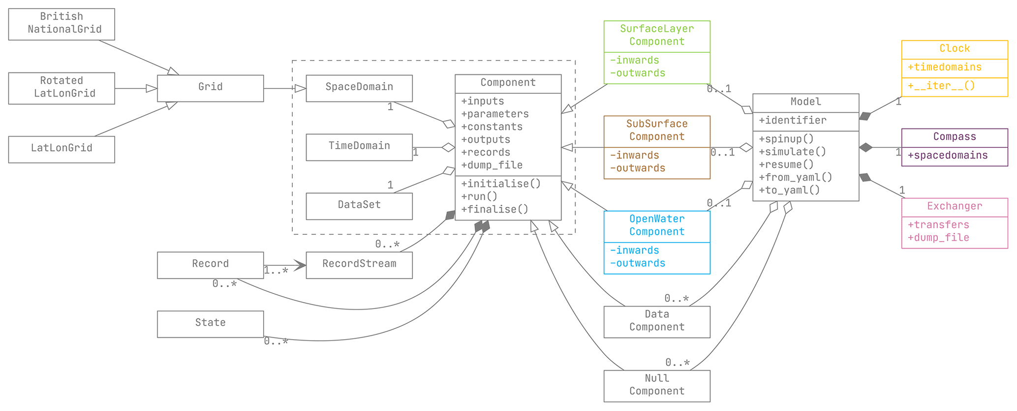
A first implementation of this blueprint is developed in Python (Hallouin and Ellis, 2021) as an integrated coupling framework following an object-oriented approach (see Fig. 2 for a visual overview of the software architecture using the Unified Modelling Language (UML)). Object-oriented programming is ideally suited to efficiently implement such modular software: the inheritance of the core functionalities of a framework component allows for code reuse in the constitution of the various subdivisions of the water cycle, and ultimately the development of community-based component contributions.
In this framework, three Component objects are coupled together by a Model object and executed concurrently, so that the order in which the components are called does not have an impact on the outcome of the simulation. The Model is responsible for the exchange of information between components, including their potential temporal accumulation and aggregation and/or their potential spatial remapping (using an Exchanger object), and is responsible for the time advancement of all components (using a Clock object).
The Component object provides infrastructure to support the science component; e.g. reading input (using DataSet objects), writing output (using Record and RecordStream objects), and state memory allocation (using State objects). The Component class itself is subclassed into the actual framework components represented by the SurfaceLayerComponent, SubSurfaceComponent, and OpenWaterComponent classes, which are used to enforce inward and outward transfers corresponding to the framework interfaces. Each accommodates the description of the physical processes of a given part of the terrestrial water cycle (i.e. the science component) following an initialise-run-finalise (IRF) paradigm. The DataComponent and NullComponent classes are also provided as a convenience to allow any of the three framework components to be either replaced with appropriate data or removed. In both cases, the replacement generates outward data transfers: in the former case, from data, in the latter case, zeros. Attempted inward data transfers are quietly ignored.
2.3 Flexible discretisation
The framework modularity makes it possible to resolve the processes in each science component at their own temporal and spatial resolutions. Each Component is discretised individually with its own instances of the TimeDomain and SpaceDomain classes defining their temporal and spatial discretisations, respectively.
In the framework, the TimeDomain class limits instances to temporal discretisations that are regularly spaced. While each component could theoretically run on any temporal resolution independent of the resolution of the other components, it is essential to make sure that restarting times exist across the simulation period in case there are unexpected interruptions of the execution. In order to achieve this, the Clock object makes sure that the temporal resolutions are constrained such that, across the three components, the component temporal resolutions are required to be integer multiples of each other and the component temporal extents to span the same simulation period. These temporal discretisations act as a contract signed between the components and the framework to guarantee that the latter can orchestrate the simulation, but this does not need to preclude components from employing sub-time steps or adaptive time-stepping schemes internally.
In the framework, the SpaceDomain class is subclassed into a Grid, intended to encompass all structured gridded spatial discretisation. The distinction between SpaceDomain and Grid is done in anticipation of additional subclasses to be created in the future (e.g. unstructured grids). The Grid class itself currently features three subclasses corresponding to two discretisations on spherical coordinate systems (latitude–longitude and rotated-pole latitude–longitude) as well as one discretisation on a Cartesian (projected) coordinate system (the British national grid), but additional subclasses can easily be developed. Internal spatial remapping between differing component discretisations relies on the remapping functionality provided by ESMF (Collins et al., 2005). If components are to be resolved on different spatial discretisations, not only must the components conserve the quantities in the continuity equations, but the remapping operation must also be conservative. With discontinuities being intrinsic to the land system, e.g. in land cover or soil properties, it appears unrealistic to directly apply traditional interpolation methods for the remapping since they assume continuity, whereas supermeshing techniques (Farrell et al., 2009), where a supermesh is the union of the components meshes, offer solutions to remain conservative in the remapping without the need for a continuity assumption. Since the current implementation of the framework does not yet feature an explicit supermeshing technique across the three components, the Compass object makes sure that components are discretised using space domains of the same class (i.e. in the same coordinate system), that they span the same region, and that their spatial resolutions are encapsulated in one another, which effectively guarantees that for each pair of coupled components, one is the supermesh for both of them.
2.4 Open science library
Alongside the framework infrastructure itself, an initial library of open source science components complying with the standard framework interface is available. This allows users to explore alternative combinations of components as alternative solutions to simulate the terrestrial water cycle.
Additional components can be exploited by the framework as long as they comply, or can be made to comply, with the framework interface via a particular Python class template (see Listing 8).
Land system and hydrological modellers are encouraged to become contributors to the framework by sharing their science components with the rest of the community. These contributions can be implemented purely in Python, but can also rely on Fortran, C, or C++ programs called by interface middleware. Contributors need not handle basic functionalities such as memory allocation nor input/output operations, as these are handled by the framework. Ideally, the use of the framework will simplify model development allowing framework contributors to focus on scientific development (see Sect. 4).
2.5 Meaningful data
The interface specification is effectively a data specification. To guarantee the unambiguous specification of that interface, as well as bringing a full awareness of the physical meaning and spatio-temporal context of input and output data to the framework and to users alike, the NetCDF Climate and Forecast (CF) Metadata Conventions (Eaton et al., 2020) are exploited in the framework. These conventions provide a robust guide for describing, processing, and sharing geophysical data files. They are used in a variety of applications, including for global model intercomparison efforts such as CMIPs (e.g. Eyring et al., 2016). In particular, the list of CF standard names provides the main ontology followed for the naming of the fields in the framework interfaces, although given that it does not include some concepts relevant specifically for hydrology, some digression from this ontology exists in the framework until these concepts are submitted for inclusion in the list of CF standard names.
The DataSet class responsible for providing each Component with input data relies on reading CF–NetCDF files. This enables the framework to check the compatibility between the data and the configured component, both physically and spatio-temporally. In addition, all record files and dump files are generated as CF–NetCDF files. Such CF–NetCDF files are processed with the package cf-python (Hassell et al., 2017; Hassell and Bartholomew, 2020).
This section describes a typical step-by-step user workflow through an example setup. The workflow can be subdivided into a configuration stage and a simulation stage as illustrated in Fig. 3. Each stage is described step by step in the two following subsections.
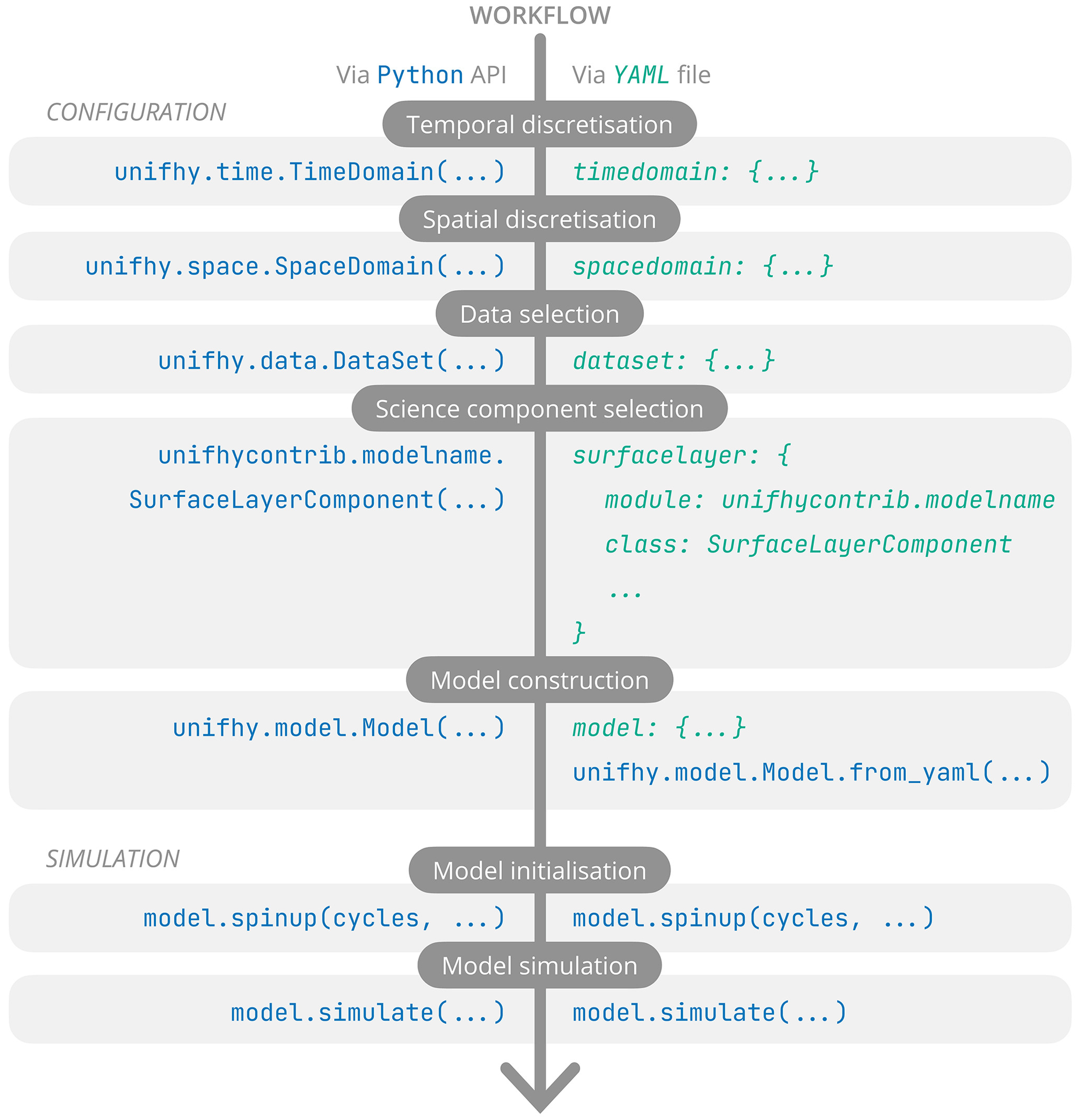
Figure 3Workflow to follow to configure and use the modelling framework, exclusively via the Python API on the left-hand side, and via the use of a YAML file for configuration on the right-hand side.
3.1 Configuration
In this subsection, the framework configuration workflow is presented. The user can configure the framework by using either the Application Programming Interface (API) directly or an intermediate YAML (Yet Another Markup Language) configuration file (summarised on the right-hand side and on the left-hand side of Fig. 3, respectively). These two configuration alternatives are presented in turn below.
3.1.1 Application programming interface
The first step in this workflow is to define the temporal and spatial discretisations. The user has to instantiate TimeDomain and SpaceDomain objects. The framework comes with a variety of constructor methods for these two objects, including using existing CF-compliant data structures, e.g. from_field, or using the limits and spacing of the discretisation, e.g. from_start_end_step for TimeDomain and from_extent_and_resolution for SpaceDomain. Examples using the latter are presented in Listing 1.
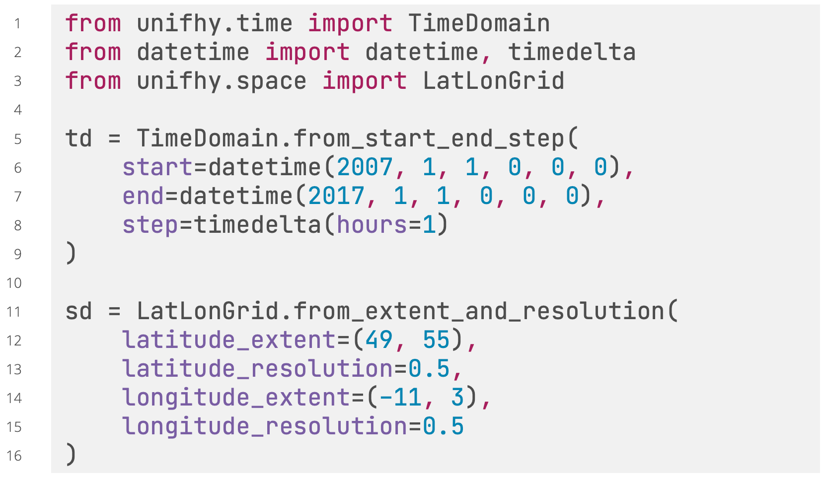
Listing 1Python script showing an example of temporal discretisation (to generate hourly timestepping), and spatial discretisation (to generate a regular 0.5∘ latitude–longitude grid) using the framework's API.
The second step consists of selecting the NetCDF files containing the input data. To do so, the user has to instantiate a DataSet object (Listing 2). These files must comply with the CF-conventions (Sect. 2.5).
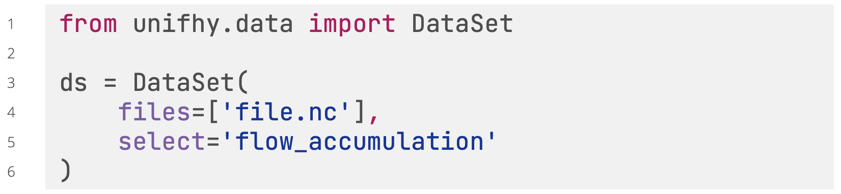
Listing 2Python script showing an example of data specification using the framework's API: selecting the “flow accumulation” variable from a CF–NetCDF file.
The third step, which completes the configuration of a Component, is to select a science component and to provide these three objects to it alongside values with units for the component parameters and constants (e.g. lines 3–15 in Listing 3). Additionally, the user can select the variables to record for this component, whether component outward transfers and/or component outputs and/or component states with customisable temporal resolutions (multiples of its TimeDomain resolution) and summary statistics (mean, minimum, maximum, instantaneous) (e.g. lines 16–18 in Listing 3). For example, in Listing 3, the open water science component RFM, based on the River Flow Model (Bell et al., 2007; Dadson et al., 2011), is used and configured (note that the science components do not come with the framework and need to be installed separately). Instantiating a Component will only be successful if all the inputs, parameters, and constants required by the science component are provided and compatible in names, units, temporal and spatial dimensions with the component and its time and space domains.
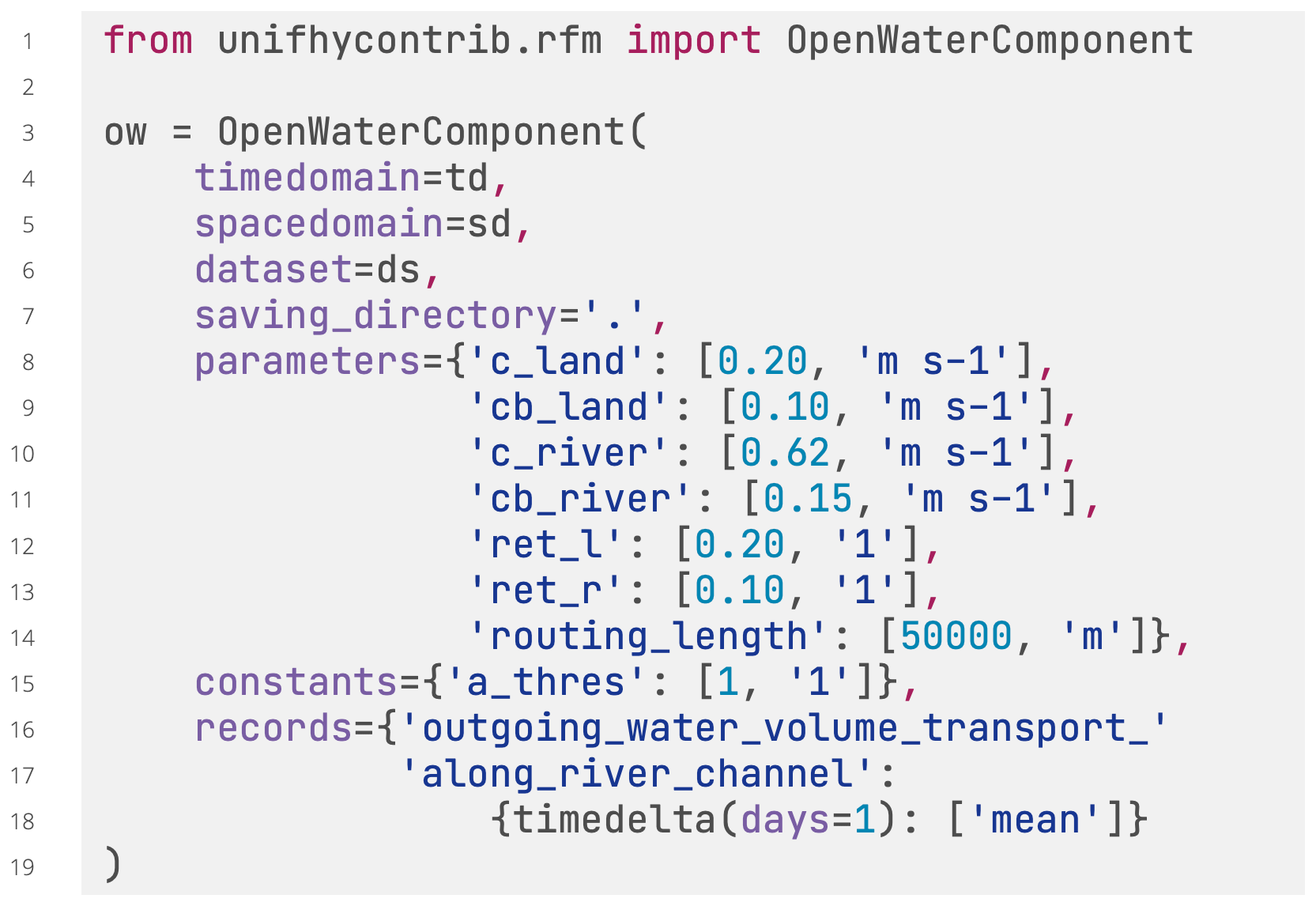
Listing 3Python script showing an example of component configuration using the framework's API: an open water component based on the RFM model is chosen; it is given the temporal and spatial discretisation instantiated before, as well as seven parameter values and one constant value; it is also requested to record one mean daily output.
The fourth and last step in the configuration workflow is to gather three components, one of each of the three types SurfaceLayerComponent, SubSurfaceComponent, and OpenWaterComponent to form a model. For example, in Listing 4, the variables “sl”, “ss”, and “ow” are instances of each, respectively, configured similarly to the example in Listing 3.
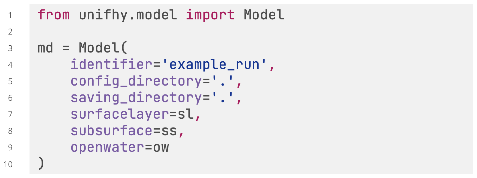
Listing 4Python script showing an example of model configuration using the framework's API: a model is instantiated by combining three components previously configured (i.e. sl, ss, and ow); by giving it a unique identifier, and by specifying paths to configuration and saving directories.
Note, the three components forming the model need to comply with the temporal and spatial discretisation constraints formulated in Sect. 2.3 for the instantiation of a Model to be successful.
3.1.2 Configuration file
An alternative to the API is the use of a configuration file written using the human-readable serialisation language YAML. This provides a more accessible configuration approach for users less comfortable with programming and a way to easily share configurations with other users. The complete configuration workflow presented above using the API can be formulated in a single YAML file. For reasons of brevity, only an equivalent for the third step above, i.e. configuring one component (Listing 3), is presented in Listing 5. Entire configuration files can be found in the Supplement.

Listing 5Excerpt from YAML configuration file semantically strictly equivalent to Listing 3.
Configuration files can then be loaded using the API to instantiate the Model directly (Listing 6). Note that after the successful instantiation of a Model using the API (i.e. Listing 4), such a YAML file is automatically created in the configuration directory.
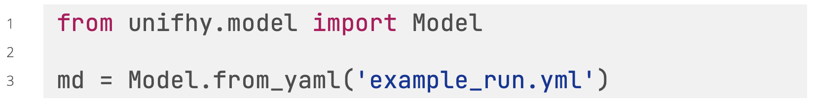
Listing 6Python script showing an example using the framework's API to instantiate a Model from a YAML configuration file.
3.2 Simulation
A configured Model can then be used to start model spin-up cycle(s) and/or to start a simulation run over the entire simulation period specified in the time domains of the components (Listing 7). The spin-up period can either be within or outside of the simulation period, as long as the datasets given to the components contain data for it.
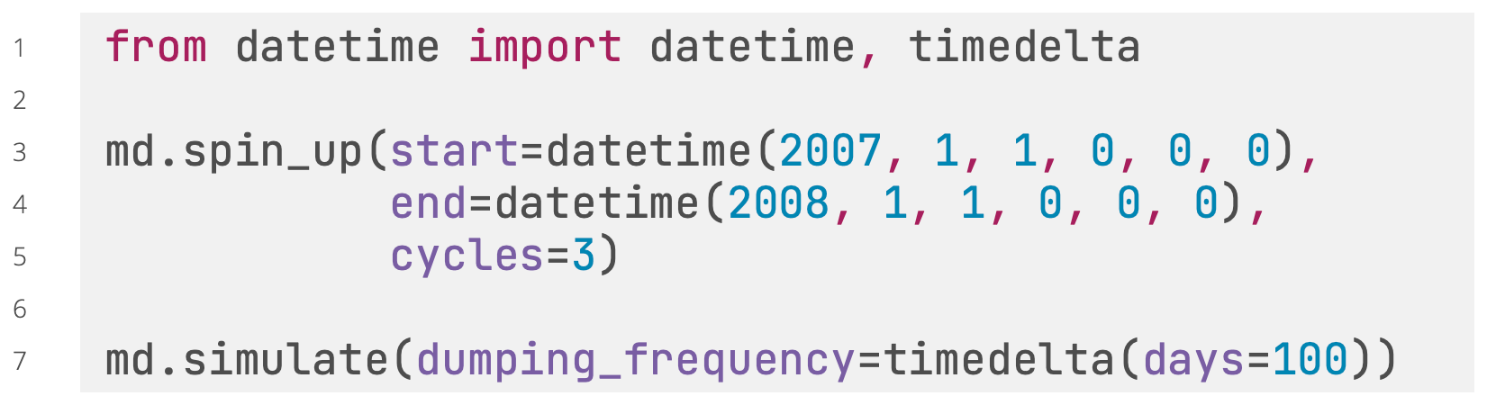
Listing 7Python script showing an example using the framework's API to start simulations with a Model.
Both spin-up and simulation runs can produce dump files, i.e. files containing intermediate snapshots in the simulation period with all the information required to resume the simulation in case of an unexpected interruption. The user can specify a dumping frequency to choose how often such snapshots should be saved. Once the Model is re-instantiated using its configuration file created through Listing 4, the simulation can be resumed using any snapshot in these dump files. Moreover, these files can be used to provide initial conditions for the component states in replacement or in addition to the spin-up cycles.
Note that detailed documentation is available online and accessible at https://unifhy-org.github.io/unifhy (last access: 20 December 2022).
If the science components already available in the open science library (Sect. 2.4) are not sufficient or suitable for the needs of users, they have the opportunity to create their own. New science components for use in the framework must be developed as Python subclasses of the framework's internal SurfaceLayerComponent, SubSurfaceComponent, and OpenWaterComponent classes.
The approach to developing a science component is designed to require minimal development effort, and can be divided into five steps. The first step is to declare a Python class whose base class is one of the SurfaceLayerComponent, SubSurfaceComponent, or OpenWaterComponent classes (e.g. lines 1–4 in Listing 8). The second step is to provide a description for the component using the docstring of the class (e.g. line 5 in Listing 8). The third step is to declare the component interface, i.e. to indicate which transfers in the standard interface are used and produced (e.g. lines 8–9 in Listing 8). The fourth step is to define the component characteristics, including its inputs, parameters, constants, states, and outputs in their corresponding class attributes (e.g. lines 10–26 in Listing 8). The fifth and last step is to implement the three class methods initialise, run, and finalise (e.g. lines 29–42 in Listing 8, where the pass statements should be replaced by the actual implementation of these methods). This initialise-run-finalise (IRF) paradigm is based on the interfacing standards BMI (Peckham et al., 2013; Hutton et al., 2020) and OpenMI (Harpham et al., 2019).
Thanks to their base classes, they inherit the functionality that make them readily usable in the framework, as described in Sect. 3, such that instances of newly created Component classes can then be directly created (following the same approach as in Listing 4).
It is possible that, for existing models, the contributor may need to perform some refactoring of their source code, namely to comply with the framework interfaces and to comply with the IRF paradigm. While the creation of a Python class is a requirement for use in the framework, the initialise, run, and finalise methods can call software which can be interfaced with Python, such as existing Fortran, C, or C++ programs. Contributors interested in interfacing C/C++ or Fortran methods are invited to take a look at the components used in the unit tests of the framework to get started.
Note that on a scientific level, there is no a priori restriction on the degree of complexity that models must meet to be refactored into science components, only their compatibility with the framework's standardised interface is expected. Nonetheless, Blyth et al. (2021) provides a good overview of the class of models primarily targeted.
A blank template is available on GitHub at https://github.com/unifhy-org/unifhycontrib-template (last access: 20 December 2022) to provide a starting point for contributors to package their new or existing models into framework-compatible Python libraries, and contributors are invited to follow the step-by-step description on component contributions available in the online documentation.
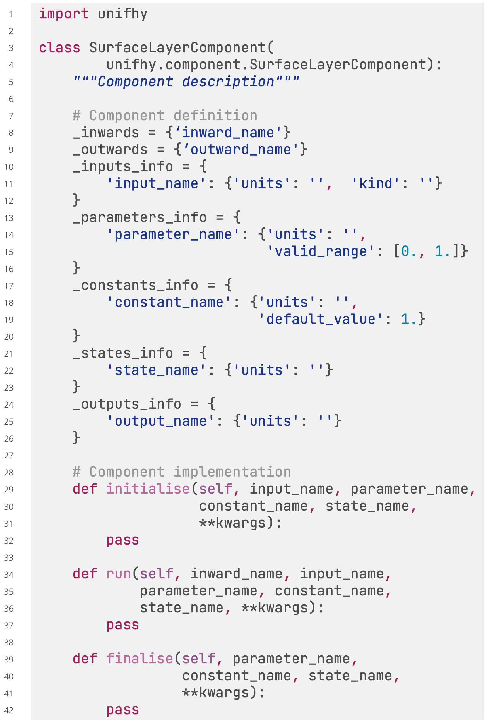
Listing 8Python script showcasing the template to follow to develop a new science component contribution presented through an example with a fictional surface layer component whose definition and implementation are kept intentionally generic and trivial, respectively.
This section introduces case studies as demonstration and illustration material of the capabilities of the framework detailed above, i.e. allowing users to choose and configure various modelling components to simulate the terrestrial water cycle. The selected science components, their configurations in the framework, and the study catchments are presented before some outputs obtained with the framework are briefly presented and evaluated.
5.1 Selected science components
A selection of existing models have already been refactored into science components compatible with the framework. These include the Artemis (Dadson et al., 2021), RFM (Lewis and Hallouin, 2021), and SMART (Soil Moisture Accounting and Routing for Transport) (Hallouin et al., 2021) models.
The Artemis model provides a simple runoff production model designed to be comparable with the runoff-production models typically embedded within climate models, which combines Penman–Monteith evaporation (Monteith, 1965) with Rutter–Gash canopy interception (Gash, 1979), TOPMODEL-based runoff production (Clark and Gedney, 2008), and a degree-day-based snow accumulation and melting model (Moore et al., 1999; Hock, 2003; Beven, 2012). The River Flow Model (RFM) is a runoff-routing model based on a discrete approximation of the one-directional kinematic wave with lateral inflow (Bell et al., 2007; Dadson et al., 2011). The SMART model is a bucket-style rainfall–runoff model based on the soil layers concept (Mockler et al., 2016).
Note that the Artemis and RFM model parameters are not optimised, while the SMART model parameters are optimised for each catchment separately using a standalone version of the model (Hallouin et al., 2019) and selecting the best performing parameter set from a Latin Hypercube Sampling (McKay et al., 2000) of 106 parameter sets, using a subset for the period 1998–2007 of the driving and observational data used by Smith et al. (2019), and the modified Kling–Gupta efficiency (Kling et al., 2012) as objective function.
5.2 Selected configurations
The capabilities of the framework are demonstrated through three different configurations summarised in Table 2.
The first configuration puts the Artemis and RFM models together to form a simple land system model. It demonstrates the flexibility in the temporal and the spatial resolutions of the various components. Indeed, the surface layer and the subsurface components are taken from the Artemis model and configured to run at an hourly time step on a 0.5∘ resolution latitude–longitude grid, while the open water component from RFM is used and configured to run at 15 min intervals on a 0.5/60 (∼0.008)∘ resolution on a latitude–longitude grid.
The second configuration demonstrates the possibility to replace science components with datasets. To do so, the surface and subsurface runoff outputs from the JULES model (Best et al., 2011; Clark et al., 2011) available in the CHESS-land dataset (Martínez-de la Torre et al., 2018) are put together as a DataComponent and used in place of the subsurface component, which is then coupled with the open water component of the RFM model, both on a 1 km resolution on the British National grid. The surface layer component is removed by setting it as a NullComponent.
The third and last configuration puts together the Artemis and SMART models. It demonstrates the possibility to substitute parts of an existing model (i.e. SMART) with parts from another model (i.e. Artemis) and explore the impacts on the model performance. The SMART model is a rainfall–runoff model for application to hydrologically meaningful spatial elements (e.g. catchments, subbasins), for which the existing gridded space domains are irrelevant. However, the model can be run on a single spatial element assumed to represent the whole catchment until more complex geometries are supported in the framework.
Note that the details of the three configurations are available as YAML configuration files in the Supplement.

5.3 Selected study catchments
The three configurations are applied to three British catchments, selected to explore the capabilities of the framework: the upper Severn catchment predominantly located in Wales, the Ouse catchment located in north-east England, and the Tay catchment located in the east of Scotland (see Fig. 4). These three catchments cover a range of climatological, topographical, and geological settings. Their baseflow indices (BFIs) are 0.53, 0.39, and 0.64, respectively (Boorman et al., 1995). The three configurations applied to these three study catchments form nine case studies. The simulation period considered is 2008–2017.
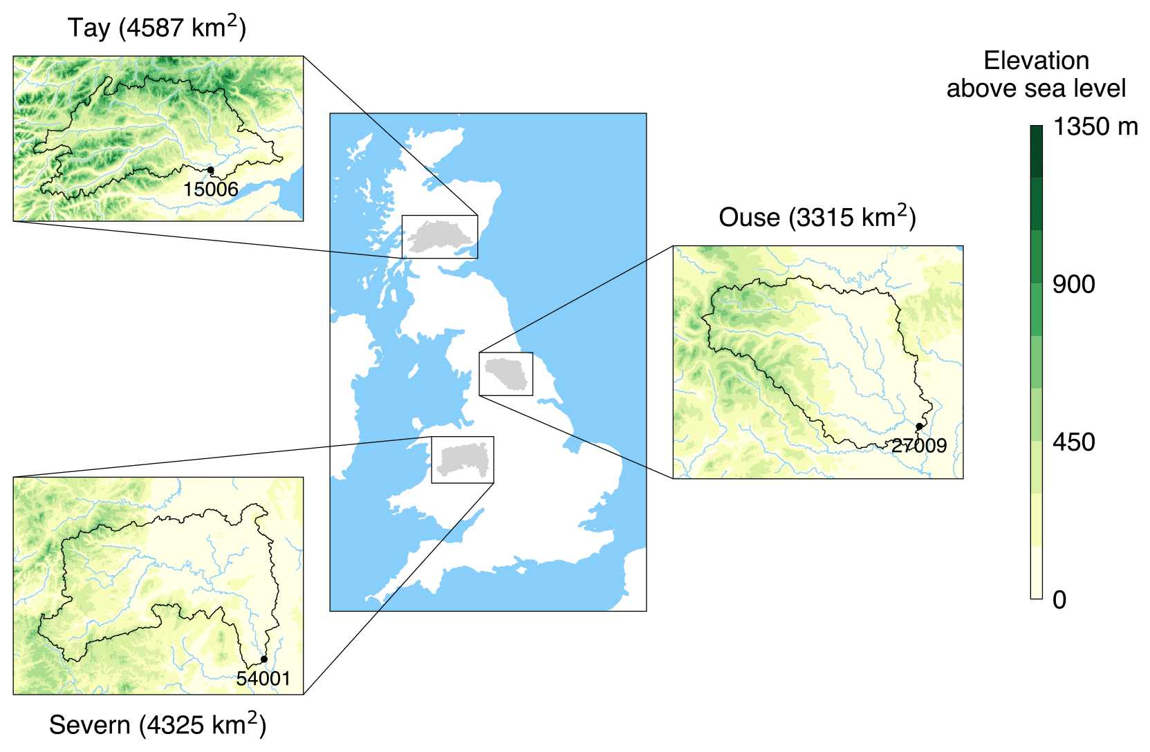
Figure 4Location of the three study catchments in Great Britain. In the zoomed-in panels, the dots correspond to the outlets of the catchments and their adjoining five-digit labels correspond to the number of the National River Flow Archive (NRFA) hydrometric stations at these outlets. The elevation is based on digital spatial data licensed from the UK Centre for Ecology & Hydrology, © UKCEH (Morris and Flavin, 1990, 1994).
5.4 Results
Figure 5 showcases the river discharge simulated with the three framework configurations described above, focussing on the river discharge at the catchment outlet in the line plots (a, c, e), and the spatial distribution of river discharge at the end of the simulation in the gridded plots (b, d). For reasons of brevity, only the Tay catchment is shown in the main text, figures for the other two study catchments are available in Appendix B. These figures qualitatively confirm the plausibility of the framework simulations. Indeed, the overlaid hydrographs suggest that the overall observed discharge pattern is captured by the simulations, while the spatial distributions of river discharge sketch a realistic picture of the catchment river network.
In addition, a quantitative evaluation of the performance of the framework simulations is done with respect to the river discharge at the catchment outlet where observed and simulated time series are compared using the non-parametric Kling–Gupta efficiency (RNP). This is a composite metric made of three equally weighted components, rS, αNP, and β, assessing the agreement in the dynamics (i.e. correlation), the variability, and the volume (i.e. bias) of the discharge time series, respectively (Pool et al., 2018). Table 3 features these metric components computed for the three configurations and the three study catchments using the Python package hydroeval (Hallouin, 2021).
The comparative performance of the three configurations for each catchment in turn informs the most suitable combination of components for a given temporal and geographical context. For instance, the third configuration appears to be the most suitable in the Tay catchment, if one is solely interested in simulating the river discharge accurately (RNP of 0.766), while the second configuration would be preferred for the Ouse and Severn catchments (RNP of 0.674 and 0.706, respectively). However, these conclusions are metric-dependent and the analysis of the components of the composite metric can reveal the strengths and weaknesses of a given configuration, e.g. while the third configuration performs highest on the composite metric in the Tay catchment, its ranking on capturing the flow variability is the lowest of the three configurations (αNP of 0.940).
Some caveats in this comparison are that the third configuration used a calibrated model unlike the first and second configurations, and the second configuration used data from a model constrained to conserve mass and energy, unlike the other configurations that only conserve mass. This likely skews the comparison.
This brief analysis of the results is used to demonstrate the potential of the framework to compare alternative combinations of components to simulate the hydrological behaviour for a given region and a given objective; it is not to draw definitive conclusions as to which combinations should be used for the catchments selected here, and more components than those presented in this paper can be developed and used in the framework. Moreover, this analysis focuses on one hydrological variable, the river discharge, but other hydrological variables such as e.g. soil moisture or evaporation could also be considered.
Table 3Quantitative comparison of the three configurations for the three study catchments.

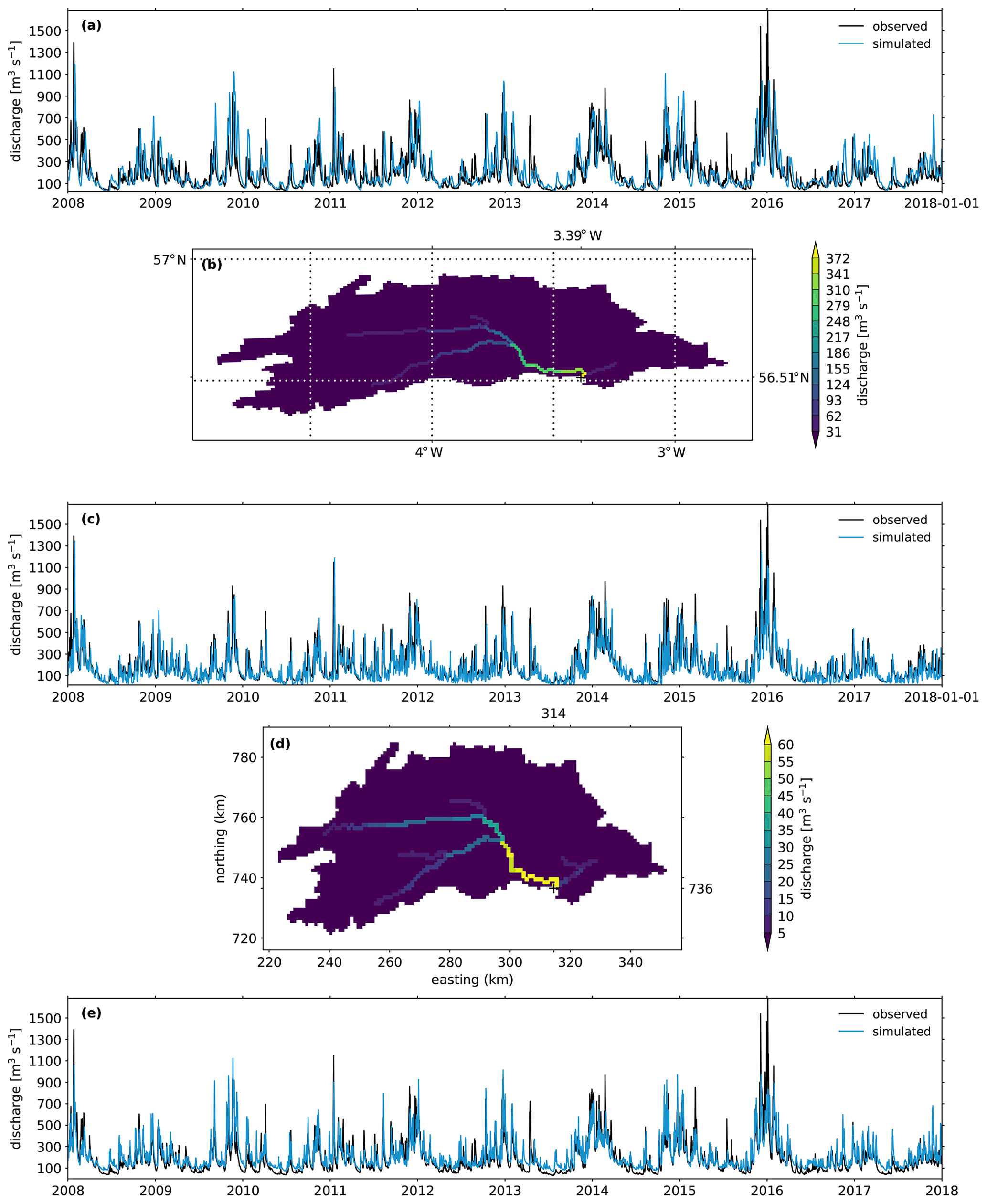
Figure 5Simulation of the river discharge with the three configurations for the Tay catchment: (a) observed and simulated hydrographs with configuration 1 at the catchment outlet (3.39∘ W, 56.51∘ N), (b) gridded simulated discharge with configuration 1 for the last simulation step (1 January 2018), (c) observed and simulated hydrographs with configuration 2 at the catchment outlet (314, 736), (d) gridded simulated discharge with configuration 2 for the last simulation step (1 January 2018), (e) observed and simulated hydrographs with configuration 3 at the catchment outlet.
The framework presented in this paper, the Unified Framework for Hydrology (UniFHy) represents the first implementation of a new modular blueprint to model the terrestrial water cycle. It is open source and comes with extended online documentation. By design, this Python package is intended to be easy to use, with a low entry bar for people with little programming experience. Indeed, installing a Python package is straightforward and only a few steps in a Python script are needed to set up and run a complete model in a Jupyter Notebook, which is likely to prove useful for teaching and training activities alike. It is also intended to be easily customisable, through choosing from a library of compatible science components those most suitable for a given modelling context. Finally, it is intended to be easily extensible by creating new components which should streamline the development and sharing of new science for the terrestrial water cycle.
In comparison to other hydrological and land surface modelling frameworks, this framework consciously reduces the degrees of freedom offered to the model developers in view to maximise the potential for reusability of their contributions with the other interested modelling communities. Indeed, unlike highly granular frameworks such as SUMMA or Raven, UniFHy prescribes the level of granularity to three modelling components, much like in Earth system modelling frameworks such as ESMF or OASIS-MCT. In addition, unlike other component-based modelling frameworks such as PyMT or Landlab, UniFHy prescribes the information to be exchanged between modelling components through its standardised interfaces. In addition, it controls the time advancement and the state memory allocation for the user which will be a crucial advantage when it is coupled in Earth system models. Nonetheless, UniFHy should be able to benefit directly from existing modelling environments such as Landlab, FUSE, or SUPERFLEX to develop modelling components.
In order to become the future of land components and improve the coarse-grained concurrency of Earth system models (Balaji et al., 2016; Lawrence et al., 2018), later versions of the framework will technically require the implementation of additional functionalities including implicit spatial heterogeneity such as tiling schemes (see e.g. nine surface types in JULES; Best et al., 2011; Clark et al., 2011) and hydrologically connected units (see e.g. flow matrix of TOPMODEL; Beven and Freer, 2001, in use in HydroBlocks; Chaney et al., 2016, intra-hillslope configuration in CLM; Swenson et al., 2019, unit-to-unit routing in ORCHIDEE; Nguyen-Quang et al., 2018); unstructured spatial meshes already in use in atmospheric models (see e.g. reduced grids in ECMWF's IFS model; Hortal and Simmons, 1991), icosahedral grids as in DWD's ICON model (Zängl et al., 2015) or IPSL's DYNAMICO core (Dubos et al., 2015), or cubed spheres as in UK Met Office's LFRic model (Adams et al., 2019), or NOAA's FV3 model (Putman and Lin, 2007); task and domain decomposition for parallel execution (such as in ESMF; Collins et al., 2005, OASIS-MCT; Valcke, 2013; Craig et al., 2017, or CPL7; Craig et al., 2012); and expose interfaces for coupling with external models (atmosphere and ocean). In addition, later versions of the framework will scientifically require an extension of the blueprint to include other biogeochemical cycles (e.g. carbon, nitrogen, phosphorus) as well as anthropogenic influences.
In the meantime, we hope that the science library will grow with new contributions from the land, hydrology, and groundwater modelling communities, and stimulate collaborations among them.
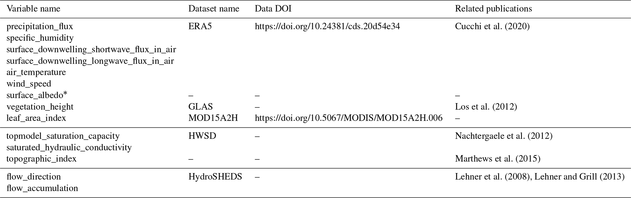
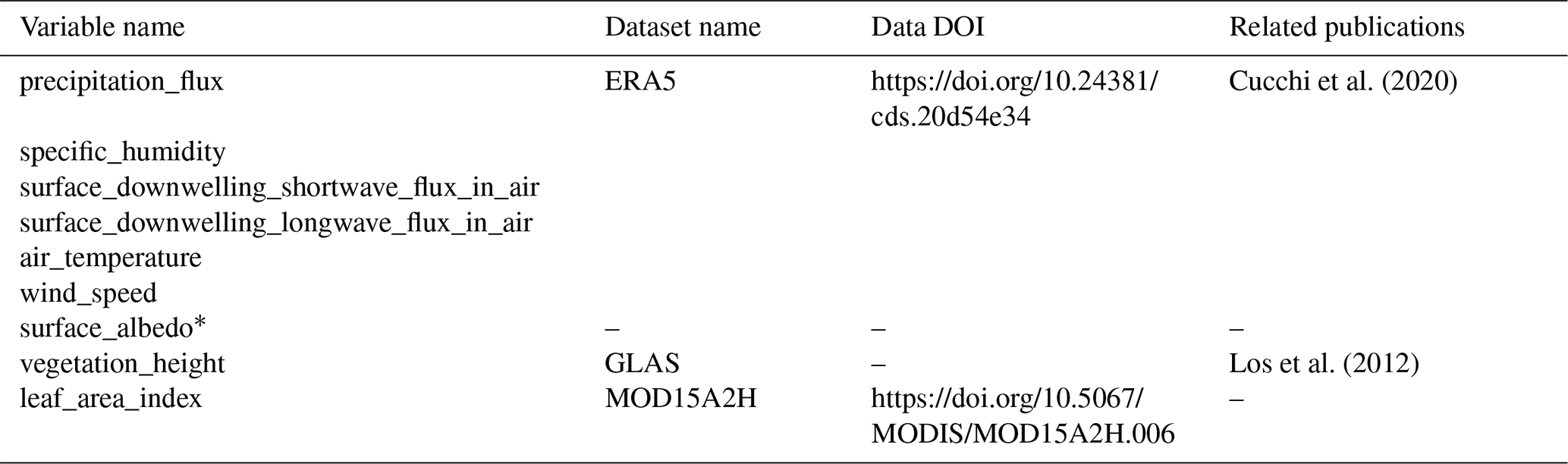
Table A1Sources for data used in configuration 1.
∗ Produced using suite u-ag343 accessible at https://code.metoffice.gov.uk/trac/roses-u (last access: 10 October 2021)

Table A3Sources for data used in configuration 3.
∗ Produced using suite u-ag343 accessible at https://code.metoffice.gov.uk/trac/roses-u (last access: 10 October 2021)
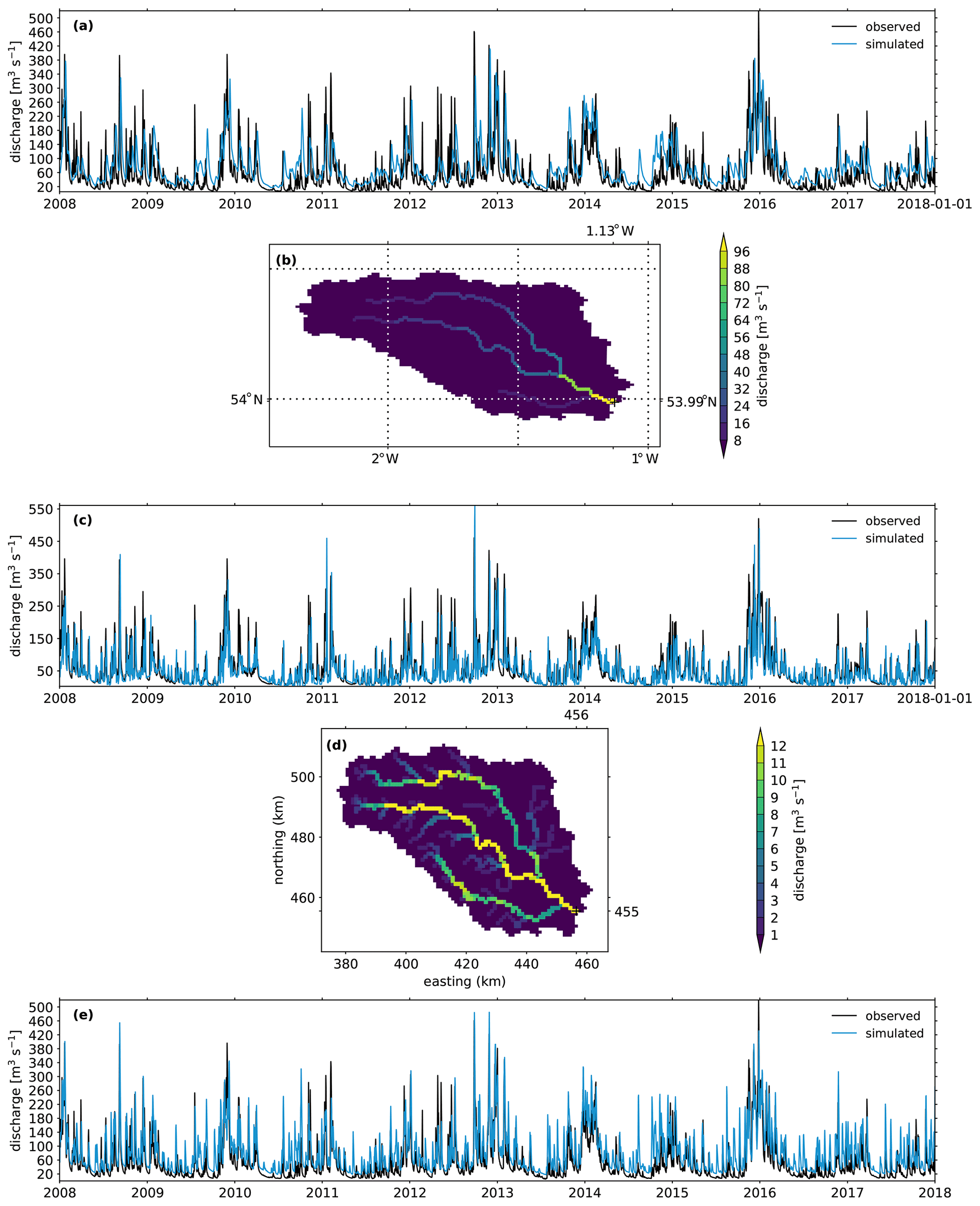
Figure B1Simulation of the river discharge with the three configurations for the Ouse catchment: (a) observed and simulated hydrographs with configuration 1 at the catchment outlet (1.13∘ W, 53.99∘ N), (b) gridded simulated discharge with configuration 1 for the last simulation step (1 January 2018), (c) observed and simulated hydrographs with configuration 2 at the catchment outlet (456, 455), (d) gridded simulated discharge with configuration 2 for the last simulation step (1 January 2018), (e) observed and simulated hydrographs with configuration 3 at the catchment outlet.
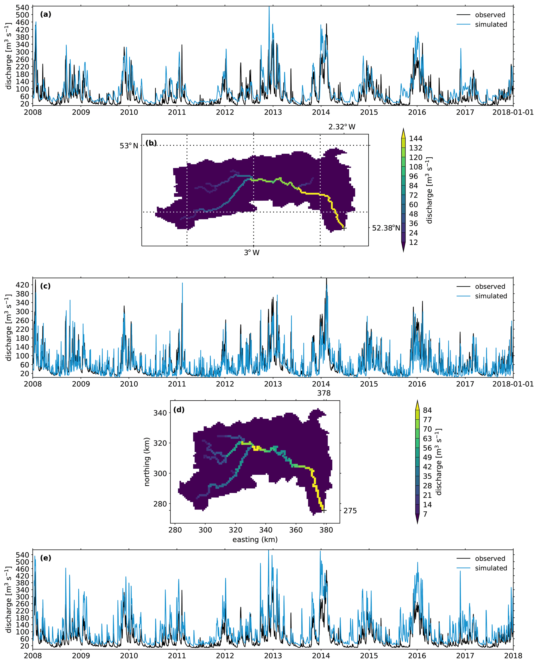
Figure B2Simulation of the river discharge with the three configurations for the Severn catchment: (a) observed and simulated hydrographs with configuration 1 at the catchment outlet (2.32∘ W, 52.38∘ N), (b) gridded simulated discharge with configuration 1 for the last simulation step (1 January 2018), (c) observed and simulated hydrographs with configuration 2 at the catchment outlet (378, 275), (d) gridded simulated discharge with configuration 2 for the last simulation step (1 January 2018), (e) observed and simulated hydrographs with configuration 3 at the catchment outlet.
The framework is open source and available on Zenodo (https://doi.org//10.5281/zenodo.6466215; Hallouin and Ellis, 2021). The science components are also open source and available on Zenodo, i.e. Artemis (https://doi.org/10.5281/zenodo.6560408; Dadson et al., 2021), RFM (https://doi.org/10.5281/zenodo.6466270; Lewis and Hallouin, 2021), and SMART (https://doi.org/10.5281/zenodo.6466276; Hallouin et al., 2021).
The input data used in the case studies are publicly available using the references provided in Appendix A. The observed river flow data are publicly available from National River Flow Archive (2021) (https://nrfa.ceh.ac.uk/data, last access: 10 October 2021). The framework output data are available upon request from the corresponding author.
The supplement related to this article is available online at: https://doi.org/10.5194/gmd-15-9177-2022-supplement.
All co-authors designed the blueprint for the framework. TH and RJE developed the framework implementation in Python. TH performed the simulations. TH and RJE processed the simulation outputs. TH prepared the manuscript with contributions from all co-authors.
The contact author has declared that none of the authors has any competing interests.
Publisher's note: Copernicus Publications remains neutral with regard to jurisdictional claims in published maps and institutional affiliations.
This work was undertaken through the Hydro-JULES research programme of the Natural Environment Research Council (NERC). AGH publishes with the permission of the Executive Director, British Geological Survey.
The authors would like to thank the developers of cf-python, David Hassell and Sadie Bartholomew, for implementing the requested features required by the framework, and Andy Heaps for the cf-plot support. They would also like to thank Katie Facer-Childs for providing the rainfall and potential evapotranspiration data used to calibrate the SMART model, Helen Davies for providing the HydroSHEDS dataset, and Huw Lewis for providing a Python version of RFM used to create an open water component for use in the framework.
The authors also thank the editor and the reviewers for their valuable comments and suggestions that contributed to improving the manuscript.
This research has been supported by the Natural Environment Research Council (grant no. NE/S017380/1).
This paper was edited by Dan Lu and reviewed by Ethan Coon and two anonymous referees.
Adams, S., Ford, R., Hambley, M., Hobson, J., Kavčič, I., Maynard, C., Melvin, T., Müller, E., Mullerworth, S., Porter, A., Rezny, M., Shipway, B., and Wong, R.: LFRic: Meeting the challenges of scalability and performance portability in Weather and Climate models, J. Parallel Distr. Com., 132, 383–396, https://doi.org/10.1016/j.jpdc.2019.02.007, 2019. a
Balaji, V., Benson, R., Wyman, B., and Held, I.: Coarse-grained component concurrency in Earth system modeling: parallelizing atmospheric radiative transfer in the GFDL AM3 model using the Flexible Modeling System coupling framework, Geosci. Model Dev., 9, 3605–3616, https://doi.org/10.5194/gmd-9-3605-2016, 2016. a
Barnhart, K. R., Hutton, E. W. H., Tucker, G. E., Gasparini, N. M., Istanbulluoglu, E., Hobley, D. E. J., Lyons, N. J., Mouchene, M., Nudurupati, S. S., Adams, J. M., and Bandaragoda, C.: Short communication: Landlab v2.0: a software package for Earth surface dynamics, Earth Surf. Dynam., 8, 379–397, https://doi.org/10.5194/esurf-8-379-2020, 2020. a
Bell, V. A., Kay, A. L., Jones, R. G., and Moore, R. J.: Development of a high resolution grid-based river flow model for use with regional climate model output, Hydrol. Earth Syst. Sci., 11, 532–549, https://doi.org/10.5194/hess-11-532-2007, 2007. a, b
Best, M. J., Beljaars, A., Polcher, J., and Viterbo, P.: A Proposed Structure for Coupling Tiled Surfaces with the Planetary Boundary Layer, J. Hydrometeorol., 5, 1271–1278, https://doi.org/10.1175/JHM-382.1, 2004. a
Best, M. J., Pryor, M., Clark, D. B., Rooney, G. G., Essery, R. L. H., Ménard, C. B., Edwards, J. M., Hendry, M. A., Porson, A., Gedney, N., Mercado, L. M., Sitch, S., Blyth, E., Boucher, O., Cox, P. M., Grimmond, C. S. B., and Harding, R. J.: The Joint UK Land Environment Simulator (JULES), model description – Part 1: Energy and water fluxes, Geosci. Model Dev., 4, 677–699, https://doi.org/10.5194/gmd-4-677-2011, 2011. a, b, c, d
Betts, A. K., Ball, J. H., Beljaars, A. C. M., Miller, M. J., and Viterbo, P. A.: The land surface-atmosphere interaction: A review based on observational and global modeling perspectives, J. Geophys. Res.-Atmos., 101, 7209–7225, https://doi.org/10.1029/95JD02135, 1996. a
Beven, K.: Rainfall-Runoff Modelling: The Primer, vol. 3204, Wiley-Blackwell, 2nd edn., https://doi.org/10.1002/9781119951001, 2012. a
Beven, K. and Freer, J.: A dynamic TOPMODEL, Hydrol. Process., 15, 1993–2011, https://doi.org/10.1002/hyp.252, 2001. a
Blyth, E. M., Arora, V. K., Clark, D. B., Dadson, S. J., De Kauwe, M. G., Lawrence, D. M., Melton, J. R., Pongratz, J., Turton, R. H., Yoshimura, K., and Yuan, H.: Advances in Land Surface Modelling, Current Climate Change Reports, 7, 45–71, https://doi.org/10.1007/s40641-021-00171-5, 2021. a, b, c
Boorman, D. B., Hollis, J. M., and Lilly, A.: Hydrology of soil types: a hydrologically-based classification of the soils of United Kingdom, Institute of Hydrology, Wallingford, ISBN 0 948540 69 9, 1995. a
Chaney, N. W., Metcalfe, P., and Wood, E. F.: HydroBlocks: a field-scale resolving land surface model for application over continental extents, Hydrol. Process., 30, 3543–3559, https://doi.org/10.1002/hyp.10891, 2016. a
Clark, D. B. and Gedney, N.: Representing the effects of subgrid variability of soil moisture on runoff generation in a land surface model, J. Geophys. Res.-Atmos., 113, D10111, https://doi.org/10.1029/2007JD008940, 2008. a
Clark, D. B., Mercado, L. M., Sitch, S., Jones, C. D., Gedney, N., Best, M. J., Pryor, M., Rooney, G. G., Essery, R. L. H., Blyth, E., Boucher, O., Harding, R. J., Huntingford, C., and Cox, P. M.: The Joint UK Land Environment Simulator (JULES), model description – Part 2: Carbon fluxes and vegetation dynamics, Geosci. Model Dev., 4, 701–722, https://doi.org/10.5194/gmd-4-701-2011, 2011. a, b, c, d
Clark, M. P., Slater, A. G., Rupp, D. E., Woods, R. A., Vrugt, J. A., Gupta, H. V., Wagener, T., and Hay, L. E.: Framework for Understanding Structural Errors (FUSE): A modular framework to diagnose differences between hydrological models, Water Resour. Res., 44, W00B02, https://doi.org/10.1029/2007WR006735, 2008. a
Clark, M. P., Fan, Y., Lawrence, D. M., Adam, J. C., Bolster, D., Gochis, D. J., Hooper, R. P., Kumar, M., Leung, L. R., Mackay, D. S., Maxwell, R. M., Shen, C., Swenson, S. C., and Zeng, X.: Improving the representation of hydrologic processes in Earth System Models, Water Resour. Res., 51, 5929–5956, https://doi.org/10.1002/2015WR017096, 2015a. a
Clark, M. P., Nijssen, B., Lundquist, J. D., Kavetski, D., Rupp, D. E., Woods, R. A., Freer, J. E., Gutmann, E. D., Wood, A. W., Brekke, L. D., Arnold, J. R., Gochis, D. J., and Rasmussen, R. M.: A unified approach for process-based hydrologic modeling: 1. Modeling concept, Water Resour. Res., 51, 2498–2514, https://doi.org/10.1002/2015WR017198, 2015b. a
Collins, N., Theurich, G., DeLuca, C., Suarez, M., Trayanov, A., Balaji, V., Li, P., Yang, W., Hill, C., and da Silva, A.: Design and Implementation of Components in the Earth System Modeling Framework, The International Journal of High Performance Computing Applications, 19, 341–350, https://doi.org/10.1177/1094342005056120, 2005. a, b, c
Craig, A., Valcke, S., and Coquart, L.: Development and performance of a new version of the OASIS coupler, OASIS3-MCT_3.0, Geosci. Model Dev., 10, 3297–3308, https://doi.org/10.5194/gmd-10-3297-2017, 2017. a, b
Craig, A. P., Vertenstein, M., and Jacob, R.: A new flexible coupler for earth system modeling developed for CCSM4 and CESM1, Int. J. High Perform. C., 26, 31–42, https://doi.org/10.1177/1094342011428141, 2012. a, b
Craig, J. R., Brown, G., Chlumsky, R., Jenkinson, R. W., Jost, G., Lee, K., Mai, J., Serrer, M., Sgro, N., Shafii, M., Snowdon, A. P., and Tolson, B. A.: Flexible watershed simulation with the Raven hydrological modelling framework, Environ. Model. Softw., 129, 104728, https://doi.org/10.1016/j.envsoft.2020.104728, 2020. a
Cucchi, M., Weedon, G. P., Amici, A., Bellouin, N., Lange, S., Müller Schmied, H., Hersbach, H., and Buontempo, C.: WFDE5: bias-adjusted ERA5 reanalysis data for impact studies, Earth Syst. Sci. Data, 12, 2097–2120, https://doi.org/10.5194/essd-12-2097-2020, 2020. a, b
Dadson, S., Bell, V., and Jones, R.: Evaluation of a grid-based river flow model configured for use in a regional climate model, J. Hydrol., 411, 238–250, https://doi.org/10.1016/j.jhydrol.2011.10.002, 2011. a, b
Dadson, S. J., Hallouin, T., and Ellis, R.: unifhycontrib-artemis, Zenodo [code], https://doi.org/10.5281/zenodo.6560408, 2021. a, b
Davies, H. N. and Bell, V. A.: Assessment of methods for extracting low-resolution river networks from high-resolution digital data, Hydrol. Sci. J., 54, 17–28, https://doi.org/10.1623/hysj.54.1.17, 2009. a
Dubos, T., Dubey, S., Tort, M., Mittal, R., Meurdesoif, Y., and Hourdin, F.: DYNAMICO-1.0, an icosahedral hydrostatic dynamical core designed for consistency and versatility, Geosci. Model Dev., 8, 3131–3150, https://doi.org/10.5194/gmd-8-3131-2015, 2015. a
Eaton, B., Gregory, J., Drach, B., Taylor, K., Hankin, S., Blower, J., Caron, J., Signell, R., Bentley, P., Rappa, G., Höck, H., Pamment, A., Juckes, M., Raspaud, M., Horne, R., Whiteaker, T., Blodgett, D., Zender, C., and Lee, D.: NetCDF Climate and Forecast (CF) Metadata Conventions, http://cfconventions.org/Data/cf-conventions/cf-conventions-1.8/cf-conventions.html (last access: 20 December 2022), 2020. a
Eyring, V., Bony, S., Meehl, G. A., Senior, C. A., Stevens, B., Stouffer, R. J., and Taylor, K. E.: Overview of the Coupled Model Intercomparison Project Phase 6 (CMIP6) experimental design and organization, Geosci. Model Dev., 9, 1937–1958, https://doi.org/10.5194/gmd-9-1937-2016, 2016. a
Farrell, P., Piggott, M., Pain, C., Gorman, G., and Wilson, C.: Conservative interpolation between unstructured meshes via supermesh construction, Comput. Method. Appl. M., 198, 2632–2642, https://doi.org/10.1016/j.cma.2009.03.004, 2009. a
Fenicia, F., Kavetski, D., and Savenije, H. H. G.: Elements of a flexible approach for conceptual hydrological modeling: 1. Motivation and theoretical development, Water Resour. Res., 47, W11510, https://doi.org/10.1029/2010WR010174, 2011. a
Fisher, R. A. and Koven, C. D.: Perspectives on the Future of Land Surface Models and the Challenges of Representing Complex Terrestrial Systems, J. Adv. Model. Earth Sy., 12, e2018MS001453, https://doi.org/10.1029/2018MS001453, 2020. a
Gash, J. H. C.: An analytical model of rainfall interception by forests, Q. J. Roy. Meteor. Soc., 105, 43–55, https://doi.org/10.1002/qj.49710544304, 1979. a
Hallouin, T.: hydroeval: an evaluator for streamflow time series in Python, Zenodo [code], https://doi.org/10.5281/zenodo.4709652, 2021. a
Hallouin, T. and Ellis, R. J.: unifhy, Funded by the Natural Environment Research Council (NERC) Hydro-JULES programme (NE/S017380/1)., Zenodo [code], https://doi.org/10.5281/zenodo.6466215, 2021. a, b
Hallouin, T., Mockler, E., and Bruen, M.: SMARTpy: Conceptual Rainfall-Runoff Model, Zenodo [code], https://doi.org/10.5281/zenodo.3376589, 2019. a
Hallouin, T., Mockler, E. M., and Bruen, M.: unifhycontrib-smart, Zenodo [code], https://doi.org/10.5281/zenodo.6466276, 2021. a, b
Hanke, M., Redler, R., Holfeld, T., and Yastremsky, M.: YAC 1.2.0: new aspects for coupling software in Earth system modelling, Geosci. Model Dev., 9, 2755–2769, https://doi.org/10.5194/gmd-9-2755-2016, 2016. a
Harpham, Q., Hughes, A., and Moore, R.: Introductory overview: The OpenMI 2.0 standard for integrating numerical models, Environ. Model. Softw., 122, 104549, https://doi.org/10.1016/j.envsoft.2019.104549, 2019. a, b
Hassell, D. and Bartholomew, S. L.: cfdm: A Python reference implementation of the CF data model, J. Open Source Softw., 5, 2717, https://doi.org/10.21105/joss.02717, 2020. a
Hassell, D., Gregory, J., Blower, J., Lawrence, B. N., and Taylor, K. E.: A data model of the Climate and Forecast metadata conventions (CF-1.6) with a software implementation (cf-python v2.1), Geosci. Model Dev., 10, 4619–4646, https://doi.org/10.5194/gmd-10-4619-2017, 2017. a
Hobley, D. E. J., Adams, J. M., Nudurupati, S. S., Hutton, E. W. H., Gasparini, N. M., Istanbulluoglu, E., and Tucker, G. E.: Creative computing with Landlab: an open-source toolkit for building, coupling, and exploring two-dimensional numerical models of Earth-surface dynamics, Earth Surf. Dynam., 5, 21–46, https://doi.org/10.5194/esurf-5-21-2017, 2017. a
Hock, R.: Temperature index melt modelling in mountain areas, J. Hydrol., 282, 104–115, https://doi.org/10.1016/S0022-1694(03)00257-9, 2003. a
Hortal, M. and Simmons, A. J.: Use of Reduced Gaussian Grids in Spectral Models, Mon. Weather Rev., 119, 1057–1074, https://doi.org/10.1175/1520-0493(1991)119<1057:UORGGI>2.0.CO;2, 1991. a
Hutton, E., Piper, M., Drost, N., Gan, T., Kettner, A., Overeem, I., Stewart, S., and Wang, K.: The Python Modeling Toolkit (PyMT), Zenodo [code], https://doi.org/10.5281/zenodo.4985222, 2021. a
Hutton, E. W., Piper, M. D., and Tucker, G. E.: The Basic Model Interface 2.0: A standard interface for coupling numerical models in the geosciences, J. Open Source Softw., 5, 2317, https://doi.org/10.21105/joss.02317, 2020. a, b
Kling, H., Fuchs, M., and Paulin, M.: Runoff conditions in the upper Danube basin under an ensemble of climate change scenarios, J. Hydrol., 424–425, 264–277, https://doi.org/10.1016/j.jhydrol.2012.01.011, 2012. a
Kraft, P., Vaché, K. B., Frede, H.-G., and Breuer, L.: CMF: A Hydrological Programming Language Extension For Integrated Catchment Models, Environ. Model. Softw., 26, 828–830, https://doi.org/10.1016/j.envsoft.2010.12.009, 2011. a
Krinner, G., Viovy, N., de Noblet-Ducoudré, N., Ogée, J., Polcher, J., Friedlingstein, P., Ciais, P., Sitch, S., and Prentice, I. C.: A dynamic global vegetation model for studies of the coupled atmosphere-biosphere system, Global Biogeochem. Cycles, 19, GB1015, https://doi.org/10.1029/2003GB002199, 2005. a, b
Lawrence, B. N., Rezny, M., Budich, R., Bauer, P., Behrens, J., Carter, M., Deconinck, W., Ford, R., Maynard, C., Mullerworth, S., Osuna, C., Porter, A., Serradell, K., Valcke, S., Wedi, N., and Wilson, S.: Crossing the chasm: how to develop weather and climate models for next generation computers?, Geosci. Model Dev., 11, 1799–1821, https://doi.org/10.5194/gmd-11-1799-2018, 2018. a
Lawrence, D. M., Fisher, R. A., Koven, C. D., Oleson, K. W., Swenson, S. C., Bonan, G., Collier, N., Ghimire, B., van Kampenhout, L., Kennedy, D., Kluzek, E., Lawrence, P. J., Li, F., Li, H., Lombardozzi, D., Riley, W. J., Sacks, W. J., Shi, M., Vertenstein, M., Wieder, W. R., Xu, C., Ali, A. A., Badger, A. M., Bisht, G., van den Broeke, M., Brunke, M. A., Burns, S. P., Buzan, J., Clark, M., Craig, A., Dahlin, K., Drewniak, B., Fisher, J. B., Flanner, M., Fox, A. M., Gentine, P., Hoffman, F., Keppel-Aleks, G., Knox, R., Kumar, S., Lenaerts, J., Leung, L. R., Lipscomb, W. H., Lu, Y., Pandey, A., Pelletier, J. D., Perket, J., Randerson, J. T., Ricciuto, D. M., Sanderson, B. M., Slater, A., Subin, Z. M., Tang, J., Thomas, R. Q., Val Martin, M., and Zeng, X.: The Community Land Model Version 5: Description of New Features, Benchmarking, and Impact of Forcing Uncertainty, J. Adv. Model. Earth Sy., 11, 4245–4287, https://doi.org/10.1029/2018MS001583, 2019. a
Lehner, B. and Grill, G.: Global river hydrography and network routing: baseline data and new approaches to study the world's large river systems, Hydrol. Process., 27, 2171–2186, https://doi.org/10.1002/hyp.9740, 2013. a
Lehner, B., Verdin, K., and Jarvis, A.: New Global Hydrography Derived From Spaceborne Elevation Data, Eos, Transactions American Geophysical Union, 89, 93–94, https://doi.org/10.1029/2008EO100001, 2008. a
Lewis, H. and Hallouin, T.: unifhycontrib-rfm, Zenodo [code], https://doi.org/10.5281/zenodo.6466270, 2021. a, b
Los, S. O., Rosette, J. A. B., Kljun, N., North, P. R. J., Chasmer, L., Suárez, J. C., Hopkinson, C., Hill, R. A., van Gorsel, E., Mahoney, C., and Berni, J. A. J.: Vegetation height and cover fraction between 60∘ S and 60∘ N from ICESat GLAS data, Geosci. Model Dev., 5, 413–432, https://doi.org/10.5194/gmd-5-413-2012, 2012. a, b
Marthews, T. R., Dadson, S. J., Lehner, B., Abele, S., and Gedney, N.: High-resolution global topographic index values for use in large-scale hydrological modelling, Hydrol. Earth Syst. Sci., 19, 91–104, https://doi.org/10.5194/hess-19-91-2015, 2015. a
Martínez-de la Torre, A., Blyth, E., and Robinson, E.: Water, carbon and energy fluxes simulation for Great Britain using the JULES Land Surface Model and the Climate Hydrology and Ecology research Support System meteorology dataset (1961–2015) [CHESS-land], [data set], https://doi.org/10.5285/c76096d6-45d4-4a69-a310-4c67f8dcf096, 2018. a, b
Martínez-de la Torre, A., Blyth, E. M., and Weedon, G. P.: Using observed river flow data to improve the hydrological functioning of the JULES land surface model (vn4.3) used for regional coupled modelling in Great Britain (UKC2), Geosci. Model Dev., 12, 765–784, https://doi.org/10.5194/gmd-12-765-2019, 2019. a
McKay, M. D., Beckman, R. J., and Conover, W. J.: A Comparison of Three Methods for Selecting Values of Input Variables in the Analysis of Output From a Computer Code, Technometrics, 42, 55–61, https://doi.org/10.1080/00401706.2000.10485979, 2000. a
Mockler, E. M., O'Loughlin, F. E., and Bruen, M.: Understanding hydrological flow paths in conceptual catchment models using uncertainty and sensitivity analysis, Comput. Geosci., 90, 66–77, https://doi.org/10.1016/j.cageo.2015.08.015, 2016. a
Monteith, J. L.: Evaporation and environment, Symposia of the Society for Experimental Biology, 19, 205–234, 1965. a
Moore, R. J., Bell, V. A., Austin, R. M., and Harding, R. J.: Methods for snowmelt forecasting in upland Britain, Hydrol. Earth Syst. Sci., 3, 233–246, https://doi.org/10.5194/hess-3-233-1999, 1999. a
Morris, D. G. and Flavin, R. W.: A digital terrain model for hydrology, in: Proc. 4th International Symposium on Spatial Data Handling, edited by: Brassel, K. and Kishimoto, H., 1, 250–262, Zurich, 1990. a
Morris, D. G. and Flavin, R. W.: Sub-set of UK 50 m by 50 m hydrological digital terrain model grids, NERC, Institute of Hydrology, Wallingford, https://www.ceh.ac.uk/cy/node/16318 (last access: 10 October 2021), 1994. a
Nachtergaele, F., van Velthuizen, H., Verelst, L., Wiberg, D., Batjes, N., Dijkshoorn, J., van Engelen, V., Fischer, G., Jones, A., Montanarella, L., Petri, M., Prieler, S., Teixeira, E., and Shi, X.: Harmonized World Soil Database (version 1.2), Food and Agriculture Organization of the UN, International Institute for Applied Systems Analysis, ISRIC - World Soil Information, Institute of Soil Science – Chinese Academy of Sciences, Joint Research Centre of the EC, 2012. a
National River Flow Archive: https://nrfa.ceh.ac.uk/data, National River Flow Archive [data set], last access: 10 October 2021. a
Nguyen-Quang, T., Polcher, J., Ducharne, A., Arsouze, T., Zhou, X., Schneider, A., and Fita, L.: ORCHIDEE-ROUTING: revising the river routing scheme using a high-resolution hydrological database, Geosci. Model Dev., 11, 4965–4985, https://doi.org/10.5194/gmd-11-4965-2018, 2018. a
Peckham, S. D., Hutton, E. W., and Norris, B.: A component-based approach to integrated modeling in the geosciences: The design of CSDMS, Comput. Geosci., 53, 3–12, https://doi.org/10.1016/j.cageo.2012.04.002, 2013. a, b
Polcher, J., McAvaney, B., Viterbo, P., Gaertner, M.-A., Hahmann, A., Mahfouf, J.-F., Noilhan, J., Phillips, T., Pitman, A., Schlosser, C., Schulz, J.-P., Timbal, B., Verseghy, D., and Xue, Y.: A proposal for a general interface between land surface schemes and general circulation models, Global Planet. Change, 19, 261–276, https://doi.org/10.1016/S0921-8181(98)00052-6, 1998. a
Pool, S., Vis, M., and Seibert, J.: Evaluating model performance: towards a non-parametric variant of the Kling-Gupta efficiency, Hydrol. Sci. J., 63, 1941–1953, https://doi.org/10.1080/02626667.2018.1552002, 2018. a
Putman, W. M. and Lin, S.-J.: Finite-volume transport on various cubed-sphere grids, J. Comput. Phys., 227, 55–78, https://doi.org/10.1016/j.jcp.2007.07.022, 2007. a
Smith, K. A., Barker, L. J., Tanguy, M., Parry, S., Harrigan, S., Legg, T. P., Prudhomme, C., and Hannaford, J.: A multi-objective ensemble approach to hydrological modelling in the UK: an application to historic drought reconstruction, Hydrol. Earth Syst. Sci., 23, 3247–3268, https://doi.org/10.5194/hess-23-3247-2019, 2019. a
Swenson, S. C., Clark, M., Fan, Y., Lawrence, D. M., and Perket, J.: Representing Intrahillslope Lateral Subsurface Flow in the Community Land Model, J. Adv. Model. Earth Sy., 11, 4044–4065, https://doi.org/10.1029/2019MS001833, 2019. a
Valcke, S.: The OASIS3 coupler: a European climate modelling community software, Geosci. Model Dev., 6, 373–388, https://doi.org/10.5194/gmd-6-373-2013, 2013. a, b
Zängl, G., Reinert, D., Rípodas, P., and Baldauf, M.: The ICON (ICOsahedral Non-hydrostatic) modelling framework of DWD and MPI-M: Description of the non-hydrostatic dynamical core, Q. J. Roy. Meteor. Soc., 141, 563–579, https://doi.org/10.1002/qj.2378, 2015. a
- Abstract
- Introduction
- Description of the framework
- Usage of the framework
- Contribution to the framework
- Case studies using the framework
- Conclusions
- Appendix A: Data sources
- Appendix B: Additional results
- Code availability
- Data availability
- Author contributions
- Competing interests
- Disclaimer
- Acknowledgements
- Financial support
- Review statement
- References
- Supplement