Predicting peak daily maximum 8 h ozone and linkages to emissions and meteorology in Southern California using machine learning methods (SoCAB-8HR V1.0)

The growing abundance of data is conducive to using numerical methods to relate air quality, meteorology and emissions to address which factors impact pollutant concentrations. Often, it is the extreme values that are of interest for health and regulatory purposes (e.g., the National Ambient Air Quality Standard for ozone uses the annual maximum daily fourth highest 8 h average (MDA8) ozone), though such values are the most challenging to predict using empirical models. We developed four different computational models, including the generalized additive model (GAM), multivariate adaptive regression splines, random forest, and support vector regression, to develop observation-based relationships between the fourth highest MDA8 ozone in the South Coast Air Basin and precursor emissions, meteorological factors and large-scale climate patterns. All models had similar predictive performance, though the GAM showed a relatively higher R² value (0.96) with a lower root mean square error and mean bias.

1 Introduction

Tropospheric ozone has proven to be one of the most difficult air pollutants to control, especially in the South Coast Air Basin (SoCAB) of California, which includes the city of Los Angeles and parts of four counties with a 2020 population exceeding 18 million. Exposure to ozone can be harmful to human health, leading to a variety of adverse outcomes, including premature mortality (U.S. EPA, 2020), climate warming and decreased agricultural production (Ainsworth et al., 2012; Hong et al., 2020). Ozone is formed by chemical reactions between volatile organic compounds (VOCs) and nitrogen oxides (NO_x) in the presence of sunlight (Seinfeld and Pandis, 2016). In addition to VOC and NO_x emissions, meteorology and large-scale climate patterns affect ozone (Aw and Kleeman, 2003; Blanchard et al., 2014; Gorai et al., 2015; Kelley et al., 2020; Kleeman, 2008; Lu et al., 2019; Mahmud et al., 2010; Mcglynn et al., 2018). As such, the resulting relationships among ozone, emissions and meteorology are complex and difficult to model accurately. However, the rise of machine learning methods, along with an increasingly long observational record, suggests that observation-based models can be used to understand those relationships. Since the 17th century statistics have been used to record information about the wealth and population in Europe (Porter, 1981). For example, William Petty, a British scientist and economist, estimated the census data of Ireland through statistics (Banta, 1987). While the application of statistics had been restricted to a few fields until the 19th century, it gradually extended to other areas since then including physics, astronomy and recently air quality (Porter, 1995). At their core, statistical models aim at approximating a relationship between dependent and independent variables, with regression being the most commonly used method, a term that was coined by British statistician Francis Galton back in 1885 when he studied the trend of heights within families (Galton, 1889, 1888; Benirschke, 2004). The method however precedes the name, with the use of regression starting years before the term was introduced, dating back to the beginning of the 19th century with linear regression being applied to questions in astronomy, such as determining orbits of comets, while the least-squares method attributed to Adrien-Marie Legendre and Carl Friedrich Gauss was developed in the early 1800s (Stephen, 1981; Agarwal and Sen, 2014). At the start of the 20th century, some statisticians introduced the idea of nonlinear regression, trying to explain more complex systems (Fisher, 1922). Since then, as computational capacity increased dramatically in the past few decades, regression analysis has been widely used in most scientific fields.

The US Environmental Protection Agency's (EPA) National Ambient Air Quality Standard (NAAQS) for ozone is based on the annual maximum daily fourth highest 8 h average (MDA8) ozone observations, which is an extreme statistic, and extreme statistics are often difficult to accurately predict using empirical modeling, though different approaches have been used for various purposes. For example, the US EPA adjusted the MDA8 ozone predictions with meteorological observations using generalized linear modeling (GLM) with natural spline smoothing functions in the R program to develop a generalized additive model (GAM) (Camalier et al., 2007; Wells et al., 2021) that meteorologically adjusts ozone trends to help isolate the impact of emissions. The GAM is an extension of the GLM, which was introduced in 1986 (Hastie and Tibshirani, 1986, 1990). It is more flexible than the GLM due to the smoothing functions on independent variables. Previous studies suggested the GAM was useful to deal with the nonlinear relationship between MDA8 ozone concentrations and meteorological indicators. About 40 % to 90 % of the variance of the MDA8 ozone concentrations could be explained at different sites with meteorologically adjusted GAMs (Aldrin and Haff, 2005; Blanchard et al., 2014, 2019; Camalier et al., 2007; Flynn et al., 2021; Gong et al., 2018, 2017; Hu et al., 2021; Huang et al., 2020; Jeong et al., 2020; Ma et al., 2020; McClure and Jaffe, 2018; Pearce et al., 2011; Gao et al., 2022). GAMs can assess each independent variable's contribution to the dependent variable. The multivariate adaptive regression splines (MARS) model (Friedman, 1991) has been used to model the nonlinear relationship between ozone concentrations and precursors' concentrations/meteorological factors, including the interactions between the independent indicators (García Nieto and Álvarez Antón, 2014; Roy et al., 2018). Support vector regression (SVR) is an extension of the support vector machine (SVM) (Drucker et al., 1996; Rodríguez-Pérez et al., 2017; Smola and Schölkopf, 2004). Past studies have shown that the SVR model with kernel functions can fit the nonlinear relationships between ozone concentrations and meteorological factors and can obtain accurate predictions (Liu et al., 2017; Luna et al., 2014; Rybarczyk and Zalakeviciute, 2018; Sotomayor-Olmedo et al., 2013; Vong et al., 2012). Random forest (RF) is a machine learning method (Tin Kam, 1995) derived from the traditional decision tree method. Compared to the traditional method, it is more accurate because it contains multiple decision trees. The RF model can be used to fit nonlinear relationships and deal with interaction effects. It can accurately predict ozone concentrations using meteorological variables and emissions and capture about 70 % to 95 % of the variability in ozone concentrations (Keller and Evans, 2019; Pernak et al., 2019; Stafoggia et al., 2020; Zhan et al., 2018). However, most prior empirical-model applications to simulate peak MDA8 ozone levels were biased low, especially when considering capturing the fourth highest annual MDA8 ozone concentrations.

In this study, we develop observation-based models (SoCAB-8HR V1.0) using four different methods (GAM, RF, SVR and MARS) with a broad range of potential independent indicators that impact ozone formation (e.g., precursors emissions, meteorological conditions, large-scale climate events, chemical reactions, seasonal variations and weekend effects) to predict the annual fourth highest MDA8 ozone in the SoCAB from 1990 to 2019. We assess and compare model performance and their applicability to help understand how emissions and meteorology, independently and combined, impact high ozone levels.

2 Methods and data

2.1 Methods

Brief descriptions of the four methods (GAM, MARS, RF and SVR) are provided below, and they are described in greater detail in the referenced material.

2.1.1 Generalized additive model (GAM)

A GAM uses flexible, nonlinear relationships defined between “knots” in the explanatory variables using smoothing functions (Hastie and Tibshirani, 1986, 1990). The knot is the point of the link of two polynomial curves (Wood, 2017). Since the GAM is an additive model, which means each indicator's function adds together to form the model equation, the indicators can have a variety of relationships with the response variable. The general form of the GAM is written as (Hastie and Tibshirani, 1986, 1990; Wood, 2011, 2017)

$$y=a+\sum _{i=\mathrm{1}}^{n}f\left(x_i\right)+e,$$

where a is the intercept, e is the error term, x refers to each independent indicator and f means the function applied to the predictors.

There are multiple choices of the functions based on the relationship between each independent and dependent variable, such as splines, linear functions and polynomials. Splines (often cubic) are commonly applied to capture nonlinear relationships. Cubic splines can provide a comparatively more flexible curve than low-order splines. In addition, a cubic spline can avoid overfitting with a smaller curviness and be more effective with less computational time than high-order splines. The basis function of a cubic spline is a third-order polynomial equation:

$$y_i=a_i\cdot x^{\mathrm{3}}+b_i\cdot x^{\mathrm{2}}+c_i\cdot x+d_i,$$

where a, b, c and d are the estimated coefficients of each basis function and the subscript i indicates the number of basis functions (equal to the number of knots). Based on the number of knots, several basis functions are built with different estimated coefficients. Each spline is given by the weighted sum of the basis functions. Three to five knots typically are sufficient in practice, and the knots are evenly distributed based on the percentiles of each indicator (Harrell, 2015). The “mgcv” package in the R program was used to build the GAM between the peak MDA8 ozone concentrations and indicators (Hastie, 1991; Hastie and Tibshirani, 1990, 1986; Wood, 2011, 2017).

2.1.2 Multivariate adaptive regression splines (MARS)

The MARS model is a nonparametric, multivariate, piecewise regression model that can be used to develop the nonlinear relationships between the dependent variable and a set of indicators (Friedman, 1991). Similar to the GAM, linear splines (referred to as “hinge functions”) are applied to independent variables in the MARS model. The resulting model is formed by a weighted sum of basis functions. The MARS model can deal with nonlinear relationships and provide a more flexible curve than simple linear regression models and polynomial regression models due to the linear splines between each pair of knots. It is simpler, and the resulting associations between the dependent and indicator variables are easier to interpret than the complex machine learning methods (e.g., random forest and neural network). The general equation of the MARS model is as follows (Friedman, 1991; Leathwick et al., 2006; Oduro et al., 2015; Roy et al., 2018):

$$y={\mathit{\beta }}_{\mathrm{0}}+\sum _{i=\mathrm{2}}{\mathit{\beta }}_i{H}_i,$$

where β₀ is the intercept, H_i shows hinge functions and β_i is the coefficients of hinge functions. The hinge functions in the MARS model are pairwise, and the form is

$$\begin{array}{c}{\displaystyle }(x-k{)}_{+}=max(x-k,\mathrm{0}),\\ {\displaystyle }(k-x{)}_{+}=max(k-x,\mathrm{0}),\end{array}$$

where k is the knot. When applying the MARS model, a two-stage approach is used that includes forward and backward stages. The forward stage is similar to the forward stepwise regression. At first, the model only includes the intercept term. Then, the generated pairwise hinge functions are added into the model continuously if they can reduce the residual error of the model. This process will be terminated when the change of error is small (e.g., less than a threshold) or the model reaches the defined maximum number of terms. A backward stage is applied to avoid overfitting and reduce the number of terms, removing terms that do not significantly impact the error (Wikipedia Contributors, 2022). Generalized cross validation (GCV) is used to find the final MARS model after obtaining multiple models that have different terms (Friedman, 1991; Friedman and Silverman, 1989; Hastie and Tibshirani, 1996; Leathwick et al., 2006; Oduro et al., 2015; Roy et al., 2018). The “earth” package in R was applied to build the relationship between the top MDA8 ozone concentrations and independent indicators using the MARS model (Friedman and Silverman, 1989; Milborrow, 2021; Hastie et al., 2009), and this package chose the independent variables, the position of the knots and the interaction of the terms automatically.

2.1.3 Random forest model (RF)

Random forest is a supervised machine learning method that can be used for regression and classification. It is an ensemble of multiple decision trees. The RF model resolves the limitation of the decision tree that the model can be overfitting if the depth of the trees is deeper by applying the bagging algorithm. The bagging algorithm effectively reduces the variance of the model results and makes the RF model quite stable and robust. In regression, the predicted result of the RF model is the average of the results of all decision trees. The total error of RF is computed by the average of the error of all the decision trees.

Suppose we build a random forest model which contains m trees (i.e., T_b, $b=\mathrm{1},\mathrm{2},\mathrm{\dots },m$) and has a testing point x. The predicted value of input x would be

$${\displaystyle \frac{\mathrm{1}}{m}}\sum _{i=\mathrm{1}}^m{T}_i\left(x\right).$$

The following steps construct each decision tree in a random forest model. First, randomly select a subset of the training dataset with replacement. Then, at each decision node, randomly select a subset of variables. In order to find the optimal variable and its corresponding value that can lead to the best fit, we usually define a target function and compare all variables in the subset to find the variable with the lowest or highest value. Once we find the optimal variable and corresponding value, we next divide the decision node based on the optimal variable and value. Repeat the previous step until all decision nodes reach the minimal node size. Finally, for each leaf node, suppose k data points, $x_{\mathrm{1}}{x}_{\mathrm{2}},\mathrm{\dots },x_k$, belong to a leaf node and the corresponding response variables are $y_{\mathrm{1}}{y}_{\mathrm{2}},\mathrm{\dots },y_k$ respectively. The predicted result of a testing point x which falls into this leaf node should be

$${\displaystyle \frac{\mathrm{1}}{k}}\sum _{i=\mathrm{1}}^k{y}_i.$$

We used the “randomForest” package in the R software to build the RF model (Liaw and Wiener, 2002). RF models can select interaction terms between the independent variables automatically.

2.1.4 Support vector regression (SVR)

The support vector machine (SVM) method is a supervised machine learning approach that is used for classification. The SVR model, which is an extension of the SVM, can be used to describe the nonlinear relationships between the response variable and independent indicators.

Suppose we have a set of indicators $X=\mathit{\{}{x}_{\mathrm{1}}{x}_{\mathrm{2}},\mathrm{\dots },x_m\mathit{\}}$ and a set of response variables $Y=\mathit{\{}{y}_{\mathrm{1}}{y}_{\mathrm{2}},\mathrm{\dots },y_m\mathit{\}}$. We need to find a hyperplane to minimize error and achieve the best fit, which can be written as w^Tx+b. We can define the loss function as

$$\text{Loss}\left(x_i,y_i\right)=max(\mathrm{0},\mathrm{|}{w}^T{x}_i+b-y_i\mathrm{|}-\mathit{\epsilon }),$$

where ε (epsilon) is the margin of error, a user-defined variable that can be manipulated to adjust the accuracy of the model. Then, the problem can be written as

$$\underset{w,b}{min}{\displaystyle \frac{\mathrm{1}}{\mathrm{2}}}{∥w∥}^{\mathrm{2}}+C\sum _{i=\mathrm{1}}^m\text{Loss}(x_i,y_i),$$

where C is the cost, another user-defined variable that determines the tolerance of the model to points outside the bounds set by ε, and m is the number of dataset. To let the loss function result of each training point be 0, we introduced the slack variables. Then, the development of a nonlinear relationship between the response variable and indicators can be converted a Lagrangian dual problem (Schölkopf and Smola, 2001; Smola and Schölkopf, 2004).

We need to consider the interactions among features sometimes when we build computational models, so we need to map the data into a nonlinear feature space. The nonlinear feature space increases the dimension of the data space, and consequently the computational complexity grows dramatically. We introduced a kernel function to account for the interactions and reduce the computational complexity. We used the package “e1071” in R software to build the SVR model (Chang and Lin, 2011; Fan et al., 2005).

2.2 Model evaluation

We used the coefficient of determination (R²), mean bias (MB) and root mean squared error (RMSE) of the observed and predicted peak MDA8 ozone concentrations from 1990 to 2019 to compare the performance of these four models.

$$\begin{array}{c}{\displaystyle }\text{Mean bias}={\displaystyle \frac{\sum _{i=\mathrm{1}}^n({\widehat{x}}_i-x_i)}{n}},\\ {\displaystyle }\text{RMSE}=\sqrt{{\displaystyle \frac{\sum _{i=\mathrm{1}}^n(x_i-{\widehat{x}}_i{)}^{\mathrm{2}}}{n}}},\end{array}$$

where x_i and ${\widehat{x}}_i$ are the observed and predicted MDA8 ozone concentrations and n is the total number of measurements. In addition, we used 10-fold cross validation (CV) to evaluate the prediction accuracy and stability of these four models. In the 10-fold CV, the dataset is randomly divided into two subsets, in which 90 % is used to train the model and 10 % is the testing dataset. These two subsets are not overlapped, and this separation process repeats 10 times. The averages of the R², MB and RMSE in these 10 runs are the final evaluation results of numerical models.

2.3 Study domain

The SoCAB includes urban and suburban parts of Los Angeles County, Riverside County and San Bernardino County and all of Orange County. This area historically and still experiences some of the worst air quality in the US, and various air pollutants at multiple sites in the SoCAB do not meet the NAAQS, even with strict regulations leading to significant reductions in pollutant emissions. The poor air quality is because SoCAB is one of the most urbanized and populated regions in the US and is surrounded by mountains on three sides, while the Pacific Ocean lies on the west side. Temperature inversions are formed frequently along the coast due to the warm subsiding air from North Pacific highs, suppressing vertical mixing. This unique geographical and meteorological environment leads to reduced dilution of air pollutants. In addition, most days in a year are sunny, leading to warm and dry conditions with high solar radiation, exacerbating the formation of photochemically derived pollutants, such as ozone.

We first focused on the Crestline site to develop the initial regression models to predict the fourth highest MDA8 ozone concentrations in the SoCAB. This site had the annual fourth highest MDA8 ozone concentrations during about 77 % of this project's period. The other 23 % of the time, the maximum site was close to the Crestline site, such as Glendora, Redlands and Fontana.

2.4 Data

The daily MDA8 ozone concentrations from 1990 to 2019 in the South Coast Air Basin was retrieved from California Air Resources Board (CARB) archives and EPA Air Quality System (AQS) pre-generated data files (CARB, 2020). The total number of days of daily MDA8 ozone levels is 10 957. We used the top 30 MDA8 ozone days each year to develop the models for the fourth highest MDA8 ozone concentrations to build robust computational models, since multiple factors have impacts on the peak MDA8 ozone concentrations. Significant factors may be missed if only the fourth highest MDA8 ozone concentrations are considered, such as the day of the year, day of the week and meteorological-variable impacts, as there would only be 30 observations for model training. Furthermore, the size of the 30 years' fourth highest MDA8 ozone dataset is too small to have sufficient statistical power. A small dataset may cause a type II error (failing to identify a statistically significant effect) for some significant features, which would then affect the accuracy of the predictions.

We selected 25 independent indicators, including precursors' emissions, meteorological factors suggested in previous studies (Blanchard et al., 2014, 2019; Camalier et al., 2007), Niño 3.4 monthly indices, the day of the week and the day of the year. A detailed description of all the variables applied to test the final computational models is in Table S1 in the Supplement.

Estimated NO_x and VOC emissions in the SoCAB from 2000 to 2019 were acquired from CARB archives using the emissions in 2012 (Cox et al., 2013). The emissions between 1990 and 2000 were projected with the emissions in 2008 and 2012 (Cox et al., 2009, 2013). The detailed calculation is in the Supplement.

We included two kinds of meteorological data: surface meteorological data and upper-air meteorological data. We obtained the surface meteorological data, including temperature, wind speed and wind direction at Los Angeles International Airport (LAX) and Barstow-Daggett Airport (Barstow Airport) from National Oceanic and Atmospheric Administration (NOAA) archives and CARB archives (Menne et al., 2012a, b). The upper-air meteorological data at the Miramar site was provided by NOAA and contains geopotential height, temperature, dew point temperature, wind speed and wind direction at 500 and 850 mb (millibar). Using temperature and dew point temperature, we computed the relative humidity (RH) at 500 and 850 mb with the Clausius–Clapeyron equation (Alduchov and Eskridge, 1996; Lawrence, 2005). The height of 500 mb is around 5500 m (NOAA, 2020), and the 850 mb height is about 1500 m, which is close to the boundary layer height. The upper-air meteorology is related to the synoptic-scale weather and has an impact on the surface meteorology (Blanchard et al., 2014; Camalier et al., 2007).

Past studies have shown there is a relationship between the El Niño–Southern Oscillation (ENSO) events and the variability of MDA8 ozone concentrations by affecting the local meteorology (Lu et al., 2019; Oman et al., 2013, 2011; Xu et al., 2017). Niño 3.4 monthly indices were obtained from the Climate Prediction Center (CPC) to represent ENSO events. To account for the daily variations and weekend effects of MDA8 ozone levels, we included the day of the week and the day of the year in the models (Seinfeld and Pandis, 2016).

3 Results

3.1 Model application and performance

3.1.1 GAM model

We combined stepwise regression and F values to assess the statistical significance of each independent indicator to refine the model equation to provide the smallest Akaike information criterion (AIC) value after excluding the highly correlated indicators (Fig. S1) (Pope and Webster, 1972). However, the stepwise regression may exclude some factors that are known to be tied to ozone formation from the final equation, including VOC emissions, the day of the year and the day of the week. We used both statistical indicators and knowledge of important relationships in the final model to avoid losing significant factors that affect the peak ozone levels. Furthermore, a limitation of the GAM is that it does not identify interaction terms, so interaction terms were introduced with the spline function manually in the style of s(x1,x2).

We applied cubic splines to the emissions and meteorological variables due to the nonlinear relationship between peak MDA8 ozone concentrations and meteorology/emissions. Also, the cubic spline was used for the day of the year to add the daily and seasonal variation of the precursors' emissions. In addition, we included the day of the week in a factor style to represent the weekend effect and Niño 3.4 monthly indices to show the large-scale climate pattern impacts on ozone formation with linear functions. We used the annual top 30 MDA8 ozone concentrations from 1990 to 2019 on a log scale as the dependent variable at the Crestline site because the ozone concentrations follow a log-normal distribution (U.S. EPA, 2020; Henneman et al., 2015; Hogrefe et al., 2000; Rao et al., 1997; Blanchard et al., 2014; Camalier et al., 2007).

The final GAM (GAM-SoCAB-8HR V1.0) included emissions, meteorological factors, large-scale climate indices and temporal variables at the Crestline site from 1990 to 2019 (Eq. 1). The detailed description of each variable is in Table 1 (e: error term):

$$\begin{array}{}\text{(1)}& \begin{array}{rl}\log \left(\text{MDA8}\right)& =a+\text{dayofweek (factor)}+\text{dayofyear}\\ & +s\left(\text{TMAXBarstow}\right)+s\left(\mathrm{Mir}\mathrm{850}\mathrm{RH}\right)\\ & +s\text{(AWNDLAX)}+s\left(\mathrm{e}{\mathrm{NO}}_x\right)+s\text{(eROG)}\\ & +s(\mathrm{e}{\mathrm{NO}}_x,\text{TMAXBarstow})\\ & +s\text{(eROG,TMAXBarstow)}\\ & +s(\mathrm{e}{\mathrm{NO}}_x,\text{eROG})+\text{ENSOmonthly}+\mathrm{e}.\end{array}\end{array}$$

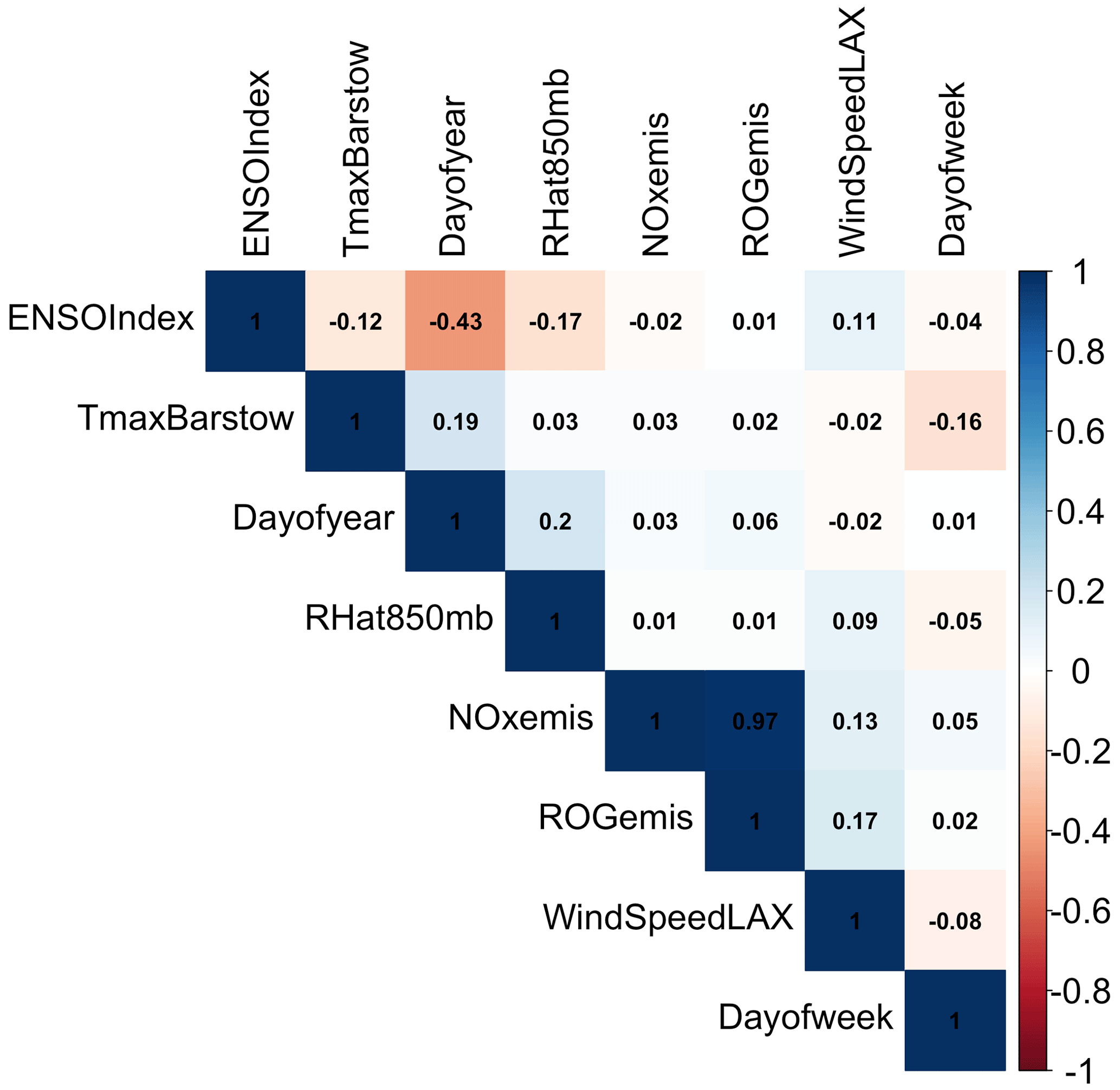
The correlation (R²) between independent variables in the final GAM was tested (Fig. 1). The correlation between VOC and NO_x emissions was high at close to 1. However, both are the precursors of MDA8 ozone, so these factors were not removed during the model development. Other than emissions, the correlation among all the significant independent variables in the final models is negligible (Fig. 1).

A total of 84 % of the variability of the peak MDA8 ozone concentrations can be explained using this GAM (Fig. 2a). The 10-fold validation results show that the R² value was 0.85 using the testing dataset, only 0.01 higher than the training dataset. Also, the RMSE of the testing data was only slightly different from that of the training data (Table S4), which indicated that this GAM could predict peak MDA8 ozone concentrations stably. This model had an R² value equal to 0.96, and RMSE is 11.1 ppbv for the fourth highest MDA8 ozone predictions from 1990 to 2019 (Fig. 3a).

Figure 1 Correlation value between the independent variables (only valid for GAM).

3.1.2 MARS model

We used the same dataset as the GAM (GAM-SoCAB-8HR V1.0) to be comparable with the GAM's results. The final model contained six indicators, including the NO_x and VOC emissions, the maximum temperature at Barstow-Daggett Airport, the average wind speed at LAX, Niño 3.4 monthly indices, the day of the year and 11 interaction terms between indicators. Similar to GAM, we applied the log function to the ozone concentrations (Epa, 2020; Henneman et al., 2015; Hogrefe et al., 2000; Rao et al., 1997). The final equation of the MARS model (MARS-SoCAB-8HR V1.0) is shown below (Eq. 2). A detailed description of each variable is in Table 1:

$$\begin{array}{}\text{(2)}& \begin{array}{rl}\log \left(\text{MDA8}\right)& =\mathrm{4.59}+(\mathrm{1135.1}-\mathrm{e}{\mathrm{NO}}_x)\\ & \cdot (-\mathrm{9.57}\times {\mathrm{10}}^{-\mathrm{4}})\\ & +(\mathrm{e}{\mathrm{NO}}_x-\mathrm{1135.1})\cdot (\mathrm{1.55}\times {\mathrm{10}}^{-\mathrm{3}})\\ & +(\mathrm{643.4}-\text{eROG})\cdot (\mathrm{2.67}\times {\mathrm{10}}^{-\mathrm{3}})\\ & +(\text{TMAXBarstow}-\mathrm{36.7})\cdot \mathrm{0.022}\\ & +(\mathrm{1135.1}-\mathrm{e}{\mathrm{NO}}_x)\cdot (\text{eROG}-\mathrm{450.7})\\ & \cdot (\mathrm{4.29}\times {\mathrm{10}}^{-\mathrm{6}})+(\mathrm{e}{\mathrm{NO}}_x-\mathrm{1415.8})\\ & \cdot (\text{eROG}-\mathrm{643.4})\cdot (-\mathrm{1.08}\times {\mathrm{10}}^{-\mathrm{6}})\\ & +(\mathrm{e}{\mathrm{NO}}_x-\mathrm{1225})\cdot (\text{TMAXBarstow}-\mathrm{36.7})\\ & \cdot (\mathrm{7.21}\times {\mathrm{10}}^{-\mathrm{4}})+(\mathrm{1081.5}-\text{eROG})\\ & \cdot (\text{TMAXBarstow}-\mathrm{36.7})\cdot (-\mathrm{2.18}\times {\mathrm{10}}^{-\mathrm{5}})\\ & +(\text{eROG}-\mathrm{1081.5})\\ & \cdot (\text{TMAXBarstow}-\mathrm{36.7})\cdot (-\mathrm{3.95}\times {\mathrm{10}}^{-\mathrm{4}})\\ & +(\text{eROG}-\mathrm{643.4})\cdot (\mathrm{2.8}-\text{AWNDLAX})\\ & \cdot (-\mathrm{3.34}\times {\mathrm{10}}^{-\mathrm{4}})+(\text{eROG}-\mathrm{643.4})\\ & \cdot (\text{AWNDLAX}-\mathrm{2.8})\cdot (-\mathrm{4.99}\times {\mathrm{10}}^{-\mathrm{5}})\\ & +(\mathrm{26.91}-\text{ENSOmonthly})\\ & \cdot (\text{eROG}-\mathrm{643.4})\cdot (-\mathrm{3.03}\times {\mathrm{10}}^{-\mathrm{4}})\\ & +(\mathrm{28.3}-\text{ENSOmonthly})\\ & \cdot (\text{eROG}-\mathrm{1081.5})\cdot (-\mathrm{1.61}\times {\mathrm{10}}^{-\mathrm{3}})\\ & +(\mathrm{28.3}-\text{ENSOmonthly})\\ & \cdot (\text{eROG}-\mathrm{982.7})\cdot (\mathrm{1.34}\times {\mathrm{10}}^{-\mathrm{3}})\\ & +(\mathrm{235}-\text{dayofyear})\\ & \cdot (\text{TMAXBarstow}-\mathrm{36.7})\cdot (\mathrm{1.22}\times {\mathrm{10}}^{-\mathrm{4}}).\end{array}\end{array}$$

The R² when applied to predict the top 30 MDA8 ozone predictions was 0.83 and showed no overfitting (Table S4). The model also had a high R² (0.95), and RMSE equaled 11.2 ppbv when predicting the fourth highest MDA8 ozone concentrations (Fig. 3b).

Multiple tests were performed using the different number of the remaining terms in the output model with 10-fold CV to improve the MARS model performance. The best model was obtained when there were 14 terms maintained in the MARS model (Fig. S2). The performance of the MARS model with 14 terms (R²=0.83, RMSE = 10.19) was similar to the MARS model with 16 terms (R²=0.83, RMSE = 10.27).

3.1.3 RF model

We first applied the same indicators and dataset as the GAM (GAM-SoCAB-8HR V1.0) in order to compare the results of the above two regression methods. In the base case run, we tried 0–500 trees to find the optimal number of trees. Each tree chose two variables randomly that was equal to one-third of the total number of variables by default. The optimal number of trees was 467 based on the RMSE value (Fig. S3). The majority of the top 30 and fourth highest MDA8 ozone concentrations can be explained by the RF model (RF-SoCAB-8HR V1.0) (R²=0.81 and RMSE = 10.9 ppbv for the top 30 MDA8 ozone concentrations and R²=0.97 and RMSE = 14.0 ppbv for the fourth highest MDA8 ozone concentration; Figs. 2c and 3c). The R² and RMSE values of the 10-fold CV results were similar to those using the original RF model, with only a 0.01 difference in R² and about a 5 % reduction of the RMSE value that indicated this RF model had a high prediction accuracy and no overfitting (Table S4).

Two main hyperparameters affect the performance of RF models and can be tuned: the number of trees used in the RF model and the number of random variables in each tree. To improve the model performance further, we created a grid with hyperparameters that the number of indicators considered at each split from 2 to 8, and the number of trees was 1000 to tune the RF. The optimal number of predictors in each tree was 2 due to the lowest out-of-bag (OOB) error, the same as the default run. Also, the optimal number of trees after model tuning was the same as the default run.

Next, we included all the available indicators in the RF model after excluding the strongly correlated independent variables. Then we removed the statistically insignificant indicators based on the p value and the variable importance to find the optimal combination of independent variables in the RF model. The final model contained two more variables than the one above: maximum solar radiation and height at 850 mb. The importance of the additional variables was minor and had negligible impacts on the model performance (Fig. 4c). The optimal number of trees was equal to 495. The R² and RMSE values for the top 30 MDA8 ozone predictions were similar to those using the RF model with fewer variables, although the mean bias was reduced (Table S3). In addition, the model performance for the fourth highest MDA8 ozone predictions was worse than that using the RF model with the same variables as GAM (Table 2). Therefore, the RF model with the same GAM's variables fit the peak and the annual fourth highest MDA8 ozone concentrations well.

3.1.4 SVR model

We first built the SVR model (SVR-SoCAB-8HR V1.0) using the same variables as the built GAM (GAM-SoCAB-8HR V1.0) above with the default setting (the cost was 1, and epsilon was 0.1). We used kernel functions to consider the interactions between the independent indicators. Several kernel functions have been used in machine learning models, including the linear kernel, polynomial kernel, radial kernel, etc. In practice, we used the linear kernel for the linear relationship and the radial kernel for the nonlinear relationship. Owing to the nonlinear relationship between the peak MDA8 ozone levels and emissions/meteorology, we applied the radial kernel to the independent variables. The regression method we used was epsilon regression, and the epsilon value is related to the margin tolerance.

The R² and RMSE values of the top 30 MDA8 ozone predictions were very similar to the RF model's results, but the MB was larger than that of the RF model (Table S3). Results for predicting the fourth highest MDA8 ozone predictions found that the method did not capture the variability as well as the other methods (R²=0.89 and RMSE = 14.0 ppbv). The CV results indicated that this SVR model is stable and has no overfitting (Table S4).

Two parameters significantly impact the improvement of predictions and can be defined by users: the value of cost and epsilon. So we ran the SVR model with a hyperparameter grid with the cost value from 1 to 512 and the epsilon from 0 to 1 with an interval of 0.1. The model achieved the best performance when the epsilon was 0.3, and the cost was 1. The predicted top 30 and fourth highest MDA8 ozone concentrations were similar to those using the built SVR with default settings (Tables 2 and S3, Fig. S5).

We then built the SVR model with all the independent variables we had and removed the insignificant variables using the p value and variable importance. The optimal SVR model (SVRoptimal-SoCAB-8HR V1.0) contained the variables in the above GAM and height at 850 mb and maximum solar radiation. The ideal epsilon value was 0.1, and the cost value was 1, the same as the default setting. Though the importance of these two additional variables was close to 0, the model performance of simulations of the top 30 MDA8 ozone days improved slightly (R²=0.83 and RMSE = 10.4 ppbv) (Fig. 4d and Table S3). However, the fourth highest MDA8 ozone predictions were less accurate compared to the R² and RMSE using this SVR model (SVRoptimal-SoCAB-8HR V1.0) and the SVR model (SVR-SoCAB-8HR V1.0) with the same GAM variables (R²=0.87 and RMSE = 14.3 ppbv for the SVRoptimal-SoCAB-8HR V1.0 and R²=0.89 and RMSE = 14.0 ppbv for the SVR-SoCAB-8HR V1.0) (Table 2).

Figure 2 Comparison between the top 30 observed and predicted MDA8 ozone concentrations using the GAM-SoCAB-8HR V1.0 model (a), MARS-SoCAB-8HR V1.0 model (b), RF-SoCAB-8HR V1.0 model (c), SVR-SoCAB-8HR V1.0 model (d) and the SVRoptimal-SoCAB-8HR V1.0 model (e).

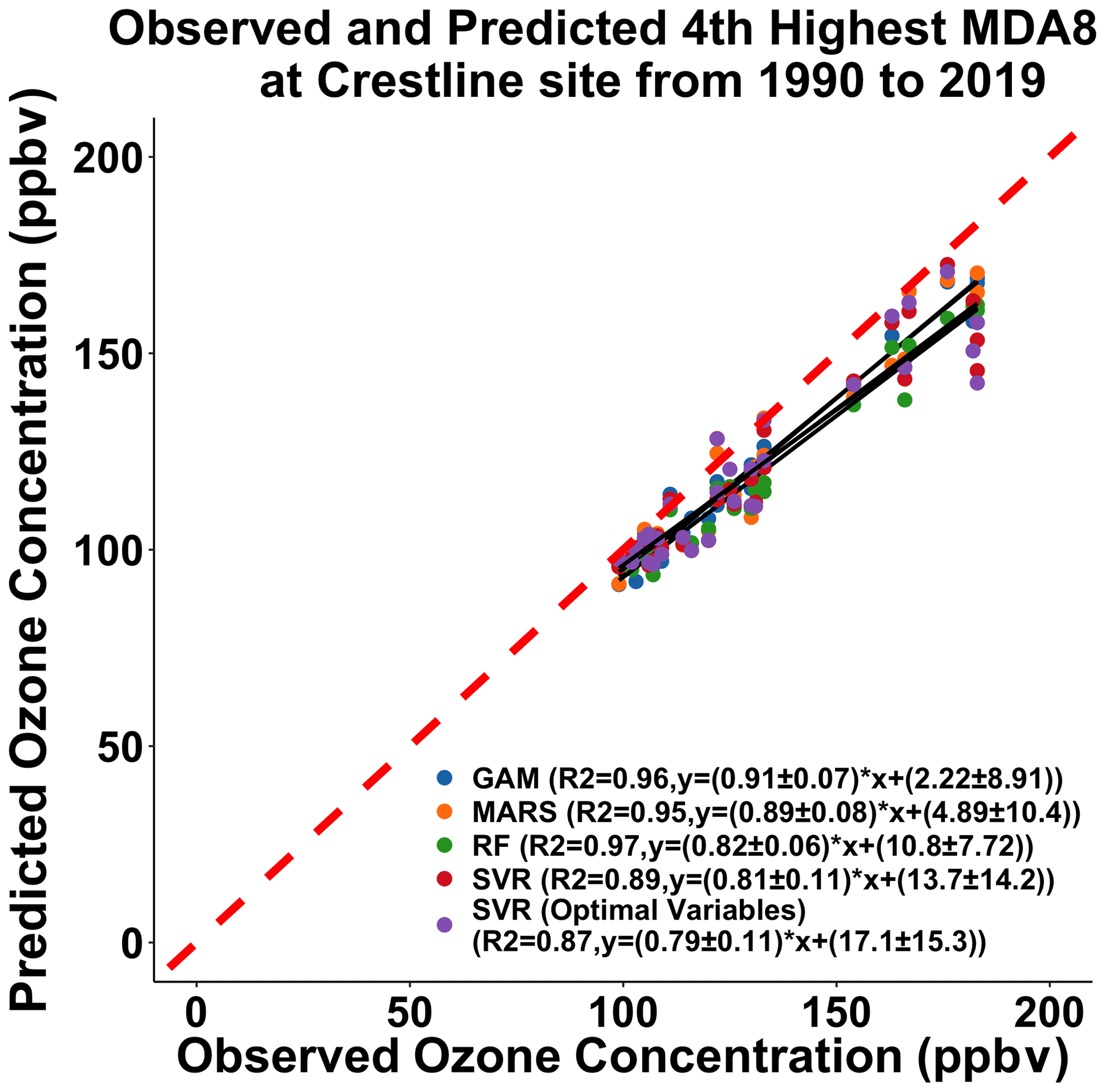
Figure 3 Comparison between the fourth highest observed and predicted MDA8 ozone concentrations using the GAM model built for the top 30 MDA8 ozone days at the Crestline site using the GAM-SoCAB-8HR V1.0 model (blue), MARS-SoCAB-8HR V1.0 model (orange), RF-SoCAB-8HR V1.0 model (green), SVR-SoCAB-8HR V1.0 model (red) and SVRoptimal-SoCAB-8HR V1.0 model (purple).

Table 1 Predictors used in the GAM and MARS model equations.

Table 2 Summary of statistical results of the fourth MDA8 ozone predictions using four methods at the Crestline site.

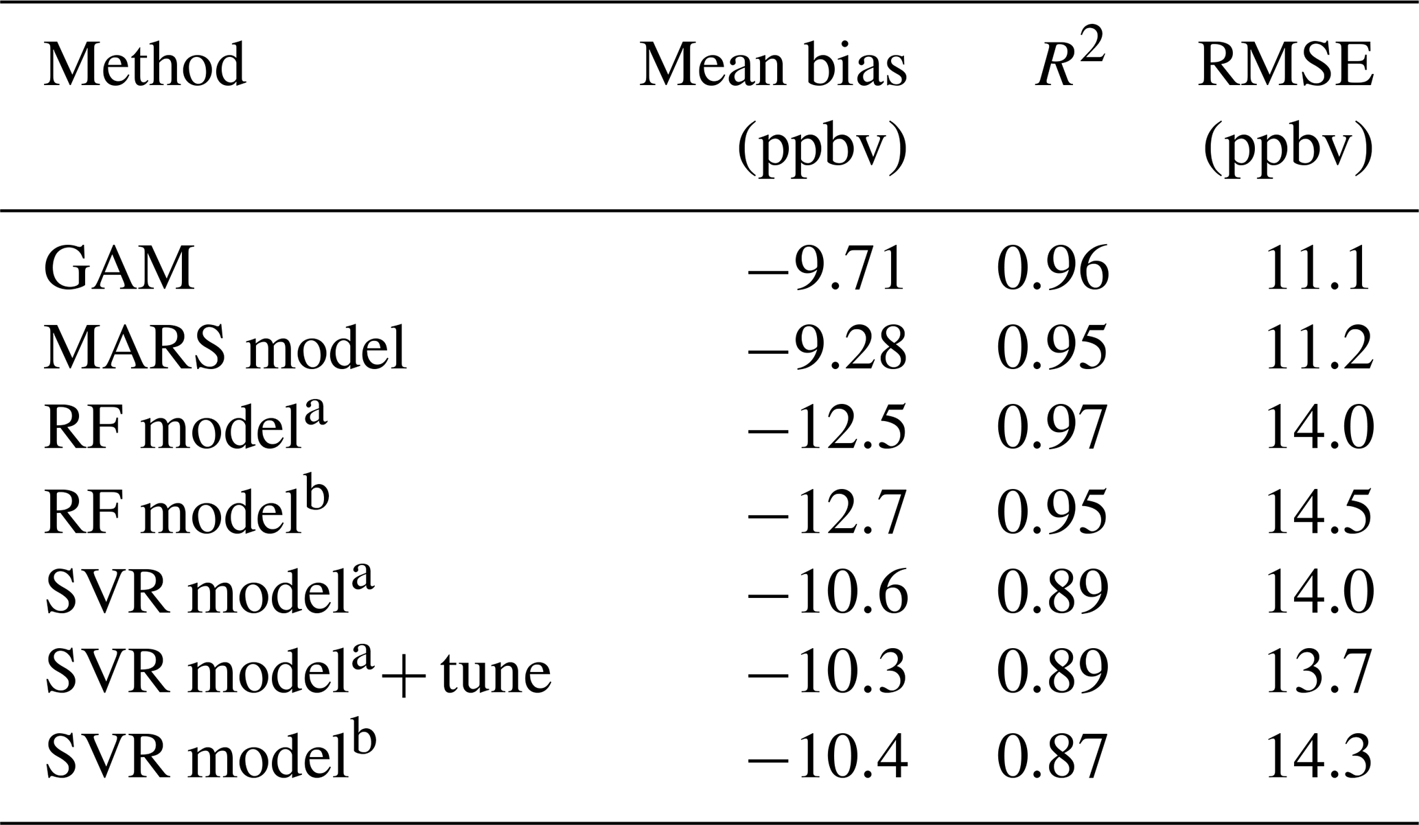
^a,b RF/SVR model with the same variables as the GAM (GAM-SoCAB-8HR V1.0) and RF/SVR model with the optimal combination of the indicators.

3.2 Comparisons among the nonlinear methods

3.2.1 Statistical results and computational time (efficiency)

We compared the R², MB and RMSE of the peak and fourth highest MDA8 ozone predictions using all these four models. The statistical results of simulations of the top 30 MDA8 ozone days showed that all these four methods explain most of the variability of observations, especially the GAM (Table S3). The GAM (GAM-SoCAB-8HR V1.0) had the lowest MB and RMSE and the highest R² for the top 30 MDA8 ozone simulations among all these four methods. Also, the GAM (GAM-SoCAB-8HR V1.0) showed the best stability of the top 30 MDA8 ozone predictions based on CV results (Table S4).

In addition, these four numerical methods can capture the fourth highest MDA8 ozone variations well. The RF model using the same variables as the built GAM (RF-SoCAB-8HR V1.0) of the fourth highest MDA8 ozone predictions with an R² of 0.97, MB of −12.53 ppbv and RMSE of 14.02 ppbv showed a lower model performance when compared to the GAM whose R² equaled 0.96, MB was −9.71 ppbv and RMSE was 11.07 ppbv. The R² for the MARS model (MARS-SoCAB-8HR V1.0) equaled 0.95 with an MB of −9.28 ppbv and RMSE of 11.16 ppbv. In comparison to the performance of the GAM, the MARS model had a better MB value but a worse R² and RMSE value. The SVR model (SVR-SoCAB-8HR V1.0) showed the highest MB and RMSE value and lowest R² among all these four methods, implying that the SVR model predictions gave the highest variations and lowest prediction accuracy. In general, all these four methods showed a similar performance to the fourth highest MDA8 ozone predictions. The predicted fourth highest MDA8 ozone levels with RF and SVR using the optimal variable combination had a lower R² and higher MB and RMSE than those using the same variables as the GAM. Therefore, the variables used in the GAM (GAM-SoCAB-8HR V1.0) were the best combination to build the models for peak ozone levels.

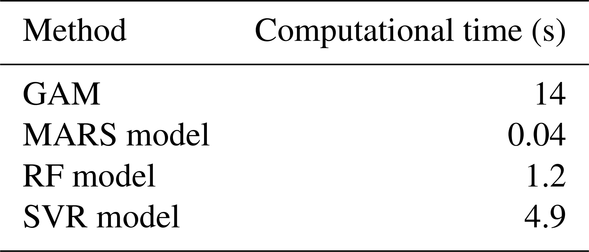
The statistical results and computational time need to be considered together to compare the model performance of all the models, especially for a large size dataset. There were no significant differences among these four methods in terms of the top 30 and the annual fourth highest ozone predictions. The GAM was marginally better compared to the other three models outside of cost effectiveness. The computational requirements for each model in this work is small due to the small dataset size (Table 3). If computational time is a key factor, the MARS model can be a good choice for a larger dataset (Table 3).

Table 3 Summary of the computational time of each model.

3.2.2 Two-step method

The R² values of the fourth highest MDA8 ozone predictions using these four regression methods were similar and agreed with the observations, but the RMSE and MB values were larger than desired. In order to reduce the bias, we applied a two-step method using the least-squares method to the fourth highest MDA8 ozone predictions. The steps are shown below:

1. Predict the top 30 MDA8 ozone concentrations from 1990 to 2019 using the models built in Sect. 3.1.

2. Extract the annual predicted fourth highest MDA8 ozone concentrations based on the date of the observations.

3. Apply the regression equation derived using the observations and the predictions in step 2 to the fourth maximum value in each year's top 30 MDA8 ozone predictions (as the response variable) to get the updated fourth highest MDA8 ozone predictions.

4. Use the regression equation from step 3 with the updated predictions to get the improved fourth highest MDA8 ozone predictions.

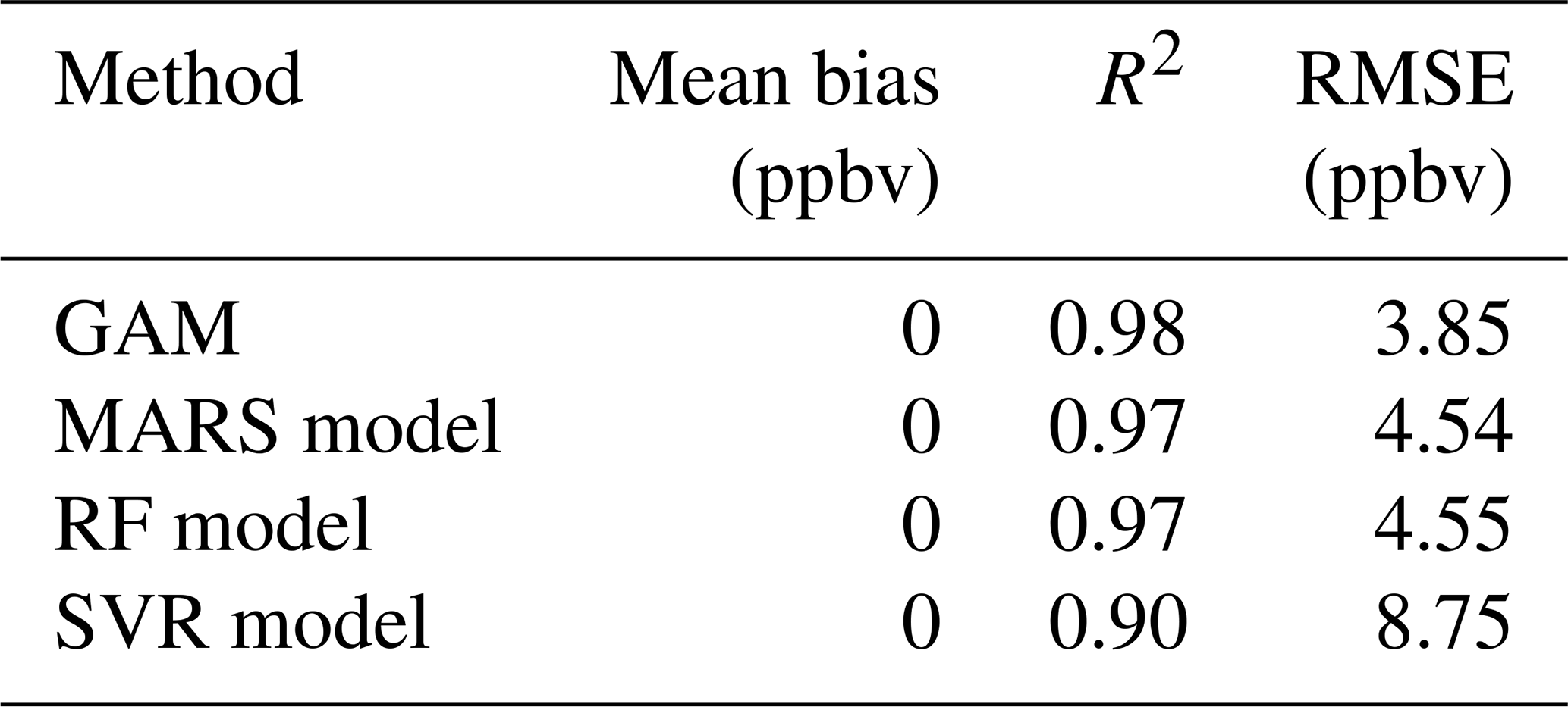
The mean bias of the improved predictions was removed; the R² value was increased; and the RMSE was reduced. After applying the two-step method, the GAM showed the best model performance among all the models with the highest R² and lowest RMSE value. The performance of the MARS model and RF model were almost the same. The improved SVR model results were still the least accurate due to the lowest R² and highest MB and RMSE.

Table 4 Summary of statistical results of the fourth MDA8 ozone predictions after applying the two-step method using four methods at the Crestline site.

3.2.3 Relative importance of the independent variables

There are multiple methods to determine the importance of each independent variable of computational models, but the differences among all the methods are negligible. The algorithms used to calculate the variable importance of the GAM, the RF model and the SVR model are similar, based on the differences between the simulations using the original dataset and the dataset with one indicator's value randomly permutated. If the change of the simulations is significant, then that indicator is important or vice versa. The variable importance shown is 1−r (r: the Pearson correlation coefficient between the simulations using the original and random-permutation datasets) when the GAM is used. The RF and SVR model used the change of mean square error between the simulations using the original and random-permutation datasets. The MARS model computed the variable importance by adding the indicator into the model and evaluating the error changes by GCV.

The precursors' emissions routinely are the most important indicators among all the variables in these four models that indicate that the emissions have more impact on the peak MDA8 ozone formation than the meteorology in the SoCAB. The maximum temperature is quite significant among all the meteorological factors. The GAM and the MARS model also included the interaction terms between the emissions and maximum temperature, which capture more variability of the peak MDA8 ozone concentrations. The maximum temperature is related to solar radiation, which has an influence on the rate of photolysis reactions. RH at 850 mb showed relatively high importance in the RF and SVR models. It had a negative correlation with peak MDA8 ozone concentrations because of its relationship with precipitation and cloud cover and, in consequence, reduced solar radiation and affected photolysis reactions.

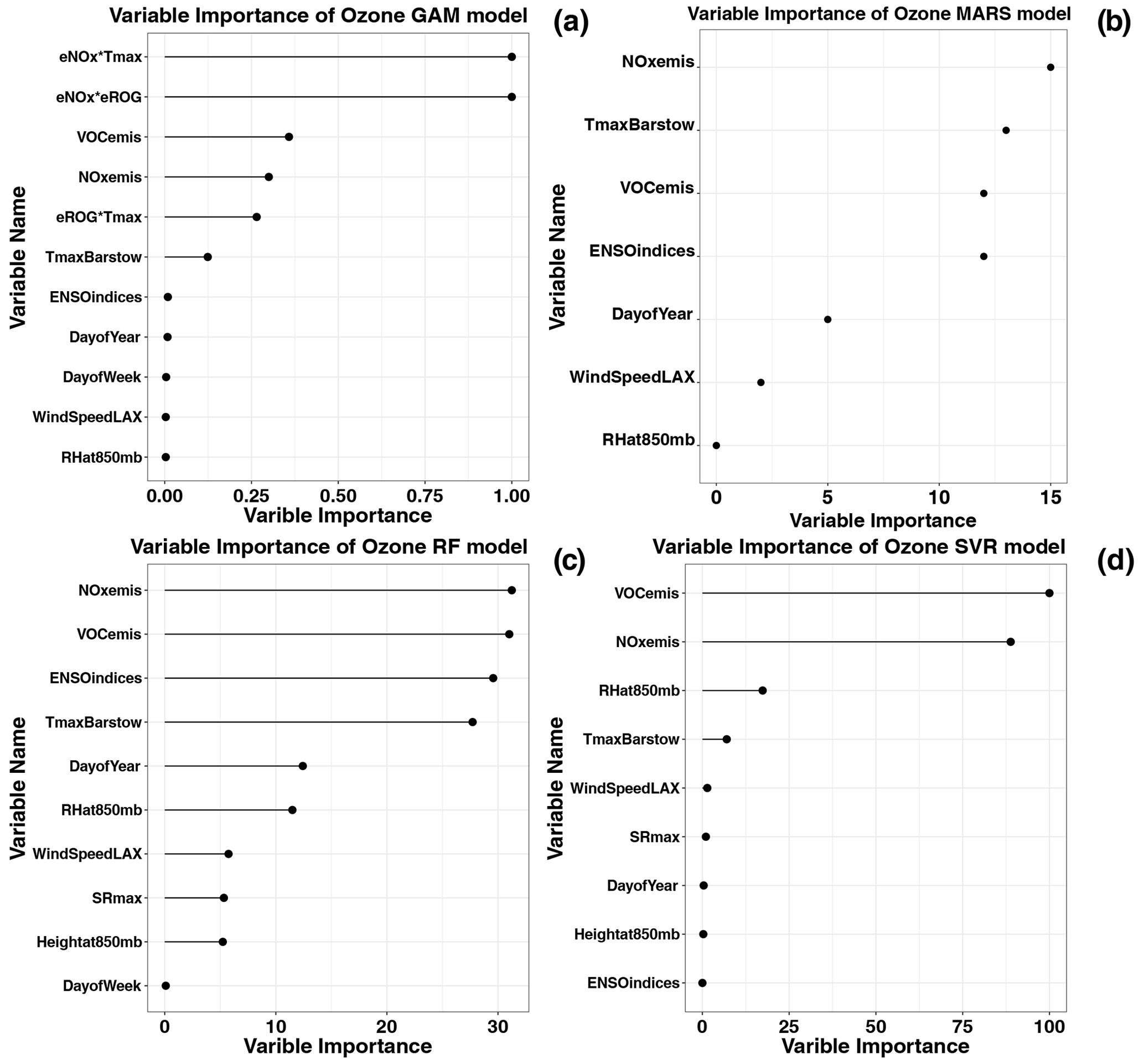
Figure 4 Variable importance for simulations of the top 30 MDA8 ozone days using the GAM-SoCAB-8HR V1.0 model (a), MARS-SoCAB-8HR V1.0 model (b), RF-SoCAB-8HR V1.0 model (c) and SVR-SoCAB-8HR V1.0 model (d). The variable importance for each model is calculated with different methods (see text). SR: solar radiation.

3.3 Limitations

There are several limitations in the comparisons among these four models. Some significant factors to the fourth highest MDA8 ozone concentrations may be excluded from the models due to the relatively small dataset that can consequently affect the prediction accuracy of the models; adding more available meteorological factors (e.g., cloud coverage, planetary boundary layer, surface wind direction and solar irradiance) and other large-scale climate indices (e.g., Atlantic Multidecadal Oscillation (AMO) and tropical Pacific sea surface temperature anomalies (TROP)), we can expect an improvement in the model performance, albeit at the cost of performance. Second, the running time of these four models with a small dataset does not show any significant differences. The computational time, however, will be a key criterion if the dataset is quite large and may affect the best model choice. Third, since we included the local meteorological variables in the model equations and the models were developed for the Crestline site, these models may not offer the same performance with the peak ozone levels at other sites in the SoCAB. Given that Crestline is downwind of Los Angeles, which then is bordered by the Pacific Ocean, the models using SoCAB emissions capture the upwind conditions. In other regions, such models could be expanded to include both local emissions and upwind states' emissions. Previous studies showed the emissions, maximum temperature, RH, wind speed, wind direction and large-scale climate patterns have impacts on the daily MDA8 ozone concentrations in different regions in the world (Blanchard et al., 2014, 2019; Camalier et al., 2007; García Nieto and Álvarez Antón, 2014; Gong et al., 2018, 2017; Jeong et al., 2020; Jin et al., 2013; Ling et al., 2013; Liu et al., 2013; Lu and Turco, 1996; Lu et al., 2019; Luna et al., 2014; Ma et al., 2020; McClure and Jaffe, 2018; Sun et al., 2019). This is similar to the variable-importance results in this study. In addition, although the GAM and MARS model outperform the RF and SVR model in this study, the machine learning methods (e.g., RF, neural network and SVR) may potentially offer better performance than the GAM and the MARS model with a significantly larger dataset. Finally, the models were not developed to predict daily MDA8 ozone concentrations because they are trained using the highest 30 MDA8 ozone levels of each year. The relationships between inputs and predicted ozone are very different at lower ozone levels.

4 Conclusions

This study compared four observation-based approaches to predict the fourth highest MDA8 ozone concentrations as a function of emissions, meteorological factors and large-scale climate patterns. The statistical results showed that these four models with estimated emissions and observed meteorological factors can explain most of the variations of the top 30 and fourth highest MDA8 ozone concentrations (R²=0.81–0.84 for the top 30 MDA8 ozone concentrations and R²=0.89–0.97 for the fourth highest MDA8 ozone concentrations). Among the top 30 MDA8 ozone models, the GAM (GAM-SoCAB-8HR V1.0) achieved the highest R² (0.84) and lowest RMSE value (9.74 ppbv), and the SVR (SVR-SoCAB-8HR V1.0) and RF (RF-SoCAB-8HR V1.0) achieved a lower R² value (0.81) and a higher RMSE value (10.9 ppbv). So, in terms of the top 30 highest MDA8 ozone predictions, there was little difference among these four models. These models showed a better performance for predicting the fourth highest MDA8 ozone predictions than the peak ozone level. All models had a high R² value (close to or higher than 0.9), but after considering RMSE and MB values, the GAM and the MARS model described the dataset better and provided a significantly better prediction accuracy as compared to the RF and SVR models. Although the computational time of each model was small for the dataset employed here, the MARS model required the least. The order of the variable importance of the factors of each model was similar. The precursors' emissions were the most significant factors for indicating the importance of the emissions impact on peak ozone levels. Maximum temperature presented relatively high importance among all the meteorological variables.