the Creative Commons Attribution 4.0 License.
the Creative Commons Attribution 4.0 License.
 | 16 Dec 2022
A method for transporting cloud-resolving model variance in a multiscale modeling framework
Walter Hannah
Kyle Pressel
An unphysical checkerboard pattern has recently been identified in the multiscale modeling framework configuration of the Energy Exascale Earth System Model (E3SM-MMF) that is hypothesized to be associated with the inability of large-scale dynamics to transport fluctuations within the embedded cloud-resolving model (CRM) on the global grid. To address this issue, a method is presented to facilitate the large-scale transport of CRM variance in E3SM-MMF. Simulation results show that the method is effective at reducing the occurrence of unphysical checkerboard patterns on a range of timescales from days to years. This result is confirmed both subjectively through visual inspection and quantitatively with a previously developed pattern categorization technique. The CRM variance transport does not significantly alter the model climate, although it does tend to reduce temporal variance on fields associated with convection on the global grid.
- Article
(2804 KB) - Full-text XML
- BibTeX
- EndNote


The multiscale modeling framework (MMF) is an innovative method to explicitly represent clouds in an atmospheric general circulation model (GCM) by coupling each GCM column to a cloud-resolving model (CRM) (Grabowski and Smolarkiewicz, 1999; Grabowski, 2001; Randall et al., 2003; Khairoutdinov et al., 2005). The two models cover vastly different scale ranges and are coupled via forcing and feedback tendencies that are formulated such that the domain mean state of the CRM cannot drift away from the state of the parent GCM column (Grabowski, 2004; Randall et al., 2016). This coupling approach leaves a “gap” in the total range of scales simulated by the coupled system where neither model can provide an explicit representation. Typically, this gap occurs at the scale of mesoscale convective systems. Despite filtering out potentially important weather systems, the scale gap can be leveraged to improve computational performance through hardware acceleration with GPUs (Hannah et al., 2020) and algorithmic CRM mean state acceleration (Jones et al., 2015).
The MMF scale gap has also been implicated in causing a “checkerboard” signal on the grid of the parent GCM by Hannah et al. (2022) in which neighboring grid cells systematically exhibit more or less convective activity. This results in a subtle, yet persistent checkerboard pattern being imprinted on the long-term mean of certain cloud-related quantities such as liquid water path and precipitation (see inset in Fig. 1b). A pattern detection method was developed to quantify the extent and persistence of the checkerboard pattern in E3SM-MMF, and a comparison with satellite data supported the intuitive conclusion that the signal was unphysical. The checkerboard detection method also revealed that Energy Exascale Earth System Model version 2 (E3SMv2) exhibits a checkerboard pattern, albeit weaker. The checkerboard signal in E3SMv2 operates through a different mechanism that is directly linked to the revised trigger for deep convection that relies on convective available potential energy (CAPE) generation by dynamics (DCAPE).
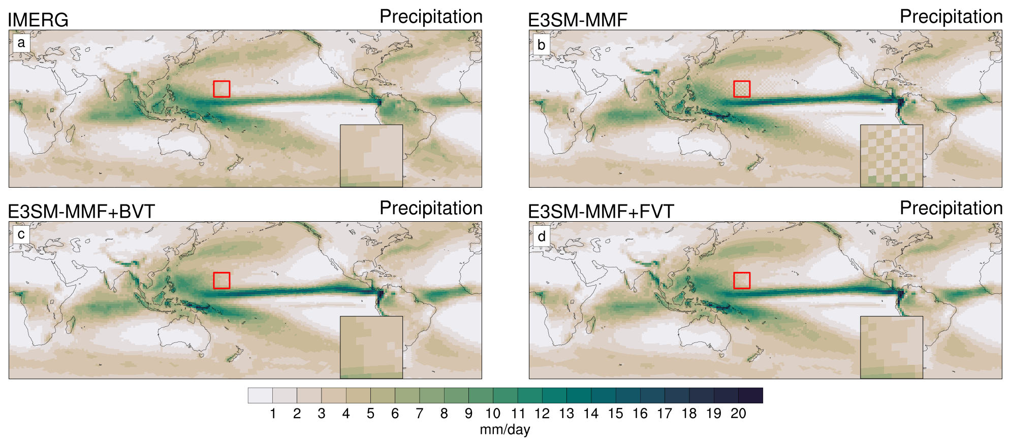
Figure 1Maps of 10-year mean precipitation for using data from Integrated Multi-satellite Retrievals for GPM (IMERG) (a), E3SM-MMF (b), E3SM-MMF with bulk variance transport (BVT, c), and E3SM-MMF with filtered variance transport (FVT, d). The red outline indicates the region shown in the inset map that highlights a region that typically has a noticeable checkerboard pattern in E3SM-MMF without variance transport.
Another consequence of the MMF scale gap is that small-scale fluctuations associated with convective circulations within the CRM cannot be advected by the large-scale flow represented by the GCM. This is because the CRM only communicates to larger scales through the coupling of the CRM domain mean (Pritchard et al., 2011). Thus, variance at the scale of convective elements can effectively become “trapped” within the CRM. This might not seem like a problematic feature of the MMF given that cloud life cycles are typically short compared to the GCM time step on the order of 10–30 min. However, the checkerboard problem in E3SM-MMF suggests that this peculiarity of the MMF approach can lead to an unphysical feedback cycle that allows the pattern to persist. Jansson et al. (2022) also explored this issue, and while they did not detect anything like the checkerboard pattern in E3SM-MMF, they showed how the lack of small-scale advection inherent to the MMF coupling strategy can lead to unnatural dissipation of a cloud field.
Another way to think about the variance trapping problem is to consider the CRM simply as a GCM parameterization of sub-grid scale (SGS) processes with a higher-order closure. The CRM is exactly solving for the GCM–SGS variance and ignoring horizontal transport which forces the system to produce a local balance between the production and dissipation of GCM–SGS variance. In the case of water vapor, a significant pathway of variance dissipation is precipitation, but because precipitation can only dry the system, it leads to an anomalous effect on the CRM mean, which can in fact be transported, and sets up the checkerboard.
An ideal solution to this issue is to allow the CRM fluctuations to be advected by the flow of the large-scale model, since this interaction between scales happens naturally in the real atmosphere. The quasi-3D framework of Jung and Arakawa (2014) is one way to enable this type of scale interaction, but this method is still in an experimental phase and not well suited to being implemented into the current E3SM infrastructure. Another potential solution that has been proposed in our discussions is to relax the requirement of cyclic horizontal boundary conditions in the CRM. Several versions of how this could be achieved have been discussed and we have conducted experiments with one approach (not shown), but all of these involve problematic compromises that discourage a detailed exploration.
The most tractable solution for transporting CRM fluctuations, or variance, is to encode these fluctuations into a set of massless tracer fields that can be advected by the large-scale dynamics. Developing this method requires defining how the variance will be encoded, as well as how the variance tracers on the GCM grid will be coupled to the actual variance within the CRMs. In this study we present such a method for transporting cloud-scale variance in E3SM-MMF. The general variance transport method is detailed in Sect. 2 along with a discussion of possible variations on the method. This is followed by a description of model experiments, satellite data, and checkerboard detection method used to validate the variance transport in Sect. 3. Discussion of the results and conclusions are presented in Sects. 4 and 5.
2.1 MMF coupling review
The canonical MMF coupling involves forcing and feedback tendencies of some quantity q between a large-scale model (GCM) and small-scale model (CRM, Grabowski, 2004). The values of q are defined independently for each model, but the tendencies must be formulated such that the q fields of each model maintain equality at the end of each time step. This coupling procedure starts with a provisional time step where the GCM updates the GCM variable denoted qG with a tendency BG which includes things like advection over the GCM time step ΔtG. So we write
so that
The tilde denotes a provisional value, and Eq. (1) represents a partial time step. The corresponding CRM variable qC is updated using the CRM time step ΔtC:
The subscripts m and m+1 denote successive CRM time steps. The term BC represents the processes calculated within the CRM, such as microphysics. The quantity is the CRM domain average of qC at the beginning of the GCM time step. The last term of Eq. (3) is the mechanism that communicates the tendencies of the GCM to the CRM. In other words, it is the forcing of the CRM by the GCM.
After taking enough CRM time steps to span the length of the GCM time step, the GCM variables are updated with a feedback tendency:
Here represents the horizontal mean qC at the end of the CRM integration or at GCM time n+1.
Comparing the two sides of Eq. (6), we see that
which indicates that the two model states are identical at the end of the GCM time step, or, equivalently, at the beginning, and guarantees that the two model states cannot drift apart.
2.2 CRM variance coupling
To implement the coupling of variance between CRMs in the MMF we can largely follow the coupling scheme for an arbitrary tracer as described above. However, since we are only concerned with fluctuations about the CRM mean state, we do not want the forcing tendencies to have any impact on the CRM mean state. Thus, the CRM forcing must only operate on local perturbations from the horizontal mean. For coupling back to the GCM we use a bulk measure of the variance within the CRM to provide feedback tendencies to a set of massless variance tracers advected on the global grid. The GCM variance tracers are only used to move the CRM variance around, analogous to how clouds and small-scale turbulence can be advected by large-scale flows in the real world.
The CRM variance feedback tendency of some quantity q at a given vertical level of the CRM that is applied to the GCM can be formulated analogous to Eq. (4):
where Q represents the massless variance tracer on the GCM grid and q′ is the perturbation from the horizontal mean on the CRM grid. The quantity is the total variance of q at the end of the CRM time integration.
Since the CRM columns do not have any specific location within the parent GCM column, the forcing or “injection” of variance into the CRM cannot be constrained to any particular spatial pattern. Thus, we rely on scaling the existing perturbations from the horizontal mean at each time step so that the existing spatial structure of variance within the CRM is preserved. To do this we calculate a scaling factor α at each CRM time step to scale the existing perturbations and increase or decrease the existing variance to be consistent with the variance forcing.
In order to constrain the scaling factor α, the total variance forcing applied to the CRM can be formulated analogous to Eq. (3):
so that
Note that we are ignoring the internal CRM processes that will affect the variance, but this is not important for formulating α.
At each time step the adjusted variance can be formulated in terms of the variance of the scaled perturbations or by scaling the total variance by α2:
By combining Eqs. (9) and (10) we can solve for α as
where represents the variance forcing provided by the GCM (i.e., advective tendencies).
In practice, the variance forcing is applied at each CRM time step by calculating the perturbations of q from the horizontal mean and the corresponding value of α at each vertical level. The existing q perturbations are then scaled by α and converted into a tendency to be applied back to the full state. This allows alternate definitions of the perturbations such that the variance transport can be restricted to a certain scale range (see discussion below). In certain rare circumstances the variance forcing can be too strong and lead to instability within the CRM. Since we are not concerned about preserving the cloud-scale variance of thermodynamic tracers globally, we can address this issue with a simple limiter. We find that restricting α between 0.90 and 1.10 works well for these edge cases and does not qualitatively affect the model behavior (not shown).
Another important step for implementing the variance transport method is to decide which quantities will be affected. Currently, the CRM in E3SM-MMF uses liquid–ice static energy and total non-precipitating water as the main prognostic thermodynamic quantities. These are the only two thermodynamic quantities directly affected by variance transport in E3SM-MMF. Note that the variance transport does not affect the mean state of the CRM and, thus, does not affect energy or mass conservation. The single-moment microphysics scheme employed by the CRM allows cloud liquid and ice to be diagnosed from the total water, so there is no need to consider the variance of cloud condensate. We initially avoided transporting variance of the horizontal momentum field due to concerns about complications arising from the use of the anelastic approximation. However, we have since enabled momentum variance transport and found that it results in a notable contribution to suppressing the checkerboard pattern (not shown), so the simulations discussed here include horizontal momentum variance transport.
2.3 Alternative approaches
Jansson et al. (2022) used a different approach to facilitate variance transport in which only total water anomalies were scaled to force the CRM cloud water to match the corresponding fields of the parent model. They showed that this approach effectively allows the spatial variability of the cloud field to be advected between columns of the parent model, but they also reported a curious problem where the cloud water added by their scaling was rapidly dissipated over the course of the CRM integration. We are interested in comparing these methods and the dissipation issue, but this is outside the scope of the current study. Also, E3SM-MMF currently lacks the infrastructure to output CRM data at the frequency of the CRM time step which limits our ability to directly compare their results.
We refer to the variance transport method described above as “bulk variance transport”, since we lump the CRM fluctuations of all scales together by calculating the total variance at each vertical level. The bulk approach makes no distinction as to what scales are most represented in the variance tracers and because we rely on the existing perturbations in a CRM when applying the variance forcing, it is possible to transport relatively large-scale variance in one CRM and inject it into the smallest scales of another CRM. During the course of this work we have considered a few alternative approaches to address this inter-scale variance transport that allow for some flexibility in choosing which scales are represented in the variance that is being transported.
One of the earlier ideas was to transport multiple scalars for each prognostic CRM variable corresponding to the Fourier transform coefficients obtained from the horizontal dimension. This idea was appealing because it allowed the variance at each scale to be transported separately, so there was no chance of inter-scale variance exchange. However, experiments with this approach were much less effective at reducing the checkerboard pattern occurrence. We suspect this method is fundamentally flawed because it ignores the important cancellations between Fourier modes that give rise to a realistic atmospheric state. It is also a more expensive method due to the larger number of tracers.
Another alternative that we have explored is to use a low-pass spatial filter to isolate a certain scale range for the perturbations used to define the variance tracers. By using a filtered CRM state we can restrict the inter-scale variance exchange to occur only within the bounds defined by the filter. In our experiments we use a fast Fourier transform (FFT) to serve as a low-pass filter in the horizontal dimension of the CRM to isolate the largest few wavenumbers. The resulting filtered perturbations can be used in the method for variance forcing and feedback calculations outlined above without modification. Experiments using this filtered variance transport technique were consistent with the bulk variance transport experiments, with some subtle, but unique, changes to certain climatological features. Further sensitivity experiments show that the filtered method converges to the bulk method as the cutoff wavenumber is increased (not shown). Ultimately, our analysis suggests that the potential inter-scale variance transport is not problematic, so it is preferable to use the bulk method, but we have included a case with the filtered method in our analysis below.
3.1 Checkerboard detection method
For a quantitative assessment of the checkerboard pattern we use the pattern detection method developed by Hannah et al. (2022), which is briefly described here. After several attempts to automate the detection of a “pure” checkerboard pattern with alternating anomalies over a large area, it became clear that pure checkerboard instances are rare on short timescales. More often the data show a “partial” checkerboard due to the coexistence with a synoptic-scale gradient. Hence, a detection method to study the checkerboard issue is needed to be able to distinguish various partial checkerboard patterns.
To overcome this partial checkerboard complication Hannah et al. (2022), limited the scope of the problem to only consider the eight locally adjacent neighboring grid cells surrounding a given cell (i.e., the neighbors sharing an edge or corner) and encoded the adjacent values as 0 for values less than or equal to the central value and 1 otherwise. These neighborhood values are ordered clockwise around the central point, starting with the northernmost edge neighbor for consistency. Points located adjacent to the cube sphere corners are omitted, since they only have seven adjacent neighbors. The resulting sequence of eight binary values (ignoring the center cell) for a given location and time represents 1 of 36 possible unique patterns after considering that certain sets of patterns are identical when rotated (i.e., rotational symmetry). The goal of this pattern detection method is to catalogue the occurrence of each unique pattern and compare it to satellite data to determine if any patterns are occurring too frequently (see Hannah et al., 2022 for more details).
Using this method, a pure checkerboard pattern shows up as an alternating sequence of 1s and 0s. This pattern is relatively rare when considering daily mean data, which are what we use to facilitate the comparison with satellite data. The rarity of the pure checkerboard is somewhat expected due to ubiquitous synoptic-scale gradients that can coexist with the pure checkerboard on short timescales. There is no clear way to separate these synoptic signals from the underlying checkerboard, so it is useful to focus on patterns that contain only a portion of the full checkerboard pattern. To do this we further identify which of the 36 patterns contain a continuously alternating binary sequence of length four or more and consider these to be partial checkerboard patterns. Alternate definitions of partial checkerboard patterns were not found to qualitatively change our results (not shown).
3.2 E3SM-MMF description
E3SM was originally forked from the NCAR Community Earth System Model (CESM) (Hurrell et al., 2013) but has undergone significant development since then (Golaz et al., 2019; Xie et al., 2018). The dynamical core uses a spectral element method on a cubed-sphere geometry (Ronchi et al., 1996; Taylor et al., 2007). Physics calculations are done on a finite volume grid that is slightly coarser than the dynamics grid but matches the effective resolution of the dynamics grid more closely (Hannah et al., 2021).
The MMF configuration of E3SM (E3SM-MMF) was originally adapted from the super-parameterized Community Atmosphere Model (CAM) (SP-CAM; Khairoutdinov et al., 2005). E3SM-MMF has also undergone significant development, but the model qualitatively reproduces the general results published in previous studies (Hannah et al., 2020). The embedded CRM in E3SM-MMF is adapted from the System for Atmospheric Modeling (SAM) (Khairoutdinov and Randall, 2003). Microphysical processes are parameterized with a single-moment scheme, and sub-grid-scale turbulent fluxes are parameterized using a diagnostic Smagorinsky-type closure. Aerosol concentrations are prescribed with present-day values. Convective momentum transport in the 2D CRM is handled using the scalar momentum tracer approach of Tulich (2015).
The embedded CRM in E3SM-MMF uses a two-dimensional domain with 64 CRM columns in a north–south orientation and 2 km horizontal grid spacing. The global model uses a hybrid vertical coordinate that transitions from terrain following near the surface to a pure pressure coordinate near the top. The CRM employs the anelastic approximation and uses a height vertical coordinate. The mismatch in vertical coordinates turns out to be inconsequential for the MMF coupling scheme because the CRM background pressure and density can be updated with profiles from the GCM at each coupling step without causing an unphysical shock to the system.
In order to facilitate better CRM performance when running on GPU machines, the CRM was completely rewritten in C++ (SAM++), which provides substantially improved GPU throughput over the original Fortran code with OpenACC directives. The SAM++ model relies on the performance portability library of Yet Another Kernel Launcher (YAKL). 1 In addition to GPU hardware acceleration, E3SM-MMF can also leverage algorithmic acceleration through the mean-state-acceleration scheme of Jones et al. (2015). Additional refactoring of the MMF physics code enabled the enhancement of the hardware acceleration by minimizing data transfer overheads between CPU and GPU, as well as leverage OpenMP threading to maximize the throughput of calculations outside of the CRM.
E3SM-MMF uses a simple technique to reduce the number of radiative transfer calculations in order to boost throughput. Rather than performing radiation calculations on each CRM column separately, these calculations are performed on the average state of 4 groups of 16 adjacent CRM columns and the resulting radiative tendencies are applied homogeneously back to the same group of columns (Hannah et al., 2020). This provides a significant boost to the throughput without qualitatively affecting the general characteristics of radiative fluxes (not shown). A forthcoming paper will provide a detailed exploration of the model's sensitivity to how these radiative groups are configured.
Aside from the difference in how convection is treated, E3SM-MMF differs from the standard configurations of E3SM in several important ways. The stability of E3SM-MMF is noticeably improved by reducing the global model's physics time step from 30 to 20 min. The 72-layer vertical grid of E3SMv2 was also found to be problematic for the performance of E3SM-MMF because thin layers near the surface necessitate a 5 s CRM time step for numerical stability. Therefore, the E3SM-MMF simulation shown here uses an alternative 60-layer vertical grid that allows a longer 10 s CRM time step. A final stability concern has to do with high-frequency oscillations of temperature, humidity, and wind near the surface. Both models exhibit these oscillations, but they render E3SM-MMF much more susceptible to crashing. A temporal smoothing of surface fluxes with a 2 h timescale is used to address this problem, which does not have any notable impact on the model climate (not shown).
3.3 E3SM-MMF simulations
All simulations are run for 10 years using 128 nodes of the Oak Ridge Leadership Computing Facility (OCLF) Summit machine (768 ranks). The global cubed-sphere grid was set at ne30pg2 (30 × 30 spectral elements per cube face and 2 × 2 FV physics cells per element), which roughly corresponds to an effective grid spacing of 150 km, while the average spacing of spectral nodes for dynamics is closer to 100 km. The model input data for quantities such as solar forcing, aerosol concentrations, and land surface types are derived from a 10-year climatology between 2005–2015 to be representative of climatological conditions around 2010. Sea surface temperatures were similarly prescribed using monthly climatological values that are temporally interpolated to give a smooth evolution (Taylor et al., 2000).
3.4 Satellite observation data
Following Hannah et al. (2022), we use the same pattern detection method to assess the occurrence of checkerboard patterns in E3SM-MMF. We will also use satellite data that have been remapped to the model grid to serve as a benchmark for how much noise should be tolerated in the model data. The specific time period of satellite data used for analysis is arbitrary. We choose to use daily mean data between 2005–2014 for all datasets. Since the checkerboard pattern is most visible in cloud liquid water path and precipitation fields, we use comparable satellite estimates of these fields to provide a baseline of the spatial distribution of these quantities.
Satellite estimates of cloud liquid water path are provided by the Multisensor Advanced Climatology of Liquid Water Path (MAC-LWP) data product (Elsaesser et al., 2017). We use a daily-resolution version of the product (McCoy et al., 2020) with LWP estimates provided on a 1.0∘ × 1.0∘ equiangular grid that is then regridded to the ne30pg2 grid used by the model. MAC-LWP additionally provides total (cloud plus precipitating) liquid water path estimates (TLWP), and we use TLWP to create a gridded quality control mask that hashes regions for which the ratio of LWP to TLWP is less than 0.6, broadly following the recommendation of Elsaesser et al. (2017). Hashed regions envelope grid boxes for which LWP estimates exhibit substantial uncertainty (and potential systematic bias) due to errors in isolating and quantifying the cloud liquid water radiometric signature from that of the total liquid water radiometric signature in microwave retrievals.
The Global Precipitation Measurement (GPM) mission, the successor to the Tropical Rainfall Measuring Mission (TRMM), was launched in 2014 with the goal of producing accurate and reliable estimates of global precipitation with all available TRMM and GPM data eras (Hou et al., 2014). The Integrated Multi-satellite Retrievals for GPM (IMERG) combines several satellite datasets to produce an integrated rainfall data product that has proven to perform well in various regions (Anjum et al., 2018; Kim et al., 2017). Daily mean IMERG data are available on a 0.1∘ × 0.1∘ grid, which is much finer than the grid used here for the model simulations. To facilitate direct comparison we regrid the IMERG data to the ne30pg2 model grid and a 1.0∘ × 1.0∘ equiangular grid to match the MAC-LWP data.
Note that the act of data regridding does indeed affect the results of our checkerboard detection method. This was explored in more detail by Hannah et al. (2022), and the results showed a small impact that did not affect the conclusions. It is important to put the observational data on the model grid in this case in order to determine the level of naturally occurring noise that should be expected at the scale of the model grid.
In addition to our checkerboard analysis and mean-state assessment, we are also interested in characterizing any change in modes of variability that might occur from enabling variance transport. For this we will focus on analyzing tropical wave variability and will use daily mean outgoing longwave radiation (OLR) from the National Oceanic and Atmospheric Administration (NOAA) polar-orbiting satellites (Liebmann and Smith, 1996) as our observational benchmark.
In this section we will compare E3SM-MMF results from simulations that employ the bulk variance transport (BVT) and filtered variance transport (FVT) methods described in Sect. 2 to a control simulation of E3SM-MMF with no variance transport and satellite data.
4.1 Climatology
Figure 1 shows 10-year mean maps of precipitation from IMERG and model data on the model's ne30pg2 physics grid using shaded polygons to highlight signals at the grid scale. All simulations exhibit a similar spatial distribution of precipitation with typical biases relative to observations, such as too little precipitation over the Amazon, too much precipitation over the northwestern tropical Pacific and Pacific Inter-Tropical Convergence Zone (ITCZ), and a prominent double ITCZ.
The control simulation produces a noticeable checkerboard pattern, particularly in subtropical regions, consistent with the results of Hannah et al. (2022). Similar results can be found for other variables related to convection (not shown). Both BVT and FVT simulations have a smoother climatology with no clear checkerboard patterns in the long-term mean while still retaining the characteristic spatial distribution. This confirms that the variance transport method is able to address the variance trapping issue that we hypothesize is producing checkerboard patterns in E3SM-MMF.
Climatological differences of precipitation and liquid water path relative to the control simulations reveal that changes induced by variance transport are not restricted to reducing the checkerboard signal (Fig. 2). Regional changes in convective activity include a slight enhancement of precipitation in the northwestern tropical Pacific, where there is often too much precipitation in MMF models (Khairoutdinov et al., 2005). Overall, the magnitude of climatological changes from variance transport seems relatively small, such that the net top-of-atmosphere radiative balance in these simulations differs by less than 1 W m−2 (not shown). Thus, we conclude that enabling variance transport does not significantly alter the model climate.
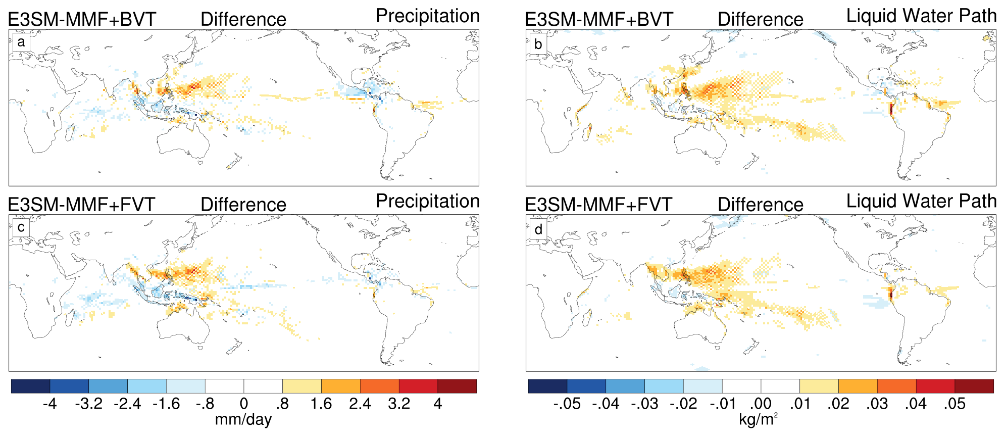
Figure 2Maps of 10-year mean precipitation and liquid water path differences relative to the E3SM-MMF control simulations for E3SM-MMF+BVT (a, b) and E3SM-MMF+FVT (c, d).
4.2 Checkerboard noise
The pattern detection method described in Sect. 3.1 yields 36 unique binary sequences that can be catalogued across specific regions and time periods and normalized by the total number of valid observations to give a “fractional occurrence” for each pattern or set of patterns. Considering the number of “valid” observations is especially important for the satellite data because it includes instances of missing data. In order to further condense these statistics we can estimate the “smoothness” of each unique pattern by counting the number of local extrema in the binary sequence. A local extreme is identified as either a 1 surrounded by 0 values or vice versa. The smoothness of a pattern can then be inferred from the number of local extrema.
Figures 3a and c show the fractional occurrence of the various unique neighborhood state patterns of liquid water path and precipitation data from the northwestern tropical Pacific after combining them based on the number of local extrema. The difference of each fractional occurrence value relative to the corresponding satellite data on the ne30pg2 grid is shown in Fig. 3b, c. This analysis highlights how the pure checkerboard (eight local extrema) is quite rare, and this pattern is observed too often in the control simulation (red bars). The control simulation has an even larger prevalence of patterns with three, four, and five local extrema relative to all other datasets owing to the fact that instances of partial checkerboard are more prevalent than instances of pure checkerboard in daily mean data. Inversely, the smoothest patterns with no local extrema are produced too infrequently in the control. Both BVT (green) and FVT (blue) cases are more similar to satellite observations in their distribution of pattern occurrence, with the BVT case being the most similar to observations.

Figure 3(a, c) Fractional occurrence of neighborhood patterns combined according to the number of local extrema (see text) over the region 0–30∘ N and 140–220∘ E (see inset map) for 10 years of satellite and E3SM-MMF data. Results for IMERG precipitation and MAC liquid water path were calculated from data regridded to the ne30pg2 grid used by the model for direct comparison. (b, d) Difference of fractional occurrence relative to satellite data.
Figure 4 shows a map of partial checkerboard fractional occurrence using liquid water path data, which is calculated by averaging the partial checkerboard occurrence after running the detection algorithm on daily mean data. The spatial distribution of partial checkerboard occurrence is similar among all three simulations, but the BVT and FVT cases show a dramatic reduction in how often these patterns are observed. However, these cases are still producing more checkerboard instances compared to satellite data, consistent with Fig. 3.
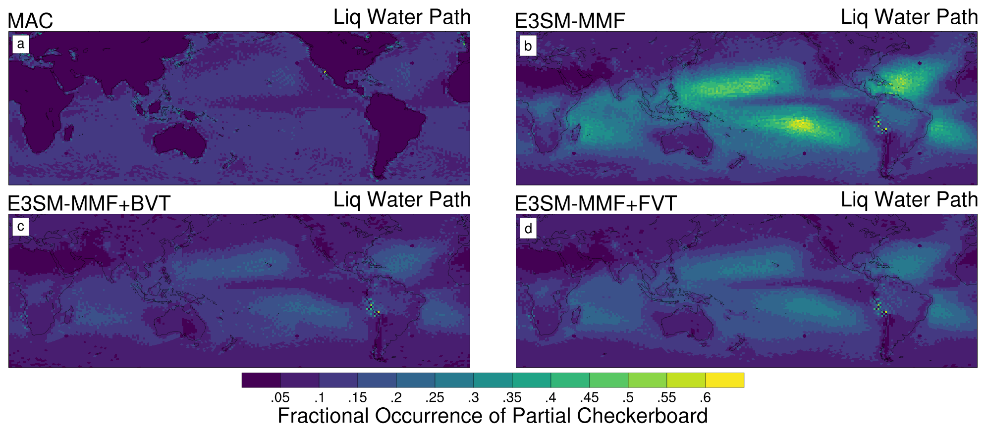
Figure 4Maps of fractional occurrence of partial checkerboard patterns (see text) on the ne30pg2 grid for MAC-LWP (a), E3SM-MMF (b), E3SM-MMF with bulk variance transport (BVT, c), and E3SM-MMF with filtered variance transport (FVT, d).
In addition to showing the more frequent occurrence of checkerboard patterns, Hannah et al. (2022) also found that checkerboard “events” were surprisingly persistent by identifying periods in which a neighborhood stays in a partial checkerboard state for an extended time period. Figure 5 shows a histogram of these partial checkerboard event lengths in liquid water path and precipitation fields using oceanic data between 60∘ S–60∘ N. In both variables we see that E3SM-MMF shows a larger number of events of any length when compared to satellite data, with some events lasting nearly 100 d. The FVT case also exhibits a tendency to produce longer partial checkerboard events than is observed in satellite data, whereas the BVT case is very similar to the satellite data.
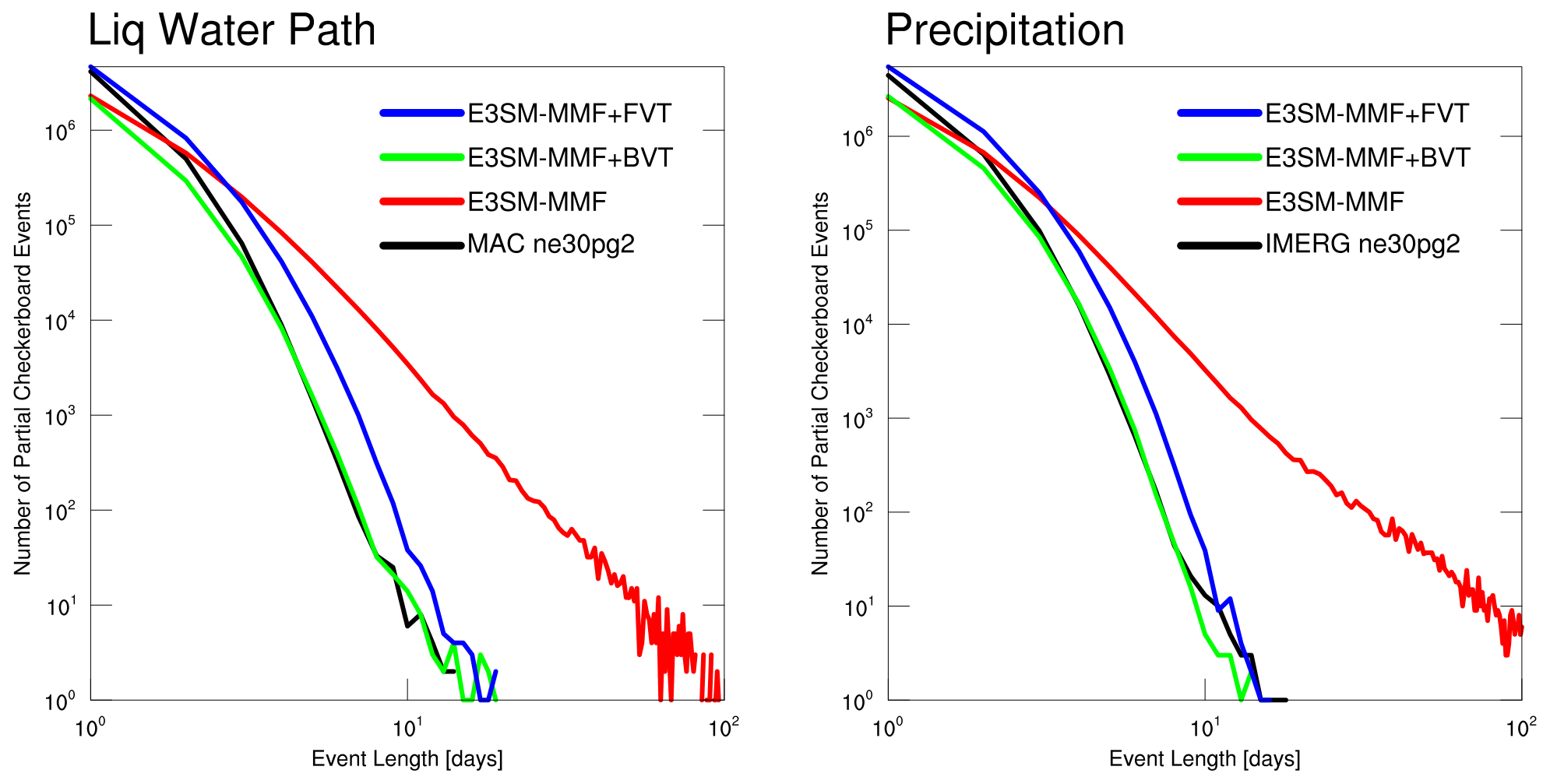
Figure 5Histogram of the event length, with events defined as continuous periods with partial checkerboard neighborhood states. Data were restricted to oceanic points equatorward of 60∘ latitude in both hemispheres for all 5 years available.
The use of daily mean data for pattern detection in the previous analysis was meant to facilitate the comparison with satellite data, but it is insightful to consider finer timescales in order to see how the checkerboard patterns “spin up” at the start of a simulation. To investigate this question we reran E3SM-MMF for 10 d with output at every time step (20 min) and ran each snapshot through our detection algorithm. Figure 6 shows a time series of the fractional occurrence of partial checkerboard patterns at each model time step from the beginning of each simulation. Data are restricted to ocean regions between 60∘ S–60∘ N, and the horizontal black dashed lines indicate the climatological fractional occurrence of partial checkerboard patterns from the corresponding satellite data for reference. Interestingly, the checkerboard signals are detectable in the first few time steps for liquid water path but are slower to spin up in the precipitation field. After the initial spin-up the occurrence of partial checkerboard patterns continues to increase over the first 4–5 d before leveling off. The speed of the initial spin-up is consistent with the authors' experience that convection within the CRM develops very quickly after initialization. This further illustrates that while the CRM variance transport method can ameliorate the checkerboard pattern persistence and yield a much smoother climate, the model still produces a relatively noisy solution on short timescales relative to satellite observations.

Figure 6Time series of partial checkerboard occurrence calculated at each model time step from the start of the run. Data were restricted to oceanic points equatorward of 60∘ latitude in both hemispheres.
4.3 Variance tracer analysis
In this section we look at the CRM variance tracers directly. We characterize the climatological distribution and how they are related to precipitation as a measure of convective activity. We also examine the GCM-to-CRM forcing and CRM-to-GCM feedback tendencies that are used to couple the two models in order to explore how CRM variance is produced and transported. This discussion is meant to provide a broad sense of how the CRM variance transport works in practice.
Figure 7 shows the zonal mean climatology of all three CRM variance tracer amounts on the GCM grid (left) along with the CRM feedback (middle) and GCM forcing (right) tendencies. For this analysis we only use data from the BVT case as the control does not have these quantities and results from the FVT case are effectively identical. The largest CRM variance tracer magnitudes occur in the tropics, which is expected, since this is where the strongest convective activity occurs. There is also a noticeable amount of CRM variance around the upper tropospheric jet regions, which is likely associated with mid-latitude storm activity. We do not have an appropriate dataset with which to compare the magnitude of the CRM variance, but using a global cloud-resolving model for this sort of comparison might be an insightful avenue for future refinement of the variance transport method.
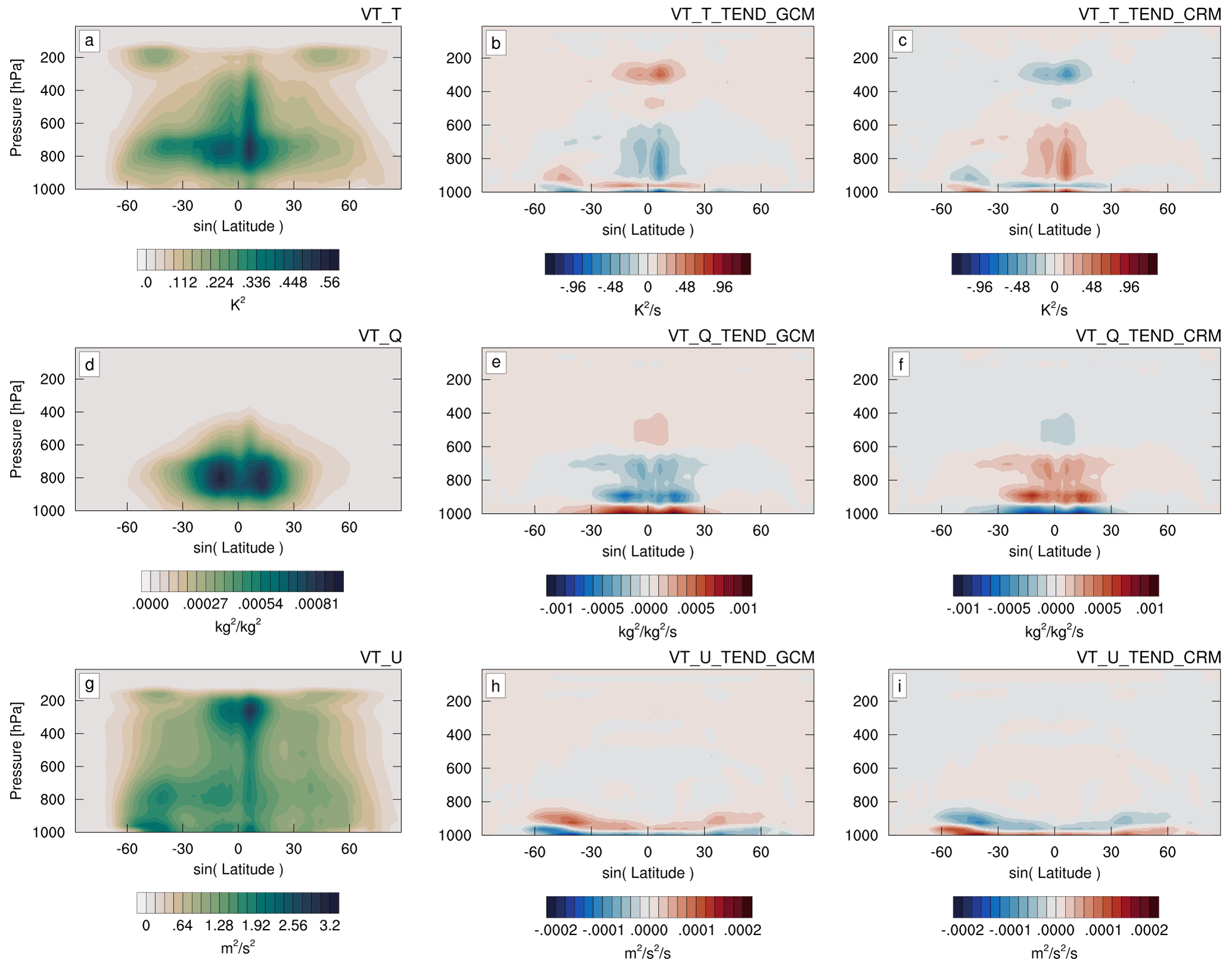
Figure 710-year zonal and time-averaged CRM variance transport tracer amount (a, d, g), GCM to CRM forcing tendency (b, e, h), and CRM to GCM feedback tendency (c, f, i) for the E3SM-MMF+BVT case. These variance amounts and tendency values correspond to the variance transport of liquid–ice static energy (a, b, c), total non-precipitating water (d, e, f), and horizontal momentum (g, h, i).

Figure 8Vertical profiles of CRM variance transport tracer amount (left), CRM feedback (middle), and GCM forcing (right) binned by precipitation rate for liquid–ice static energy (top row) and total water (bottom row) using 1 year's daily mean data from the E3SM-MMF+BVT case.
The GCM forcing and CRM feedback tendencies are expected to balance each other. This is similar to any quantity that is coupled across the two models using the MMF coupling scheme described in Sect. 2.1, and this balance is a reflection of the way the scheme is designed to not allow the state of either model to drift away from the other. However, some aspects of the zonal mean tendency structures are not immediately intuitive to understand. We might naively expect the CRM to produce positive variance tracer tendencies on average as a result of the conversion of available potential energy that drives turbulence and convection, which would be balanced by negative tendencies from the advection by the GCM, but this does not seem to be the case.
The general vertical distribution of forcing and feedback tendencies also reveals a complicated picture, with the CRM producing negative feedback tendencies at low levels and above 500 hPa. Part of the explanation may be that CRM variance produced in the boundary layer is often advected upwards into the free troposphere, leading to an apparent low-level sink of CRM variance. A full explanation of these tendencies would require a detailed budget calculation to quantify how variance is produced and transported in both the CRM and GCM, which is outside the scope of the present study.
An alternative way to examine the CRM variance tracers is to bin daily mean data by the daily mean precipitation rate to get a sense of how the feedback and forcing tendencies balance across various convective regimes. This analysis is shown in Fig. 8 using 1 year of data from the BVT case. This approach reveals a more consistent picture of how the CRM variance tracer forcing and feedback tendencies are balanced. The CRM tendency of liquid–ice static energy is positive on average when precipitation is being produced, consistent with our expectations. The CRM tendency of total water variance shows strong negative values aloft that get stronger with higher precipitation rates. These negative tendencies are likely explained by the fact that precipitation is generally a sink of total water variance.
4.4 Does variance transport affect variability?
In this section we provide a cursory look at how the CRM variance transport affects variability by focusing on convectively coupled waves in the equatorial region. Figures 9a–d show unnormalized symmetric spectra of top-of-atmosphere outgoing longwave radiation (OLR) over the region 15∘ S–15∘ N for NOAA satellite observations, E3SM-MMF, E3SM-MMF+BVT, and E3SM-MMF+FVT following Wheeler and Kiladis (1999). Lower panels (e)–(f) show the difference between each simulation relative to NOAA observations. Positive and negative wavenumbers indicate eastward and westward propagating modes, respectively. Theoretical dispersion lines are shown for equatorial Kelvin and Rossby waves (Matsuno, 1966).

Figure 9Symmetric wavenumber-frequency power spectra of tropical outgoing longwave radiation between 15∘ S–15∘ N for data from NOAA polar-orbiting satellites (a), E3SM-MMF (b, e), E3SM-MMF+BVT (c, f), and E3SM-MMF+FVT (d, g) including differences between each simulation and NOAA data. Positive (negative) wavenumbers indicate eastward (westward) propagation.
The difference panels in Fig. 9 highlight the fact that the model produces too much power at almost all regions of the spectrum. This corresponds to an overall larger temporal variance on daily timescales in quantities associated with convective activity (not shown). Enabling CRM variance transport acts to reduce this temporal variance in many areas of the equatorial region, which is reflected in the spectra of the BVT and FVT cases. This is a somewhat unexpected sensitivity but also a welcome result, since it appears to make the simulated variability slightly more realistic.
The most prominent feature of the observed equatorial wave spectrum is a peak around 30–90 d periods (0.01–0.03 d−1) and eastward zonal wavenumbers 1–2, which is the signature of the Madden–Julian Oscillation (MJO). E3SM-MMF captures this feature to some extent, but the spectral power is slightly weaker than observations despite having stronger power in almost all other bands. Furthermore, the power in the MJO band decreases slightly when using BVT and increases slightly when using FVT relative to the control. The MJO's sensitivity to CRM variance transport is somewhat surprising as we hoped that the MJO would be improved by allowing CRM states to be advected by the circulation anomalies associated with the MJO. This suggests that the MJO's deficiencies in E3SM-MMF are likely due to other factors such as the lack of ocean coupling (Benedict and Randall, 2011; DeMott et al., 2014).
In this study we have presented a method to address the variance trapping problem in E3SM-MMF and its associated checkerboard patterns by allowing cloud-scale fluctuations in the CRM to be transported on the global grid. This method for CRM variance transport is applied to liquid–ice static energy, total water, and horizontal momentum within the embedded CRM. Two implementations of the variance transport method are implemented in E3SM-MMF that differ in how perturbations are calculated to obtain the variance tracer magnitudes. The first method uses simple differences from the horizontal mean to define a total or bulk variance, whereas the second uses an FFT as a low-pass filter in space to define a filtered variance that restricts the transported variance to only affect the lowest-frequency fluctuations within the CRM.
Analysis of the model climatology shows that checkerboard patterns are no longer visible when using either bulk variance transport (BVT) or filtered variance transport (FVT). The pattern detection method of Hannah et al. (2022) is used to quantitatively compare the simulations and satellite observations. These results show that E3SM-MMF is more similar to observations when variance transport is enabled, with the BVT method giving the best performance.
Enabling variance transport generally does not have a large effect on the model climate, although it tends to reduce the temporal variance of fields associated with convection on the GCM grid, such as precipitation. A notable example of this is the spectra of equatorial outgoing longwave radiation that show a general overestimation of power in the control simulation relative to satellite observations, which is reduced when variance transport is enabled.
While the results of employing CRM variance transport are encouraging and certainly useful for obtaining a more realistic solution, E3SM-MMF still exhibits a relatively noisy solution when compared to observations. The occurrence of partial checkerboard patterns, while significantly reduced, is still more frequent than observations. It is unclear whether the variance transport method could be modified to enhance its effect and, perhaps, “tune” the level of noise in the model, but this may be an interesting line of future experimentation.
There are other open questions that we have not addressed here. The bulk variance transport method is general enough to work with a 3D CRM, but we have not explored 3D experiments in detail due to the high cost. The hardware and algorithmic acceleration techniques available to E3SM-MMF make this a possible avenue for future work. Another open question has to do with the importance of inter-scale variance transport. The comparison between bulk and filtered cases suggests that this is not a problem. However, if variance is traversing the scale range via the transport scheme, we do not have a good way to quantify this and understand its downstream effects in the global model. It seems plausible that this issue might be more important as the CRM size becomes larger or if the CRM numerics are changed to promote a smoother solution at the smallest scales. An idealized limited-area MMF model might make these questions more approachable.
The E3SM project, code, simulation configurations, model output, and tools to work with the output are described on its website (https://e3sm.org, last access: 1 December 2022). Instructions on how to get started with running E3SM are available on the website (https://e3sm.org/model/running-e3sm/e3sm-quick-start, last access: 1 December 2022). All code for E3SM may be accessed on the GitHub repository (https://github.com/E3SM-Project/E3SM, last access: 1 December 2022). The raw output data from E3SM-MMF used in this study are archived in the Oak Ridge Leadership Computing Facility (OLCF) operated by the Oak Ridge National Laboratory (ORNL) and the Department of Energy (DOE). The specific branch used to conduct the simulations can be found at https://github.com/E3SM-Project/E3SM/tree/whannah/mmf/vt-validation (last access: 1 December 2022) and is also archived in https://doi.org/10.5281/zenodo.6578522 (Hannah, 2022a). The analysis code and a condensed version of the data needed to reproduce our results are also archived in https://doi.org/10.5281/zenodo.6578574 (Hannah, 2022b).
WH developed and tested the variance transport implementation, ran the simulations, performed the analysis, and prepared the manuscript. KP contributed to the conceptual design and validation of the variance transport method and helped prepare the manuscript.
The contact author has declared that neither of the authors has any competing interests.
Publisher’s note: Copernicus Publications remains neutral with regard to jurisdictional claims in published maps and institutional affiliations.
This research was supported by the Exascale Computing Project (17-SC-20-SC), a collaborative effort between the US Department of Energy Office of Science, the National Nuclear Security Administration, and the Energy Exascale Earth System Model (E3SM) project, funded by the US Department of Energy Office of Science and the Office of Biological and Environmental Research. This work was performed under the auspices of the US Department of Energy by the Lawrence Livermore National Laboratory under contract DE-AC52-07NA27344. The Pacific Northwest National Laboratory is operated by Battelle for the US Department of Energy under contract DE-AC05-76RL01830. This research used resources of the Oak Ridge Leadership Computing Facility, which is a Department of Energy Office of Science user facility supported under contract DE-AC05-00OR22725.
This research has been supported by the US Department of Energy (grant no. 17-SC-20-SC).
This paper was edited by Simone Marras and reviewed by Fredrik Jansson and one anonymous referee.
Anjum, M. N., Ding, Y., Shangguan, D., Ahmad, I., Ijaz, M. W., Farid, H. U., Yagoub, Y. E., Zaman, M., and Adnan, M.: Performance evaluation of latest integrated multi-satellite retrievals for Global Precipitation Measurement (IMERG) over the northern highlands of Pakistan, Atmos. Res., 205, 134–146, https://doi.org/10.1016/J.ATMOSRES.2018.02.010, 2018. a
Benedict, J. J. and Randall, D. A.: Impacts of Idealized Air–Sea Coupling on Madden–Julian Oscillation Structure in the Superparameterized CAM, J. Atmos. Sci., 68, 1990–2008, https://doi.org/10.1175/JAS-D-11-04.1, 2011. a
DeMott, C. A., Stan, C., Randall, D. A., and Branson, M. D.: Intraseasonal Variability in Coupled GCMs: The Roles of Ocean Feedbacks and Model Physics, J. Climate, 27, 4970–4995, https://doi.org/10.1175/JCLI-D-13-00760.1, 2014. a
Elsaesser, G. S., O'Dell, C. W., Lebsock, M. D., Bennartz, R., Greenwald, T. J., and Wentz, F. J.: The Multisensor Advanced Climatology of Liquid Water Path (MAC-LWP), J. Climate, 30, 10193–10210, https://doi.org/10.1175/JCLI-D-16-0902.1, 2017. a, b
Golaz, J., Caldwell, P. M., Van Roekel, L. P., Petersen, M. R., Tang, Q., Wolfe, J. D., Abeshu, G., Anantharaj, V., Asay‐Davis, X. S., Bader, D. C., Baldwin, S. A., Bisht, G., Bogenschutz, P. A., Branstetter, M., Brunke, M. A., Brus, S. R., Burrows, S. M., Cameron‐Smith, P. J., Donahue, A. S., Deakin, M., Easter, R. C., Evans, K. J., Feng, Y., Flanner, M., Foucar, J. G., Fyke, J. G., Griffin, B. M., Hannay, C., Harrop, B. E., Hunke, E. C., Jacob, R. L., Jacobsen, D. W., Jeffery, N., Jones, P. W., Keen, N. D., Klein, S. A., Larson, V. E., Leung, L. R., Li, H., Lin, W., Lipscomb, W. H., Ma, P., Mahajan, S., Maltrud, M. E., Mametjanov, A., McClean, J. L., McCoy, R. B., Neale, R. B., Price, S. F., Qian, Y., Rasch, P. J., Reeves Eyre, J. J., Riley, W. J., Ringler, T. D., Roberts, A. F., Roesler, E. L., Salinger, A. G., Shaheen, Z., Shi, X., Singh, B., Tang, J., Taylor, M. A., Thornton, P. E., Turner, A. K., Veneziani, M., Wan, H., Wang, H., Wang, S., Williams, D. N., Wolfram, P. J., Worley, P. H., Xie, S., Yang, Y., Yoon, J., Zelinka, M. D., Zender, C. S., Zeng, X., Zhang, C., Zhang, K., Zhang, Y., Zheng, X., Zhou, T., and Zhu, Q.: The DOE E3SM coupled model version 1: Overview and evaluation at standard resolution, J. Adv. Model. Earth Sy., 11, 2089–2129, https://doi.org/10.1029/2018MS001603, 2019. a
Grabowski, W. W.: Coupling Cloud Processes with the Large-Scale Dynamics Using the Cloud-Resolving Convection Parameterization (CRCP), J. Atmos. Sci., 58, 978–997, https://doi.org/10.1175/1520-0469(2001)058<0978:CCPWTL>2.0.CO;2, 2001. a
Grabowski, W. W.: An Improved Framework for Superparameterization, J. Atmos. Sci., 61, 1940–1952, https://doi.org/10.1175/1520-0469(2004)061<1940:AIFFS>2.0.CO;2, 2004. a, b
Grabowski, W. W. and Smolarkiewicz, P. K.: CRCP: a Cloud Resolving Convection Parameterization for modeling the tropical convecting atmosphere, Physica D, 133, 171–178, https://doi.org/10.1016/S0167-2789(99)00104-9, 1999. a
Hannah, W.: E3SMv2 branch used for CRM Variance Transport validation in E3SM-MMF, Zenodo [code], https://doi.org/10.5281/zenodo.6578522, 2022a. a
Hannah, W.: CRM Variance Transport validation in E3SM-MMF – analysis code and condensed data, Zenodo [data set], https://doi.org/10.5281/zenodo.6578574, 2022b. a
Hannah, W. M., Jones, C. R., Hillman, B. R., Norman, M. R., Bader, D. C., Taylor, M. A., Leung, L. R., Pritchard, M. S., Branson, M. D., Lin, G., Pressel, K. G., and Lee, J. M.: Initial Results From the Super‐Parameterized E3SM, J. Adv. Model. Earth Sy., 12, e2019MS001863, https://doi.org/10.1029/2019MS001863, 2020. a, b, c
Hannah, W. M., Bradley, A. M., Guba, O., Tang, Q., Golaz, J.-C., and Wolfe, J.: Separating Physics and Dynamics Grids for Improved Computational Efficiency in Spectral Element Earth System Models, J. Adv. Model. Earth Sy., 13, e2020MS002419, https://doi.org/10.1029/2020MS002419, 2021. a
Hannah, W., Pressel, K., Ovchinnikov, M., and Elsaesser, G.: Checkerboard patterns in E3SMv2 and E3SM-MMFv2, Geosci. Model Dev., 15, 6243–6257, https://doi.org/10.5194/gmd-15-6243-2022, 2022. a, b, c, d, e, f, g, h, i
Hou, A. Y., Kakar, R. K., Neeck, S., Azarbarzin, A. A., Kummerow, C. D., Kojima, M., Oki, R., Nakamura, K., and Iguchi, T.: The Global Precipitation Measurement Mission, B. Am. Meteorol. Soc., 95, 701–722, https://doi.org/10.1175/BAMS-D-13-00164.1, 2014. a
Hurrell, J. W., Holland, M. M., Gent, P. R., Ghan, S., Kay, J. E., Kushner, P. J., Lamarque, J.-F., Large, W. G., Lawrence, D., Lindsay, K., Lipscomb, W. H., Long, M. C., Mahowald, N., Marsh, D. R., Neale, R. B., Rasch, P., Vavrus, S., Vertenstein, M., Bader, D., Collins, W. D., Hack, J. J., Kiehl, J., Marshall, S., Hurrell, J. W., Holland, M. M., Gent, P. R., Ghan, S., Kay, J. E., Kushner, P. J., Lamarque, J.-F., Large, W. G., Lawrence, D., Lindsay, K., Lipscomb, W. H., Long, M. C., Mahowald, N., Marsh, D. R., Neale, R. B., Rasch, P., Vavrus, S., Vertenstein, M., Bader, D., Collins, W. D., Hack, J. J., Kiehl, J., and Marshall, S.: The Community Earth System Model: A Framework for Collaborative Research, B. Am. Meteorol. Soc., 94, 1339–1360, https://doi.org/10.1175/BAMS-D-12-00121.1, 2013. a
Jansson, F., van den Oord, G., Pelupessy, I., Chertova, M., Grönqvist, J. H., Siebesma, A. P., and Crommelin, D.: Representing Cloud Mesoscale Variability in Superparameterized Climate Models, J. Adv. Model. Earth Sy., 14, e2021MS002892, https://doi.org/10.1029/2021MS002892, 2022. a, b
Jones, C. R., Bretherton, C. S., and Pritchard, M. S.: Mean-state acceleration of cloud-resolving models and large eddy simulations, J. Adv. Model. Earth Sy., 7, 1643–1660, https://doi.org/10.1002/2015MS000488, 2015. a, b
Jung, J.-H. and Arakawa, A.: Modeling the moist-convective atmosphere with a Quasi-3-D Multiscale Modeling Framework (Q3D MMF), J. Adv. Model. Earth Sy., 6, 185–205, https://doi.org/10.1002/2013MS000295, 2014. a
Khairoutdinov, M. and Randall, D.: Cloud resolving modeling of the ARM summer 1997 IOP: Model formulation, results, uncertainties, and sensitivities, J. Atmos. Sci., 60, 607–625, https://doi.org/10.1175/1520-0469(2003)060<0607:CRMOTA>2.0.CO;2, 2003. a
Khairoutdinov, M. F., Randall, D. A., and DeMott, C. A.: Simulations of the atmospheric general circulation using a cloud-resolving model as a superparameterization of physical processes, J. Atmos. Sci., 62, 2136–2154, https://doi.org/10.1175/JAS3453.1, 2005. a, b, c
Kim, K., Park, J., Baik, J., and Choi, M.: Evaluation of topographical and seasonal feature using GPM IMERG and TRMM 3B42 over Far-East Asia, Atmos. Res., 187, 95–105, https://doi.org/10.1016/J.ATMOSRES.2016.12.007, 2017. a
Liebmann, B. and Smith, C. A.: Description of a complete (interpolated) outgoing longwave radiation datasets, B. Am. Meteorol. Soc., 77, 1275–1277, 1996. a
Matsuno, T.: Quasi-Geostrophic Motions Equatorial Area, J. Meteor. Soc. Japan, 44, 25–43, https://doi.org/10.2151/jmsj1965.44.1_25, 1966. a
McCoy, D. T., Field, P., Bodas-Salcedo, A., Elsaesser, G. S., and Zelinka, M. D.: A Regime-Oriented Approach to Observationally Constraining Extratropical Shortwave Cloud Feedbacks, J. Climate, 33, 9967–9983, https://doi.org/10.1175/JCLI-D-19-0987.1, 2020. a
Pritchard, M. S., Moncrieff, M. W., and Somerville, R. C. J.: Orogenic Propagating Precipitation Systems over the United States in a Global Climate Model with Embedded Explicit Convection, J. Atmos. Sci., 68, 1821–1840, https://doi.org/10.1175/2011JAS3699.1, 2011. a
Randall, D., DeMott, C., Stan, C., Khairoutdinov, M., Benedict, J., McCrary, R., Thayer-Calder, K., and Branson, M.: Simulations of the Tropical General Circulation with a Multiscale Global Model, Meteor. Mon., 56, 15.1–15.15, https://doi.org/10.1175/AMSMONOGRAPHS-D-15-0016.1, 2016. a
Randall, D. A., Khairoutdinov, M., Arakawa, A., and Grabowski, W.: Breaking the Cloud Parameterization Deadlock, B. Am. Meteorol. Soc., 84, 1547–1564, https://doi.org/10.1175/BAMS-84-11-1547, 2003. a
Ronchi, C., Iacono, R., and Paolucci, P.: The “Cubed Sphere”: A New Method for the Solution of Partial Differential Equations in Spherical Geometry, J. Comput. Phys., 124, 93–114, https://doi.org/10.1006/JCPH.1996.0047, 1996. a
Taylor, K. E., Williamson, D., and Zwiers, F.: The sea surface temperature and sea-ice concentration boundary conditions for AMIP II simulations, PCMDI Report, 60, 25, https://pcmdi.llnl.gov/report/pdf/60.pdf?id=52 (last access: 1 December 2022), 2000. a
Taylor, M. A., Edwards, J., Thomas, S., and Nair, R.: A mass and energy conserving spectral element atmospheric dynamical core on the cubed-sphere grid, J. Phys. Conf. Ser., 78, 012074, https://doi.org/10.1088/1742-6596/78/1/012074, 2007. a
Tulich, S. N.: A strategy for representing the effects of convective momentum transport in multiscale models: Evaluation using a new superparameterized version of the Weather Research and Forecast model (SP-WRF), J. Adv. Model. Earth Sy., 7, 938–962, https://doi.org/10.1002/2014MS000417, 2015. a
Wheeler, M. and Kiladis, G. N.: Convectively Coupled Equatorial Waves: Analysis of Clouds and Temperature in the Wavenumber–Frequency Domain, J. Atmos. Sci., 56, 374–399, 1999. a
Xie, S., Lin, W., Rasch, P. J., Ma, P.-L., Neale, R., Larson, V. E., Qian, Y., Bogenschutz, P. A., Caldwell, P., Cameron-Smith, P., Golaz, J.-C., Mahajan, S., Singh, B., Tang, Q., Wang, H., Yoon, J.-H., Zhang, K., and Zhang, Y.: Understanding Cloud and Convective Characteristics in Version 1 of the E3SM Atmosphere Model, J. Adv. Model. Earth Sy., 10, 2618–2644, https://doi.org/10.1029/2018MS001350, 2018. a
See https://github.com/mrnorman/YAKL (last access: 1 December 2022) for more information.