the Creative Commons Attribution 4.0 License.
the Creative Commons Attribution 4.0 License.
 | 14 Dec 2022
GENerator of reduced Organic Aerosol mechanism (GENOA v1.0): an automatic generation tool of semi-explicit mechanisms
Florian Couvidat
Karine Sartelet
This paper describes the GENerator of reduced Organic Aerosol mechanism (GENOA) that produces semi-explicit mechanisms for simulating the formation and evolution of secondary organic aerosol (SOA) in air quality models. Using a series of predefined reduction strategies and evaluation criteria, GENOA trains and reduces SOA mechanisms from near-explicit chemical mechanisms (e.g., the Master Chemical Mechanism – MCM) under representative atmospheric conditions. As a consequence, these trained SOA mechanisms can preserve the accuracy of detailed gas-phase chemical mechanisms on SOA formation (e.g., molecular structures of crucial organic compounds, the effect of “non-ideality”, and the hydrophilic/hydrophobic partitioning of aerosols), with a size (in terms of reaction and species numbers) that is manageable for three-dimensional (3-D) aerosol modeling (e.g., regional chemical transport models). Applied to the degradation of sesquiterpenes (as β-caryophyllene) from MCM, GENOA builds a concise SOA mechanism (2 % of the MCM size) that consists of 23 reactions and 15 species, with 6 of them being condensable. The generated SOA mechanism has been evaluated regarding its ability to reproduce SOA concentrations under the varying atmospheric conditions encountered over Europe, with an average error lower than 3 %.
- Article
(9121 KB) - Full-text XML
-
Supplement
(894 KB) - BibTeX
- EndNote


Atmospheric aerosols have attracted attention due to their effects on climate and human health: they change the Earth's radiation balance and cloud formation processes (Ramanathan et al., 2001; McNeill, 2017), and they trigger a wide variety of acute and chronic diseases (Breysse et al., 2013). Because the effects of aerosols on health depend on their size and composition (Schwarze et al., 2006), adequate representations of aerosol composition, mass, and number concentrations are required in air quality models (AQMs).
Besides being directly emitted, aerosols can be secondary, i.e., formed in the atmosphere through chemical reactions and gas–particle mass transfer. Based on their chemical composition, they can be further divided into secondary inorganic aerosol (SIA) and secondary organic aerosol (SOA). SOA, which represents a significant fraction of aerosols (e.g., Gelencsér et al., 2007), is largely formed by the condensation of the oxidation products from the degradation of volatile organic compounds (VOCs). As SOA formation involves multiple processes such as the emission of SOA precursor gases, VOC gas-phase chemistry, and gas-to-particle partitioning (Kanakidou et al., 2005; Hallquist et al., 2009), great complexity and uncertainty are involved in accurately predicting SOA formation with the simplified representations currently used in air quality models (Porter et al., 2021).
The state of knowledge on VOC chemistry can be reflected by explicit gas-phase chemical mechanisms that contain all known essential reaction pathways of VOC degradation. For instance, Jenkin et al. (1997) and Saunders et al. (2003) developed the near-explicit Master Chemical Mechanism (MCM), which describes detailed gas-phase chemical processes related to VOC oxidation. Another example is the Generator for Explicit Chemistry and Kinetics of Organics in the Atmosphere (GECKO-A) (Aumont et al., 2005), which uses a prescribed protocol to assign complete reaction pathways and kinetic data to the degradation of VOCs. Explicit mechanisms represent the current understanding of atmospheric chemistry, including information about reaction pathways, kinetics data, and chemical structures (which may be used to deduce thermodynamic properties based on structure–activity relationships).
The MCM mechanism has been used by two-dimensional (2-D) Lagrangian models to simulate the chemical evolution of major air pollutants and some SOAs in plumes (e.g., Evtyugina et al., 2007; Sommariva et al., 2008; Zhang et al., 2021). Moreover, it has been used for simulating the formation of more complex SOAs at a regional level in three-dimensional (3-D) models over a few weeks (e.g., modified MCM with 4642 species and 13 566 reactions in the simulations of Ying and Li, 2011, and with 5727 species and 16 930 reactions in the simulations of Li et al., 2015). Even so, explicit mechanisms of that size are too computationally intensive to be widely employed in 3-D AQMs for SOA formation.
For computational efficiency, AQMs generally use implicit gas-phase chemical mechanisms. Two major approaches are frequently adopted to build implicit chemical mechanisms:
-
the lumped-species approach, which gathers compounds with analogous formulas and properties into one surrogate (e.g., SAPRC-07, Carter, 2010; RACM2, Goliff et al., 2013);
-
the carbon-bond or lumped-structure approach, which assumes that organic molecules have chemical behaviors equivalent to those of their decomposed functional groups (e.g., CB05, Sarwar et al., 2008).
Implicit gas-phase mechanisms have been developed and validated to simulate the concentrations of oxidants and other conventional air pollutants such as ozone and NO2. In these mechanisms, VOCs have been grouped into a limited number of model species because of computational considerations, and the SOA formation is usually not considered.
To complete implicit gas-phase mechanisms, implicit SOA mechanisms have been developed (Kim et al., 2011) that model the SOA formation specifically without modifying ozone and radical concentrations. In 3-D modeling, implicit SOA mechanisms or parameterizations are usually added to implicit gas-phase mechanisms, conserving the oxidant chemistry of the implicit gas-phase mechanism.
Implicit SOA mechanisms are often established based on experimental data from smog chamber experiments to represent the formation and evolution of SOA, such as the two-product empirical SOA model (Odum et al., 1996) and the volatility basis set (VBS) that splits VOC oxidation products into a uniform set of volatility “bins” (Donahue et al., 2006). In the VBS approach, the successive evolution of oxidation products by aging is determined regardless of the chemical composition and structure of the species. Another approach is based on the molecular surrogate approach (e.g., Griffin et al., 2003; Pun et al., 2006; Couvidat et al., 2012). Similarly to the gas-phase chemistry lumped-species approach, the VOC oxidation products are represented via the formation of a few SOA surrogates that are attached to a molecular structure (assumed to be representative of a myriad of semi-volatile compounds). By attaching a molecular structure to the surrogate, several processes otherwise not accounted for (like “non-ideality”, hygroscopicity, and condensation on the aqueous phase of particles) can be represented in this approach. However, the choice of adequate molecular structures, which could be highly uncertain, is crucial and requires a precise estimation.
Moreover, the computation of thermodynamic properties of aerosol (e.g., hydrophilicity, hydrophobicity, and viscosity) requires knowing the molecular composition to take the whole complexity of the gas–particle partitioning into account (Kim et al., 2019). Therefore, tracking the whole complexity of the formation and aging of SOA with implicit SOA mechanisms can be problematic as it may not account for (or may oversimplify) some processes, such as non-ideality. These processes may be particularly important for explaining the non-linear relationship between the emissions of pollutants and the formation of aerosols (Huang et al., 2020).
As the current SOA representations in AQMs are implicit and may not accurately reflect the true SOA formation process, there is a need for improvement. This has led to the development of semi-explicit mechanisms of condensed sizes. The development of semi-explicit mechanisms is a compromise between the high computational time of explicit mechanisms and the lack of accuracy in the representation of chemical phenomena in the implicit SOA mechanisms. They are generated by reducing explicit mechanisms to a level of complexity suitable for the computational constraints of AQMs. Recent developments of reduced mechanisms include the Common Representative Intermediates (CRI) mechanism (Jenkin et al., 2008; Watson et al., 2008; Khan et al., 2017) from the MCM reduction (Szopa et al., 2005) and the volatility basis set – Generator for Explicit Chemistry and Kinetics of Organics in the Atmosphere (VBS-GECKO) (Lannuque et al., 2018) from a GECKO-A reduction. However, the reduced mechanisms mentioned above do not track the detailed molecular structure of surrogates, rather only considering some of their specific properties:
-
CRI characterizes surrogates by their number of carbon-carbon and carbon–hydrogen bonds, which are reactive in the NO-to-NO2 conversions concerning ozone formation.
-
VBS-GECKO groups organic surrogates by their volatility, as in the VBS approach (Donahue et al., 2006).
This study presents the development of the first version of the GENerator of reduced Organic Aerosol mechanism (GENOA) that generates customized semi-explicit chemical mechanisms appropriate for AQMs from explicit mechanisms, using surrogates assigned to molecular structures. As described in Sect. 2, the new reduced mechanisms can effectively and efficiently reproduce the complexity of gas-phase oxidation, by training under various atmospheric conditions, and the non-ideality of gas–particle partitioning, using a molecular-structure-preserving approach. GENOA also provides practical user-defined options, enabling users to specify the required reduction scale or accuracy. For gas–particle partitioning, a 0-D box model “SSH-aerosol” (Sartelet et al., 2020) is modified and coupled with GENOA to simulate aerosol concentrations. With SSH-aerosol, the effects of mass transfer between the gas-phase and the organic/aqueous phases, hygroscopicity, and non-ideality are taken into account in the reduction.
The application of GENOA to the MCM degradation scheme of β-caryophyllene (BCARY) (Jenkin et al., 2012) is described in Sect. 3. β-Caryophyllene is selected to demonstrate the GENOA algorithm because it is one of the most abundant and representative sesquiterpenes (SQTs). Sesquiterpenes are a well-known source of SOAs (Hellén et al., 2020; Tasoglou and Pandis, 2015), and their degradation mechanism (as BCARY) is well documented in the near-explicit MCM mechanism (Jenkin et al., 2012). Studies have also compared SOA yields simulated using the MCM mechanism to chamber data for sesquiterpenes (e.g., Xavier et al., 2019). BCARY is, therefore, an ideal candidate for model development and demonstration of the reduction methodology. In this paper, the near-explicit MCM BCARY degradation scheme serves as a reliable benchmark for GENOA. The experiment data from Tasoglou and Pandis (2015) and Chen et al. (2012) are also compared to the newly developed reduced mechanism in Appendix A. Finally, conclusions are drawn in Sect. 4.
The GENerator of reduced Organic Aerosol mechanism (GENOA) is an algorithm that generates semi-explicit chemical mechanisms focusing on SOA formation. The generated semi-explicit mechanisms are designed to preserve the accuracy of explicit mechanisms for SOA formation while also keeping the number of reactions/species low enough to be suitable for large-scale modeling, particularly in 3-D AQMs. The focus of the semi-explicit mechanism is solely on the accurate modeling of SOA. Because ozone, major radicals, and other inorganics are also affected by inorganic and other VOC chemistry, their concentrations are not tracked with the semi-explicit mechanism. Instead, they are simulated using existing implicit gas-phase chemical mechanisms.

Figure 1Flow chart indicating the three major procedures in GENOA and illustrating the main execution of the training section. a GENOA uses the first value of the targeted variables for initialization and then passes to the next values for subsequent parameter updates. b Simulation with the pre-testing dataset is only activated under certain circumstances.
As illustrated in Fig. 1, the processes in GENOA can be divided into two main sections: training and testing. The training section, as detailed in Fig. 1, can be divided into two parts:
-
parameter selection, where the parameters to be used in the reduction cycle are selected automatically by GENOA from user-defined or preset values;
-
reduction cycle, where the actual reduction of the mechanism occurs.
In the parameter selection, GENOA first assigns the error tolerance, defined as the largest acceptable error induced by each change in the mechanism (see Sect. 2.5), and then employs one of the reduction strategies along with its required parameters (see Sect. 2.2).
Afterward, in the reduction cycle, GENOA searches for potential reductions according to the selected reduction strategy. The new mechanism with the first found reduction is then simulated over the conditions from the training dataset (a limited set of conditions used through all of the reduction processes; see Sect. 2.3.1) or from the pre-testing dataset (a more extensive set of conditions used only at the end of the reduction process; see Sect. 2.3.2). The simulated total SOA concentrations are then compared with those simulated with the reference mechanism, where the differences are used to evaluate the potential reduction (see Sect. 2.5). If the SOA differences are under the predefined error tolerances, the mechanism with the current reduction is accepted and serves as the basis for the next search for reduction. If the reduction is refused, the following reduction attempt starts with the previously validated mechanism. Once no further reduction is found, the current reduction cycle ends. The next step is either selecting the subsequent error tolerance and/or reduction strategy in the next parameter selection or terminating the GENOA training section. Finally, the performance of the final reduced mechanism is evaluated under a variety of environmental conditions, denoted as the testing dataset (see Sect. 2.3.3). The 0-D aerosol model SSH-aerosol is used to simulate the SOA concentration and composition, which is required in all of the GENOA sections (e.g., the initialization of reduction parameters and the evaluation of the reduced mechanism).
2.1 Prereduction
A prereduction process is conducted on the original MCM mechanism before it is used as the reference mechanism for the reduction. This process skips extremely fast unimolecular reactions (i.e., the reaction rate constant of 106 s−1 corresponding to a lifetime of 1 µs) to avoid numerical problems. For computational efficiency, the process also combines elementary reactions with the same reactants into combined reactions with non-integer stoichiometric coefficients.
An example is shown in Table 1, where the original MCM reaction nos. 1 to 7 have first been merged into the combined reaction nos. 8 to 10. The prereduction compacts the reaction list (from 1 626 to 1 242 reactions), improving the reduction efficiency. The prereduction also skips two biradicals (i.e., BCALOOA and CH2OOF) that are extremely reactive and disintegrate instantaneously with a kinetic rate coefficient of 106 s−1. As a result, reaction nos. 8 to 10 can then be repented by one reaction, reaction no. 11, whose kinetic rate coefficient corresponds to that of the reaction producing the skipped species (in this case, the ozonolysis of BCAL, reaction no. 9).
Table 1Reactions before and after prereduction, where the MCM (v3.3.1) species BCALOOA and CH2OOF are skipped over by their degradation products. The molecular structures of all mentioned MCM species can be found in Fig. C1.
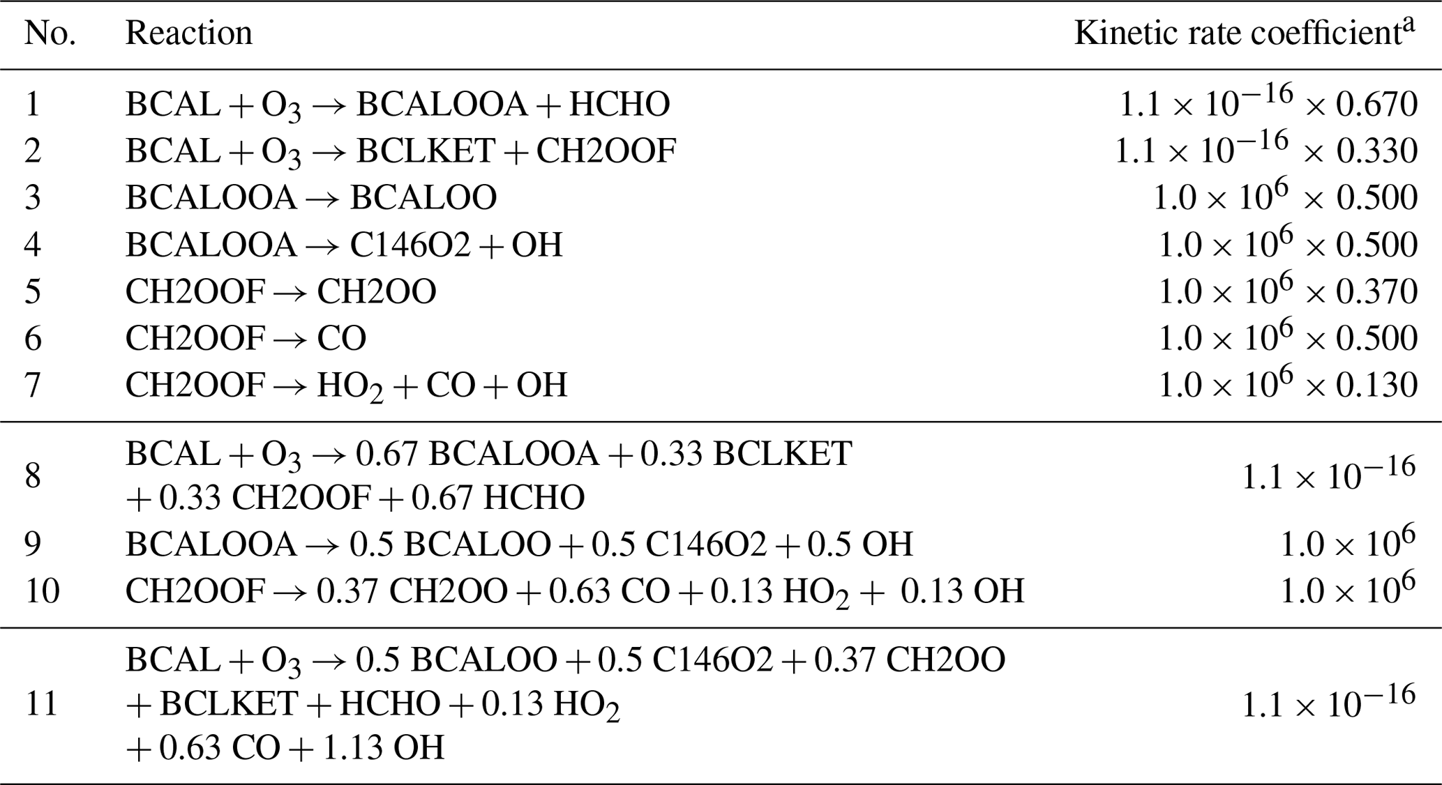
a The kinetic rate coefficients are given in units of per second (s−1) for unimolecular reactions and in units of cubic centimeters per molecule per second (cm3 molec.−1 s−1) for bimolecular reactions.
2.2 Reduction strategies
GENOA supports four types of reduction strategies:
-
removal – reactions, species, or gas–particle partitioning with negligible effects on SOA formation are removed from the mechanism;
-
jumping – one compound is substituted by its oxidation product, as if the compound had been “jumped over” in the reaction pathway;
-
lumping – compounds with similar properties are combined to form a new compound;
-
replacement – one compound is replaced by another existing compound with similar properties.
The reduction strategies are illustrated with examples from the BCARY reduction in Sect. 2.2.1 to 2.2.4. A detailed list of all of the options and parameters controlling the BCARY reduction is summarized in the Supplement.
For the BCARY reduction, the reduction strategies are employed in the following order: removing reactions, jumping, lumping, replacement, removing species, and finally removing gas–particle partitioning. The reduction strategies are ordered based on their potential influences on the mechanism. The first applied strategies, removing reactions and jumping, trim trivial reactions and species without altering the properties of the species. They are followed by lumping and replacement (as an extension to lumping), which refine the mechanisms considerably by merging the species and reactions involved. Afterward, the removing species strategy attempts to delete all merged and unmerged species. Finally, the strategy of removing gas–particle partitioning is applied in order to remove the partitioning of condensable species, which cannot be removed by removing species. This current order has been tested and found to be efficient for the BCARY mechanism, but it can be changed by the user along with other user-defined parameters.
2.2.1 Removal strategy
The removal strategy assumes that chemical reactions and/or species with a low probability of contributing to the formation and evolution of SOA can be eliminated from the mechanism. In general, three types of removal are applied depending on the removed subject:
-
removing reactions;
-
removing compounds in both the gaseous and particle phases (completely removing a species from the scheme);
-
removing the gas–particle partitioning of semi-volatile compounds (consider the semi-volatile compounds as VOCs that do not condense to the particle phase but retain their gas-phase chemistry).
There is no particular restriction to exclude species from the reduction attempt via the strategy of removing species or removing gas–particle partitioning. However, for removing reactions, a threshold on the branching ratio of the reaction is applied to the reduction. The branching ratio is defined as the ratio of the destruction rate of one reaction to the sum of the destruction rates of all reactions of the targeted species. In the BCARY reduction, a maximum branching ratio (Brm) is defined as a restriction criterion. All reactions with an hourly branching ratio (averaged over the training conditions) under this value (reactions that are likely to have a minimal effect on SOA formation) are considered candidates for removal.
To avoid over-reduction, a small Brm is applied at the beginning of reduction. After going through the reductions for all reduction strategies, the value of Brm is then incremented. In the reduction of BCARY, an ascending list of Brm values equal to 5 %, 10 %, and 50 % is employed, which is changed to 10 %, 50 %, and 100 % at the late stage (explained in Sect. 2.5). When Brm equals 100 %, GENOA evaluates the removal of each reaction.
2.2.2 Jumping strategy
The jumping strategy relies on the assumption that compounds can be skipped in successive reactions, as long as they do not adversely impact the SOA concentration. In other words, the predecessor of an organic compound may directly form its destruction products. The jumping strategy is perfectly suited to intermediate compounds whose fast degradation may cause numerical stiffness, commonly including radicals, such as oxy radicals (RO) or alkoxy radicals (ROO), as well as Criegee intermediates.
Table 2Reactions before and after the jumping strategy, where the MCM species BCALOO is jumped over by its degradation product BCLKET.

a [H2O] is the concentration of H2O. b Reaction (R1) is updated from reaction no. 11 in Table 1.
As shown in Table 2, the Criegee intermediate BCALOO, formed during the ozonolysis of BCAL (reaction no. 11 in Table 1), is jumped over to its only destruction product BCLKET. Consequently, reaction nos. 12 to 16 are removed, and reaction no. 11 is updated to Reaction (R1) (“R” for reaction after reduction strategy).
There are similarities between reduction by jumping and prereduction in the sense that both can jump reactions without affecting organic compounds. However, the two processes serve different purposes, as prereduction is intended to provide a reliable reference mechanism for training, whereas jumping is used in training to search for possible reductions. On the one hand, the current prereduction only reduces very fast degraded radicals that undergo a single unimolecular reaction with a constant kinetic rate coefficient (e.g., no temperature effect). In this case, one species may lead to several degradation products. As these reactions are extremely fast and independent of atmospheric conditions, they only cause numerical issues in simulation and should be removed from the reference mechanism. On the other hand, jumping may be relatively slow or affected by environmental conditions; therefore, an evaluation is necessary. Jumping is currently limited from one species to another at a time. The difference in carbon numbers between reduced species can not exceed three in order to prevent significant differences in organic mass before and after jumping. As shown in Table 2, the degradation of BCALOO into BCLKET involves five bimolecular reactions, which may affect SOA formation under different atmospheric conditions (e.g., with different inorganic concentrations and relative humidity, RH).
Table 3Explicit reactions of the MCM species BCAO2, BCBO2, and BCCO2 in the degradation scheme of β-caryophyllene (BCARY).
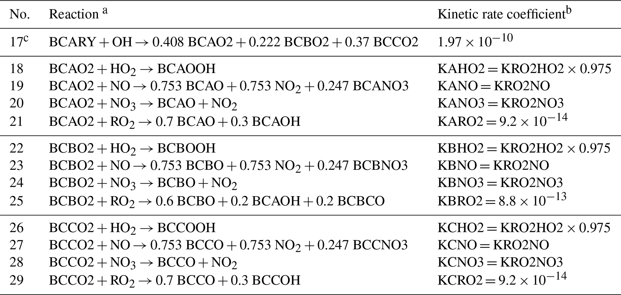
a Species RO2 represents the sum of all peroxy radicals. b The same symbols are used to demonstrate the reduction strategies shown in Tables 4 and 5. The precise values of kinetic rate coefficients (i.e., KRO2HO2, KRO2NO, and KRO2NO3) can be found on the MCM website (v3.3.1, http://mcm.york.ac.uk/home.htt, last access: 25 April 2022) (in cm3 molec.−1 s−1). c Reaction no. 17 shows the production of BCAO2, BCBO2, and BCCO2, whereas the other reactions (nos. 18 to 29) depict their destruction processes.
2.2.3 Lumping strategy
The lumping strategy (i.e., lumping different compounds into a single surrogate compound) assumes that organic compounds with similar chemical structures may exhibit similar properties and undergo similar physicochemical processes and may, therefore, be lumped together. With lumping, both the number of species and reactions decrease.
Table 4Reduced reactions of Table 3 via the lumping strategy, in the case of lumping BCAO2, BCBO2, and BCCO2 into a new surrogate mBCAO2. The name of the new surrogate contains the letter “m” for “merged” and the name of the relatively dominant lumped species. This notation of lumping is used hereafter.
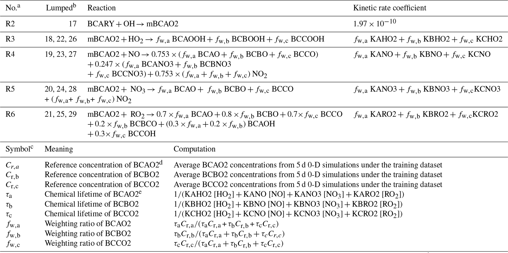
a The reaction number after lumping, where Reactions (R3) to (R6) preserve the destruction of BCAO2, BCBO2, and BCBO2, and Reaction (R2) presents the production. b The reaction numbers before lumping as presented in Table 3. c The subscript letters a, b, and c stand for BCAO2, BCBO2, and BCCO2, respectively. d The calculation method also applies to other BCARY-derived organics. e [X] in the calculations is the reference concentration of radical and other inorganic species, where X is HO2, NO, NO3, or RO2 in this case. For radicals derived from the SOA precursor, the reference concentration is the produced concentration without considering their rapid destruction.
The lumping strategy is illustrated by the comparison of Table 3 (reactions before lumping) and Table 4 (reactions after lumping). In this example, a total of 13 chemical reactions (nos. 17 to 29) involving three organic compounds are reduced to five reactions (a production reaction, Reaction R2, and four destruction reactions , Reactions (R3) to (R6), of the new surrogate).
As demonstrated in the tables, the organic compounds BCAO2, BCBO2, and BCCO2 from the original MCM scheme are the peroxy radicals formed from the OH-initiated oxidation of β-caryophyllene (Table 3). It is evident from their structures (shown in Fig. C1) that they are isomers and may share similar chemical properties. When applying the lumping strategy, BCAO2, BCBO2, and BCCO2 are merged into a new surrogate named “mBCAO2” (Table 4). Additional lumping examples are provided in Appendix C1, describing the lumping of compounds with differing structural groups derived from different oxidation reactions.
The key parameter that drives the reduction accuracy is the “weighting ratio” of lumping (fw), corresponding to the weight of the original species in the new surrogate compound. As detailed in Table 4, fw is computed as a function of the chemical lifetime τ following the computation of Seinfeld and Pandis (2016), and the reference concentrations Cr that are the arithmetic mean concentrations calculated from 0-D simulations using the reference mechanism. Both τ and Cr are based on the averages of simulations across all training conditions. The properties of the new surrogate compound (e.g., molecular structure, saturation vapor pressure, molar mass, and degradation kinetics) are estimated by weighing the properties of the initial compounds, whereas the stoichiometric coefficients and the kinetic rate coefficient of the new reaction are obtained by weighing those of the initial reactions.
Chemical lifetimes and reference concentrations may be close for species that share similar structures and undergo analogous reactions. In cases where these species originate from the same reaction, they can be lumped directly, with the branching ratios of the formation reaction serving as weighting ratios. As an example, BCAO2, BCBO2, and BCCO2 undergo equivalent reactions, with the exception of the RO2 reaction of BCBO2. As the BCARY degradation is not very sensitive to RO2, BCAO2, BCBO2, and BCCO2 can be lumped together with fw,a, fw,b, and fw,c equal to the branching ratios of reaction no. 17, i.e., 0.408, 0.222, and 0.37, respectively.
Most lumping involves species that are not isomers and undergo different reactions, which makes lumping multiple species at the same time highly uncertain. Therefore, in practice, GENOA attempts to lump only two species in a single reduction in order to ensure the effectiveness of computation. A lumping of multiple species can be achieved by combining several reductions (e.g., first lumping BCAO2 with BCCO2 to form mBCAO2 and then lumping BCBO2 into mBCAO2).
In BCARY reduction, lumping is subject to certain restrictions:
-
There should be no lumping between a compound and its oxidation products.
-
Compounds with specific structural groups sharing common chemical behavior may be more appropriately merged together. Thus, compounds containing peroxyacetyl nitrate (PAN), organic nitrate (RONO2), organic radical (R), oxy radical (RO), peroxy radical (RO2), carboxylic acid (RC(O)OH), and peroxycarboxylic acid (RC(O)OOH) functional groups can only be lumped with compounds containing the same groups.
-
The difference in the molecular weight should be negligible (i.e., smaller than 100 g mol−1).
-
The difference in the carbon number should be no more than two.
-
The difference in the chemical lifetime should be less than 10-fold.
-
Lumping is not considered for biradicals (ROO) that degrade rapidly into closed-shell molecules, as jumping is considered to be more appropriate for these compounds.
The difference in saturation vapor pressure between “lumpable” condensables is not explicitly restricted in BCARY reduction. However, it is implicitly considered, as GENOA searches and attempts to lump species with similar saturation vapor pressures first. Nonetheless, the user can activate the option to limit the range of saturated vapor pressure differentials between lumpable condensables, along with other user-defined reduction options listed in the Supplement.
2.2.4 Replacement strategy
The replacement strategy assumes that a compound with a negligible contribution to SOA formation can be substituted by a compound with a similar structure or undergoing the same reactions. In comparison to lumping, the replacement strategy reduces the number of reactions/species without creating new surrogate species.
Table 5Reduced reactions of Table 3 via the replacement strategy, in the case of replacing BCBO2 and BCCO2 with one existing species – BCAO2.
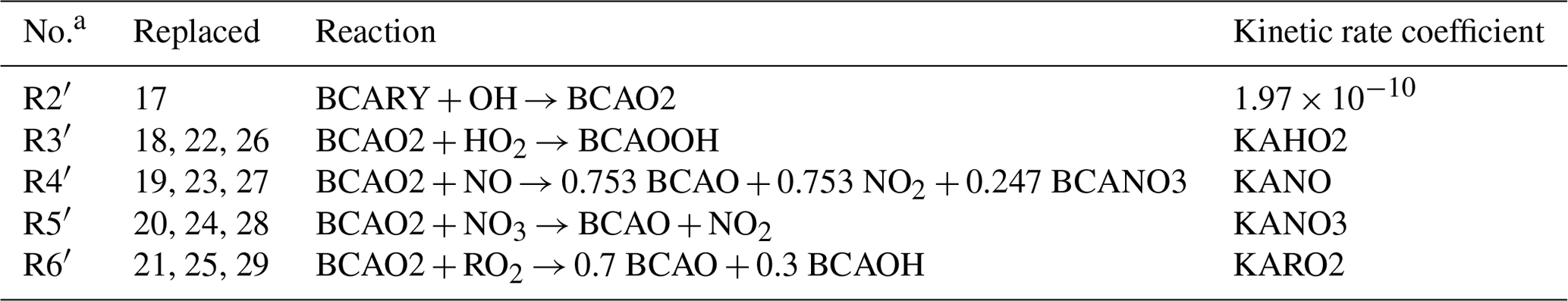
a The symbol ′ is used to distinguish the reactions in this table from the corresponding number of lumping reactions in Table 4.
Table 5 illustrates a reduction occurring via the replacement strategy (to be compared to the original mechanism in Table 3), assuming that BCAO2 is predominant in SOA formation. By substituting both BCBO2 and BCCO2 with BCAO2, the OH reaction of BCARY only leads to the production of BCAO2. The MCM reaction nos. 17 to 29 can then be reduced to Reactions (R2′) to (R6′) via replacement.
The replacement strategy (Table 5) is expected to reduce the computational time more than the lumping strategy (Table 4), as all reactions originating from the replaced species are removed from the mechanism. Hence, it does not require the computation of weighting ratios and new surrogates. However, as a compromise, replacement could be less accurate than lumping, as replacement may discard some compounds and part of the mechanism, thereby leading to more error.
Thus, in an effort to prioritize the accuracy of reduction, GENOA currently employs replacement only after lumping and exclusively on species from the same reaction. In this way, species that were not lumped (because lumping was rejected or because they do not respect the lumping restriction) can be reduced by replacement. During the training of BCARY reduction, a restriction is applied on small organic compounds with a molar mass of less than 100 g mol−1, which are excluded from replacement. The difference in carbon number is no more than three.
Overall, the searches for viable reductions are conducted in reverse order of the reaction/species list. For removal, GENOA attempts to remove reactions from the bottom of the list and moves to the previous reactions. The same reverse sequence is followed for other strategies. When applied to the jumping strategy, for instance, GENOA tries to jump the species that has the highest generation and then move down to the species that has the lowest generation. Among all reduction strategies, only lumping alters the saturation vapor pressure of condensable species. Therefore, a rank of saturation vapor pressure is used exclusively in lumping to determine the most appropriate lumpable species. At each reduction, GENOA attempts to reduce only one species/reaction via removal or one pair of compounds via lumping/replacing/jumping. This restriction allows exhaustive tracking of every detailed modification and its effect on SOA concentrations.
2.3 Datasets of atmospheric conditions applied to reduction
All of the atmospheric conditions applied to the reduction are extracted from a 3-D simulation spanning the latitudes from 32 to 79∘ N and the longitudes from 17∘ W to 39.8∘ E over continental Europe in a 1-year period (2015) using the CHIMERE chemistry transport model. The CHIMERE model and the configuration used for the simulation are described in Lanzafame et al. (2022). The 3-D CHIMERE simulation was conducted with the implicit gas-phase MELCHIOR2 mechanism (Derognat et al., 2003), which contains 120 reactions and less than 80 lumped species. The MELCHIOR2 mechanism describes the degradation of sesquiterpenes by three oxidant-initiated reactions (HUMULE reacts with OH, O3, and NO3, respectively), where the species HUMULE represents the lumped class of all sesquiterpenes.
The monthly diurnal profiles of hourly meteorological data (e.g., temperature and RH) as well as the hourly concentrations of oxidant, radical, and other inorganic species were extracted from each location. This information is required in the 0-D simulations with SSH-aerosol (see Sect. 2.4) to reproduce SOA concentrations and compositions under near-realistic conditions. As the reduced SOA mechanism focuses only on SOA formation, the meteorological data and the concentrations of oxidants, radicals, and inorganics are assumed to remain intact during the 0-D SOA simulation. The coordinates and time of each condition are also provided to calculate the solar zenith angle. The concentration of HUMULE (denoted CSQT as the CHIMERE surrogate for sesquiterpene) is used to estimate the SQT concentration. For the purpose of calculating reduction parameters (e.g., the weighting ratio fw and the branching ratio B) and evaluating the reduced mechanisms, a dataset of representative physiochemical conditions extracted from CHIMERE simulation results is employed in GENOA. Depending on their usage, three groups of conditions are defined: the training dataset, the pre-testing dataset, and the testing dataset.
2.3.1 Training dataset
The training dataset is the set of conditions used to initialize the reduction parameters, estimate the reference concentrations, and evaluate the reduced mechanisms. For a mechanism containing over 1000 reactions and 500 species, a complete reduction may require more than 10 000 SOA simulations to evaluate all of the reduction attempts. To reduce the number of simulations and the computational cost, a limited number of conditions can be evaluated at each reduction attempt.
For the reduction of BCARY degradation, a training dataset of eight conditions is selected, which contains six chemistry-relevant conditions and two additional meteorological conditions. The geographic and meteorological information of each condition is described in Table 6, where the conditions cover a broad range in time (summer and winter conditions), temperatures ranging from 260 to 302 K, and RH values from 39 % to 89 %.
Table 6Geographic and meteorological conditions of the training dataset. The table headings, from left to right, indicate the name, latitude, longitude, time period, average temperature, average RH, average daily NO reaction ratio, and simulated total SOA concentration of the training conditions.
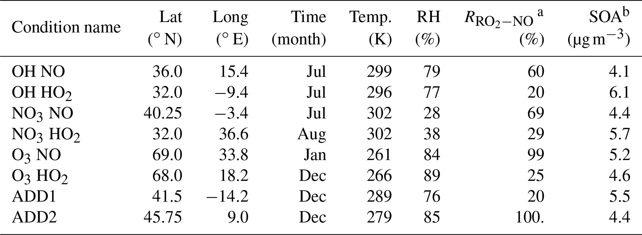
a The average daily NO reaction ratio is calculated using the RO2 reactivity of NO, HO2, NO3, and RO2. Conditions with a high RNO ratio are considered in the high-NOx regime. b SOA is simulated with an initial BCARY concentration of 5 µg m−3.
The six chemistry-relevant conditions, which are named after the dominant oxidants (OH, O3, and NO3), focus on the influences of chemical regimes on SOA formation under either a high-NOx regime (represented by high NO concentrations) or a low-NOx regime (represented by high HO2 concentrations). The two additional conditions included in the training dataset to improve the reduction are referred to as ADD1 and ADD2.
The chemical regimes of the different conditions can be illustrated by seven competitive reaction ratios (equations are listed in Appendix Table C1):
-
The reaction ratios of the precursor with the oxidants O3 (), OH (ROH), and NO3 (), whose sum equals 1, indicate the relative reactivity of the first-generation oxidation pathways that lead to the formation of distinct kinds of RO2 species.
-
The reaction ratios of RO2 species with NO (), HO2 (), NO3 (), and other RO2 species (), whose sum equals 1, indicate the relative reactivity of successive reactions with RO2 species.
These ratios indicate the competition between autoxidation and bimolecular reactions that result in different SOA types. A combination of these seven reaction ratios determines the chemical regime and favorable reaction pathways under a given atmospheric condition.
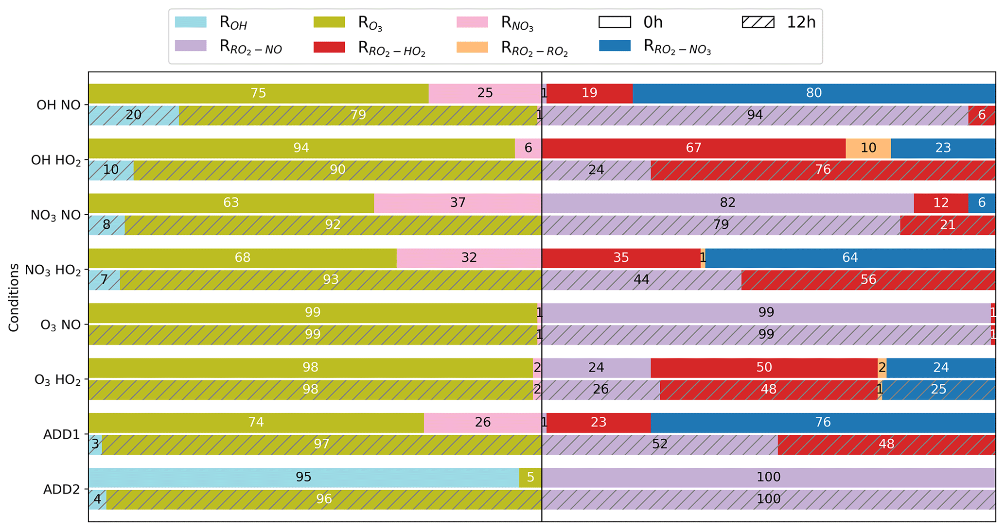
Figure 2A bar plot showing the occupancy of seven reaction ratios in the BCARY initiation reactions and RO2 reactions, under the training conditions at midnight (00:00 GMT+1, top bar) and noon (12:00 GMT+1, bottom bar with hatching). From left to right, six ratios are presented on each bar in the following order: , ROH, , , , , and (no display if ratio is zero). Table C1 provides the equations for calculating the reaction ratios.
Figure 2 describes the reaction ratios at midnight (00:00 h) and noon (12:00 h) for the training conditions. Under the majority of atmospheric conditions, O3 is the dominant oxidant of BCARY due to the carbon–carbon double bonds that are subject to ozonolysis. The high-O3 training conditions have a ratio exceeding 98 % at both noon and midnight. The bimolecular reactions with NO and HO2 dominate RO2 reactions in the MCM mechanism. Due to the low kinetic rate constants and low concentrations, the ratios of OH and NO3 reacting with BCARY are relatively low (under 40 %). The high-OH conditions are determined by the OH ratio at noon, whereas the high-NO3 conditions are determined by at midnight. One specific exception is the additional condition ADD2, which is located in the northern part of Italy, within the Alpine arch, close to the metropolitan city of Milan. This condition is in the extremely high NOx regime, as high concentrations of NO are transported from polluted areas. These high NO concentrations consume O3 and NO3, causing low concentrations of O3 and NO3. At night, ADD2 has a high ROH ratio of 95 % at midnight that is not due to an abundance of OH but rather to extremely low concentrations of O3 (2.9 × 10⁻⁴ ppb) and NO3 (1.1 × 10⁻⁹ ppb) which lead to an absence of nighttime reactivity.
2.3.2 Pre-testing dataset
The pre-testing dataset contains a greater number of conditions than the training dataset, covering the major atmospheric conditions encountered across the domain. After the mechanism has been significantly reduced, the pre-testing dataset is included along with the training dataset in order to evaluate the reduction attempts at the late-stage reduction. At this point of reduction, a slight change in the mechanism significantly impacts the SOA concentrations; therefore, merely evaluating reduction based on the training dataset may not be adequate. Meanwhile, the size of the mechanism has already been significantly reduced, which makes the evaluation of each reduction attempt on the pre-testing dataset less computationally expensive.
In principle, the pre-testing dataset should be able to provide a fairly accurate representation of the testing dataset. However, this may not always be the case, as the pre-testing dataset is selected almost randomly from the testing dataset. Therefore, an adjustment may be required to increase the representativeness of the pre-testing dataset by adding or removing a few conditions. For the application to BCARY, a pre-testing dataset with 150 atmospheric conditions is selected from the testing dataset. The pre-testing dataset consists of 50 conditions for each level (low, medium, and high) of SQT emissions (see Sect. 2.3.3). The locations of the training and pre-testing conditions are presented in Fig. 3.
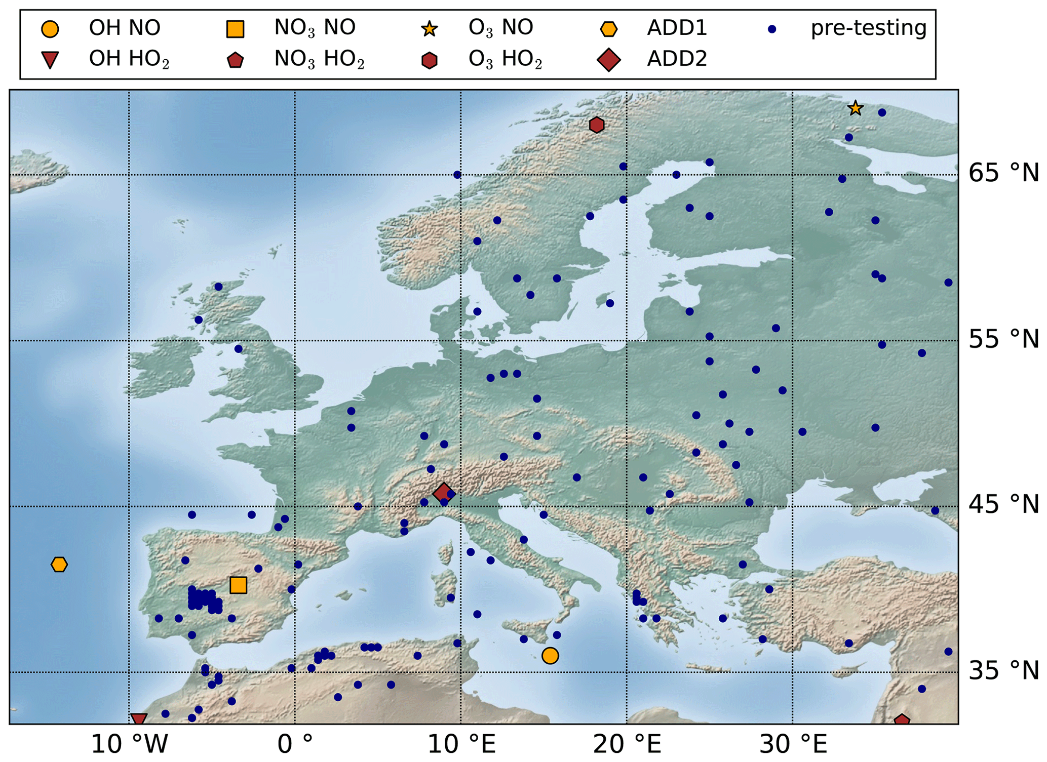
Figure 3Simulation domain and locations of training (see the figure legend) and pre-testing (blue scattered dots) datasets applied to the reduction.
2.3.3 Testing dataset
The final reduced mechanism, obtained from training, is eventually evaluated with a large number of atmospheric conditions in the testing section. This set of conditions for the final evaluation is referred to as the testing dataset. Among all datasets, the results on the testing dataset are most likely to reflect the actual performance of the reduced mechanism for 3-D modeling.
In the BCARY reduction, the testing dataset is selected based on the concentrations of the CHIMERE sesquiterpene surrogate. Its maximum hourly concentration CSQT in parts per billion (ppb) is used to exclude conditions with a negligible SQT concentration. A testing dataset within a total of 12 159 conditions is applied (see Sect. 3.2), including all conditions (2159 conditions) with a high SQT concentration (CSQT≥0.1 ppb), 5000 random select conditions with a medium SQT concentration (CSQTϵ between 0.01 and 0.1 ppb), and 5000 random select conditions with a low SQT concentration (CSQTϵ (0.001, 0.01]). The conditions with an extremely low SQT concentration (CSQT<0.001 ppb) are not included in the testing dataset. Figure B1 indicates the locations of the testing dataset as well as the testing results for BCARY reduction.
2.4 Settings for SOA simulations
The chemical composition and temporal variation in SOA due to gas-phase chemistry and condensation/evaporation are simulated using the 0-D aerosol module SSH-aerosol (Sartelet et al., 2020). As detailed in Couvidat and Sartelet (2015), the gas–particle partitioning is estimated with Raoult's law (for the partitioning between the gas phase and the organic phase) and Henry's law (for the partitioning between the gas phase and the aqueous phase). Therefore, some properties of condensable compounds, such as the saturation vapor pressure Psat and the decomposition into functional groups, are crucial for modeling. For BCARY-derived organics, Psat is calculated using UManSysProp (Topping et al., 2016). The vapor pressure is computed using the method of Nannoolal et al. (2008) and the boiling point estimation from Joback and Reid (1987). These methods were selected because they provide the best performance when compared with the chamber experiment data of Chen et al. (2012) and Tasoglou and Pandis (2015), as discussed in Appendix A. Furthermore, the activity coefficient γ is calculated with the UNIQUAC Functional-group Activity Coefficients (UNIFAC) thermodynamic model (Fredenslund et al., 1975) for short-range interactions and the Aerosol Inorganic–Organic Mixtures Functional groups Activity Coefficients (AIOMFAC) model for medium-range and long-range interactions (Zuend et al., 2008).
Unless stated otherwise, two simulations are performed for each condition starting at midnight (00:00 h) and noon (12:00 h), considering both the daytime and nighttime chemistry. All 0-D simulations are run for 5 d in order to adequately consider SOA formation and aging processes. The initial BCARY concentration is set to 5 µg m−3 in order to ensure high SOA production (the SOA concentration is always greater than 1 µg m−3 under all evaluated conditions). For optimal computational efficiency, the gas–particle partitioning is assumed to be at thermodynamic equilibrium.
2.5 Settings for evaluation
For the different datasets, the performance of the reduced mechanism on SOA concentrations is evaluated using the fractional mean error (FME) computed with Eq. (1), where Cval,i and Cref,i denote the SOA mass concentration at time step i simulated with the reduced and the reference mechanisms, respectively.
The error of one simulation is defined as the larger of the FME on day 1 and the FME on days 2 to 5, in order to address the difference in the performance of the reduced mechanisms in the early stage of the simulations (SOA formation dominates) and in the later stage (SOA aging dominates). This error is used to evaluate reduction by comparing it to the error tolerance specified in training. For the evaluation on the training dataset, two errors are estimated compared to the previously verified reduced mechanism with a tolerance denoted ϵpre and to the reference mechanism with a tolerance denoted ϵref. The error tolerances are used to restrict both the maximum and the average (half of the tolerance) errors of the training conditions. As for the evaluation on the pre-testing dataset, the error compared to the reference mechanism is calculated. The error tolerances and are set to the average and maximum errors, respectively.
In order to begin with a conservative BCARY reduction, the initial values of ϵpre and ϵref are both set to 1 %. The values of these error tolerances are then increased to larger values, reflecting the looser criteria used throughout the reduction. ϵref is used to track the performance of the reduction, while ϵpre is used to avoid large errors introduced by one reduction attempt. Therefore, ϵpre is lower than or equal to ϵref. For every 1 % increase in ϵref, ϵpre is stepped up by 1 % from 1 % to the value of ϵref. By doing this, GENOA first accepts reductions that introduce small errors compared with the previously validated mechanism and then accepts reductions that introduce larger errors up to ϵref.
The maximum values for both ϵref and ϵpre are set to 10 %. When ϵref reaches 3 %, the mechanism is expected to be largely reduced. From then, the evaluation under the pre-testing dataset is considered to be added to the reduction. This means that all subsequent reductions are evaluated using both the training and pre-testing datasets. The average and maximum errors ( and ) are restricted to be lower than 3 % and 20 %, respectively. As a result of the above error tolerances, a reduced SQT SOA mechanism with an average inaccuracy on SOA formation lower than 3 % (maximum 20 %) is expected.
Additionally, another error factor noted as the fractional bias (FB, computed as detailed in Eq. 2) is used to visualize the temporal performance of the reduced mechanism at each simulation time step. As examples, Figs. 8 and 10 show the average FB at each time step for the pre-testing conditions.
When trying to remove reactions, GENOA first removes reactions with low hourly branching ratios (Brm≤5 %), as the removal of reactions with Brm is likely to have a minimal effect on SOA formation. After no reduction is accepted by all applied reduction strategies under the defined error tolerance, the value of Brm is increased to 10 % and then 50 %.
2.6 Settings for aerosol-oriented treatments
In late-stage training, an intense competition between different potential reductions is observed, and a minor modification may induce significant uncertainty in the mechanism and prevent further reduction. Moreover, because the formation of aerosols costs more CPU time than gas-phase chemistry, specific treatments are employed in the late stage of training to reduce the number of condensable species preferentially. These treatments, which reduce species rather than reactions, are done when the size of the mechanism is below a certain threshold. For BCARY reduction, the treatments are activated once the number of condensable species has decreased to 20. Consequently, late-stage treatments encourage reduction via the removal of condensable species and are referred to as aerosol-oriented treatments. The treatments consist of the following:
-
Restriction of the reduction of the number of reactions is applied; thus, strategies that reduce the number of aerosols are favored to result in fewer condensable species.
-
The evaluation of aerosol-oriented reductions on the training dataset is bypassed when applied to jumping, lumping, and replacement. As a result, the aerosol-oriented reduction is evaluated only on the pre-testing dataset to avoid being rejected under some of the extreme conditions in the training dataset (which are less representative of average atmospheric conditions than the conditions of the pre-testing dataset).
-
An additional type of removal is applied – removing elementary-like reactions.
The additional reduction strategy of removing elementary-like reactions is targeted at reactions with multiple products. After rewriting the reaction into a set of elementary-like reactions, each with one oxidation product and integer stoichiometric coefficient, GENOA investigates the possibility of removing the elementary-like reactions one by one. In practice, removing elementary-like reactions is inserted after the strategy of removing reactions and before jumping, when no further reduction that reduces condensable species can be found with the current parameters.
GENOA is applied to the SQT degradation mechanism of v3.3.1 of the Master Chemical Mechanism (Jenkin et al., 2012). Here, β-caryophyllene (BCARY) is considered a surrogate for SQT primary VOCs. The degradation of β-caryophyllene in the original MCM mechanism consists of 1626 reactions and 579 species (223 radicals and 356 stable species). After prereduction, the mechanism contains 1241 reactions and 493 species (137 radicals and 356 stable species); this is employed as the starting point and the reference for the reduction (hereafter referred to as MCM).
Moreover, at the beginning of the GENOA training, all of the stable species are assumed to be condensable (referred to as condensables), and their saturation vapor pressures and activity coefficients are calculated based on their molecular structures (as detailed in Sect. 2). Applying the effective partitioning coefficients (Kp at 298 K) described by Seinfeld and Pandis (2016), condensables can be classified into semi-volatile organic compounds (SVOCs; Kp between 10−2 and 10 m3 µg−1), low-volatility organic compounds (LVOCs; Kp between 10 and 104 m3 µg−1), and extremely low volatility organic compounds (ELVOCs; Kp larger than 104 m3 µg−1).
The semi-explicit SQT SOA mechanism “Rdc.” presented in this section is trained from MCM with GENOA. Detailed descriptions of the building process and its chemical scheme are provided in Sect. 3.1. By the end of the training, Rdc. is reduced from MCM to only 23 reactions and 15 species (see Appendix B for the reaction and species lists). The size of the Rdc. mechanism is of the same order of magnitude as the BCARY degradation scheme of Khan et al. (2017) (28 reactions and 15 species) used for global modeling. As presented in Sect. 3.2, the Rdc. mechanism accurately reproduces the SOA concentration and composition simulated by MCM with only six condensables. Table B3 summarizes the new surrogates and the lumped MCM species that are included in the final Rdc. mechanism.

Figure 4Reduction process of the Rdc. mechanism showing the decrease in the number of reactions, species, and condensables; the evolution of the average error on the pre-testing dataset (ϵpre−testing, with an error tolerance of 3 %); and the error tolerance compared with MCM (ϵref).
3.1 Building of the reduced SOA mechanism
As shown in Fig. 4, the Rdc. mechanism is built from 113 validated reduction steps. In GENOA, a reduction step refers to all reduction attempts based on the performed reduction strategy and reduction parameters, while a validated reduction step indicates at least one reduction attempt has been accepted at this step. The entire building process can be divided into three stages:
-
Early stage refers to the period from the 1st to the 74th reduction step. By the end of the 74th reduction step, the mechanism is reduced to 68 reactions and 41 species (including 20 condensables). The early-stage reduction is trained only on the training dataset with the seven pre-described reduction strategies. After ϵref reaches 3 %, the list of Brm is changed from [5 %, 10 %, 50 %] to [10 %, 50 %, 100 %].
-
Late stage I spans from the 75th to the 107th reduction step. By the end of the 107th reduction step, the reduced mechanism consists of 38 reactions and 19 species (including seven condensables), and no further reduction can be found within ϵref≤10 % and ϵpre≤10 %. In this stage, the reduction is trained on the pre-testing dataset if condensables are removed with jumping, lumping, or replacement. For reduction with other types of reduction strategies, it is first trained on the training dataset and then on the pre-testing datasets. From all of the reduced mechanisms with seven condensables, GENOA selects the one with the minimum average errors on the pre-testing dataset (2.44 %) to start the next stage.
-
Late stage II refers to the period from the 108th to the 113th reduction step. At this stage, the reduction strategy of removing elementary-like reactions is applied to the training. All reductions that reduce the condensables are evaluated exclusively on the pre-testing dataset. The size of the reduced mechanism was reduced to 23 reactions and 15 species, among which the number of condensables is reduced to 6. The average (maximum) error of the final reduced mechanism Rdc. is 2.65 % (17.00 %) under the pre-testing dataset compared with MCM.
Table 7Reduction accomplished per each reduction strategy during the building process of the Rdc. mechanism.
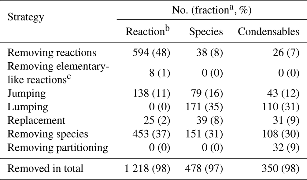
a The fraction of the original number (of reactions or species) that is reduced by the strategy. b The columns, from left to right, are the number (and fraction) of reduced chemical reactions, reduced total gas-phase species, and reduced gas-phase species that can condense on the particle phase, compared with MCM with 1241 reactions and 493 species (356 condensables). c This step is only applied in the reduction at late stage II.
The extent of the reduction due to each strategy is summarized in Table 7. Compared with MCM, up to 98 % of reactions and 97 % of species are reduced in Rdc. As expected, the reduction strategy of removing reactions contributes the most to the decrease in the number of reactions (48 %), followed by the strategy of removing species (with a contribution of 37 %). Meanwhile, both lumping and removing species are significant in the reduction of species (by 35 % and 31 %, respectively). The number of condensables decreases in proportion to the number of species, except for the strategy of removing partitioning. In that case, the gas–particle partitioning is removed and the species remains in the gas phase with no changes in the chemical mechanism.
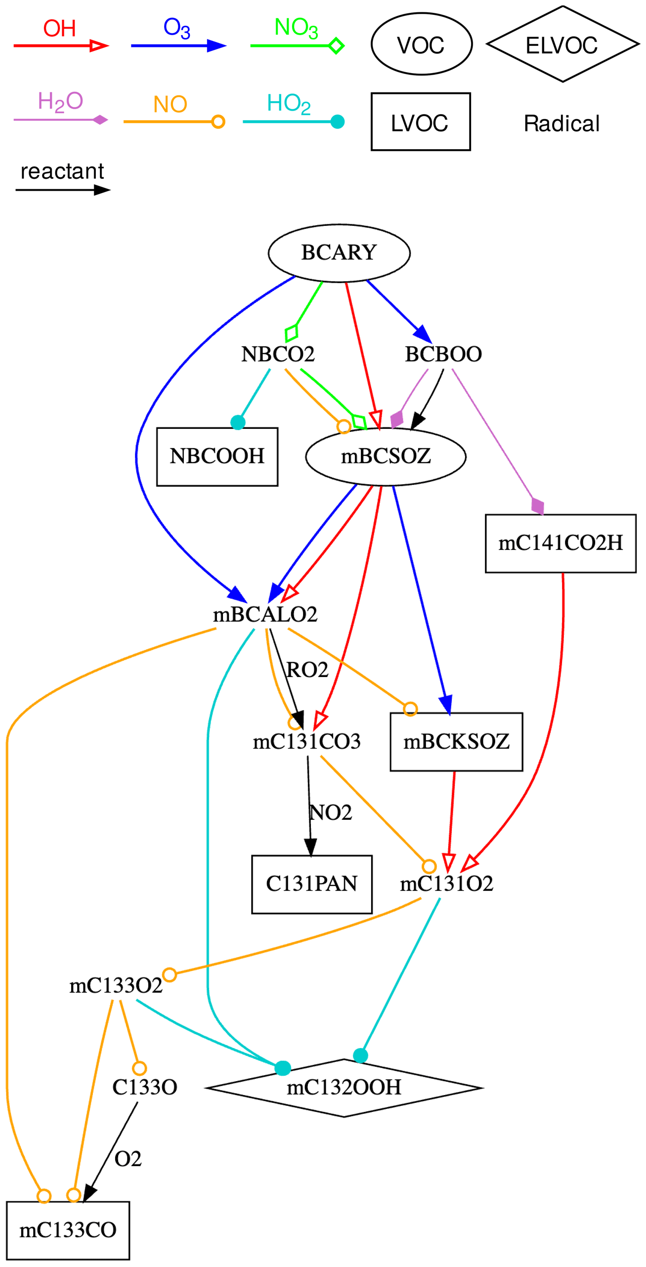
Figure 5Representation of the chemical scheme of the Rdc. mechanism. VOCs, LVOCs, and ELVOCs are presented in ellipse, square, and diamond boxes, respectively. Radicals are written in plain text, without boxes. Reactions with OH, O3, NO3, NO, HO2, and H2O are shown using arrows with different colors and heads (see the figure legend). Other reactants (if any) are labeled near the edges. The complete species and reaction lists of the Rdc. mechanism are given in Appendix Tables B1 and B2, respectively.
As shown in Fig. 5, which describes the chemical scheme of the Rdc. mechanism, the three oxidants (i.e., O3, OH, and NO3) initiated reactions, leading to common oxidation products (e.g., mBCSOZ and mBCALO2) that dominate the successive oxidations. The different reaction pathways under high- or low-NOx regimes are presented in Rdc. with reactions with NO or HO2, respectively, which results in the formation of different types of SOAs: mBCKSOZ, mC133O, and C131PAN (in the presence of NO2) under high-NOx conditions and mC132OOH under low-NOx conditions. Other pathways, such as the bimolecular reactions of the Criegee intermediate BCBOO with water vapor and the RO2 reaction of mBCALO2, are also preserved in the Rdc. mechanism. The six condensables in Rdc. can be categorized into one SVOC, four LVOCs, and one ELVOC, according to the effective partitioning coefficient calculated on the pre-testing dataset. The SOA concentration per volatility class is discussed in Sect. 3.2.
Compared with MCM, Rdc. simplifies a considerable number of reactions that have small impacts on SOA formation (e.g., photolysis reactions) under the majority of atmospheric conditions, and it merges a large number of compounds with similar chemical properties. The main oxidation products from the first two generations of MCM oxidation pathways are preserved mainly through the Rdc. species mBCSOZ, which is a lumped surrogate of several MCM-representative BCARY-derived oxidation products: BSCOZ (the major secondary ozonize with a molar yield of ≥65 %, reported by Jenkin et al., 2012), BCAL (the primary product formed from both OH- and O3-initiated chemistry), and BCKET (from OH-initiated reactions).
3.2 Evaluation of the reduced SOA mechanism
3.2.1 Reproduction of the SOA concentrations
During the testing procedure, the Rdc. mechanism is evaluated at 12 159 locations, with two different starting times (00:00 and 12:00 h). The testing for Rdc. took approximately 2 % of the CPU time consumed for MCM.
Compared with MCM, Rdc. presents a high level of accuracy with an average error of 2.66 % and a maximum error of 17.29 %. The monthly distribution of the number of the testing conditions as well as the testing errors are described in Fig. 6. The error is lower than 10 % for more than 99 % of the simulations. The summer conditions, between June and September, covering more than half of the testing conditions (63 %, 7647 conditions), result in an average error of 2.37 % and a 3rd quartile error of 2.85 %. Compared with the summer conditions, testing results under winter conditions, from October to January (19 % of the testing dataset, 2285 conditions), display slightly higher uncertainty, with an average error of 3.79 % and a 3rd quartile error of 5.36 %.
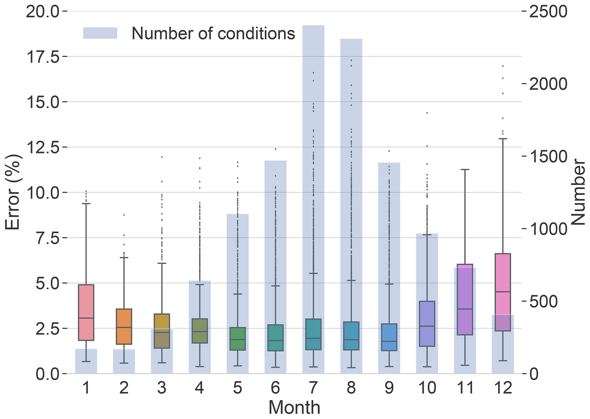
Figure 6Monthly distribution of the testing results (errors compared with MCM) of the Rdc. mechanism in the box plot as well as the number of testing conditions in the histogram.
An error map of testing conditions in July and August is displayed in Fig. 7. It indicates the locations of testing conditions and the errors of each condition, especially highlighting outliers during this period. Detailed error maps of all testing conditions can be found in Appendix B. It shows that the Rdc. mechanism induces low errors (lower than 6 %) for most of the testing conditions. The conditions with errors over 6 % are mainly concentrated in northern Africa near the Atlas Mountains and in the eastern Mediterranean, where the conditions most likely correspond to a dry Mediterranean climate with low RH and high temperature. Other conditions with errors above 6 % are dispersed in the Po Valley of northern Italy and along the coasts of southern Spain. More accurate results could be obtained with stricter parameters for reduction (e.g., lower error tolerance) or by updating the conditions (e.g., training and pre-testing datasets) covering more extreme conditions in the training process.
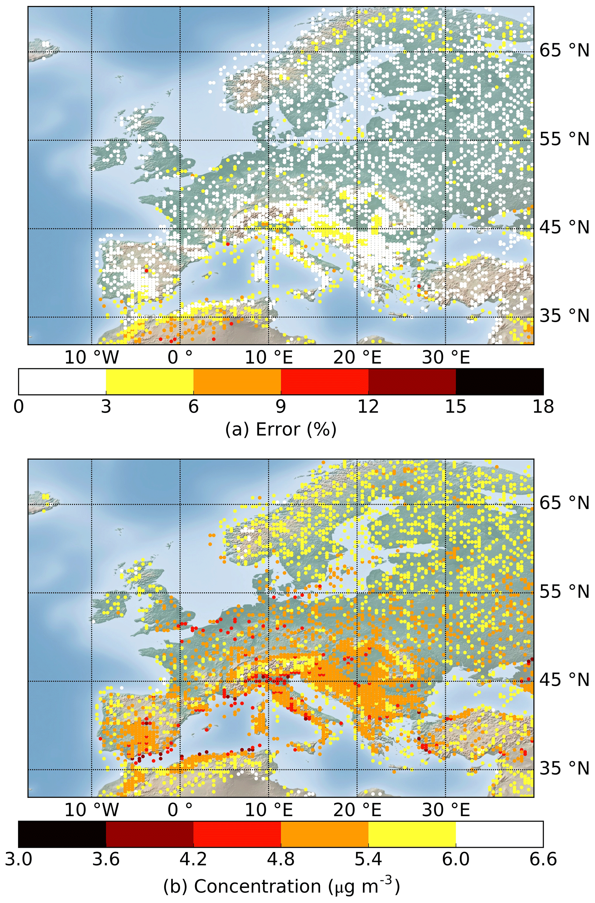
Figure 7Geographic distributions of the (a) error and (b) average SOA concentration of the testing results in July and August simulated using the Rdc. mechanism. The total number of conditions displayed is 4717 out of the 12 159 that were tested. The results of all testing conditions are shown in Appendix B for reference.
3.2.2 Reproduction of the SOA composition
The SOA concentrations and chemical composition simulated with the Rdc. mechanism and with MCM are compared in this section. The temporal profiles of the total SOA concentrations on an average of the pre-testing dataset and nonideal conditions are displayed in Fig. 8. Throughout the entire 5 d simulation period, there is excellent agreement between hourly SOA concentrations simulated with MCM and those obtained from the Rdc. mechanism. The SOA concentration builds up rapidly in the first few hours, where the results of the Rdc. mechanism present relatively larger fluctuations (the maximum FB of 3.74 % is observed at 1 h on the average pre-testing results).
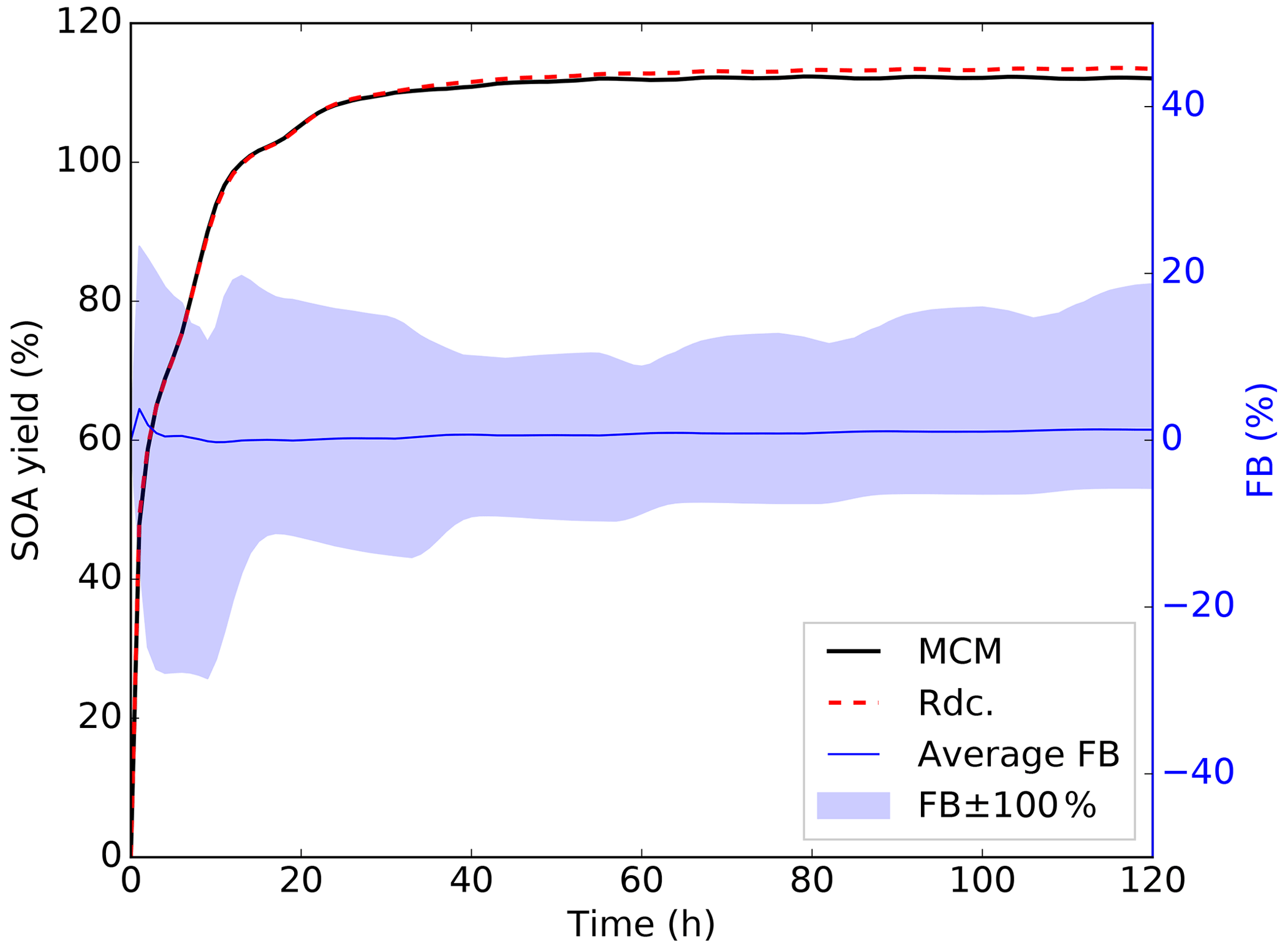
Figure 8Temporal variation in the total SOA concentration simulated with the pre-testing dataset using the MCM (red dashed line) and Rdc. (solid black line) mechanisms under nonideal conditions. The average (solid blue line) and maximum (blue shading) FB values between the MCM and the Rdc. mechanisms are also presented.
The average SOA concentrations per volatility class on the pre-testing dataset at two simulation times (8 and 72 h) are listed in Table 8. At both 8 and 72 h, the Rdc. mechanism accurately reproduces the total SOA mass with a relative difference lower than 0.1 % compared to MCM. An accumulation of the SOA mass into the ELVOC class is observed (51 % of the total SOA mass at 8 h and 66 % at 72 h) with both the MCM and the Rdc. mechanisms. The aging of SOA produces compounds of low and extremely low volatility. Regarding the volatility classes, the Rdc. mechanism tends to slightly overestimate the SOA resulting from ELVOCs and underestimate the SOA resulting from LVOCs, especially at 72 h. This suggests that aging leads to Rdc. condensables of slightly lower volatility than the MCM ones; however, the differences are low (up to 0.4 µg m−3 difference (10 %) at 72 h).
Table 8Average SOA concentrations per volatility class simulated with the MCM and the Rdc. mechanisms on the pre-testing dataset at 8 and 72 h (in µg m−3).
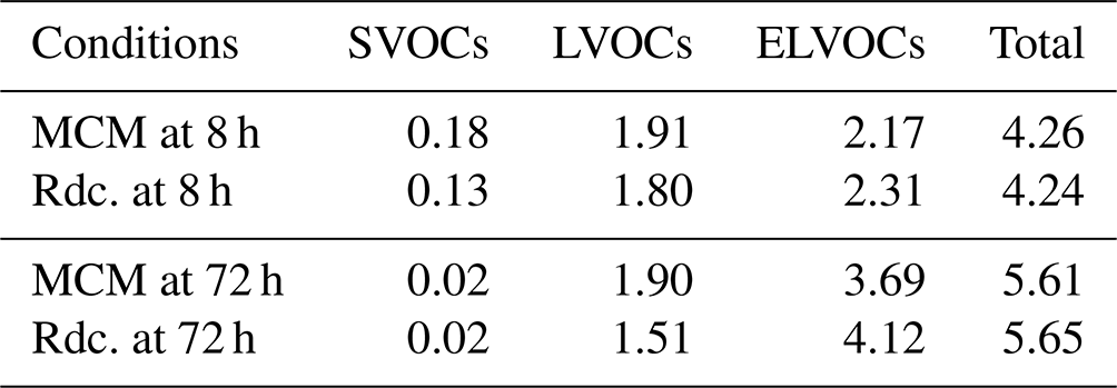
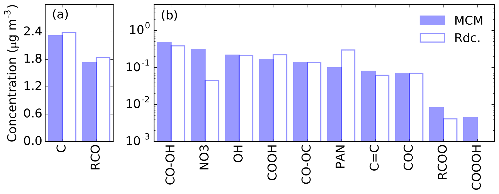
Figure 9Average SOA mass per functional group simulated with the pre-testing dataset using the MCM (blue bar) and Rdc. mechanisms (white bar) at 72 h. The figure is divided into two panels, (a) and (b), due to the large gap in mass between the groups. The labels of the functional groups, from left to right, are as follows: C – carbon bond, RCO – carbonyls (ketone and aldehyde), CO–OH – hydroxy peroxide, NO3 – organic nitrates, OH – alcohol, COOH – carbonyl acid, CO–OC – peroxide, PAN – peroxyacyl nitrates, C=C – carbon double bond, COC – ether, RCOO – ester, and COOOH – peroxyacetyl acid.
The average SOA composition per functional group simulated on the pre-testing dataset at 72 h is displayed in Fig. 9. No significant change in the functional group distributions is found between 8 and 72 h of oxidation. The alkyl (C) and carbonyl groups (RCO) contribute the most to the SOA mass, by more than 1 µg m−3, whereas the other functional groups contribute by less than 1 µg m−3. Overall, the Rdc. mechanism satisfactorily reproduces the composition of the MCM-simulated SOA composition for most functional groups, except for nitrogen-containing groups. In comparison to MCM, only two condensables containing nitrogen are retained in the Rdc. mechanism – NBCOOH and C131PAN – leading to an underestimation of the organic nitrate group (0.31 µg m−3 in MCM and 0.04 µg m−3 in Rdc.) and an overestimation of the nitrate mass of the peroxyacetyl nitrate group (0.10 µg m−3 in MCM and 0.30 µg m−3 in Rdc.). To obtain better results on the reproduction of nitrogen groups, GENOA may be further restricted to distinguish nitrogen compounds in training. Additionally, the peroxyacetyl acid group results in an extremely low SOA mass in MCM (less than 0.01 %); therefore, it is not retained in the Rdc. mechanism.
Moreover, the temporal profiles of the organic mass to organic carbon mass () ratio as well as the , , and atomic ratios are presented in Fig. 10. Comparable patterns are observed in the (1.65 in MCM and 1.63 in Rdc. on average), the (0.37 in MCM and 0.36 in Rdc.), and the (1.62 in MCM and 1.60 in Rdc.) ratios. During the first 8 h of simulation, Rdc. tends to slightly overestimate the and ratios, while the ratio remains fairly stable throughout the entire simulation with a negligible difference (0.02) between MCM and Rdc. The ratio, however, is underestimated by the Rdc. mechanism by 37 % on average (ratio equal to 0.019 in MCM and to 0.012 in Rdc.), indicating the over-reduction of organic nitrites in Rdc. A total of three nitrogen-containing organics (NBCO2, NBCOOH, and C131PAN) are preserved in Rdc., two of which (NBCO2 and NBCOOH) are first-generation products. Therefore, during the first 10 h, the ratio curve simulated by Rdc. drops, whereas it increases in MCM as higher-generation nitrates are produced.
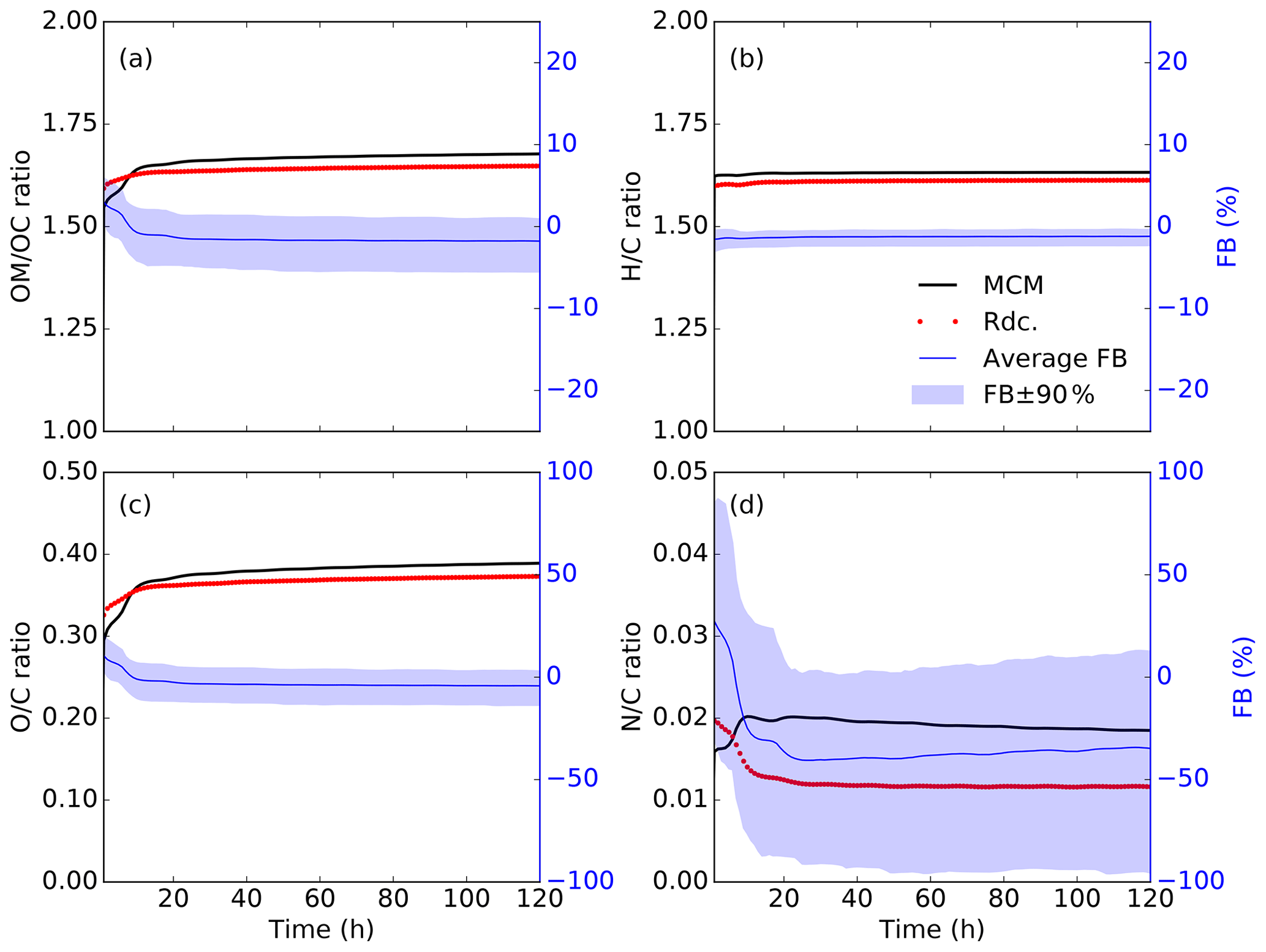
Figure 10Temporal variations in the (a) average organic mass to organic carbon mass () ratio, (b) hydrogen to carbon () atomic ratio, (c) oxygen to carbon () atomic ratio, and (d) nitrogen to carbon () atomic ratio, simulated with MCM (solid black curves) and the Rdc. mechanism (dotted red curves) on the pre-testing dataset. The average FB (solid blue line) and the 90 % range of the FB (blue shading) are also presented.
3.2.3 Sensitivity on environmental parameters
The sensitivities of the Rdc. mechanism to temperature, RH, and SOA mass conditions are investigated with the pre-testing dataset. The default value of the BCARY concentration is 5 µg m−3, and the default RH and temperature are set to constant values of 50 % and 298 K, respectively. As presented in Fig. 11, the SOA yields simulated by the Rdc. mechanism with different environmental parameters show a remarkable resemblance to the SOA yields simulated by MCM.
Under 10 µg m−3, the simulated SOA yields are not affected by the SOA mass loading. This result is consistent with the large contribution of ELVOCs reported in Table 8. A discrepancy of 25 % in the average SOA yield at 1 h with an SOA mass loading of 103 µg m−3 at 1 h and a discrepancy of 8 % at 72 h with an SOA mass loading of 10−3 µg m−3 are observed. The result indicates that the Rdc. mechanism may introduce relatively large uncertainty with extreme SOA loading (larger than 500 µg m−3), which was outside the range of conditions used for the construction of the Rdc. mechanism. SOA formation is affected by RH, due to both the gas-phase chemistry (reaction with H2O vapors) and the gas–particle transfer (condensation of hydrophilic SOA precursors on aqueous aerosols). The sensitivity tests show that the Rdc. mechanism reproduces (differences lower than 2 %) the SOA yields of MCM well with RH values ranging from 5 % to 95 %. For temperature, the Rdc. mechanism reproduces the SOA aging at 72 h very well, but larger discrepancies are observed in the earlier period, when the oxidation products are more volatile. However, the discrepancies in the SOA yield stay low: differences up to 7 % (at 1 and 72 h) and 10 % (at 8 h) are observed for temperatures of 263 and 323 K, respectively. This finding is consistent with the testing results. In summary, the discrepancies suggest that the reduced mechanism performs quite well, although larger discrepancies with MCM are observed under conditions that are outside the range of conditions used during training.
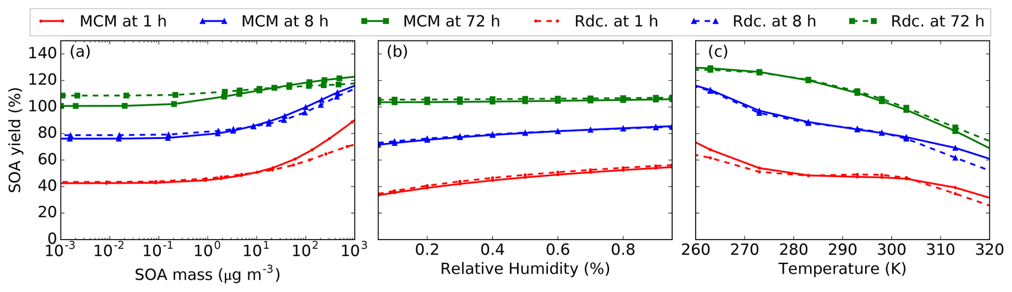
Figure 11Dependence of the average SOA yield simulated by the pre-testing dataset with MCM (solid line) and the Rdc. mechanism (dashed line) on (a) BCARY SOA mass; (b) relative humidity (RH); and (c) temperature at 1 h (red points), 8 h (blue triangles), and 72 h (green squares).
The development and application of the GENerator of reduced Organic Aerosol mechanism (GENOA v1.0) have been presented in this study. GENOA generates semi-explicit SOA mechanisms designed for large-scale air quality modeling by reducing explicit VOC mechanisms with a series of automatic training and testing processes. During the training procedure of GENOA, four types of reduction strategies (removal, jumping, lumping, and replacement) are adopted to locate the potential reduction in the mechanism. Each reduction attempt is evaluated against the explicit mechanism under a sequence of near-realistic atmospheric conditions (the training dataset, and/or the pre-testing dataset at the late stage of reduction). Finally, the reduced mechanism is evaluated under various conditions of a testing dataset. Under each condition, two 5 d 0-D simulations starting at midnight and noon are conducted with the SSH-aerosol model to simulate SOA concentrations and compositions for reduction evaluation.
GENOA successfully generated semi-explicit SOA chemical mechanisms for the degradation of sesquiterpene, for which the explicit β-caryophyllene mechanism of the Master Chemical Mechanism serves as the reference mechanism and the starting point. The final reduced SQT SOA mechanism contains 23 reactions (down from 1626 reactions in MCM), 15 gas-phase species (down from 579 gases), and 6 aerosol species (down from 356 aerosols). It reproduces the SOA formation and aging by introducing an average error of 2.7 % under conditions over Europe with only 2 % of the size of MCM. The SOA volatility is well reproduced with the reduced mechanism, as well as the decomposition into functional groups, and the (1.55 in the Rdc. mechanism and 1.60 in MCM), , and ratios. Nitrogen-containing SOA, which contributes to only 7 % of the total mass, is not as well represented as other groups, and the ratio is slightly underestimated in the Rdc. mechanism (0.016 compared with 0.021 in MCM). The similarity of the representation of the functional group decomposition allows for the similar reproduction of the non-ideality of SOA in the Rdc. mechanism and in MCM. Additionally, the sensitivity tests on RH, temperature, and organic mass loading show that the SOA simulated with the Rdc. mechanism is in good agreement with MCM results under most conditions (except for conditions with extremely high temperature or with massive organic aerosol loading where discrepancies in the SOA yields may reach 8 % (temperature) and 25 % (massive mass loading)). This indicates that the reduced mechanism performs well for conditions in the training range, but its performance may deteriorate for conditions outside of this range. To improve the performance of the semi-explicit SOA mechanism under conditions outside of the training range, two methods can be employed: the first is to include the outlier conditions in the training procedure if they are considered influential to SOA formation, and the second is to adopt strict error tolerance to restrict the reduction.
The ozonolysis experimental data reported in Tasoglou and Pandis (2015) and Chen et al. (2012) are used to evaluate the performance of different computation methods for the saturation vapor pressure of BCARY oxidation products. In our simulations, the saturation vapor pressure is computed by UManSysProp with the SMILES (Simplified Molecular Input Line Entry System) structures of organic compounds. Eight methods are provided in UManSysProp, including SIMPOL.1 (“sim”) of Pankow and Asher (2008), EVAPORATION (“evp”) of Compernolle et al. (2011), and six methods out of the combination of two methods to compute the vapor pressure (“v0”, Myrdal and Yalkowsky, 1997; and “v1”, Nannoolal et al., 2008) and three methods to compute the boiling point (“b0”, Nannoolal et al., 2004; “b1”, Stein and Brown, 1994; and “b2”, Joback and Reid, 1987). As shown in Fig. A1, the SOA distribution simulated with “v1b2” (thin yellow diamonds) agrees best with the experimental data. Therefore, this method with the vapor pressure computed by Nannoolal et al. (2008) and the boiling point computed by Joback and Reid (1987) is used in the BCARY reduction. The results simulated with the final reduced mechanism Rdc. (purple diamonds) is also presented in Fig. A1, which has a great resemblance to the experimental data.
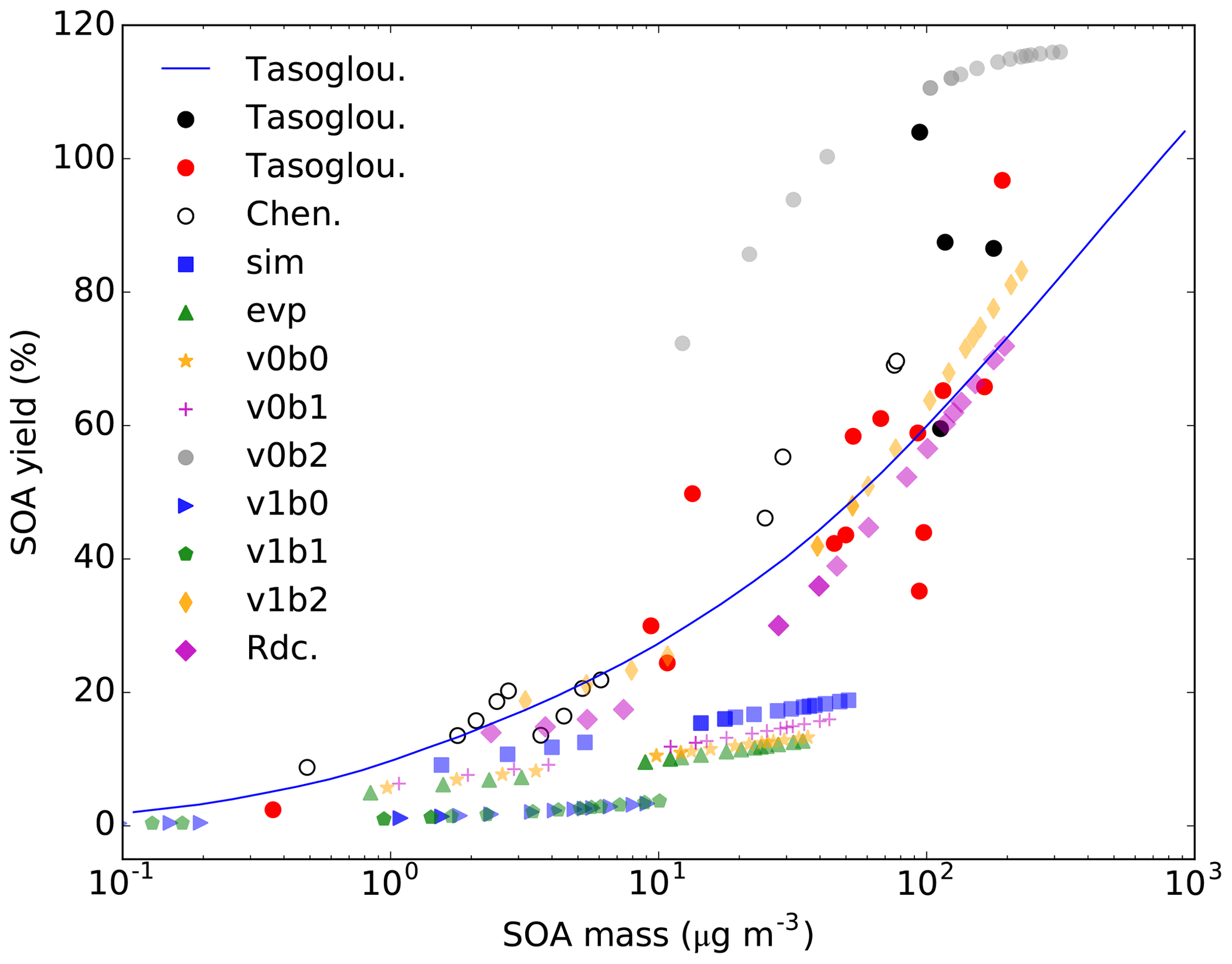
Figure A1The SOA yields versus the total SOA mass from the experimental data reported by Chen et al. (2012) and Tasoglou and Pandis (2015), simulated in SSH-aerosol with the MCM mechanism and different saturation vapor pressures methods (see the figure legend) and simulated with the Rdc. mechanism (purple diamonds). The Rdc. mechanism is trained from the MCM mechanism with the v1b2 method.
Table B1Species list of the Rdc. mechanism. Notice that the species in the reduced case may be different from the MCM species with identical names.
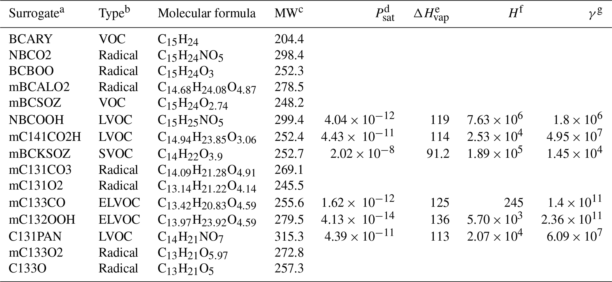
a Species with “m” are the new surrogates that merged multiple MCM BCARY species. b VOCs (stable gas-phase species) and radicals (unstable gas-phase species) are assumed not to undergo gas–particle partitioning. The volatility classes of condensable species are defined in Sect. 3. c Molar weight (g mol−1). The properties calculated for condensable substances only are as follows: d saturation vapor pressure at 298 K (atm), e enthalpy of vaporization (kJ mol−1), f Henry's law constant (mol L−1 atm−1), and g activity coefficient at infinite dilution in water.
Table B2Reaction list of the Rdc. mechanism.

a [H2O] is the concentration of H2O, [RO2] is the total concentration of the RO2 species pool, [O2] is the concentration of O2, and KFPAN is one of the complex rate coefficients from the MCM mechanism.
Table B3The new surrogates in the Rdc. mechanism and the corresponding lumped species in the original MCM mechanism. Notice that the Rdc. surrogates may also go through other reductions (i.e., jumping, replacement, and removal) that do not affect their molecular structures.
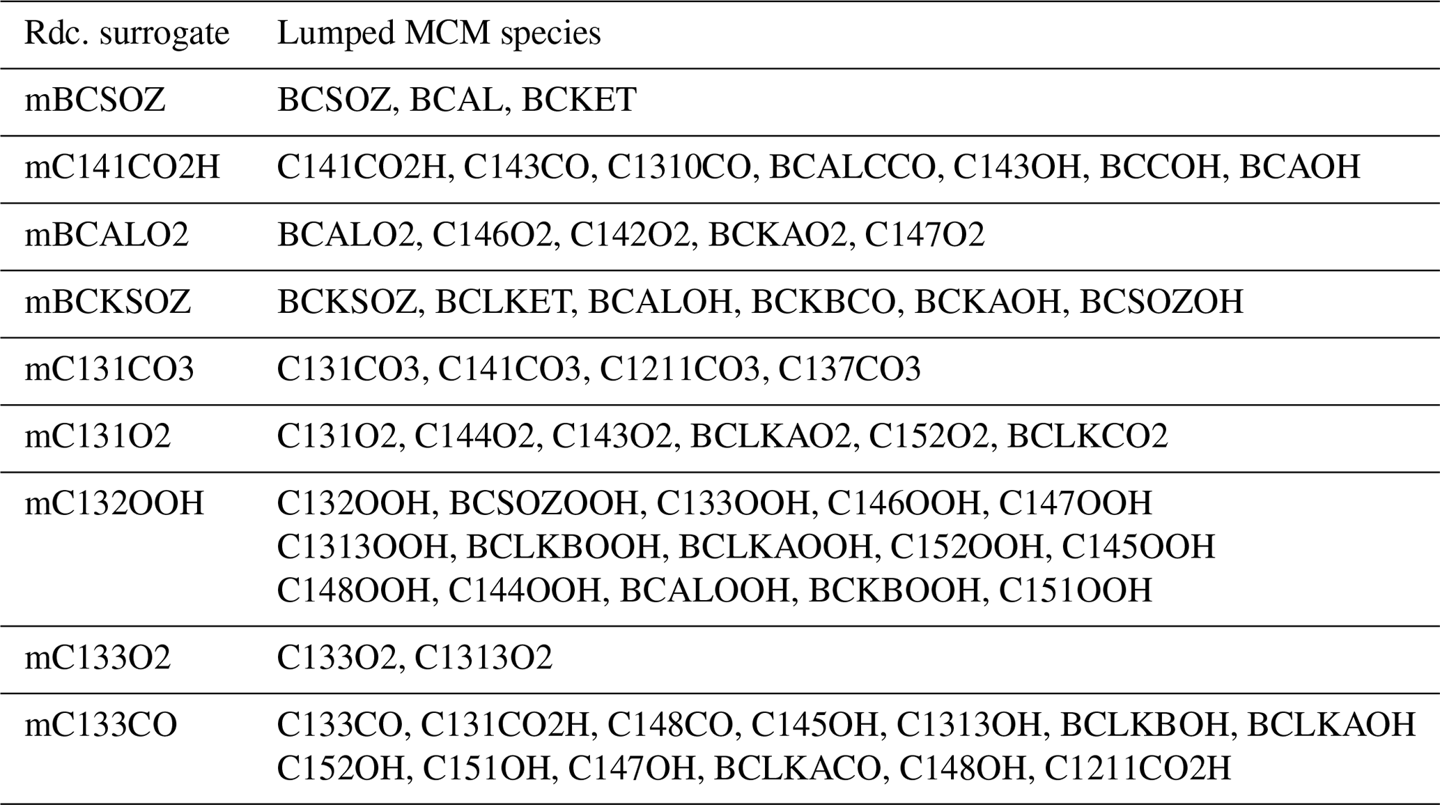
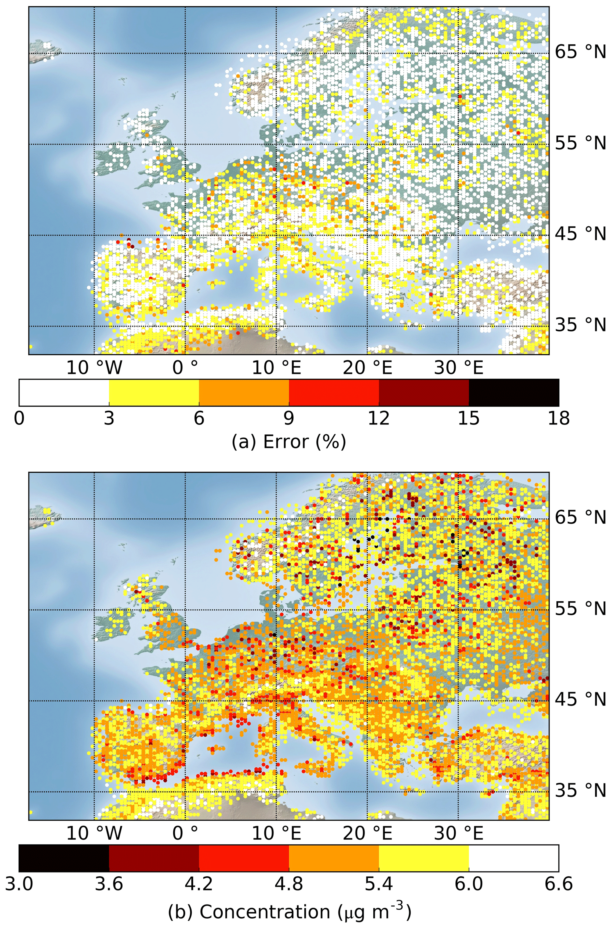
Figure B1Maps of the (a) error and (b) average SOA concentration of the testing results simulated using the Rdc. mechanism on all (i.e., 12 159) testing conditions.
C1 Additional examples of lumping
Besides the example shown in Sect. 2.2.3, two additional examples have been added from the BCARY reduction: one illustrates the lumping of two similar compounds formed by different reactions, and the other illustrates the lumping of two more distinct compounds. The first example is the MCM species C1313NO3 and C152NO3 (see Table C2). These two species come from different reactions. The molecular structures of both compounds are similar (they contain organic nitrates, aldehydes, and alcohols), but C152NO3 contains an additional carboxylic acid where C1313NO3 contains an aldehyde. The corresponding reactions before and after lumping are summarized in Table C2, where the new surrogate “mC1313NO3” is built from C1313NO3 with a weighting ratio of 83 % and C152NO3 with a weighting ratio of 17 %. As a result of this lumping, the average error increase under training conditions is 0.001 % (the tolerance is 0.01 %).
Table C1The computation of estimating chemical activity ratios used to display training dataset in Fig. 2.
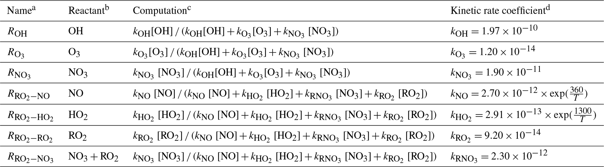
a Names of the reacting ratio of OH radical, O3, and NO3 radical reacted with BCARY () and of the reacting ratio of NO, HO2 radical, RO2 radical, and NO3 radical (in the presence of RO2) reacted with RO2 species (). b Reactions with those compounds are preferred when the corresponding reaction ratios are high. c [species_name] (e.g.,[OH]) is the monthly average concentration of oxidant concentrations extracted from CHIMERE. d Kinetic rate coefficients are provided by MCM, where kOH, , and are the kinetic rate coefficient of first-generation BCARY reaction with OH, O3, and NO3, respectively; kNO, , and are the simple rate coefficients KRO2NO, KRO2HO2, and KRO2NO3, respectively; and represents the self-reaction rate coefficients for the tertiary peroxy radicals (e.g., BCAO2 and BCCO2). T is temperature (K).
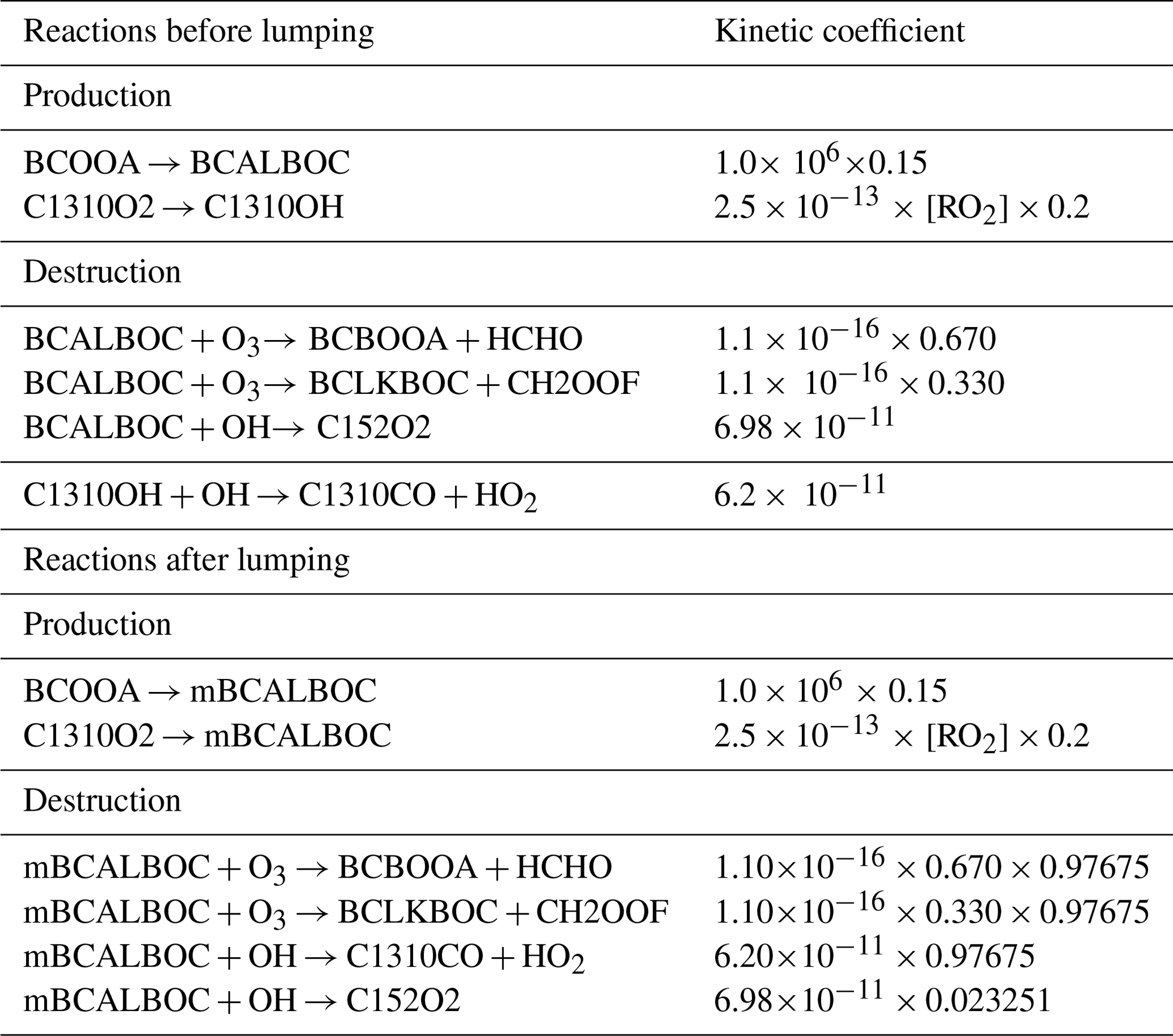
Another example of lumping is the MCM species BCALBOC and C1310OH (see Table C3). Unlike the previous example, these two species are more distinct. According to MCM, BCALBOC is generated through O3-initiated reactions, whereas C1310OH is generated through high-generation oxidations. There is less similarity in the structures or chemical reactions of the two molecules. MCM contains the OH reaction of BCALBOC as well as the O3 and OH reactions of C1310OH. However, this reduction was accepted because lumping them only increased the average error by 0.01 % under training conditions (the tolerance was 1 %). The new surrogate “mBCALBOC” is constructed from BCALBOC with a weighting ratio of 98 % and C1310OH with a weighting ratio of 2 %.
As C1310OH has a low weighting ratio, the lumping would be substituted by replacement (a special case of lumping), where the weighting ratio of BCALBOC is set to 100 % and the weighting ratio of C1310OH is set to 0 %. In this case, instead of forming a new surrogate, C1310OH is replaced by BCALBOC. In BCARY reduction, this type of replacement was not used, but it can be activated by the user by setting the weighting ratio threshold.
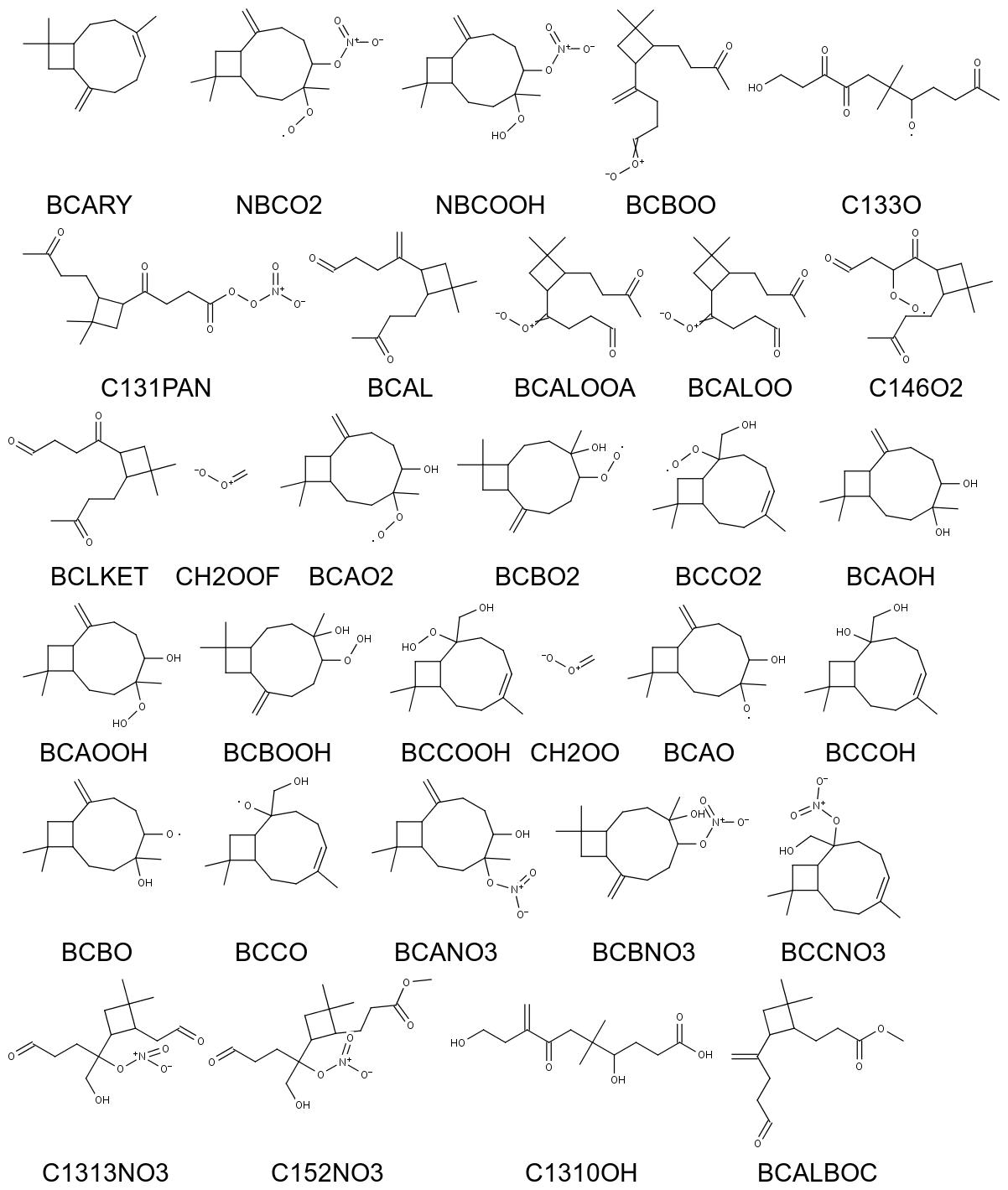
Figure C1Molecular structures of the MCM species that are mentioned in the paper. For more information, please visit the MCM website.
Table C2Reactions related to the reduction of the MCM species C1313NO3 and C152NO3 via lumping. The exact weighting ratio of C1313NO3 is 0.82945, and the exact weighting ratio of C152NO3 is 0.17055.

Table C3Reactions related to the reduction of the MCM species BCALBOC and C1310OH via lumping. The exact weighting ratio of BCALBOC is 0.97675, and the exact weighting ratio of C1310OH is 0.023251.
The source code for GENOA v1.0 is hosted on GitHub at https://github.com/tool-genoa/GENOA/tree/v1.0 (last access: 25 April 2022). The associated Zenodo DOI is https://doi.org/10.5281/zenodo.6482978 (Wang, 2022). The dataset that we used to run the BCARY MCM reduction is publicly available online on Zenodo: https://doi.org/10.5281/zenodo.6483088 (Wang et al., 2022).
The supplement related to this article is available online at: https://doi.org/10.5194/gmd-15-8957-2022-supplement.
ZW developed the model code and performed the simulations. ZW, FC, and KS designed the research and developed the methodology. ZW wrote the manuscript with contributions from FC and KS. FC and KS were responsible for funding acquisition.
The contact author has declared that none of the authors has any competing interests.
Publisher's note: Copernicus Publications remains neutral with regard to jurisdictional claims in published maps and institutional affiliations.
The authors would like to thank Youngseob Kim from CEREA for his help with using the SSH-aerosol model.
This research has been supported by INERIS and DIM QI2 (Air Quality Research Network on air quality in the Île-de-France region).
This paper was edited by Andrea Stenke and reviewed by William Carter and two anonymous referees.
Aumont, B., Szopa, S., and Madronich, S.: Modelling the evolution of organic carbon during its gas-phase tropospheric oxidation: development of an explicit model based on a self generating approach, Atmos. Chem. Phys., 5, 2497–2517, https://doi.org/10.5194/acp-5-2497-2005, 2005. a
Breysse, P. N., Delfino, R. J., Dominici, F., Elder, A. C. P., Frampton, M. W., Froines, J. R., Geyh, A. S., Godleski, J. J., Gold, D. R., Hopke, P. K., Koutrakis, P., Li, N., Oberdörster, G., Pinkerton, K. E., Samet, J. M., Utell, M. J., and Wexler, A. S.: US EPA particulate matter research centers: summary of research results for 2005–2011, Air Qual. Atmos. Health, 6, 333–355, https://doi.org/10.1007/s11869-012-0181-8, 2013. a
Carter, W. P.: Development of the SAPRC-07 chemical mechanism, Atmos. Environ., 44, 5324–5335, https://doi.org/10.1016/j.atmosenv.2010.01.026, 2010. a
Chen, Q., Li, Y. L., McKinney, K. A., Kuwata, M., and Martin, S. T.: Particle mass yield from β-caryophyllene ozonolysis, Atmos. Chem. Phys., 12, 3165–3179, https://doi.org/10.5194/acp-12-3165-2012, 2012. a, b, c, d
Compernolle, S., Ceulemans, K., and Müller, J.-F.: EVAPORATION: a new vapour pressure estimation methodfor organic molecules including non-additivity and intramolecular interactions, Atmos. Chem. Phys., 11, 9431–9450, https://doi.org/10.5194/acp-11-9431-2011, 2011. a
Couvidat, F. and Sartelet, K.: The Secondary Organic Aerosol Processor (SOAP v1.0) model: a unified model with different ranges of complexity based on the molecular surrogate approach, Geosci. Model Dev., 8, 1111–1138, https://doi.org/10.5194/gmd-8-1111-2015, 2015. a
Couvidat, F., Debry, E., Sartelet, K., and Seigneur, C.: A hydrophilic/hydrophobic organic (H2O) aerosol model: Development, evaluation and sensitivity analysis, J. Geophys. Res.-Atmos., 117, D10, https://doi.org/10.1029/2011JD017214, 2012. a
Derognat, C., Beekmann, M., Baeumle, M., Martin, D., and Schmidt, H.: Effect of biogenic volatile organic compound emissions on tropospheric chemistry during the Atmospheric Pollution Over the Paris Area (ESQUIF) campaign in the Ile-de-France region, J. Geophys. Res.-Atmos., 108, D17, https://doi.org/10.1029/2001JD001421, 2003. a
Donahue, N. M., Robinson, A. L., Stanier, C. O., and Pandis, S. N.: Coupled Partitioning, Dilution, and Chemical Aging of Semivolatile Organics, Environ. Sci. Technol., 40, 2635–2643, https://doi.org/10.1021/es052297c, 2006. a, b
Evtyugina, M., Pio, C., Nunes, T., Pinho, P., and Costa, C.: Photochemical ozone formation at Portugal West Coast under sea breeze conditions as assessed by master chemical mechanism model, Atmos. Environ., 41, 2171–2182, https://doi.org/10.1016/j.atmosenv.2006.10.059, 2007. a
Fredenslund, A., Jones, R. L., and Prausnitz, J. M.: Group-contribution estimation of activity coefficients in nonideal liquid mixtures, AIChE J., 21, 1086–1099, 1975. a
Gelencsér, A., May, B., Simpson, D., Sánchez-Ochoa, A., Kasper-Giebl, A., Puxbaum, H., Caseiro, A., Pio, C., and Legrand, M.: Source apportionment of PM2.5 organic aerosol over Europe: Primary/secondary, natural/anthropogenic, and fossil/biogenic origin, J. Geophys. Res.-Atmos., 112, D23, https://doi.org/10.1029/2006JD008094, 2007. a
Goliff, W., Stockwell, W., and Lawson, C.: The Regional Atmospheric Chemistry Mechanism, version 2, Atmos. Environ., 68, 174–185, https://doi.org/10.1016/j.atmosenv.2012.11.038, 2013. a
Griffin, R. J., Nguyen, K., Dabdub, D., and Seinfeld, J. H.: A Coupled Hydrophobic-Hydrophilic Model for Predicting Secondary Organic Aerosol Formation, J. Atmos. Chem., 44, 171–190, https://doi.org/10.1023/A:1022436813699, 2003. a
Hallquist, M., Wenger, J. C., Baltensperger, U., Rudich, Y., Simpson, D., Claeys, M., Dommen, J., Donahue, N. M., George, C., Goldstein, A. H., Hamilton, J. F., Herrmann, H., Hoffmann, T., Iinuma, Y., Jang, M., Jenkin, M. E., Jimenez, J. L., Kiendler-Scharr, A., Maenhaut, W., McFiggans, G., Mentel, Th. F., Monod, A., Prévôt, A. S. H., Seinfeld, J. H., Surratt, J. D., Szmigielski, R., and Wildt, J.: The formation, properties and impact of secondary organic aerosol: current and emerging issues, Atmos. Chem. Phys., 9, 5155–5236, https://doi.org/10.5194/acp-9-5155-2009, 2009. a
Hellén, H., Schallhart, S., Praplan, A. P., Tykkä, T., Aurela, M., Lohila, A., and Hakola, H.: Sesquiterpenes dominate monoterpenes in northern wetland emissions, Atmos. Chem. Phys., 20, 7021–7034, https://doi.org/10.5194/acp-20-7021-2020, 2020. a
Huang, X., Ding, A., Gao, J., Zheng, B., Zhou, D., Qi, X., Tang, R., Wang, J., Ren, C., Nie, W., Chi, X., Xu, Z., Chen, L., Li, Y., Che, F., Pang, N., Wang, H., Tong, D., Qin, W., Cheng, W., Liu, W., Fu, Q., Liu, B., Chai, F., Davis, S. J., Zhang, Q., and He, K.: Enhanced secondary pollution offset reduction of primary emissions during COVID-19 lockdown in China, Natl. Sci. Rev., 8, 2, https://doi.org/10.1093/nsr/nwaa137, 2020. a
Jenkin, M., Watson, L., Utembe, S., and Shallcross, D.: A Common Representative Intermediates (CRI) mechanism for VOC degradation. Part 1: Gas phase mechanism development, Atmos. Environ., 42, 7185–7195, https://doi.org/10.1016/j.atmosenv.2008.07.028, 2008. a
Jenkin, M. E., Saunders, S. M., and Pilling, M. J.: The tropospheric degradation of volatile organic compounds: a protocol for mechanism development, Atmos. Environ., 31, 81–104, https://doi.org/10.1016/S1352-2310(96)00105-7, 1997. a
Jenkin, M. E., Wyche, K. P., Evans, C. J., Carr, T., Monks, P. S., Alfarra, M. R., Barley, M. H., McFiggans, G. B., Young, J. C., and Rickard, A. R.: Development and chamber evaluation of the MCM v3.2 degradation scheme for β-caryophyllene, Atmos. Chem. Phys., 12, 5275–5308, https://doi.org/10.5194/acp-12-5275-2012, 2012. a, b, c, d
Joback, K. G. and Reid, R. C.: Estimation of pure-component properties from group-contributions, Chem. Eng. Comm., 57, 233–243, https://doi.org/10.1080/00986448708960487, 1987. a, b, c
Kanakidou, M., Seinfeld, J. H., Pandis, S. N., Barnes, I., Dentener, F. J., Facchini, M. C., Van Dingenen, R., Ervens, B., Nenes, A., Nielsen, C. J., Swietlicki, E., Putaud, J. P., Balkanski, Y., Fuzzi, S., Horth, J., Moortgat, G. K., Winterhalter, R., Myhre, C. E. L., Tsigaridis, K., Vignati, E., Stephanou, E. G., and Wilson, J.: Organic aerosol and global climate modelling: a review, Atmos. Chem. Phys., 5, 1053–1123, https://doi.org/10.5194/acp-5-1053-2005, 2005. a
Khan, M., Jenkin, M., Foulds, A., Derwent, R., Percival, C., and Shallcross, D.: A modeling study of secondary organic aerosol formation from sesquiterpenes using the STOCHEM global chemistry and transport model, J. Geophys. Res.-Atmos., 122, 4426–4439, https://doi.org/10.1002/2016JD026415, 2017. a, b
Kim, Y., Couvidat, F., Sartelet, K., and Seigneur, C.: Comparison of Different Gas-Phase Mechanisms and Aerosol Modules for Simulating Particulate Matter Formation, J. Air Waste Manag. Assoc., 61, 1218–1226, https://doi.org/10.1080/10473289.2011.603999, 2011. a
Kim, Y., Sartelet, K., and Couvidat, F.: Modeling the effect of non-ideality, dynamic mass transfer and viscosity on SOA formation in a 3-D air quality model, Atmos. Chem. Phys., 19, 1241–1261, https://doi.org/10.5194/acp-19-1241-2019, 2019. a
Lannuque, V., Camredon, M., Couvidat, F., Hodzic, A., Valorso, R., Madronich, S., Bessagnet, B., and Aumont, B.: Exploration of the influence of environmental conditions on secondary organic aerosol formation and organic species properties using explicit simulations: development of the VBS-GECKO parameterization, Atmos. Chem. Phys., 18, 13411–13428, https://doi.org/10.5194/acp-18-13411-2018, 2018. a
Lanzafame, G. M., Bessagnet, B., Srivastava, D., Jaffrezo, J. L., Favez, O., Albinet, A., and Couvidat, F.: Modelling aerosol molecular markers in a 3D air quality model: Focus on anthropogenic organic markers, Sci. Total Environ., 835, 155360, https://doi.org/10.1016/j.scitotenv.2022.155360, 2022. a
Li, J., Cleveland, M., Ziemba, L. D., Griffin, R. J., Barsanti, K. C., Pankow, J. F., and Ying, Q.: Modeling regional secondary organic aerosol using the Master Chemical Mechanism, Atmos. Environ., 102, 52–61, https://doi.org/10.1016/j.atmosenv.2014.11.054, 2015. a
McNeill, V. F.: Atmospheric Aerosols: Clouds, Chemistry, and Climate, Annual Rev. Chem. Biomol. Eng., 8, 427–444, https://doi.org/10.1146/annurev-chembioeng-060816-101538, 2017. a
Myrdal, P. B. and Yalkowsky, S. H.: Estimating Pure Component Vapor Pressures of Complex Organic Molecules, Ind. Eng. Chem. Res., 36, 2494–2499, https://doi.org/10.1021/ie950242l, 1997. a
Nannoolal, Y., Rarey, J., Ramjugernath, D., and Cordes, W.: Estimation of pure component properties: Part 1. Estimation of the normal boiling point of non-electrolyte organic compounds via group contributions and group interactions, Fluid Phase Equilibr., 226, 45–63, https://doi.org/10.1016/j.fluid.2004.09.001, 2004. a
Nannoolal, Y., Rarey, J., and Ramjugernath, D.: Estimation of pure component properties: Part 3. Estimation of the vapor pressure of non-electrolyte organic compounds via group contributions and group interactions, Fluid Phase Equilibr., 269, 117–133, https://doi.org/10.1016/j.fluid.2008.04.020, 2008. a, b, c
Odum, J. R., Hoffmann, T., Bowman, F., Collins, D., Flagan, R. C., and Seinfeld, J. H.: Gas/Particle Partitioning and Secondary Organic Aerosol Yields, Environ. Sci. Technol., 30, 2580–2585, https://doi.org/10.1021/es950943+, 1996. a
Pankow, J. F. and Asher, W. E.: SIMPOL.1: a simple group contribution method for predicting vapor pressures and enthalpies of vaporization of multifunctional organic compounds, Atmos. Chem. Phys., 8, 2773–2796, https://doi.org/10.5194/acp-8-2773-2008, 2008. a
Porter, W. C., Jimenez, J. L., and Barsanti, K. C.: Quantifying atmospheric parameter ranges for ambient secondary organic aerosol formation, ACS Earth Space Chem., 5, 2380–2397, https://doi.org/10.1021/acsearthspacechem.1c00090, 2021. a
Pun, B. K., Seigneur, C., and Lohman, K.: Modeling Secondary Organic Aerosol Formation via Multiphase Partitioning with Molecular Data, Environ. Sci. Technol., 40, 4722–4731, https://doi.org/10.1021/es0522736, 2006. a
Ramanathan, V., Crutzen, P. J., Kiehl, J., and Rosenfeld, D.: Aerosols, climate, and the hydrological cycle, Science, 294, 2119–2124, https://doi.org/10.1126/science.1064034, 2001. a
Sartelet, K., Couvidat, F., Wang, Z., Flageul, C., and Kim, Y.: SSH-Aerosol v1. 1: A Modular Box Model to Simulate the Evolution of Primary and Secondary Aerosols, Atmosphere, 11, 525, https://doi.org/10.3390/atmos11050525, 2020. a, b
Sarwar, G., Luecken, D., Yarwood, G., Whitten, G. Z., and Carter, W. P. L.: Impact of an Updated Carbon Bond Mechanism on Predictions from the CMAQ Modeling System: Preliminary Assessment, J. Appl. Meteorol., 47, 3–14, https://doi.org/10.1175/2007JAMC1393.1, 2008. a
Saunders, S. M., Jenkin, M. E., Derwent, R. G., and Pilling, M. J.: Protocol for the development of the Master Chemical Mechanism, MCM v3 (Part A): tropospheric degradation of non-aromatic volatile organic compounds, Atmos. Chem. Phys., 3, 161–180, https://doi.org/10.5194/acp-3-161-2003, 2003. a
Schwarze, P. E., Øvrevik, J., Låg, M., Refsnes, M., Nafstad, P., Hetland, R. B., and Dybing, E.: Particulate matter properties and health effects: consistency of epidemiological and toxicological studies, Hum. Exp. Toxicol., 25, 559–579, https://doi.org/10.1177/096032706072520, 2006. a
Seinfeld, J. H. and Pandis, S. N.: Atmospheric chemistry and physics: from air pollution to climate change, John Wiley & Sons, ISBN 978-1-119-22117-3, 2016. a, b
Sommariva, R., Trainer, M., de Gouw, J. A., Roberts, J. M., Warneke, C., Atlas, E., Flocke, F., Goldan, P. D., Kuster, W. C., Swanson, A. L., and Fehsenfeld, F. C.: A study of organic nitrates formation in an urban plume using a Master Chemical Mechanism, Atmos. Environ., 42, 5771–5786, https://doi.org/10.1016/j.atmosenv.2007.12.031, 2008. a
Stein, S. E. and Brown, R. L.: Estimation of normal boiling points from group contributions, J. Chem. Inf. Comput. Sci., 34, 581–587, https://doi.org/10.1021/ci00019a016, 1994. a
Szopa, S., Aumont, B., and Madronich, S.: Assessment of the reduction methods used to develop chemical schemes: building of a new chemical scheme for VOC oxidation suited to three-dimensional multiscale HOx-NOx-VOC chemistry simulations, Atmos. Chem. Phys., 5, 2519–2538, https://doi.org/10.5194/acp-5-2519-2005, 2005. a
Tasoglou, A. and Pandis, S. N.: Formation and chemical aging of secondary organic aerosol during the β-caryophyllene oxidation, Atmos. Chem. Phys., 15, 6035–6046, https://doi.org/10.5194/acp-15-6035-2015, 2015. a, b, c, d, e
Topping, D., Barley, M., Bane, M. K., Higham, N., Aumont, B., Dingle, N., and McFiggans, G.: UManSysProp v1.0: an online and open-source facility for molecular property prediction and atmospheric aerosol calculations, Geosci. Model Dev., 9, 899–914, https://doi.org/10.5194/gmd-9-899-2016, 2016. a
Wang, Z.: tool-genoa/GENOA: GENOA v1.0 (v1.0), Zenodo [code], https://doi.org/10.5281/zenodo.6482978, 2022. a
Wang, Z., Couvidat, F., and Sartelet, K.: The electronic supplement of the article “GENerator of reduced Organic Aerosol mechanism (GENOA v1.0): An automatic generation tool of semi-explicit mechanisms” (v1.1), Zenodo [data set], https://doi.org/10.5281/zenodo.6483088, 2022. a
Watson, L., Shallcross, D., Utembe, S., and Jenkin, M.: A Common Representative Intermediates (CRI) mechanism for VOC degradation. Part 2: Gas phase mechanism reduction, Atmos. Environ., 42, 7196–7204, https://doi.org/10.1016/j.atmosenv.2008.07.034, 2008. a
Xavier, C., Rusanen, A., Zhou, P., Dean, C., Pichelstorfer, L., Roldin, P., and Boy, M.: Aerosol mass yields of selected biogenic volatile organic compounds – a theoretical study with nearly explicit gas-phase chemistry, Atmos. Chem. Phys., 19, 13741–13758, https://doi.org/10.5194/acp-19-13741-2019, 2019. a
Ying, Q. and Li, J.: Implementation and initial application of the near-explicit Master Chemical Mechanism in the 3D Community Multiscale Air Quality (CMAQ) model, Atmos. Environ., 45, 3244–3256, https://doi.org/10.1016/j.atmosenv.2011.03.043, 2011. a
Zhang, Y., Xue, L., Li, H., Chen, T., Mu, J., Dong, C., Sun, L., Liu, H., Zhao, Y., Wu, D., Wang, X., and Wang, W.: Source Apportionment of Regional Ozone Pollution Observed at Mount Tai, North China: Application of Lagrangian Photochemical Trajectory Model and Implications for Control Policy, J. Geophys. Res.-Atmos., 126, e2020JD033519, https://doi.org/10.1029/2020JD033519, 2021. a
Zuend, A., Marcolli, C., Luo, B. P., and Peter, T.: A thermodynamic model of mixed organic-inorganic aerosols to predict activity coefficients, Atmos. Chem. Phys., 8, 4559–4593, https://doi.org/10.5194/acp-8-4559-2008, 2008. a
- Abstract
- Introduction
- Model development
- Application to the β-caryophyllene mechanism
- Conclusions
- Appendix A: The computation of saturation vapor pressure of BCARY SVOCs
- Appendix B: An overview of the Rdc. mechanism
- Appendix C: Information related to the reduction
- Code and data availability
- Author contributions
- Competing interests
- Disclaimer
- Acknowledgements
- Financial support
- Review statement
- References
- Supplement