the Creative Commons Attribution 4.0 License.
the Creative Commons Attribution 4.0 License.
 | 25 Nov 2022
The Baltic Sea Model Intercomparison Project (BMIP) – a platform for model development, evaluation, and uncertainty assessment
Matthias Gröger
Manja Placke
H. E. Markus Meier
Florian Börgel
Sandra-Esther Brunnabend
Cyril Dutheil
Ulf Gräwe
Magnus Hieronymus
Thomas Neumann
Hagen Radtke
Semjon Schimanke
Germo Väli
While advanced computational capabilities have enabled the development of complex ocean general circulation models (OGCMs) for marginal seas, systematic comparisons of regional ocean models and their setups are still rare. The Baltic Sea Model Intercomparison Project (BMIP), introduced herein, was therefore established as a platform for the scientific analysis and systematic comparison of Baltic Sea models. The inclusion of a physically consistent regional reanalysis data set for the period 1961–2018 allows for standardized meteorological forcing and river runoff. Protocols to harmonize model outputs and analyses are provided as well.
An analysis of six simulations performed with four regional OGCMs differing in their resolution, grid coordinates, and numerical methods was carried out to explore intermodel differences despite harmonized forcing. Uncertainties in the modeled surface temperatures were shown to be larger at extreme than at moderate temperatures. In addition, a roughly linear increase in the temperature spread with increasing water depth was determined and indicated larger uncertainties in the near-bottom layer. On the seasonal scale, the model spread was larger in summer than in winter, likely due to differences in the models' thermocline dynamics. In winter, stronger air–sea heat fluxes and vigorous convective and wind mixing reduced the intermodel spread. Uncertainties were likewise reduced near the coasts, where the impact of meteorological forcing was stronger. The uncertainties were highest in the Bothnian Sea and Bothnian Bay, attributable to the differences between the models in the seasonal cycles of sea ice triggered by the ice–albedo feedback. However, despite the large spreads in the mean climatologies, high interannual correlations between the sea surface temperatures (SSTs) of all models and data derived from a satellite product were determined. The exceptions were the Bothnian Sea and Bothnian Bay, where the correlation dropped significantly, likely related to the effect of sea ice on air–sea heat exchange.
The spread of water salinity across the models is generally larger compared to water temperature, which is most obvious in the long-term time series of deepwater salinity. The inflow dynamics of saline water from the North Sea is covered well by most models, but the magnitude, as inferred from salinity, differs as much as the simulated mean salinity of deepwater.
Marine heat waves (MHWs), coastal upwelling, and stratification were also assessed. In all models, MHWs were more frequent in shallow areas and in regions with seasonal ice cover. An increase in the frequency (regionally varying between ∼50 % and 250 %) and duration (50 %–150 %) of MHWs during the last 3 decades in all models was found as well. The uncertainties were highest in the Bothnian Bay, likely due to the different trends in sea ice presence. All but one of the analyzed models overestimated upwelling frequencies along the Swedish coast, the Gulf of Finland, and around Gotland, while they underestimated upwelling in the Gulf of Riga. The onset and seasonal cycle of thermal stratification likewise differed among the models. Compared to observation-based estimates, in all models the thermocline in early spring was too deep, whereas a good match was obtained in June when the thermocline intensifies.
- Article
(15925 KB) - Full-text XML
-
Supplement
(40921 KB) - BibTeX
- EndNote


Coordinated model experiments are common practice in global ocean model modeling, as exemplified by the ocean model intercomparison project (OMIP; Griffies et al., 2016) which seeks to identify systematic model biases and to address intermodel differences between participating models. However, parallel efforts in modeling regional seas are still rare and have mostly focused on wider open-ocean regions, such as the Arctic (e.g., the Arctic Ocean Model Comparison Project; https://web.whoi.edu/famos/, last access: 16 November 2022) and the North Atlantic (Barnard et al., 1997). Shelf seas have yet to be systematically studied despite their high economic importance. For the shallow Baltic Sea and North Sea, only a few non-systematic studies have included intermodel comparisons (e.g., Myrberg et al., 2010; Eilola et al., 2011; Placke et al., 2018; Pätsch et al., 2017). Hence, in the following, we introduce the Baltic Sea Model Intercomparison Project (BMIP). The Baltic Sea is an estuarine sea on the NW European shelf and is an important factor in the economies of nine European countries (Russia, Finland, Estonia, Latvia, Lithuania, Poland, Germany, Denmark, and Sweden). However, unlike other marginal seas, the Baltic Sea has become highly eutrophic due to agricultural and industrial inputs from the hydrological catchment area. Furthermore, the impact of climate warming is expected to be high (e.g., Meier et al., 2018, 2019b, 2021a, b, 2022; Saraiva et al., 2019; Gröger et al., 2019, 2021a, b, 2022; Dieterich et al., 2019; Wahlström et al., 2020, 2022).

Figure 1(a) Bathymetry of the Baltic Sea. Red boxes indicate the positions of the Swedish stations used in wind and temperature analyses (see Sect. S1 in the Supplement). (b) Basin division for the Baltic Sea, according to Meier et al. (1999). Red circles indicate stations used for model vs. data comparisons.
The Baltic Sea is among the most complicated regions of the world ocean, given the complex bathymetry with several subbasins (Fig. 1) and the limited water exchange between them. The estuarine character of the Baltic Sea is due to sporadic saltwater intrusions from the North Sea, which are the product of complex overflows occurring across the Great Belt and the Sound region (Fig. 1), and lead to a permanent halocline between 60 and 80 m depth (Väli et al., 2013). The long history of oceanographic research in the Baltic Sea has resulted in numerous, very diverse models, ranging from simple box models (e.g., Knudsen, 1900; Welander, 1974) to process-oriented models (e.g., Stigebrandt, 1983, 1987; Omstedt, 1990; Omstedt and Axell, 2003) and, later, to general circulation models (GCMs). The latter include advanced methods for the vertical and horizontal discretization of partial differential equations for momentum, energy, and mass conservation at fine-resolution grids and for various empirical subgrid-scale parameterizations (e.g., Meier et al., 1999; Meier, 2001; Myrberg et al., 2010; Hordoir et al., 2019). An overview of the history of regional climate modeling for the Baltic Sea and its surrounding catchment area, since the 1990s, using GCMs was provided by Meier and Saraiva (2020).
A first initiative to systematically investigate physical properties of the Baltic Sea using multiple models focused on the Gulf of Finland (Myrberg et al., 2010). The authors compared six different 3D hydrodynamical models which were driven by the same atmospheric forcing, initial conditions, and the same model grid with a resolution of 4×2 min. The study identified common difficulties in representing the mixed-layer dynamics resulting in biases in vertical temperature and salinity profiles. The authors emphasized the need for higher-resolution and more advanced mixing schemes and accurate inputs of river discharge. However, the simulations comprised only the summer–autumn of 1996 and, thus, did not allow for assessing the long-term climate variability.
The, as yet, largest but most uncoordinated ensemble of scenario simulations for the Baltic Sea was analyzed by Meier et al. (2018), and the uncertainties in these projections were discussed in a subsequent publication (Meier et al., 2019a). As the model simulations during the historical period differed from the observations, and with mismatches between ocean models attributed to differences in atmospheric forcing, it was concluded that model performance must be rigorously assessed to improve future projections and to reduce the spread among models. Accordingly, Placke et al. (2018) examined water mass circulation in different hydrodynamical models for the 30-year period covering 1970–1999 and compared the results with reanalysis data. They found that a substantial portion of the intermodel differences could be explained simply by the different wind forcings and by the riverine freshwater inputs used to force the models. In addition, they showed that, compared with observations, newer ocean circulation models did not always perform better than the first Baltic Sea models, which were developed 20 years ago.
During recent decades, more powerful computational facilities have allowed the development of increasingly complex numerical methods (e.g., horizontal advection schemes, adaptive vertical coordinates, and unstructured grids). In addition, advanced schemes for subgrid-scale parameterizations (e.g., horizontal and vertical turbulence) have been developed. In parallel, the amount of available forcing data describing river discharge and the atmospheric boundary layer has also increased. However, comparisons of the internal process formulations of these different models require a harmonization of the experimental design (spinup, initialization, open lateral boundary conditions, atmospheric forcing, and river discharge). Moreover, despite advancements in model development, no new attempts have been made to systematically compare and validate Baltic Sea models since the studies of Myrberg et al. (2010) and Eilola et al. (2011).
The BMIP can close this gap by providing a coordinated framework for an experimental design, a model output, and the analyses of model results. Among the aims of the project are the development and provision of driving data for the most important forcings of Baltic Sea models, i.e., atmospheric boundary data, river discharge, and lateral boundary data. Furthermore, the BMIP includes recommendations for model initialization and spinup. The overall goal of this community effort is to improve the quality of Baltic Sea models, especially for climate variability, and, in turn, climate impact research.
Thus, in this first BMIP paper, the focus is on the models used for climate simulations, i.e., models that can be integrated over several decades with reasonable resources. However, the BMIP also considers models that were developed for operational short-term marine forecasts (e.g., sea level and sea ice), such as the HIROMB-BOOS ocean circulation model (HBM) from the Danish Meteorological Institute (Berg and Weismann Poulsen, 2012). Over longer timescales, the performance of these models can be expected to deteriorate when they are driven with data assimilation but evolve freely. Consequently, these models have rarely been validated with respect to their long-term performance, such as in multidecadal transient simulations. Finally, the BMIP also includes model setups with horizontal resolutions in the range of a few tens of meters to ∼200 m, as they allow the resolution of submesoscale dynamics and mesoscale eddy fields (Väli et al., 2017, 2018; Zhurbas et al., 2019b; Onken et al., 2020).
The paper is organized as follows. Section 2 provides a description of the forcing data sets to be used in the BMIP and outlines the protocol to set up a BMIP run. Section 3 assesses the results of six hindcast simulations from four different model platforms. Section 4 compares topical case studies for marine heat waves (MHWs) coastal upwellings, and water stratification. Section 5 discusses aspects of ultra-high-resolution modeling (∼250 m) within BMIP. A summary and the main conclusions constitute Sect. 6.
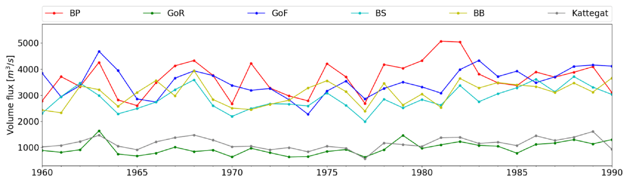
Figure 2Annual mean freshwater input to different subbasins of the Baltic Sea from the BMIP runoff forcing for the years 1960–1990. Figure adopted from Väli et al. (2019). BP is Baltic proper, GoR is the Gulf of Riga, GoF is the Gulf of Finland, BS is the Bothnian Sea, and BB is Bothnian Bay.
2.1 Forcing data
Runoff
Since runoff is a key parameter for most brackish marginal seas, the availability of physically consistent multidecadal discharge time series are a prerequisite for climate modeling in the Baltic Sea. As there are no homogeneous river discharge data sets for the entire period (1961–2018) available, and as the last years are only covered by an E-HYPE (Europe HypeWeb) model forecast product, a new homogeneous runoff product was produced within the BMIP project.
The homogeneous data set describing freshwater input to the Baltic Sea was produced (Fig. 2) with the aim of forcing each of the Baltic Sea models with identical runoff. The new data set is based on the runoff hindcast obtained with the pan-European hydrology model E-HYPE (Lindström et al., 2010) and forced by meteorological ERA-Interim data (Dee et al., 2011) that were downscaled using the regional atmosphere model, RCA3 (Samuelsson et al., 2011), for the period 1979–2012. For the period 2012–2018, an E-HYPE model forecast product (Donnelly et al., 2016) was used. For the early period (1961–1978), climatological runoff data from 1979 to 2008 had to be used, but these data were scaled by the annual mean values for the period 1961–1978, as reported by Bergström and Carlsson (1994). For the Neva River, the largest river in the eastern Gulf of Finland, daily observations for 1961–2016 were provided by the Russian State Hydrological Institute (Sergei Zhuravlev, personal communication, 2019). For detailed information on the runoff data set, the reader is referred to Väli et al. (2019).
The European Regional Reanalysis UERRA (version 1.0)
The regional reanalysis data set UERRA-HARMONIE was chosen as the atmospheric forcing for the present OMIP as it provides a physically consistent data set over almost 60 years and thus fits the requirements for transient multidecadal simulations. The UERRA-HARMONIE reanalysis system was developed within the FP7 project UERRA (Uncertainties in Ensembles of Regional Re-Analyses; http://www.uerra.eu/, last access: 16 November 2022). The data set was initially produced in the UERRA project and then carried over to the Copernicus Climate Change Service (C3S; https://climate.copernicus.eu/copernicus-regional-reanalysis-europe, last access: 16 November 2022). UERRA-HARMONIE is a long-term, high-quality, high-resolution regional reanalysis that includes many essential climate variables. Data on air temperature, pressure, humidity, wind speed and direction, cloud cover, precipitation, albedo, surface heat fluxes, and radiation fluxes are available for the period of January 1961 through July 2019, which is long enough for climatological analyses. We note that no correction was applied to the radiation parameters. Precipitation turned out to be sensitive to spinup effects after the data assimilation. Therefore, we subtract the 12 h forecast precipitation from the 24 h forecast to avoid the model spinup. UERRA-HARMONIE has a horizontal resolution of 11 km, with analyses carried out at 00:00, 06:00, 12:00, and 18:00 UTC; data from the forecast model with hourly resolution are also provided. UERRA-HARMONIE is available via Copernicus Climate Data Store (CDS; https://cds.climate.copernicus.eu/#!/home, last access: 16 November 2022). The parameters needed for the forcing of the ocean models belong to the category of single-level data and can be directly accessed at https://cds.climate.copernicus.eu/cdsapp#!/dataset/reanalysis-uerra-europe-single-levels?tab=overview (last access: 16 November 2022).
Potential shortcomings of the data set are related to parameters based on the forecast model only, i.e., parameters which are not assimilated. A prominent example here is the total precipitation. The surface water budget in UERRA-HARMONIE is not closed, and the total precipitation is overestimated, and therefore it is reduced by 20 % for BMIP. The UERRA-HARMONIE cloudiness was corrupted in the post-processing step before archiving. Unfortunately, a cloud cover of 100 % was archived as cloud free (0 %). Therefore, it is suggested that coastDat-2 cloudiness be used in the BMIP context. No other corrections were made to the data set.
The data are freely available upon registration and acceptance of the license. Within the Copernicus User Learning Services (ULS) GitHub (https://github.com/UserLearningServices-C3S/regionalreanalysis-UERRA, last access: 16 November 2022), an example of data access and preparation is provided using the NEMO-Nordic model (Hordoir et al., 2019). Shortcomings in UERRA-HARMONIE, e.g., for precipitation or cloudiness, are explained in the instruction file on the BMIP website (https://www.baltic.earth/working_groups/model_intercomparison/index.php.en, last access: 16 November 2022), which also offers solutions on how to deal with those parameters. Both a brief assessment of the atmospheric data with respect to observations and the ERA5 reanalysis data are available in Sect. S1 in the Supplement.
2.2 Ocean models
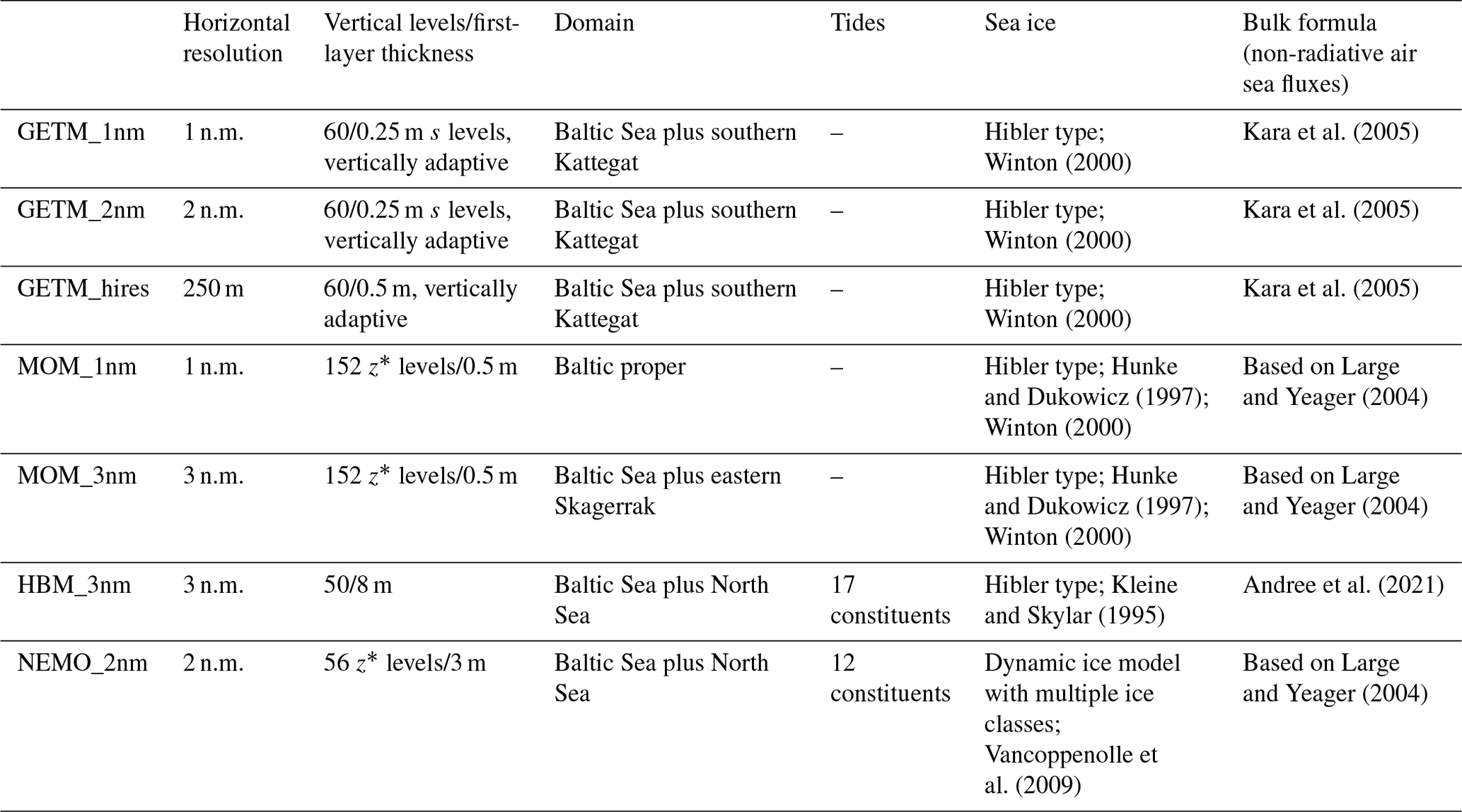
Six configurations based on four different model platforms (GETM, MOM, HBM, and NEMO) were assessed in this study, with a focus on the models' capability to describe long-term climatologies and dynamics. While the GETM (General Estuarine Transport Model), MOM (Modular Ocean Model), and NEMO (Nucleus for European Modeling of the Ocean) were designed for free long-term integrations of multiple decades, the HBM is primarily used for short-term operational services and was thus designed to mainly operate with data assimilation techniques. In the BMIP, it was run for the first time in free mode.
Table 1 provides information on the model setups assessed in this study. The GETM_1nm and GETM_2nm domains cover the Baltic Sea, including the Kattegat region, while the two MOM domains also include parts of the Skagerrak. Both the NEMO and HBM domains encompass the Baltic and the North Sea, for which they also use tidal forcing on the lateral boundary condition. The horizontal resolution of these models is between 1 and 3 n.m. (nautical miles). GETM_hires was integrated only for a few months, as it is too expensive for multidecadal simulations. The NEMO_2nm model incorporates a multiclass dynamical ice model, while the other models include simpler Hibler-type models. The model setups vary strongly in their vertical discretization. Thus, while the GETM uses 60 vertical adaptive terrains following s coordinates (Hofmeister et al., 2010), the other models have z* coordinates that, at every time step, are rescaled to the actual sea surface height. Surface layer thicknesses ranges from 0.25 (GETM) to 8 m (HBM). All models use the radiative fluxes (downward longwave and downward shortwave) provided by the BMIP forcing but differ in their calculation of momentum flux (wind stress), sensible and latent surface heat fluxes, and in their upward longwave radiation, all of which were estimated using different bulk formulas from the other surface fields provided by the BMIP.
While the BMIP provides time series of runoff, the implementation may differ between models due to technical design and model setup (e.g., horizontal and vertical resolution). For this study, runoff was implemented along the coasts as follows:
-
HBM and MOM runoff is added to one coastal grid cell in the top layer
-
GETM is always in the top cell
-
discharge of <500 m3 s−1 is for the one cell discharge near the coast
-
discharge of <1000 m3 s−1 is spread evenly over two horizontal cells near the coast
-
discharge of >1000 m3 s−1 is spread evenly over three horizontal cells near the coast
-
NEMO is one cell discharge near the coast and distributed over the whole water column.
As HBM is an operational setup, it is straight forward, for its implementation, to utilize the respective runoff data set for this purpose. Thus, HBM differs from the other models with respect to the used runoff data. Nonetheless, the hydrological data set used for HBM in this study is derived from the same source as for other models, i.e., E-HYPE forecasts (Donnelly et al., 2016), but did not undergo the harmonization procedure during the compilation of the official BMIP runoff data set. All other forcing data are exactly the same as for the other models.
A short description of each model, along with further references regarding details of the respective physics, can be found in Sect. S2.
Table 1Overview of the models used in this study (nm is nautical miles).
2.3 The BMIP protocol version 1.0
The BMIP was invoked to establish atmospheric and hydrological forcing data and to develop best practices in the setup of climate simulations for the Baltic Sea. Discussions within the international project group have addressed the ability of state-of-the-art ocean general circulation models to sufficiently represent climate-relevant ocean processes and the required grid resolution and improve parameterizations specific for the Baltic Sea's physics (i.e., the sea's variable topography, estuarine circulation due to excessive freshwater input, and the impact of tides), and (in a second phase) marine biogeochemistry. The aim of BMIP is to improve the performance of Baltic Sea simulations, for both past and future climates, and to foster international scientific collaboration on ocean climate model development and setup.
The forcing data and ocean model diagnostics provided by the BMIP are appropriate for the Baltic Sea, but the methods are nevertheless likely to be applicable to other marginal seas worldwide. In particular, the BMIP aims to establish a framework for the following:
-
development and validation of ocean models and sea ice models,
-
comparisons of model results with data products, followed by an understanding of the reasons of the differences between them, and
-
investigation of physical and (later) biogeochemical processes ranging from submesoscale dynamics to multidecadal (climate) variations.
A BMIP simulation can be set up by following the instructions on the project's web portal (https://www.baltic-earth.eu/working_groups/model_intercomparison/index.php.en, last access: 16 November 2022). Data on 2 m air temperature (K), precipitation (kg m−2), snowfall (kg m−2), downward longwave radiation (J m−2), downward shortwave radiation (J m−2), sea level pressure (Pa), surface humidity (%), and 10 m wind components (m s−1) can also be downloaded from the website. Data on cloudiness fields are not provided because they were corrupted during the production of the UERRA data set. Thus, for models that calculate longwave radiation from cloudiness, the use of coastDat2 data are recommended (Geyer, 2014). No data on initial fields are provided. Since the Baltic Sea has low overturning rates, a 44-year-long spinup integration, from 1961 to 2004, is recommended to reduce strong model drifts in the first decade. As major Baltic inflows (MBIs; Matthäus and Frank, 1992; Schinke and Matthäus, 1998) can cause deepwater properties and thus the stability of the static water column to change abruptly, the production run starting from 1961 should be launched with the initial fields from 1 July 2004 (taken from the spinup run). This calendar date represents calm climatic conditions around midsummer and therefore avoids drastic changes at the beginning of the production runs. The duration of the recommended 44-year spinup is a compromise between the computational resources to drive high-resolution models and the need to minimize model drifts. Therefore, the spinup run should be significantly longer than the internal overturning period in the Baltic Sea, which is estimated to be about 30 years (Döös et al., 2004).
Due to the diversity of present and potential future Baltic Sea models, the spinup recommendations do not guarantee a perfect model equilibrium at the end of the spinup integration, as the duration necessary to reach that equilibrium will also depend on the specific model configuration such as model grid resolution, turbulence schemes, or bottom boundary layer formulations, which all may differ among the models.
Due to the large horizontal and vertical temperature and salinity ranges that characterize the Baltic Sea, the horizontal and vertical resolution should be high. Thus, the horizontal resolution is ideally set to 2 n.m. or higher, but it should not be coarser than 10 km, to allow reasonable comparisons with other models and with observation data. For z-level or z*-level (Levier et al., 2007; Campin et al., 2008) coordinates, the vertical grid spacing should be at least 2 m in order to reasonably cover the strong temperature and salinity gradients that occur across the summer thermocline and the perennial halocline.
Model output and diagnostics can be derived from the BMIP web site. For halocline, thermocline, and pycnocline diagnostics, separate algorithms are provided (https://owncloud.io-warnemuende.de/index.php/s/LVZbDvSvcTnECpb, last access: 16 November 2022). For these parameters, at least daily temperature and salinity data are recommended. Detailed instructions on how to set up a BMIP hindcast simulation are available at the BMIP project site (https://www.baltic-earth.eu/imperia/md/assets/baltic_earth/baltic_earth/baltic_earth/baltic_earth/bmip_instructions.pdf, last access: 16 November 2022).
The objective of the assessment presented below was to identify systematic differences between models from Denmark, Estonia, Germany, and Sweden, despite the common forcing. A comprehensive validation for each model is beyond the scope of this study.
2.4 Analysis of heat waves, coastal upwelling, and water column stratification
Heat waves
MHWs were analyzed following Hobday et al. (2018). For every grid cell, first, the multiyear daily mean sea surface temperature (SST) climatology was calculated over the reference period of 1970–1999. The 90th percentile SST was then calculated in the same way. The daily mean climatology and the percentile were calculated for each calendar day within an 11 d window centered around the respective day. This was necessary to ensure robust estimations of the mean values and of percentile values. Heat waves were thereafter classified according to multiples of the difference between the mean climatology and the percentile. Hence, if the simulated daily SST at a given day exceeded the mean SST climatology for that day by a factor of >1, then the day was classified as a moderate MHW. Excess factors of 2, 3, and 4 denoted strong (class II), severe (class III), and extreme (class IV) MHWs. Finally, for each of the classes, the total area occupied by the respective class was calculated from the daily SST series.
Coastal upwelling
The upwelling analyses were based on the daily averaged SSTs of four hindcast simulations, i.e., HBM, NEMO, and the low-resolution versions of GETM and MOM (i.e., GETM_2nm and MOM_3nm). For comparison, SST data from the Advanced Very High Resolution Radiometer (AVHRR) satellite at 1 km resolution were used. The satellite SST data were manually post-processed by the Bundesamt für Seeschifffahrt und Hydrographie (BSH; Federal Maritime and Hydrographic Agency of Germany) in order to unmask upwelling. This was necessary because the cloud-detection algorithm may identify sharp gradients at the edge of the upwelling regions as clouds and thus flags these values as missing. A comparison between the raw AVHRR data set and the post-processed data set reveals an underestimation of annual upwelling frequency of ∼1 % (not shown), which is of the same order of magnitude as the model error. Therefore, it is important to note that, in order to assess the ability of the regional model to simulate coastal upwelling, the choice of the satellite data set is crucial.
These data sets, covering the period 1993–2010, were regridded by bilinear interpolation on the coarsest grid (i.e., the HBM_3nm model) to avoid interpolation artifacts. The upwelling frequency was calculated using the method proposed in Lehmann et al. (2012), which is based on the temperature difference between the coastal SST and the surrounding water. Thus, to detect an upwelling event, the temperature difference between each pixel and the zonal mean corresponding to that pixel was calculated. An upwelling was defined as a difference lower than −2 ∘C. Finally, a mask was applied to remove all points located beyond 28 km from the coast. As this method is based on a difference with the zonal mean, it is less reliable in regions where the coastline is mainly oriented along an east/west axis, as in the Gulf of Finland. Nevertheless, this automatic method was compared to a visual analysis and was shown to perform well (Lehmann et al., 2012). Recently, more advanced methods to detect upwelling that circumvent the problem of coastline orientation were developed for other marginal seas (Abrahams et al., 2021) that can be adapted to the Baltic Sea in future studies.
Water column stratification
Some numerical models include an inherent option to save the depth of the mixed layer as an output variable. Comparisons of the results between models may, however, be biased by differences in how this depth is calculated. We therefore propose a common procedure to calculate the cline depths directly from the temperature and salinity fields and provide a Fortran procedure that allows this to be done either during the model run or during the postprocessing phase. The TEOS-10 (Thermodynamic Equation of Seawater – 2010) equation of state (Feistel, 2012) allows five different clines to be calculated, based on the depth of the maximum gradient between vertically adjacent model cells. Thermocline depth (td), halocline depth (sd), and pycnocline depth (rd) use a gradient of conservative temperature, absolute salinity, and density, respectively. For each of the clines, its strength, measured by the gradient (tg, sg, and rg), is saved. For the other two clines, the density gradient caused by the change in one parameter alone, i.e., either the temperature difference or the salinity difference between two adjacent cells, is calculated. This allows estimations of the thermal pycnocline depth (rtd) and the haline pycnocline depth (rsd). It further permits a direct relative comparison of the strength of thermal and haline stratification, based on comparisons of the gradients (rtg and rsg, both in kg m−4). For the halocline location (sd and rsd), the 15 % highest and lowest salinities in the profile were excluded to avoid the identification of thin layers of river plumes or near-bottom intrusions as the halocline.
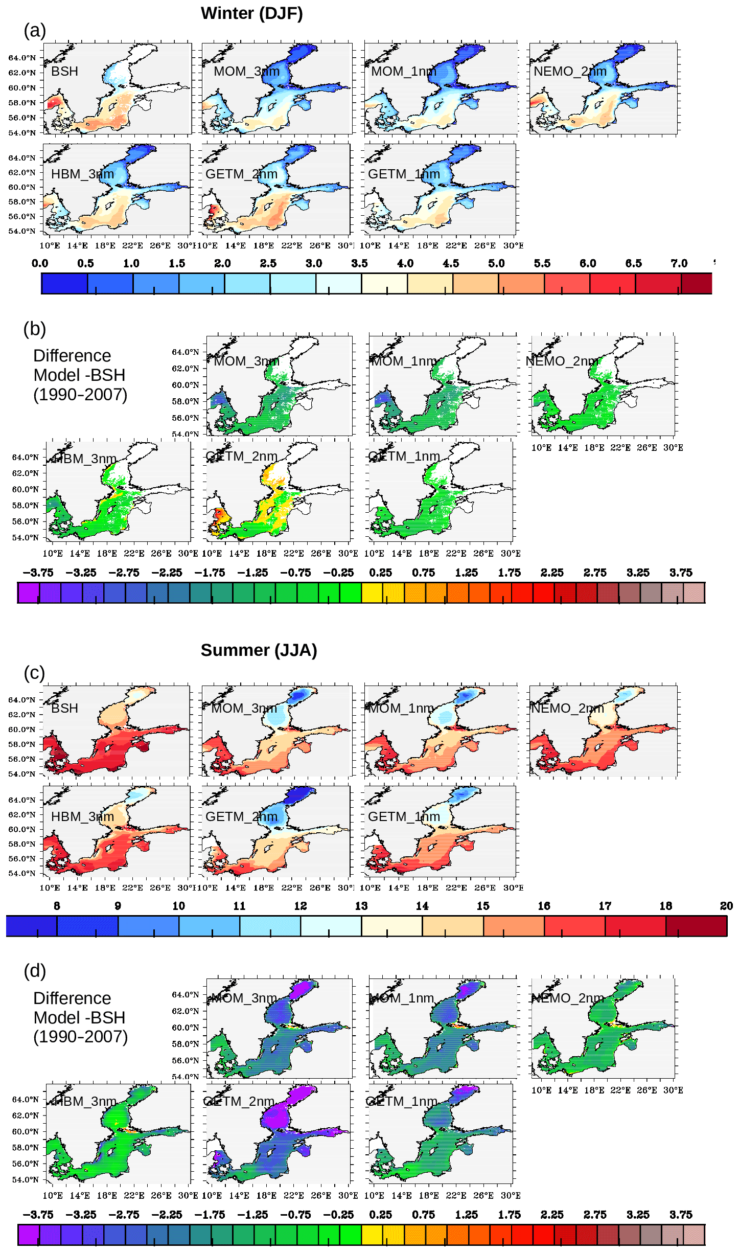
Figure 3(a) Comparison of modeled winter SST with a satellite product from the Federal Maritime and Hydrographic Agency of Germany (BSH). (b) Difference between the models and the satellite product for winter. Panels (c) and (d) are as for panels (a) and (b) but for summer climatology. Note that winter SST coverage from the satellite product is incomplete.
A number of modeling groups have recently started to produce BMIP model runs. Here we provide a first assessment of temperature and salinity. As the analyzed simulations differed with respect to the model initialization, results before 1970 were not interpreted. The effect of different spinups after 1970 on suprahalocline waters in the Baltic Sea was assumed to have been minor. For the HBM, a different runoff forcing was used. However, even with these minor deviations, the model outputs analyzed below constitute a highly harmonized data set, which is unlike those obtained in previous model comparisons.
3.1 Assessment of mean climatologies
In the following, water temperature and salinity are briefly assessed in the models. Our aim was not to provide a comprehensive validation but to demonstrate the marked differences between models despite the same forcing. For climate applications, differences in the spatial characteristics of the models should be considered (Placke et al., 2018; Gröger et al., 2019). However, despite the long history of national and international Baltic Sea research, no long-term mean climatology product for water salinity and temperature is available that satisfyingly serves the needs of climate research (Kent et al., 2019; Zumwald et al., 2020; Hegerl et al., 2021). Therefore, for comparison, we use gridded data sets of remote sensing SST data, obtained from the BSH, for the period 1990–2007. In addition, a Baltic Sea reanalysis data set covering 1970–1999 (Liu et al., 2017) is provided in Sect. S3. Both data sets are characterized by uncertainties and shortcomings, mainly arising from limited observations in space and time. Consequently, limited observational constraints were available for the data assimilation product (Liu et al., 2017). Also, no in situ data from the Baltic Sea were used in the calibration of the remotely sensed data from the BSH. The mean seasonal cycle was analyzed based on in situ data derived from the SHARK database hosted by the Swedish Meteorological and Hydrological Institute (https://sharkweb.smhi.se/hamta-data, last access: 16 November 2022).
In all models, winter SSTs (Fig. 3a) were lowest in the Bothnian Sea, Bothnian Bay, the Gulf of Finland, and the Gulf of Riga. In the shallower Gulf of Finland and Gulf of Riga, where the heat inventory was rather low, the SSTs adapted rapidly to the cold winter atmosphere. In the open Baltic proper, the sea ice in the Bornholm and Arkona basins was mostly absent, such that the stronger winter winds together with convective mixing supported exchange with warmer waters from deeper layers. The satellite-based observations (Fig. 3a) revealed strong horizontal SST gradients between the cold, shallow Kattegat/Sound/Great Belt, where the heat inventory was low, and heat loss was rapid, and the deeper Skagerrak in the northeast, where vigorous cyclonic circulation and the subsequent Ekman-induced upward transport of warmer, deepwater together with wind-induced deep mixing led to higher SSTs. In the models that included parts of the Skagerrak (HBM_3nm, MOM_3nm, MOM_1nm, and NEMO_2nm), these gradients were also present but were generally less well pronounced than according to the satellite product. With the exception of GETM_2nm, all models systematically simulated winter SSTs that were lower than those in the BSH satellite data (Fig. 3b). This was also the case in comparisons between the models and the reanalysis data set (Sect. S3). With the exception of GETM_1nm and NEMO_2nm, the model–BSH biases (Fig. 3b) were largest near the lateral boundaries, thus demonstrating the importance of boundary conditions in the realizations of individual models. The high SSTs in GETM_2nm along the Danish east coast (Fig. 3a) caused strong positive biases in comparison with the BSH climatology (Fig. 3b) and the reanalysis data (Sect. S3).
During summer, meteorological forcing was characterized by calm winds and stronger solar radiation, which promoted an intense thermal layering of the uppermost water column. In the open sea, air–sea coupling was affected by the presence of a strong thermocline that reduced exchange with cooler waters from greater depths. The subsequent reduction in the effective water column heat capacity made the SSTs more prone to variations in meteorological forcing than was the case in winter.
Hence, the seasonal and spatial characteristics of the thermocline, and its intensity and its position in the water column, are a key parameter for the evolution of SSTs, right from their formation in spring to their disappearance in autumn, and are well investigated in the Baltic Sea (e.g., Eilola, 1997; Liblik and Lips, 2011, 2019; Hordoir and Meier, 2012; Chubarenko et al., 2017; Gröger et al., 2019).
Similar to winter, the summer SSTs determined in the simulations were lower than those of the satellite product (Fig. 3c, d). The cold biases were considerably higher in summer than in winter and, in some models, exceeded −2 K. However, the satellite product may reflect the water skin temperature (rather than the vertical mean temperature across the respective first model layer), which was not explicitly represented in the models. Generally, the biases between the models, the satellite data, and the reanalysis data were much more pronounced in summer than in winter.

Figure 4(a) Correlation of interannual winter sea surface temperature variation between models and the satellite product. (b) Correlation of interannual winter sea surface temperature variation between models and the satellite product.
An important prerequisite for the use of the models in climate applications is their ability to correctly represent the interannual variability and to respond to long-term variations in atmospheric forcing (e.g., Gröger et al., 2015, 2019). Figure 4a shows an overall high interannual correlation for the winter season, with values mostly around 0.7 or higher. Hence, despite the sometimes large discrepancies in the mean climatologies (as shown in Fig. 3), the interannual variations in models fit those in the satellite data. However, in the Bothnian Sea and Bothnian Bay in summer (Fig. 4b), the correlation values were low and in some cases <0.3. For the northernmost parts of the Bothnian Bay, remnant sea ice floes from the previous winter can affect vertical mixing and affect SSTs. Thus, in these regions, realistic sea ice cover is essential.
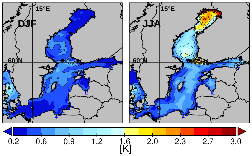
Figure 5Intermodel standard deviation of SST for winter (December–February, DJF) and summer (June–August, JJA). The standard deviation was calculated from the six models (MOM_3nm, MOM_1nm, GETM_2nm, GETM_1nm, HBM_3nm, and NEMO_2nm).
The intermodel spread, as summarized by the intermodel standard deviations (Fig. 5), is clearly higher in summer compared to winter. However, the summer pattern also shows a significant reduction in the spread near the coasts. In these shallow environments, no stable thermal stratification develops, such that these small waterbodies rapidly adapted to identical atmospheric forcing. Notably, the models' representations of coastal upwelling along the Swedish east coast did not increase the spread, in contrast to open-sea areas, where the spread was systematically higher than in coastal regions. This highlights the importance of the internal model dynamics that control the depth and intensity of the thermocline. The lower intermodel spread during winter was likely related to stronger wind-induced and convective mixing, which promote a strong heat flux from the ocean. In areas with stable sea ice conditions, i.e., the Bothnian Bay, the eastern Gulf of Finland, and the Gulf of Riga, the very low wintertime spread in all models could be explained by a SST roughly equal to the freezing point temperature.
The large SST spread in the Bothnian Bay in summer may have been due to the different melting rates in the models, since sea ice break up is highest in May/June and is followed by a warming of the surface water layer (Fig. 5).
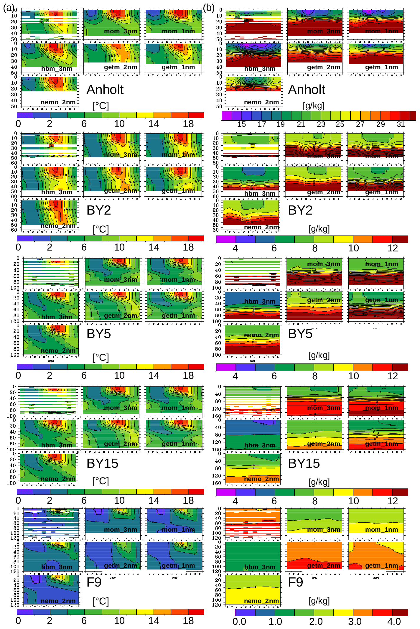
Figure 6Multiyear (1990–2009) mean seasonal cycle of water column temperature (a) and salinity (b) at selected monitoring sites in the Baltic Sea. See the text for further explanation. The upper-left plot of each panel displays the seasonal cycle based on the SHARK data set. Note the different color scales for salinity at the Anholt and F9 stations.
3.2 Mean seasonal cycle
The seasonal cycle of water temperature and salinity was assessed at selected stations (Fig. 6) located at key sites along a transect that roughly followed the pathway of imported saltwater. Hence, conditions at the stations ranged from shallow waters upstream of the overflow region (Anholt; Fig. 1b) and open-sea conditions in the southern Baltic (Arkona Basin BY2 and Bornholm Basin BY5) to deepwater conditions in the Baltic proper (east Gotland Basin BY15) and, finally, to the Bothnian Bay (F9), where there is no notable halocline but seasonal ice cover has a significant effect.
3.2.1 Water temperature
Station Anholt
The strongest seasonal cycle along the transect was determined at Anholt station (Fig. 6), which is representative of the shallow water conditions in the southern Kattegat (Fig. 1b). The amplitude of the seasonal temperature cycle was most pronounced in the HBM_3nm and the two MOM models and was slightly overestimated compared to the SHARK data set. In particular, the surface-to-bottom temperature gradients during summer were stronger in the two MOM simulations than in the simulations of the other models. NEMO reaches only a water depth of ∼25 m, and so water temperatures do not drop below 14 ∘C during summer.
Stations BY2 and BY5 (Fig. 6) are located in the Arkona Basin and Bornholm Basin, respectively, and thus further downstream of the overflow region. The thermal structure at BY2 and BY5 (Fig. 6a) reflects the well-studied cold intermediate layer (CIL; Chubarenko and Stepanova, 2018; Liblik and Lips, 2019; Dutheil et al., 2021), the remnant of a water mass that formed during the previous winter at a depth between 20 and 60 m and became encapsulated during the subsequent warm season, along with the development of a strong thermocline. The CIL is more pronounced at BY5, a deeper station that represents more open-ocean conditions. When the storm season starts in autumn, the warmer surface waters are mixed further downward. Consequently, the surface rapidly cools, while, after a short delay, the intermediate water warms, finally terminating the lifetime of the CIL (Fig. 6a). This was well reproduced by all of the studied models.
Station BY15 represents fully open-sea conditions in the eastern Gotland Basin (Fig. 1b). In agreement with the observations, in all models, the thermocline at this station was shallower than at all other considered stations (Fig. 6a). At the deep layers, seasonal variation is low and ranges in all models between ∼0.0 and ∼0.5 ∘C.
A comparison with the in situ data for BY15 obtained from the Baltic Environmental Database (BED) of the Baltic Nest Institute (BNU; Sect. S4) showed a reasonable representation of the seasonal SST cycle in open-ocean environments. The monthly mean climatologies calculated by the models were well with within the standard deviations calculated for each month from the BED. Besides this, in the GETM_2nm, the summer is colder, and the winter is warmer, such that the seasonal cycle was less prominent than according to the BED data. In the two MOM versions, winter months are systematically colder, but there was good agreement with summer data from the BED. However, the GETM_1nm best reproduced the BED cycles.
Station F9 is the northernmost site and located in the Bothnian Sea. At this station, water temperatures below 0 ∘C were recorded, in the SHARK data and in the two MOM versions, up to March/April. During summer, the weakest thermocline (i.e., lowest temperature gradients) was again that of the GETM_2nm.
3.2.2 Salinity
Station Anholt
In line with the abovementioned strong thermal seasonal cycle, we also found a strong seasonal cycle in surface salinity (Fig. 6b). The surface-to-bottom salinity gradients are highest at this stations. Among the models, the two MOM versions have the highest gradients, which suggests that vertical mixing was underestimated in the MOM compared to the other models. In the NEMO_2nm, the water depth at this site was clearly shallower than in the other models, such that salinities >32 g kg−1 were rarely reached.
Stations BY2 and BY5
The two sites receive freshwater inputs from rivers, while saltwater is supplied by the North Sea. This results in strong vertical salinity gradients, which were most pronounced in MOM and GETM_1nm and weakest in HBM_3nm, NEMO_2nm, and GETM_2nm (Fig. 6b). In particular, HBM_3nm underestimated salinity over the whole water column, which suggested that a potential bias in vertical mixing was not the only explanation; rather, the intensities of saltwater inflows from the North Sea were likely underestimated. Furthermore, in the HBM_3nm, the recommended BMIP river runoff forcing was not applied. Runoff differences between data sets will add to the uncertainty in near-coastal salinity.
Station BY15
With further distance from the North Sea, the deepwater salinity becomes markedly lower than at stations BY5 and BY2. Our use of a common forcing data set provides the first assessment of how large BMIP models can differ due to their internal dynamics, such as vertical mixing or inflows. Apart from HBM_3nm, which was not designed to focus on MBIs, the GETM_2nm and NEMO_2nm are the models with lowest salinity in the deep layer but highest salinity in the upper layers of all models, suggesting stronger vertical mixing. Stronger mixing was also reflected by the rather low vertical salinity gradients.
Station F9
At station F9 located in the Bothnian Sea, salinities according to the SHARK data are in the range between ∼3 and 4 g kg−1. This range was best reproduced by the two GETM versions, while lower salinities were obtained in the other models (NEMO_2nm, MOM_1nm, MOM_3nm, and HBM_3nm).

Figure 7Intermodel comparison of a long-term time series of (a) the mean summer (JJA) and (b) winter (DJF) SST in addition to the annual mean (c) bottom temperature and (d) salinity at selected sites in the Baltic Sea. Numbers in the respective panels denote intermodel standard deviations averaged over the entire period 1961–2018.
3.3 Long-term variability in temperature and salinity
Long-term variability was briefly assessed by the modeled time series of temperature and salinity at the same stations used to examine the mean climatological cycles (Fig. 6). Generally, the models differed more when the interannual variability was large, exemplified by the winter SSTs at Anholt station and the summer SSTs at station F9 (Fig. 7). At stations BY2, BY5, and BY15, representing open-sea conditions with successively larger water depths, good agreement between the models was obtained for both winter and summer SSTs. The intermodel standard deviation for SST increased from the shallower site BY2 toward deeper sites BY5 and BY15, indicative of greater meteorological control at shallower than at deeper sites. In agreement with the analysis of the mean climatology (Fig. 5), the long-term-averaged intermodel standard deviation of the SSTs was systematically higher during summer than in winter (Fig. 7a).
Interannual SSTs co-varied quite well across the models, at all sites, and for both seasons (Fig. 7a, b). For the stations Anholt, BY15, and F9, summer SSTs were systematically lower in GETM_2nm than in the other models. Covariation was generally worse for bottom than for surface temperatures (Fig. 7c). This was most obvious at the deep stations of BY15 and F9, which are less well constrained by meteorological forcing. The spread in bottom temperatures at BY15 was extraordinarily low after the MBIs that took place in 1993. The strength of the latter event was well reflected in all models by a corresponding shift to higher bottom salinities, although the corresponding intermodel spread in salinities was quite large.
All in all, model agreement in bottom temperature and salinity was lowest at the deepest stations (BY5 and BY15), as indicated by the long-term-averaged intermodel standard deviations. Note that nearly no interannual variability in bottom salinity at Anholt was recognized by MOM_3nm, and the mean salinity was higher than in all other models (Fig. 7d). This suggested a more or less stable inflow of saltwater from the North Sea into the Kattegat.
The dynamics of MBIs, as reflected in the deep salinity at BY15, accounted for an intermodel spread that was by far the largest (Fig. 7d). While, in the simulations, at least those for the decades after 1990, individual inflows were consistently recorded (although with varying amplitude), the first ∼30 years may have been influenced by long-term model drifts. This was especially the case for models in which the mean equilibrium state strongly differed from the initialization state, as occurred in the HBM_3nm. Comparison with the high-resolution in situ data from the BED showed that the results of the two MOM versions and GETM_1nm were closest to the observations (Sect. S5). However, the two MOM versions apparently underestimated low-amplitude variations, as indicated by the relatively smooth curves, particularly during the early decades.
Station F9 is located farthest from the overflow region, and its interannual variability is accordingly low. A notable drift over the entire period was determined in the HBM_3nm and may have been related to differences in runoff forcing or to physically and numerically induced mixing that was too large in that run (Burchard and Rennau, 2008). All models, but the operational setup HBM_3nm, show no significant drift in the deep salinities at stations F9 and BY15 and so confirm the length of the spinup run of 44 years.
3.4 Brief assessment of model spread of extreme temperatures
The oceanic and atmospheric models applied in climate sciences are typically developed to reasonably reproduce long-term temperature climatologies averaged over several decades, whereas extreme temperatures are less often considered. However, the BMIP will also investigate the impact of climatic extremes and short-term events, such as heat waves (e.g., Suursaar, 2020). The intermodel standard deviation for the 5th, 25th, 50th, 75th, 85th, 95th, and 99th percentiles of the temperature averaged over the whole Baltic Sea are presented in Fig. 8a, which clearly shows that the standard deviation, and thus model uncertainty, increases at high temperature regimes. Again, this conclusion could be drawn because atmospheric forcing was the same in all models, thus further demonstrating the added value of the BMIP.
Model spread with respect to water depth is shown in Fig. 8b. A more-or-less linear increase with depth can be seen that is largest in the bottom layer. This was expected, as deepwater properties are less constrained by atmospheric forcing such that initialization, model numerics, and the parameterization of subgrid processes become more important.

Figure 8(a) Intermodel standard deviation calculated from the 5th, 25th, 50th, 75th, 85th, 95th, and 99th percentile surface temperatures. The percentiles represent area averages over the whole Baltic Sea. (b) Intermodel standard deviation of depth-interval-averaged water temperature. Standard deviations are calculated from spatial averages over the whole Baltic Sea from each of the six models. The analysis covered the period of 1990–2007.
4.1 Marine heat waves
Climate warming increases the risk of extreme events in ocean climate. For example, MHWs in the world ocean are expected to be more frequent and intense in a warmer climate (Oliver et al., 2019). Due to its low water volume and limited exchange with the open ocean, the Baltic Sea is especially sensitive to external changes in the heat supply. Unlike the North Sea, which fully mixes during winter and is well ventilated by waters from the North Atlantic within a few years, in the Baltic Sea the perennial halocline limits heat exchange between the surface and deeper layers. Accordingly, larger and smaller warming of the surface and subhalocline layers, respectively, can be expected. In the Baltic Sea models analyzed herein, this has been well reflected by the larger increase in surface than in bottom temperatures since the mid-1980s (Fig. 9). Moreover, extreme SSTs can increase more than mean SSTs. As shown in Table 2, higher warming trends for the annual maximum temperature than for the annual mean temperature were determined by all of the models. Likewise, the higher cross-model standard deviation in the maximum temperature trends than in the mean temperature (Table 2) implied higher uncertainties in the high temperature regime. These results highlight the need for studies on the processes leading to extreme SSTs in the Baltic Sea.
Table 2Comparison of yearly mean and maximum temperature trends averaged over the whole Baltic Sea. Note that SD is for standard deviation.
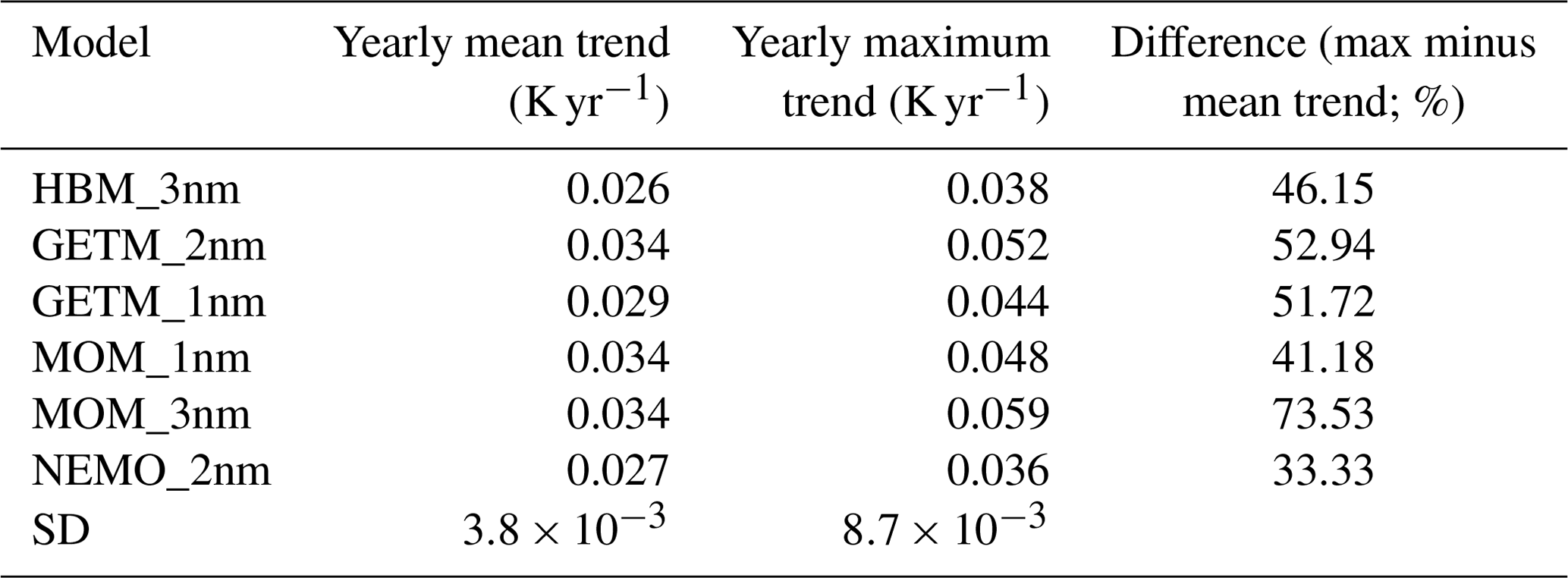
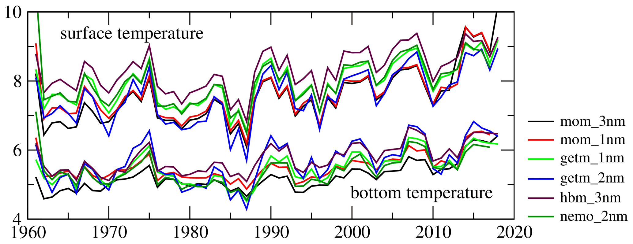
Figure 9Annual mean surface and bottom water temperatures averaged over the entire Baltic Sea.
Figure 10 shows the yearly mean area affected by different classes of MHWs. The models were compared with the reanalysis data set covering the reference period of 1970–1999 (Liu et al., 2017), which was characterized by two distinct maxima, in 1975 and 1990, when areas of >125 000 km2 were affected vs. 000 km2 during the intervening period. These two peaks were well reproduced by the models. The longer record of the BMIP models allowed the identification of pronounced periods of high MHW extensions, with peaks occurring in 1975, 1990, 2002, 2009, 2016, and 2018, thus pointing to roughly decadal variations until 2002 and the potential increases due to climate warming afterwards. The weak imprint of MHWs in the second half of the 1970s and 1980s might be related to the extraordinarily low North Atlantic SSTs recorded during those years (Kushnir, 1994). In all of the models there was a trend toward more extended MHWs after ∼1990, consistent with the climate warming trend during that same time (e.g., Dieterich et al., 2019; Gröger et al., 2019; Meier et al., 2022; Placke et al., 2021; Dutheil et al., 2021). Before ∼2000, MHWs were rarely above the moderate class, whereas strong MHWs (class II) became more prominent thereafter. The intermodel differences were rather low, most obviously during the early period, but the MOM simulations yielded very highly extended MHWs, especially during the past decade.
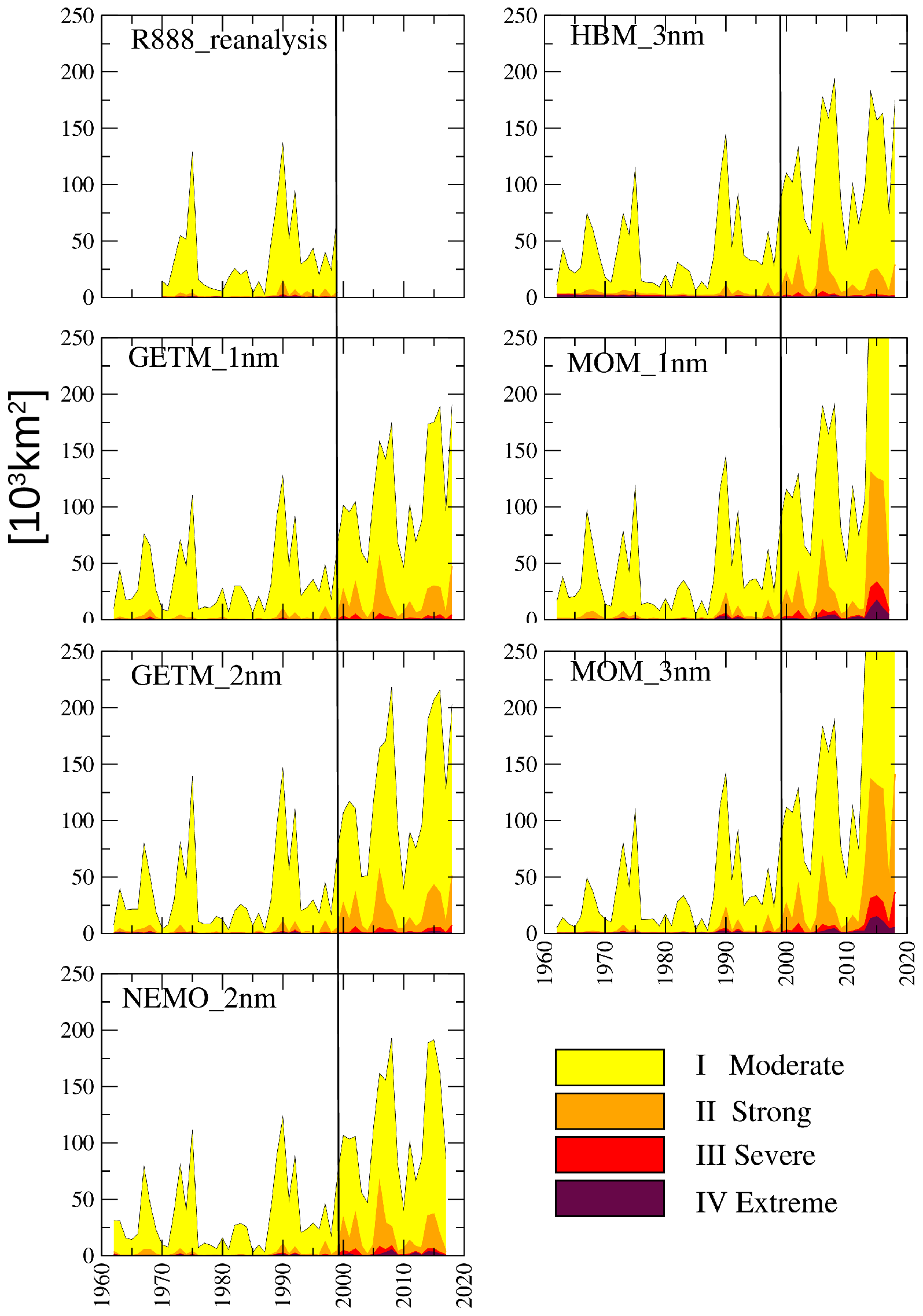
Figure 10Yearly average spatial sea surface extent of MHWs over the entire Baltic Sea. The reanalysis data set refers to Liu et al. (2017). The vertical lines indicate the end of the reanalysis period in each panel. Classification was done after Hobday et al. (2018).
Next, MHW frequency was analyzed by counting the number of periods with at least 5 consecutive MHW days (class I or higher). MHWs separated by only 1 or 2 d were counted as one MHW. Determinations were done separately for the 25-year periods of 1965–1989 (early period) and 1994–2018 (late period). The results are shown in Fig. 11. For the early period (Fig. 11a), all models indicated that MHWs were most frequent in the Kattegat, the Arkona Basin, and in Bothnian Bay, i.e., shallow areas or areas with seasonal sea ice cover. The largest intermodel differences, as indicated by the ensemble standard deviation (Fig. 11a; rightmost panel), occurred in the Bothnian Bay and in the easternmost Gulf of Finland and were likely related to differences in the modeled sea ice cover which affected the ocean–atmosphere heat exchange.

Figure 11(a) Total number of MHWs with a duration of at least 5 consecutive days (class I or stronger) during the period 1965–1989. (b) Average MHW duration (class I or stronger). (c) Relative change in the number of MHWs between the period 1994–2018 and the period 1965–1989. (d) Same as panel (c) but for the average MHW duration. Note the different scaling of panels (c) and (d). STDDEV in the rightmost column indicates the cross-model standard deviation and has its own color bar.
The average MHW duration varied spatially between 8 and 25 d, as shown in Fig. 11b. Longest MHWs occurred in the Bothnian Bay. The ensemble spread was highest in the Bothnian Bay and locally elevated in the Bothnian Sea and the central Baltic proper, as indicated by the ensemble standard deviation. In shallow regions and along the coasts, MHW duration was consistently short, as these areas are more prone to variable meteorological forcings that may disrupt MHWs, such as storm events or cold water intrusions from the open sea. As MHWs of longer duration will ultimately limit the number of possible MHWs within a given time period, the models showed a negative relationship between average MHW length (Fig. 11b) and MHW frequency (Fig. 11a). However, the correlation between the duration and number of MHWs differed considerably between models, with for MOM_3nm, for MOM_1nm, 7 for GETM_2nm, 5 for NEMO_2nm, for GETM_1nm, and for HBM_3nm (averaged in each case over the Baltic Sea).
In the late period of 1994–2018, MHWs were almost uniformly more frequent and of longer duration (Fig. 11c, d). Common to all models is the strong increase in the Gotland Basin, where relative increases exceeded 200 %. Both MOM versions showed an extraordinary increase in average MHW duration, thus offering an explanation for the extraordinarily large spatial extension of MHWs that occurred during the last decade (Fig. 10), as a longer duration favors a larger spatial extension, and vice versa. In the HBM_3nm and GETM_1nm, the changes in the frequency and duration were smaller than in the other models.
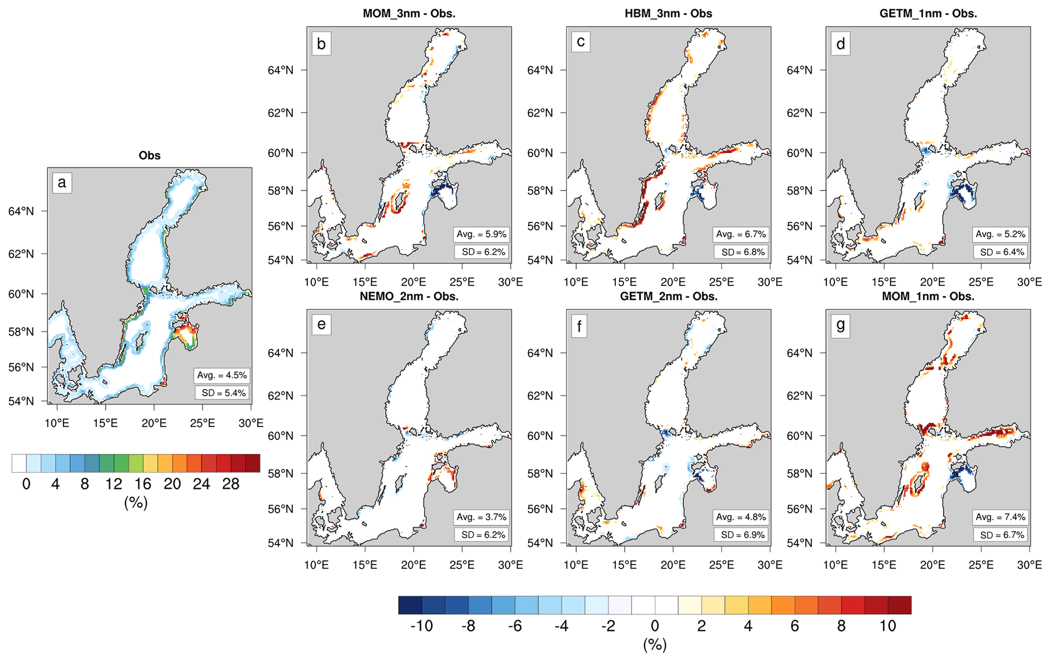
Figure 12Annual upwelling frequencies (in %). In panel (a), the observations are shown. In panels (b)–(e), the errors made by models (b) MOM_3nm, (c) HBM_3nm, (d) GETM_1nm and (e) NEMO_2nm, (f) GETM_2nm, and (g) MOM_1nm are shown. The average and standard deviation are shown in the bottom-right corners.
4.2 Coastal upwelling
Figure 12 displays the annual upwelling frequencies according to the BSH satellite data and the deviation therefrom in each simulation. In the former, the average annual upwelling frequency over the Baltic Sea was 4.5 %. Upwelling areas were concentrated along the Swedish coast and in the Gulf of Riga, where upwelling frequencies can exceed 20 %. In other coastal regions, the annual upwelling frequency was <10, resulting in a spatial standard deviation of 5.4 %. Along the zonal coasts, we are not able to disentangle whether the bias is due to the model or due to the limitation of the upwelling detection method.
All hindcast simulations, except that of NEMO_2nm, overestimated the annual upwelling frequencies compared to the observations but with some discrepancies. Thus, according to HBM_3nm, MOM_3nm, and GETM_1nm, the annual upwelling frequency was 6.7 %, 5.9 %, and 5.2 %, respectively. In the NEMO_2nm simulations, the annual upwelling frequency was 3.7 % and thus underestimated. Overall, the spatial pattern of the annual upwelling frequencies was well represented in all hindcasts, with a similar bias pattern between the models except NEMO. Hence, GETM_1nm, MOM, and HBM_3nm tended to underestimate the upwelling frequencies in the Gulf of Riga and overestimate them along the Swedish coast, around Gotland, and in the Gulf of Finland (Fig. 12). The opposite spatial bias pattern was determined for NEMO_2nm, which shows, likewise, a very small bias overall. From the above descriptive statistics alone, it is difficult to speculate about the different bias pattern seen in NEMO_2nm, in particular in the Gulf of Riga. However, possible reasons could include the model formulations for influencing variability, such as atmosphere-to-ocean momentum transfer or the seabed–water boundary layer. Thus, overall, the spatial standard deviation was overestimated by 6.2 % (MOM_3nm and NEMO_2nm) to 6.8 % (HBM_3nm) compared to 5.4 % in the observations. The high-resolution versions of MOM_1nm and GETM_1nm (Fig. 12d and g) show, in most regions, a larger bias to the observations than their coarse-resolution versions MOM_3nm and GETM_2nm (Fig. 12b, f).
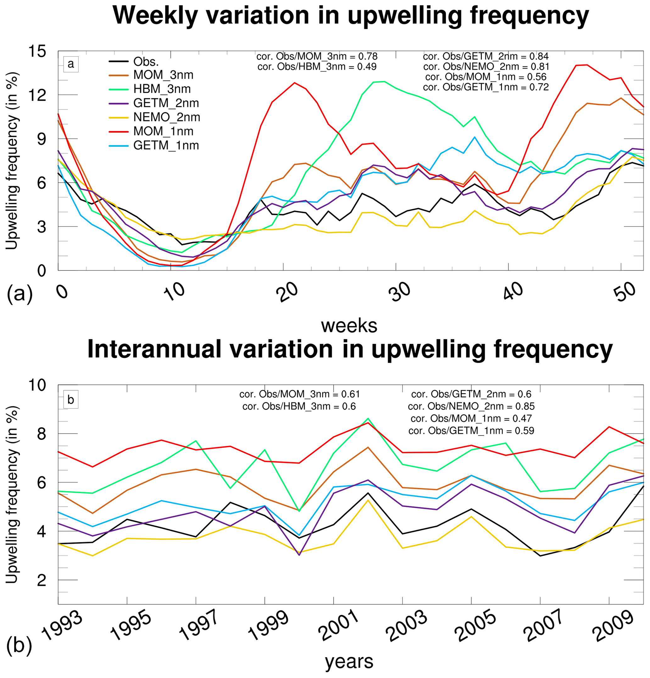
Figure 13Weekly (a) and interannual (b) variations in upwelling frequencies (in %) according to observations (black lines) and the models MOM_1nm, MOM_3nm, HBM_3nm, GETM_1nm, GETM_2nm, and NEMO_2nm (red, green, blue, and yellow lines, respectively). The correlations between observations and models are shown in the top-right corners.
Figure 13 shows the weekly and interannual variations in the observed and modeled upwelling frequencies. According to the observations, the weekly upwelling frequency averaged over the Baltic Sea varied from 2 % to 7 %, with minimum values occurring at the end of winter and in early spring, i.e., between weeks 5 and 15, and maximum values at the end of the year, around week 50. From spring to autumn, the upwelling frequency was also high (reaching 6 %). From 1993 to 2010, the annual upwelling frequency was characterized by a strong interannual variability, varying by a factor of 2 (from 3 % to 6 %), with a frequency between 3 and 6 years (determined by wavelet analysis).
The mean weekly variations in upwelling frequency were well modeled, with the correlations between observations and the models ranging from 0.49 (HBM_3nm) to 0.81 (NEMO_2nm), although the models tended to overestimate the amplitudes. The GETM_2nm, MOM_3nm, and HBM_3nm models underestimated the upwelling frequencies between weeks 5 and 15 and overestimated them from week 20 to the end of the year. These biases were reduced in NEMO_2nm, in which the weekly variation was similar to that in the observations. The mean weekly amplitude was thus 11 % in MOM and HBM_3nm, 9 % in GETM_2nm, and 5.6 % in NEMO_2nm, compared to 5.6 % in the observations. The interannual variability was also well modeled, with correlations between observations and the models of ∼0.6 for GETM_2nm, MOM_3nm, and HBM_3nm and 0.85 for NEMO_2nm. The overestimation or underestimation of annual upwelling frequencies shown in Fig. 13 were consistent with the results presented in Fig. 12. In contrast to the biases in the mean weekly upwelling frequencies, those in the interannual upwelling frequencies were almost stationary.
To conclude, the biases in the hindcast simulations of GETM_2nm, MOM_3nm, and HBM_3nm were similar and characterized by an overestimation of the annual mean upwelling frequency and of the spatial variability, while opposite and smaller biases were obtained with the NEMO_2nm simulation. The upwelling frequency was overestimated around Gotland, along the southern Swedish coast, and in the Gulf of Finland and underestimated in the Gulf of Riga. The weekly amplitude of the upwelling frequency was also overestimated, but the interannual variability was well simulated. Overall, opposite conclusions were derived from the NEMO_2nm simulation.
The upwelling analysis highlighted the differences in the BMIP models and thus the importance of systematic intermodel comparisons. Deeper analyses, for instance, intermodel comparisons aimed at determining the contributions of the individual mechanisms responsible for upwelling events (e.g., Ekman pumping and hydrodynamic circulation), could provide insights into the reasons for the differences in upwelling (e.g., parameterization of internal waves or air–sea fluxes).
4.3 Water column stratification
The Baltic Sea is stratified by both a permanent halocline and a seasonal thermocline. The depth and strength of these clines vary spatially and over time, with the summer thermocline developing in late spring and lasting until the transition summer/autumn. A good model representation of thermocline development is therefore especially important for biogeochemical models, as it must accurately depict the timing and intensity of the spring bloom.
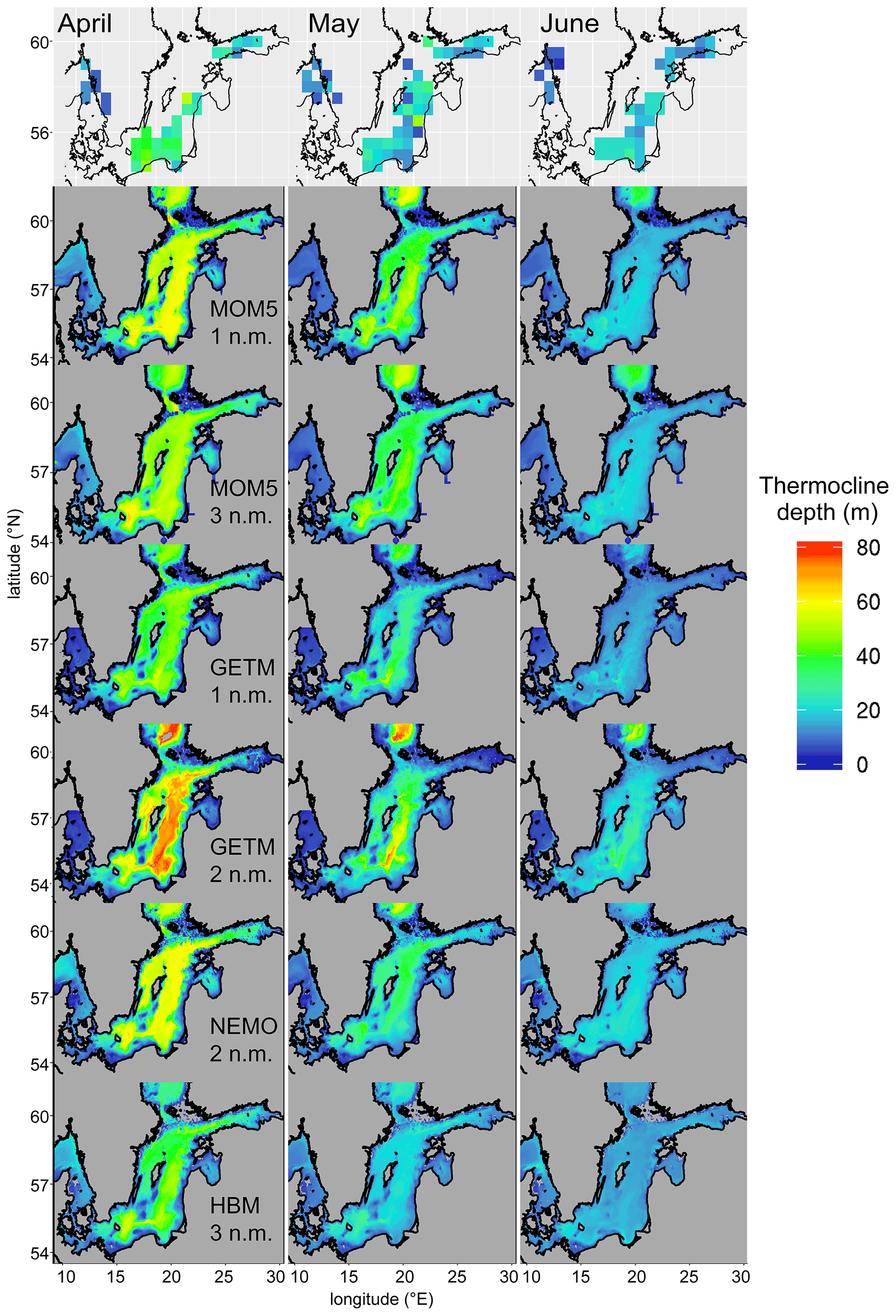
Figure 14Thermocline depth as derived from ICES observational data (uppermost row) and from different BMIP models. Gray areas in the ICES maps indicate a lack of data, in the BMIP model maps they denote values above 60 m. Note, the maps are cut off in the north due to lack of sufficient ICES data for the cline calculation.
As an example, the typical climatological development of the summer thermocline, as determined in the BMIP models, is shown in Fig. 14. For comparison, the depths included in the figure are the same as those calculated from the observed vertical profiles using the ICES database. Point observations were grouped with vertical profiles based on a common latitude, longitude, and date. Vertical profiles less than 60 m deep and that included jumps in the vertical coordinate >5 m were excluded from the analysis. For the period 1960–2018, the cline depths for each of the observed profiles were calculated. Finally, a monthly climatology was created by taking the median of all values in a calendar month for every box of a horizontal grid. The median rather than the mean was used to reduce the sensitivity to outliers. Finally, at least five values per box were required to consider the median as valid.
The results showed that, in April, all of the considered models overestimated the thermocline depth, which, in the southern part of the central Baltic Sea, was ∼30 m. The overestimation was lowest in the coarser models (HBM_3nm and the MOM_3nm) and in NEMO_ 2nm. Near-coastal regions, where low values of the thermocline depth were determined by the models, were excluded from the observational climatology because of the required minimum depth of 60 m. The observations showed that the summer thermocline formed already in May, with the thermocline depth dropping to ∼20 m. This was reasonably captured by the HBM_3nm and NEMO_2m models, whereas, in the GETM_1nm and especially the two MOM models, thermocline shallowing was delayed. In June, the models determined a reduction in the thermocline depth to ∼20 m, which was a slight underestimation compared to the observed value. The GETM_1nm model differed from the others, as it showed a clearly enhanced thermocline depth in the deeper parts of the southern Baltic proper.
Further detailed analyses of model output may reveal the reasons underlying the difference in the timing of thermocline formation despite identical atmospheric forcing, which may involve the model formulations for turbulence and the effect of grid resolution or bottom friction (e.g., Krauss, 1981; Eilola, 1997; Liblik and Lips, 2011, 2019; Hordoir and Meier, 2012; Chubarenko et al., 2017; Gröger et al., 2019).
In addition to the intermodel comparisons presented herein, a very high-resolution model for the central Baltic Sea is under development within the framework of the BMIP collaboration. The aim of this computationally challenging project is to investigate large-scale ocean circulation with respect to the role of mesoscale and submesoscale processes. Scientific questions regarding the importance of eddies and other small-scale processes in the exchange of dissolved nutrients and toxins between the coastal zone and the open sea will be examined as well.
The model setup is built on the GETM source code, and the model domain covers most of the Baltic Sea, including the Kattegat and Danish straits and both the Gulf of Finland and the Gulf of Riga. The northernmost part of the Baltic Sea, i.e., the Gulf of Bothnia, consisting of the Bothnian Sea and Bothnian Bay, has been replaced by an open boundary.
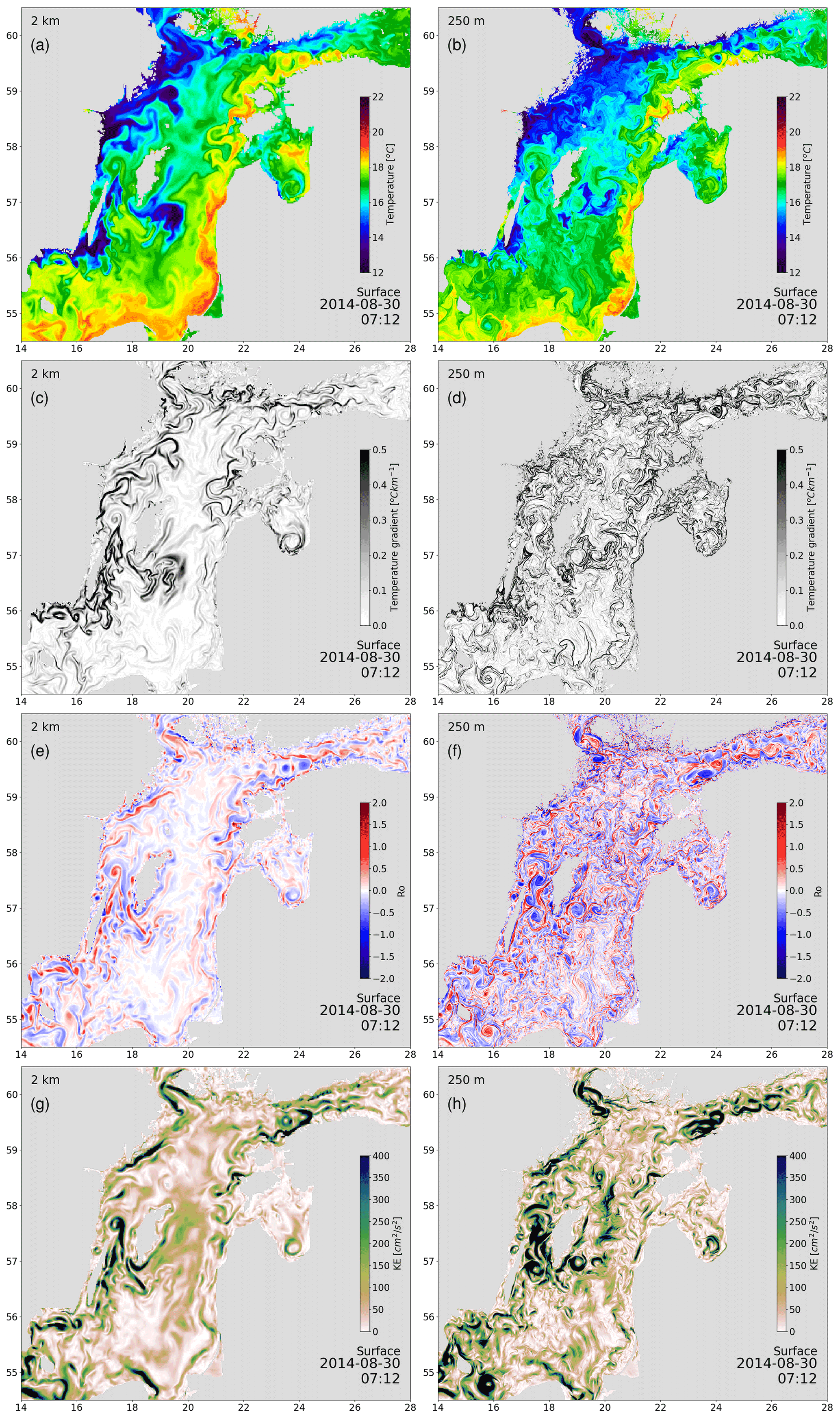
Figure 15(a, b) Snapshot of surface layer temperature (∘C). (c, d) Temperature gradient (∘C km−1). (e, f) Rossby number and (g, h) kinetic energy (cm−2 s−2), as obtained from the low-resolution (1 n.m., left) and high-resolution (250 m, right) simulation for the Baltic Sea.
The importance of high-resolution simulations is illustrated in Fig. 15, in which different parameters simulated with low (1 n.m.) and high (250 m) resolution are compared. In general, large-scale patterns were well simulated by both. In each case, there was a strong south-to-north gradient in the simulated surface temperature fields, with the highest (lowest) temperatures in the southern (northern) part of the Baltic Sea. In addition, in the northwestern Baltic proper, a large patch of cold water of upwelling origin along the Swedish coast and advected from the Gulf of Bothnia was well visible in both simulations. In contrast to the situation in the north, warm water in the coastal regions of the southern and eastern Baltic proper were determined in the two simulations. The largest differences between the results obtained at high vs. low resolution involved several details of the simulations. First, the low-resolution model was generally unable to produce strong lateral gradients in open-sea areas, except in cases in which strong fronts already occurred due to mesoscale activity (upwelling along the Swedish coast). Second, eddy activity in the open sea was much smaller in the 1 n.m. simulations than in the 250 m resolution simulations, with much weaker (geostrophically balanced) eddies in the low-resolution run, whereas in the high-resolution run much stronger and ageostrophic eddies (Rossby number >1) were produced, both in the coastal area and in the open sea. Weaker eddy activity in open-sea areas with low resolution were also visible in the spatial maps of kinetic energy.
The overall purpose of the high-resolution simulations was to analyze the role of eddies in the Baltic Sea (e.g., Lips et al., 2016; Väli et al., 2017, 2018). Several studies of the mean circulation (e.g., Lehmann et al., 2002; Meier, 2007; Placke et al., 2018) and of long-term nutrient transport (e.g., Eilola et al., 2012) performed using low-resolution models are available, and they provide evidence of large-scale gyre structures with strong persistent currents in the eastern Gotland Basin and of an overall estuarine circulation in the Baltic Sea. However, these models were largely eddy-permitting rather than eddy resolving. Vortmeyer-Kley et al. (2019a, b) attempted to quantify the number of eddies and their lifetime using higher-resolution models, while Zhurbas et al. (2019a) provided a qualitative comparison of observed and simulated eddies. The importance of eddies in transport within the Baltic Sea is therefore still unclear. Long-term, high-resolution simulations that allow the representation of submesoscale structures are likely to yield important information.
The BMIP provides almost 60 years of physically consistent data on meteorological and hydrological forcing, for use in Baltic Sea ocean modeling. This study, the first systematic model intercomparison, revealed marked local-to-regional model differences in simulated temperature and salinity, in vertical thermal and haline stratification, and in distinct climate and environmental indices (e.g., heat waves, upwelling, and stratification). Our results thus emphasize the role of internal model dynamics, in addition to external forcing, and thereby highlight the benefit of coordinated model comparisons, such as those within the BMIP, to disentangle the causes of model differences.
The spread in the six different models, and thus the uncertainty related to internal model dynamics, was larger in the extreme high-temperature regime than in the average temperature regime (i.e., for higher percentile temperatures). In all models, linear warming trends were higher for the annual maximum than for annual mean SSTs, but the uncertainty in annual maximum temperature trends was twice as high. Likewise, the models differed more with respect to simulated bottom water temperatures than to SSTs. This was expected, as bottom waters are less constrained by meteorological forcing, such that internal model dynamics are more important. However, for subhalocline waters, longer-term drifts can be expected when the model's internal equilibrium state strongly differs from its initialization state. This is especially the case for operational models, which are not designed to run in the free climate mode without massive data assimilation. Furthermore, particularly high uncertainties were found in the northern Baltic Sea, in line with previous studies (Eilola et al., 2011; Placke et al., 2018). This was very likely related to the different employed sea ice modules and thus to the differences in air–sea heat fluxes. Beside sea ice, other processes influencing the air–sea heat fluxes, like differences in water turbidity or the optical light penetration schemes of the model, should be considered in this context as well.
Generally, the intermodel spread in SST was larger in summer than in winter (Fig. 5). During summer, the presence of a strong thermocline reduces the effective heat capacity, resulting in a larger correlation between the meteorological forcing and the SST. Consequently, slight differences in the depth and intensity of the thermocline can greatly affect the thermal state of the water column, which translates as a large model spread. However, in shallow regions along the coast, where a stable thermocline cannot develop, a rapid adaption to the (same) meteorological boundary takes place and strongly diminishes intermodel spread. By contrast, strong oceanic heat loss, together with strong wind and convective mixing during winter, increases the effective ocean heat capacity, dampens temperature variations, and minimizes intermodel spread. The large intermodel spread in summer SST in the northern Baltic Sea can probably also be explained by the different melting rates and sea ice breakup dates.
Analysis of the long-term variability revealed better agreement between models for areas where the variability is low, such as in the Arkona Basin or Bornholm Basin, than for areas with high interannual variability, e.g., the Bothnian Sea (Fig. 7). Models that were primarily developed for operational services typically run only for short periods (i.e., days to a couple of months) and thus have not been validated in long-term simulations for multiple decades. Consequently, these models often show significant drifts in long-term runs and suffer from considerable biases regarding near-bottom salinity In this context, the BMIP seeks to promote knowledge exchange across different model platforms.
We also investigated selected topical case studies, such as MHWs, coastal upwelling, and stratification, in some of the models. The aim of these analyses was to illustrate the impact of model biases on, for instance, simulated extremes and to highlight still-open questions hindering an understanding of all of the models' shortcomings. For example, in all of the models, the thermocline was substantially deeper than that calculated from observational data for early spring (April and May). However, the bias was reduced when the thermocline intensified during June. In GETM_1nm, MOM_1nm, and MOM_3nm, the formation of the thermocline was delayed compared to the other models and to the observations.
Analysis of MHWs revealed substantial intermodel differences in their extension, frequency, and duration. Nonetheless, all of the models have shown more frequent and longer and spatially more extended MHWs during the past 3 decades. Generally, MHWs were more frequent near the coasts and in shallow areas (Kattegat and Danish straits), as both areas are more prone to variable meteorological forcing. However, regional differences among the models were identified, especially in regions seasonally covered by sea ice (Bothnian Sea and Bothnian Bay).
Upwelling frequencies were mostly overestimated in the models (GETM_2nm, MOM_3nm and HBM_3nm), in particular along the Swedish coast, around Gotland, and in the Gulf of Finland. Lower upwelling frequencies were registered in the Gulf of Riga. Compared to the other models, in NEMO_2nm, the biases were reduced and of the opposite sign.
To investigate the effect of the grid resolution on model performance, a first set of ultra-high-resolution simulations resolving submesoscale features was carried out within the BMIP, using the GETM model platform and comparing snapshots of simulations with horizontal grid resolutions of 1 and 250 m. Generally, lateral SST gradients were much stronger in the 250 m version in the open sea. This was accompanied by higher eddy activity, which is less constrained by geostrophy. The difference was less pronounced in coastal regions affected by upwelling, such as the Swedish coast. As submesoscale fronts are connected with large vertical velocities, an impact of the high-resolution simulation on the mixing of water masses can be expected. Furthermore, the simulation of strait flow dynamics and overflows of gravitationally driven dense bottom currents might be improved by a better representation of physical processes and bottom topography. However, our simulations were too short to investigate these effects systematically, thus highlighting the need for further investigation.
All data forcing/boundary data necessary to carry out a BMIP hindcast simulation, along with detailed instructions and code, can be downloaded from the BMIP web portal at https://baltic.earth/working_groups/model_intercomparison/index.php.en (last access: 17 November 2022). The atmospheric and hydrological forcing data can also be downloaded from the Copernicus Climate Change Service information (2019) at https://cds.climate.copernicus.eu/cdsapp#!/dataset/reanalysis-uerra-europe-complete?tab=overview (last access: 17 November 2022) and https://doi.org/10.12754/data-2022-0005 (Schimanke, 2022). See also the detailed report on the river discharge data at https://doi.org/10.12754/msr-2019-0113 (Väli et al., 2019). The model codes of the three Baltic Sea models, i.e., MOM, NEMO, and HBM, are available at https://doi.org/10.5281/zenodo.6560174 (Neumann, 2022), https://doi.org/10.5281/zenodo.1493116 (Hordoir et al., 2018), and https://doi.org/10.5281/zenodo.6769238 (Su, 2022), respectively. The GETM code is available in Sect. S5 in the Supplement, and the BMIP instructions are available in Sect. S6 in the Supplement.
The data sets generated during and/or analyzed during the current study are available from the corresponding author upon reasonable request. Numerical model codes are available from the respective literature and corresponding first author.
The supplement related to this article is available online at: https://doi.org/10.5194/gmd-15-8613-2022-supplement.
MG led the study, performed most of the analysis, and wrote most of the text. HEMM launched the BMIP project and led, together with MP, the design of the BMIP protocol. SS led the production of the UERRA forcing. CD analyzed upwelling and wrote the respective section. HR analyzed stratification and wrote the respective section. GV and HEMM analyzed and wrote the section on high-resolution modeling. Individual model experiments were carried out by UG, TN, FB, SEB, MH, and JS. All authors contributed to vigorous discussions about the interpretation of the results and data analysis.
The contact author has declared that none of the authors has any competing interests.
Publisher's note: Copernicus Publications remains neutral with regard to jurisdictional claims in published maps and institutional affiliations.
The research presented in this study is part of the Baltic Earth program (Earth System Science for the Baltic Sea Region; see http://www.baltic.earth, last access: 17 November 2022). We thank the Federal Maritime and Hydrographic Agency Hamburg and Rostock (BSH), for financing and for supporting the operation of the MARNET stations in the western Baltic Sea. Temperature and salinity data used in the evaluation are open-access and were extracted from the Baltic Environmental Database (BED; http://nest.su.se/bed, last access: 17 November 2022) at Stockholm University. All data-providing institutes (listed at http://nest.su.se/bed/ACKNOWLE.shtml, last access: 17 November 2022) are kindly acknowledged. GETM and MOM model development and simulations were performed with resources provided by the North German Supercomputing Alliance (Norddeutscher Verbund für Hoch- und Höchstleistungsrechnen – HLRN). Model simulations with NEMO, provided by the Swedish Meteorological and Hydrological Institute (Sveriges Meteorologiska och Hydrologiska Institut), Sweden, were conducted on the Linux cluster, Bi, operated by the National Supercomputer Centre (NSC), Sweden (http://www.nsc.liu.se/, last access: 17 November 2022). Germo Väli has been supported by the Estonian Research Council (grant nos. IUT19-6 and PRG602) and by the Leibniz Institute of Baltic Sea Research during his stay at the IOW (Institut für Ostseeforschung Warnemünde). Computational resources from HLRN and the Tallinn University of Technology are gratefully acknowledged. We thank Sergei Zhuravlev, for providing the daily Neva runoff data, and Uwe Schulzweida, the R Core Team, and the Unidata development team (and all involved developers/contributors), for maintaining the open-source software packages Climate Data Operators (CDOs), the statistical computing language R, and netCDF, respectively. The E-OBS data set and the data providers in the ECA&D (European Climate Assessment & Dataset) project (https://www.ecad.eu, last access: 17 November 2022) are acknowledged.
This research has been supported by the Estonian Research Competency Council (grant nos. IUT19-6 and PRG602).
The publication of this article was funded by the Open Access Fund of the Leibniz Association.
This paper was edited by Sophie Valcke and reviewed by Joakim Kjellsson and one anonymous referee.
Abrahams, A., Schlegel, R. W., and Smit, A. J.: A novel approach to quantify metrics of upwelling intensity, frequency, and duration, PLoS ONE, 16, e0254026, https://doi.org/10.1371/journal.pone.0254026, 2021.
Andrée, E., Su, J., Larsen, M. A. D., Madsen, K. S., and Drews, M.: Simulating major storm surge events in a complex coastal region, Ocean Model., 162, 101802, https://doi.org/10.1016/j.ocemod.2021.101802, 2021.
Barnard, S., Barnier, B., Beckmann, A., Böning, C. W., Coulibaly, M., DeCuevas, D., Dengg, J., Dietrich, C., Ernst, U., Herrmann, P., Jia, Y., Killworth, P. D., Kröger, J., Lee, M. M., LeProvost, C., Molines, J.-M., New, A. L., Oschlies, A., Reynaud, T., West, L. J., Willebrand, J., and DYNAMO Group: DYNAMO: dynamics of North Atlantic models : simulation and assimilation with high resolution models. Berichte aus dem Institut für Meereskunde an der Christian-Albrechts-Universität Kiel, 294, Institut für Meereskunde, Kiel, Germany, 334 pp., https://doi.org/10.3289/ifm_ber_294, 1997.
Berg, P. and Weismann Poulsen, J.: Implementation details for HBM. DMI Technical Report No. 12-11, Copenhagen, 149 pp., https://www.dmi.dk/fileadmin/Rapporter/TR/tr12-11.pdf (last access: 17 November 2022), 2012.
Bergström, S. and Carlsson, B.: river runoff to the Baltic Sea 1950–1990, Ambio, 23, 280–287, 1994.
Burchard, H. and Rennau, H.: Comparative quantification of physically and numerically induced mixing in ocean models, Ocean Model., 20, 293–311, 2008.
Campin, J.-M., Marshall, J., and Ferreira, D.: Sea ice-ocean coupling using a rescaled vertical coordinate z*, Ocean Model., 24, 1–14, https://doi.org/10.1016/j.ocemod.2008.05.005, 2008.
Chubarenko, I. and Stepanova, N.: Cold intermediate layer of the Baltic Sea: Hypothesis of the formation of its core, Prog. Oceanogr., 167, 1-10, https://doi.org/10.1016/j.pocean.2018.06.012, 2018.
Chubarenko, I. P., Demchenko, N. Y., Esiukova, E. E., Lobchuk, O. I., Karmanov, K. V., Pilipchuk, V. A., Isachenko, I. A., Kulshov, A. F., Chugaevich, V. Y., Stepanova, N. B., Krechik, V. A., and Bagaev, A. V.: Spring thermocline formation in the coastal zone of the southeastern Baltic Sea based on field data in 2010–2013, Oceanology, 57, 632–638, 2017.
Dee, D. P., Uppala, S. M., Simmons, A. J., Berrisford, P., Poli, P., Kobayashi, S., Andrae, U., Balmaseda, M. A., Balsamo, G., Bauer, P., Bechtold, P., Beljaars, A. C. M., van de Berg, L., Bidlot, J., Bormann, N., Delsol, C., Dragani, R., Fuentes, M., Geer, A. J., Haimberger, L., Healy, S. B., Hersbach, H., Hólm, E. V., Isaksen, L., Kållberg, P., Köhler, M., Matricardi, M., McNally, A. P., Monge-Sanz, B. M., Morcrette, J.-J., Park, B.-K., Peubey, C., de Rosnay, P., Tavolato, C., Thépaut, J.-N., and Vitart, F., The ERA-Interim reanalysis: configuration and performance of the data assimilation system, Q. J. Roy. Meteor. Soc., 137, 553–597, https://doi.org/10.1002/qj.828, 2011.
Dieterich, C., Wang, S., Schimanke, S., Gröger, M., Klein, B., Hordoir, R., Samuelsson, P., Liu, Y., Axell, L., Höglund, A., and Meier, H. E. M.: Surface heat budget over the North Sea in climate change simulations. Atmosphere, 10, 272, https://doi.org/10.3390/atmos10050272, 2019.
Donnelly, C., Andersson, J. F. C., and Arheimer, B.: Using flow signatures and catchment similarities to evaluate the E-HYPE multi-basin model across Europe, Hydrolog. Sci. J., 61, 255–273, https://doi.org/10.1080/02626667.2015.1027710, 2016.
Döös, K., Meier, H. E. M., and Döscher, R.: The Baltic Haline Conveyor Belt or the Overturning Circulation and Mixing in the Baltic, Ambio, 33, 261–66, 2004.
Dutheil, C., Meier, H. E. M., Gröger, M., and Börgel, F.: Understanding past and future sea surface temperature trends in the Baltic Sea, Clim. Dynam., 50, 3021–3039, https://doi.org/10.1007/s00382-021-06084-1, 2021.
Eilola, K.: Development of a spring thermocline at temperatures below the temperature of maximum density with application to the Baltic Sea, J. Geophys. Res.-Atmos., 102, 8657–8662, https://doi.org/10.1029/97JC00295, 1997.
Eilola, K., Gustafson, B. G., Kuznetsov, I., Meier, H. E. M., Neumann, T., and Savchuk, O. P.: Evaluation of biogeochemical cycles in an ensemble of three state-of-the-art numerical models of the Baltic Sea, J. Marine Syst., 88, 267–284, 2011.
Eilola, K., Rosell, E. A., Dieterich, C., Fransner, F., Höglund, A., and Markus Meier, H. E. M.: Modeling nutrient transports and exchanges of nutrients between shallow regions and the open Baltic sea in present and future climate, Ambio, 41, 586–599, https://doi.org/10.1007/s13280-012-0322-1, 2012.
Feistel, R: TEOS-10: a new international oceanographic standard for seawater, ice, fluid water, and humid air, Int. J. Thermophys., 33, 1335–1351, 2012.
Geyer, B.: High-resolution atmospheric reconstruction for Europe 1948–2012: coastDat2, Earth Syst. Sci. Data, 6, 147–164, https://doi.org/10.5194/essd-6-147-2014, 2014.
Griffies, S. M., Danabasoglu, G., Durack, P. J., Adcroft, A. J., Balaji, V., Böning, C. W., Chassignet, E. P., Curchitser, E., Deshayes, J., Drange, H., Fox-Kemper, B., Gleckler, P. J., Gregory, J. M., Haak, H., Hallberg, R. W., Heimbach, P., Hewitt, H. T., Holland, D. M., Ilyina, T., Jungclaus, J. H., Komuro, Y., Krasting, J. P., Large, W. G., Marsland, S. J., Masina, S., McDougall, T. J., Nurser, A. J. G., Orr, J. C., Pirani, A., Qiao, F., Stouffer, R. J., Taylor, K. E., Treguier, A. M., Tsujino, H., Uotila, P., Valdivieso, M., Wang, Q., Winton, M., and Yeager, S. G.: OMIP contribution to CMIP6: experimental and diagnostic protocol for the physical component of the Ocean Model Intercomparison Project, Geosci. Model Dev., 9, 3231–3296, https://doi.org/10.5194/gmd-9-3231-2016, 2016.
Gröger, M., Dieterich, C., Meier, H. E. M., and Schimanke, S.: Thermal air–sea coupling in hindcast simulations for the North Sea and Baltic Sea on the NW European shelf, Tellus A, 67, 26911, https://doi.org/10.3402/tellusa.v67.26911, 2015.
Gröger, M., Arneborg, L., Dieterich, C., Höglund, A., and Meier, H. E. M.: Summer hydrographic changes in the Baltic Sea, Kattegat and Skagerrak projected in an ensemble of climate scenarios downscaled with a coupled regional ocean–sea ice–atmosphere model, Clim. Dynam., 53, 5945–5966, https://doi.org/10.1007/s00382-019-04908-9, 2019.
Gröger, M., Dieterich, C., Haapala, J., Ho-Hagemann, H. T. M., Hagemann, S., Jakacki, J., May, W., Meier, H. E. M., Miller, P. A., Rutgersson, A., and Wu, L.: Coupled regional Earth system modeling in the Baltic Sea region, Earth Syst. Dynam., 12, 939–973, https://doi.org/10.5194/esd-12-939-2021, 2021a.
Gröger, M., Dieterich, C., and Meier, H. E. M.: Is interactive air sea coupling relevant for simulating the future climate of Europe?, Clim. Dynam., 56, 491–514, https://doi.org/10.1007/s00382-020-05489-8, 2021b.
Gröger, M., Dieterich, C., Dutheil, C., Meier, H. E. M., and Sein, D. V.: Atmospheric rivers in CMIP5 climate ensembles downscaled with a high-resolution regional climate model, Earth Syst. Dynam., 13, 613–631, https://doi.org/10.5194/esd-13-613-2022, 2022.
Hegerl, G. C., Ballinger, A. P., Booth, B. B. B., Borchert, L. F., Brunner, L., Donat, M. G., Doblas-Reyes, F. J., Harris, G. R., Lowe, J., Mahmood, R., Mignot, J., Murphy, J. M., Swingedouw, D., and Weisheimer, A: Toward Consistent Observational Constraints in Climate Predictions and Projections, Front. Clim., 3, 678109, https://doi.org/10.3389/fclim.2021.678109, 2021.
Hobday, A. J., Oliver, E. C. J., Gupta, A. S., Benthuysen, J. A., Burrows, M. T., Donat, M. G., Holbrook, N. J., Moore, P. J., Thomsen, M. S., Wernberg, T., and Smale, D. A.: Categorizing and naming marine heatwaves, Oceanography, 31, 162–173, 2018.
Hofmeister, R., Burchard, H., and Beckers, J.-M.: Non-uniform adaptive vertical grids for 3D numerical ocean models, Ocean Model., 33, 70–86, https://doi.org/10.1016/j.ocemod.2009.12.003, 2010.
Hordoir, R. and Meier, H. E. M: Effect of climate change on the thermal stratification of the baltic sea: a sensitivity experiment, Clim. Dynam. 38, 1703–1713, https://doi.org/10.1007/s00382-011-1036-y, 2012.
Hordoir, R., Axell, L., Höglund, A., Dieterich, C., Fransner, F., Gröger, M., Liu, Y., Pemberton, P., Schimanke, S., Andersson, H., Ljungemyr, P., Nygren, P., Nord, A., Jönsson, A., Lake, I., Döös, K., Hieronymus, M., Dietze, H., Löptien, U., and Haapala, J.: Nemo-Nordic 1.0: A NEMO based ocean model for Baltic & North Seas, research and operational applications, Zenodo [data set], https://doi.org/10.5281/zenodo.1493117, 2018.
Hordoir, R., Axell, L., Höglund, A., Dieterich, C., Fransner, F., Gröger, M., Liu, Y., Pemberton, P., Schimanke, S., Andersson, H., Ljungemyr, P., Nygren, P., Falahat, S., Nord, A., Jönsson, A., Lake, I., Döös, K., Hieronymus, M., Dietze, H., Löptien, U., Kuznetsov, I., Westerlund, A., Tuomi, L., and Haapala, J.: Nemo-Nordic 1.0: a NEMO-based ocean model for the Baltic and North seas – research and operational applications, Geosci. Model Dev., 12, 363–386, https://doi.org/10.5194/gmd-12-363-2019, 2019.
Hunke, E. C. and Dukowicz, J. K.: An elastic-viscous-plastic model for sea ice dynamics, J. Phys. Oceanogr., 27, 1849–1867, 1997.
Hunke, E. C. and Dukowicz, J. K.: An elastic-viscous-plastic model for sea ice dynamics, J. Phys. Oceanogr., 27, 1849–1867, 1997.
Kara, A. B., Hurlburt, H. E., and Wallcraft, A. J. : Stability-Dependent Exchange Coefficients for Air–Sea Fluxes, J. Atmos. Ocean. Tech., 22, 1080–1094, https://doi.org/10.1175/JTECH1747.1, 2005.
Kleine, E. and Skylar, S.: Mathematical features of Hibler's model of large-scale sea-ice dynamics, Ocean Dynam., 47, 179–230, 1995.
Kent, E. C., Rayner, N. A., Berry, D. I., Eastman, R., Grigorieva, V. G., Huang, B., Kennedy, J. J., Smith, S. R., and Willett, K. M.: Observing Requirements for Long-Term Climate Records at the Ocean Surface, Front. Mar. Sci., 6, 441, https://doi.org/10.3389/fmars.2019.00441, 2019.
Knudsen, M.: Erneuerung der unteren Wasserschichte in der Ostsee, Annalen der Hydrographie und Maritimen Meteorologie, 28, 586–590, 1900.
Krauss, W.: The erosion of a thermocline, J. Phys. Oceanogr., 11, 415–433, https://doi.org/10.1175/1520-0485(1981)011<0415:TEOAT>2.0.CO;2, 1981.
Kushnir, Y.: Interdecadal Variations in North Atlantic Sea Surface Temperature and Associated Atmospheric Conditions, J. Climate, 7, 141–157, https://journals.ametsoc.org/view/journals/clim/7/1/1520-0442_1994_007_0141_ivinas_2_0_co_2.xml (last access: 17 November 2022), 1994.
Large, W. G. and Yeager, S.: Diurnal to decadal global forcing for ocean and sea-ice models: the data sets and flux climatologies, NCAR Technical Note, NCAR/TN-460+STR, CGD Division of the National Center for Atmospheric Research, https://doi.org/10.5065/D6KK98Q6, 2004.
Large, W. G. and Yeager, S. G.: The global climatology of an interannually varying air-sea flux data set, Clim. Dynam., 33, 341–364, https://doi.org/10.1007/s00382-008-0441-3, 2009.
Lehmann, A., Krauss, W., and Hinrichsen, H.-H.: Effects of remote and local atmospheric forcing on circulation and upwelling in the Baltic Sea, Tellus A, 54, 299–316, https://doi.org/10.3402/tellusa.v54i3.12138, 2002.
Lehmann, A., Myrberg, K., and Höflich, K. : A statistical approach to coastal upwelling in the Baltic Sea based on the analysis of satellite data for 1990–2009, Oceanologia, 54, 369–393, 2012.
Levier, B., Treìguier, A.-M., Madec, G., and Garnier, V.: Free surface and variable volume in the nemo code, Tech. rep., MERSEA MERSEA IP report WP09-CNRS-STR-03-1A, 47 pp., Zenodo, https://doi.org/10.5281/zenodo.3244182, 2007.
Liblik, T. and Lips, U.: Characteristics and variability of the vertical thermohaline structure in the Gulf of Finland in summer, Borela Environ. Res., 16, 73–83, 2011.
Liblik, T. and Lips, U.: Stratification has strengthened in the Baltic Sea–an analysis of 35 years of observational data, Front. Earth Sci., 7, 174, https://doi.org/10.3389/feart.2019.00174, 2019.
Lindström, G., Pers, C., Rosberg, J., Strömqvist, J., and Arheimer, B.: Development and testing of the HYPE (Hydrological Predictions for the Environment) water quality model for different spatial scales, Hydrol. Res., 41, 295–319, https://doi.org/10.2166/nh.2010.007, 2010.
Lips, U., Kikas, V., Liblik, T., and Lips, I.: Multi-sensor in situ observations to resolve the sub-mesoscale features in the stratified Gulf of Finland, Baltic Sea, Ocean Sci., 12, 715–732, https://doi.org/10.5194/os-12-715-2016, 2016.
Liu, Y., Meier, H. E. M., and Eilola, K.: Nutrient transports in the Baltic Sea – results from a 30-year physical–biogeochemical reanalysis, Biogeosciences, 14, 2113–2131, https://doi.org/10.5194/bg-14-2113-2017, 2017.
Matthäus, W. and Franck, H.: Characteristics of major Baltic inflows – a statistical analysis, Cont. Shelf Res., 12, 1375–1400, 1992.
Meier, H. E. M.: On the parameterization of mixing in three-dimensional Baltic Sea models, J. Geophys. Res.-Oceans, 106, 30997–31016, 2001.
Meier, H. E. M.: Modeling the pathways and ages of inflowing salt- and freshwater in the Baltic Sea, Estuarine, Coast. Shelf Sci., 74, 610–627, 2007.
Meier, H. E. M. and Saraiva, S.: Projected Oceanographical Changes in the Baltic Sea until 2100., Oxford Research Encyclopedia of Climate Science, online publication date, https://doi.org/10.1093/acrefore/9780190228620.013.69, 2020.
Meier, H. E. M., Döscher, R., Coward, A. C., Nycander, J., and Döös, K.: RCO–Rossby Centre regional Ocean climate model: model description (version 1.0) and first results from the hindcast period 1992/93, Reports Oceanography No. 26, SMHI, Norrköping, Sweden, p. 102, https://www.diva-portal.org/smash/get/diva2:947959/FULLTEXT01.pdf (last access: 17 November 2022), 1999.
Meier, H. E. M, Edman, M., Eilola, K., Placke, M., Neumann, T., Andersson, H., Brunnabend, S.-E., Dieterich, C., Frauen, C., Friedland, R., Gröger, M., Gustafsson, B., Gustafsson, E., Isaev, A., Kniebusch, M., Kuznetsov, I., Müller-Karulis, B., Omstedt, A., Ryabchenko, V., Saraiva, S., and Savchuk, O. P.: Assessment of eutrophication abatement scenarios for the Baltic Sea by multi-model ensemble simulations, Front. Mar. Sci., 5, 440, https://doi.org/10.3389/fmars.2018.00440, 2018.
Meier, H. E. M., Edman, M., Eilola, K., Placke, M., Neumann, T., Andersson, H., Brunnabend, S., Dieterich, C., Frauen, C., Friedland, R., Gröger, M., Gustafsson, B., Gustafsson, E., Isaev, A., Kniebusch, M., Kuznetsov, I., Müller-Karulis, B., Naumann, M., Omstedt, A., Ryabchenko, V., Saraiva, S., and Savchuk, O.: Assessment of uncertainties in scenario simulations of biogeochemical cycles in the Baltic Sea, Front. Mar. Sci., 6, 46, https://doi.org/10.3389/fmars.2019.00046, 2019a.
Meier, H. E. M., Dieterich, C., Eilola, K., Gröger, M., Höglund, A., Radtke, H., Saraiva, S., and Wåhlström, I.: Future projections of record-breaking sea surface temperature and cyanobacteria bloom events in the Baltic Sea, AMBIO, 48, 1362–1376, https://doi.org/10.1007/s13280-019-01235-5, 2019b.
Meier, H. E. M., Dieterich, C., and Gröger, M.: Natural variability is a large source of uncertainty in future projections of hypoxia in the Baltic Sea, Commun. Earth Environ., 2, 50, https://doi.org/10.1038/s43247-021-00115-9, 2021a.
Meier, H. E. M., Dieterich, C., Gröger, M., Dutheil, C., Börgel, F., Safonova, K., Christensen, O. B., and Kjellström, E.: Oceanographic regional climate projections for the Baltic Sea until 2100, Earth Syst. Dynam., 13, 159–199, https://doi.org/10.5194/esd-13-159-2022, 2022.
Myrberg, K., Ryabchenko, V., Isaev, A., Vankevich, R., Andrejev, O., Bendtsen, J., Erichsen, A., Funkquist, L., Inkala, A., Neelov, I., Rasmus, K., Rodriguez Medina, M., Raudsepp, U., Passenko, J., Söderkvist, J., Sokolov, A., Kuosa, H., Anderson, T. R., Lehmann, A., and Skogen, M. D.: Validation of three-dimensional hydrodynamic models of the Gulf of Finland, Boreal Environ. Res., 15, 453–479, 2010.
Neumann, T.: Model code and boundary data for “Non-Redfield carbon model for the Baltic Sea (ERGOM version 1.2) – Implementation and Budget estimates” paper (Version 2), Zenodo [data set], https://doi.org/10.5281/zenodo.6560174, 2022.
Oliver, E. C. Burrows, M. T., Donat, M. G., Sen Gupta, A., Alexander, L. V., Perkins-Kirkpatrick, S. E., and Thomsen, M. S.: rojected marine heatwaves in the 21st century and the potential for ecological impact, Front. Mar. Sci., 6, 734, https://doi.org/10.3389/fmars.2019.00734, 2019.
Omstedt, A.: Modelling the Baltic Sea as thirteen sub-basins with vertical resolution, Tellus A, 42, 286–301, 1990.
Omstedt, A. and Axell, L. B.: Modeling the variations of salinity and temperature in the large Gulfs of the Baltic Sea, Cont. Shelf Res., 23, 265–294, 2003.
Onken, R., Baschek, B., and Angel-Benavides, I. M.: Very high-resolution modelling of submesoscale turbulent patterns and processes in the Baltic Sea, Ocean Sci., 16, 657–684, https://doi.org/10.5194/os-16-657-2020, 2020.
Pätsch, J., Burchard, H., Dieterich, C., Gräwe, U., Gröger, M., Mathis, M., Kapitza, H., Bersch, M., Moll, A., Pohlmann, T., Su, J., Ho-Hagemann, H. T., Schulz, A., Elizalde, A., and Eden, C.: An evaluation of the North Sea circulation in global and regional models relevant for ecosystem simulations, Ocean Model., 116, 70–95, https://doi.org/10.1016/j.ocemod.2017.06.005, 2017.
Placke, M., Meier, H. E. M., Gräwe, U., Neumann, T., Frauen, C., and Liu, Y.: Long-Term Mean Circulation of the Baltic Sea as Represented by Various Ocean Circulation Models, Front. Mar. Sci., 5, 287, https://doi.org/10.3389/fmars.2018.00287, 2018.
Placke, M., Meier, H. E. M., and Neumann, T.: Sensitivity of the Baltic Sea overturning circulation to long-term atmospheric and hydrological changes, J. Geophys. Res.-Oceans, 126, e2020JC016079, https://doi.org/10.1029/2020JC016079, 2021.
Saraiva, S., Meier, H. E. M., Andersson, H., Höglund, A., Dieterich, C., Gröger, M. Hordoir, H., and Eilola, K.: Baltic Sea ecosystem response to various nutrient load scenarios in present and future climates, Clim. Dynam., 52, 3369–3387, https://doi.org/10.1007/s00382-018-4330-0, 2019.
Samuelsson, P., Jones, C. G., Willén, U., Ullerstig, A., Gollvik, S., Hansson, U., Jansson, E., Kjellström, C., Nikulin, G., and Wyser K.: The Rossby Centre Regional Climate model RCA3: model description and performance, Tellus A, 63, 4–23, 2011.
Schimanke, S.: Subset of UERRA Harmonie v1 Reanalysis variables, https://doi.org/10.12754/data-2022-0005, 2022.
Schinke, H. and Matthäus, W.: On the causes of major Baltic inflows–an analysis of long time series, Cont. Shelf Res., 18, 67–97, 1998.
Su, J.: HBM DKSS version 2013 (DKSS-2013), Zenodo [data set], https://doi.org/10.5281/zenodo.6769238, 2022.
Suursaar, Ü: Combined impact of summer heat waves and coastal upwelling in the Baltic Sea, Oceanologia, 62, 511–524, https://doi.org/10.1016/j.oceano.2020.08.003, 2020.
Stigebrandt, A.: A model for the exchange of water and salt between the Baltic and the Skagerrak, J. Phys. Oceanogr., 13, 411–427, 1983.
Stigebrandt, A.: A model for the vertial circulation of the Baltic deep water, J. Phys. Oceanogr., 17, 1772–1785, 1987.
Väli, G., Meier, H. M., and Elken, J.: Simulated halocline variability in the Baltic Sea and its impact on hypoxia during 1961–2007, J. Geophys. Res.-Oceans, 118, 6982–7000, 2013.
Väli, G., Zhurbas, V., Lips, U., and Laanemets, J.: Submesoscale structures related to upwelling events in the Gulf of Finland, Baltic Sea (numerical experiments), J. Mar. Syst., 171, 31–42, https://doi.org/10.1016/j.jmarsys.2016.06.010, 2017.
Väli, G., Zhurbas, V., Lips, U., and Laanemets, J.: Clustering of floating particles due to submesoscale dynamics: a simulation study for the Gulf of Finland, Baltic Sea, 11, 21–35, https://doi.org/10.7868/s2073667318020028, 2018.
Väli, G., Meier, H. E. M., Placke, M., and Dieterich, C.: River runoff forcing for ocean modeling within the Baltic Sea Model Intercomparison Project, Meereswiss. Ber., Warnemünde, 113, 1–25, https://doi.org/10.12754/msr-2019-0113, 2019.
Vancoppenolle, M., Fichefet, T., Goosse, H., Bouillon, S., Madec, G., and Maqueda, M. A. M.: Simulating the mass balance and salinity of Arctic and Antarctic sea ice. 1. Model description and validation, Ocean Model., 27, 33–53, https://doi.org/10.1016/j.ocemod.2008.10.005, 2009.
Vortmeyer-Kley, R., Lünsmann, B., Berthold, M., Gräwe, U., and Feudel, U.: Eddies: Fluid Dynamical Niches or Transporters? – A Case Study in the Western Baltic Sea, Front. Mar. Sci., 6, 118, https://doi.org/10.3389/fmars.2019.00118, 2019a.
Vortmeyer-Kley, R., Holtermann, P., Feudel, U., and Gräwe, U.: Comparing Eulerian and Lagrangian eddy census for a tide-less, semi-enclosed basin, the Baltic Sea, Ocean Dynam., 69, 701–717, https://doi.org/10.1007/s10236-019-01269-z, 2019b.
Wåhlström, I., Höglund, A., Almroth-Rosell, E., MacKenzie, B., Gröger, M., Eilola, K., Andersson, H., and Plikshs, M.: Combined climate change and nutrient load impacts on future habitats and eutrophication indicators in a eutrophic coastal sea, Limnol. Oceanogr., 65, 2170–2187, https://doi.org/10.1002/lno.11446, 2020.
Wåhlström, I., Hammar, L., Hume, D., Pålsson, J., Almroth-Rosell, E., Dieterich, C., Arneborg, L., Gröger, M., Mattsson, M., Zillén Snowball, L., Kågesten, G., Törnqvist, O., Breviere, E., Brunnabend, S.-E., and Jonsson, P. R.: Projected climate change impact on a coastal sea–As significant as all current pressures combined, Glob. Change Biol., 28, 5310–5319, https://doi.org/10.1111/gcb.16312, 2022.
Welander, P.: Two-layer exchange in an estuary basin, with special reference to the Baltic Sea, J. Phys. Oceanogr., 4, 542–556, 1974.
Winton, M.: A reformulated three-layer sea ice model, J. Atmos. Ocean. Tech., 17, 525–531, 2000.
Zhurbas, V., Väli, G., and Kuzmina, N.: Rotation of floating particles in submesoscale cyclonic and anticyclonic eddies: a model study for the southeastern Baltic Sea, Ocean Sci., 15, 1691–1705, https://doi.org/10.5194/os-15-1691-2019, 2019a.
Zhurbas, V., Väli, G., Kostianoy, A., and Lavrova, O.: Hindcast of the mesoscale eddy field in the Southeastern Baltic Sea: Model output vs satellite imagery, Russian Journal of Earth Sciences, 19, 1–17, https://doi.org/10.2205/2019ES000672, 2019b.
Zumwald, M., Knüsel, B., Baumberger, C., Hirsch Hadorn, G., Bresch, D. N., and Knutti, R.: Understanding and assessing uncertainty of observational climate datasets for model evaluation using ensembles, WIREs Clim Change, 11, e654, https://doi.org/10.1002/wcc.654, 2020.