the Creative Commons Attribution 4.0 License.
the Creative Commons Attribution 4.0 License.
 | 21 Nov 2022
Global biomass burning fuel consumption and emissions at 500 m spatial resolution based on the Global Fire Emissions Database (GFED)
Guido R. van der Werf
James T. Randerson
Brendan M. Rogers
Yang Chen
Sander Veraverbeke
Louis Giglio
Douglas C. Morton
In fire emission models, the spatial resolution of both the modelling framework and the satellite data used to quantify burned area can have considerable impact on emission estimates. Consideration of this sensitivity is especially important in areas with heterogeneous land cover and fire regimes and when constraining model output with field measurements. We developed a global fire emissions model with a spatial resolution of 500 m using MODerate resolution Imaging Spectroradiometer (MODIS) data. To accommodate this spatial resolution, our model is based on a simplified version of the Global Fire Emissions Database (GFED) modelling framework. Tree mortality as a result of fire, i.e. fire-related forest loss, was modelled based on the overlap between 30 m forest loss data and MODIS burned area and active fire detections. Using this new 500 m model, we calculated global average carbon emissions from fire of 2.1±0.2 (±1σ interannual variability, IAV) Pg C yr−1 during 2002–2020. Fire-related forest loss accounted for 2.6±0.7 % (uncertainty range =1.9 %–3.3 %) of global burned area and 24±6 % (uncertainty range =16 %–31 %) of emissions, indicating that fuel consumption in forest fires is an order of magnitude higher than the global average. Emissions from the combustion of soil organic carbon (SOC) in the boreal region and tropical peatlands accounted for 13±4 % of global emissions. Our global fire emissions estimate was higher than the 1.5 Pg C yr−1 from GFED4 and similar to 2.1 Pg C yr−1 from GFED4s. Even though GFED4s included more burned area by accounting for small fires undetected by the MODIS burned area mapping algorithm, our emissions were similar to GFED4s due to higher average fuel consumption. The global difference in fuel consumption could mainly be explained by higher SOC emissions from the boreal region as constrained by additional measurements. The higher resolution of the 500 m model also contributed to the difference by improving the simulation of landscape heterogeneity and reducing the scale mismatch in comparing field measurements to model grid cell averages during model calibration. Furthermore, the fire-related forest loss algorithm introduced in our model led to more accurate and widespread estimation of high-fuel-consumption burned area. Recent advances in burned area detection at resolutions of 30 m and finer show a substantial amount of burned area that remains undetected with 500 m sensors, suggesting that global carbon emissions from fire are likely higher than our 500 m estimates. The ability to model fire emissions at 500 m resolution provides a framework for further improvements with the development of new satellite-based estimates of fuels, burned area, and fire behaviour, for use in the next generation of GFED.
- Article
(12053 KB) - Full-text XML
-
Supplement
(24039 KB) - BibTeX
- EndNote


Fires are an essential component of the Earth system, shaping ecosystems and emitting substantial amounts of greenhouse gases and aerosols into the atmosphere (Masson-Delmotte et al., 2021; McLauchlan et al., 2020). Fires therefore have a major influence on global climate and carbon cycling. Global fire emissions have been studied intensively since the 1980s (Seiler and Crutzen, 1980), initially using biome-specific parameterizations in combination with static vegetation maps and later using remote-sensing data in combination with dynamic modelling. Models used for estimating contemporary global fire emissions are typically based on either a biogeochemical model for estimation of fuel load and fuel consumption in combination with satellite-based burned area to calculate emissions (e.g. van der Werf et al., 2017), or remotely sensed active fire detections from thermal anomalies in combination with parametric relationships that convert fire radiative power (FRP) to fire radiative energy (FRE) and emissions (e.g. Kaiser et al., 2012; Mota and Wooster, 2018). The biogeochemical modelling approach relies heavily on remote-sensing data of vegetation cover, vegetation productivity, and moisture conditions, whereas the FRP approach bypasses some of these dependencies by directly relating FRE to emissions. However, active fire detections are limited to actively burning fires during cloud-free satellite overpasses, whereas burned area detections can be derived from a set of images before and after the fire and give a more accurate estimate of the fire-affected area. Active fire detections can also be used in biogeochemical models to estimate the burned area from small fires undetected by burned area detection algorithms (Randerson et al., 2012). The MODerate resolution Imaging Spectroradiometer (MODIS) sensors on board the Terra and Aqua satellites, launched in 1999 and 2002, respectively, and with a spatial resolution between 250–1000 m dependent on the reflectance band, have been among the main sources of data used by global fire emission models for the last 20 years. The Global Fire Emissions Database (GFED) estimates fire emissions based on a biogeochemical model that relies on various MODIS-derived datasets including burned area (Giglio et al., 2018; van der Werf et al., 2017). GFED has provided a benchmark for evaluating fire emissions estimates from prognostic models and has been used widely within different scientific communities, for example, the Intergovernmental Panel on Climate Change (IPCC) reports, the Global Carbon Project, and as a validation tool for other estimation methods (Friedlingstein et al., 2020; Hantson et al., 2016; Masson-Delmotte et al., 2021).
Current estimates of global fire emissions are around 2 Pg C yr−1 (Kaiser et al., 2012; van der Werf et al., 2017). In contrast to emissions from fossil fuel burning, only a portion of global fire emissions contribute to net emissions and thus the build-up of CO2 in the Earth's atmosphere. In many ecosystems where the fire regime is not rapidly changing, carbon losses from fire emissions are balanced by carbon accumulation associated with vegetation recovery and post-fire succession. Fire-affected area and emissions from fire can vary substantially between regions and biomes, as can their drivers and impacts (Cattau et al., 2020; Kelley et al., 2019). About 70 % of global burned area occurs in Africa, primarily due to frequently burning surface fires in savannas (Giglio et al., 2018). As a result of the relatively low fuel consumption of these fires (the amount of carbon emitted per unit area burned), they account for only about half of global fire carbon emissions (van der Werf et al., 2017), and many of these emissions are sequestered by regrowth within a year. Fuel consumption rates of roughly an order of magnitude larger are observed in fires in forests that involve the burning of tree biomass and larger amounts of accumulated surface fuels (Krylov et al., 2014; van Wees et al., 2021). In forest ecosystems, regrowth is slower, and lost carbon takes longer to accumulate. Emissions are especially impactful in the case of deforestation, as regrowth is largely or fully inhibited. In the tropics, slash-and-burn practices are used to convert land from tropical forest to agriculture, which involves a deliberate set of management efforts to harvest, aggregate, and dry woody fuels that increases fuel consumption (Carvalho et al., 1995; Kauffman et al., 1995). In tropical peatlands and boreal forests, fire can also burn into carbon-rich soil organic layers, leading to even higher fuel consumption rates and the release of carbon that is not re-accumulated for hundreds or thousands of years (Page and Hooijer, 2016; Walker et al., 2019).
Global net fire emissions are estimated to be around 0.4 Pg C yr−1, primarily from deforestation and peat fires (van der Werf et al., 2017). Net fire emissions are a major contributor to total land use and land cover change (LULCC) emissions, which are estimated to be around 1.6±0.7 (±1σ uncertainty) Pg C yr−1 during 2010–2019 (Friedlingstein et al., 2020). In addition to fire, LULCC emissions are generated from logging, forest degradation, and shifting agriculture. Although fossil fuel emissions are much larger (9.6±0.5 Pg C yr−1; ±1σ uncertainty; Friedlingstein et al., 2020), LULCC emissions introduce considerable interannual and decadal variability and uncertainty into estimates of the global carbon budget (van Marle et al., 2022). Fire emissions from deforestation are a particularly large source of direct net emissions with substantial interannual variability. However, difficulties remain in determining the causal relationship between fire detections and reductions in tree cover, both spatially and temporally. Van Wees et al. (2021) estimated that 38 % of global forest loss was related to fire. This fraction was higher in primary humid tropical forests (41 %), illustrating the important role of fire as a disturbance agent in tropical forests, both due to deforestation and drought-related fires (Aragão et al., 2018; Brando et al., 2019). These were gross fire-related forest loss estimates and thus included both cases of permanent conversion and cases where the disturbance was followed by regrowth. Regrowth of forest generally occurs after stand-replacing wildfires in temperate and boreal forests and shifting agriculture in the tropics. However, even without permanent land cover change, fires can lead to net emissions due to shortening fire-return intervals as a result of changes in land management and climate change (Walker et al., 2019; Wang et al., 2021). Although numerous studies have linked recent record-breaking fire events in boreal, temperate, and tropical regions to climate change (Abatzoglou et al., 2019; Canadell et al., 2021; Gutierrez et al., 2022; Williams et al., 2019), the global influence of climate on net emissions remains uncertain. These uncertainties and the extrapolation of climate–fire interactions into the future require improved fire emission models.
Considerable uncertainties exist in current fire emission estimates (Carter et al., 2020; Liu et al., 2020). For example, GFED reports emissions with a substantial estimated uncertainty of ±50 % for continental- to global-scale estimates (van der Werf et al., 2017). However, improvements have been made with respect to burned area detection and fire modelling since the last GFED release. Furthermore, numerous field campaigns have been conducted that provide additional data for model calibration and validation. One large remaining source of uncertainty is spatial resolution. Fire emission models have historically been implemented at a spatial resolution much coarser than the satellite data used to derive burned area and vegetation properties. For example, although the model framework of GFED4 (hereafter described as GFED4(s), which comprises emission estimates from GFED4 without small fires and GFED4s with small fires) draws upon MODIS-derived data products with a resolution of 500 m, these data are aggregated by vegetation type to a spatial resolution of 0.25∘ (approximately 28×28 km at the Equator) for carbon model calculations. A case study for sub-Saharan Africa by van Wees and van der Werf (2019) showed that this spatial aggregation can have a substantial impact on estimated fire emissions. Comparing model simulations at the native 500 m and at aggregated 0.25∘ resolution using a modelling framework similar to GFED, they found 24 % lower emissions based on the 500 m resolution model. The difference was mainly explained by a reduction in representation errors for the finer-resolution model when comparing modelled fuel load and consumption to field measurements. Representation errors follow from the scale mismatch between field plots and model grid cell averages (Janjić et al., 2018). The finer model grid cell provides a better approximation of the field-measured value, as field plots can be as small as 30×30 m. Because field measurements play a crucial role in model calibration, both fuel load and consumption estimates are strongly influenced by spatial resolution. Other mechanisms that contributed to the difference included the impact of spatial aggregation on non-linearities in the model and the loss of variability in the aggregated representation of biomes (van Wees and van der Werf, 2019). The benefits of higher-resolution fire emission modelling have yet to be extended to a global scale.
In this paper we present a global fire emissions model with a spatial resolution of 500 m, with the aim of providing an improved modelling framework for estimating fire emissions at both local and global scales. The model presented in this paper builds on an earlier 500 m model case study for sub-Saharan Africa as described in van Wees and van der Werf (2019) and with application in Ramo et al. (2021). The main advancements made since the initial case study include (1) global coverage; (2) updated input datasets, including upgrades from MODIS Collection 5 (C5) to MODIS Collection 6 (C6) for burned area and vegetation cover and ERA-Interim to ERA5-land reanalysis for surface climate; (3) automated calibration of net primary production (NPP) using the MODIS NPP product; (4) automated calibration of aboveground biomass using reference biomass maps; (5) an updated field measurement synthesis database that allows for the calibration of fuel loads and fuel consumption for individual biomass and litter pools at 500 m resolution; and (6) integration of a fire-related forest loss module based on van Wees et al. (2021) for modelling tree mortality.
For this study we developed a global fire emissions model with a 500 m spatial resolution and a monthly temporal resolution for the 2002–2020 time period. The model was derived from the GFED modelling framework, which originates from the Carnegie–Ames–Stanford Approach (CASA) biosphere model (Field et al., 1995; Potter et al., 1993). In GFED, the CASA model is used to diagnostically model vegetation production and decomposition in order to estimate fuel loads, with heavy reliance on remote-sensing products of vegetation cover and productivity. Fuel loads are multiplied by satellite-derived burned area and metrics for combustion completeness (CC) to calculate emissions (Seiler and Crutzen, 1980). To account for the increase in spatial resolution from 0.25∘ to 500 m and the associated computational costs, the original GFED framework was simplified by omitting herbivory and grazing processes, for which accurate representations at 500 m resolution do not exist, excluding dynamic belowground carbon cycling of soil organic carbon (SOC) and using a modified version of the heterotrophic respiration scheme. We will first describe the model framework (Sect. 2.1), with a focus on changes made and additional modules introduced since the case study described in van Wees and van der Werf (2019). Next, we describe the model input datasets (Sect. 2.2). Finally, we present the model calibration steps and simulation procedure (Sect. 2.3).
2.1 Model description
In the model, carbon input from satellite-based NPP is partitioned between aboveground and belowground biomass pools. Biomass mortality, including from disturbance processes such as fire, converts the aboveground biomass to surface litter pools. Carbon output occurs from microbial decomposition of litter followed by respiration, as well as from fire emissions.
2.1.1 Biomass production and decomposition
NPP (in g C m−2) is based on the CASA light-use efficiency model and calculated at each 500 m grid cell, x, and monthly time step, t, as
where SSR is the downward solar radiation at the surface (in MJ m−2) from ERA5-land reanalysis; fPAR is the fraction of photosynthetically active radiation absorbed by vegetation derived from MODIS; T1, T2, and W are unitless temperature and water stress scalars (adopted from Field et al., 1995); and εmax is the maximum light-use efficiency (in g C MJ−1). The factor 0.5 represents the fraction of solar radiation in the photosynthetically active radiation wavelengths (400–700 nm) (Myneni et al., 2015). The temperature scalars, T1 and T2, are given by
where T is the 2 m air temperature (in ∘C) from ERA5-land reanalysis, and Topt is the mean temperature during the month with the maximum fPAR. The water stress scalar, W, is a linear function based on the evaporative stress factor, S, and calculated as
Evaporative stress converts potential evaporation into actual evaporation and is based on vegetation optical depth as a proxy for vegetation water content and simulations of soil moisture in the root zone from the Global Land Evaporation Amsterdam Model (GLEAM; Martens et al., 2017; Miralles et al., 2011). The light-use efficiency is halved at maximum water stress (S=0) and increases linearly towards optimal conditions. Modelled NPP is partitioned between stem, leaf, grass, and root biomass pools based on fractional tree cover (FTC) and fractional non-tree vegetation cover (NTV) data. Tree vegetation is represented by the stem, leaf, and root pools, each of which receive tree-allocated NPP in ratios of 0.27, 0.33, and 0.40, respectively. These ratios follow from the initial assumption in the original CASA model that each of the biomass pools receives one-third of NPP, which in van Wees and van der Werf (2019) was combined with a redistribution of 20 % of stem NPP to the roots for more realistic root biomass turnover rates (van der Werf et al., 2009). Non-tree vegetation, including grasses, shrubs, and crops, is represented by the grass and root pools, both receiving half of the non-tree-allocated NPP. Biome-dependent turnover rates determine the mortality rate of aboveground biomass conversion to surface litter, represented by the fine litter and coarse woody debris (CWD) model pools. Decomposition causes the stepwise degradation of CWD to fine litter and fine litter to SOC. The model does not include a root fine litter pool, and root mortality feeds directly into the SOC pool. The decomposition rate is dependent on temperature and moisture conditions, which are represented in the abiotic scalar, εA, defined as
where εT and εSM are the temperature and soil moisture scalar, respectively. The temperature scalar is defined as
where Q10 is the temperature coefficient. We used a Q10 value of 1.5, implying a 50 % increase for every 10 ∘C rise in temperature, up to a temperature of 30 ∘C. The soil moisture scalar is defined as
where SM is the volumetric soil water content in the 0–7 cm soil depth layer from ERA5-land reanalysis, in units of volume fraction. The factor 0.45 increases the dynamics range of εSM since SM typically has a maximum around 0.45 m3 m−3, except for some wetland areas (see Sect. 2.1.3).
Part of the carbon turnover from biomass mortality is caused by fire and forest loss processes. The amount of biomass and litter exposed to fire is based on burned area detections and additional burned area derived in the fire-related forest loss module from overlap between forest loss and active fire detections (see Sect. 2.1.2 below). The portion of the fire-exposed vegetation and litter that is combusted by fire and released to the atmosphere, i.e. CC, is determined by the soil moisture scalar εSM (see Table S3). The portion of the fire-exposed live biomass that is not combusted is killed and becomes litter. More specifically, unburned grass and leaves become surface fine litter, stems become CWD, and roots become SOC. Trees are only affected by fire in case of fire-related forest loss, in which case the stem and leaf CC values apply. In case of fire-related forest loss in commodity-driven deforestation regions, the CC values for the stem, CWD, and root pools are increased to range between 40 %–90 %, 65 %–95 %, and 20 %–50 % respectively, in order to simulate repeated slash burning and tree uprooting. Forest loss without fire (e.g. forestry) causes a reduction in tree cover, and a portion of the affected stem, leaf, and root pools is converted to surface litter. In this case, only 20 % of the stem biomass lost is converted to CWD, assuming a logging efficiency of 80 %. The other 80 % is assumed to end up in wood products and is not emitted during the simulation period.
2.1.2 Fire-related forest loss module
We used a fire-related forest loss module to represent tree mortality from fire. This approach replaces the mortality scalar based on FTC used in a case study of Africa by van Wees and van der Werf (2019) and in GFED4(s) (van der Werf et al., 2017). Instead of the mortality scalar, trees, represented by the stem and leaf pools, are now only affected by fire in case of fire-related forest loss. This module follows the methodology described in van Wees et al. (2021) for determining annual fire-related forest loss. In short, fire-related forest loss is determined by the probability-based spatio-temporal detection overlap of annual Landsat-based 30 m forest loss (Hansen et al., 2013), monthly MODIS 500 m burned area, and MODIS 1 km (nadir) active fire detections (Giglio et al., 2016, 2018). Van Wees et al. (2021) also included fire detections from the year before forest loss was mapped in the time series from Hansen et al. (2013) to account for lagged detection of forest cover loss from fire that occurred in previous years. For model integration, we have now distributed the annual fire-related forest loss across the 24 months considered, based on the fire detection timing. The monthly-distributed fire-related forest loss area was normalized for each year to ensure that the annual sum of monthly-distributed values did not exceed the annual total fire-related forest loss area in case of multiple overlapping fire detections within a year. This normalization step was mostly relevant for the boreal region, where forest loss can be the result of individual fires that burned for multiple months within a 500 m grid cell. Given that forest loss was based on aggregated 30 m Landsat values, forest loss area was represented as a fraction of each 500 m grid cell. The fractional forest loss area was applied to the portion of the 500 m grid cell with tree cover, by dividing forest loss area by the grid cell's pre-disturbance FTC value. The pre-disturbance FTC value was determined as the maximum FTC among the current year and the year preceding disturbance. By dividing by the maximum FTC of 2 years, we aimed to minimize possible overestimation due to interannual variability in the FTC dataset. In the case a (binary) burned area detection coincided with (fractional) fire-related forest loss within a single 500 m grid cell, the fire-related forest loss fraction affected the stem and leaf pools, while the remainder of the grid cell was modelled as fire without forest loss. All estimates of fire-related forest loss area and emission in this study are reported with an estimate range based on the minimum- and maximum-probability fire-related forest loss as calculated in van Wees et al. (2021). This range was based on the spatial overlap between forest loss and active fire pixels. Here, the estimate range is used as a measure of the uncertainty in fire emissions stemming from the fire-related forest loss part.
Forest loss without fire was calculated as the remainder after subtracting fire-related forest loss from total forest loss. Forest loss without fire includes disturbance processes such as logging, mechanized forest conversion without fire, insect and disease outbreaks, and wind storms (Goulden and Bales, 2019; Kurz et al., 2008). This type of forest loss was calculated annually, after which of the annual value was subtracted from the stem and leaf pools each month. In this way, fire-related forest loss and forest loss without fire adjusted carbon stocks within the model, allowing the model to better represent cases where forest loss is caused by fire and cases where fire follows forest loss (fire after forest degradation due to, for example, logging or insect outbreaks). In a sensitivity simulation, we accounted for forest loss without fire 2 years after the fire year. This resulted in a change of +0.2 % in global emissions and of +1.0 % in fire-related forest loss emissions, showing that cases where fire-related forest loss and forest loss without fire both occur in one model grid cell throughout a single year were of minor importance to emissions.
2.1.3 Fire emissions from belowground pools
In conditions of low soil moisture, fires can burn into the carbon-rich soils in tropical peatlands and the Arctic-boreal region, generating substantial carbon emissions (Page et al., 2002; Walker et al., 2020). Modelled belowground fuel consumption of soil organic carbon was based on static SOC reference maps instead of dynamic soil pools (see Sect. 2.2). Reference maps were used to ensure reliable SOC amounts while avoiding demanding modelling and validation of long-term soil pools and the requirement of an extended model spin-up. Fire emissions from the combustion of SOC were only modelled for the boreal region and specific tropical peatlands, whereas in other regions the soil was assumed not to be affected by fire. Soils were modelled to burn both in cases of fire-related forest loss and fire without forest loss. We limited tropical peat fire emissions to regions with documented belowground burning, namely the peatlands of Indonesia and Malaysia (Gaveau et al., 2021; Page et al., 2002), the Pantanal wetland area in Brazil (Leal Filho et al., 2021; Libonati et al., 2020; Marengo et al., 2021), and the Paraná delta wetlands in Argentina (Berbery et al., 2008). The tropical peat burn depth, Dburn_tropics, in centimetres, is based on a linear regression function derived from the relationship between field measurements of burn depth (Ballhorn et al., 2009; Hirano et al., 2014; Konecny et al., 2016; Saharjo and Nurhayati, 2006; Simpson et al., 2016; Stockwell et al., 2016; Usup et al., 2004) and a soil moisture scalar (Fig. 1):
where εSM 0−100 cm is the soil moisture scalar analogous to Eq. (7) but for the depth-weighted average volumetric soil water content over the ERA5-land model depths of 0–7, 7–28, and 28–100 cm. At minimum moisture conditions, the burn depth reaches a maximum of 57 cm, which is close to the average depth of 51 cm reported for the severe 1997 Indonesian peat fires (Page et al., 2002). For the wetlands in South America the burn depth was halved to represent shallower burn depths due to the absence of anthropogenic peat drainage as found in Southeast Asia. The amount of burned SOC per 500 m grid cell was calculated by multiplying the burn depth by a peat carbon bulk density of 54 kg C m−3 (Page et al., 2011) and the fraction of peatland in the grid cell.
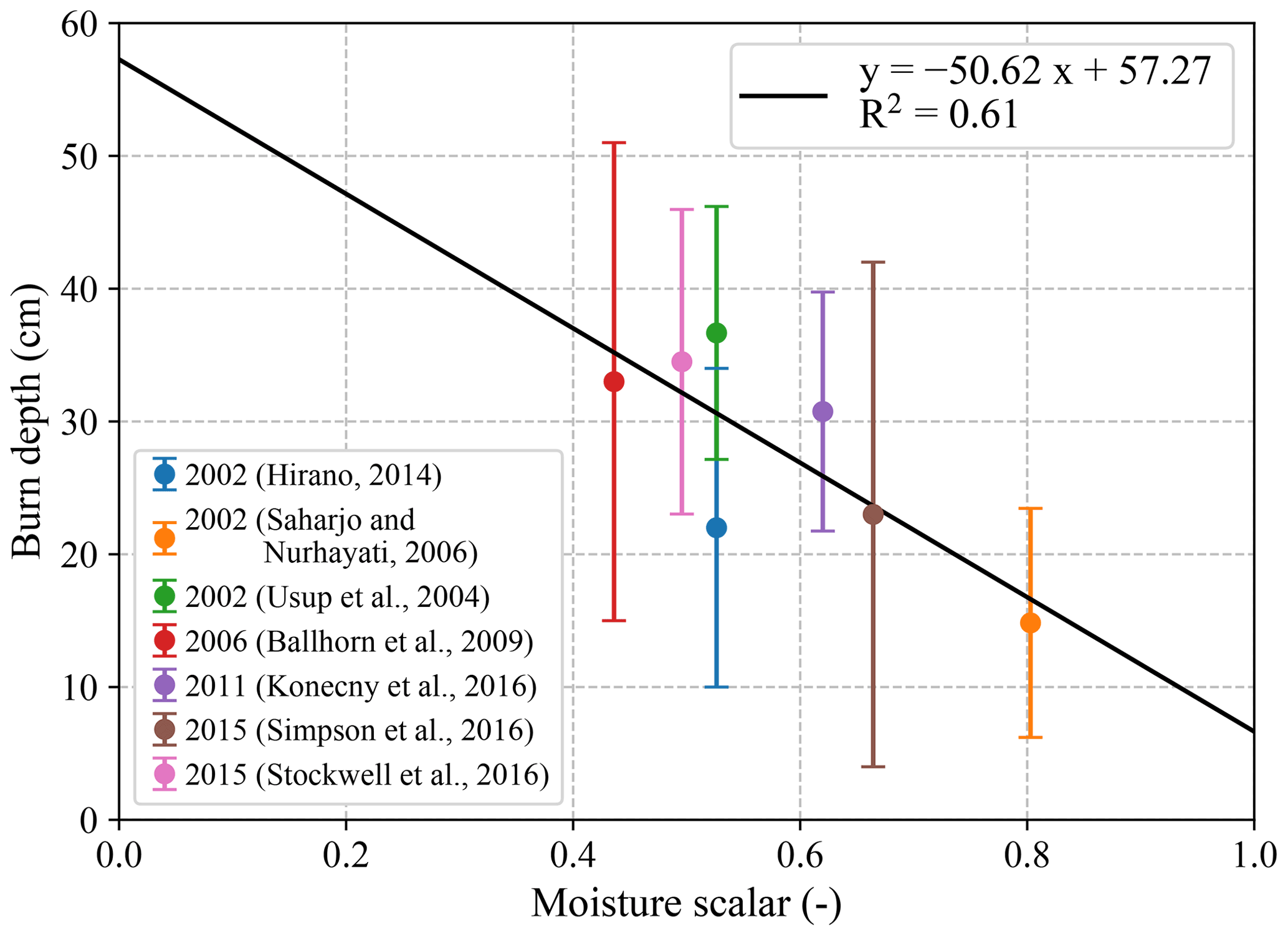
Figure 1Parameterization of burn depth in tropical peatlands (Dburn_tropics) as a function of the soil moisture scalar. The tropical peat burn depth was based on a linear regression function derived from the relationship between field measurements of burn depth and the soil moisture scalar, εSM 0−100 cm. The soil moisture scalar was based on the depth-weighted average volumetric soil water content over the ERA5-land model depths of 0–7, 7–28, and 28–100 cm (Muñoz Sabater, 2019).
The boreal soil burn depth, Dburn_boreal, was based on an empirical linear function:
where εSM 0−28 cm is the soil moisture scalar analogous to Eq. (7) but for the depth-weighted average volumetric soil water content over the ERA5-land model depths of 0–7 and 7–28 cm. This function, with a maximum burn depth of 20 cm, was designed to mimic mean field measurements of burn depth and soil carbon emissions. Even though about 8 % of field entries in the combustion database from NASA's Arctic-Boreal Vulnerability Experiment (ABoVE; Walker et al. 2020) represent deeper burning, a maximum depth of 20 cm was chosen for best correspondence with the average SOC emissions over all field entries in the boreal region. The volumetric soil water content was adjusted to increase variability in areas within the boreal region with consistently high soil moisture such as the Lena River basin. Grid cells with a water content that did not dip below 0.35 m3 m−3 over the full period of 2002–2020 were adjusted to range from 0.25 to 0.45 m3 m−3 based on a linear scaling function (Fig. S1). This adjustment improved belowground combustion compared to measurements from Veraverbeke et al. (2021) in the Lena River basin and from Walker et al. (2020) in boreal North America. The soil organic carbon depth was calculated by dividing the SOC content from the NCSCD dataset by a soil carbon bulk density of 35 kg C m−3. This bulk density was determined as the average bulk density over all field records in the combustion database from Walker et al. (2020). We only modelled boreal soil burning for the boreal forest, sparse boreal forest, tundra, and wetland biomes and excluded boreal croplands and temperate biomes. This way we excluded belowground emissions from agricultural burning, as these fires typically only consume aboveground fuels. Especially in southern Russia, agricultural burning leads to substantial burned area that would otherwise lead to unrealistically high emissions (Hall et al., 2016). The consumed SOC was subtracted from the initial NCSCD stocks so that less carbon was available with each repeated burn, until the SOC pool was fully depleted. In contrast, for the tropical peatlands the carbon pool was assumed to be unlimited, given that peat depths in Indonesia reach several metres (Gumbricht et al., 2017).
Roots were modelled to burn only in the case of fire-related forest loss in combination with soil burning and/or commodity-driven deforestation. In other cases of fire-related forest loss, and in cases of forest loss without fire, roots were modelled to die and eventually become soil organic matter. Fires without forest loss were considered to not affect roots. In the case of soil burning, the root CC was linearly scaled with burn depth to range from 0 % to 10 %. For commodity-driven deforestation, the root CC was linearly scaled with the soil moisture scalar and boosted to range from 20 % to 50 % in order to represent mechanical tree uprooting followed by repeated burning of the slash (Carvalho et al., 1995; Kauffman et al., 1995). In grid cells with both soil burning and commodity-driven deforestation, the latter CC scheme was used, assuming that roots were uprooted regardless of soil burning.
Table 1Overview of datasets used as input for the global model.
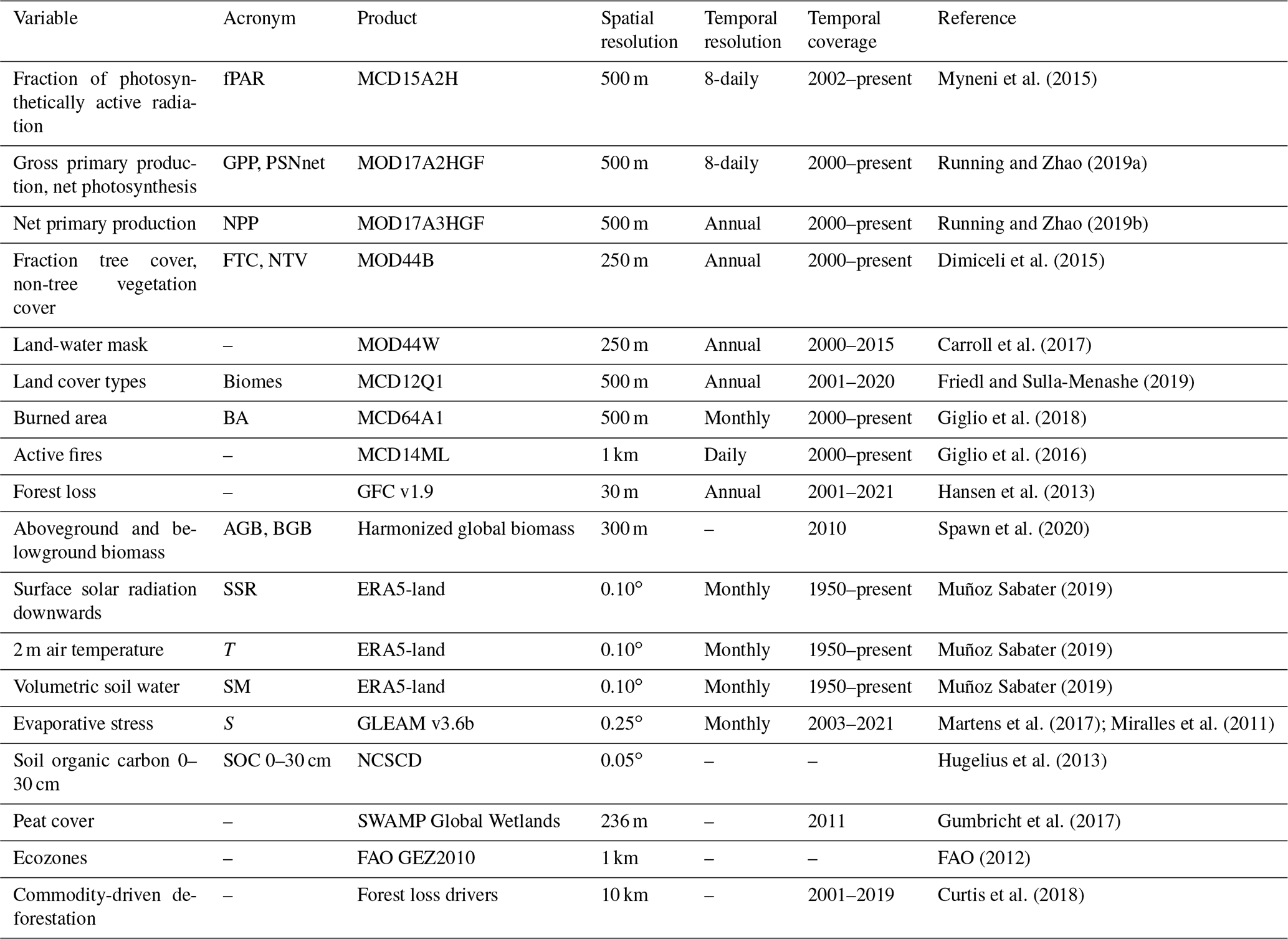
2.2 Input datasets
Model input data primarily consisted of MODIS Collection 6 (C6) satellite observation products with a 500 m spatial resolution, combined with coarser reanalysis meteorology data and other additional datasets focused on forest loss and region masking (Table 1). All datasets were reprojected to the MODIS sinusoidal 500 m grid for model use, using nearest-neighbour interpolation for coarser-resolution datasets and average-based interpolation for finer-resolution datasets. The simulation starting year of 2002 was based on the availability of MODIS data from both the Terra and Aqua satellites. For the calculation of NPP, we used MODIS MCD15A2H fPAR (Myneni et al., 2015) in combination with ERA5-land surface downward solar radiation and air temperature (2 m above surface) (Muñoz Sabater, 2019) and evaporative stress from GLEAM v3.6b (Martens et al., 2017; Miralles et al., 2011) to calculate the temperature and water stress scalars. Since ERA5-land only contains data for land grid cells, large water bodies were complemented with ERA5 data (non-land) (Hersbach et al., 2019) in order to ensure valid data values for coastal grid cells at 500 m resolution. Model NPP was calibrated using MODIS MOD17A3HGF annual NPP. For comparison, monthly MODIS-derived NPP was estimated based on the MOD17 product algorithm and using MODIS MOD17A2HGF monthly gross primary productivity (GPP) and net photosynthesis (PSNnet) (see Sect. S1 in the Supplement). Model NPP was distributed over tree and non-tree vegetation classes using the FTC and NTV data from the MODIS MOD44B Vegetation Continuous Fields (VCF) product (Dimiceli et al., 2015). Soil moisture scalars for the calculation of litter decomposition rates, CC, and burn depth were based on ERA5-land volumetric soil water for the model depths 0–7, 7–28, and 28–100 cm (Muñoz Sabater, 2019). Burned area was derived from the MODIS MCD64A1 burned area dataset (Giglio et al., 2018). Both burned area and additional fire detections from the MODIS MCD14ML active fire product (Giglio et al., 2016) were combined with Landsat 30 m forest loss detections from the Global Forest Change (GFC) product (Hansen et al., 2013) to derive fire-related forest loss at 500 m resolution based on the algorithm from van Wees et al. (2021). Active fire detections were only used where they overlapped with forest loss, using forest loss area as a constraint for burned area. Biome classes were delineated using the MODIS MCD12Q1 land cover type product (Friedl and Sulla-Menashe, 2019). Land cover types from the International Geosphere-Biosphere Programme (IGBP) classification were reclassified to fit model purposes (Table S1; Fig. S2). For the classification of biomes over latitudinal zones, we used the boreal, temperate, and tropical ecozones from the FAO Global Ecological Zones 2010 update (FAO, 2012). The subtropics were categorized under the temperate zone. For water masking we used the MODIS MOD44W land-water mask, defining land as grid cells with at least one land classification over 2000–2015 (Carroll et al., 2017). For boreal belowground fuel consumption, we used the SOC stocks for 0–30 cm depth from the Northern Circumpolar Soil Carbon Database (NCSCD) with a spatial resolution of 0.012∘ (Hugelius et al., 2013). The domain of this dataset is the northern circumpolar permafrost region, which is roughly delineated by mean annual ground temperatures below freezing (Obu et al., 2019). We delineated tropical peatlands using the 236 m binary peatland layer from the SWAMP Global Wetlands Map (Gumbricht et al., 2017), and aggregated these data to derive fractional peat cover at 500 m resolution. Commodity-driven deforestation regions were delineated based on the classification of forest loss drivers by Curtis et al. (2018).
2.3 Model calibration
2.3.1 Calibration of NPP
Model NPP was calibrated against satellite-based annual NPP from the MOD17A3HGF product (Running and Zhao, 2019b) by optimizing the modelled maximum light-use efficiency, εmax, per biome (Table S2). The parameter εmax was determined per biome by minimizing a least-squares function, as proposed by Zhu et al. (2006) and used at a global scale by Liu et al. (2019). The least-squares error, E, is described by
where mi is the reference NPP, and ni is the product of SSR, fPAR, T1, T2, W, and the factor 0.5 (see Eq. 1), multiplied by the function variable y. For each biome, available annual reference NPP values are denoted by i, with a total number of values j. Minimization of the error term E yields the maximum light-use efficiency, z, calibrated for each biome. The comparison was performed for all global land grid cells at 0.05∘ resolution. Model NPP was compared to monthly MODIS-derived NPP estimated using MODIS annual NPP from the MOD17A3HGF product in combination with MODIS monthly GPP and PSNnet from the MOD17A2HGF product (Running and Zhao, 2019a) (see Sect. S1 and Fig. S3 in the Supplement).
2.3.2 Calibration of above- and belowground biomass
After calibration of model NPP, biome-specific turnover rates of the stem and root biomass pools were calibrated to match reference above- and belowground biomass for 2010 from Spawn et al. (2020) (Table S2). The dataset from Spawn et al. (2020) integrates a large collection of previously published biomass maps to provide harmonized above- and belowground biomass maps encompassing all vegetation types. The reference biomass was compared to the average of 2009–2011 model biomass to reduce the impact of interannual variability. The optimal turnover rate for each biome was calculated by solving for the biomass in- and output equations that hold for the model equilibrium state. The reference aboveground biomass was used as the equilibrium state for the stem pool, and the reference belowground biomass was used for the root pool. For the stem pool, the fraction of NPP that it receives is given by
where steminput and NPPstem are the monthly stem biomass input, NPP is the total monthly NPP, and FTC and NTV are the fractions of tree cover and non-tree vegetation cover that distribute NPP over trees and grasses. In CASA, of NPP is allocated to the stem pool. The factor of follows from the relocation of 20 % of stem NPP to the roots, as described in Sect. 2.1. Ignoring disturbance factors such as fire, the output from the stem pool is only based on the natural turnover rate, τstem:
After model spin-up, equilibrium between the stem input and output ensures that
where AGB is the reference aboveground biomass from Spawn et al. (2020). The calibrated τstem for each biome is calculated as the median of τstem over all 500 m grid cells within that biome. For the boreal biomes, calibrated stem turnover rates were found to be notably different between North America and Eurasia. Therefore, the stem turnover rates for these continents were determined separately, avoiding overestimation of aboveground biomass for boreal North America (see Table S2). This could be related to the difference in fire regime between the continents for the boreal region (Rogers et al., 2015), accounted for by different turnover rates.
The root pool NPP input is the sum of the NPP allocated to the roots of trees and the roots of non-tree vegetation, giving
where rootinput and NPProot are the monthly root biomass input. The root turnover rate, τroot, was calculated analogous to Eq. (13) but substituted with NPProot and the reference belowground biomass, BGB. In CASA, of tree NPP and of grass NPP are allocated to the root pool. The factor in Eq. (14) follows from the relocation of 20 % of stem NPP to the roots, as described in Sect. 2.1.
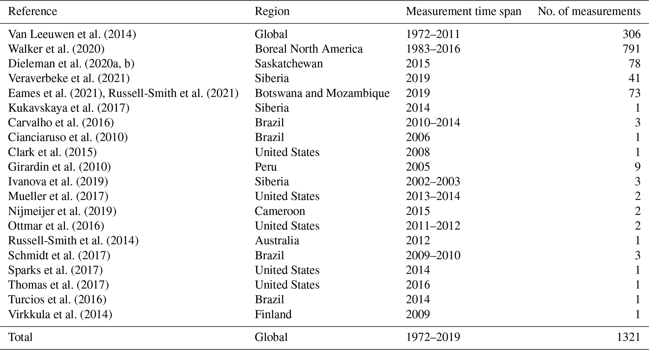
Table 2Overview of reference data for field measurements of fuel load and fuel consumption for producing the updated synthesis database. Each measurement count represents a data entry of fuel load and/or fuel consumption for a measurement-specific set of fuel classes.
2.3.3 Calibration of fuel load and consumption
In the final calibration step, the turnover rates for the remaining aboveground biomass pools (leaf, grass) and the surface litter pools (fine litter, CWD) were tuned individually so that the modelled fuel loads matched measured pools and total fuel loads (Table S2). Next, CC values were tuned so the model matched measured fuel consumption values (Table S3). Field measurements of fuel load and consumption were based on the compiled global database by van Leeuwen et al. (2014), in combination with a large number of additional measurements from more recently published datasets (see Table 2). A link to the updated field measurement synthesis database can be found in the “Data availability” section. These more recent datasets include the collection of field measurements from the ABoVE dataset for boreal North America (Walker et al., 2020), a field campaign in Siberia (Veraverbeke et al., 2021), and a field campaign in Botswana and Mozambique (Eames et al., 2021; Russell-Smith et al., 2021). Furthermore, the original dataset compiled by van Leeuwen et al. (2014) was completely revised by referring back to the source publication of each data entry. In the revision we have resolved several data entry errors, improved the precision of plot coordinates, collected measurement data of individual fuel classes where available, and used other relevant plot information not yet included in the dataset by van Leeuwen et al. (2014). By collecting source data on individual fuel classes, we were able to compare modelled to measured fuel load and consumption for each individual model pool. In the dataset by van Leeuwen et al. (2014) these data were clustered into plot totals, which limited the model comparisons in van Wees and van der Werf (2019) and van der Werf et al. (2017). The precision of the reported plot geographic coordinates was increased to four decimals (0.36′′) where possible, for more accurate plot localization and compatibility with 500 m resolution. Inaccuracies in plot coordinates were solved by selecting a nearby location based on the plot description in the source publication. For example, plots were slightly relocated in cases where the original plot coordinate described a nearby city or when a model grid cell was previously already burned or deforested (depending on the plot's reported fire history).
Further adjustments were made to fully utilize the available field measurement data for model calibration. Entries with a burn date prior to 2002 were compared to 2002 model estimates. In cases where the month was not specified, the month in the middle of the regional fire season was used. For the field data from Walker et al. (2020), only entries with a burn date from 2004 or later were included to ensure consistency of the measurement protocol, correct information on which fuel pools were included in each measurement (Xanthe Walker, personal communication, 2021), and a measurement date within the model period. A selection of entries from Walker et al. (2020) were replaced with values from Dieleman et al. (2020a, b) because fuel class-specific data were available for the aboveground pools (stem, leaf, and fine litter) for these plots. On the contrary, the Walker et al. (2020) dataset only reports total aboveground and belowground pools.
2.4 Simulations
We ran our 500 m resolution fire emissions model for the 2002–2020 period at a monthly time step. The model required a spin-up in order to stabilize carbon pools. In order to reduce required computational resources, the spin-up was divided into a 300-year annual phase to stabilize pools with slow turnover rates (e.g. stems) and a 30-year monthly phase to introduce monthly variability. Both phases were based on the 2002–2004 climatology of input data to represent the early period of vegetation cover while reducing the influence of interannual variability, except for the biome data and burned area data. For the biome data, the majority biome in the 2001–2003 period was used in order to reduce interannual variability and to reduce the influence of land conversion (e.g. deforestation) during the first simulation years. For the burned area data, different climatologies were used for biomes with a short or long fire return interval. For biomes that burned relatively frequently on average, namely shrublands, savannas, grasslands, and croplands, the 2002–2020 climatology was calculated per 500 m grid cell. For biomes with a longer fire return interval (generally high tree cover), the burned area during the spin-up was set to zero, and instead the biome-specific turnover rates (Table S2) and tree and non-tree vegetation cover fractions implicitly accounted for the fire regime. For these biomes the time-averaged burned area was generally <1 % of a 500 m grid cell, allowing for approximation by zero. Setting the burn climatology to zero for these biomes minimized underestimation of local biomass before the actual fire event. For the annual spin-up phase, monthly turnover rates were converted to annual rates via
where τannual and τmonthly are the turnover rates per year and month, respectively. During the spin-up, processes related to forest loss and belowground fire were switched off because of their long-term impact.
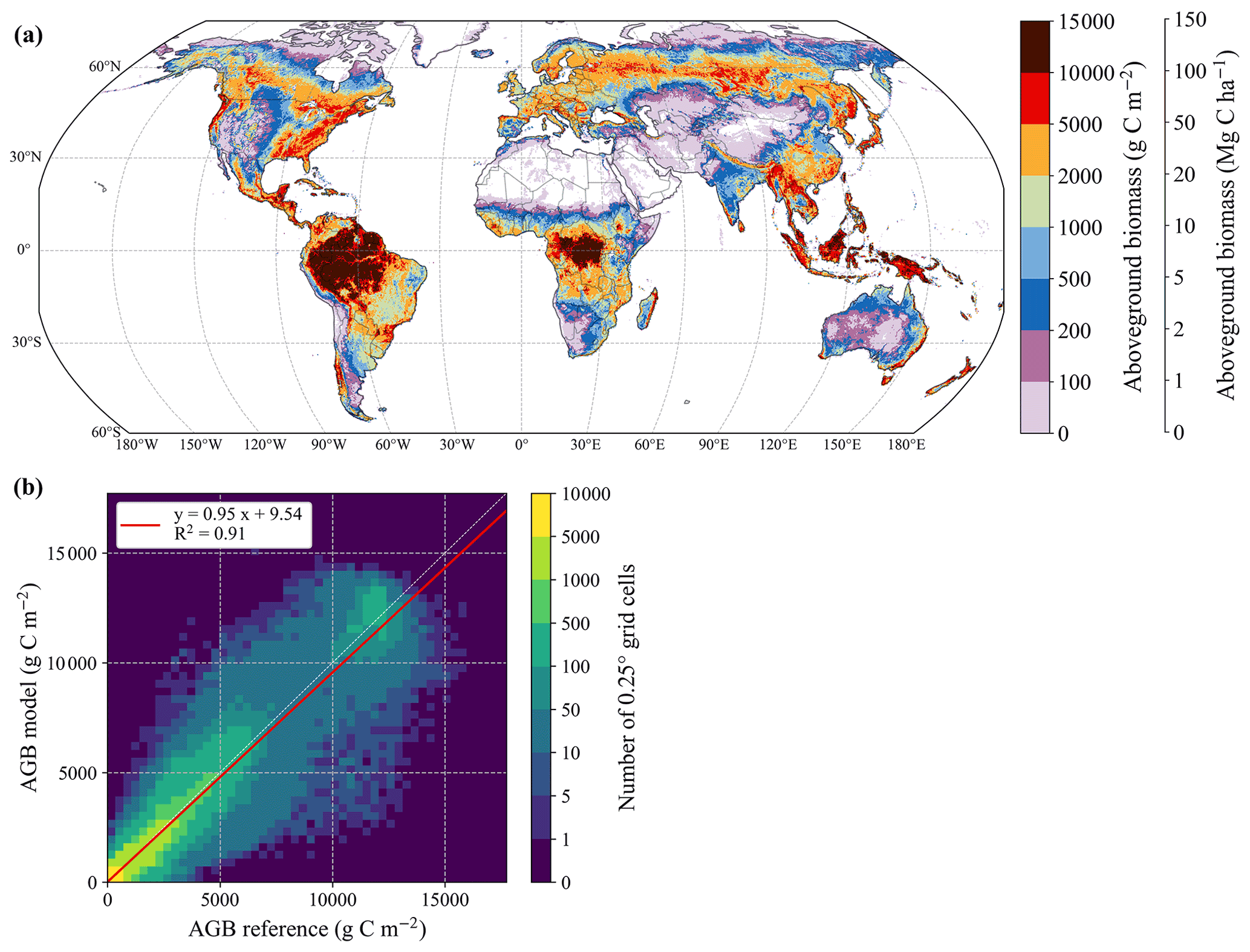
Figure 2(a) Modelled aboveground biomass (AGB) averaged over 2002–2020 and (b) comparison of modelled versus reference aboveground biomass from Spawn et al. (2020), at an aggregated 0.25∘ grid cell level. Model AGB comprises the stem, leaf, and grass model pools and does not include litter pools. Panel (a) has been aggregated to 0.25∘ for display.
3.1 Model optimization
Average annual model NPP was 57±1 (±1σ interannual variability; IAV) Pg C yr−1, compared to 58±2 Pg C yr−1 for MODIS and 63±1 Pg C yr−1 for GFED4(s) (from 2002 to 2016). The seasonal pattern was largely in agreement with MODIS (Fig. S3). The overall effective light-use efficiency (εeff) for our model was 0.29 g C MJ−1 (Table S2). Optimized stem turnover rates ranged from about 40 years in some low-tree cover biomes up to 82 years for boreal forests and tundra, with a global average of 48 years (Table S2). Effective average root turnover rates ranged from 1 year in temperate croplands to almost 10 years in the boreal tundra. Based on the biome-dependent stem and root turnover rates, the spatial pattern of above- and belowground biomass aligned well with the reference data (R2=0.91 for stem, R2=0.82 for roots) from Spawn et al. (2020) (see Fig. 2 for aboveground and Fig. S4 for belowground). As a result, total global aboveground biomass was 284 Pg C, and belowground biomass was 121 Pg C, identical to the values reported by Spawn et al. (2020). The total biomass of 404 Pg C is slightly higher than another independent estimate of 380 Pg C reported by Xu et al. (2022). Spatial differences in aboveground biomass between the model and the reference map were largely the result of the reliance on MODIS-based FTC and NTV for the spatial distribution of biomass in the model. For example, tree biomass for the western part of the Congo Basin tropical rainforests was underestimated as a consequence of low MODIS FTC in this area (Figs. 2 and S5a). For belowground biomass, the largest areas with discrepancies were also found in Africa. For some savannas across Kenya and Somalia, the reference belowground biomass density locally was greater than 4000 g C m−2, which was not reproduced by the model (Figs. S4 and S5b). However, because belowground burning is not occurring in those areas, this has no impact on fire emissions.
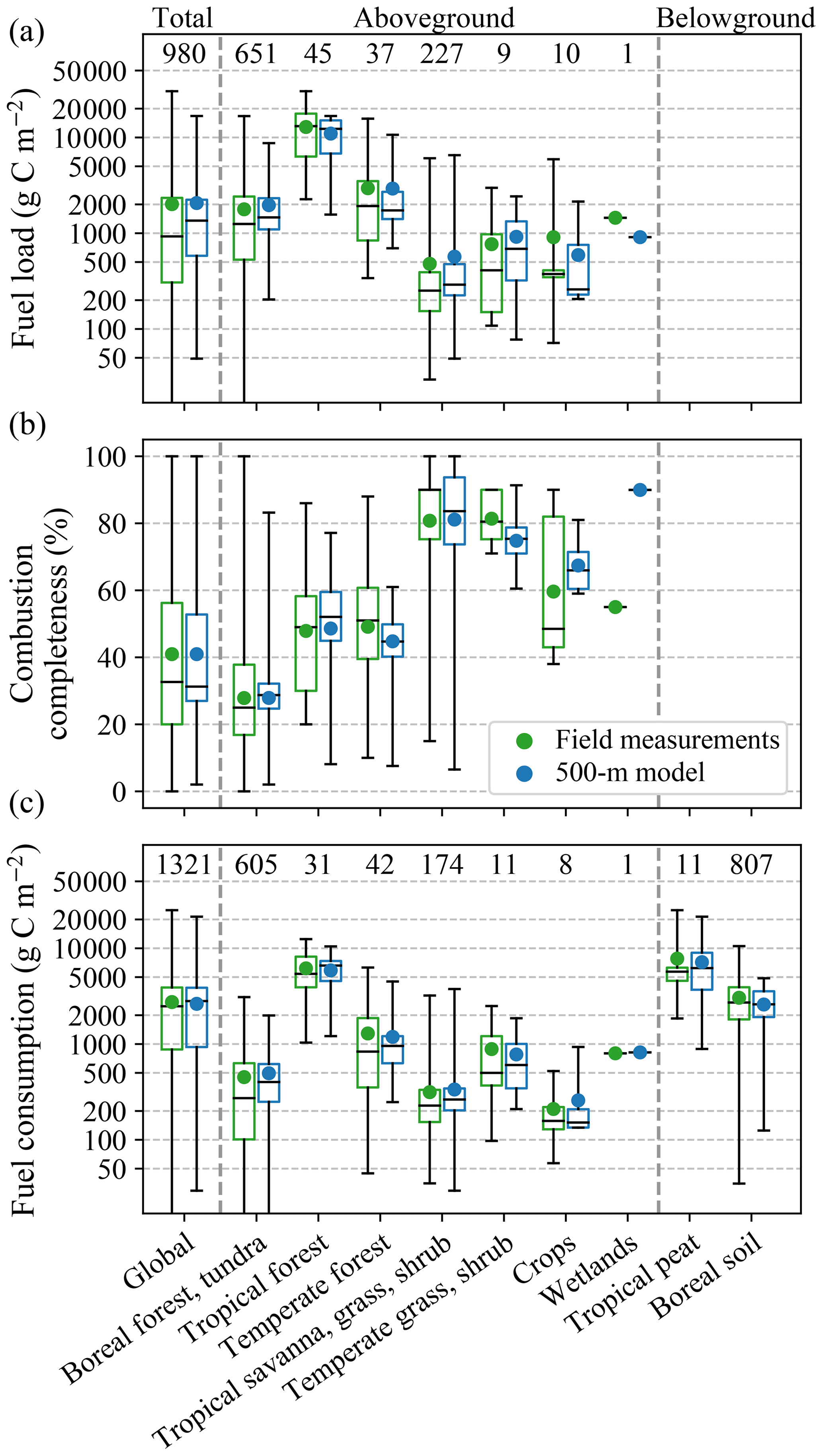
Figure 3Comparison of field measurements of (a) fuel load, (b) combustion completeness (CC), and (c) fuel consumption versus model estimates for all field data (Table 2), grouped per biome class. The number of measurement records included is given above each box plot. Aboveground and belowground fuel classes are grouped separately. Belowground fuel classes (tropical peat and boreal soil) are only reported for fuel consumption measurements because our model relied on static SOC density maps for calculating soil fire emissions (see Sect. 2.1.3). Global values are for the total measured fuel available, which in the case of (a) and (b) are aboveground values and for (c) are the sum of above- and belowground for each measurement record. Note that the number of fuel consumption measurements for the individual biomes does not sum to the global total number of sites (1321) because measurement records with both aboveground and belowground values are being counted as one record in the global class. The y axes of panels (a) and (c) are logarithmic, and the y axis of panel (b) is linear. Box plot whiskers give the range of data.
Biome-averaged fuel load and fuel consumption agreed well with field measurements (Fig. 3) as a result of optimizing the turnover rates and CC per biome and fuel class (Fig. S6). Even though the mean value and variability were optimized for each biome and fuel class, the model was not always able to capture the full variability among field measurements. Particularly for the data from Walker et al. (2020), representing 60 % of all field data entries (Table 2), the model was often not able to represent individual measurements. When omitting the data entries from Walker et al. (2020), the model correlated well with individual field measurements of fuel consumption (R2=0.73). However, by including the data from Walker et al. (2020), the correlation was much lower (R2=0.28), likely as a consequence of fine-scale variation in site drainage regulating fuel consumption in boreal forests that was not resolved at a 500 m spatial resolution (Walker et al., 2020).
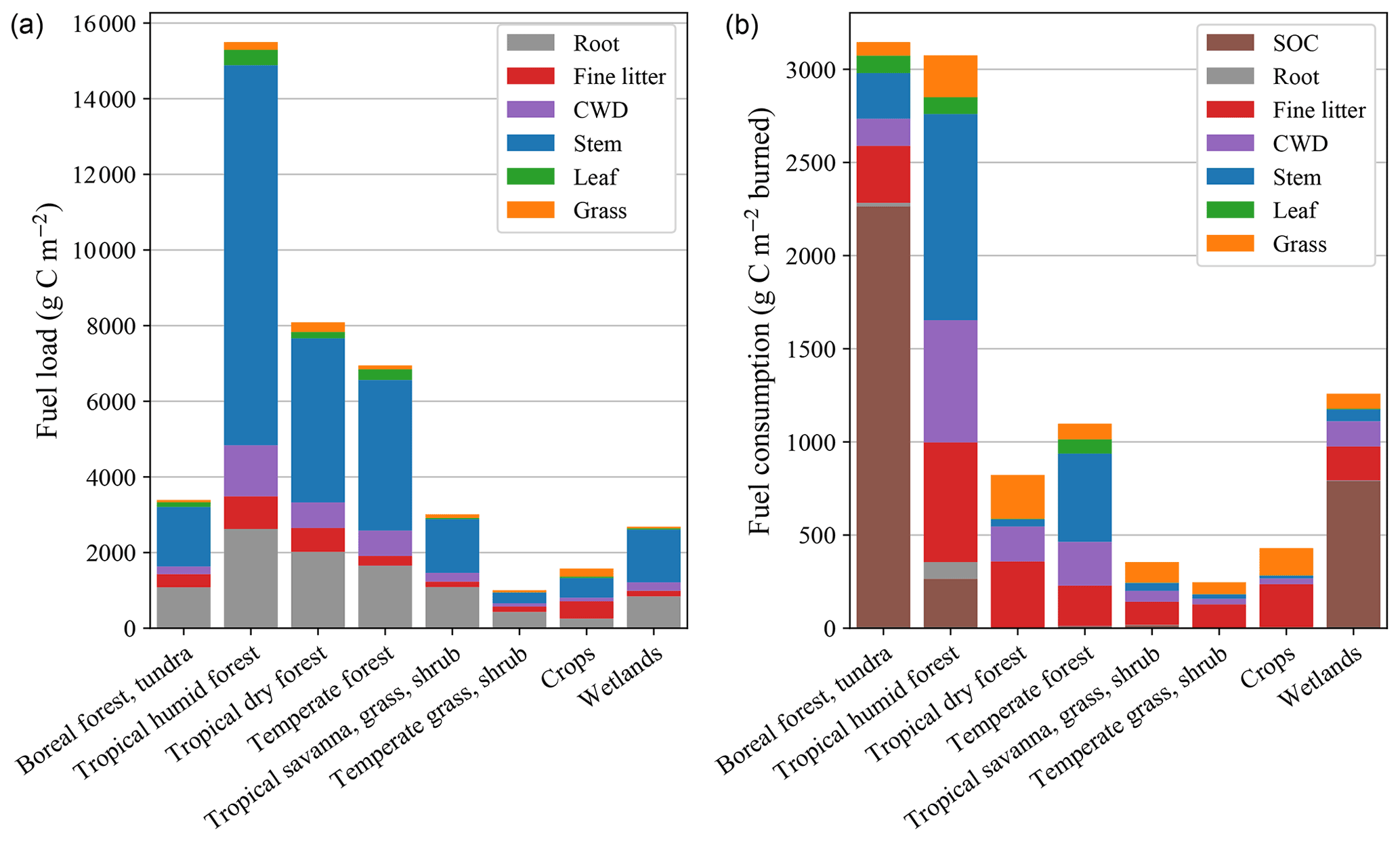
Figure 42002–2020 average (a) fuel load and (b) fuel consumption per biome. Bars are subdivided in model biomass and litter pools. Because of the use of static SOC maps, panel (a) does not include soil organic carbon fuel loads.
The average distribution of biomass over roots, stems, and leaves in forest biomes was 26 %, 69 %, and 4 %, respectively (Figs. 4a, S7a and c). For savanna, shrubland, grassland, and cropland biomes combined, this was 41 %, 51 %, and 8 % on average. These ratios were largely in accordance with field-measured distributions as synthesized by Poorter et al. (2012). Fine litter and CWD each constituted on average 10 % and 11 % of total aboveground (live and dead) plant material, respectively, for all biomes combined. For emissions, the fine litter and CWD pools played a much larger role, representing about half of all aboveground fuel consumption for all biomes (Figs. 4b, S7b and d). In forest biomes, the consumption of stems was the following major contributor, dependent on the amount of fire-related forest loss, whereas in low-tree-cover biomes, the consumption of grasses played an important role.
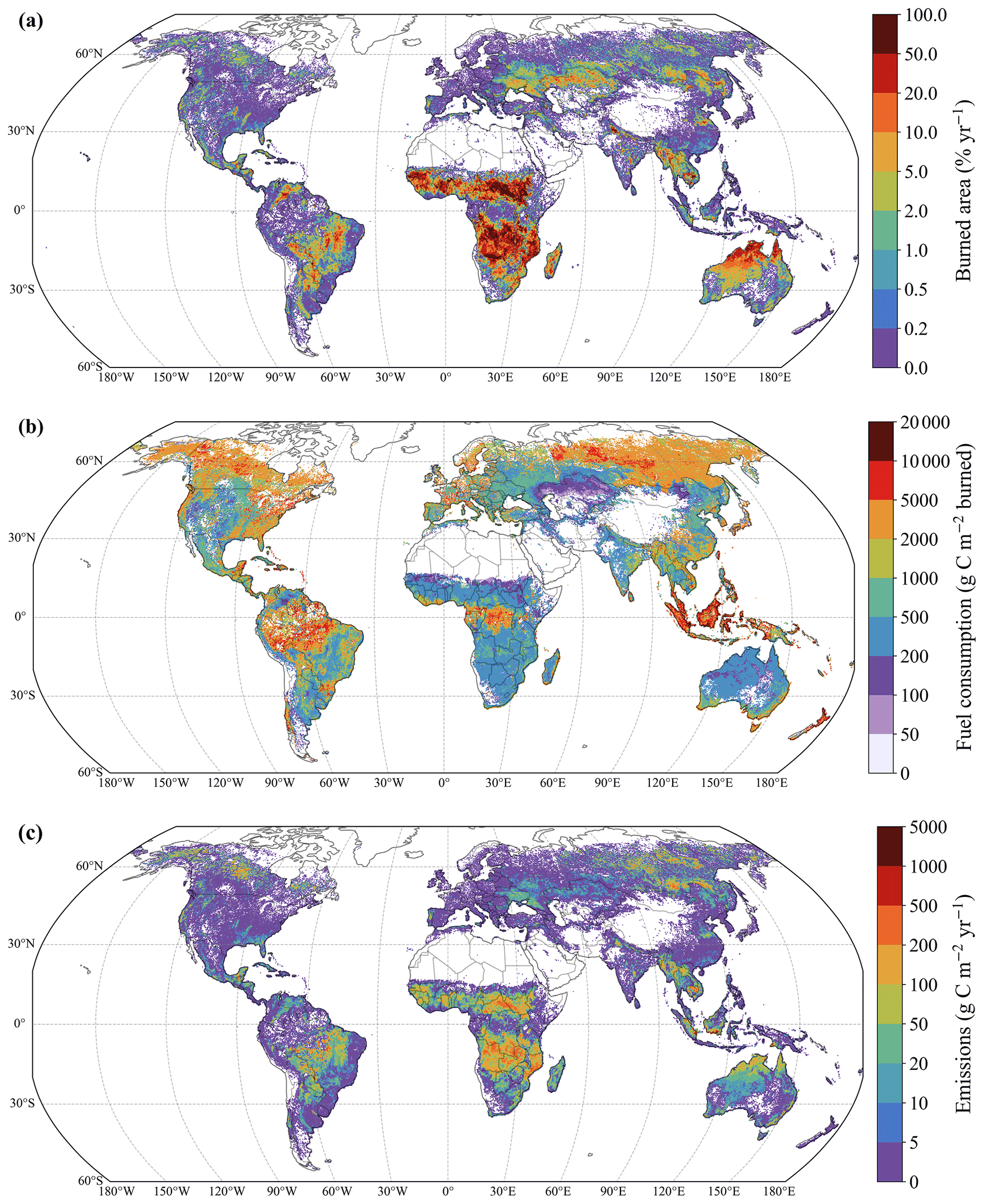
Figure 5Global annual (a) burned area, (b) fuel consumption, and (c) emissions, averaged over 2002–2020. Burned area displayed in panel (a) is the total burned area derived from combining the MODIS MCD64A1 product and additional fire-related forest loss burned area from active fire detections that overlap forest loss. Maps are aggregated to 0.25∘ for display.
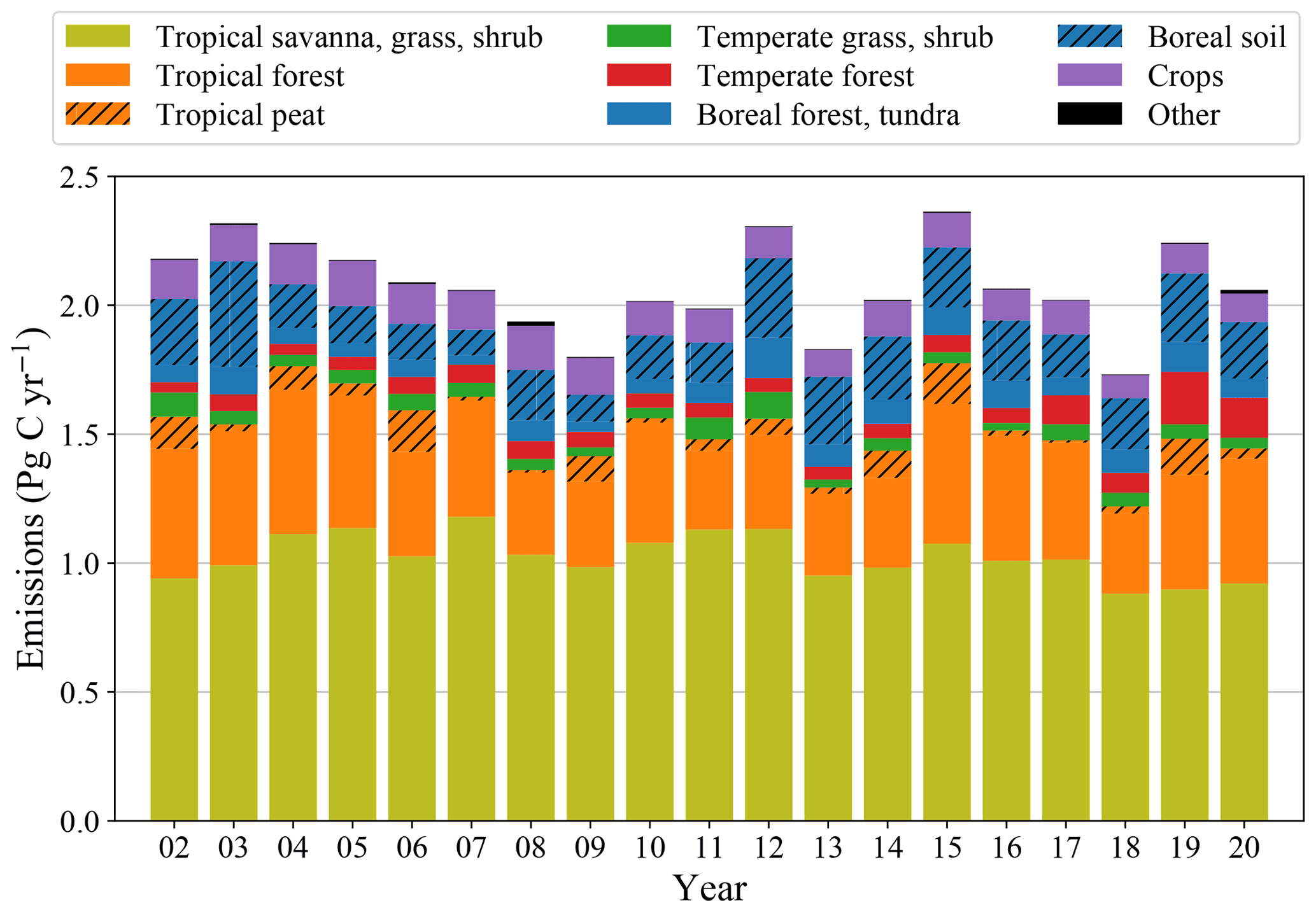
Figure 6Global annual emissions for 2002–2020 based on the 500 m model. Bars are subdivided into biomes, with belowground emissions in two separate classes (tropical peat and boreal soil).
Table 32002–2020 average fuel load, fuel consumption, burned area, and emissions per GFED region. Fuel load and fuel consumption are reported in fuel groups of aboveground biomass (AGB; stem, leaf, and grass model pools), surface litter (fine litter and CWD model pools), belowground biomass (BGB; root model pool), and soil organic carbon (SOC). Fuel consumption, burned area, and emissions from GFED4s are reported for comparison. Field averages are based on the average fuel consumption over the field measurement entries located within a GFED region. The number of field plots involved in each field average is given in parentheses.
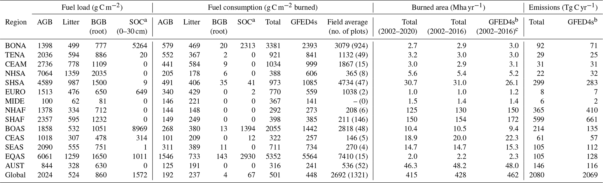
a Soil organic carbon (SOC) fuel load and fuel consumption values
are only considered for the boreal region and tropical peatlands in
Indonesia, Malaysia, and the Pantanal and Paraná Delta in South America,
delineated by the static boreal SOC map from the NCSCD database
(Hugelius et al., 2013) and tropical peatland layer from the
SWAMP Global Wetlands Map (Gumbricht et al., 2017) (see
Sect. 2.1.3). SOC is non-zero for TENA and CEAS because definitions of the
southern border of the boreal region differ between
Hugelius et al. (2013) and the GFED regions from
van
der Werf et al. (2017). Tropical peatland SOC fuel loads are given for 0–30 cm depth for consistency with the boreal SOC stocks and based on a constant
carbon density of 54 kg C m−3.
b GFED4s emissions cannot be directly compared to the 500 m
model estimates, as they are based on different amounts of burned area (see
Sect. 4.2).
c GFED4s burned area is only available up to 2016 due to
dependency on MCD64A1 Collection 5.1 burned area, which was discontinued
after 2016. GFED4s emissions for 2017–2020 are released as a beta product
and based on a parameterization using MODIS active fires from the MCD14
product (Giglio et al., 2016). For
comparison, we also give the burned area from the 500 m model for the
2002–2016 period.
3.2 Fuel consumption and emissions
Global average carbon emissions from fire for 2002–2020 were 2.1±0.2 Pg C yr−1 (Figs. 5 and 6; Table 3). These emissions resulted from 415±42 Mha yr−1 of burned area, of which 410±43 Mha yr−1 originated from the MODIS MCD64A1 product and 5.4±1.2 Mha yr−1 (uncertainty range =2.5–8.3 Mha yr−1) from forest loss area overlapped by active fire detections calculated as part of the fire-related forest loss module. Global averaged fuel consumption was 501 g C m−2, of which almost half originated from the surface litter pools. In the boreal region and the tropical peatlands of Equatorial Asia, fuel consumption was dominated by the SOC pool. Notably, fuel consumption in the boreal region transitioned abruptly at 60∘ E due to the domain limits of the northern circumpolar permafrost region from the NCSCD dataset, related to a temperature transition at the Ural Mountains (Fig. 5b). Emissions were largest in 2015 at 2.4 Pg C yr−1 and smallest in 2018 with 1.7 Pg C yr−1 (Fig. 6). Of all emissions, 76 % originated from the tropics, with 1072 Tg C yr−1 from tropical savannas, grasslands, and shrublands and 445 Tg C yr−1 from tropical humid and dry forests. The temperate regions accounted for 9 % of global emissions, with 75 Tg C yr−1 from temperate forests and 54 Tg C yr−1 from temperate grass- and shrublands. Finally, the boreal region accounted for 14 % of global emissions, or 291 Tg C yr−1, of which 209 Tg C yr−1 (72 %) was the result of belowground burning of SOC. In comparison, tropical peatlands emitted 64 Tg C yr−1 (3 % of global emissions), with considerably more annual variability. Only in 2006 were SOC fire emissions from tropical peatlands larger than those from the boreal region. Cropland emissions from tropical, temperate, and southern boreal regions were 136 Tg C yr−1 in total, with most emissions (79 Tg C yr−1) from the tropics, followed by temperate croplands (56 Tg C yr−1).
Fire-related forest loss accounted for 10.9±2.9 Mha yr−1 (uncertainty range =8.1–13.7 Mha yr−1; 1.9 %–3.3 % of global total) of burned area, resulting in emissions of 541±144 Tg C yr−1 (uncertainty range =390–673 Tg C yr−1; 19 %–32 % of global total) (Fig. S8). This illustrates how fuel consumption rates are more than a factor of 10 higher on average in the case of fire-related forest loss (4966 g C m−2 burned) as compared to fire without forest loss (381 g C m−2 burned). The IAV in emissions from fire-related forest loss was 144 Tg C yr−1 and thus an important contributor to the interannual variability in global emissions. On a regional scale, the contribution of fire-related forest loss to total fire emissions varied widely, from close to 0 % in most savannas to 100 % in some forested areas (Fig. S9). The latter situation primarily occurred in closed-canopy forests with relatively small-scale fires, such as the interior tropical rainforests and temperate forests with minor fire activity. In these cases, fire-related forest loss was often only captured by MODIS active fire detections and not in the MCD64A1 burned area product (Fig. S9c) (van Wees et al., 2021).
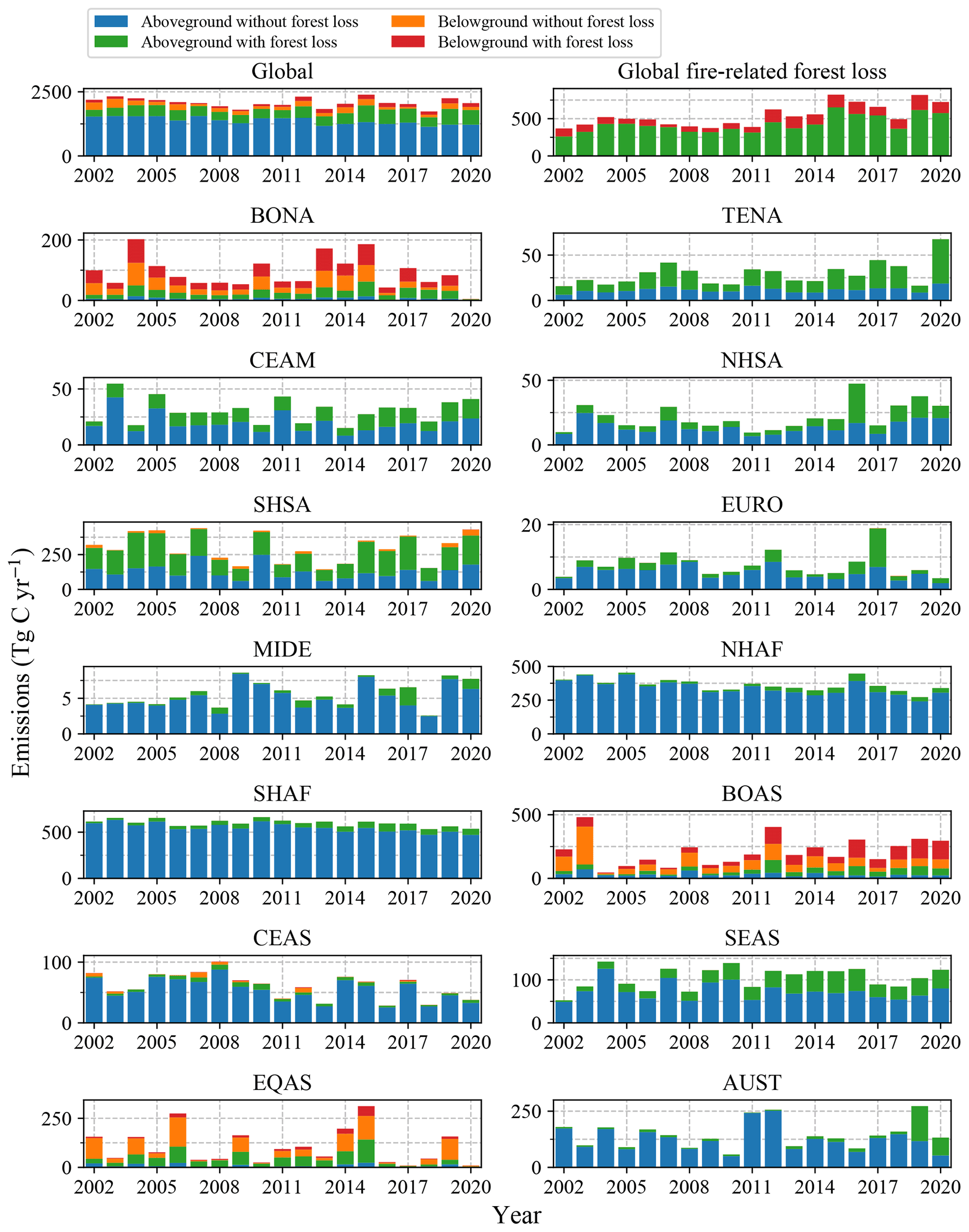
Figure 7Annual 2002–2020 emissions for the global total, global fire-related forest loss, and the 14 GFED regions. Bars are subdivided into aboveground and belowground emissions and into fire without forest loss and with forest loss (i.e. fire-related forest loss).
Emissions from the burning of SOC were considerable, accounting for 281±93 Tg C yr−1 (13±4 % of global total). Both for the boreal region and equatorial Asia these emissions represented the majority of total emissions (Fig. 7). For the boreal region, SOC fire emissions accounted for between 66 % and 79 % of total annual emissions, a fraction that was relatively stable over years. In contrast, the relative share of peat fires to total emissions for equatorial Asia varied substantially from year to year, with a minimum of 17 % in 2008 and a maximum of 75 % in 2019.
We have produced global fire emissions estimates based on fuel load modelling at an unprecedented spatial resolution of 500 m. Our approach was based on the modelling framework that was built for a case study for sub-Saharan Africa (van Wees and van der Werf, 2019) and has been expanded to global extent with, among other refinements, an updated calibration procedure, a fire-related forest loss module, and parameterizations for SOC emissions. While the framework for modelling NPP and the turnover rates of fuel pools remained similar, the calibration of most of the underlying parameters has been automated and further extended to be biome-specific to ensure optimized model performance. CC ranges have also been changed to be biome-specific, considerably improving the representation of fuel consumption as compared to field measurements (Table S3; Figs. 3 and S6). With a global extent at 500 m resolution, the model required additional model complexity to represent all biomes and fire types. This included representing deforestation mechanisms in the Amazon, peat fires in Indonesia, and belowground fuel consumption in boreal forests.
4.1 Comparison to field measurements
Modelled fuel load and consumption were calibrated to match individual field-measured pools to constrain the amount of fuel stored and emitted per pool. Van Wees and van der Werf (2019) showed that the comparison of field plots to 500 m model grid cells reduced the representation error as compared to calibration at 0.25∘ resolution in GFED4(s). In general, the model performed well in reproducing measured averages and variability for individual biomes and pools (Figs. 3 and S6). Nonetheless, model variability was generally lower, and discrepancies for individual measurements could still be large. However, this is not surprising considering that many of the specific field conditions reported in field studies were not explicitly part of the modelling framework. The impacts of different field conditions are often among the main focal points of field studies (e.g. Cianciaruso et al., 2010; Walker et al., 2020), influencing fuel conditions and fire behaviour. This includes, for example, the time since last burn, local fallow and/or grazing conditions, forest management approaches, site drainage conditions, and vegetation species composition, all of which may influence fine-scale variability in fuel consumption and fire severity. Furthermore, for some of the field data entries, the exact measurement location or time was unknown, and/or the measurement was conducted before the start of the model period in 2002. Optimal direct comparison between field data and models would require 20–30 m satellite data and models, as ultimately 500 m resolution is still too coarse to represent the sub-500 m heterogeneity found among field plots. This was well-illustrated in boreal North America, for which the large number of available measurements demonstrate the large variability in fuel loads and consumption among field plots. Nonetheless, even models specific to boreal North America that partially or fully incorporated 30 m resolution predictors of fuel load and consumption still underrepresented the heterogeneity among fuel consumption as observed by field measurements (Dieleman et al., 2020a; Veraverbeke et al., 2015; Walker et al., 2018). This shows that besides including the best-available spatio-temporal predictors, additional vegetation and combustion process simulation may be required for improved estimates. Additional field measurements in the tropical and temperate regions might reveal that such added model refinement is also required for other biomes. Even though available biomass and litter pools are constrained with biome averages, additional representation of spatial variability in CC is required for both aboveground and belowground fuel classes.
Since the release of the field measurement synthesis by van Leeuwen et al. (2014), a substantial number of new field observations have become available, increasing the number of field data entries in our updated synthesis database to a total of 1321 (Table 2). Most new field data became available for the boreal region as a result of a synthesis effort sponsored by NASA's ABoVE campaign for boreal North America (Dieleman et al., 2020a, b; Walker et al., 2020) and additional field campaigns in Siberia (Kukavskaya et al., 2017; Veraverbeke et al., 2021). Furthermore, recent field campaigns in Africa have roughly doubled the available measurements for the savanna biomes (Eames et al., 2021; Russell-Smith et al., 2021). The additional field data better constrain fuel consumption globally. For the boreal region this reframes the consensus on the amount of belowground consumption of SOC in boreal fires. Boreal forest fire emissions were considerably higher than in GFED4s, mainly due to higher fuel consumption of soils, as revealed by the recent measurements from Walker et al. (2020) (Figs. 8 and S10). With climate change, the combination of increased fire activity and permafrost degradation could further increase the share of the boreal region in global fire emissions (Veraverbeke et al., 2021).
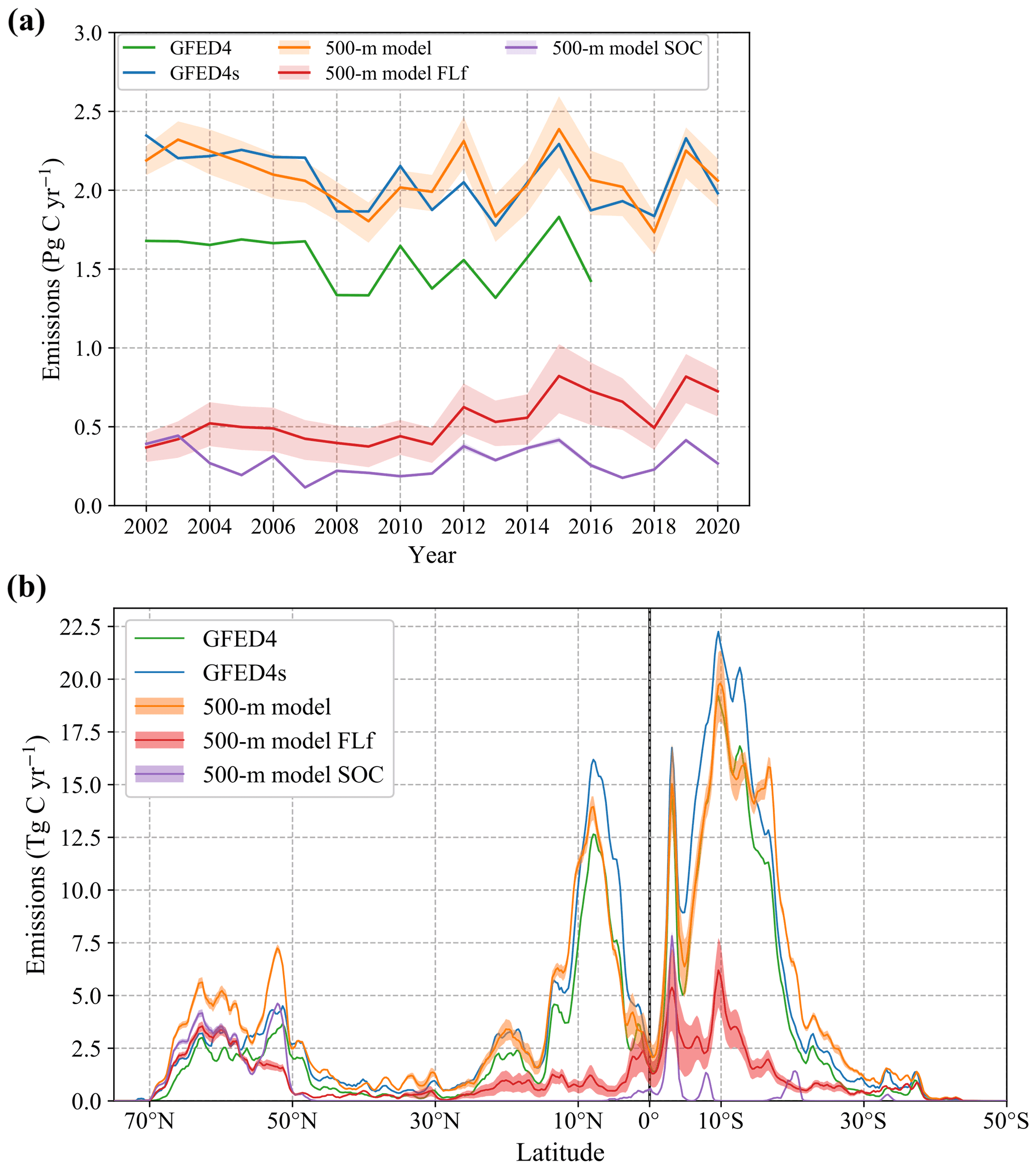
Figure 8Annual global emissions for the 500 m model for 2002–2020 versus GFED4s for the same time period and GFED4 for 2002–2016 as (a) time series and (b) latitudinal total emissions. Contributions to 500 m model emissions from fire-related forest loss (FLf) and SOC burning are displayed separately. Note that these subcategories partly overlap: fire-related forest loss emissions include part of SOC burning emissions and vice versa. Transparent bands around estimates show the range between minimum- and maximum-probability fire-related forest loss. All lines in panel (b) are based on 0.25∘ aggregated data and smoothed using a moving-average filter with a window size of four grid cells, i.e. 1∘ latitude.
By revising the available field data, we were able to compare individual fuel pools at a global scale, allowing for improved constraints of fuel load and consumption for each model pool. The model results show that about half of global emissions originate from the fine litter and CWD pools, stressing the importance of representing these pools correctly. At the same time, fine litter and CWD fuel loads are probably the most difficult to estimate on a global scale due to the difficulty in using satellite remote sensing to measure these fuels on the ground and below the canopy. Recent developments in the estimation of aboveground biomass using emergent technologies such as lidar are an important prerequisite for improved fuel models (Duncanson et al., 2022), but better constraints on litter pools may require yet different approaches, such as local-scale multispectral drone observations (Eames et al., 2021). Until those difficulties are resolved, field data on pool-specific fuel loads and consumption will continue to be vital for informing models such as ours.
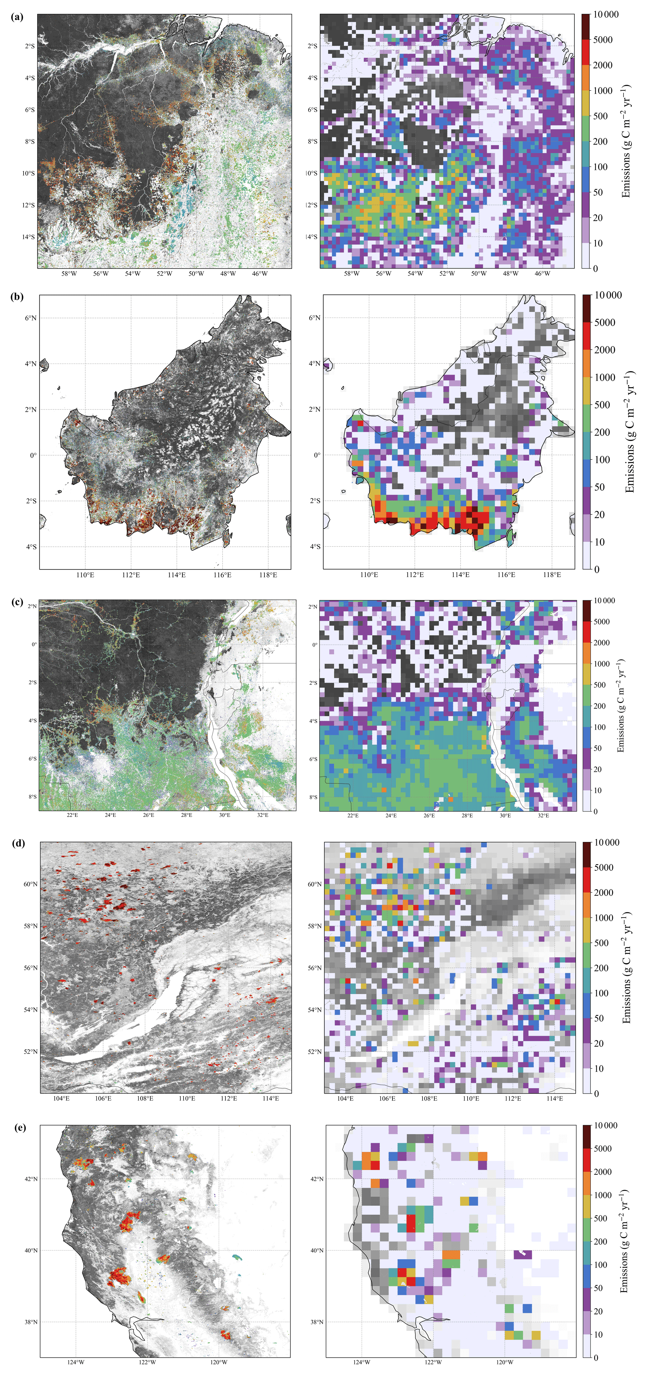
Figure 9Regional maps of annual emissions from the 500 m model (left column) and GFED4s (right column; with a model resolution of 0.25∘). (a) Deforestation in the south-eastern part of the Brazilian Amazon and the transition to savanna fires in the Brazilian Cerrado for 2004. (b) Deforestation on Borneo for 2006, including fires in drained peatlands (primarily on the southern coast). (c) Savanna fires and deforestation in the south-eastern part of the Congo Basin for 2016. (d) Boreal wildfires north and east of Lake Baikal in Siberia for 2017. (e) Temperate wildfires on the west coast of the United States for 2018. Greyscales show fractional tree cover.
4.2 Comparison to GFED4(s)
Our estimate of global fire emissions of 2.1±0.2 Pg C yr−1 is higher than the 1.5±0.2 Pg C yr−1 for GFED4 but similar to 2.1±0.2 Pg C yr−1 for GFED4s (Figs. 8, S10 and S11). Differences between the model estimates can be attributed to differences in both the amount of burned area and the modelled fuel consumption and emissions at finer spatial resolution (Fig. 9). GFED4 burned area was based on the MODIS MCD64A1 Collection 5.1 product, which mapped less global burned area than the Collection 6 product used in our study. For the 2002–2016 time period, Collection 6 burned area was 26 % higher than Collection 5.1, with increases in most regions (Giglio et al., 2018). With the inclusion of small-fire burned area in GFED4s, 37 % additional burned area was added to Collection 5.1 (Randerson et al., 2012), resulting in 11 % more global total burned area than Collection 6. By including fire-related forest loss based on active fire detections in our model, we added an additional 3 % to Collection 6 burned area, with a strong bias towards high-fuel-consumption fires. As a result, the burned area in our model (428 Mha yr−1) was 8 % lower than GFED4s (462 Mha−1) for the 2002–2016 period, while global emissions from our model and GFED4s differed by only 1 % (Table 3).
Other factors that explain the difference in emissions between our 500 m model and GFED4(s) can be summarized by differences in modelled fuel consumption, which follow from differences in the modelling framework, better-constrained model calibration due to additional field data, and more fundamental differences following from the higher spatial resolution of our model. Global average fuel consumption for our model was 501 g C m−2, which is 12 % higher than the 448 g C m−2 in GFED4s and counteracted the 8 % lower burned area. The higher fuel consumption could mainly be attributed to more combustion of SOC in the boreal region. This increase primarily originates from algorithm changes regarding belowground fuel consumption, based on improved measurements. Notably, in regions with little burned area (e.g. Middle East, Europe), fuel consumption was also considerably higher as a result of more resolved fuel consumption heterogeneity at 500 m resolution. As described by van Wees and van der Werf (2019), the higher model resolution of 500 m also plays an important role by (1) reducing the representation error between model grid cells versus field-measured data, which in turn impacts model calibration, (2) removing the non-linear propagation of aggregated input datasets, (3) reducing biome misclassification (edge effects whereby multiple biomes within a grid cell are given one summary value), and (4) improving fuel-tracking in case of repeated burns. In combination with differences in the modelling framework and additional field data for calibration, this mainly resulted in higher fuel consumption in the interior tropical forests and boreal forests and lower emissions towards the edges of these forest biomes, as compared to GFED4s (Fig. S11). Higher fuel consumption for the 500 m model in the interior tropical forest, but also some temperate forests such as in the south-eastern United States, is largely explained by the additional burned area from fire-related forest loss based on active fire detections in regions with fires too small to be detected by the MODIS 500 m burned-area algorithm. Other positive and negative differences between models can mainly be explained by a combination of differences in the model calibration per biome and increased spatial variability in fuels at finer resolution.
4.3 Fire-related forest loss
Here we estimated fire-related forest loss emissions of 0.54±0.14 Pg C yr−1 (uncertainty range =0.39–0.67 Pg C yr−1). By combining the 30 m annual forest loss data with monthly 500 m fire data, fire-related forest loss emissions could be distributed over months at 500 m resolution. The benefits of satellite-derived information on the spatial extent of forest loss and the timing of fire activity allowed for a more constrained emissions estimate compared to the previously used mortality scalar in GFED. Despite these benefits, there are several caveats to this approach.
First, the underlying forest loss time series is inconsistent over time, inhibiting trend analysis (Hansen et al., 2013; van Wees et al., 2021). The forest loss detection algorithm developed by Hansen et al. (2013) was different for the 2001–2012, 2013–2014, and 2015–present time periods due to the introduction of Landsat-8 OLI images from 2013 onwards and changes in the detection algorithm. These changes led to improved detection efficiency and an artificial increasing trend in the forest loss time series. Therefore, the increase in fire-related forest loss emissions (+0.02 Pg C yr−2; p<0.01) as shown in Fig. 8a should be interpreted with caution. We did not find any significant trends in fire-related forest loss emissions for the individual 2002–2012, 2013–2014, and 2015–present periods. We did find a significant negative trend in fire emissions unrelated to forest loss of −0.03 Pg C yr−2 (p<0.01) for 2002–2020 and a trend of −0.03 Pg C yr−2 (p=0.03) for 2002–2012, in line with an observed decline in global burned area (Andela et al., 2017). This decline is counteracted by the increase in fire-related forest loss emissions, which disproportionally affects global total emissions due to the relatively high fuel consumption of fires related to forest loss. Despite these limitations, high global fire emissions in the years 2012, 2015, and 2019 can still largely be explained by high fire-related forest loss (Fig. 8a). Another approach is required to disentangle emission trends resulting from the decline in global burned area and an opposing increase in forest fire emissions (Zheng et al., 2021).
A second caveat to the fire-related forest loss module follows from the discrepancy in burned area from the fire-related forest loss algorithm as compared to MCD64A1 Collection 6. Originating from the 30 m forest loss data, the fire-related forest loss area is a fraction of a 500 m grid cell, whereas the MCD64A1 burned area is binary at 500 m. Therefore, the burned area and emissions from these two sources should be compared with caution. Because of its finer source resolution, we expect the fire-related forest loss area to be more accurate than MCD64A1 for fires related to forest loss, while the 500 m product is more likely to suffer from omission errors due to missed detections and to a lesser extent from commission errors due to binary 500 m resolution. For most biomes the discrepancy between 500 and 30 m burned area has a negligible effect on emissions because the fuel consumption from fire-related forest loss is an order of magnitude higher than fire types without forest loss. However, in the case of belowground burning in the boreal region and tropical peatlands, emissions from fire-related forest loss and belowground burning are of the same magnitude, and their ratios could therefore be biased. In 500 m grid cells where burned area detections coincide with fire-related forest loss, only a fraction of the grid cell is affected by fire-related forest loss, while belowground burning affects the entire grid cell. In boreal North America, for example, where the majority of fires are stand-replacing, emissions from belowground burning without forest loss might therefore be relatively overrepresented due to the binary 500 m burned area data, whereas emissions with forest loss are based on fractional fire-related forest loss area (Fig. 7). Burned area data with a resolution of 30 m would be required to match the resolution of the forest loss data and overcome these discrepancies.
4.4 Estimating emissions from higher-resolution burned area
Given the emission differences between our model and GFED4(s) described in Sect. 4.2, we expect a more substantial change in emission estimates with the use of sub-500 m resolution burned area datasets, e.g. based on 30 m Landsat or 20 m Sentinel-2 data. These products detect substantial amounts of additional burned area, primarily from fires that are too small to be detected by the coarser MODIS sensors (Randerson et al., 2012). Ramo et al. (2021) for example found 80 % more burned area for sub-Saharan Africa in 2016 based on Sentinel-2 MultiSpectral Instrument (MSI) images compared to the MODIS-derived MCD64A1 C6 product, due to the improved detection of small fires. In combination with the 500 m emissions model described by van Wees and van der Werf (2019), they found a doubling of fire emissions based on Sentinel-2 MSI burned area as compared to MODIS burned area. Other Landsat and Sentinel-2-based burned area products report similar findings, with substantial increases in detected burned area as compared to the MODIS burned-area product for, for example, Indonesia for the year 2019 (+50 % additional burned area) (Gaveau et al., 2021), Alaska for 2000–2015 (+53 %) (Moreno-Ruiz et al., 2019), the conterminous United States for 2003–2018 (+56 %) (Hawbaker et al., 2020), a study region in southern Africa for July 2016 (+73 %) (Roy et al., 2019), and the Russian 2020 spring fire season (+500 %) (Glushkov et al., 2021). To a lesser extent, sub-500 m burned area products may give lower burned area and emissions in regions with many large fires because of better accounting for landscape heterogeneity, for example, in regions with many small water bodies such as the Canadian Shield (Walker et al., 2018).
On a global scale, the increased detection of small fires is expected to result in a substantial increase in emissions when integrating the 20 and 30 m burned area data into our model. The exact magnitude of increase in emissions will depend on the spatial and temporal distribution of the burned area, while locally, emissions might be lower due to reduced commission errors. Ramo et al. (2021) found that the additional burned area from the Sentinel-2 MSI sensor for Africa due to small fires was relatively most important at the onset and the end of the fire season, effectively lengthening the fire season. This is crucial information when converting carbon emissions to emissions of trace gases and aerosols using time-dependent emission factors (Vernooij et al., 2021). From the comparison of our 500 m model to GFED4(s), we can conclude that the globally averaged fuel consumption from our model is only slightly higher and that the additional burned area from 30 and 20 m satellite sensors is more likely to lead to a truly substantial difference in emissions. With our 500 m model, we provide a framework in line with the prevailing developments towards higher-resolution products, with the potential to further improve local- and global-scale fire emission estimates including use for a forthcoming GFED5 release.
Emissions and burned area from the 500 m model are available at https://doi.org/10.5281/zenodo.7229674 (van Wees et al., 2022a). More specific model data are available on request. The updated field measurement synthesis database of fuel load and consumption is available at https://doi.org/10.5281/zenodo.6670869 (van Wees et al., 2022b). The 500 m model code is available at https://doi.org/10.5281/zenodo.7229039 (van Wees et al., 2022c). Emissions and burned area from GFED4s are available at https://www.globalfiredata.org/ (last access: 19 October 2022).
The supplement related to this article is available online at: https://doi.org/10.5194/gmd-15-8411-2022-supplement.
DvW and GRvdW designed the research. DvW designed the methodology and performed all analysis. DvW wrote the manuscript with contributions from GRvdW, JTR, BMR, YC, SV, LG, and DCM.
The contact author has declared that none of the authors has any competing interests.
Publisher's note: Copernicus Publications remains neutral with regard to jurisdictional claims in published maps and institutional affiliations.
ERA5-land (Muñoz Sabater, 2019) and ERA5 (Hersbach et al., 2019) data were downloaded from the Copernicus Climate Change Service (C3S) Climate Data Store. We acknowledge Roland Vernooij and Clement Delcourt for providing field measurement data of fuel load and consumption for southern Africa and Siberia, respectively. We would like to thank Maosheng Zhao for confirming the validity of estimating monthly NPP from the MODIS annual NPP and 8-daily GPP and net photosynthesis products.
This research has been supported by the Dutch Research Council (NWO) Vici scheme research programme (grant no. 016.160.324) and by the Climate Change Initiative (CCI) Fire_cci Project (contract 4000126706/19/I-NB). James T. Randerson, Yang Chen, and Douglas C. Morton received funding support from NASA's Modeling, Analysis, and Prediction (MAP) and Earth Information System programs. Brendan M. Rogers received support from the NASA Arctic-Boreal Vulnerability Experiment (ABoVE grant no. NNX15AU56A), the Gordon and Betty Moore Foundation (grant no. 8414), and the Audacious Project and associated donors. Sander Veraverbeke received funding support from the NWO Vidi scheme research programme, grant no. 016.Vidi.189.070 and from the European Research Council (ERC) under the European Union's Horizon 2020 Research and Innovation programme (grant no. 101000987).
This paper was edited by Jason Williams and reviewed by two anonymous referees.
Abatzoglou, J. T., Williams, A. P., and Barbero, R.: Global Emergence of Anthropogenic Climate Change in Fire Weather Indices, Geophys. Res. Lett., 46, 326–336, https://doi.org/10.1029/2018GL080959, 2019.
Andela, N., Morton, D. C., Giglio, L., Chen, Y., van Der Werf, G. R., Kasibhatla, P. S., DeFries, R. S., Collatz, G. J., Hantson, S., Kloster, S., Bachelet, D., Forrest, M., Lasslop, G., Li, F., Mangeon, S., Melton, J. R., Yue, C., and Randerson, J. T.: A human-driven decline in global burned area, Science, 356, 1356–1362, https://doi.org/10.1126/science.aal4108, 2017.
Aragão, L. E. O. C., Anderson, L. O., Fonseca, M. G., Rosan, T. M., Vedovato, L. B., Wagner, F. H., Silva, C. V. J., Silva Junior, C. H. L., Arai, E., Aguiar, A. P., Barlow, J., Berenguer, E., Deeter, M. N., Domingues, L. G., Gatti, L., Gloor, M., Malhi, Y., Marengo, J. A., Miller, J. B., Phillips, O. L., and Saatchi, S.: 21st Century drought-related fires counteract the decline of Amazon deforestation carbon emissions, Nat. Commun., 9, 536, https://doi.org/10.1038/s41467-017-02771-y, 2018.
Ballhorn, U., Siegert, F., Mason, M., and Limin, S.: Derivation of burn scar depths and estimation of carbon emissions with LIDAR in Indonesian peatlands, P. Natl. Acad. Sci. USA, 106, 21213–21218, https://doi.org/10.1073/pnas.0906457106, 2009.
Berbery, E. H., Ciappesoni, H. C., and Kalnay, E.: The smoke episode in Buenos Aires, 15–20 April 2008, Geophys. Res. Lett., 35, L21801, https://doi.org/10.1029/2008GL035278, 2008.
Brando, P. M., Paolucci, L., Ummenhofer, C. C., Ordway, E. M., Hartmann, H., Cattau, M. E., Rattis, L., Medjibe, V., Coe, M. T., and Balch, J.: Droughts, Wildfires, and Forest Carbon Cycling: A Pantropical Synthesis, Annu. Rev. Earth Planet. Sci., 47, 555–581, https://doi.org/10.1146/annurev-earth-082517-010235, 2019.
Canadell, J. G., Meyer, C. P., Cook, G. D., Dowdy, A., Briggs, P. R., Knauer, J., Pepler, A., and Haverd, V.: Multi-decadal increase of forest burned area in Australia is linked to climate change, Nat. Commun., 12, 6921, https://doi.org/10.1038/s41467-021-27225-4, 2021.
Carroll, M., DiMiceli, C., Wooten, M., Hubbard, A., Sohlberg, R., and Townshend, J.: MOD44W MODIS/Terra Land Water Mask Derived from MODIS and SRTM L3 Global 250m SIN Grid V006, NASA EOSDIS L. Process. DAAC [data set], https://doi.org/10.5067/MODIS/MOD44W.006, 2017.
Carter, T. S., Heald, C. L., Jimenez, J. L., Campuzano-Jost, P., Kondo, Y., Moteki, N., Schwarz, J. P., Wiedinmyer, C., Darmenov, A. S., da Silva, A. M., and Kaiser, J. W.: How emissions uncertainty influences the distribution and radiative impacts of smoke from fires in North America, Atmos. Chem. Phys., 20, 2073–2097, https://doi.org/10.5194/acp-20-2073-2020, 2020.
Carvalho, J. A., Santos, J. M., Santos, J. C., and Leitao, M. M.: A Tropical Rain-Forest Clearing Experiment By Biomass Burning in the Manaus Region, Atmos. Environ., 29, 2301–2309, https://doi.org/10.1016/1352-2310(95)00094-F, 1995.
Carvalho Jr., J. A., Amaral, S. S., Costa, M. A. M., Soares Neto, T. G., Veras, C. A. G., Costa, F. S., van Leeuwen, T. T., Krieger Filho, G. C., Tourigny, E., Forti, M. C., Fostier, A. H., Siqueira, M. B., Santos, J. C., Lima, B. A., Cascão, P., Ortega, G., and Frade Jr., E. F.: CO2 and CO emission rates from three forest fire controlled experiments in Western Amazonia, Atmos. Environ., 135, 73–83, https://doi.org/10.1016/j.atmosenv.2016.03.043, 2016.
Cattau, M. E., Wessman, C., Mahood, A., and Balch, J. K.: Anthropogenic and lightning-started fires are becoming larger and more frequent over a longer season length in the U.S.A., Glob. Ecol. Biogeogr., 29, 668–681, https://doi.org/10.1111/geb.13058, 2020.
Cianciaruso, M. V., Aurélio da Silva, I., and Batalha, M. A.: Aboveground biomass of functional groups in the ground layer of savannas under different fire frequencies, Aust. J. Bot., 58, 169–174, https://doi.org/10.1071/BT09136, 2010.
Clark, K. L., Skowronski, N., and Gallagher, M.: Fire Management and Carbon Sequestration in Pine Barren Forests, J. Sustain. For., 34, 125–146, https://doi.org/10.1080/10549811.2014.973607, 2015.
Curtis, P. G., Slay, C. M., Harris, N. L., Tyukavina, A., and Hansen, M. C.: Classifying drivers of global forest loss, Science, 361, 1108–1111, https://doi.org/10.1126/science.aau3445, 2018.
Dieleman, C. M., Rogers, B. M., Potter, S., Veraverbeke, S., Johnstone, J. F., Laflamme, J., Solvik, K., Walker, X. J., Mack, M. C., and Turetsky, M. R.: Wildfire combustion and carbon stocks in the southern Canadian boreal forest: Implications for a warming world, Glob. Chang. Biol., 26, 6062–6079, https://doi.org/10.1111/gcb.15158, 2020a.
Dieleman, C. M., Rogers, B. M., Veraverbeke, S., Johnstone, J. F., Laflamme, J., Gelhorn, L., Solvik, K., Walker, X. J., Mack, M. C., and Turetsky, M. R.: ABoVE: Characterization of Burned and Unburned Boreal Forest Stands, SK, Canada, 2016, ORNL DAAC, Oak Ridge, Tennessee, USA, https://doi.org/10.3334/ORNLDAAC/1740, 2020b.
Dimiceli, C., Carroll, M., Sohlberg, R., Kim, D. H., Kelly, M., and Townshend, J. R. G.: MOD44B MODIS/Terra Vegetation Continuous Fields Yearly L3 Global 250m SIN Grid V006, NASA EOSDIS L. Process. DAAC [data set], https://doi.org/10.5067/MODIS/MOD44B.006, 2015.
Duncanson, L., Kellner, J. R., Armston, J., Dubayah, R., Minor, D. M., Hancock, S., Healey, S. P., Patterson, P. L., Saarela, S., Marselis, S., Silva, C. E., Bruening, J., Goetz, S. J., Tang, H., Hofton, M., Blair, B., Luthcke, S., Fatoyinbo, L., Abernethy, K., Alonso, A., Andersen, H.-E., Aplin, P., Baker, T. R., Barbier, N., Bastin, J. F., Biber, P., Boeckx, P., Bogaert, J., Boschetti, L., Boucher, P. B., Boyd, D. S., Burslem, D. F. R. P., Calvo-Rodriguez, S., Chave, J., Chazdon, R. L., Clark, D. B., Clark, D. A., Cohen, W. B., Coomes, D. A., Corona, P., Cushman, K. C., Cutler, M. E. J., Dalling, J. W., Dalponte, M., Dash, J., De-Miguel, S., Deng, S., Ellis, P. W., Erasmus, B., Fekety, P. A., Fernandez-Landa, A., Ferraz, A., Fischer, R., Fisher, A. G., García-Abril, A., Gobakken, T., Hacker, J. M., Heurich, M., Hill, R. A., Hopkinson, C., Huang, H., Hubbell, S. P., Hudak, A. T., Huth, A., Imbach, B., Jeffery, K. J., Katoh, M., Kearsley, E., Kenfack, D., Kljun, N., Knapp, N., Král, K., Krůček, M., Labrière, N., Lewis, S. L., Longo, M., Lucas, R. M., Main, R., Manzanera, J. A., Martínez, R. V., Mathieu, R., Memiaghe, H., Meyer, V., Mendoza, A. M., Monerris, A., Montesano, P., Morsdorf, F., Næsset, E., Naidoo, L., Nilus, R., O’Brien, M., Orwig, D. A., Papathanassiou, K., Parker, G., Philipson, C., Phillips, O. L., Pisek, J., Poulsen, J. R., Pretzsch, H., Rüdiger, C., Saatchi, S., Sanchez-Azofeifa, A., Sanchez-Lopez, N., Scholes, R., Silva, C. A., Simard, M., Skidmore, A., Stereńczak, K., Tanase, M., Torresan, C., Valbuena, R., Verbeeck, H., Vrska, T., Wessels, K., White, J. C., White, L. J. T., Zahabu, E., and Zgraggen, C.: Aboveground biomass density models for NASA's Global Ecosystem Dynamics Investigation (GEDI) lidar mission, Remote Sens. Environ., 270, 112845, https://doi.org/10.1016/j.rse.2021.112845, 2022.
Eames, T., Russell-Smith, J., Yates, C., Edwards, A., Vernooij, R., Ribeiro, N., Steinbruch, F., and van der Werf, G. R.: Instantaneous Pre-Fire Biomass and Fuel Load Measurements from Multi-Spectral UAS Mapping in Southern African Savannas, Fire, 4, 2, https://doi.org/10.3390/fire4010002, 2021.
FAO: Global ecological zones for forest reporting: 2010 update, Forest
Resources Assessment Working Paper 179,
https://data.apps.fao.org/map/catalog/srv/eng/catalog.search#/metadata/2fb209d0-fd34-4e5e-a3d8-a13c241eb61b (last
access: 15 November 2022),
2012.
Field, C. B., Randerson, J. T., and Malmström, C. M.: Global net primary production: Combining ecology and remote sensing, Remote Sens. Environ., 51, 74–88, https://doi.org/10.1016/0034-4257(94)00066-V, 1995.
Friedl, M. and Sulla-Menashe, D.: MCD12Q1 MODIS/Terra+Aqua Land Cover Type Yearly L3 Global 500m SIN Grid V006, NASA EOSDIS L. Process. DAAC [data set], https://doi.org/10.5067/MODIS/MCD12Q1.006, 2019.
Friedlingstein, P., O'Sullivan, M., Jones, M. W., Andrew, R. M., Hauck, J., Olsen, A., Peters, G. P., Peters, W., Pongratz, J., Sitch, S., Le Quéré, C., Canadell, J. G., Ciais, P., Jackson, R. B., Alin, S., Aragão, L. E. O. C., Arneth, A., Arora, V., Bates, N. R., Becker, M., Benoit-Cattin, A., Bittig, H. C., Bopp, L., Bultan, S., Chandra, N., Chevallier, F., Chini, L. P., Evans, W., Florentie, L., Forster, P. M., Gasser, T., Gehlen, M., Gilfillan, D., Gkritzalis, T., Gregor, L., Gruber, N., Harris, I., Hartung, K., Haverd, V., Houghton, R. A., Ilyina, T., Jain, A. K., Joetzjer, E., Kadono, K., Kato, E., Kitidis, V., Korsbakken, J. I., Landschützer, P., Lefèvre, N., Lenton, A., Lienert, S., Liu, Z., Lombardozzi, D., Marland, G., Metzl, N., Munro, D. R., Nabel, J. E. M. S., Nakaoka, S.-I., Niwa, Y., O'Brien, K., Ono, T., Palmer, P. I., Pierrot, D., Poulter, B., Resplandy, L., Robertson, E., Rödenbeck, C., Schwinger, J., Séférian, R., Skjelvan, I., Smith, A. J. P., Sutton, A. J., Tanhua, T., Tans, P. P., Tian, H., Tilbrook, B., van der Werf, G., Vuichard, N., Walker, A. P., Wanninkhof, R., Watson, A. J., Willis, D., Wiltshire, A. J., Yuan, W., Yue, X., and Zaehle, S.: Global Carbon Budget 2020, Earth Syst. Sci. Data, 12, 3269–3340, https://doi.org/10.5194/essd-12-3269-2020, 2020.
Gaveau, D. L. A., Descals, A., Salim, M. A., Sheil, D., and Sloan, S.: Refined burned-area mapping protocol using Sentinel-2 data increases estimate of 2019 Indonesian burning, Earth Syst. Sci. Data, 13, 5353–5368, https://doi.org/10.5194/essd-13-5353-2021, 2021.
Giglio, L., Schroeder, W., and Justice, C. O.: The collection 6 MODIS active fire detection algorithm and fire products, Remote Sens. Environ., 178, 31–41, https://doi.org/10.1016/j.rse.2016.02.054, 2016.
Giglio, L., Boschetti, L., Roy, D. P., Humber, M. L., and Justice, C. O.: The Collection 6 MODIS burned area mapping algorithm and product, Remote Sens. Environ., 217, 72–85, https://doi.org/10.1016/j.rse.2018.08.005, 2018.
Girardin, C. A. J., Malhi, Y., Aragão, L. E. O. C., Mamani, M., Huaraca Huasco, W., Durand, L., Feeley, K. J., Rapp, J., Silva-Espejo, J. E., Silman, M., Salinas, N., and Whittaker, R. J.: Net primary productivity allocation and cycling of carbon along a tropical forest elevational transect in the Peruvian Andes, Glob. Chang. Biol., 16, 3176–3192, https://doi.org/10.1111/j.1365-2486.2010.02235.x, 2010.
Glushkov, I., Zhuravleva, I., McCarty, J. L., Komarova, A., Drozdovsky, A., Drozdovskaya, M., Lupachik, V., Yaroshenko, A., Stehman, S. V., and Prishchepov, A. V.: Spring fires in Russia: results from participatory burned area mapping with Sentinel-2 imagery, Environ. Res. Lett., 16, 125005, https://doi.org/10.1088/1748-9326/ac3287, 2021.
Goulden, M. L. and Bales, R. C.: California forest die-off linked to multi-year deep soil drying in 2012–2015 drought, Nat. Geosci., 12, 632–637, https://doi.org/10.1038/s41561-019-0388-5, 2019.
Gumbricht, T., Román-Cuesta, R.M., Verchot, L.V., Herold, M., Wittmann, F., Householder, E., Herold, N., and Murdiyarso, D.: An expert system model for mapping tropical wetlands and peatlands reveals South America as the largest contributor, Global Change Biol., 23, 3581–3599, https://doi.org/10.1111/gcb.13689, 2017.
Gutierrez, A. A., Hantson, S., Langenbrunner, B., Chen, B., Jin, Y., Goulden, M. L., and Randerson, J. T.: Wildfire response to changing daily temperature extremes in California's Sierra Nevada, Sci. Adv., 7, eabe6417, https://doi.org/10.1126/sciadv.abe6417, 2022.
Hall, J. V, Loboda, T. V, Giglio, L., and McCarty, G. W.: A MODIS-based burned area assessment for Russian croplands: Mapping requirements and challenges, Remote Sens. Environ., 184, 506–521, https://doi.org/10.1016/j.rse.2016.07.022, 2016.
Hansen, M. C., Potapov, P. V, Moore, R., Hancher, M., Turubanova, S. A., Tyukavina, A., Thau, D., Stehman, S. V, Goetz, S. J., Loveland, T. R., Kommareddy, A., Egorov, A., Chini, L., Justice, C. O., and Townshend, J. R. G.: High-Resolution Global Maps of 21st-Century Forest Cover Change, Science, 342, 850–853, https://doi.org/10.1126/science.1244693, 2013.
Hantson, S., Arneth, A., Harrison, S. P., Kelley, D. I., Prentice, I. C., Rabin, S. S., Archibald, S., Mouillot, F., Arnold, S. R., Artaxo, P., Bachelet, D., Ciais, P., Forrest, M., Friedlingstein, P., Hickler, T., Kaplan, J. O., Kloster, S., Knorr, W., Lasslop, G., Li, F., Mangeon, S., Melton, J. R., Meyn, A., Sitch, S., Spessa, A., van der Werf, G. R., Voulgarakis, A., and Yue, C.: The status and challenge of global fire modelling, Biogeosciences, 13, 3359–3375, https://doi.org/10.5194/bg-13-3359-2016, 2016.
Hawbaker, T. J., Vanderhoof, M. K., Schmidt, G. L., Beal, Y.-J., Picotte, J. J., Takacs, J. D., Falgout, J. T., and Dwyer, J. L.: The Landsat Burned Area algorithm and products for the conterminous United States, Remote Sens. Environ., 244, 111801, https://doi.org/10.1016/j.rse.2020.111801, 2020.
Hersbach, H., Bell, B., Berrisford, P., Biavati, G., Horányi, A., Muñoz Sabater, J., Nicolas, J., Peubey, C., Radu, R., Rozum, I., Schepers, D., Simmons, A., Soci, C., Dee, D., and Thépaut, J.-N.: ERA5 monthly averaged data on single levels from 1979 to present, Copernicus Climate Change Service (C3S) Climate Data Store (CDS), https://doi.org/10.24381/cds.f17050d7, 2019.
Hirano, T., Kusin, K., Limin, S., and Osaki, M.: Carbon dioxide emissions through oxidative peat decomposition on a burnt tropical peatland, Glob. Chang. Biol., 20, 555–565, https://doi.org/10.1111/gcb.12296, 2014.
Hugelius, G., Tarnocai, C., Broll, G., Canadell, J. G., Kuhry, P., and Swanson, D. K.: The Northern Circumpolar Soil Carbon Database: spatially distributed datasets of soil coverage and soil carbon storage in the northern permafrost regions, Earth Syst. Sci. Data, 5, 3–13, https://doi.org/10.5194/essd-5-3-2013, 2013.
Ivanova, G. A., Kukavskaya, E. A., Ivanov, V. A., Conard, S. G., and McRae, D. J.: Fuel characteristics, loads and consumption in Scots pine forests of central Siberia, J. For. Res., 31, 2507–2524, https://doi.org/10.1007/s11676-019-01038-0, 2019.
Janjić, T., Bormann, N., Bocquet, M., Carton, J. A., Cohn, S. E., Dance, S. L., Losa, S. N., Nichols, N. K., Potthast, R., Waller, J. A., and Weston, P.: On the representation error in data assimilation, Q. J. Roy. Meteor. Soc., 144, 1257–1278, https://doi.org/10.1002/qj.3130, 2018.
Kaiser, J. W., Heil, A., Andreae, M. O., Benedetti, A., Chubarova, N., Jones, L., Morcrette, J.-J., Razinger, M., Schultz, M. G., Suttie, M., and van der Werf, G. R.: Biomass burning emissions estimated with a global fire assimilation system based on observed fire radiative power, Biogeosciences, 9, 527–554, https://doi.org/10.5194/bg-9-527-2012, 2012.
Kauffman, J. B., Cummings, D. L., Ward, D. E., and Babbitt, R.: Fire in the Brazilian Amazon: 1. Biomass, nutrient pools, and losses in slashed primary forests, Oecologia, 104, 397–408, https://doi.org/10.1007/BF00341336, 1995.
Kelley, D. I., Bistinas, I., Whitley, R., Burton, C., Marthews, T. R., and Dong, N.: How contemporary bioclimatic and human controls change global fire regimes, Nat. Clim. Chang., 9, 690–696, https://doi.org/10.1038/s41558-019-0540-7, 2019.
Konecny, K., Ballhorn, U., Navratil, P., Jubanski, J., Page, S. E., Tansey, K., Hooijer, A., Vernimmen, R., and Siegert, F.: Variable carbon losses from recurrent fires in drained tropical peatlands, Glob. Chang. Biol., 22, 1469–1480, https://doi.org/10.1111/gcb.13186, 2016.
Krylov, A., McCarty, J. L., Potapov, P., Loboda, T., Tyukavina, A., Turubanova, S., and Hansen, M. C.: Remote sensing estimates of stand-replacement fires in Russia, 2002–2011, Environ. Res. Lett., 9, 105007, https://doi.org/10.1088/1748-9326/9/10/105007, 2014.
Kukavskaya, E. A., Buryak, L. V, Kalenskaya, O. P., and Zarubin, D. S.: Transformation of the ground cover after surface fires and estimation of pyrogenic carbon emissions in the dark-coniferous forests of Central Siberia, Contemp. Probl. Ecol., 10, 62–70, https://doi.org/10.1134/S1995425517010073, 2017.
Kurz, W. A., Dymond, C. C., Stinson, G., Rampley, G. J., Neilson, E. T., Carroll, A. L., Ebata, T., and Safranyik, L.: Mountain pine beetle and forest carbon feedback to climate change, Nature, 452, 987–990, https://doi.org/10.1038/nature06777, 2008.
Leal Filho, W., Azeiteiro, U. M., Salvia, A. L., Fritzen, B., and Libonati, R.: Fire in Paradise: Why the Pantanal is burning, Environ. Sci. Policy, 123, 31–34, https://doi.org/10.1016/j.envsci.2021.05.005, 2021.
Libonati, R., DaCamara, C. C., Peres, L. F., Sander de Carvalho, L. A., and Garcia, L. C.: Rescue Brazil's burning Pantanal wetlands, Nature, 588, 217–219, https://doi.org/10.1038/d41586-020-03464-1, 2020.
Liu, T., Mickley, L. J., Marlier, M. E., DeFries, R. S., Khan, M. F., Latif, M. T., and Karambelas, A.: Diagnosing spatial biases and uncertainties in global fire emissions inventories: Indonesia as regional case study, Remote Sens. Environ., 237, 111557, https://doi.org/10.1016/j.rse.2019.111557, 2020.
Liu, X., Pei, F., Wen, Y., Li, X., Wang, S., Wu, C., Cai, Y., Wu, J., Chen, J., Feng, K., Liu, J., Hubacek, K., Davis, S. J., Yuan, W., Yu, L., and Liu, Z.: Global urban expansion offsets climate-driven increases in terrestrial net primary productivity, Nat. Commun., 10, 5558, https://doi.org/10.1038/s41467-019-13462-1, 2019.
Marengo, J. A., Cunha, A. P., Cuartas, L. A., Deusdará Leal, K. R., Broedel, E., Seluchi, M. E., Michelin, C. M., De Praga Baião, C. F., Chuchón Ângulo, E., Almeida, E. K., Kazmierczak, M. L., Mateus, N. P. A., Silva, R. C., and Bender, F.: Extreme Drought in the Brazilian Pantanal in 2019–2020: Characterization, Causes, and Impacts, Front. Water, 3, 639204, https://doi.org/10.3389/frwa.2021.639204, 2021.
Martens, B., Miralles, D. G., Lievens, H., van der Schalie, R., de Jeu, R. A. M., Fernández-Prieto, D., Beck, H. E., Dorigo, W. A., and Verhoest, N. E. C.: GLEAM v3: satellite-based land evaporation and root-zone soil moisture, Geosci. Model Dev., 10, 1903–1925, https://doi.org/10.5194/gmd-10-1903-2017, 2017.
Masson-Delmotte, V., Zhai, P., Pirani, A., Connors, S. L., Péan, C., Berger, S., Caud, N., Chen, Y., Goldfarb, L., Gomis, M. I., Huang, M., Leitzell, K., Lonnoy, E., Matthews, J. B. R., Maycock, T. K., Waterfield, T., Yelekçi, O., Yu, R., and Zhou, B. (Eds.): IPCC, 2021: Climate Change 2021: The Physical Science Basis., in: Contribution of Working Group I to the Sixth Assessment Report of the Intergovernmental Panel on Climate Change, Cambridge University Press, https://doi.org/10.1017/9781009157896, 2021.
McLauchlan, K. K., Higuera, P. E., Miesel, J., Rogers, B. M., Schweitzer, J., Shuman, J. K., Tepley, A. J., Varner, J. M., Veblen, T. T., Adalsteinsson, S. A., Balch, J. K., Baker, P., Batllori, E., Bigio, E., Brando, P., Cattau, M., Chipman, M. L., Coen, J., Crandall, R., Daniels, L., Enright, N., Gross, W. S., Harvey, B. J., Hatten, J. A., Hermann, S., Hewitt, R. E., Kobziar, L. N., Landesmann, J. B., Loranty, M. M., Maezumi, S. Y., Mearns, L., Moritz, M., Myers, J. A., Pausas, J. G., Pellegrini, A. F. A., Platt, W. J., Roozeboom, J., Safford, H., Santos, F., Scheller, R. M., Sherriff, R. L., Smith, K. G., Smith, M. D., and Watts, A. C.: Fire as a fundamental ecological process: Research advances and frontiers, J. Ecol., 108, 2047–2069, https://doi.org/10.1111/1365-2745.13403, 2020.
Miralles, D. G., Holmes, T. R. H., De Jeu, R. A. M., Gash, J. H., Meesters, A. G. C. A., and Dolman, A. J.: Global land-surface evaporation estimated from satellite-based observations, Hydrol. Earth Syst. Sci., 15, 453–469, https://doi.org/10.5194/hess-15-453-2011, 2011.
Moreno-Ruiz, J. A., García-Lázaro, J. R., Arbelo, M., Riaño, D., Moreno-Ruiz, J. A., García-Lázaro, J. R., Arbelo, M., and Riaño, D.: A Comparison of Burned Area Time Series in the Alaskan Boreal Forests from Different Remote Sensing Products, Forests, 10, 363, https://doi.org/10.3390/f10050363, 2019.
Mota, B. and Wooster, M. J.: A new top-down approach for directly estimating biomass burning emissions and fuel consumption rates and totals from geostationary satellite fire radiative power (FRP), Remote Sens. Environ., 206, 45–62, https://doi.org/10.1016/j.rse.2017.12.016, 2018.
Mueller, E. V, Skowronski, N., Clark, K., Gallagher, M., Kremens, R., Thomas, J. C., El Houssami, M., Filkov, A., Hadden, R. M., Mell, W., and Simeoni, A.: Utilization of remote sensing techniques for the quantification of fire behavior in two pine stands, Fire Saf. J., 91, 845–854, https://doi.org/10.1016/j.firesaf.2017.03.076, 2017.
Muñoz Sabater, J.: ERA5-Land monthly averaged data from 1981 to present. Copernicus Climate Change Service (C3S) Climate Data Store (CDS), https://doi.org/10.24381/cds.68d2bb30, 2019.
Myneni, R., Knyazikhin, Y., and Park, T.: MCD15A2H MODIS/Terra + Aqua Leaf Area Index/FPAR 8-day L4 Global 500 m SIN Grid V006, NASA EOSDIS L. Process. DAAC [data set], https://doi.org/10.5067/MODIS/MCD15A2H.006, 2015.
Nijmeijer, A., Lauri, P.-É., Harmand, J.-M., and Saj, S.: Carbon dynamics in cocoa agroforestry systems in Central Cameroon: afforestation of savannah as a sequestration opportunity, Agrofor. Syst., 93, 851–868, https://doi.org/10.1007/s10457-017-0182-6, 2019.
Obu, J., Westermann, S., Bartsch, A., Berdnikov, N., Christiansen, H. H., Dashtseren, A., Delaloye, R., Elberling, B., Etzelmüller, B., Kholodov, A., Khomutov, A., Kääb, A., Leibman, M. O., Lewkowicz, A. G., Panda, S. K., Romanovsky, V., Way, R. G., Westergaard-Nielsen, A., Wu, T., Yamkhin, J., and Zou, D.: Northern Hemisphere permafrost map based on TTOP modelling for 2000–2016 at 1 km2 scale, Earth-Sci. Rev., 193, 299–316, https://doi.org/10.1016/j.earscirev.2019.04.023, 2019.
Ottmar, R. D., Hudak, A. T., Prichard, S. J., Wright, C. S., Restaino, J. C., Kennedy, M. C., and Vihnanek, R. E.: Pre-fire and post-fire surface fuel and cover measurements collected in the south-eastern United States for model evaluation and development – RxCADRE 2008, 2011 and 2012, Int. J. Wildl. Fire, 25, 10–24, https://doi.org/10.1071/WF15092, 2016.
Page, S. E. and Hooijer, A.: In the line of fire: The peatlands of Southeast Asia, Philos. Trans. R. Soc. B, 371, 20150176, https://doi.org/10.1098/rstb.2015.0176, 2016.
Page, S. E., Siegert, F., Rieley, J. O., Boehm, H. D. V., Jaya, A., and Limin, S.: The amount of carbon released from peat and forest fires in Indonesia during 1997, Nature, 420, 61–65, https://doi.org/10.1038/nature01131, 2002.
Page, S. E., Rieley, J. O., and Banks, C. J.: Global and regional importance of the tropical peatland carbon pool, Glob. Chang. Biol., 17, 798–818, https://doi.org/10.1111/j.1365-2486.2010.02279.x, 2011.
Poorter, H., Niklas, K. J., Reich, P. B., Oleksyn, J., Poot, P., and Mommer, L.: Biomass allocation to leaves, stems and roots: meta-analysis of interspecific variation and environmental control, New Phytol., 193, 30–50, https://doi.org/10.1111/j.1469-8137.2011.03952.x, 2012.
Potter, C. S., Randerson, J. T., Field, C. B., Matson, P. A., Vitousek, P. M., Mooney, H. A., and Klooster, S. A.: Terrestrial ecosystem production: a process model based on global satellite and surface data, Global Biogeochem. Cycles, 7, 811–841, https://doi.org/10.1029/93GB02725, 1993.
Ramo, R., Roteta, E., Bistinas, I., van Wees, D., Bastarrika, A., Chuvieco, E., and van der Werf, G. R.: African burned area and fire carbon emissions are strongly impacted by small fires undetected by coarse resolution satellite data, P. Natl. Acad. Sci. USA, 118, e2011160118, https://doi.org/10.1073/pnas.2011160118, 2021.
Randerson, J. T., Chen, Y., van der Werf, G. R., Rogers, B. M., and Morton, D. C.: Global burned area and biomass burning emissions from small fires, J. Geophys. Res.-Biogeo., 117, G04012, https://doi.org/10.1029/2012JG002128, 2012.
Rogers, B. M., Soja, A. J., Goulden, M. L., and Randerson, J. T.: Influence of tree species on continental differences in boreal fires and climate feedbacks, Nat. Geosci., 8, 228–234, https://doi.org/10.1038/ngeo2352, 2015.
Roy, D. P., Huang, H., Boschetti, L., Giglio, L., Yan, L., Zhang, H. H., and Li, Z.: Landsat-8 and Sentinel-2 burned area mapping – A combined sensor multi-temporal change detection approach, Remote Sens. Environ., 231, 111254, https://doi.org/10.1016/J.RSE.2019.111254, 2019.
Running, S. and Zhao, M.: MOD17A2HGF MODIS/Terra Gross Primary Productivity Gap-Filled 8-Day L4 Global 500 m SIN Grid V006, NASA EOSDIS L. Process. DAAC [data set], https://doi.org/10.5067/MODIS/MOD17A2HGF.006, 2019a.
Running, S. and Zhao, M.: MOD17A3HGF MODIS/Terra Net Primary Production Gap-Filled Yearly L4 Global 500 m SIN Grid V006, NASA EOSDIS L. Process. DAAC [data set], https://doi.org/10.5067/MODIS/MOD17A3HGF.006, 2019b.
Russell-Smith, J., Yates, C., Evans, J., and Desailly, M.: Developing a savanna burning emissions abatement methodology for tussock grasslands in high rainfall regions of northern Australia, Trop. Grasslands, 2, 175–187, https://doi.org/10.17138/tgft(2)175-187, 2014.
Russell-Smith, J., Yates, C., Vernooij, R., Eames, T., van der Werf, G. R., Ribeiro, N., Edwards, A., Beatty, R., Lekoko, O., Mafoko, J., Monagle, C., and Johnston, S.: Opportunities and challenges for savanna burning emissions abatement in southern Africa, J. Environ. Manage., 288, 112414, https://doi.org/10.1016/j.jenvman.2021.112414, 2021.
Saharjo, B. H. and Nurhayati, A. D.: Domination and Composition Structure Change at Hemic Peat Natural Regeneration Following Burning; A Case Study in Pelalawan, Riau Province, Biodiversitas, J. Biol. Divers., 7, 154–158, https://doi.org/10.13057/biodiv/d070213, 2006.
Schmidt, I. B., Fidelis, A., Miranda, H. S., and Ticktin, T.: How do the wets burn? Fire behavior and intensity in wet grasslands in the Brazilian savanna, Brazilian J. Bot., 40, 167–175, https://doi.org/10.1007/s40415-016-0330-7, 2017.
Seiler, W. and Crutzen, P. J.: Estimates of gross and net fluxes of carbon between the biosphere and the atmosphere from biomass burning, Clim. Change, 2, 207–247, https://doi.org/10.1007/BF00137988, 1980.
Simpson, J. E., Wooster, M. J., Smith, T. E. L., Trivedi, M., Vernimmen, R. R. E., Dedi, R., Shakti, M., and Dinata, Y.: Tropical Peatland Burn Depth and Combustion Heterogeneity Assessed Using UAV Photogrammetry and Airborne LiDAR, Remote Sens., 8, 1000, https://doi.org/10.3390/rs8121000, 2016.
Sparks, A. M., Smith, A. M. S., Talhelm, A. F., Kolden, C. A., Yedinak, K. M., and Johnson, D. M.: Impacts of fire radiative flux on mature Pinus ponderosa growth and vulnerability to secondary mortality agents, Int. J. Wildl. Fire, 26, 95–106, https://doi.org/10.1071/WF16139, 2017.
Spawn, S. A., Sullivan, C. C., Lark, T. J., and Gibbs, H. K.: Harmonized global maps of above and belowground biomass carbon density in the year 2010, Sci. Data, 7, 112, https://doi.org/10.1038/s41597-020-0444-4, 2020.
Stockwell, C. E., Jayarathne, T., Cochrane, M. A., Ryan, K. C., Putra, E. I., Saharjo, B. H., Nurhayati, A. D., Albar, I., Blake, D. R., Simpson, I. J., Stone, E. A., and Yokelson, R. J.: Field measurements of trace gases and aerosols emitted by peat fires in Central Kalimantan, Indonesia, during the 2015 El Niño, Atmos. Chem. Phys., 16, 11711–11732, https://doi.org/10.5194/acp-16-11711-2016, 2016.
Thomas, J. C., Mueller, E. V, Santamaria, S., Gallagher, M., El Houssami, M., Filkov, A., Clark, K., Skowronski, N., Hadden, R. M., Mell, W., and Simeoni, A.: Investigation of firebrand generation from an experimental fire: Development of a reliable data collection methodology, Fire Saf. J., 91, 864–871, https://doi.org/10.1016/j.firesaf.2017.04.002, 2017.
Turcios, M. M., Jaramillo, M. M. A., do Vale Jr, J. F., Fearnside, P. M., and Barbosa, R. I.: Soil charcoal as long-term pyrogenic carbon storage in Amazonian seasonal forests, Glob. Chang. Biol., 22, 190–197, https://doi.org/10.1111/gcb.13049, 2016.
Usup, A., Hashimoto, Y., Takahashi, H., and Hayasaka, H.: Combustion and thermal characteristics of peat fire in tropical peatland in Central Kalimantan, Indonesia, Tropics, 14, 1–19, https://doi.org/10.3759/tropics.14.1, 2004.
van der Werf, G. R., Morton, D. C., DeFries, R. S., Giglio, L., Randerson, J. T., Collatz, G. J., and Kasibhatla, P. S.: Estimates of fire emissions from an active deforestation region in the southern Amazon based on satellite data and biogeochemical modelling, Biogeosciences, 6, 235–249, https://doi.org/10.5194/bg-6-235-2009, 2009.
van der Werf, G. R., Randerson, J. T., Giglio, L., van Leeuwen, T. T., Chen, Y., Rogers, B. M., Mu, M., van Marle, M. J. E., Morton, D. C., Collatz, G. J., Yokelson, R. J., and Kasibhatla, P. S.: Global fire emissions estimates during 1997–2016, Earth Syst. Sci. Data, 9, 697–720, https://doi.org/10.5194/essd-9-697-2017, 2017.
van Leeuwen, T. T., van der Werf, G. R., Hoffmann, A. A., Detmers, R. G., Rücker, G., French, N. H. F., Archibald, S., Carvalho Jr., J. A., Cook, G. D., de Groot, W. J., Hély, C., Kasischke, E. S., Kloster, S., McCarty, J. L., Pettinari, M. L., Savadogo, P., Alvarado, E. C., Boschetti, L., Manuri, S., Meyer, C. P., Siegert, F., Trollope, L. A., and Trollope, W. S. W.: Biomass burning fuel consumption rates: a field measurement database, Biogeosciences, 11, 7305–7329, https://doi.org/10.5194/bg-11-7305-2014, 2014.
van Marle, M. J. E., van Wees, D., Houghton, R. A., Field, R. D., Verbesselt, J., and van der Werf, G. R.: New land-use-change emissions indicate a declining CO2 airborne fraction, Nature, 603, 450–454, https://doi.org/10.1038/s41586-021-04376-4, 2022.
van Wees, D. and van der Werf, G. R.: Modelling biomass burning emissions and the effect of spatial resolution: a case study for Africa based on the Global Fire Emissions Database (GFED), Geosci. Model Dev., 12, 4681–4703, https://doi.org/10.5194/gmd-12-4681-2019, 2019.
van Wees, D., van der Werf, G. R., Randerson, J. T., Andela, N., Chen, Y., and Morton, D. C.: The role of fire in global forest loss dynamics, Glob. Chang. Biol., 27, 2377–2391, https://doi.org/10.1111/gcb.15591, 2021.
van Wees, D., van der Werf, G. R., Randerson, J. T., Rogers, B. M., Chen, Y., Veraverbeke, S., Giglio, L., and Morton, D. C.: Model data for “Global biomass burning fuel consumption and emissions at 500-m spatial resolution based on the Global Fire Emissions Database (GFED)”, Zenodo [data set], https://doi.org/10.5281/zenodo.7229674, 2022a.
van Wees, D., van der Werf, G. R., Randerson, J. T., Rogers, B. M., Chen, Y., Veraverbeke, S., Giglio, L., and Morton, D. C.: Field data synthesis accompanying “Global biomass burning fuel consumption and emissions at 500-m spatial resolution based on the Global Fire Emissions Database (GFED)”, Zenodo [data set], https://doi.org/10.5281/zenodo.6670869, 2022b.
van Wees, D., van der Werf, G. R., Randerson, J. T., Rogers, B. M., Chen, Y., Veraverbeke, S., Giglio, L., and Morton, D. C.: Model code for “Global biomass burning fuel consumption and emissions at 500-m spatial resolution based on the Global Fire Emissions Database (GFED)”, Zenodo [code], https://doi.org/10.5281/zenodo.7229039, 2022c.
Veraverbeke, S., Rogers, B. M., and Randerson, J. T.: Daily burned area and carbon emissions from boreal fires in Alaska, Biogeosciences, 12, 3579–3601, https://doi.org/10.5194/bg-12-3579-2015, 2015.
Veraverbeke, S., Delcourt, C. J. F., Kukavskaya, E., Mack, M., Walker, X., Hessilt, T., Rogers, B. M., and Scholten, R. C.: Direct and longer-term carbon emissions from arctic-boreal fires: A short review of recent advances, Curr. Opin. Environ. Sci. Heal., 23, 100277, https://doi.org/10.1016/j.coesh.2021.100277, 2021.
Vernooij, R., Giongo, M., Borges, M. A., Costa, M. M., Barradas, A. C. S., and van der Werf, G. R.: Intraseasonal variability of greenhouse gas emission factors from biomass burning in the Brazilian Cerrado, Biogeosciences, 18, 1375–1393, https://doi.org/10.5194/bg-18-1375-2021, 2021.
Virkkula, A., Levula, J., Pohja, T., Aalto, P. P., Keronen, P., Schobesberger, S., Clements, C. B., Pirjola, L., Kieloaho, A.-J., Kulmala, L., Aaltonen, H., Patokoski, J., Pumpanen, J., Rinne, J., Ruuskanen, T., Pihlatie, M., Manninen, H. E., Aaltonen, V., Junninen, H., Petäjä, T., Backman, J., Dal Maso, M., Nieminen, T., Olsson, T., Grönholm, T., Aalto, J., Virtanen, T. H., Kajos, M., Kerminen, V.-M., Schultz, D. M., Kukkonen, J., Sofiev, M., De Leeuw, G., Bäck, J., Hari, P., and Kulmala, M.: Prescribed burning of logging slash in the boreal forest of Finland: emissions and effects on meteorological quantities and soil properties, Atmos. Chem. Phys., 14, 4473–4502, https://doi.org/10.5194/acp-14-4473-2014, 2014.
Walker, X. J., Rogers, B. M., Baltzer, J. L., Cumming, S. G., Day, N. J., Goetz, S. J., Johnstone, J. F., Schuur, E. A. G., Turetsky, M. R., and Mack, M. C.: Cross-scale controls on carbon emissions from boreal forest megafires, Glob. Chang. Biol., 24, 4251–4265, https://doi.org/10.1111/gcb.14287, 2018.
Walker, X. J., Baltzer, J. L., Cumming, S. G., Day, N. J., Ebert, C., Goetz, S., Johnstone, J. F., Potter, S., Rogers, B. M., Schuur, E. A. G., Turetsky, M. R., and Mack, M. C.: Increasing wildfires threaten historic carbon sink of boreal forest soils, Nature, 572, 520–523, https://doi.org/10.1038/s41586-019-1474-y, 2019.
Walker, X. J., Rogers, B. M., Veraverbeke, S., Johnstone, J. F., Baltzer, J. L., Barrett, K., Bourgeau-Chavez, L., Day, N. J., de Groot, W. J., Dieleman, C. M., Goetz, S., Hoy, E., Jenkins, L. K., Kane, E. S., Parisien, M.-A., Potter, S., Schuur, E. A. G., Turetsky, M., Whitman, E., and Mack, M. C.: Fuel availability not fire weather controls boreal wildfire severity and carbon emissions, Nat. Clim. Chang., 10, 1130–1136, https://doi.org/10.1038/s41558-020-00920-8, 2020.
Wang, J. A., Baccini, A., Farina, M., Randerson, J., and Friedl, M. A.: Disturbance suppresses the aboveground biomass carbon sink in North American boreal forests, Nat. Clim. Chang., 11, 435–441, https://doi.org/10.1038/s41558-021-01027-4, 2021.
Williams, A. P., Abatzoglou, J. T., Gershunov, A., Guzman-Morales, J., Bishop, D. A., Balch, J. K., and Lettenmaier, D. P.: Observed Impacts of Anthropogenic Climate Change on Wildfire in California, Earth's Futur., 7, 892–910, https://doi.org/10.1029/2019EF001210, 2019.
Xu, L., Saatchi, S. S., Yang, Y., Yu, Y., Pongratz, J., Bloom, A. A., Bowman, K., Worden, J., Liu, J., Yin, Y., Domke, G., McRoberts, R. E., Woodall, C., Nabuurs, G.-J., De-Miguel, S., Keller, M., Harris, N., Maxwell, S., and Schimel, D.: Changes in global terrestrial live biomass over the 21st century, Sci. Adv., 7, eabe9829, https://doi.org/10.1126/sciadv.abe9829, 2022.
Zheng, B., Ciais, P., Chevallier, F., Chuvieco, E., Chen, Y., and Yang, H.: Increasing forest fire emissions despite the decline in global burned area, Sci. Adv., 7, eabh2646, https://doi.org/10.1126/sciadv.abh2646, 2021.
Zhu, W., Pan, Y., He, H., Yu, D., and Hu, H.: Simulation of maximum light use efficiency for some typical vegetation types in China, Chinese Sci. Bull., 51, 457–463, https://doi.org/10.1007/s11434-006-0457-1, 2006.