Evaluation of the NAQFC driven by the NOAA Global Forecast System (version 16): comparison with the WRF-CMAQ during the summer 2019 FIREX-AQ campaign

The latest operational National Air Quality Forecast Capability (NAQFC) has been advanced to use the Community Multiscale Air Quality (CMAQ) model (version 5.3.1) with the CB6r3 (Carbon Bond 6 revision 3) AERO7 (version 7 of the aerosol module) chemical mechanism and is driven by the Finite-Volume Cubed-Sphere (FV3) Global Forecast System, version 16 (GFSv16). This update has been accomplished via the development of the meteorological preprocessor, NOAA-EPA Atmosphere–Chemistry Coupler (NACC), adapted from the existing Meteorology–Chemistry Interface Processor (MCIP). Differing from the typically used Weather Research and Forecasting (WRF) CMAQ system in the air quality research community, the interpolation-based NACC can use various meteorological outputs to drive the CMAQ model (e.g., FV3-GFSv16), even though they are on different grids. In this study, we compare and evaluate GFSv16-CMAQ and WRFv4.0.3-CMAQ using observations over the contiguous United States (CONUS) in summer 2019 that have been verified with surface meteorological and AIRNow observations. During this period, the Fire Influence on Regional to Global Environments and Air Quality (FIREX-AQ) field campaign was performed, and we compare the two models with airborne measurements from the NASA DC-8 aircraft. The GFS-CMAQ and WRF-CMAQ systems show similar performance overall with some differences for certain events, species and regions. The GFSv16 meteorology tends to have a stronger diurnal variability in the planetary boundary layer height (higher during daytime and lower at night) than WRF over the US Pacific coast, and it also predicted lower nighttime 10 m winds. In summer 2019, the GFS-CMAQ system showed better surface ozone (O₃) than WRF-CMAQ at night over the CONUS domain; however, the models' fine particulate matter (PM_2.5) predictions showed mixed verification results: GFS-CMAQ yielded better mean biases but poorer correlations over the Pacific coast. These results indicate that using global GFSv16 meteorology with NACC to directly drive CMAQ via interpolation is feasible and yields reasonable results compared to the commonly used WRF approach.

1 Introduction

Traditionally, mesoscale meteorological models such as the Weather Research and Forecasting (WRF) model (Powers et al., 2017) are used as the meteorological drivers for air quality models (AQMs) on the same (“native”) model grid, such as the Community Multiscale Air Quality (CMAQ) model (Byun and Schere, 2006). The National Air Quality Forecast Capability (NAQFC) of the NOAA National Weather Service (NWS) has historically used a different approach in which the hourly meteorological outputs from prior operational models, such as the North American Mesoscale (NAM) model, are interpolated to the CMAQ grid to drive its air quality prediction. Prior to this work, a “PREMAQ” coupler (Otte et al., 2004) combined both meteorological processing and Sparse Matrix Operator Kernel Emissions (SMOKE) (Houyoux et al., 2000) processes, such as point-source plume rise effects. However, since the release of CMAQ version 5, the meteorology-dependent plume rise, sea salt and dust emission processes are included as in-line modules in CMAQ; thus, the corresponding emission processes are no longer needed in PREMAQ. Furthermore, PREMAQ has no built-in interpolator and, thus, relies on external interpolators to remap the non-native-grid meteorological inputs, such as NAM, to the targeted CMAQ domain, although it does perform vertical layer collapsing/interpolation to reduce vertical layers for CMAQ. The interpolation approach allows more flexibility for using different meteorological data (i.e., besides just WRF) to drive CMAQ; however, this may cause mass-consistency issues between models. It should be noted that mass-consistency issues may also exist using native-grid couplers (Byun, 1999a, b) and can stem from the original mass-inconsistent meteorological model outputs or arise due to the temporal interpolation of the meteorological data. The well-developed offline AQMs, such as CMAQ, have already considered such mass-consistency treatments using different meteorological inputs (Byun and Ching, 1999).

To upgrade the NAQFC system with the latest CMAQ model and NOAA operational meteorology, we developed an updated interpolation-based meteorological coupler, the NOAA-EPA Atmosphere–Chemistry Coupler (NACC) (Campbell et al., 2022), adapted from version 5 of the US EPA's Meteorology–Chemistry Interface Processor (MCIP) (Otte and Pleim, 2010; https://github.com/USEPA/CMAQ, last access: 24 October 2022). The NACC system effectively couples the Global Forecast System version 16 (GFSv16) (Yang et al., 2020; Harris et al, 2021) with the Finite-Volume Cubed-Sphere (FV3) dynamical core to CMAQv5.3.1 (hereafter referred to as GFS-CMAQ). Campbell et al. (2022) described the development and application of the GFS-CMAQ system using NACC (referred to as “NACC-CMAQ” in their work) and provided a comprehensive comparison between the current (GFS-CMAQ since 20 July 2021) and previous (NAM-CMAQv5.0.2) operational NAQFC model performance.

In this study, we analyze the impacts of the meteorological model drivers, and we compare GFS-CMAQ using NACC interpolation to the commonly used native-grid WRF-CMAQ application and its impact on air quality predictions in summer 2019. Yu et al. (2012a, 2012b) had previously compared the CMAQ performance driven by Weather Research and Forecasting (WRF) with two dynamic cores – the Non-hydrostatic Mesoscale Model (NMM) (Janjic, 2003) and the Advanced Research WRF (ARW) (Skamarock et al., 2005) – during the 2006 Texas Air Quality Study/Gulf of Mexico Atmospheric Composition and Climate Study (TexAQS/GoMACCS) field campaign, and they found that the NMM-CMAQ and ARW-CMAQ showed overall similar performance with some differences for certain events, chemical species and regions. Similarly, this study focuses on the comparison of GFS-CMAQ with WRF-CMAQ (see Sect. 2) and verifies the model performance against the aircraft observations from the Fire Influence on Regional to Global Environments and Air Quality (FIREX-AQ) field experiment during summer 2019 (Sect. 4). Surface verification is also performed using AIRNow data for August 2019 (Sect. 3), serving as a benchmark for the new NAQFC versus the traditional WRF-CMAQ used in the air quality modeling community. This study focuses on the period of summer 2019, and Campbell et al. (2022) evaluated the GFS-CMAQ for longer periods.

2 Methodology

Here, we compare the two CMAQ (version 5.3.1) runs driven by the interpolated GFSv16 meteorology (GFS-CMAQ) and WRF meteorology (WRF-CMAQ). All other settings, such as emissions and lateral boundary conditions are the same. The meteorology-related physics is discussed in the following sections to address the models' performance discrepancies. Both the GFS-CMAQ and WRF-CMAQ simulations are run for a period covering 12 July to 31 August 2019, each using the last 10 d in July as the model spin-up periods that are not included in the analyses.

2.1 GFS meteorological inputs

The GFSv16 is the current operational global forecast system in NOAA/NCEP using the FV3 dynamical core. Its detailed configuration can be found in Campbell et al. (2022) and Yang et al. (2020). Compared with the previous version (v15), GFSv16 updated many physical schemes (Table 1) and added the parameterization for sub-grid-scale nonstationary gravity-wave drag. To use the GFS's meteorology to drive CMAQ, a meteorological coupler, NACC, is developed (Campbell et al., 2022). Differing from the original MCIP, which was developed to process WRF/ARW meteorology for CMAQ, the NACC coupler interpolates non-native-grid meteorology to a user-defined grid and has parallel processing capability, which drastically reduces its run time for operational forecasts (Campbell et al., 2022). Currently, NACC employs two horizontal interpolation methods: bilinear and nearest neighbor. In this study, we use the nearest-neighbor method for categorical (discontinuous) variables that include land use types, vegetation fraction, terrain elevation, Monin–Obukhov length, friction velocity and soil temperatures, whereas the bilinear interpolation is used for mainly smoothly varying (continuous) meteorological variables that include wind fields, temperature, pressure and specific humidity. The CMAQ model is defined in the Arakawa C-grid (Arakawa and Lamb, 1977); thus, the GFSv16 horizontal wind components (U, V) need to be interpolated to the perpendicular cell faces instead of the cell center (Otte and Pleim, 2010) after rotation to the defined map projection. The scalar variables are defined in the cell centers of the targeted grid; thus, their interpolations are more straightforward: from GFSv16 A-grid to CMAQ A-grid. The NACC coupler can either use the native layers or interpolate inputs to a set number of user-defined CMAQ vertical layers. The GFSv16 has 127 vertical layers with global coverage at roughly a 13 km horizontal resolution, where the targeted CMAQ domain is in 12 km × 12 km grids over the contiguous United States (CONUS) with 35 vertical layers (Campbell et al., 2022). Here, we use 24 h GFSv16 forecasts starting at 12:00 UTC each day.

Table 1 The two meteorological datasets used in this study.

n/a denotes not applicable.

Most variables needed by CMAQ are directly interpolated from the GFSv16 hourly outputs. The NACC processor has options to calculate diagnostic variables, such as the planetary boundary layer (PBL) height, if they are needed. In this study, we use the interpolated GFSv16 PBL height instead of the diagnostic one. It also has an option to import the externally provided land surface variables. Here, we import the updated the 2018–2020 climatological averaged leaf area index (LAI) and NOAA near-real-time (NRT) greenness vegetation fraction (GVF) from satellite-based Visible Infrared Imaging Radiometer Suite (VIIRS) retrievals (Campbell et al., 2022). The updated satellite-based LAI and GVF impact CMAQ's biogenic emissions and dry-deposition processes, which were described in detail in Campbell et al. (2022).

2.2 WRF meteorology

For comparison with GFSv16 meteorology processed by NACC, a corresponding WRF version 4.0.3 (Skamarock et al., 2021) simulation is run covering the NAQFC's native grid, which is a 12 km horizontal resolution with Lambert conformal map projection over the CONUS. Table 1 shows the WRF configuration, which is commonly employed in CONUS meteorological and air quality studies in the community, versus the current NOAA/NWS operational global model GFSv16. GFSv16 uses the NOAA/NCEP's Global Data Assimilation System (GDAS) (https://www.emc.ncep.noaa.gov/data_assimilation/data.html, last access: 24 October 2022) for its initial conditions and runs on its own global dynamics and physics without any other constraints. The regional WRF simulation uses GFSv16 for its initial conditions. In this study, GFSv16 was re-initialized with GDAS every 24 h, and WRF conducted the continuous run after its spin-up period. Furthermore, WRF also takes its lateral boundary conditions from GFSv16 every 6 h. For the WRF run, we have enabled 4D data assimilation (FDDA) for the horizontal winds, temperature and humidity (Table 1) every 6 h, thereby nudging towards GFSv16. This nudging method used in WRF runs can help reduce the difference between two meteorological models, although its effect may vary depending on events because WRF and GFS use different physics.

WRF and GFSv16 have similar settings for the land surface model, surface layer and radiation schemes; however, their microphysics and PBL schemes are different (Table 1). Compared with the 35-layer WRF model with a 100 hPa domain top, GFSv16 has a much higher domain top (0.2 hPa) and 127 vertical layers, which are interpolated by NACC to 35σ layers up to 14 km for CMAQ. We use NACC (inherited from MCIP version 5.0) to process WRF hourly meteorology while also maintaining the 35-vertical-layer structure. Thus, in contrast to GFS-CMAQ, the WRF-CMAQ system uses the native grid without interpolation.

2.3 CMAQ configuration

Here, CMAQ version 5.3.1 (Appel et al., 2021) is used with the Carbon Bond 6 revision 3 (CB6r3; Yarwood et al., 2010, 2014; Luecken et al., 2019) chemical mechanism and AERO7 (version 7 of the aerosol module) treatment of secondary organic aerosols (CB6r3_AE7_AQ). CMAQv5.3.1 includes a series of scientific updates from the previous version (Appel et al., 2021), such as the updated air–surface exchange and deposition modules, which showed a significant impact on ozone (O₃) prediction compared with the previous NAQFC (Campbell et al., 2022). We also include the bidirectional NH₃ (BIDI-NH₃) exchange model for NH₃ surface fluxes. An updated Biogenic Emissions Landuse Dataset v5 (BELD5) is used in this study to drive the in-line Biogenic Emissions Inventory System (BEIS) version 3.61. The anthropogenic emissions are provided by the National Emissions Inventory Collaborative (NEIC) with base year 2016 version 1 (NEIC, 2019). We replace the US EPA default CMAQ dust emissions model with an in-line windblown dust model known as “FENGSHA” (Fu et al., 2014; Huang et al., 2015; Dong et al., 2016). The FENGSHA dust scheme uses the sediment supply map and magnitude of the friction velocity (USTAR) compared with a threshold friction velocity (UTHR) to calculate the potential of dust emission flux. The UTHR depends on the land cover, soil type (clay fraction) and soil moisture (Campbell et al., 2022).

We have updated the wildfire emissions system in CMAQv5.3.1 based on the Blended Global Biomass Burning Emissions Product (GBBEPx) (Zhang and Kondragunta, 2006; Zhang et al., 2011). The GBBEPx uses satellite-detected fire radiative power (FRP) to estimate wildfire smoke emissions for a number of species: CO (carbon monoxide), NO_x (nitrogen oxides), SO₂ (sulfur dioxide), elemental carbon, primarily emitted organic aerosols and fine particulate matter (PM_2.5). We derive the wildfire volatile organic compound (VOC) emissions from GBBEPx CO emissions based on the emission ratios of Fire INventory from NCAR (FINN) data (Wiedinmyer et al., 2011), and the splitting factors from the SMOKE model (Baker et al., 2016) are used to further split the total fire VOC emissions to speciated hydrocarbon emissions. The satellite FRP is estimated from the satellite brightness temperature anomaly, and the GBBEPx processor assumes that the wildfire emissions are proportional to the FRP over certain land use types in certain regions. The GBBEPx emissions are based on polar orbiting satellites: MODIS (Aqua and Terra satellites) and VIIRS (Suomi NPP and NOAA-20 satellites) instruments, which are updated once per day. A wildfire emission preprocessor converts the GBBEPx emissions to CMAQ-ready input files using emission speciation and diurnal profiles (high during daytime and low at night), which are adopted from US EPA-based profiles (Baker et al., 2016), and a daily scaling factor. Here, we classify the wildfire into either a long-lasting fire (longer than 24 h) or a short-term fire (shorter than 24 h) based on land use types and regions. As historic statistics show that most fires (> 95 %) in the region east of 110^∘ W last less than 24 h, only fires west of 110^∘ W that have a model grid cell total forest fraction > 0.4 are assumed to be long-lasting fires. All other short-term GBBEPx fires are assumed to have smoke emissions for 24 h (i.e., day 1 only). Burning area could be highly uncertain, as GBBEPx data do not include this information. One grid cell could have multiple fires, and some big fires could appear in several grids. Here, we carry the previous NAQFC's method and apply a constant ratio, 10 % of the grid cell, as the burning area (Pan et al., 2020), according to Rolph et al. (2009). CMAQ treats wildfire emissions as point sources that undergo in-line plume rise to distribute the smoke vertically. The default CMAQ plume rise used here is based on Briggs (1965) and is driven by fire heat flux (converted from FRP with a ratio of 1) and fixed burning area (assumed to be 10 % of the 0.1^∘ × 0.1^∘ grid cell).

3 Model evaluations over the US for August 2019

In this section, in order to first gain a general picture and compare the overall GFS-CMAQ and WRF-CMAQ model performance, we evaluate the near-surface meteorological and air quality predictions during the FIREX-AQ August 2019 period against NOAA's METeorological Aerodrome Report (METAR; https://madis.ncep.noaa.gov/madis_metar.shtml, last access: 24 October 2022) and the US EPA's AIRNow (https://www.airnow.gov, last access: 24 October 2022) observation networks. All of the comparisons of meteorological variables are for those actually used in CMAQ. For GFS-CMAQ, it refers to the interpolated GFS data. Campbell et al. (2022) included the detailed comparisons before and after interpolation, showing that the interpolated meteorology was very consistent with the original meteorology. In this study, the model results are spatiotemporally interpolated to the corresponding observation locations for comparison.

3.1 Domain-wide meteorology against the METAR network

Figure 1 shows the mean bias (MB) of interpolated GFS- and WRF-predicted surface meteorological variables compared to METAR data during August 2019. Both meteorological models have a cool bias over the western and northeastern US and a warm bias over the western Rocky Mountains region and southeastern US (Fig. 1a, b). Similar temperature predictions are expected because WRF uses the FDDA method, nudging toward GFS data. However, GFS tends to be cooler than WRF over the Rocky Mountains and in the central and northeastern USA due to their different dynamics and physics. The GFSv16 cold bias in the lower troposphere is impacted by excessive evaporative cooling from rainfall (personal communication with NOAA/NCEP, 2021). Campbell et al. (2022) provides detailed discussions about GFSv16 biases.

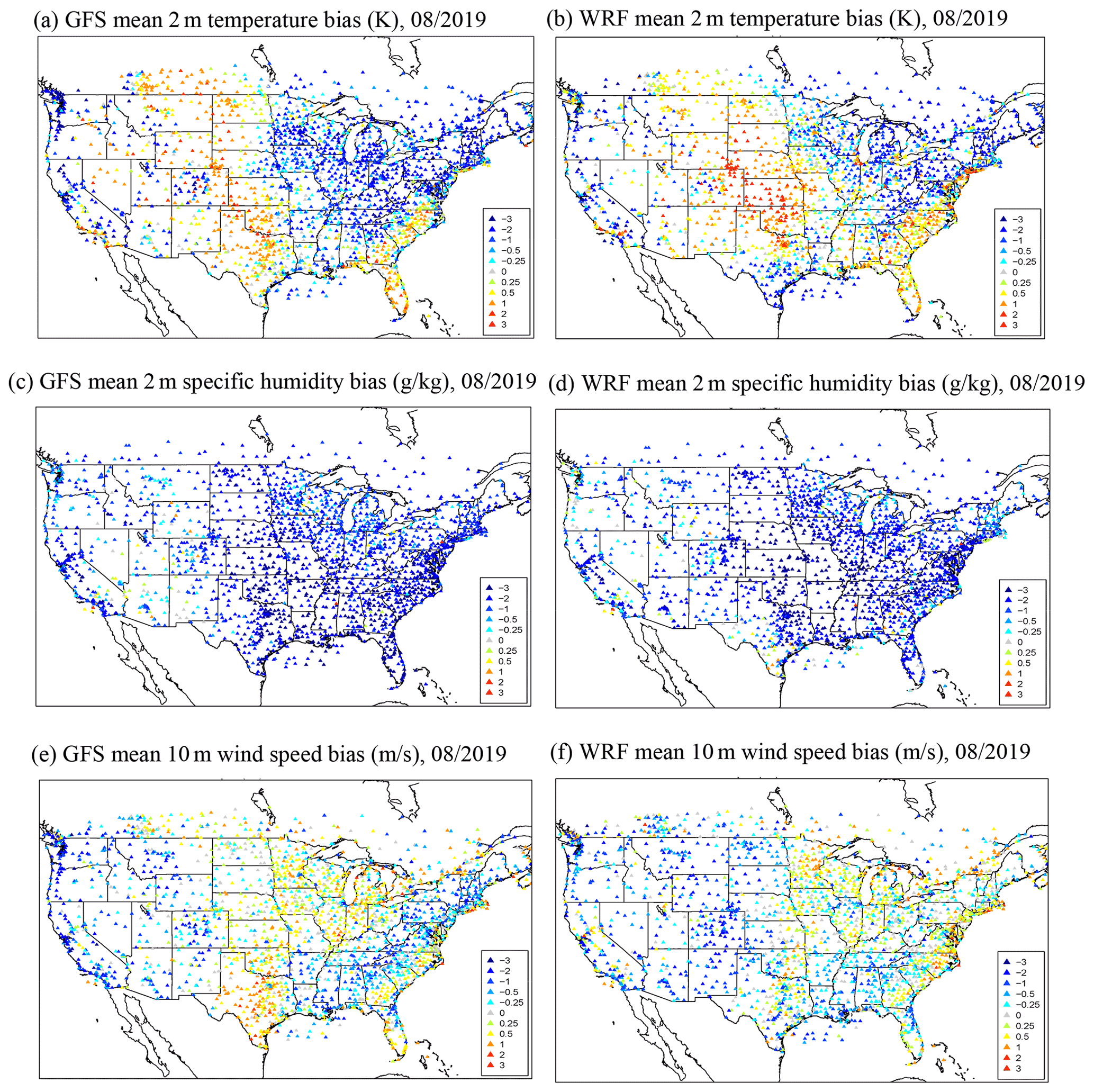
Figure 1 GFS and WRF surface meteorological biases for METAR (METeorological Aerodrome Report) stations averaged over August 2019.

Both the GFSv16 and WRF models have similar and rather significant dry biases for specific humidity (SH) predictions across the CONUS domain (Fig. 1c, d). Qian et al. (2020) investigated this common dry bias in many models and found that neglecting an irrigation contribution could cause this dry bias. Besides this issue, WRF's dry bias could also be affected by its nudging toward GFS, as GFS has widespread dry biases (Campbell et al., 2022). Their biases also have some noticeable differences over certain regions. For instance, WRF has less dry bias over southern Texas than GFS.

Both models underestimate the mean 10 m wind speeds compared with METAR stations over the western US: WRF has stronger underpredictions over the Rocky Mountains and overpredictions over northeastern US, whereas GFS has stronger underpredictions over the Appalachian Mountains and overpredictions over Texas and Oklahoma. GFSv16's operational verification (https://www.emc.ncep.noaa.gov/gmb/emc.glopara/vsdb/v16rt2/g2o/g2o_00Z/index.html, last access: 24 October 2022) also shows that it tends to underpredict the 10 m wind speed over the western US during both daytime and nighttime, but it shows overpredictions over the eastern US. Besides the difference in physical schemes (Table 1), for example, other possible reasons causing this surface wind difference could be effect of gravity-wave drag (GFSv16 includes it, but the WRF run here does not) and vertical resolutions (GFS's 127 layers versus WRF's 35 layers, although they have similar vertical layers below 1 km) (Campbell et al., 2022). Some studies (Skamarock et al., 2019) have revealed the necessity for a fine vertical resolution for atmospheric simulations, especially within the PBL, near the tropospheric top and during convective events. Insufficient vertical resolution could also cause plume dilution in chemical transport modeling (Zhuang et al., 2018). The gravity-wave drag is also known to influence the synoptic-scale dynamics of the atmospheric flow over irregularities at the Earth's surface, such as mountains and valleys, and the uneven distribution of diabatic heat sources associated with convective systems (Kim et al., 2003). Its parameterization is needed for large-scale models.

There are strong regional variabilities in the monthly mean PBL height differences between GFS and WRF during normal daytime (represented by 18:00 UTC) and nighttime (represented by 06:00 UTC) (Fig. 2). During daytime, GFS has a higher PBL height compared with WRF over the US Pacific coast, northern Rocky Mountains, and northeastern and southeastern US, but it becomes lower over the central US (e.g., Texas, Oklahoma and Kansas). At night, however, most of these regional differences between GFS and WRF are reversed. This diurnal difference is mainly driven by the different PBL schemes employed in GFS (Han and Bretherton, 2019) and WRF (i.e., YSU) and the associated other physical suites, including the land surface data. Hence, this PBL difference has strong regional variations depending on geographic differences. The GFS's PBL height has a strong diurnal variation over these regions, including the western and northeastern US, and it shows a sharp rise and collapse after sunrise and sunset, respectively (Campbell et al., 2022). These two selected times (18:00 and 06:00 UTC) are not in the transition periods for fast diurnal changes in the PBL.

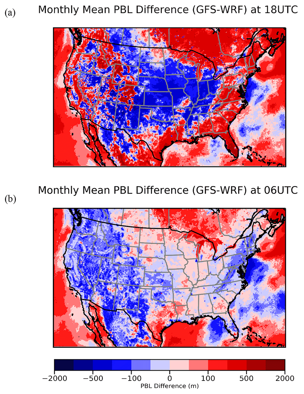
Figure 2 Monthly mean PBL height difference (GFS − WRF) for daytime (a) and nighttime (b) in August 2019.

3.2 Evaluation of regional meteorology and air quality against the AIRNow Network

The US EPA AIRNow network provides hourly observations of near-surface O₃, PM_2.5 and meteorology. Campbell et al. (2022) showed detailed verification of GFS-CMAQ with the surface AIRNow data. Here, we focus on the difference between the interpolation-based GFSv16 and WRF downscaling as well as the impacts on meteorological and chemical model performance. Figure 3 shows a comparison of these two models over two specific regions, the western US (CA, OR and WA) and the northeastern states (CT, DE, MA, MD, ME, NH, NJ, NY, PA, RI, VT and the District of Columbia) (Fig. S1 in the Supplement), where the two models have relatively large differences for some meteorological variables. GFS and WRF predict very similar 2 m temperatures over the Pacific coast states: WA, OR and CA, and both of them had a similar cool bias (around 1 K), R value and RMSE (Fig. 3a). However, these two models show significant differences with respect to the 10 m wind speed prediction over the Pacific coast (Fig. 3c), where WRF overpredicts the wind speed, especially at night and in later August. Most AIRNow stations are located near urban or suburban areas, which generally have a weaker 10 m wind speed than those at the METAR aviation weather stations near airports. For this reason, although Fig. 1e and f show that GFS and WRF underpredict the monthly mean wind speed over the METAR stations in the west, they still tend to overpredict wind (Fig. 3c) over AIRNow stations, especially for the WRF 10 m wind speed at night. Considering that the model grid cells represent 12 × 12 km² averages, the true model–observation comparisons likely fall somewhere between the urban/suburban AIRNow stations and METAR stations, depending on the land use fractions of each grid. Obviously the representation characteristics of observations could affect the verification results. Compared with AIRNow observations, GFSv16 has overall better scores for surface wind speed predictions over the western US, where the WRF's higher surface wind speed overprediction is associated with its PBL height predictions (Fig. 3e, f). During the nighttime, GFS has a lower PBL height (10 %–50 % lower than WRF) and weaker vertical mixing, which tends to bring less momentum flux from the upper layers to the surface, leading to lower nighttime wind and better agreements with the AIRNow wind speed observation.

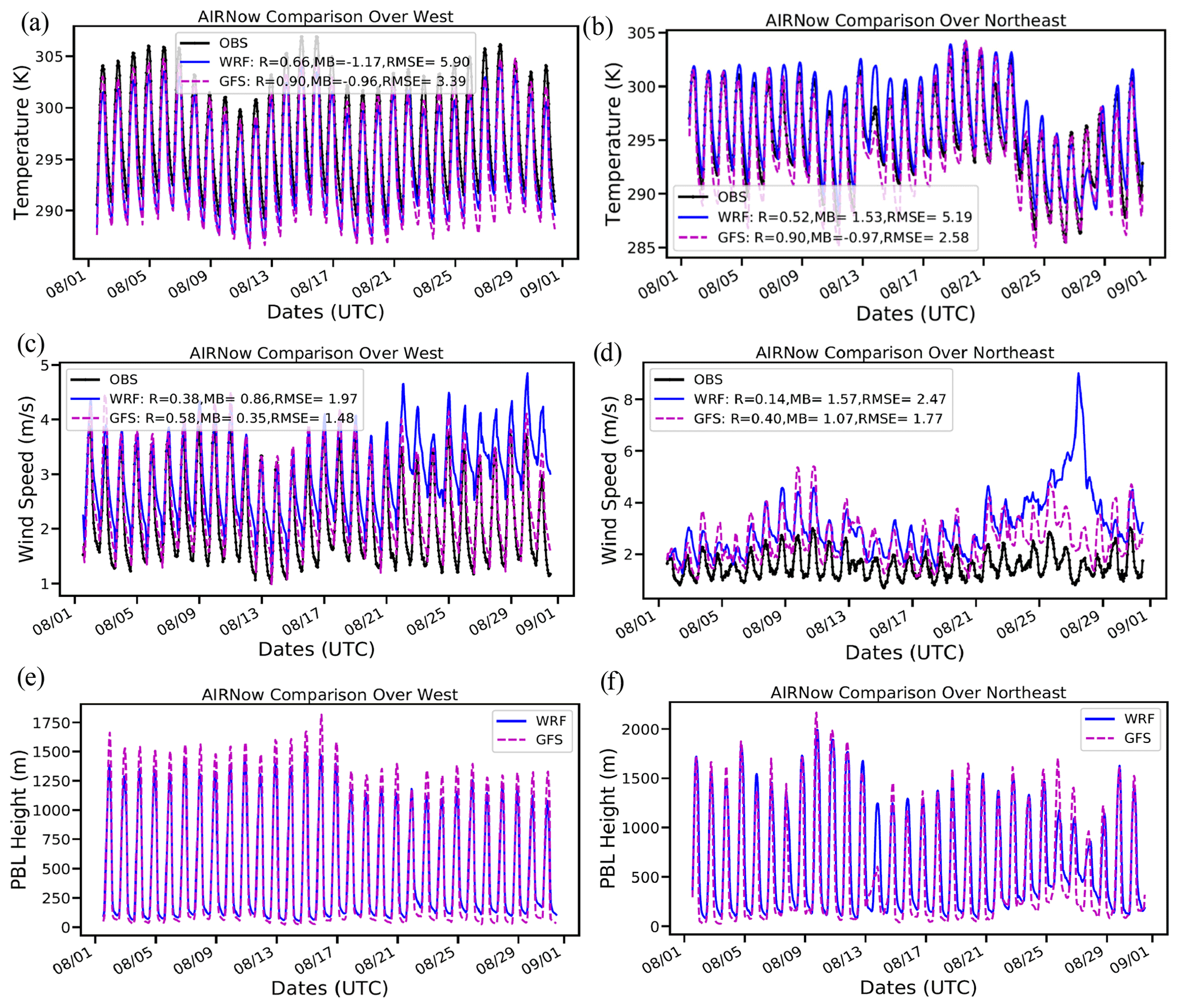
Figure 3 The WRF and GFS time series comparison for AIRNow stations over the western and northeastern US for 2 m temperature (a, b), 10 m wind speed (c, d) and PBL height (e, f).

Over the northeastern US, the mean bias (MB) of GFS temperature is about −1 K, whereas the WRF model has a slightly warm MB of about 1.53 K (Fig. 3b). However, the GFS's temperature prediction has a better correlation coefficient (R) and RMSE, implying that it better captures some events, such as the storm on 28–29 August. Both models overpredict 10 m wind speeds in the northeast, but the GFS model yields better results due to a slightly lower PBL height at night (Fig. 3f) compared with WRF, which had significant overpredictions, especially during 25–29 August (Fig. 3d) when tropical storm Erin approached this region. Especially on 28 August, when the storm was centered near the east coast of North Carolina, WRF significantly underpredicted the 2 m temperature (Fig. 3b) and overpredicted the 10 m wind speed (Fig. 3d). In the west around the same period, tropical storm Ivo appeared southwest of the Baja California Peninsula, bringing heavy rainfall to Mexico. Associated with this storm, a low-pressure system expanded over most of the western US. Differing from GFSv16, which is designed for the operational meteorological forecast, the WRF configuration used in this study is normal for driving CMAQ, but it is not tuned for storm weather prediction.

Figure 4a and b show the O₃ predictions of the two models over these two regions, and GFS-CMAQ yields predominantly lower O₃ than WRF-CMAQ, especially at night. Over the west, the lower O₃ in GFS-CMAQ is associated with their PBL height difference. First, with a certain dry-deposition velocity between the models, it is easier to deplete O₃ given the smaller volume of a shallower PBL. Second, the shallower PBL results in higher surface NO_x concentrations (not shown) and O₃ titration rates near NO_x source regions, consequently resulting in lower O₃ in these areas at night. Last, the lower PBL could decouple from the residual layer and result in weaker or no vertical O₃ exchange with the residual layer at night (Caputi et al., 2019). All of these factors contribute to the lower nighttime O₃ of GFS-CMAQ compared with WRF-CMAQ. As GFS-CMAQ already underpredicts O₃ due to combined meteorological factors, such as the temperature underprediction (Fig. 4a), the GFS-CMAQ's further O₃ reduction (possibly due to its lower PBL height at night) exacerbates its low bias. However, over the northeastern US, the similar impacts help the GFS-CMAQ yield a much better MB due to its better agreement with the observed nighttime low O₃ over this region. Over the entire CONUS domain, the situation is similar, and the GFS-CMAQ has a lower ozone MB (1.1 ppb) compared with WRF-CMAQ (4.7 ppb). Figure 5 shows that both models have similar daytime O₃ prediction over the CONUS. However, GFS-CMAQ better captures low nighttime O₃ over the eastern US than WRF-CMAQ (Fig. 5c, d).

Figure 4 Same as Fig. 3 but for O₃ (a, b) and PM_2.5 (c, d).

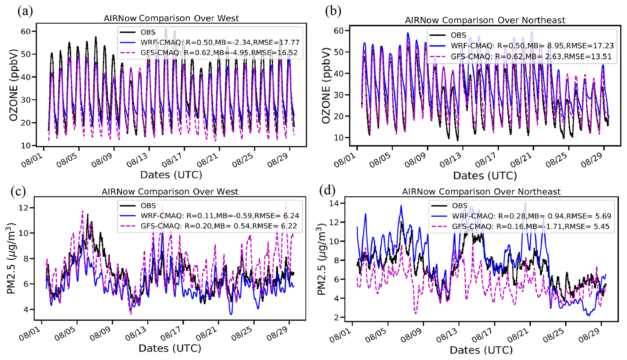
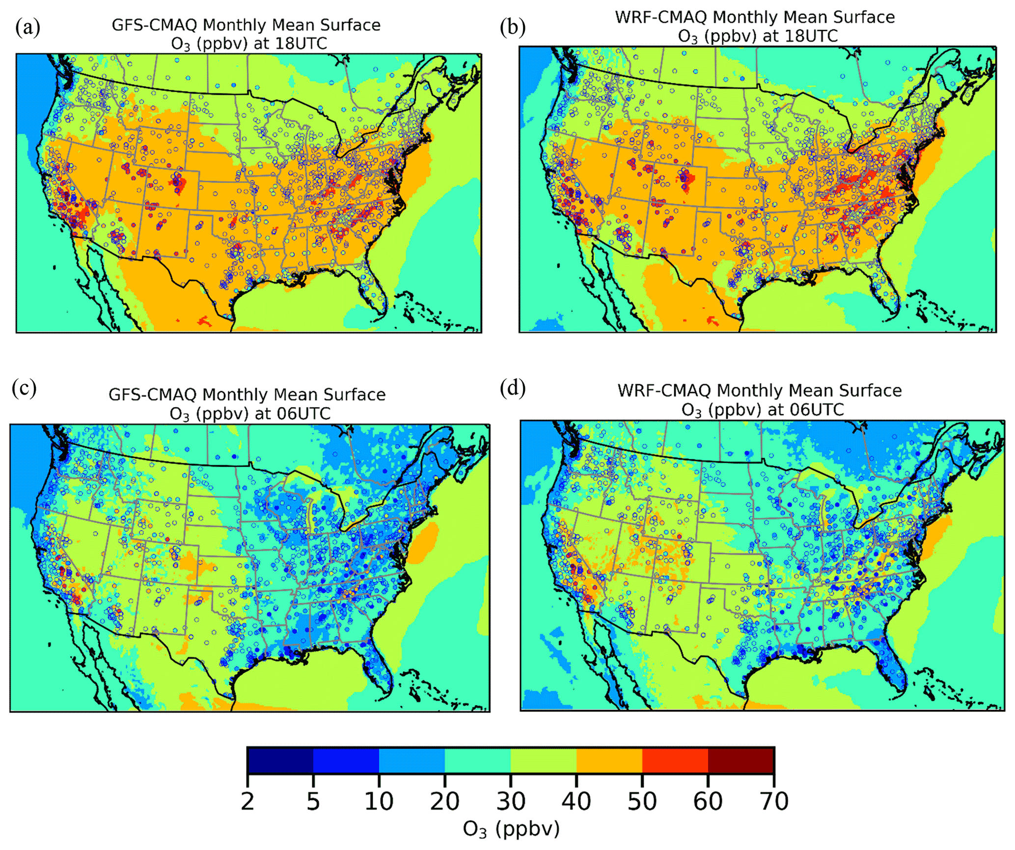
Figure 5 Monthly mean surface O₃ predictions by GFS-CMAQ (a, c) and WRF-CMAQ (b, d) for daytime (a, b) and nighttime (c, d) compared with the corresponding AIRNow observations for August 2019.

GFS-CMAQ has substantially higher PM_2.5 mean concentrations over the western US but lower mean concentrations over the northeastern US compared with WRF-CMAQ (Fig. 4c, d). These model differences are also related to their interpolated GFSv16 versus downscaled WRF meteorological drivers. Because both models use the same emissions under relatively clean background conditions in the west (i.e., prevailing westerly flow from the Pacific Ocean), the PBL and wind speed differences have significant impacts on their near-surface pollutant concentrations, especially at night. Both models show strong PM_2.5 diurnal variations (high at night and low during daytime), driven by the meteorological diurnal variation (e.g., PBL), which overcomes the emission diurnal variation (usually high during daytime and low at night). Compared with WRF-CMAQ, GFS-CMAQ has a lower nighttime PBL height and a weaker wind speed at night, which lead to weaker vertical mixing and venting, increasing the pollutant concentrations near the surface and yielding higher surface PM_2.5 over the western US (Fig. 4c). Its higher surface PM_2.5 could also result in stronger local dry deposition. In contrast to the local vertical mixing and venting effects on PM_2.5 discussed above, there are strong (and potentially counterbalancing) impacts of model PBL and horizontal wind speed differences on downstream PM_2.5 concentrations at night. WRF-CMAQ's deeper PBL and stronger wind speeds at night (Fig. 3c, d, e, f) tend to transport aerosols and their precursors more efficiently downstream via the dominant advection pathway. Figure 6 shows that these monthly mean background PM_2.5 differences appear east of the Rocky Mountains (WRF-CMAQ is about 2 µg m⁻³ higher) during both daytime and nighttime. This effect is very prominent in the northeastern region. Although both models predicted a similar PM_2.5 magnitude over the northeastern US, GFS-CMAQ yields an overall PM_2.5 underprediction, and its monthly mean PM_2.5 is 2.6 µg m⁻³ lower than the WRF-CMAQ prediction (Fig. 4d). Especially during the 1–9 August period, WRF-CMAQ had about a 4 µg m⁻³ higher surface PM_2.5 background than that of GFS-CMAQ. In this case, the WRF-CMAQ model shows better agreement with observations (Fig. 4d). It is possible that the GFS-CMAQ's nighttime PBL heights (wind speeds) are too shallow (weak) in this case, which does not allow enough transport of pollutants downstream (to the eastern USA). Overall, GFS-CMAQ and WRF-CMAQ show mixed performance with respect to PM_2.5 predictions during the August 2019 period: GFS-CMAQ has better PM_2.5 prediction over the western US, and WRF-CMAQ yields better results over the region east of the Rocky Mountains (Fig. 6).

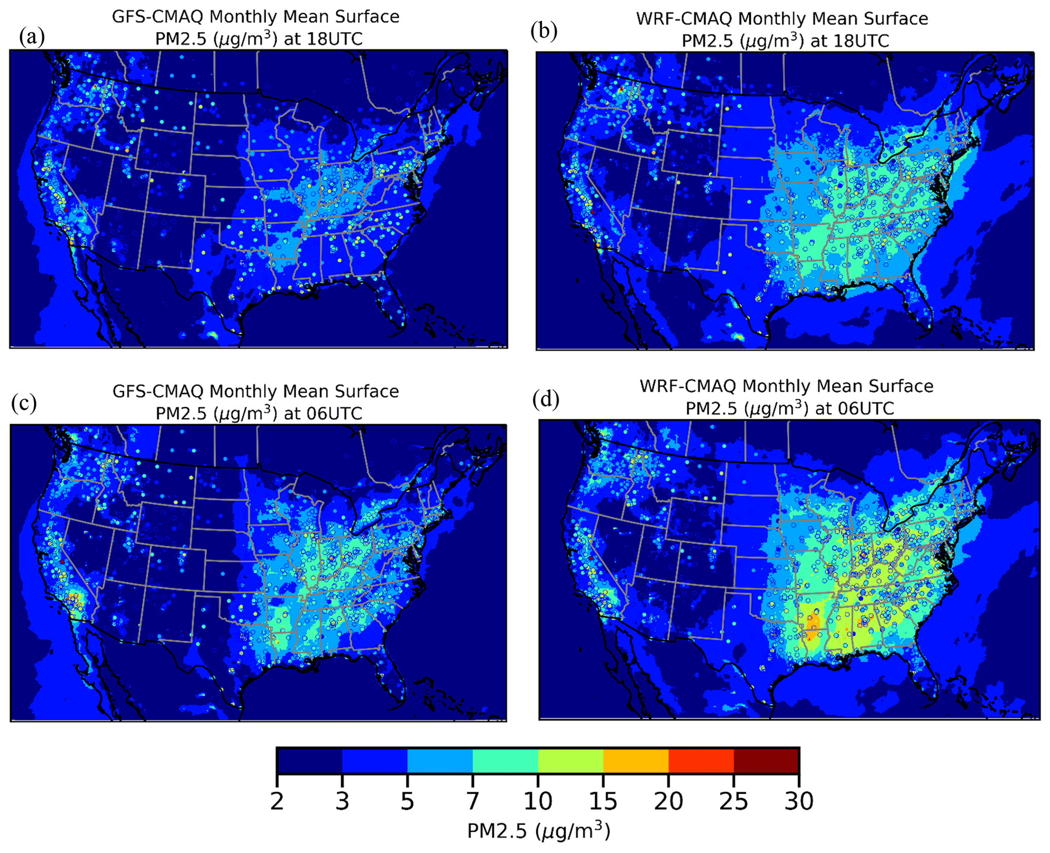
Figure 6 Same as Fig. 5 but for surface PM_2.5.

4 Model comparisons against the FIREX-AQ aircraft data

From late July to early September 2019, the joint NOAA–NASA FIREX-AQ field campaign (https://csl.noaa.gov/projects/firex-aq/, last access: 24 October 2022) employed a suite of satellites, aircraft, vehicles and ground site platforms aimed at observing, analyzing and characterizing air pollutants emitted from wildfire sources over the CONUS (Ye et al., 2021). The FIREX-AQ airborne measurements provide a 3D dataset from various meteorological, gas and aerosol instruments that can be used to verify the GFS-CMAQ and WRF-CMAQ model performance while also elucidating reasons for any model differences. Here, the focus of the FIREX-AQ model comparison and verification is against observations taken primarily from the NASA DC-8 aircraft, which include meteorological variables, gaseous and aerosol concentrations, and aerosol optical properties merged at a 1 min temporal resolution. The model data are spatiotemporally interpolated to the flight paths for comparison. The majority of the FIREX-AQ flights were over the western US, and they sampled within environments that both were and were not (see Sect. 4.1) influenced by wildfire emissions (https://daac.ornl.gov/MASTER/guides/MASTER_FIREX_AQ_JulySept_2019.html, last access: 24 October 2022). During a cluster of major wildfire events (see Sect. 4.2), the DC-8 sampled both near-source and aged smoke plumes between 2 and 8 August 2019 (i.e., the Williams Flats, Snow Creek and Horsefly fires) across the states of ID, WA and MT.

4.1 Comparison of the 22 July non-wildfire event over the central California Valley

On 22 July, the DC-8 aircraft flew from California to Boise, ID, while maintaining a relatively low altitude (< 1 km a.s.l., above sea level) over the California Central Valley (Fig. 7). This flight was not impacted by any major wildfire event and was mainly controlled by anthropogenic emissions and local meteorological conditions. Figure 7 shows that the GFSv16 and WRF models had similar meteorological temperature and humidity predictions and that both models have dry and warm biases over the Central Valley at lower altitudes (Fig. 7d, e) (Qian et al., 2022). GFS's horizontal wind speeds tend to have a stronger variability than WRF (Fig. 7b), especially in high altitudes. With respect to wind direction, WRF shows a better prediction than GFS around 20:00 and 24:00 UTC (Fig. 7c).

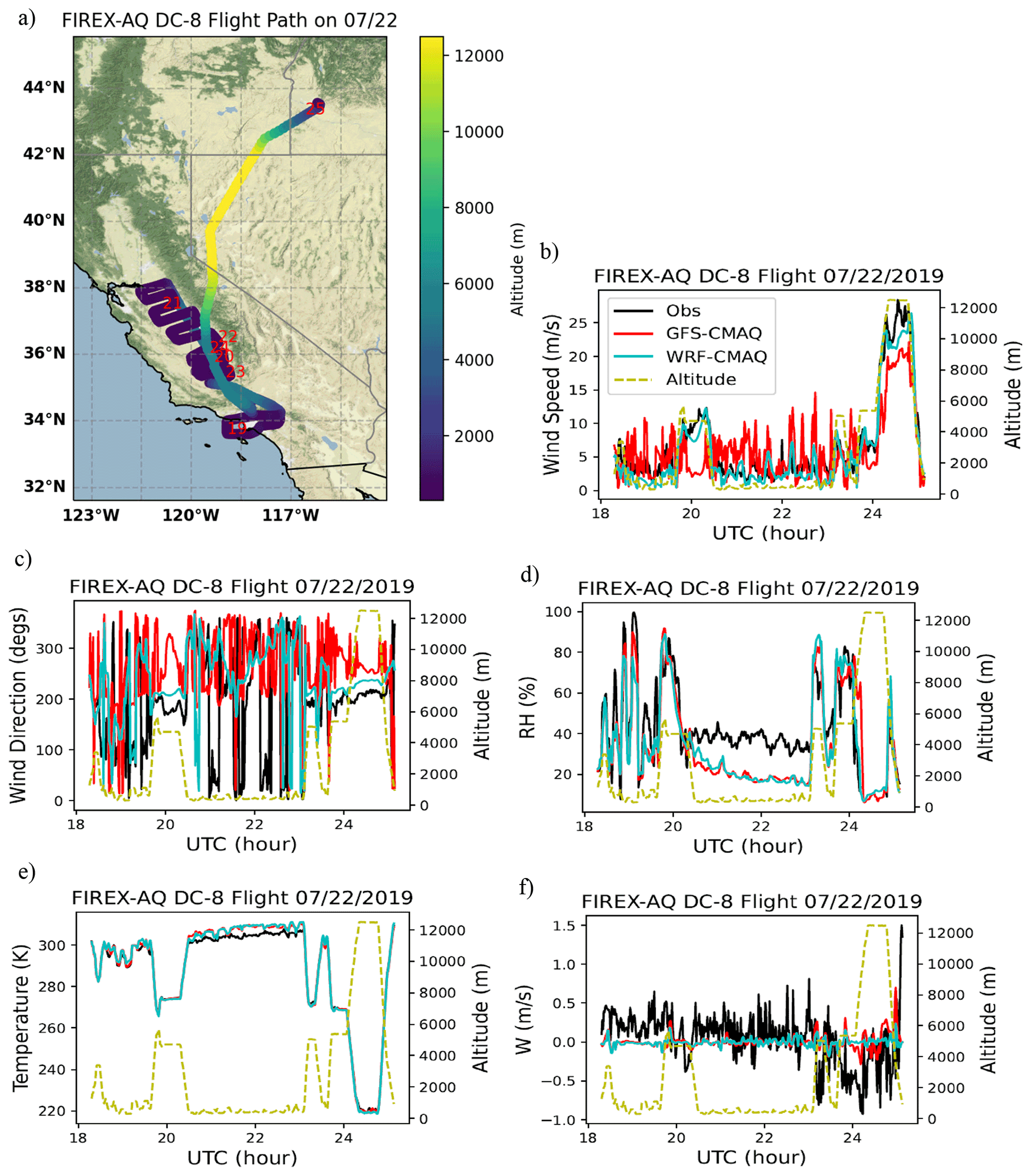
Figure 7 Modeled meteorological variables compared with observations for the DC-8 flight on 22 July 2019 (b–f). Panel (a) shows the flight path color-coded by altitude above sea level with the UTC time given in red text. Base map credits: © OpenStreetMap contributors 2022. Distributed under the Open Data Commons Open Database License (ODbL) v1.0.

Both GFS-CMAQ and WRF-CMAQ underestimate the vertical wind (W) variability by at least 1 order of magnitude, and WRF-CMAQ has weaker W variability than that of GFS-CMAQ, especially at high altitudes (Fig. 7f). The model vertical velocities are not directly from the GFS nor the WRF model; rather, they are re-diagnosed in CMAQ to conserve mass (Otte and Pleim, 2010) and, thus, represent the whole layer's vertical movement across the 12 km × 12 km grid cell. With its flight speed of around 80 to 240 m s⁻¹, the DC-8 aircraft's 1 min average sampling frequency results in an approximate 4.8 to 14 km horizontal scale, respectively, which is comparable with the 12 km CMAQ model resolution. The aircraft observations, however, include turbulence effects during its 1 min averages, which may not be temporally resolved by the models at this resolution. Thus, both the GFS-CMAQ and WRF-CMAQ vertical velocities are much lower and have almost no correlation with the aircraft observations.

Although both GFS-CMAQ and WRF-CMAQ have reasonable comparisons for most meteorological variables, including the horizontal winds, it continues to be a challenge to compare them with the observed vertical velocities. Thus to further elucidate the model–observation differences in vertical motion, Fig. 8 shows a curtain plot of vertical velocities along the flight path from the two models. As WRF-CMAQ remains on a native grid, its wind fields tend to be more balanced and have lower variability compared with the GFS-CMAQ wind fields. The stronger variability in W for GFS-CMAQ could be caused by GFS's non-hydrostatic dynamics or CMAQ's effort to counteract mass-inconsistency effects from the interpolated horizontal wind fields (Byun, 1999b). Our comparison shows that the first factor should be the major one (Fig. S2) for this event, as the GFS-CMAQ-diagnosed W is very similar to that from the original GFSv16 around 1 km a.g.l. (above ground level). As the original GFSv16 also has similar stronger vertical velocities compared with the original WRF, the W difference between GFS-CMAQ and WRF-CMAQ is unlikely to be due to interpolation error in the horizontal winds.

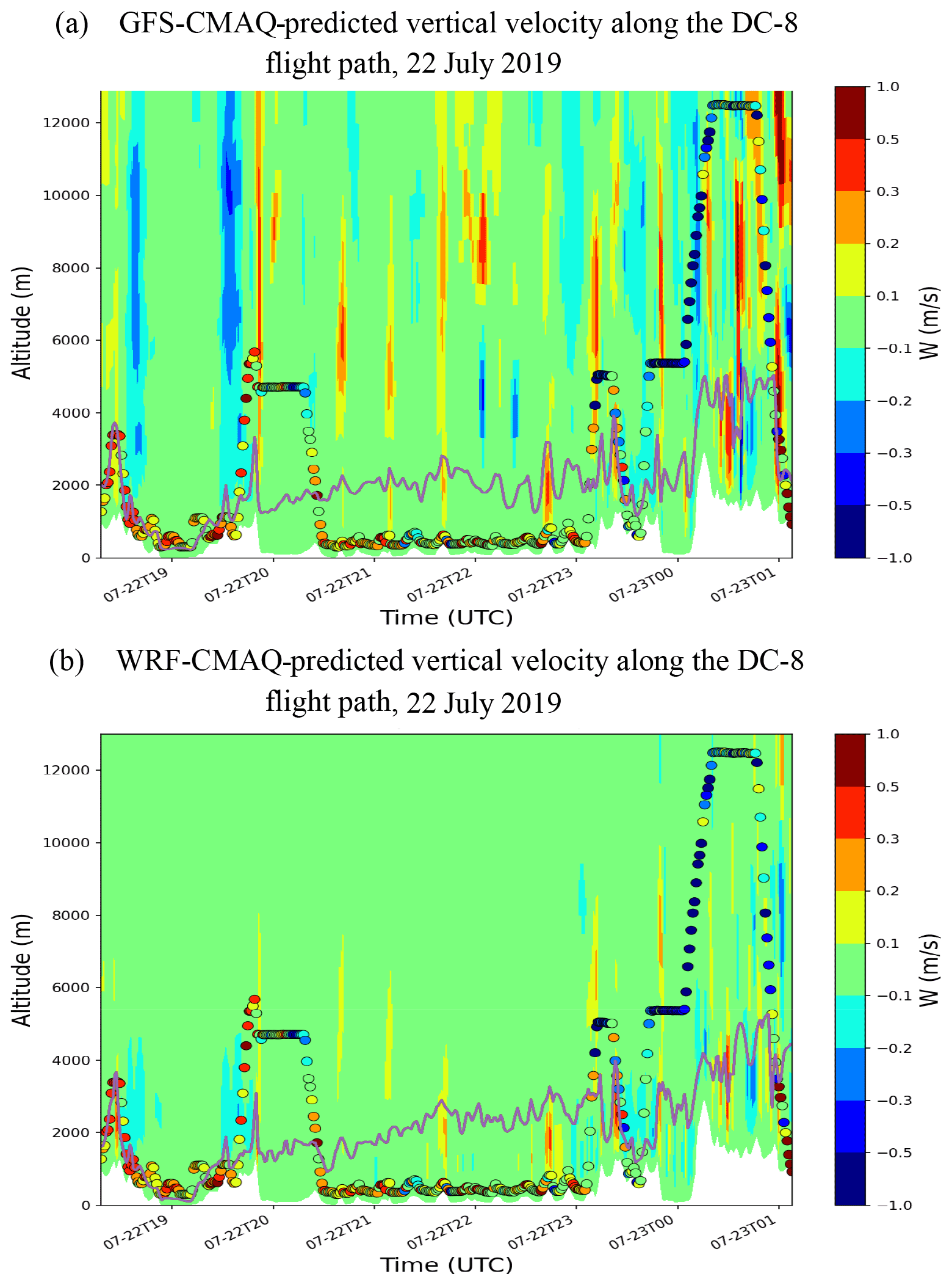
Figure 8 Curtain plots of the vertical velocity (W) predicted by GFS-CMAQ (a) and WRF-CMAQ (b) along the DC-8 flight on 22 July 2019. The colored dots show the DC-8-measured vertical velocities, and the solid lines show the predicted PBL heights of these two models.

GFS-CMAQ and WRF-CMAQ yield similar results overall for specific chemical species during this DC-8 flight (Fig. 9). Both models underestimate CO, O₃ and ethane (C₂H₆) concentrations over the lower altitudes in the California Central Valley. Over the same flight segment, they have better NO_x (NO + NO₂) and ethene (C₂H₄) predictions, implying that the emissions of these two species have better accuracy than those of CO and C₂H₆. Figure 9f shows that the two models also underestimate NO_z (NO_y–NO_x), or the oxidized nitrogen species besides NO_x, indicating that photochemical O₃ production may also be underestimated. NO_z is a good indicator of the O₃ photochemical formation (Sillman et al., 1997), where the ${\mathrm{O}}_{\mathrm{3}}/{\mathrm{NO}}_z$ ratio represents the O₃ photochemical efficiency per NO_x oxidation product. Thus, NO_z and O₃ are typically highly correlated over regions with active photochemical production. Our later analysis shows that the models tend to underestimate certain hydrocarbons, such as C₂H₆, which is likely linked to O₃ and NO_z underestimations, as the hydrocarbons are photochemical precursors of O₃ and NO_z.

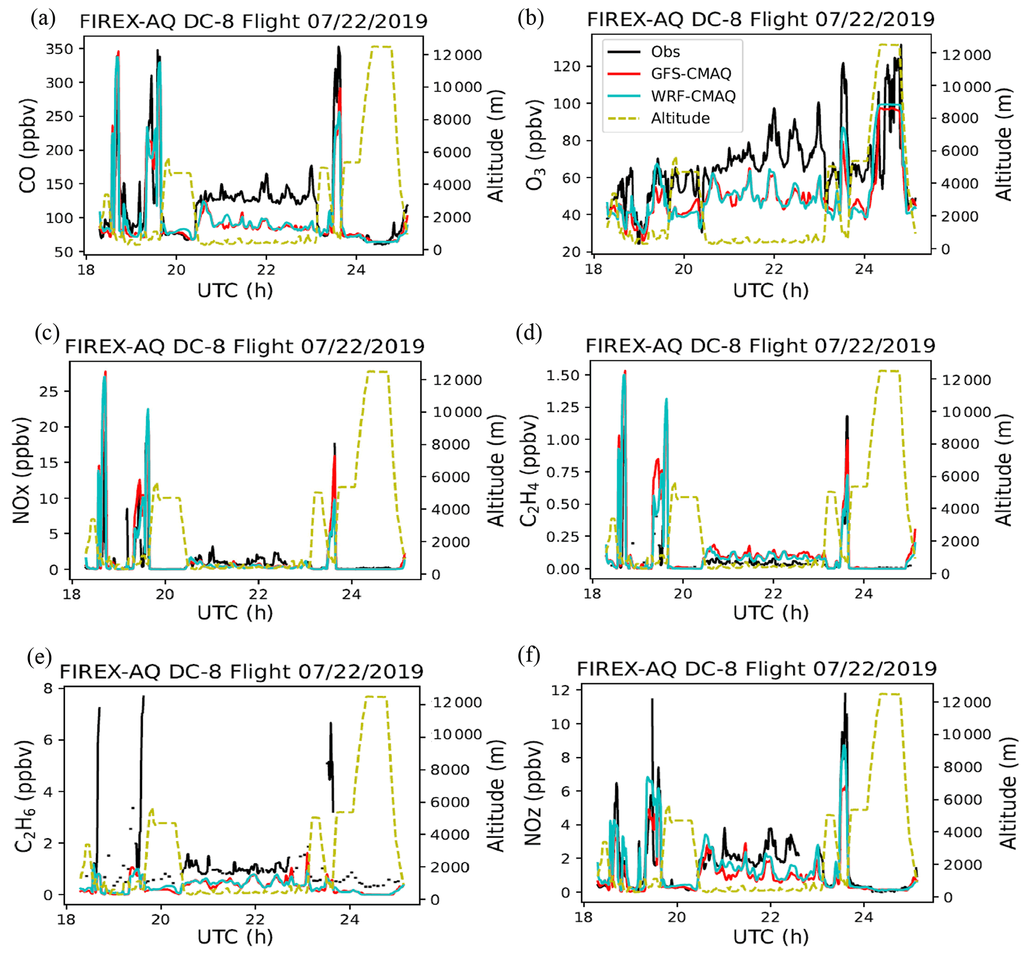
Figure 9 Model-predicted chemical concentrations compared with observations along with the DC-8 flight on 22 July 2019.

The two models show slight differences in peak values of CO, C₂H₄ and NO_x around 23:30 UTC: the GFS-CMAQ-predicted concentrations are slightly higher and closer to observations (Fig. 9). These differences are due to their PBL predictions (both from the corresponding meteorological model outputs): GFS-CMAQ has a lower PBL height and weaker emission vertical dilution compared with WRF-CMAQ (Fig. 8). However, GFS-CMAQ tends to underpredict O₃ more (Fig. 9b) due to its higher NO_x titration. This implies that the effects of the transport and nonlocal transformation of O₃ could be stronger than that of local precursor emissions. WRF-CMAQ has higher NO_z (Fig. 9f) but lower NO_x compared with GFS-CMAQ due to the time lag of O₃ and NO_z photochemical formation. Consequently, the peak O₃ values may not be well correlated with the emitted precursors, such as NO_x and VOCs. Furthermore, the modeled peak C₂H₆ and C₂H₄ concentrations do not occur at the same time around 23:30 UTC, whereas observations indicate that these two species should be highly correlated in this region. This model mismatch implies that the VOC speciation factors for a certain area or emission sector need to be improved over Southern California.

4.2 Comparison of the 6 August wildfire events over the northwestern US

On 6 August, the DC-8 observed a cluster of three wildfires: the Williams Flats fire (47.98^∘ N, 118.624^∘ W; 80 km to the northwest of Spokane, WA), the Snow Creek fire (47.703^∘ N, 113.4^∘ W; 32 km northeast of Condon, MT) and the Horsefly fire (46.963^∘ N, 112.441^∘ W; 24 km east of Lincoln, MT). Figure 10a shows the flight path on that date: the DC-8 aircraft departed from Boise, ID; flew over the Williams Flats fire region; flew to Montana to sample the Snow Creek and Horsefly fires (i.e., Montana fires); and finally returned to the Boise base. The aircraft flew below 8 km for most flight segments near the fire plumes. Figure S3 shows the corresponding GOES-16 satellite true-color image, where these 6 August fires and the associated smoke plumes are visible and can be distinguished from the cloud bands to the south that move northward later that day (Fig. S3). The Williams Flats fire was ignited by lightning and was the largest fire event sampled during the FIREX-AQ campaign, burning from about 2–8 August 2019.

Figure 10 The DC-8 flight path (a) as well as model–observation comparisons for O₃ (b), CO (c), NO₂ (d), submicron organic aerosol (OA) (e) and the aerosol optical extinction coefficient (AOE) at a wavelength of 550 nm (f) on 6 August 2019. Base map credits: © OpenStreetMap contributors 2022. Distributed under the Open Data Commons Open Database License (ODbL) v1.0.

Both models significantly underpredicted CO (Fig. 10c), submicron (aerosol diameter < 1 µm) organic aerosol (OA) (Fig. 10e) and the aerosol optical extinction coefficient (AOE) (Fig. 10f), suggesting an issue with the GBBEPx gas and aerosol emissions. The models performed well for NO₂ during the Williams Flats and Montana fires below 6 km a.s.l., but there were prominent underestimations for the high-altitude flight segments (Fig. 10d). However, as the NO₂ instrument (the NOAA NO_yO₃ four-channel chemiluminescence instrument) had an NO₂ detection limit of around 0.01 ppb (https://airbornescience.nasa.gov/sites/default/files/documents/NOAA NOyO3_SEAC4RS.pdf, last access: 24 October 2022), the models might not truly underestimate NO₂ for these flight segments with extremely low NO₂. WRF-CMAQ predicted higher O₃ values than the GFS-CMAQ, which generally agreed better with observations for the Williams Flats fire (Fig. 10b). However, for the Montana fires (∼ 23:00–24:00 UTC), WRF-CMAQ has higher O₃ biases, and GFS-CMAQ yields better results. The difference in O₃ is largely driven by the regional background concentration difference between the two models: WRF-CMAQ tends to have higher domain-wide O₃ concentrations than GFS-CMAQ due to the meteorological effects discussed in Sect. 3, even though they used the same lateral boundary conditions.

Figure S4 shows the spatial overlay comparison of vertically averaged GFS-CMAQ predictions at 21:00 UTC and the DC-8 flight observations for the altitude of 1–3 km a.g.l. on 6 August 2019. The peak NO₂ observation around 48^∘ N, 118.5^∘ W indicates the general location of the Williams Flats fire. The GBBEPx emissions and GFS-CMAQ prediction showed shifted peak-value locations driven by the westerly modeled winds. For this flight, the GBBEPx had stronger NO_x fire emissions over two Montana locations than that over Williams Flats. The model overpredicts the column-averaged NO₂ concentrations, especially over the Montana fires, which can not be reflected by the point-by-point NO₂ comparison result in Fig. 10d. For this flight, the mean GFS-CMAQ NO₂ along the flight path for 1–3 km a.g.l. is about 0.125 ppbv compared with the observed mean NO₂ of 0.169 ppbv, and the model indeed showed an NO₂ underprediction along the flight path. However, in this case, the flight path did not encounter the locations with modeled peak NO₂ values, as the model misplaced the plumes, especially over the Montana fires, leading to this inconsistency. With respect to the O₃ comparison (Fig. S4b), this inconsistency could also exist, although it may not be as significant as the inconsistency for the high-gradient NO₂ concentrations. In the GFS-CMAQ prediction, the high O₃ concentrations are almost co-located with high NO₂ concentrations (Fig. S4b), but the observations did not show this feature. Instead, some high-O₃ flight segments had relatively low NO₂ concentrations, such as those circled in the black rectangle in Fig. S4b. The observed NO_x titration was not able to be produced by the 12 km models. Wang et al. (2021) used a 100 m horizontal resolution large-eddy simulation and demonstrated the capability of using such techniques to capture some high-resolution features of fire plumes and the associated chemical behavior. While such high-resolution techniques are not currently feasible for the operational NAQFC, they demonstrate the limitation of using regional-scale (12 km × 12 km) models to capture such fine-scale features of the fire plume.

GFS-CMAQ has higher wildfire-related CO, NO₂, OA and AOE values that are closer to observations than WRF-CMAQ for the Montana fires between 23:00 and 24:00 UTC at flight altitudes of ∼ 4–5 km (Fig. 10c, d, e, f). As these two models use the same GBBEPx emissions and wildfire plume rise algorithm (Briggs, 1965), the differences should be due to other reasons. To help explain these model differences, Fig. 11a and b show the aerosol backscatter coefficients (ABCs) retrieved by the differential absorption high-spectral-resolution lidar (DIAL-HSRL) aboard the DC-8 aircraft without and with cloud screening, respectively. It shows that the major fire plumes of the William Flats fire were below 4 km (∼ 19:00–22:00 UTC), but the Montana fires (∼ 23:00–24:00 UTC) extended from the surface up to 6 km, with some detached plumes reaching 10 km. The model-predicted AOEs have an overall similar pattern, with major plumes below 4 km for the Williams Flats fire (Fig. 11c, d). Over the Montana fires, the GFS-CMAQ predicts a slightly higher PBL height, thereby allowing the fire plume to reach a higher height near the DC-8 cruising altitude. In contrast, the WRF-CMAQ wildfire plumes are slightly lower than the aircraft flight path around 23:00–24:00 UTC, which leads to underpredictions of the fire-emitted species (Fig. 11d).

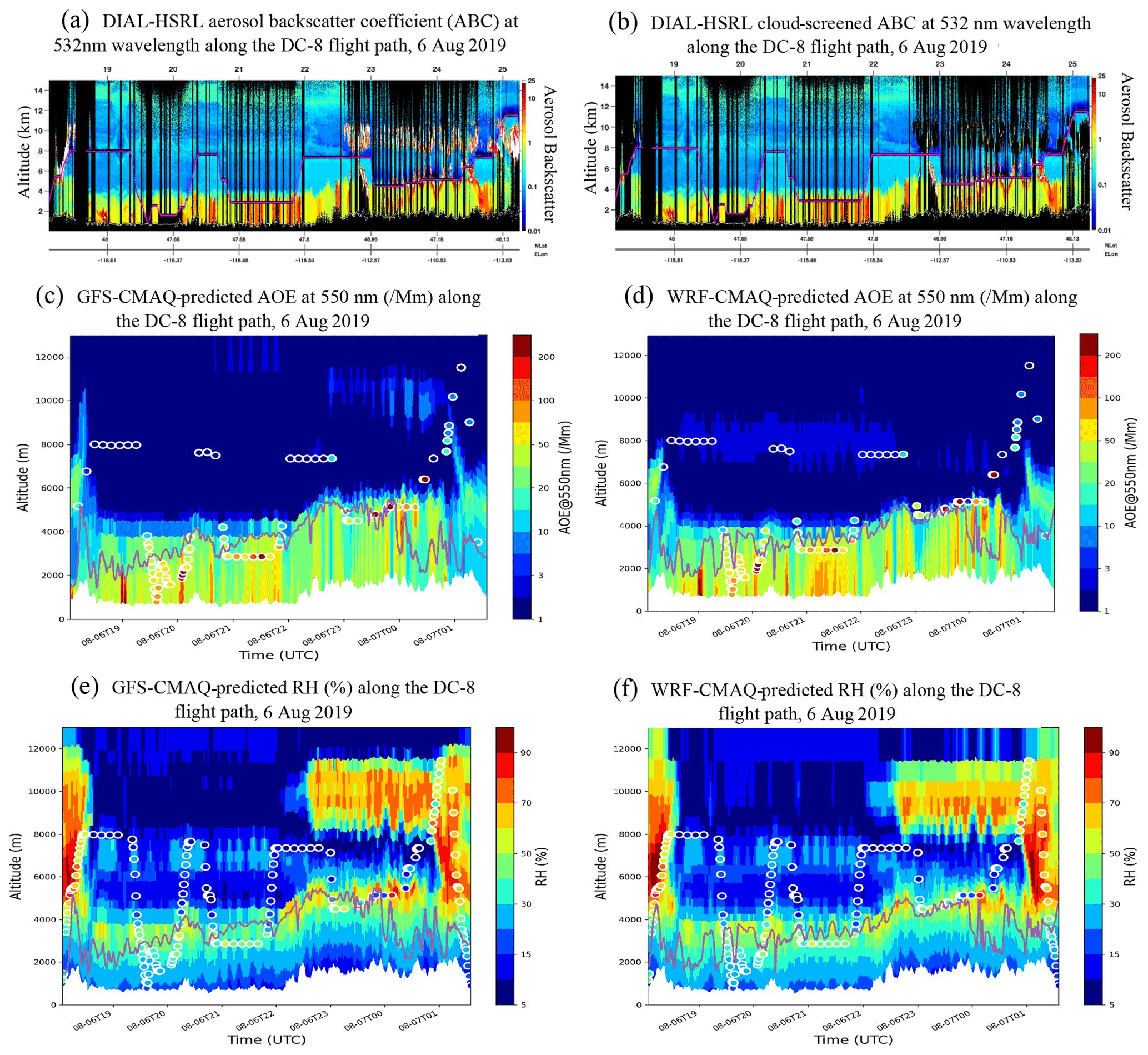
Figure 11 The differential absorption high-spectral-resolution lidar (DIAL-HSRL) retrieved aerosol backscatter coefficients (ABCs) at a 532 nm wavelength in steradians per kilometer (a), the cloud-screened ABCs (b), curtain plots of the AOEs (b, c), and relative humidity (RH) predicted by (d) GFS-CMAQ and (e) WRF-CMAQ along the DC-8 flight on 6 August 2019. The colored dots show the corresponding measured values, and the solid lines show the predicted PBL heights of these two models.

An interesting feature in the DIAL observations is the detached plume from 8 to 10 km altitude (Fig. 11a): some cirrus clouds existed in this region, and the DIAL retrieval could not distinguish whether they were pure clouds or clouds mixed with elevated aerosols above 8 km. The cloud-screened image (Fig. 11b) mainly showed the enhanced aerosols below 7 km and some scattered signals near the high cloud edges. Cloud mixing with aerosols was usual for fire-induced clouds, or pyrocumulonimbus (Peterson et al., 2021). Although, in this event, the middle-sized fires did not show evidence of inducing high-altitude clouds, the indicators of mixed clouds and aerosols at high altitudes still existed: both OA measured in situ (Fig. 10e) and the AOE (Figs. 10f; 11c, d) showed the enhanced aerosols around 01:00 UTC of the next day above 8 km. This elevated plume was generally captured by the GFS-CMAQ simulation, although its strength was underestimated (Fig. 11c); however, this feature was completely missed in WRF-CMAQ (Fig. 11d). Considering the altitude range of the detached plume, the major model disparities are likely due to model convection differences in the free troposphere. To further investigate this impact, Fig. 11e and f show curtain plots of relative humidity (RH) predicted by the two models. GFS-CMAQ yields higher RH at such altitudes (10 km) compared with WRF-CMAQ around 23:00–24:00 UTC, indicating that GFS-CMAQ has a stronger convection. The CMAQ model uses input meteorology to diagnose convection activity and drive its Asymmetric Convective Model, version 2 (ACM2) convection scheme. This convective activity is apparent in GOES-16 satellite images (Fig. S3), as more fractional clouds appeared ahead of the northward-moving frontal band. Both the GFSv16 and WRF models used here do not consider the fire heat feedback effect; thus, their predicted convection and clouds are only driven by the synoptic weather conditions. If such synoptic-to-mesoscale weather models consider wildfire heat feedback effects, their predictions may result in stronger convection and help correct their underpredictions of PBL heights.

4.3 Statistical results of model performance for FIREX-AQ

4.3.1 Meteorological statistics

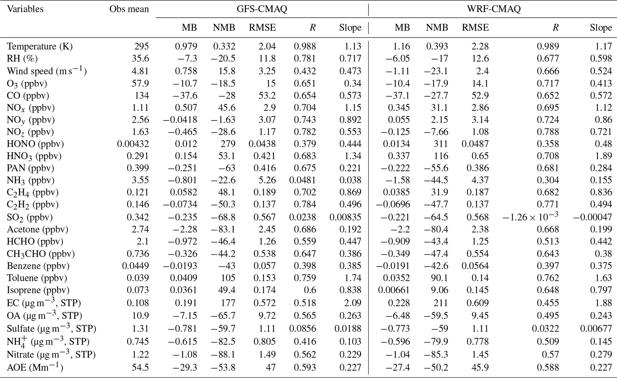
During the FIREX-AQ field campaign, the DC-8 aircraft performed more than 20 flights over the CONUS with detailed observations of various chemical compounds. Tables 2 and 3 show the statistical results of the mean bias (MB), normalized mean bias (NMB), root-mean-square error (RMSE), correlation coefficient (R) and linear regression/slopes for the two models' performance over the western US (west of 110^∘ W) only at low altitudes (< 3 km a.s.l.) for both non-fire and fire flight segments. The FIREX-AQ aircraft data included the smoke flag to mark the sampling times associated with fire plumes, identified by CO and aerosol enhancement over background levels in downwind areas of specific fires. This smoke flag is used to distinguish the flight segments with and without fire influences. Most of these flights departed from Boise, ID, except for the 22 July flight that flew from California to Idaho. As a result, they mainly flew over Idaho and its surrounding regions. The GFS tends to have a slightly higher wind speed with a positive MB, whereas WRF has a small negative wind speed bias. Most of the DC-8 flights are during the daytime, and the GFS has a higher daytime wind speed than WRF at low altitudes. The GFS and WRF have very similar temperature predictions. For the RH, the GFS predictions are slightly dryer than those of WRF, especially for non-fire events. The meteorological models do not consider wildfire heat effects and, thus, may have (in part) led to slightly warm MBs for the non-fire events (Table 2) and slightly cool MBs for the fire events (Table 3). Because both the GFSv16 and WRF models have similar MB shifts from an average temperature overprediction (Table 2; non-fire events) to an underprediction (Table 3; wildfire events), we can estimate that the fire effects cause roughly a 1–2 K temperature enhancement to the background along the DC-8 flight paths below 3 km. This estimate assumes that the model temperature biases are generally representative of the western US (west of 110^∘ W) and are independent of the averaged flight segments that have different locations and periods in Tables 2 and 3. Correspondingly, the air masses are dryer in the sampled wildfire plumes, as shown by the large reduction in the RH underpredictions (i.e., negative MBs) from Tables 2 to 3.

Table 2 Statistics of the two models compared to the observations for DC-8 flight segments without fire influences below 3 km a.s.l. over the region west of −100^∘ W. All aerosols have a diameter of less than 1 µm. The normalized mean bias (NMB) is given as a percentage.

STP denotes standard temperature and pressure.

Table 3 Table 3 is the same as Table 2 except that it displays the wildfire-affected flight segments.

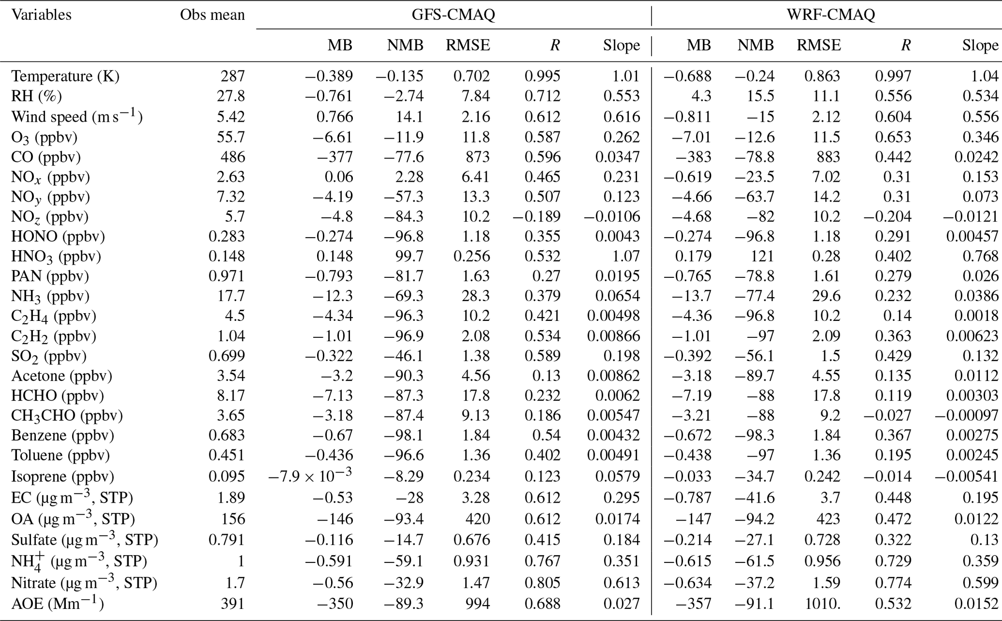
STP denotes standard temperature and pressure.

4.3.2 Chemical statistics for flight segments without fire influences

For most chemical species, the two models also have similar performance, indicating that the emissions and chemistry are major driving forces. For flight segments not encountering fire plumes, both models overpredict NO_x, HNO₃, toluene, elemental carbon (EC) and ammonium (NH${}_{\mathrm{4}}^{+}$), but they underestimate peroxyacetyl nitrate (PAN), benzene, C₂H₂, SO₂, and submicron sulfate and OAs (Table 2). The SO₂ and submicron sulfate underprediction may be impacted by underestimated NEIC2016v1 SO₂ emissions over the western US. As point sources, including power plant emissions, are the SO₂ sources, this comparison implies that the point sources for 2019 events have large uncertainties.

Although the models agree well with NO_y observations, they disproportionately underestimate NO_z (non-NO_x reactive nitrogen species, or NO_y–NO_x), as shown by the regression slopes and MBs. The NO_x and NO_y observations have different missing data, and NO_z is calculated when both NO_x and NO_y observations are available at certain sampling times. Due to the different sample number issues, their observed averages may not exactly match well (averaged NO_x + NO_z ≠ NO_y in observations), although their corresponding modeled relationship are well balanced. Gaseous NO_z species can be split into inorganic NO_z (e.g., HNO₃, HONO, HNO₄, NO₃, ClNO₃ and N₂O₅) and organic NO_z (e.g., PAN, methyl peroxyl acetyl nitrate – MPAN and the other organic nitrate – RNO₃). The precursors of organic NO_z include hydrocarbons. One of the important organic NO_z species is PAN, and both models underestimate PAN for the flight segments without fire influences (Table 2). The carbonyl precursors of PAN include acetaldehyde (CH₃CHO) (44 % of the global source), methylglyoxal (30 %), acetone (7 %), and a suite of other isoprene and terpene oxidation products (19 %) (Fischer et al., 2014). CH₃CHO and acetone are also underestimated (Table 2), which helps to explain the underestimation of PAN. For the oxidized hydrocarbons, like aldehydes (e.g., HCHO and CH₃CHO), their main atmospheric sources come from the oxidation of highly reactive VOCs, including alkanes, alkenes and aromatics, instead of direct emissions (Parrish et al., 2012). Therefore, the underestimations of HCHO and CH₃CHO are associated with the underestimations of their precursor hydrocarbons, including anthropogenic and biogenic VOCs. Our internal comparison with some limited surface VOC observations indicated that BEIS tends to underpredict biogenic emissions over the western US (e.g., isoprene in Table 2). In this comparison, most anthropogenic hydrocarbons are disproportionately underestimated, except toluene, implying a VOC speciation issue in the NEIC2016v1 anthropogenic emissions (Table 2). A previous study discovered that a model overprediction in toluene was also related to the toluene speciation in the NEIC emission inventory (Lu et al., 2020). In this comparison, both models tend to underpredict organic NO_z, which is likely caused by the underestimation of certain VOCs.

Submicron ammonium (NH${}_{\mathrm{4}}^{+}$) and nitrate ion (NO${}_{\mathrm{3}}^{+}$) are also underestimated by both models during non-fire events (Table 2), suggesting there are NH₃ underestimates due to either insufficient NH₃ emissions or exaggerated NH₃ removal processes. There are, however, overpredictions in the intermediate species nitric acid (HNO₃), indicating a shift in the gas–aerosol equilibrium partitioning of the nitrate ion. This implies that HNO₃ accumulates in the atmosphere because the modeled NO_x and inorganic NO_z (such as NO₃) pathways toward the nitrate ion and organic NO_z are reduced due to underestimations of their other precursors (NH₃ and VOCs).

There are underestimations in the VOC and CO concentrations that contribute to the O₃ underestimation during non-fire flight segments (Table 2). These non-fire comparisons also highlight that both models have similar biases due to similar meteorology (Sect. 4.3.1) as well as the use of the same anthropogenic emissions (NEIC2016v1), BEIS biogenic emissions and chemical models/mechanisms (i.e., CMAQv5.3.1). The differences in the two models' bias, error and correlation/slope are much smaller than their individual magnitudes. As discussed above, VOC speciation in the emission inventory could be one issue, as the model tends to overpredict C₂H₄ but underestimate species such as C₂H₂ and C₂H₆. Some common biases over certain regions could be related to certain common issues. For instance, some power plants that were supposed to shut down in the original NEIC2016 inventory might still have been emitting pollutants during the flight observations, leading to the disagreement with respect to SO₂.

4.3.3 Chemical statistics for flight segments with fire influences

The WRF-CMAQ and GFS-CMAQ models significantly underestimate CO, VOC, HONO and OA for fire-influenced flight segments at low altitudes (< 3 km) over the western US (Table 3). In conjunction with underestimated GBBEPx emissions during these wildfire events, other possible causes for the average statistical underprediction are the CMAQ model's 12 km horizontal resolution and the flight sampling coverage. Most of the fires that are averaged in the statistics, such as the Horsefly (5.5 km² burning area) and Snow Creek fires (7.3 km² burning area), are at a much finer scale than the model grid. Only the largest Williams Flats fire, with a total burning area of 180 km² (Ye et al., 2021), had a comparable horizontal scale to the model resolution.

The DC-8 aircraft had many flight segments near wildfire sources during the fire events in Table 3; thus, dilution of the emissions due to the relatively coarse model resolution may lead to underestimations in the predicted slope for most wildfire-emitted pollutants, such as CO and OA (Table 3). The O₃ concentrations are also underestimated; however, the O₃ underpredictions are reduced from the non-fire (Table 2) to fire events (Table 3). Abundant amounts of wildfire-emitted NO_x can titrate O₃ near the fire source region, and the models likely underestimate these titration effects due to the 12 km model resolution (Fig. S4). Thus, the models cannot capture the strong spatial O₃ variability that is observed due to both reduction near source regions and enhancement in downstream areas. Again, for this fire event comparison, both models showed similar behavior, and their differences were relatively small compared with the overall model biases.

5 Summary and discussion

The operational NOAA/NWS National Air Quality Forecast Capability (NAQFC) recently underwent a major upgrade on 20 July 2021. The advanced NAQFC includes the recent Community Multiscale Air Quality (CMAQ) model version 5.3.1 with the CB6 (carbon bond version 6) AERO7 (version 7 of the aerosol module) chemical mechanism, and it is driven by the latest operational Finite-Volume Cubed-Sphere (FV3) Global Forecast System, version 16 (GFSv16) (Campbell et al., 2022). Here, we analyze the impacts of the driving meteorological models on CMAQ model performance with the new GFSv16 interpolation-based meteorology versus the commonly used native-grid Weather Research and Forecasting (WRF) model version 4.0.3 meteorology. The meteorological and chemical analysis includes both 2D ground-based and 3D aircraft measurements during summer 2019, which encompasses the joint NOAA–NASA Fire Influence on Regional to Global Environments and Air Quality (FIREX-AQ) campaign. As CMAQ has existing mass conservation via adjustments of the contravariant vertical velocity (Otte and Pleim, 2010), the NACC interpolated GFSv16 wind field can be well handled in CMAQ (i.e., GFS-CMAQ).

The different NOAA/NWS operational GFS and commonly chosen WRF physics schemes employed in this study (Table 1) clearly have impacts on temperature, horizontal/vertical wind fields, PBL heights and the corresponding CMAQ model predictions. During this study period over the western US, both models showed a moisture dry bias and a temperature warm bias at low altitudes, which could be due to the issue mentioned by Qian et al. (2020): the irrigation contribution being neglected (Sect. 3.1) as well as impacts from soil moisture deficits on surface fluxes in both models. Due to their different physics, GFS has a stronger diurnal variation in the PBL height (lower at night and higher during daytime) over the western and northeastern US. The differences in the GFS and WRF physics result in a larger impact than the difference between interpolated and native grids on the models' meteorological and air quality predictions, despite using FDDA to nudge WRF simulation toward the GFSv16 data. Nudging toward observations or including data assimilation may yield different results for the WRF run, although this is not used here. In this study, FDDA nudging was used in WRF to avoid growing errors across a continuous 1-month simulation. We note that if this method would have been turned off, the differences between GFSv16 and WRF predictions would have been even greater. This would further substantiate the dominance of using different model physics and their impacts on CMAQ model predictions. Campbell et al. (2022) present detailed comparisons for interpolated and original fields, and they are very consistent. In this study, we further compare the CMAQ vertical velocity diagnosed from the interpolated GFS horizontal wind, which is very consistent with the original GFS vertical velocity. Overall, the results of this study further corroborate the use of the GFSv16 data and NACC interpolation-based methods (Campbell et al., 2022) for regional CMAQ model applications in the scientific community.

Over the CONUS, GFS-CMAQ demonstrated lower mean surface O₃ (by about 3 ppb) and PM_2.5 (by about 1 µg m⁻³) than WRF-CMAQ in August 2019 (Sect. 3). In the western US, the GFS has a stronger diurnal variability in the PBL height and a better performance with respect to nighttime 10 m wind speeds compared with the WRF model. The nighttime difference between these two models tends to be more significant than the corresponding daytime difference. Their difference is also impacted by both vertical/convective (mainly daytime) and upstream advective transport differences in GFS-CMAQ and WRF-CMAQ, which somewhat confounds the impact of different meteorological physics on chemical predictions from region to region. This transport effect is more significant on PM_2.5 than that on O₃, as O₃ has a shorter lifetime and is more sensitive to local emissions in summer. In this study, neither GFS-CMAQ nor WRF-CMAQ show an overwhelming performance advantage over the other, similar to the NMM-CMAQ and ARW-CMAQ comparison in Yu et al. (2012a, b).

GFS-CMAQ and WRF-CMAQ demonstrated rather similar performance for major chemical variables during both FIREX-AQ non-fire (Table 2) and fire (Table 3) events. Both models showed similar biases, indicating that other factors, such as emissions, model resolution and chemistry, could be more important for the model predictions compared with the meteorological differences. The aircraft data comparison reveals many common issues in both model systems. One critical issue is whether the flight sampling coverage is comparable to the 12 km model resolution, especially for high-gradient fire emission, such as the case of the 6 August flight (Fig. S4). The observation representation issue also exists in other places, such as the near-surface meteorological comparison between AIRNow stations and METAR stations. Emissions are the driving force for atmospheric composition concentrations. The comprehensive aircraft measurements help verify that the anthropogenic NEIC2016v1 inventory is reasonable overall, except for SO₂, NH₃ and certain hydrocarbons. The wildfire emissions have larger uncertainties, including the emission intensities, pollutant specification and plume rise, as shown by the both models' results.

The NACC interpolation method is advantageous, as it enables one to use the original meteorological driver directly via interpolation, and it avoids running another model such as WRF to drive regional CMAQ applications. It is also faster and more consistent with the original meteorological model (GFS) than using WRF (even with nudging), as WRF's own physics could have a stronger impact. In the current NOAA/NCEP operational GFS-CMAQ system, NACC only takes less than 5 min to process 72 h of data, which saves enough time for CMAQ to forecast an extra 24 h. These aspects can simultaneously benefit real-time forecasting and retrospective air quality applications in the scientific community. NACC can also adapt to quickly use any regional domain globally and may also use other global meteorological data including reanalysis products. This helps mitigate the confounding factors of using different model configurations across the myriad of WRF physics options while also alleviating the difficulty in understanding their impacts on air quality predictions. The operational GFSv16 and associated reanalysis products are well vetted and evaluated across different global agencies and laboratories; thus, they are well suited for regional CMAQ applications using NACC. In fact, there is an ongoing project at NOAA to migrate both the GFSv16 data and NACC software to the Amazon Web Services (AWS) Cloud platform to provide a streamlined product for the user to generate the model-ready meteorological data for any regional CMAQ application globally.

Finally, we note that the current operational GFSv16 has all of the required meteorological variables to drive CMAQ, and users have the option to supply other data (e.g., fractional land use and LAI). GFSv16's C768 grid has a horizontal resolution from 10.21 to 14.44 km, which is close to the NAQFC's 12 km horizontal resolution. One barrier to using this NACC approach is that the original-resolution GFS data files with all of the required variables are very big, even with compression (about 8 GB per time step), and may not be accessible to community users. There is an ongoing effort toward using cloud storage to solve this issue and making this method available to the community. Traditional WRF-CMAQ usually starts from commonly available global meteorological data, such as NCEP or ECMWF reanalysis data, which have a relatively coarse resolution, and uses WRF to generate all of the meteorological variables needed by CMAQ on the native grid. In some cases, WRF may become the only available method to drive a finer-scale CMAQ model application. WRF's various physics can also be customized for CMAQ simulation over certain regions or under certain meteorological conditions. Both methods have their pros and cons. As shown in this study, GFS and WRF showed mixed performance for driving CMAQ, although they were similar overall.