Data assimilation for the Model for Prediction Across Scales – Atmosphere with the Joint Effort for Data assimilation Integration (JEDI-MPAS 1.0.0): EnVar implementation and evaluation

On 24 September 2021, JEDI-MPAS 1.0.0, a new data assimilation (DA) system for the Model Prediction Across Scales – Atmosphere (MPAS-A) built on the software framework of the Joint Effort for Data assimilation Integration (JEDI) was publicly released for community use. Operating directly on the native MPAS unstructured mesh, JEDI-MPAS capabilities include three-dimensional variational (3DVar) and ensemble–variational (EnVar) schemes as well as the ensemble of DA (EDA) technique. On the observation side, one advanced feature in JEDI-MPAS is the full all-sky approach for satellite radiance DA with the introduction of hydrometeor analysis variables. This paper describes the formulation and implementation of EnVar for JEDI-MPAS. JEDI-MPAS 1.0.0 is evaluated with month-long cycling 3DEnVar experiments with a global 30–60 km dual-resolution configuration. The robustness and credible performance of JEDI-MPAS are demonstrated by establishing a benchmark non-radiance DA experiment, then incrementally adding microwave radiances from three sources: Advanced Microwave Sounding Unit-A (AMSU-A) temperature sounding channels in clear-sky scenes, AMSU-A window channels in all-sky scenes, and Microwave Humidity Sounder (MHS) water vapor channels in clear-sky scenes. JEDI-MPAS 3DEnVar behaves well with a substantial and significant positive impact obtained for almost all aspects of forecast verification when progressively adding more microwave radiance data. In particular, the day 5 forecast of the best-performing JEDI-MPAS experiment yields an anomaly correlation coefficient (ACC) of 0.8 for 500 hPa geopotential height, a gap of roughly a half day when compared to cold-start forecasts initialized from operational analyses of the National Centers for Environmental Prediction, whose ACC does not drop to 0.8 until a lead time of 5.5 d. This indicates JEDI-MPAS's great potential for both research and operations.

1 Introduction

Based upon probability theory, data assimilation (DA) seeks to find the optimal estimate of a model state by combining observations and prior information of the state (typically from a short-term model forecast) as well as the associated error characterizations (Tarantola, 2005). DA systems are an integral part of numerical weather prediction (NWP), as they provide initial conditions for numerical forecasts at operational forecast centers. Some DA systems are openly available and widely used by the community, e.g., the Data Assimilation Research Testbed (DART) (Anderson et al., 2009) and the Weather Research and Forecasting model's data assimilation (WRFDA) system (Barker et al., 2012) developed by the National Center for Atmospheric Research (NCAR) and the Gridpoint Statistical Interpolation (GSI) DA system (Shao et al., 2016) developed at the National Centers for Environmental Prediction (NCEP). While DART implements the ensemble Kalman filter (EnKF) and variants, WRFDA and GSI mainly emphasize variational algorithms. Those DA systems are mainly programmed in Fortran.

Since 2018, the Joint Effort for Data assimilation Integration (JEDI) project (Trémolet and Auligné, 2020) led by the Joint Center for Satellite Data Assimilation (JCSDA) has been developing a community DA framework centered on generic, model-agnostic components, which can be interfaced to a variety of models such as those for atmosphere, ocean, land, and atmospheric chemistry. JEDI adopts object-oriented and generic programming and uses a mix of C++ and Fortran (Trémolet, 2020).

There are four main generic components in the JEDI framework. The Object-Oriented Prediction System (OOPS; https://github.com/JCSDA/oops, last access: 21 October 2022) defines the abstract representations of elements of several DA algorithms, including three- and four-dimensional variational (3D/4DVar) (e.g., Lorenc, 1986; Rabier et al., 2007; Liu et al., 2020) and 3D/4D ensemble–variational (3D/4DEnVar) (e.g., Wang et al., 2013; Kleist and Ide, 2015) techniques with several minimization algorithms implemented. OOPS is mainly programmed in C++ using templates. The System-Agnostic Background Error Representation (SABER; https://github.com/JCSDA/saber, last access: 21 October 2022) repository hosts background error covariance models. All experiments discussed here employ the Background error on an Unstructured Mesh Package (BUMP) (Ménétrier, 2020) from SABER, which estimates and applies background error-covariance-related operators, defined on an unstructured mesh. Two observation-related components are the Unified Forward Operator (UFO; https://github.com/JCSDA/ufo, last access: 21 October 2022) and the Interface for Observation Data Access (IODA; https://github.com/JCSDA/ioda, last access: 21 October 2022) (Honeyager et al., 2020). UFO implements observation operators for various types of observations. In addition, UFO implements other observation-space functionality, including quality control, data thinning, and bias correction. IODA provides functionality for input, output, and in-memory data access of observations. In addition to those model-agnostic components of JEDI described above, there are model-specific implementations of interfaces to those generic components that allow for the realization of model-specific DA systems within the JEDI framework (Holdaway et al., 2020).

Ha et al. (2017) developed a DA system for the Model for Prediction Across Scales – Atmosphere (MPAS-A) (Skamarock et al., 2012) based upon DART (i.e., MPAS-DART). MPAS-DART can only perform ensemble analysis with the ensemble Kalman filter and variants and lacks variational DA capability for deterministic analysis, which must be addressed, especially given the pervasive use of variational DA systems at operational centers. We also think that it is beneficial to implement different DA schemes for both deterministic and ensemble analyses to meet a variety of needs for research and operational applications using MPAS DA. JEDI provides such a software framework with various DA algorithms and standardizes to some extent the model interfaces to different components of JEDI. Therefore, we decided to develop a new DA system for MPAS-A based upon the JEDI framework at a similar time in 2018. In the past more than 3 years, we have developed the JEDI-MPAS DA system, which consists of MPAS interfaces to JEDI (https://github.com/JCSDA/mpas-jedi, last access: 21 October 2022) and the four model-agnostic JEDI components. The first-release JEDI-MPAS 1.0.0 was made publicly available in September 2021. JEDI-MPAS capabilities include three-dimensional variational (3DVar) and ensemble–variational (EnVar) schemes for deterministic analyses, the ensemble of DA (EDA) technique to produce ensembles of analyses, and dual resolution, where the analysis increment and the input forecast ensemble are at a lower resolution than that of the background and analysis, thus decreasing computational requirements. Moreover, JEDI-MPAS operates directly on the native MPAS unstructured mesh and can be applied without code modifications to all MPAS meshes, whether uniform, variable resolution, global, or regional. On the observation side, one advanced feature in JEDI-MPAS is the full all-sky approach for satellite radiance DA with the introduction of hydrometeor analysis variables.

This article describes MPAS-specific aspects of JEDI-MPAS, emphasizing its implementation of EnVar, and documents JEDI-MPAS performance in global cycling experiments. The implementation and evaluation of JEDI-MPAS's EDA and 3DVar algorithms will be presented in separate articles. The next section provides a brief introduction to MPAS-A and modifications made for JEDI-MPAS. Section 3 describes the formulation and implementation of JEDI-MPAS's EnVar, followed by the experimental design in Sect. 4. The results of global cycling experiments are presented in Sect. 5, and the paper is concluded with Sect. 6.

2 MPAS-A model

MPAS-A is a nonhydrostatic model discretized horizontally on an unstructured centroidal Voronoi mesh with C-grid staggering of state variables (Skamarock et al., 2012). It is run-time configurable to use either quasi-uniform or variable-resolution meshes and for either global or regional applications (Skamarock et al., 2018). MPAS-A adopts a height-based terrain-following vertical coordinate ζ following Klemp (2011), in which the coordinate surfaces are progressively smoothed to remove smaller-scale terrain structure.

MPAS-A's prognostic equations employ flux variables that are coupled with density; that is, the prognostic variables in the discretized equations are

$$\begin{array}{}\text{(1)}& X=(U,W,{\mathrm{\Theta }}_{\mathrm{m}},Q_j,{\stackrel{\mathrm{̃}}{\mathit{\rho }}}_{\mathrm{d}})=({\stackrel{\mathrm{̃}}{\mathit{\rho }}}_{\mathrm{d}}u,{\stackrel{\mathrm{̃}}{\mathit{\rho }}}_{\mathrm{d}}w,{\stackrel{\mathrm{̃}}{\mathit{\rho }}}_{\mathrm{d}}{\mathit{\theta }}_{\mathrm{m}},{\stackrel{\mathrm{̃}}{\mathit{\rho }}}_{\mathrm{d}}{q}_j,{\stackrel{\mathrm{̃}}{\mathit{\rho }}}_{\mathrm{d}}),\end{array}$$

where ρ_d is the density of dry air, ${\stackrel{\mathrm{̃}}{\mathit{\rho }}}_{\mathrm{d}}={\mathit{\rho }}_{\mathrm{d}}(\partial \mathit{\zeta }/\partial z{)}^{-\mathrm{1}}$, u is the normal component of horizontal velocity at cell edges, w is the vertical velocity at cell centers, q_j represents the mixing ratio of the respective water species (water vapor, cloud liquid water, cloud ice, rain, snow, graupel, hail) denoted by ($q_{\mathrm{v}},q_{\mathrm{c}},q_{\mathrm{i}},q_{\mathrm{r}},q_{\mathrm{s}},q_{\mathrm{g}},q_{\mathrm{h}})$, and ${\mathit{\theta }}_{\mathrm{m}}={\mathit{\theta }}_{\mathrm{d}}[\mathrm{1}+(R_{\mathrm{v}}/R_{\mathrm{d}}\left)q_{\mathrm{v}}\right]$ is a modified moist potential temperature, with θ_d the dry potential temperature and R_d and R_v the gas constants for dry air and water vapor, respectively. The continuous prognostic equation set can symbolically be expressed as

$$\begin{array}{}\text{(2)}& {\displaystyle \frac{\partial \mathbf{X}}{\partial t}}=F(p,{\displaystyle \frac{{\mathit{\rho }}_{\mathrm{d}}}{{\mathit{\rho }}_{\mathrm{m}}}},\mathbf{X},\mathrm{\dots }\mathrm{\dots }),\end{array}$$

where pressure p is obtained diagnostically from the equation of state, and ${\mathit{\rho }}_{\mathrm{m}}={\mathit{\rho }}_{\mathrm{d}}(\mathrm{1}+q_{\mathrm{v}}+q_{\mathrm{c}}+q_{\mathrm{i}}+q_{\mathrm{r}}+q_{\mathrm{s}}+q_{\mathrm{g}}+q_{\mathrm{h}})$ is the density of moist air.

The fully compressible nonhydrostatic equations are solved using the time-split integration technique described by Klemp et al. (2007). To reduce the truncation error associated with the horizontal pressure gradient terms and the roundoff error associated with the right-hand-side terms in the vertical momentum equation, the governing equations are rewritten in terms of perturbation thermodynamic variables $({\mathit{\rho }}_{\mathrm{d}}^{\prime },{\mathrm{\Theta }}_{\mathrm{m}}^{\prime },p^{\prime })$ relative to a hydrostatically balanced reference state that is only a function of the geometric height z.

JEDI-MPAS not only uses MPAS as the forecast model for cycling data assimilation, but also leverages and extends certain capabilities within MPAS. Crucially, JEDI-MPAS shares with MPAS the data structures for MPAS fields and accompanying utilities for manipulating those fields, such as construction of new instances, parallel decomposition across processors, and reading from or writing to files. JEDI-MPAS also depends on MPAS initialization steps that occur before a model integration, in which input variables are converted to the MPAS prognostic variables given by Eq. (1) and additional thermodynamic variables, such as p or ρ_d, are diagnosed as needed. In addition, JEDI-MPAS modifies MPAS routines for reading files by splitting static and time-varying fields into separate files and reducing the number of time-varying fields retained (relative to a restart file). These enhancements build on a two-stream input approach for MPAS data assimilation developed by Soyoung Ha with William Skamarock, which was expanded and implemented for JEDI-MPAS cycling experiments. All changes necessary for JEDI-MPAS 1.0.0 are in a modified version of MPAS-A (https://github.com/JCSDA/MPAS-Model, last access: 21 October 2022) that is based upon the latest MPAS-A version 7.1.

The methodology of JEDI-MPAS DA in updating the MPAS model variables using the EnVar technique is given in the next section.

3 Methodology of JEDI-MPAS EnVar

3.1 Incremental variational analysis

The non-quadratic form of the cost function for a variational analysis is expressed as

$$\begin{array}{}\text{(3)}& \begin{array}{rl}J\left(\mathit{x}\right)& ={\displaystyle \frac{\mathrm{1}}{\mathrm{2}}}(\mathit{x}-{\mathit{x}}_{\mathrm{b}}{)}^{\mathrm{T}}{\mathbf{B}}^{-\mathrm{1}}(\mathit{x}-{\mathit{x}}_{\mathrm{b}})\\ & +{\displaystyle \frac{\mathrm{1}}{\mathrm{2}}}\left[h\right(\mathit{x})-\mathit{y}{]}^{\mathrm{T}}{\mathbf{R}}^{-\mathrm{1}}[h\left(\mathit{x}\right)-\mathit{y}],\end{array}\end{array}$$

where the column vector x represents the model analysis variables distributed in a model's horizontal grid and vertical coordinate (and at different times if it is for a four-dimensional analysis), the subscript “b” indicates a background field which is typically from a short-term model forecast, and the column vector y is the various types of observations irregularly distributed in space and time. h is the observation operator that interpolates the model fields to observation locations and transforms the analysis variables x to the observed quantities. B and R are the background and observation error covariance matrices, respectively. The superscripts “−1” and “T” denote the inverse of a matrix and the transpose of a column vector, respectively.

With the introduction of a first-guess variable x_g and letting $\mathit{\delta }\mathit{x}=\mathit{x}-{\mathit{x}}_{\mathrm{g}}$ and $\mathit{\delta }{\mathit{x}}_{\mathrm{g}}={\mathit{x}}_{\mathrm{b}}-{\mathit{x}}_{\mathrm{g}}$, Eq. (3) can be rewritten in the incremental form (Courtier et al., 1994) as

$$\begin{array}{}\text{(4)}& \begin{array}{rl}J\left(\mathit{\delta }\mathit{x}\right)& ={\displaystyle \frac{\mathrm{1}}{\mathrm{2}}}(\mathit{\delta }\mathit{x}-\mathit{\delta }{\mathit{x}}_{\mathrm{g}}{)}^{\mathrm{T}}{\mathbf{B}}^{-\mathrm{1}}(\mathit{\delta }\mathit{x}-\mathit{\delta }{\mathit{x}}_{\mathrm{g}})\\ & +{\displaystyle \frac{\mathrm{1}}{\mathrm{2}}}(\mathbf{H}\mathit{\delta }\mathit{x}-\mathit{d}{)}^{\mathrm{T}}{\mathbf{R}}^{-\mathrm{1}}(\mathbf{H}\mathit{\delta }\mathit{x}-\mathit{d}),\end{array}\end{array}$$

where $\mathit{d}=\mathit{y}-h\left({\mathit{x}}_{\mathrm{g}}\right)$ is the first-guess departure to observations (also called “the innovation vector”), and H is the linearized version of h in the vicinity of x_g. The gradient of the cost function with respect to δx

$$\begin{array}{}\text{(5)}& {\mathrm{\nabla }}_{\mathit{\delta }\mathit{x}}J\left(\mathit{\delta }\mathit{x}\right)={\mathbf{B}}^{-\mathrm{1}}(\mathit{\delta }\mathit{x}-\mathit{\delta }{\mathit{x}}_{\mathrm{g}})+{\mathbf{H}}^{\mathrm{T}}{\mathbf{R}}^{-\mathrm{1}}(\mathbf{H}\mathit{\delta }\mathit{x}-\mathit{d})\end{array}$$

shall vanish at the value δx_a that minimizes the cost function, which leads to

$$\begin{array}{}\text{(6)}& ({\mathbf{B}}^{-\mathrm{1}}+{\mathbf{H}}^{\mathrm{T}}{\mathbf{R}}^{-\mathrm{1}}\mathbf{H})\mathit{\delta }{\mathit{x}}_a={\mathbf{B}}^{-\mathrm{1}}\mathit{\delta }{\mathit{x}}_{\mathrm{g}}+{\mathbf{H}}^{\mathrm{T}}{\mathbf{R}}^{-\mathrm{1}}\mathit{d}.\end{array}$$

Equation (6) is a linear algebra system Aδx_a=b that can be solved iteratively with a minimization algorithm. The analysis of the full field can be found with ${\mathit{x}}_a={\mathit{x}}_{\mathrm{g}}+\mathit{\delta }{\mathit{x}}_a$. It is common practice that the minimization iterations (also referred to as “inner loop”) start from x_g=x_b and δx_g=0. Multiple outer loops can be used with the first-guess x_g (and thus δx_g) updated from the analysis of the previous outer loop. In each outer loop, d is recalculated, and H is re-linearized using the updated x_g.

Several minimization algorithms are available in OOPS, and the most extensively tested one in JEDI-MPAS is the Derber–Rosati Inexact Preconditioned Conjugate Gradient (DRIPCG) algorithm (Golub and Ye, 1999; Derber and Rosati, 1989), which is documented in https://jointcenterforsatellitedataassimilation-jedi-docs.readthedocs-hosted.com/en/latest/inside/jedi-components/oops/algorithmic_details/solvers.html (last access: 21 October 2022). It is important to note that the DRIPCG algorithm introduces an additional initial vector ${\widehat{\mathit{\delta }\mathit{x}}}_{\mathrm{g}}={\mathbf{B}}^{-\mathrm{1}}\mathit{\delta }{\mathit{x}}_{\mathrm{g}}$ at the beginning of the inner loop so that the application of B⁻¹ can be avoided if the initial guess is taken as δx_g=0 (the case of the first outer loop) or if both δx_g and $\widehat{\mathit{\delta }{\mathit{x}}_{\mathrm{g}}}$ are retained from a previous outer loop. In each iteration of minimization, DRIPCG only requires the application of the background error covariance matrix B, which will be described in the next subsection.

3.2 Background error covariance model for EnVar

The modeling of the background error covariance matrix B is a key component of variational DA systems. OOPS's hybrid-EnVar follows the original form of Hamill and Snyder (2000), in which B in Eq. (4) is the weighted sum of the static background error covariance B_s and an ensemble-based covariance B_e; i.e.,

$$\begin{array}{}\text{(7)}& \mathbf{B}={\mathit{\beta }}_{\mathrm{s}}{\mathbf{B}}_{\mathrm{s}}+{\mathit{\beta }}_{\mathrm{e}}\mathbf{L}\circ {\mathbf{B}}_{\mathrm{e}},\end{array}$$

where β_s and β_e are the scalar weights with ${\mathit{\beta }}_{\mathrm{s}}+{\mathit{\beta }}_{\mathrm{e}}=\mathrm{1}$, and L∘B_e denotes the Schur product (element by element) of the localization matrix L and the sample covariance matrix B_e of the ensemble. Note that L is a correlation matrix, with diagonal elements being 1 and off-diagonal elements smaller than 1 that reduce to zero for a certain distance between two model grid points. Localization ameliorates the detrimental effects of sampling noise in B_e by reducing spurious correlations between state variables separated by large distances and by increasing the rank of the localized sample covariance relative to B_e (Hamill et al., 2001; Houtekamer and Mitchell, 2001).

The modeling of the static covariance B_s for JEDI-MPAS will be presented in a separate paper. This article only describes the pure EnVar algorithm, in which the weight of the static covariance is zero with β_s=0 and β_e=1. In each iteration of DRIPCG minimization, Br_k is calculated, where ${\mathit{r}}_k=\mathit{b}-\mathbf{A}\mathit{\delta }{\mathit{x}}_k$ is the residual vector at the kth iteration, and A and b are defined by Eq. (6). In the case of pure EnVar with $\mathbf{B}=\mathbf{L}\circ {\mathbf{B}}_{\mathrm{e}}$, Br_k is actually evaluated in OOPS in the form

$$\begin{array}{}\text{(8)}& (\mathbf{L}\circ {\mathbf{B}}_{\mathrm{e}})\mathit{r}=\sum _{m=\mathrm{1}}^{N_{\mathrm{e}}}{{\mathit{x}}^{\mathbf{\prime }}}_{\mathrm{m}}\circ \left[\mathbf{L}({{\mathit{x}}^{\mathbf{\prime }}}_{\mathrm{m}}\circ \mathit{r})\right],\end{array}$$

where N_e is the ensemble size, and ${\mathit{x}}_{\mathrm{m}}^{\prime }$ is $(N_{\mathrm{e}}-\mathrm{1}{)}^{-\mathrm{1}/\mathrm{2}}$ times the deviation of the mth member from the ensemble mean. That is, (L∘B_e)r is given by taking the Schur product of each ${\mathit{x}}_{\mathrm{m}}^{\prime }$ with r, passing the result through L, taking the Schur product of the result again with ${\mathit{x}}_{\mathrm{m}}^{\prime }$, and finally summing over m.

To see that Eq. (8) is correct, write $(\mathbf{L}\circ {\mathbf{B}}_{\mathrm{e}}{)}_{ij}=L_{ij}{\sum }_{m=\mathrm{1}}^{N_{\mathrm{e}}}{x}_{im}^{\prime }{x}_{jm}^{\prime }$ and so the ith element of the vector (L∘B_e)r

$$\begin{array}{}\text{(9)}& \begin{array}{rl}\left[\right(\mathbf{L}\circ {\mathbf{B}}_{\mathrm{e}})\mathit{r}{]}_i& =\sum _{j=\mathrm{1}}^{N_x}\sum _{m=\mathrm{1}}^{N_{\mathrm{e}}}{L}_{ij}{x}_{im}^{\prime }{x}_{jm}^{\prime }{r}_j\\ & =\sum _{m=\mathrm{1}}^{N_{\mathrm{e}}}{x}_{im}^{\prime }\sum _{j=\mathrm{1}}^{N_x}{L}_{ij}{x}_{jm}^{\prime }{r}_j\\ & =\sum _{m=\mathrm{1}}^{N_{\mathrm{e}}}{x}_{im}^{\prime }\left[\mathbf{L}\right({\mathit{x}}_{\mathrm{m}}^{\prime }\circ \mathit{r}){]}_{\mathrm{i}},\end{array}\end{array}$$

where N_x is the dimension of the state vector. This gives Eq. (8). It is worth mentioning that OOPS does not take the α control variable form of the hybrid-EnVar cost function used in other DA systems (e.g., Lorenc, 2003; Wang, 2010; Wang et al., 2013; Schwartz et al., 2015), which do not perform the explicit calculation of Eq. (8).

Since the dimension of the localization matrix L is N_x×N_x, in-memory storage of the full matrix L is prohibitive, and the multiplication of L with a vector of size N_x can be computationally expensive for a high-resolution setting of the model. JEDI-MPAS 1.0.0 adopts the Normalized Interpolated Convolution from an Adaptive Subgrid (NICAS) method to model L such that

$$\begin{array}{}\text{(10)}& \mathbf{L}={\mathbf{NSCS}}^{\mathrm{T}}{\mathbf{N}}^{\mathrm{T}},\end{array}$$

where the correlation matrix C is defined on a coarse grid (i.e., subgrid), S is an interpolation operator to transform C on the coarse grid to L on the full grid, and the diagonal normalization matrix N ensures that resulting L has diagonal entries equal to 1. The local resolution of the subgrid in NICAS adapts to the correlation length-scale to reduce computational cost while retaining a reasonable approximation of the underlying continuous correlation function. Therefore, the convolution of L with a vector becomes a sequence of computationally less expensive operations with reduced memory usage compared to the use of the full matrix L. NICAS is available in the BUMP part of the SABER code repository.

BUMP/NICAS is implemented based upon an unstructured mesh that is naturally suited for JEDI-MPAS (also built on an unstructured mesh). This is a key feature that enables JEDI-MPAS to work seamlessly for global or regional domains with a quasi-uniform or variable-resolution MPAS mesh. More details about BUMP and NICAS are given by Ménétrier (2020) (https://github.com/benjaminmenetrier/nicas_doc/blob/master/nicas_doc.pdf, last access: 21 October 2022).

To further reduce the computational cost, a dual-resolution capability is implemented in JEDI-MPAS's EnVar, in which the background and analysis (thus first-guess departure calculation) are at the same resolution as that for the model forecast, but the analysis increment and ensemble input (thus inner loop minimization) are at a lower resolution. While this study evaluated 3DEnVar, JEDI-MPAS can be run with the 4DEnVar mode, which assimilates observations at more appropriate times by having the background and analysis files as well as the ensemble input at multiple times within the assimilation time window.

3.3 Analysis variables and variable transforms

One important aspect in designing a DA system is the choice of analysis variables (i.e., x). JEDI-MPAS uses as analysis variables the cell-center values of temperature (T), specific humidity (q), zonal and meridional components of horizontal velocity (v), and surface pressure (p_s). Optionally, mixing ratios of five hydrometeors (cloud liquid water, cloud ice, rain, snow, and graupel) can also be included as analysis variables when assimilating cloud-/precipitation-affected observations. We chose these analysis variables because of our experience with modeling background-error covariances for similar variables in WRFDA and because use of T rather than θ will reduce nonlinearity in the observation operators for many conventional observations and for satellite radiances.

After obtaining the analysis increment for (T, q, v, p_s) by iteratively solving Eq. (6), several additional steps are followed to arrive at a full-field analysis for variables closer to the MPAS prognostic variables:

1. Transform the cell-center v increments to increments of u, the normal component of horizontal velocity at cell edges, by averaging the corresponding component of the v increment from the cells adjacent a given edge. Obtain the full-field analysis of u by adding increments to the first guess.

2. Get the full-field analyses of T, q, and p_s (and optionally hydrometeors) by adding analysis increments to the first guess. Calculate the water vapor mixing ratio analysis with $q_{\mathrm{v}}=q/(\mathrm{1}-q)$.

3. Diagnose the full-field analyses of 3D pressure p and dry-air density ρ_d using T, q_v, and p_s by applying the hypsometric equation $p\left(z_{\mathrm{2}}\right)=p\left(z_{\mathrm{1}}\right)\exp (-\frac{g}{R_{\mathrm{d}}}{\int }_{z_{\mathrm{1}}}^{z_{\mathrm{2}}}\frac{\mathrm{d}z}{T_{\mathrm{v}}})$ and the equation of state of moist air ${\mathit{\rho }}_{\mathrm{d}}=p/\left[\right(\mathrm{1}+q_{\mathrm{v}}+\mathrm{\dots }\left)R_{\mathrm{d}}{T}_{\mathrm{v}}\right]$ with virtual temperature $T_{\mathrm{v}}=(\mathrm{1}+\mathrm{0.608}{q}_{\mathrm{v}})T$. Note that the hypsometric equation, which implies hydrostatic balance, is applied upward layer by layer, starting from the ground with the analysis field of p_s.

4. Update dry potential temperature ${\mathit{\theta }}_{\mathrm{d}}=T(\frac{p_{\mathrm{0}}}{p}{)}^{R_{\mathrm{d}}/c_p}$, with c_p the specific heat of dry air at constant pressure and p₀=1000 hPa a reference pressure.

Sensitivity experiments showed that the hydrostatic balance constraint in Step 3 is important for JEDI-MPAS to cycle stably by allowing surface pressure observations to constrain upper-air fields.

3.4 Observation handling and all-sky radiance DA

In JEDI-MPAS, observation I/O and in-memory storage are handled through IODA, which is one of model-agnostic components of JEDI and reads specific netCDF4 (based on hdf5) format observation input files and outputs DA feedback files. UFO, another model-agnostic component of JEDI, consists of nonlinear observation operators and associated tangent linear and adjoint (TL/AD) (and/or Jacobian) operators. At the time of this study, quality control (QC) procedures and radiance bias correction algorithms within the UFO are still under development, and thus the GSI DA system (Shao et al., 2016) is used as a data preprocessor to perform QC of observations and radiance bias correction. GSI observation feedback files in the so-called gsi-ncdiag format are converted into the IODA-v2 format and then assimilated into JEDI-MPAS. Therefore, mainly two QC filters are applied in JEDI-MPAS experiments (see Sect. 4). One uses QC flags generated by GSI, and another is the “background check” filter, which discards observations with first-guess departures larger than 3 times the observation error standard deviation. For surface pressure (p_s) data, additional QC is applied to reject observations with differences between the model terrain height and station elevation larger than 200 m. Terrain correction is also applied to p_s data following Ingleby (2014).

In recent years, leading operational NWP centers assimilate increasingly more satellite radiance data under cloudy situations, with most successes in using all-sky microwave radiances (e.g., Geer et al., 2017, 2018; Zhu et al., 2016, 2019; Migliorini and Candy, 2019). JEDI-MPAS allows the assimilation of all-sky radiance data with the introduction of hydrometeor analysis variables, cloudy radiance observation operator via the Community Radiative Transfer Model (CRTM) (Liu and Weng, 2006), and situation-dependent all-sky observation error models (Geer and Bauer, 2011). While all-sky radiance DA in JEDI-MPAS can be applied to data from both microwave and infrared sensors, this study evaluates only microwave all-sky radiance DA from Advanced Microwave Sounding Unit-A (AMSU-A) window channels 1–4 and 15 over water. The AMSU-A all-sky radiance error model follows Zhu et al. (2016), in which the observation error is a piecewise-linear ramp function (see Sect. 4) of the model–observation-averaged cloud liquid water path $(c_{\mathrm{obs}}+c_{\mathrm{fg}})/\mathrm{2}$ retrieved from the AMSU-A channel 1's and 2's brightness temperatures. Zhu et al. (2016) assimilated AMSU-A window channels only for non-precipitating clouds due to the lack of precipitation variables in the microphysics scheme used in their study. In contrast, with the WSM6 microphysics scheme (Hong and Lim, 2006) used in this study and all five hydrometeor variables included in the analysis variables, JEDI-MPAS assimilates AMSU-A window channel radiances in both non-precipitating and precipitating cloudy situations with a full all-sky approach. Note that microwave radiances are assimilated in terms of brightness temperature in units of kelvin. For the sake of simplicity, we will interchangeably use radiance and brightness temperature throughout the article.

4 Experimental design

We evaluate JEDI-MPAS 3DEnVar's performance with month-long (15 April–14 May 2018) cycling experiments. Although this is not an observational impact study, incrementally adding satellite radiance data and evaluating their impact is informative about the implementation correctness and the robustness and performance of the system. In this regard, four 6-hourly cycling dual-resolution 3DEnVar experiments are conducted with a global quasi-uniform 30 km mesh for high-resolution analysis/background and a 60 km mesh for low-resolution increment and ensemble input. The first analysis is at 00:00 UTC, 15 April 2018, with the background being a 6 h forecast initialized from the NCEP's Global Forecast System (GFS) analysis at 18:00 UTC, 14 April. From the second analysis through the final analysis at 18:00 UTC, 14 May, the background is a 6 h forecast initialized from the previous cycle's JEDI-MPAS analysis. The first-guess departure is computed using the 30 km background, and the minimization is performed on the 60 km mesh. Each DA analysis uses two outer loops, each with 60 inner iterations. The 20-member ensemble input on the 60 km mesh is generated from 6 h MPAS model forecasts initialized from the NCEP's 20-member Global Ensemble Forecast System (GEFS) ensemble analysis (Zhou et al., 2017).

Table 1 Observations assimilated in the four cycling 3DEnVar experiments.

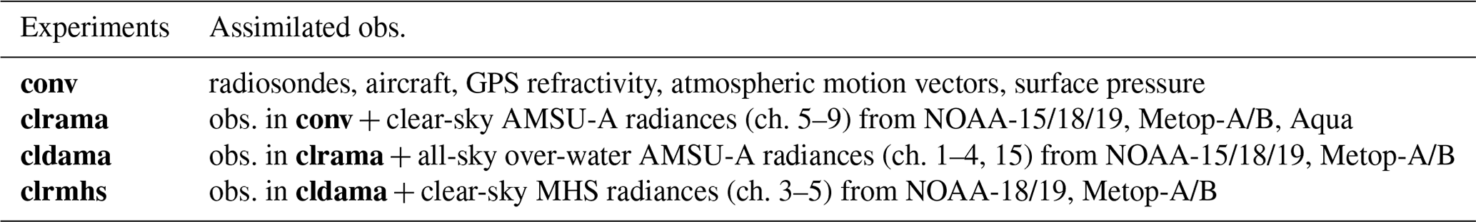
The four experiments differ from each other by assimilating different sets of observations, as listed in Table 1. The conv experiment assimilates temperature, specific humidity, and zonal and meridional wind components from radiosondes and aircraft; GPS refractivity; atmospheric motion vectors (AMVs) retrieved from geostationary and polar-orbiting satellite sensors; and surface pressure (p_s). In addition to the observations used in conv, the clrama experiment assimilates clear-sky AMSU-A radiances (channels 5–9) from six satellites (NOAA-15/18/19, Metop-A/B, Aqua; omitting platforms and channels that had failed before the experimental period). The cldama experiment further adds over-water AMSU-A window channels (channels 1–4 and 15) all-sky radiances from five satellites. Note that Aqua AMSU-A channels 1 and 2, which are needed for the all-sky observation error model (see Sect. 3.4), are not available, and thus Aqua AMSU-A window channels are excluded in cldama. We use the fourth experiment, clrmhs, to evaluate the additional benefit of assimilating three water vapor channels from the Microwave Humidity Sounder (MHS) on board four satellites (NOAA-18/19, Metop-A/B) under clear-sky conditions. Data thinning is applied to AMSU-A and MHS radiance data with a 145 km thinning mesh. All four experiments use a ±3 h time window.

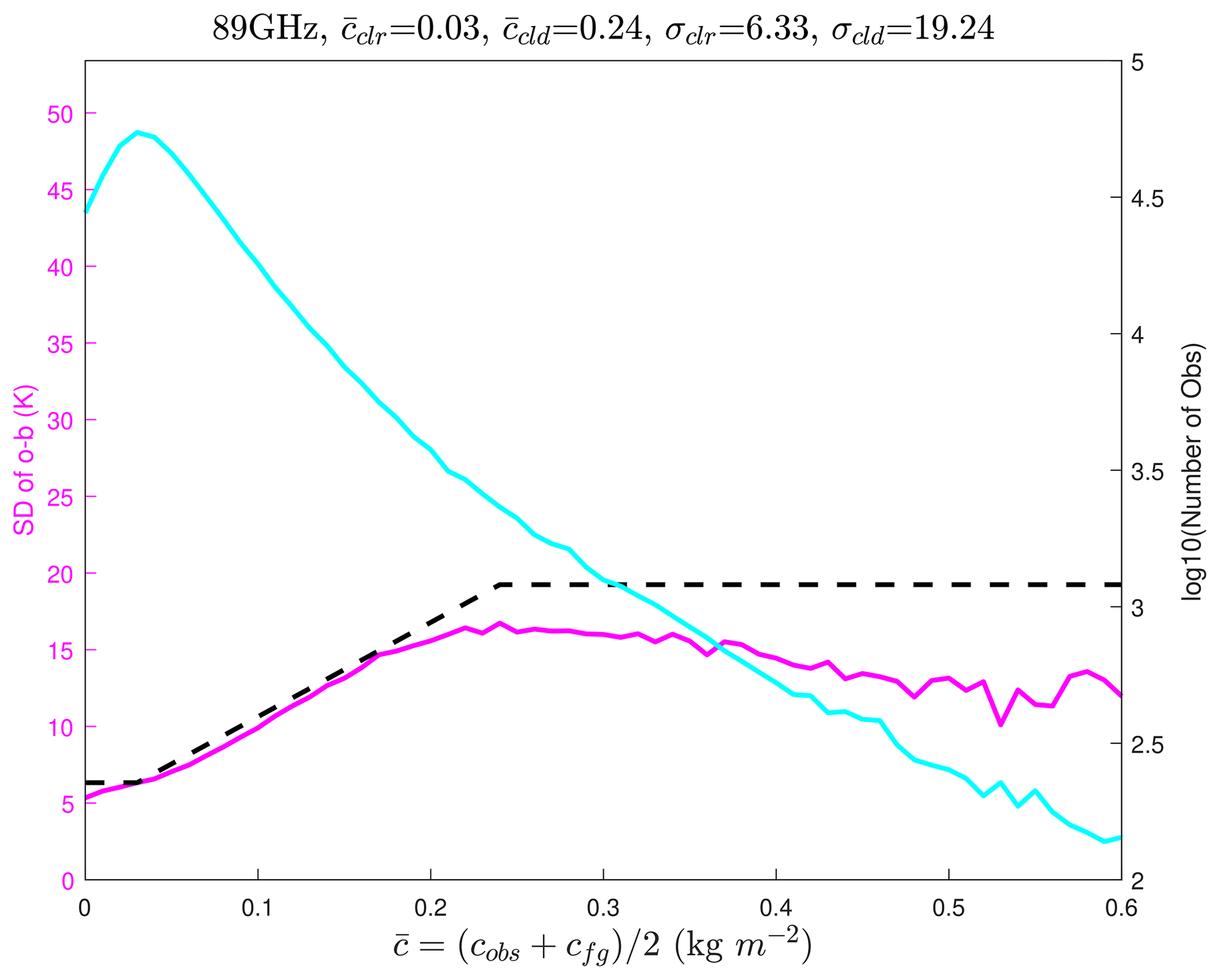
Figure 1 All-sky observation error model for NOAA-19 AMSU-A channel 15. The magenta curve is the statistics of the standard deviation of O minus B (left y axis) as a function of the model–observation-averaged cloud liquid water path (x axis). The cyan curve gives the number of observations (right y axis) used in each bin's statistics (0.01 kg m⁻² bin interval). The dashed black curve is the fitted piecewise-linear ramp function of the magenta curve, serving as the all-sky observation error model. Variables in the title are those of Eq. (11) in Sect. 4.

All-sky observation error statistics were computed separately for five AMSU-A sensors using the observations minus the CRTM-simulated brightness temperatures from the 6 h forecast background fields (i.e., O minus B) of the clrama experiment over the month-long period. Figure 1 gives an example of the all-sky observation error model for NOAA-19 AMSU-A channel 15 at 89 GHz. The blue curve is the statistics of the standard deviation of O minus B as a function of the model–observation-averaged cloud liquid water path $\stackrel{\mathrm{‾}}{c}=(c_{\mathrm{obs}}+c_{\mathrm{fg}})/\mathrm{2}$. The red curve gives the number of observations (the right y axis) used in each bin's statistics (0.01 kg m⁻² bin interval). The dashed black curve is the fitted piecewise-linear ramp function of the blue curve in the form (Geer and Bauer, 2011)

$$\begin{array}{}\text{(11)}& {\mathit{\sigma }}_{\mathrm{o}}=\left\{\begin{array}{lr}{\mathit{\sigma }}_{\mathrm{clr}},& \text{if }\stackrel{\mathrm{‾}}{c}\le {\stackrel{\mathrm{‾}}{c}}_{\mathrm{clr}}\\ {\mathit{\sigma }}_{\mathrm{clr}}+({\mathit{\sigma }}_{\mathrm{cld}}-{\mathit{\sigma }}_{\mathrm{clr}})\frac{\stackrel{\mathrm{‾}}{c}-{\stackrel{\mathrm{‾}}{c}}_{\mathrm{clr}}}{{\stackrel{\mathrm{‾}}{c}}_{\mathrm{cld}}-{\stackrel{\mathrm{‾}}{c}}_{\mathrm{clr}}},& \text{if }{\stackrel{\mathrm{‾}}{c}}_{\mathrm{clr}}<\stackrel{\mathrm{‾}}{c}\le {\stackrel{\mathrm{‾}}{c}}_{\mathrm{cld}}\\ {\mathit{\sigma }}_{\mathrm{cld}},& \text{if }\stackrel{\mathrm{‾}}{c}>{\stackrel{\mathrm{‾}}{c}}_{\mathrm{cld}}\end{array}\right.,\end{array}$$

which serves as the observation error model for this particular channel with ${\stackrel{\mathrm{‾}}{c}}_{\mathrm{clr}}=\mathrm{0.03}$, ${\stackrel{\mathrm{‾}}{c}}_{\mathrm{cld}}=\mathrm{0.24}$, σ_clr=6.33, and σ_cld=19.24. The four numbers for each of channels 1–4 and 15 of five AMSU-A sensors are provided in the supplemental configuration file of JEDI-MPAS (jedi_mpas.yaml in the Supplement), which specifically describes the configuration for the clrmhs experiment.

BUMP has the ability to diagnose horizontal and vertical localization length scales with geographical variation. For a relatively small ensemble size, however, BUMP-diagnosed localization length scales may not be optimal. Therefore, we used the fixed localization scale values in this study, which is not uncommon for ensemble DA. After some sensitivity testing, we use 1200 and 6 km for the horizontal and vertical full widths of Gaspari and Cohn (1999) localization function (Eq. 4.10), respectively. That function reduces the spatial correlation to zero when the distance between two locations is greater than the full width.

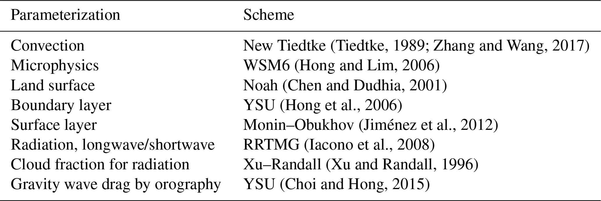
The MPAS-A model is configured with a 30 km quasi-uniform mesh and 55 vertical levels with a 30 km model top. The “mesoscale reference” physics suite is used with the parameterization schemes listed in Table 2. A time step of 180 s is applied for the model time integration. We used the same “mesoscale reference” physics suite to generate the 6 h MPAS ensemble forecasts on the 60 km mesh that comprise the sample ensemble covariances.

(Tiedtke, 1989; Zhang and Wang, 2017)(Hong and Lim, 2006)(Chen and Dudhia, 2001)(Hong et al., 2006)(Jiménez et al., 2012)(Iacono et al., 2008)(Xu and Randall, 1996)(Choi and Hong, 2015)

Table 2 Parameterization schemes in the “mesoscale reference” physics suite.

5 Evaluation results

5.1 Short-term forecasts

Here we assess the DA cycling performance of the four experiments by examining the first-guess departure (i.e., observation minus background or OMB) statistics, similar to the diagnostic commonly monitored at operational NWP centers (e.g., https://www.ecmwf.int/en/forecasts/charts/obstat/, last access: 21 October 2022). Additionally, we present error statistics of 6 h forecast backgrounds with respect to the NCEP's GFS analysis to more clearly assess the geographic and vertical variations of the cycling performance.

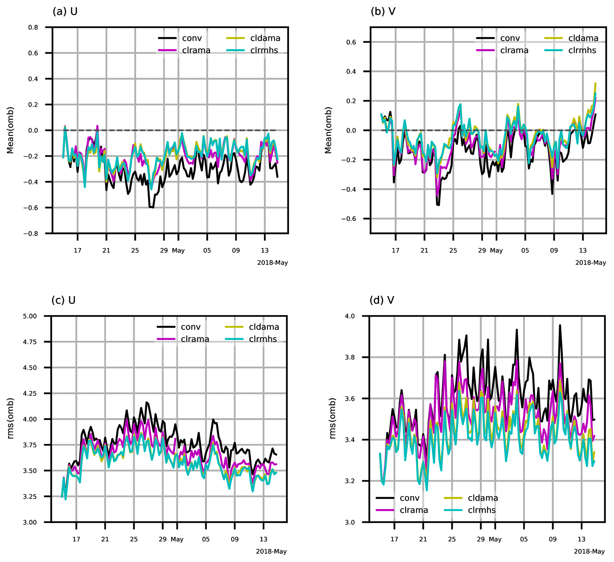
Figure 2 Time series (00:00 UTC, 15 April–18:00 UTC, 14 May 2018) of (a, b) mean and (c, d) rms of OMB for AMV (a, c) zonal and (b, d) meridional wind components (units: m s⁻¹) from the four experiments. The background is a 6 h forecast. Statistics are computed over the globe and averaged for all vertical levels.

5.1.1 Observation space verification

Figure 2 displays time series of mean and root mean square (rms) values of OMB for AMV zonal and meridional wind components from the four experiments. Overall the mean and rms give the consistent performance indication for the four experiments. For zonal wind, the conv experiment has the largest bias and root mean square error (RMSE); adding clear-sky AMSU-A radiances leads to substantial error reduction in terms of both bias and RMSE; further adding all-sky AMSU-A window-channels' radiances additionally reduces the RMSE. The red curves (clrmhs) are basically overlaid with the green curves (cldama), indicating a neutral impact on 6 h wind forecasts by adding clear-sky MHS water vapor radiances to all-sky AMSU-A radiances. The statistics of OMB for AMV meridional wind component indicate similar relative experiment performances overall, except for a slightly positive impact for clrmhs versus cldama.

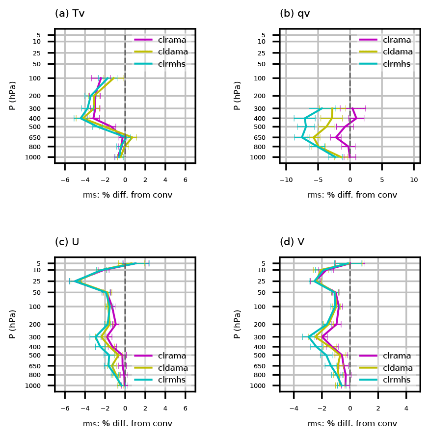
Figure 3 Vertical distributions of relative rms reduction of OMB for radiosondes' (a) virtual temperature, (b) specific humidity, (c) zonal wind, and (d) meridional wind. Statistics are computed over the period from 00:00 UTC, 18 April, to 18:00 UTC, 14 May 2018, for the three radiance DA experiments against the conv experiment. A negative percentage indicates the positive impact from radiance DA experiments relative to the non-radiance DA experiment.

Figure 3 compares the 6 h forecast fits to radiosonde observations from the three radiance DA experiments with those of the conv experiment. Shown in Fig. 3 are relative differences between rms of OMB from the three radiance DA experiments and that from the conv experiment, given by

$$\begin{array}{}\text{(12)}& \text{ratio}=\mathrm{100}\times ({\mathrm{rms}}_{\mathrm{EXP}}-{\mathrm{rms}}_{\mathrm{conv}})/{\mathrm{rms}}_{\mathrm{conv}},\end{array}$$

where “EXP” can be clrama, cldama, or clrmhs. Negative ratios indicate positive impacts from EXP relative to conv, and vice versa. Different magnitudes of ratio among the three radiance experiments give their relative performance. A 95 % confidence interval is shown at each pressure level as an error bar, which is computed using bootstrap resampling (Hamill, 1999), with a resample size of 10 000. The rms difference between EXP and conv at each cycle is treated as an independent sample in the bootstrap. Assimilating clear-sky temperature sounding channels from clrama has small impacts on humidity (blue curve in Fig. 3b), whereas large positive impacts on moisture are obtained by adding all-sky AMSU-A and clear-sky MHS radiances. The impact on virtual temperature (T_v) is mostly from AMSU-A clear-sky temperature sounding channels, and the additional benefit on T_v from all-sky AMSU-A and clear-sky MHS radiances is relatively small (Fig. 3a). The reason we show T_v here instead of T is that the majority of radiosonde temperature observations in GSI's ncdiag files are expressed in terms of T_v. The rms decreases up to 5 % for zonal wind (Fig. 3c) and 2 % for meridional wind (Fig. 3d) from clrama, likely caused by the mass–wind balance implied in the ensemble background error covariance. The extra benefit on wind fields from AMSU-A all-sky window channel radiances is confined to 200–800 hPa. Additional positive impact on winds between 300 and 650 hPa is achieved by adding MHS clear-sky water vapor channels' radiances. Each of the three radiance DA experiments exhibit, to a different extent, improvement with respect to the conv experiment for all four observed radiosonde variables at almost all pressure levels.

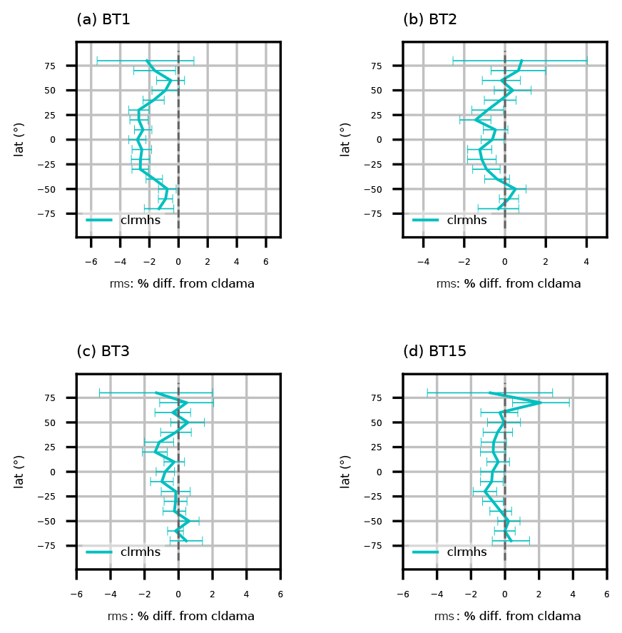
Figure 4 Similar to Fig. 3 but for latitudinal variation of relative rms reduction of OMB for NOAA-19 AMSU-A ch. 1–3 and 15 for clrmhs versus cldama.

Among the four experiments, both cldama and clrmhs assimilate AMSU-A all-sky radiances from the window channels (ch. 1–4 and 15). It is expected a priori that assimilating MHS water vapor channels' radiances in clrmhs will improve background fitting to those AMSU-A all-sky radiances. That is indeed the case in Fig. 4; clrmhs achieves statistically significant improvement up to 2.5 % at tropical latitudes for AMSU-A channel 1 (Fig. 4a), while positive impacts from MHS radiances are smaller and less significant for other AMSU-A window channels (Fig. 4b–d). This is because AMSU-A channel 1 (23.8 GHz) is more sensitive to water vapor and clouds than other AMSU-A window channels.

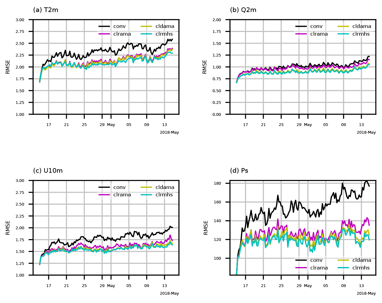
Figure 5 Time series (00:00 UTC, 15 April–18:00 UTC, 14 May 2018) of RMSE of cycling background with respect to GFS analyses for global (a) temperature (units: kelvin) and (b) specific humidity (units: g kg⁻¹) at 2 m, (c) zonal wind component (units: m s⁻¹) at 10 m, and (d) surface pressure (units: Pa) from the four experiments.

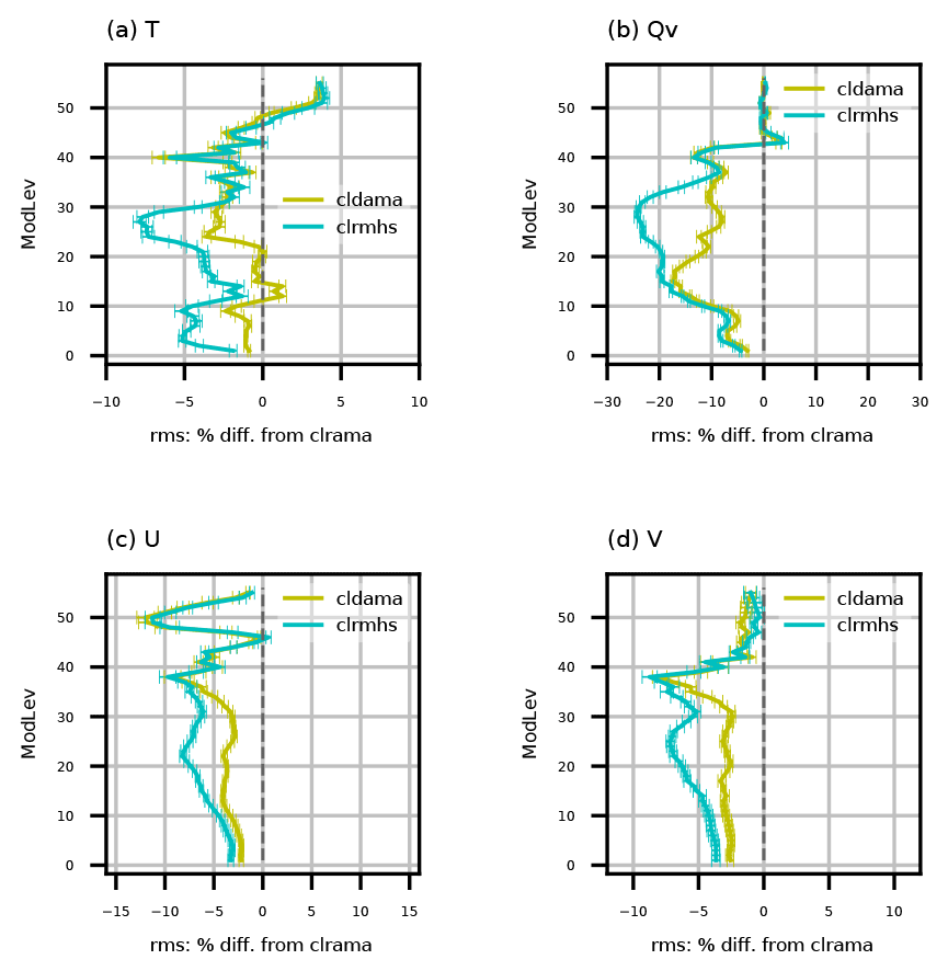
Figure 6 Vertical distributions of relative RMSE reduction (with respect to GFS analyses) of cycling background for global (a) temperature, (b) water vapor mixing ratio, (c) zonal wind, and (d) meridional wind (cldama and clrmhs versus clrama). Statistics are for the period from 00:00 UTC, 18 April, to 18:00 UTC, 14 May 2018.

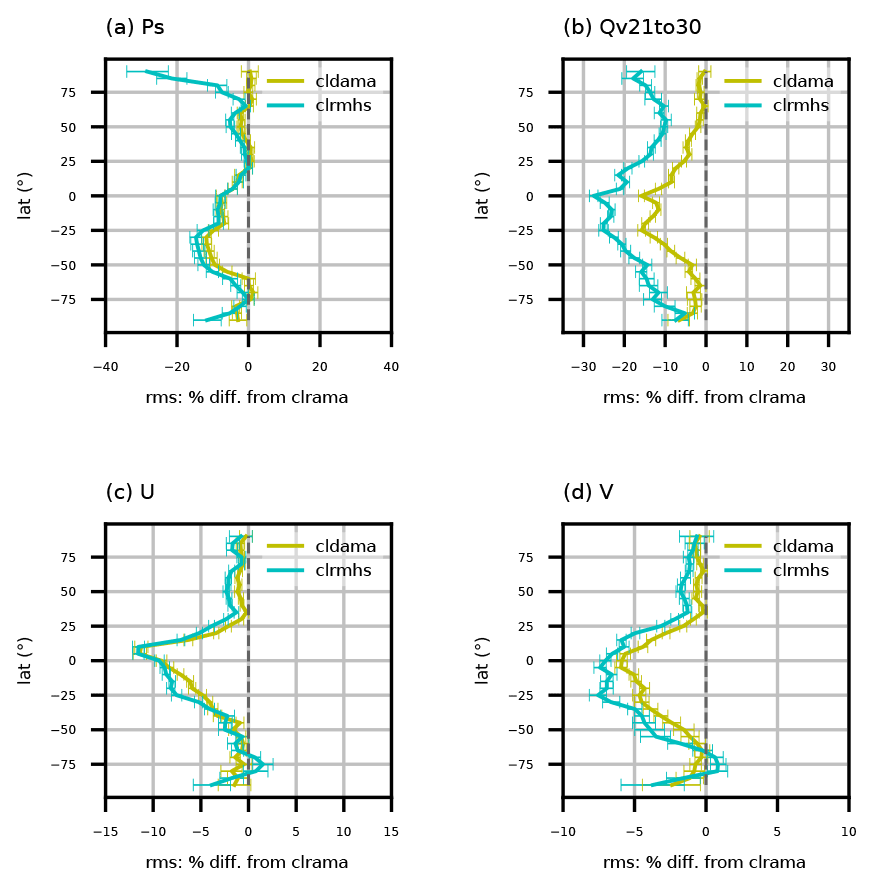
Figure 7 Similar to Fig. 6 but for latitudinal variations of RMSE reduction for (a) surface pressure, (b) water vapor mixing ratio of model level 21 to 30, and the whole-column (c) zonal wind and (d) meridional wind.

5.1.2 Model space verification

Similar to Figs. 2–4, Figs. 5–7 evaluate the 6 h forecast backgrounds in model space relative to GFS analyses. Figure 5 shows the time series of global RMSE of the four experiments for four surface variables. Note that the background for the first analysis at 00:00 UTC, 15 April 2018, is a 6 h forecast initialized from the GFS analysis. GFS utilizes a hybrid-4DEnVar DA technique via the GSI system (Kleist and Ide, 2015) and includes assimilation of many more satellite observations than those used in our own cycling experiments. Smaller RMSEs for the first 2–3 d come from the memory of the superior performance of the operational analysis. Cycling performance quickly converges to a stable level for the three radiance DA experiments due to the good global coverage of observations. Gradually increasing errors are clearly seen in the conv experiment for 2 m temperature (T₂), 10 m zonal wind (u₁₀), and p_s, which is caused by sparse coverage of non-radiance data over the Southern Hemisphere. The impacts of AMSU-A clear-sky and all-sky radiances and MHS clear-sky radiances are consistent with those shown in upper-air observation space of Fig. 3.

Similar to Fig. 3, Fig. 6 presents the vertical distribution of the global percentage RMSE difference of cldama and clrmhs relative to clrama. Figure 6 yields similar conclusions as Fig. 3, but the magnitudes of improvement in model space (Fig. 6) are larger than those in observation space (Fig. 3) because the model space verification covers the entire globe. The most drastic improvement is for water vapor mixing ratio, with nearly 20 % RMSE decrease at model level 15 (∼2.2 km or ∼700 hPa) by assimilating AMSU-A all-sky radiances and >20 % improvement at model level 30 (∼8.8 km or ∼330 hPa) when adding both AMSU-A all-sky radiances and MHS clear-sky radiances (Fig. 6b). One noticeable issue is the negative impact for temperature near the model top (Fig. 6a), which is believed to be related to an increasing cold bias during the cycling (not shown). A biased model top makes radiance DA less effective. Note that the MPAS-A model currently lacks processes for representing O₃ chemistry and that a climatological O₃ field is used, leading to inaccurate radiation calculations attributed to O₃. Work is underway to add a parameterized O₃ chemistry scheme (McCormack et al., 2006) and include O₃ as a prognostic variable in MPAS-A.

Figure 7 is similar to Fig. 6 but depicts the latitudinal variation of relative RMSE reduction for several variables. For p_s, the greatest impact is between 25–50^∘ S (Fig. 7a), and large RMSE reductions are also seen in North and South Pole regions for the clrmhs experiment (Fig. 7a). The large RMSE reduction from clrmhs in the Arctic is apparently associated with a reduction of a ∼1 hPa low pressure bias in the conv, clrama, and cldama experiments (not shown). For the other three variables, the greatest impact is within tropical regions (Fig. 7b–d). In addition to the large benefit on moisture from the addition of MHS water vapor channels' radiances (Fig. 7b), the impact of MHS radiances on the meridional wind component (Fig. 7d) is also substantial and significant, possibly indicating an improved representation of equatorial convergence–divergence patterns associated with convective activity.

These observation-space and model-space evaluations of short-term forecasts demonstrate that the JEDI-MPAS 3DEnVar scheme behaves well for the assimilation of clear-sky and all-sky microwave radiance data. More accurate background fields are obtained by adding more and more radiance data.

5.2 The 1–10 d forecasts

This subsection examines the 1–10 d forecast performance relative to GFS analyses, independent radiance data from the Advanced Himawari Imager (AHI), and a global precipitation product. A total of 27 10 d forecasts initialized each day at 00:00 UTC from 18 April to 14 May 2018 are used to produce the error statistics. The first 3 d (15–17 April) is considered the spin-up period for each experiment to converge from the GFS climatology to JEDI-MPAS's own cycling climatology and thus are not included in the forecast evaluation. The three radiance DA experiments significantly outperform the conv experiment. Therefore, we only evaluate the cldama and clrmhs experiments, from here considering the clrama experiment as the benchmark.

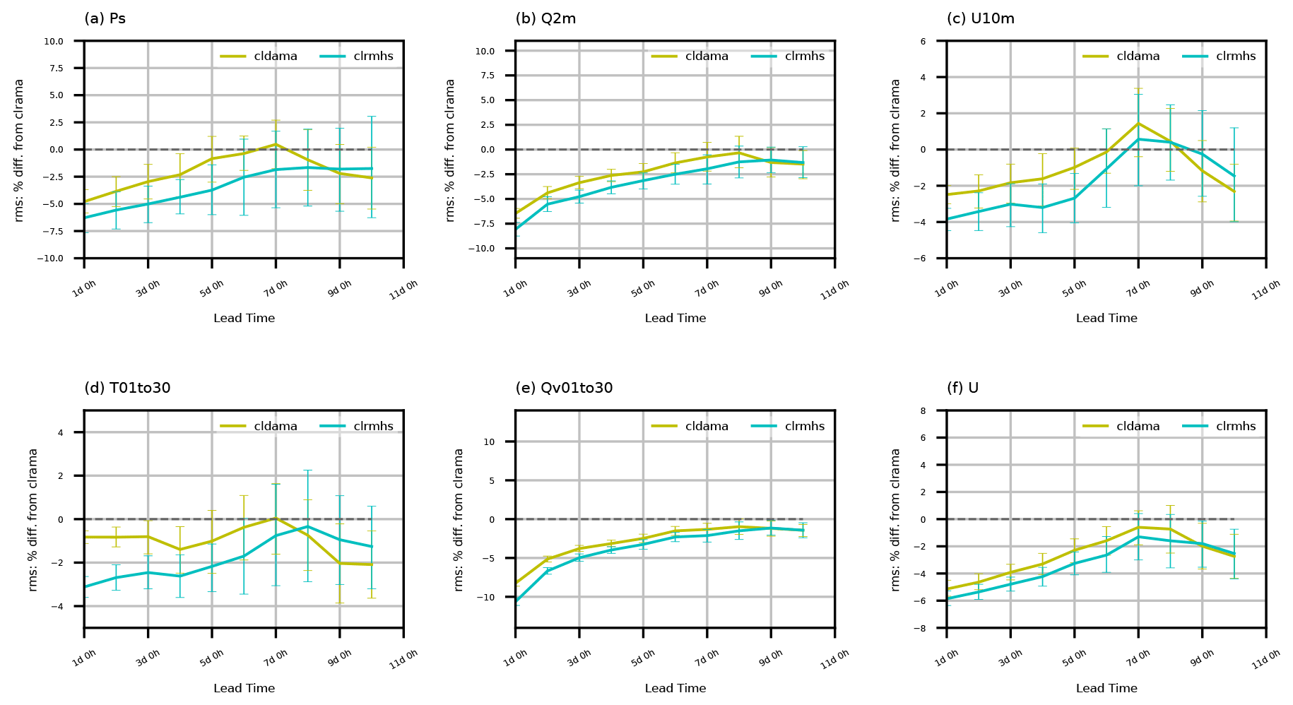
Figure 8 Relative RMSE reductions (with respect to GFS analyses) as a function of forecast lead time for global (a) surface pressure, (b) specific humidity at 2 m, (c) zonal wind at 10 m, (d) temperature and (e) water vapor mixing ratio below model level 30, and (f) the whole-column zonal wind (cldama and clrmhs versus clrama). Statistics are aggregated over all 27 forecasts.

5.2.1 Model space verification

Figure 8 displays relative RMSE reductions (with respect to GFS analyses) as a function of forecast lead time for three surface and three upper-air variables. Due to a temperature bias at the model top, as described in Sect. 5.1 in relation to Fig. 6a, the evaluation on temperature is limited to below model level 30. We also exclude the moisture assessment above model level 30, where the air is very dry. In general, adding AMSU-A all-sky radiances produces more accurate forecasts for all variables compared to the AMSU-A clear-sky radiance experiment, and extra MHS clear-sky radiances further reduce forecast errors. Percentage improvements and associated statistical significance decrease with forecast range but can last up to 10 d, especially for the clrmhs experiment. Note that forecast errors increase with forecast lead time, and thus absolute error reduction could be increased or flat at certain forecast lead times, even with decreasing percentage improvement. The greatest improvement from clrmhs is for upper-air moisture with up to 10 % and >1 % RMSE reduction for day 1 and day 10, respectively (Fig. 8e). The improvement for moisture remains statistically significant for the whole 10 d forecast range, while that is not the case for other variables. This result is consistent with AMSU-A window channels' and the three MHS channels' large sensitivity to water vapor (and clouds for AMSU-A all-sky radiances). Large impacts are also seen on Q2m (Fig. 8b), though to a lesser extent than is seen for upper-air moisture. Conversely, the impact is the smallest on temperature (Fig. 8d), with only ∼1 % and 3 % improvement for the day 1 forecast from cldama and clrmhs, respectively. The magnitudes of improvement on p_s and the zonal wind are comparable to each other, gradually decreasing from an initial ∼5 % rms reduction for the day 1 forecast.

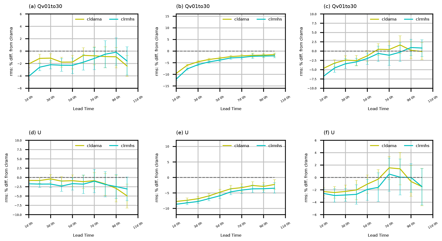
Figure 9 Similar to Fig. 8 but for water vapor mixing ratio below model level 30 and zonal wind over the three regions (30–90^∘ N, 30^∘ S–30^∘ N, and 30–90^∘ S).

Figure 9 shows the impact on moisture and zonal wind over three different regions. The largest impact is over the tropical region for both variables, which is consistent with the short-term forecast impact as shown in Fig. 7b and c. The smallest impact is between 30 and 90^∘ N, where conventional observations have good coverage. One interesting thing is that the impact over the tropics exhibits a clear decreasing trend with forecast range, but this decreasing trend is not always present poleward of 30^∘. This might be related to the different levels of convective weather activity between low and middle/high latitudes.

Figure 10 Similar to Fig. 8 but for clrmhs versus clrdma of four upper-air variables.

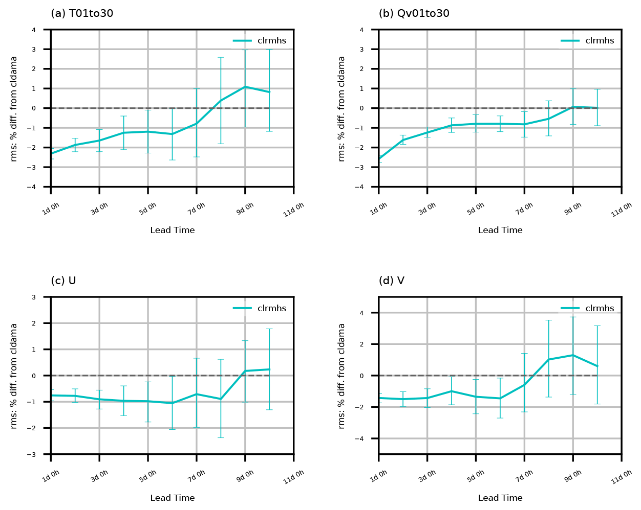
Figure 10 more clearly depicts the relative impact of clrmhs with respect to cldama for four upper-air variables. Again, the greatest and most significant improvement (up to 7 d) achieved by adding MHS water vapor channels' radiances is on moisture with 2.5 % RMSE reduction for day 1 and still retaining ∼1 % for day 7 (Fig. 10b). The magnitude of MHS radiance impact on temperature (Fig. 10a) is comparable with that of moisture but less statistically significant. The MHS impact on the wind field is smaller, but the percentage of improvement remains nearly unchanged, with the forecast lead time for up to day 8 for zonal wind (Fig. 10c) and day 6 for meridional wind (Fig. 10d). Similar to the impact on short-term forecasts shown in Fig. 7, the MHS radiance impact on meridional wind (∼1.5 %) is 50 % greater than that for the zonal wind (∼1 %) up to day 6.

5.2.2 Verification against AHI radiances

JEDI-MPAS also has the capability of simulating and assimilating clear-sky and cloudy infrared (IR) radiances such as those from the geostationary satellite sensor Advanced Himawari Imager (AHI). CRTM's cloudy IR radiance simulation capability with JEDI-MPAS is used to evaluate 1–10 d forecasts using independent (i.e., not assimilated) AHI full-disk radiance data centered at 140.7^∘ E. Using the JEDI-MPAS HofX3D application, and in conjunction with UFO, CRTM takes the forecast temperature, moisture, and hydrometeor profiles at AHI locations to compute modeled AHI radiances. Then we compare the simulated and observed AHI brightness temperatures offline. Before being ingested into JEDI-MPAS, the raw AHI IR channels' data at 2 km resolution undergo cloud detection at each pixel following Wu et al. (2020) and are preprocessed into super-observations averaged over 15×15 pixels. The cloud detection and superobbing are carried out offline using WRFDA. These super-observations better match the model's 30 km mesh, reducing representativeness errors. A by-product of cloud detection on the raw AHI pixels and superobbing is the cloud fraction for each super-observation, which allows for statistical evaluation separately over clear, partly cloudy, and overcast observations.

Figure 11 Similar to Fig. 8 but for RMSE in AHI's six channels' brightness temperature space.

Figure 11 shows the relative RMSE reduction as a function of forecast range in AHI radiance space for all superobbed pixels of six channels. Among them, channels 8–10 are water vapor (WV) channels sensing the middle-to-upper tropospheric moisture, and bands 13–15 are window channels sensitive to surface properties and clouds. The patterns of the RMSE reduction across different channels are very similar and overall consistent with those in the model space variables shown in Figs. 8 and 9. The impact of cldama and clrmhs for the higher peaking channel 8 (350–400 hPa) is larger than that for the lower peaking channel 10 (600–700 hPa), which is consistent with the vertical distribution of humidity RMSE reduction shown in Fig. 6b. Improved fitting to the three window channels (relative to clrama) is most likely evidence of improved cloud forecasts, with significance at least up to day 4. Figure 12 further splits error statistics into clear, partly cloudy, and fully cloudy pixels for the lower peaking WV channel 10. Over the verification period, clear, partly cloudy, and fully cloudy pixels account for 28 %, 33 %, and 39 % of observations, respectively. The relative impact from cldama and clrmhs decreases with more cloudiness. The absolute RMSE reduction, however, is comparable for the three categories due to increased RMSE with more cloudiness.

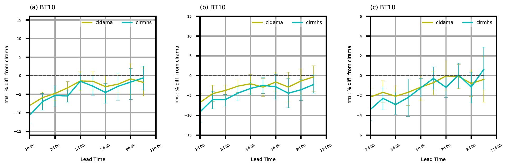
Figure 12 Similar to Fig. 11 but for AHI channel 10's error statistics over (a) clear, (b) partly cloudy, and (c) fully cloudy pixels, respectively.

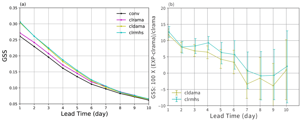
Figure 13 (a) Gilbert skill scores (GSSs) of 24 h accumulated precipitation forecast verified against CMORPH observations for a threshold of 10 mm. (b) Relative difference of GSSs between $\mathbf{cldama}/\mathbf{clrmhs}$ and clrama, also for a threshold of 10 mm.

5.2.3 Precipitation forecast verification

The 24 h accumulated precipitation forecasts from the four experiments are verified against the Climate Prediction Center's morphing technique (CMORPH) 0.25^∘ precipitation product (Xie et al., 2017). Figure 13a gives the Gilbert skill scores (GSSs) (also known as equitable threat scores, ETSs) (Hogan et al., 2010) computed for the observed and predicted 24 h accumulated rainfall ≥10 mm using the Model Evaluation Tool (MET) (Brown et al., 2021). The GSS ranges from $-\mathrm{1}/\mathrm{3}$ to 1, with ≤0 corresponding to no skill and 1 to perfect skill. An improvement of 5 %–8 % is gained up to day 7 precipitation forecast from AMSU-A temperature-sounding radiance DA when compared to the non-radiance DA experiment. A further 5 %–12 % improvement is achieved by adding AMSU-A all-sky radiances and MHS radiances for up to day 6 (Fig. 13b). From precipitation forecast verification here and other aspects of forecast verification shown earlier, JEDI-MPAS's AMSU-A all-sky DA exhibits a larger positive impact than that at operational centers (e.g., Zhu et al., 2016; Migliorini and Candy, 2019). This might be partly related to the use of the full all-sky approach in JEDI-MPAS, whereas Zhu et al. (2016) and Migliorini and Candy (2019) assimilated AMSU-A all-sky radiances only under non-precipitating conditions. Also, obtaining additional benefit above a well-tuned operational system with abundant satellite observations, as in Zhu et al. (2016) and Migliorini and Candy (2019), is much harder than for the benchmark experimental settings used in this study.

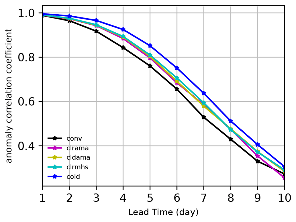
Figure 14 Global anomaly correlation coefficients of 500 hPa geopotential height as a function of forecast lead time for the four cycling experiments together with the cold-start forecasts initialized from GFS analyses (blue).

5.2.4 Anomaly correlation coefficient for 500 hPa geopotential height

Figure 14 provides global anomaly correlation coefficients (ACCs) of 500 hPa geopotential height as a function of forecast range for the four JEDI-MPAS experiments together with the cold-start forecast experiment using GFS analyses as initial conditions (light blue, marked as cold). The climatology derived from the 1980–2010 NCEP/NCAR reanalysis products (Kalnay et al., 1996) is used in the ACC calculation. The largest improvement on ACC is from AMSU-A temperature sounding channels, gaining a half day of skill (from 4.5 to 5 d) with respect to the non-radiance experiment for 0.8 ACC level. Further ACC improvement by adding AMSU-A all-sky window channels and MHS clear-sky WV channels is visible but much smaller than that gained by AMSU-A clear-sky temperature-sensitive channels. This could be understandable with the tight link between temperature and geopotential height. The cold-start forecasts from GFS analyses reach 5.5 d for 0.8 ACC level and outperforms JEDI-MPAS's three radiance DA experiments by half a day. Given that the operational GFS analysis is produced with a more advanced hybrid-4DEnVar algorithm (Kleist and Ide, 2015) at a higher resolution and with ensemble covariances formed by 80-member ensemble input, plus the assimilation of many more satellite observations, this half-day gap on ACC is not surprising with a less advanced pure 3DEnVar algorithm, a smaller ensemble size, and fewer observations assimilated in JEDI-MPAS experiments.

6 Conclusions and future perspectives

A new DA system for the MPAS-A model has been developed based upon the JEDI software framework and was publicly released as JEDI-MPAS 1.0.0 for community use. This article describes the EnVar's formulation and technical implementation of JEDI-MPAS and evaluates its robustness and performance through four global cycling 3DEnVar experiments. JEDI-MPAS is robust, with stable cycling over a month-long period, and behaves well, with positive impacts obtained when adding more and more microwave radiance data for most aspects of assessment in both observation and model space. One advanced feature developed with JEDI-MPAS is all-sky radiance DA capability along with the introduction of hydrometeor analysis variables, which is first applied to the assimilation of all-sky radiances from AMSU-A's five window channels. Large impacts are achieved from AMSU-A all-sky DA, especially for moisture, clouds, and precipitation forecasts. Credible forecast skill is seen from the assimilation of a subset of conventional and satellite observations used in operational NWP centers, with a half-day skill gap relative to forecasts initialized from GFS analyses for the 0.8 ACC level of 500 hPa geopotential height. It is expected that the forecast performance can be further improved to be closer to operational skill using a more advanced DA algorithm such as 4DEnVar, a larger ensemble size, more satellite data, a higher model resolution, and fine tuning of DA settings, as well as by improving the MPAS model. JEDI-MPAS can also perform deterministic analyses using 3DVar and ensemble analyses using the EDA technique. The implementation and evaluation of 3DVar and EDA will be described in separate articles. JEDI-MPAS in regional mode and with a variable resolution will also be evaluated with higher resolutions.

The general JEDI software framework and more specific JEDI-MPAS DA system are still undergoing active development since the JEDI-MPAS 1.0.0 release. One new development specific to JEDI-MPAS is to change the hydrostatic balance constraint in the full fields to the increment fields, which can still allow surface pressure observations to constrain the upper-air variables but is better suited for the non-hydrostatic MPAS-A model. Initial tests of this new linear hydrostatic balance constraint show improvement, especially near the model top. Other ongoing work on the model side is to introduce a parameterized O₃ chemistry scheme (McCormack et al., 2006) and include O₃ as a prognostic variable in MPAS-A, which should reduce temperature bias in the stratosphere and also allow for the assimilation of satellite-based O₃ observations. Improving stratosphere processes will allow the use of a high model top, which will enable the assimilation of higher-peaking radiance data. All-sky radiance DA for both microwave and infrared sensors continues to be refined with JEDI-MPAS. One important feature missing in the released JEDI/UFO but available in the “develop” branch of the UFO is the variational bias correction (VarBC) for satellite radiance data (Auligné et al., 2007; Dee and Uppala, 2009; Zhu et al., 2013), which is undergoing active testing and evaluation with JEDI-MPAS at the time of writing. The quality control procedures of several types of observations implemented in the UFO are also being tested with assimilation of raw NCEP-bufr converted observation input files, with the goal of eliminating reliance on GSI for quality control. Moreover, the computational efficiency of JEDI is being improved. We intend to periodically release new and improved versions of JEDI-MPAS in upcoming years.