the Creative Commons Attribution 4.0 License.
the Creative Commons Attribution 4.0 License.
 | 17 Oct 2022
Recovery of sparse urban greenhouse gas emissions
Man Sun
Florian Dietrich
To localize and quantify greenhouse gas emissions from cities, gas concentrations are typically measured at a small number of sites and then linked to emission fluxes using atmospheric transport models. Solving this inverse problem is challenging because the system of equations often has no unique solution and the solution can be sensitive to noise. A common top–down approach for solving this problem is Bayesian inversion with the assumption of a multivariate Gaussian distribution as the prior emission field. However, such an assumption has drawbacks when the assumed spatial emissions are incorrect or not Gaussian distributed. In our work, we investigate sparse reconstruction (SR), an alternative reconstruction method that can achieve reasonable estimations without using a prior emission field by making the assumption that the emission field is sparse. We show that this assumption is generally true for the cities we investigated and that the use of the discrete wavelet transform helps to make the urban emission field even more sparse. To evaluate the performance of SR, we created concentration data by applying an atmospheric forward transport model to CO2 emission inventories of several major European cities. We used SR to locate and quantify the emission sources by applying compressed sensing theory and compared the results to regularized least squares (LSs) methods. Our results show that SR requires fewer measurements than LS methods and that SR is better at localizing and quantifying unknown emitters.
- Article
(8700 KB) - Full-text XML
-
Supplement
(374 KB) - BibTeX
- EndNote


Understanding anthropogenic greenhouse gas (GHG) emissions is important for scientists and decision makers fighting climate change. Based on a growing amount of atmospheric observations, studies estimating emission fields of GHG sources and sinks from these observations have been performed on local (Chen et al., 2016; Viatte et al., 2017; Toja-Silva et al., 2017), metropolitan (Jones et al., 2021; Turner et al., 2020; Hase et al., 2015), country (Miller et al., 2013; Shekhar et al., 2020), and global (Hirsch et al., 2006; Mueller et al., 2008; Turner et al., 2015; Jacob et al., 2016) scales. One of the main reasons for such studies is to verify and improve GHG emission inventories created by bottom–up methods. Verification and improvements include but are not limited to
-
determining the difference between the real emissions and the emissions captured by inventories
-
determining differences between the real and bottom–up estimated emissions for individual emitters
-
finding emitters which are not captured by inventories (unknown emitters).
Atmospheric inverse modeling methods use column or in situ GHG concentration measurements to estimate emission fields. Due to a lack of measurements and high modeling and measurement uncertainties, estimating each grid cell of an emission field independently is not possible. Instead, sectors (Jones et al., 2021), spatial correlations (Wesloh et al., 2020), and/or temporal correlations (Jones et al., 2021; Wesloh et al., 2020) are used to construct alternative parameterizations of emission fields to prevent overfitting.
An alternative to overcoming these issues are sparse reconstruction (SR) methods (Ray et al., 2015). SR methods can use concentration measurements to estimate sparse emission fields, meaning that only a small number of large emitters contribute significantly to the total emissions. These methods determine the critical emission grid cells and adjust the emissions of only those cells until the model best matches the observations. All other grid cells are set to zero. Once conditions of compressed sensing (CS) are fulfilled, SR methods are guaranteed to determine the best possible emission fields and provide a good estimation of their emissions.
SR for the recovery of GHGs has been proposed by several recent studies. Ray et al. (2014, 2015) used stagewise orthogonal matching pursuit (StOMP), a reconstruction method known from compressed sensing, and modified it to enforce positive emission estimates. To overcome the restriction of sparse reconstruction of only being able to reconstruct sparse fields, they used a multi-scale resolution field based on wavelets. In Ray et al. (2015), StOMP has been modified so that prior information can be included. Both studies reconstructed fossil fuel CO2 emissions in an idealized scenario with synthetic measurements and very low measurement noise (SNR >40 dB). Hase et al. (2017) demonstrated sparse reconstruction with enforced positive emission estimates of anthropogenic CH4 emissions from synthetic observations in the US. To increase the sparsity of the emission field, Hase et al. (2017) used a redundant dictionary representation, where the representation of the emission field is not unique. Yan et al. (2012) proposed compressed sensing, i.e., sparse reconstruction with guaranteed best feature selection, for environmental monitoring with the focus on undersampling.
In this paper, we apply SR to assessing urban GHG emissions. Current GHG emission monitoring systems in cities, such as Dietrich et al. (2021), Shusterman et al. (2016) and Sargent et al. (2018), acquire GHG concentration in the atmosphere as column or in situ concentration measurements. These measurements are then related to city emissions and background concentrations, where the city emissions are the unknowns of interest while the background is (partially) known. Göckede et al. (2010) have shown that in smaller domains, uncertainties in the background have a high influence on the estimation of the city emissions. Therefore, modern approaches, such as Jones et al. (2021) and Klappenbach et al. (2021), use the measurements acquired to additionally improve the certainty of background concentrations using a Bayesian approach. In this work, we ignore the background and make the assumption that it is known in full detail. Extending our approach to include background concentrations is straightforward.
As urban emissions, we are using anthropogenic emission inventories from multiple European cities. To overcome the sparsity constraints of SR for non-sparse emissions, we use a wavelet transformation.
We are the first to apply SR to the estimation of urban GHG emissions. The findings of our work are the following:
-
Urban emissions are mostly sparse and a third-level wavelet transform performs well in sparsifying urban emissions further.
-
SR needs fewer measurements than Gaussian prior methods to achieve a similar performance if the emissions are sparse enough.
-
SR performs well in localizing and quantifying large emitters, leading to the application of finding unknown emitters not captured by emission inventories.
The paper is structured as follows. Section 2 gives a formulation of inverse problems, introduces the reader to sparse reconstruction methods, compressed sensing, and compressible emissions, and provides a description of the algorithms used in this paper. The compressibility of the anthropogenic emissions in European cities is discussed in Sect. 3. Section 4 shows selected scenarios of our reconstruction method, highlighting beneficial conditions and use cases of our reconstruction method as well as discussing measurement noise. In Sect. 5 we create case studies for different European cities in an idealized and noisy case.
This section gives the problem statement of atmospheric inverse problems (Sect. 2.1), provides an introduction to the theory of sparse reconstruction (Sect. 2.2, Sect. 2.3, and Sect. 2.4), and introduces measures (Sect. 2.5) and algorithms (Sect. 2.6) for sparse reconstruction.
2.1 Inverse problems
An inverse problem is a problem in which input parameters should be determined from the observation of a process. For the problem in this paper, those input parameters x∈ℝn are the GHG emission fluxes for each grid cell in an emission field and the measurements y∈ℝm are in situ or column measurements of GHG concentrations in the atmosphere. These quantities are connected by an atmospheric process, referred to as forward model F: y=F(x). In practice, such a forward model can be a linear, non-linear, or even a stochastic process. For this analysis, we limit the forward model to linear cases. Therefore, we can write y=Ax, where is called the sensing matrix. A least squares estimation of the GHG emission fluxes x is given by
Often, however, such inverse problems are ill-posed, as in the cases we deal with in this paper. In such cases, no or no unique solution exists or the solution does not depend smoothly on the data, therefore, being sensitive to noise. For ill-posed inverse problems, the least squares estimation without regularization does not provide a useful reconstruction technique. For a more detailed discussion of ill-posed problems we refer to chap. 3 of Nakamura and Potthast (2015).
2.2 Bayesian inversion
A typical approach in atmospheric sciences to solve inverse problems is Bayesian inversion. In such a setup, the unknown emissions are assumed to follow a known probability distribution. This probability distribution is referred to as a priori. Measurements are used to update the a priori, which results in a new probability distribution referred to as a posteriori. From this posteriori distribution a parameter estimation can be made using a maximum likelihood (ML) detector on the a posteriori. Since the ML detector acts on the a posteriori, this is commonly referred to as Maximum a posteriori (MAP) detector. Let us call the probability distribution of the a priori pX(x). Furthermore, probability distributions are assigned both to the observations and the model to account for uncertainties. The measurement distribution is written as pY(y) and the distribution which maps x to y is written as . Using Bayes' theorem, a posteriori distribution for x under the condition of the observations y can be derived:
On this derived distribution the MAP detector can be applied. Since pY(y) is only a constant factor for some specific measurements, the MAP detector can be written as
where are the estimated physical quantities. Typically the distributions are assumed to be Gaussian, where the a priori distribution is assumed to be centered around an initial guess, xA. This allows for easier error analysis and makes the problem computationally feasible.
2.3 From Bayesian inversion to regularization
To show the relation between Bayesian inversion and regularization methods, we show how a Bayesian inversion problem, using Gaussian priors, can be converted to a regularization problem. Assume that is Gaussian distributed with the covariance matrix So,
where m are the number of measurements, and pX(x) to be a Gaussian prior of the form
where C is a normalization constant. Applying the MAP detector from Eq. (3) gives an estimation of
The idea of regularization methods on the other hand is to add a penalty term to the least squares problem from Eq. (1) to prefer solutions of a certain kind,
where is the regularization function and C1,C2 are correlation matrices. This equation is equivalent to Eq. (7) with λ=1, , , and C2=I. For such a regularization function, the regularization scheme is known as Tikhonov regularization or also ridge regression (Golub et al., 1999). While in Bayesian inversion it is most often assumed that a prior value xA is known, in regularization xA is often unknown and assumed to be 0.
In this paper, we investigate sparse reconstruction (SR) methods. To achieve SR, the regularization term has to be changed so that sparse solutions are preferred over non-sparse solutions. In statistics, such a regularization function is the Lasso regularization function, presented by Tibshirani (1996). The Lasso is given by
and is used especially when x is approximately sparse. The equivalent of the Lasso in Bayesian inversion is the assumption of a Laplacian distributed prior. The Lasso is expected to select those elements in x which are important and meaningful, while the irrelevant features are estimated to be zero. Su et al. (2017) showed that this is not necessarily the case, as coefficients which are zero in x are sometimes estimated to be important (which is referred to as false discovery). In the next section, we introduce compressed sensing (CS), which provides sufficient conditions to prevent false discoveries in x using Lasso regularization.
2.4 Compressed sensing
Compressed sensing (CS) is a theory which provides sufficient conditions to guarantee best possible reconstruction using the Lasso regularizer, therefore, preventing false discoveries. The conditions of CS apply to the forward model A and are hard to examine. For this reason, the conditions are normally already considered in the design process. In the following, we provide the very basics of CS needed to understand our work. For a more comprehensive introduction to CS, we refer to Boche et al. (2015).
CS states that an s-sparse signal , where s-sparse is defined as and is the set of all s-sparse signals which are in ℝn, can be uniquely reconstructed by m measurements y∈ℝm, defined by y=Ax, where , if certain conditions are satisfied for A. An overview of the symbols, norms, and measures used is given in Table 1. The unique solution is found by solving the l0 minimization problem given by
Solving this minimization problem is NP-hard and not applicable to real-world applications. Candès et al. (2006) showed that for additional conditions in A, one can solve the l1 regularization problem instead, which is a convex problem:
Then, solving Eq. (P1) leads to the same solution as Eq. (P0). A sufficient condition for recovering Eq. (P0) with Eq. (P1) is the restricted isometry property (RIP) introduced in Candès and Tao (2005). This property determines a restricted isometry constant (RIC) δs for a certain sparsity level s, which is calculated by
where . The RIC tells us how close the singular values of m×s submatrices of A are to 1. For δ2s<1, any s-sparse solution can be uniquely determined by solving the Eq. (P1) problem, and for this is even possible if the signal is superimposed by noise (noisy case) (Candès, 2008). In practice, calculating the RIC is NP-hard (see Tillmann and Pfetsch, 2014) and it is not applicable to calculate this constant for a given matrix. However, the RIP might be used within a design process, since there are known random distributions of matrices, which satisfy the RIP for large s considering sufficiently large n and m (Baraniuk et al., 2008). Another property, which very loosely upper-bounds the RIC, is the incoherence property (Wang et al., 2015). The coherence μ of a matrix is defined by
where ai and aj are distinct column vectors of , where is the column-normalized matrix of A. The coherence bounds the RIC by
Therefore, s-sparse solutions can be uniquely recovered if holds in the noiseless case or in the noisy case.
In real-world scenarios, coefficients are rarely sparse but often compressible. This means that the coefficients can be well approximated by sparse coefficients. A more detailed explanation for compressible coefficients is found in Sect. 2.5. CS guarantees good estimates of compressible solutions if the RIP is satisfied for the noisy case. Then the reconstruction error can also be bounded (see Candès, 2008, for the exact definitions and bounds).
2.5 Sparsifying emissions
Sparsity is one of the key elements for SR. However, emissions are not always sparse. In order to make a non-sparse emission field sparse, a transformation into a different domain can be used. Such transformations include the Fourier transform, wavelet transform, transformations tailored to specific data sets, e.g., by SVD truncation (see Hong et al., 2011), or over-complete dictionaries, where the representation does not have to be orthogonal and multiple representations for the same emission field exist (see Candès et al., 2011). In this paper, we only deal with the discrete wavelet transform (DWT) to sparsify emissions. This transform is used for image compression (Lewis and Knowles, 1992) and was also used in Ray et al. (2014) and Ray et al. (2015) to parameterize fossil fuel CO2 emissions for the US.
There are several ways to quantify the sparsity of an emission field. One possibility is to measure the error, using any lp norm, of an emission field x to its best s-sparse approximation:
Independent of the norm used, the best approximation is given by an emission field z, which contains the same s highest values of x and is zero otherwise. Often, it is more intuitive to give the relative sparsity srel, which is the fraction of non-zero entries as a percentage of all entries, instead of the sparsity level s. In this paper, both notations are used, e.g., σ10%(x)2 is the l2 error of the signal which best approximates x and maximally possesses 10 % non-zero elements while σ10(x)2 is the l2 error of the signal approximating x with maximally 10 non-zero elements. To show the distribution of values in x, a plot showing σs(x) over all possible s can be used.
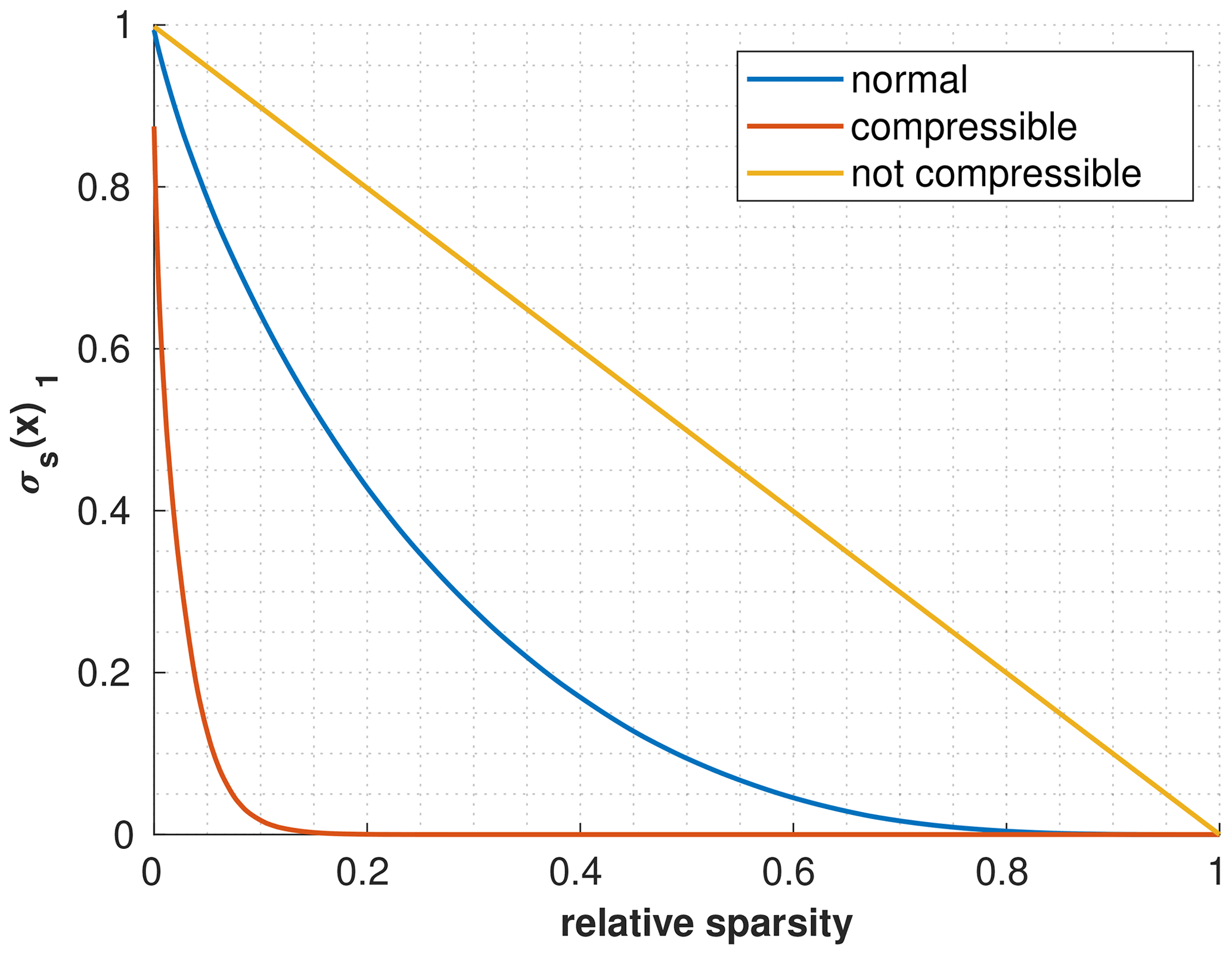
Figure 1Visualization of the compressibility of emission fields by plotting σs(x)1 over all s. The more hyperbolic the curve is, the more compressible the emission field.
An example is depicted in Fig. 1. The more hyperbolic the plot is, the more compressible the signal is. In order to get a measure for the compressibility of the distribution, the Gini index is used, which was also proposed as a sparsity measure for CS by Zonoobi et al. (2011). This index measures how unequally x is distributed, which is a similar measure to the hyperbolicity of a curve in the depicted figure. For the case of an equal distribution (yellow curve) the Gini index becomes 0, and for a highly compressible distribution (orange curve) the Gini index gets close to 1. A Gini index of exactly 1 is equal to a 1-sparse signal.
In this paper, a DWT is used to sparsify emissions, using Haar wavelets. Throughout the paper, we use the third-level wavelet transform and refer to its matrix as W and its inverse transformation as W−1. For an introduction to wavelets, we refer to Graps (1995) and Mallat (1999). For the visualization of a third-level DWT, see Fig. 1.1 in Mallat (1999).
The emission map x is transformed into its wavelet coefficients c by Wx=c and vice versa by . To transform the forward model Ax=y into the wavelet domain, we write
where is the new forward model. The wavelet coefficients are then determined by the modified Eq. (P1) problem.
Note that the CS conditions for are not the same as for A. Once the wavelet coefficients are determined, the emissions are estimated by .
2.6 Reconstruction algorithms
There have been many algorithms proposed for the task of CS and SR. However, our goal in this paper is not to compare these algorithms, instead, we want to demonstrate the applicability of SR in general for urban GHG emission assessments. We, therefore, only solve the initial SR problem, given in Eq. (P1). To find the minimum, we use the cvx library, a matlab package for specifying and solving convex programs (Grant and Boyd, 2014, 2008), using the gurobi optimizer as a backend (Gurobi Optimization, LLC, 2021).
For the noisy case, we solve a modified form of Eq. (P1), given by
where ϵ is the noise vector. This is equivalent to the Lasso with the right choice of λ. Since we generate the noise by design, the optimization process simplifies by choosing ϵ without having to find the right λ value.
We compare our results to regularized least squares, which we refer to as least squares (LSs) hereafter. The equation of the LS is given by
in the noiseless case. There, the solution is given by the pseudo-inverse. In the noisy case, the equation is given by
2.7 Data evaluation
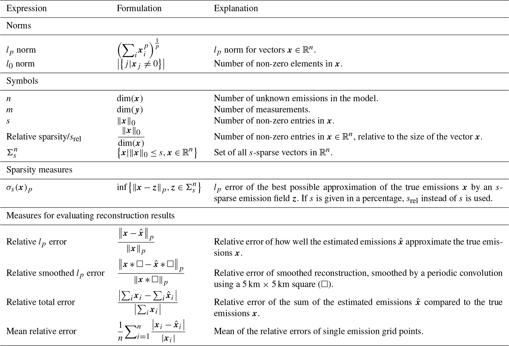
Table 1 gives an overview of the most important symbols and measures used in this paper. All of the measures we are using for evaluating the reconstruction results compare the estimations to the true emissions, which are the city emission inventories in this paper. If the lp error is not specified, the l2 error is used. The primary measure we use for the error evaluation of our estimates is the relative l2 error, since it provides a measure for the highest spatial resolution of the emissions (1 km × 1 km), while the relative l2 smoothed error shows an error for a lower spatial resolution (5 km × 5 km) and eliminates errors which are due to spatial errors. Because of the high spatial resolution of the emission fields reconstructed in this paper, relative l2 error values greater than 1 are possible. Those are because of spatial errors, where an emission is assigned to the wrong spatial location. The relative total error disregards these spatial errors and only evaluates the difference between the total estimated emission and the true total emission of a city.
The mean relative error is used if the relative error of emission grid points independent of their contribution to the total amount of emissions is of interest. This metric is useful to evaluate how well a reconstruction method estimates emitters of a certain kind.
Table 2Sparsity of the reported emission fields in different European cities. In the wavelet domain, in all of the cases a better or at least as good a sparse approximation of the emission map exists.
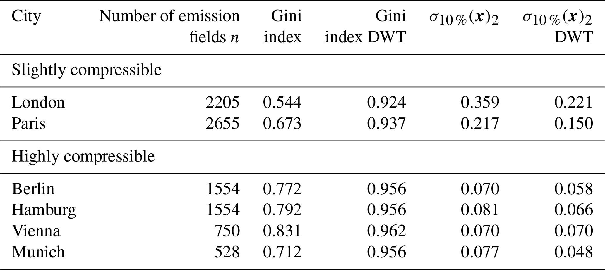
In the following, we determine the sparsity and compressibility of real-world emissions. To do so, we study the CO2 emissions of major European cities, such as Berlin, Hamburg, Munich, London, Paris, and Vienna using data from the TNO_GHGco_v1.1 emission inventory (van der Gon et al., 2019). This database provides annual gridded anthropogenic emissions with a resolution of about 1 km × 1 km for the areas and species. Furthermore, the emissions are classified by a proxy, such as public power, industry, and stationary combustion. Emissions of all proxies of the data set are included for the emission data used, making the assumption that this provides a good representation of typical emission fields for the cities investigated. We measure the sparsity of the cities using the Gini index and σ10 %(x)2 in the spatial and wavelet domain. The results are given in Table 2. For all the cities we consider, the wavelet domain of the emission fields achieves a higher Gini index compared to the spatial domain. Furthermore, the approximation error of srel=10 % of the signal is lower in the wavelet domain, except for Vienna, where this error is identical for both domains. From these data, we conclude that a representation of the city emission fields in the wavelet domain should generally be better suited for SR. We also split the cities into two groups: cities whose emission fields are highly compressible (Berlin, Hamburg, Vienna, and Munich; Gini index >0.7) and cities where the fields are significantly less compressible (London and Paris; Gini index <0.7).
In the following, we define the estimation problem (Sect. 4.1) and apply SR to several European cities (Sect. 4.2).
4.1 Formulating the estimation problem
In the following, we assume that the influence of the background GHG concentration on the measurements is fully known. Subtracting this influence from the measurements yields the enhancement produced by the GHG emissions in the domain of interest. Therefore, the background can be ignored, and the model is simplified to a pure transport emission system. Let the sensitivity of the GHG concentration measurements y to the city emissions x be given by the sensing matrix A:
The rows in A contain vectorized footprints, which determine the sensitivity of the measurements to the GHG fluxes of different emission grid cells in the domain. These footprints are determined by backward transport models, such as the Stochastic Time-Inverted Lagrangian Transport (STILT) model (Lin et al., 2003; Gerbig et al., 2003). In this paper, a simplified linear model, the Gaussian plume model, is used as the transport model. This approach allows varying parameters within the transport model without the computationally costly calculations of the STILT model. In Appendix B, we explain how the Gaussian plume footprints are created and show two footprints: one calculated by STILT, the other by the Gaussian plume model (Fig. B1). In our work, we use artificial wind data. These wind fields used, except in Sect. 4.2.1, possess a wind coverage of ∼143∘. All of the footprints generated by those wind fields are available at https://doi.org/10.5281/zenodo.5901298 (Zanger et al., 2022a).
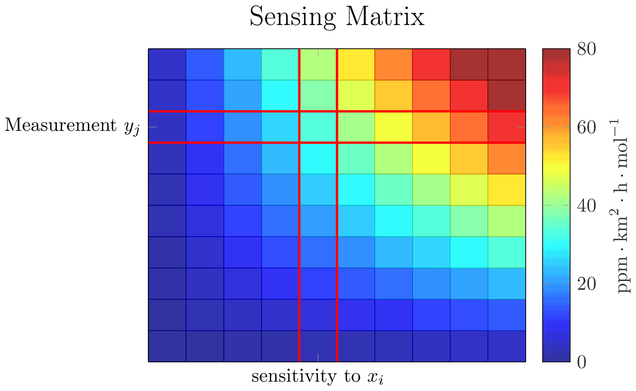
Figure 2Visualization of a sensing matrix, where the values in the matrix are color encoded. The entry Aji in the matrix gives the sensitivity of the jth measurement to the ith grid cell.
Figure 2 visualizes the sensing matrix A, which represents the sensitivity of all measurements to each grid cell. Depending on the footprints in A, there might be emissions in x which are not strongly sensed. The total sensitivity to a single grid cell xi is determined by the sum of the corresponding column in the sensing matrix. If this sensitivity is below a certain threshold, , where is the threshold, we remove the ith column from the sensing matrix and do not reconstruct this emission grid cell. For Fig. 2 this would be the first column of the sensing matrix, where all values are 0. This introduces some small perturbation between y and Ax, so that Ax≈y. However, since we choose our threshold small enough, this is not reflected in the solution but improves the conditioning of A and reduces the computational effort.
From a physical point of view, these removed emission grid cells are not situated upwind of the measurement stations and, therefore, cannot be well reconstructed using the measurements. For the wavelet domain, we perform this step on the wavelet transformed sensing matrix. Therefore, wavelet coefficients which are weakly sensed and below the threshold are removed.
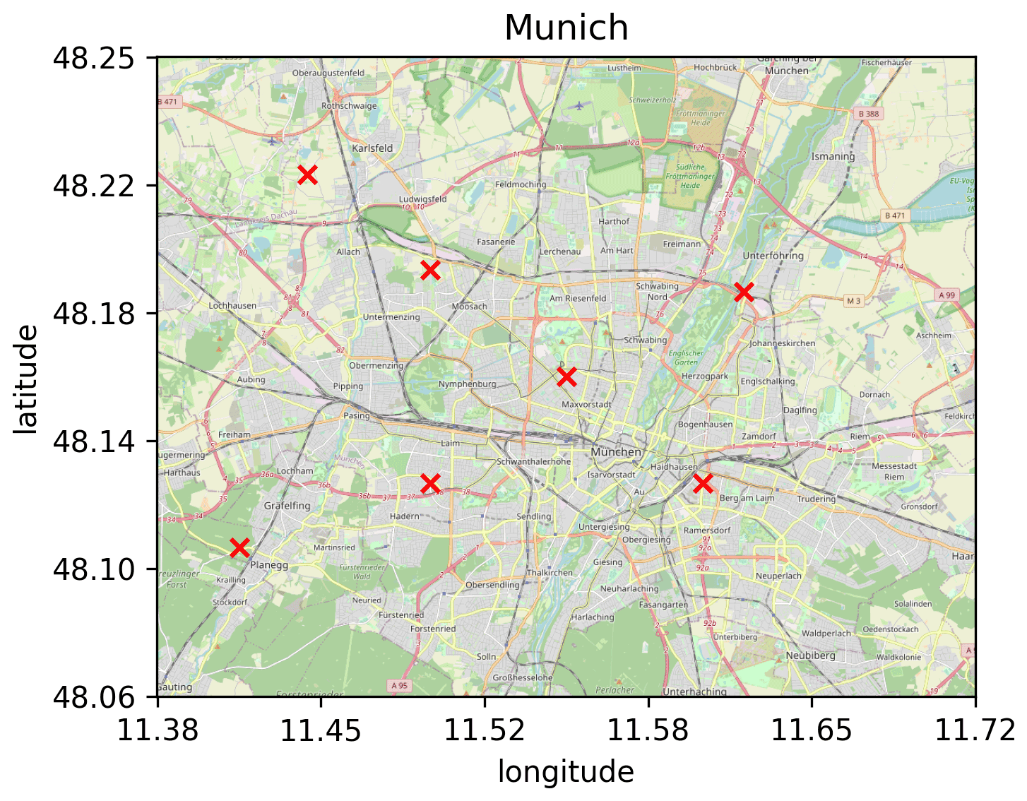
Figure 3Map of exemplary measurement locations for Munich using seven measurement stations, which represents a ratio of approximately 75 % (background: OpenStreetMap contributors, 2020).
In our study, we use both artificially created emission fields and real emission fields (van der Gon et al., 2019). Both field types have a spatial resolution of 1 km × 1 km. For the artificial emissions, a domain size of 32 km × 32 km is used, resulting in n=1024 unknown emission grids. For the emission inventory, the number of emission grids depends on the size of the city (see Table 2). In order to compare emission estimates of the different domains, we vary the number of measurement stations used for each domain, so that the number of measurements per unknown emission grid () is roughly constant. During the measurement period, each station takes 50 samples. The measurement stations were randomly distributed over a normalized area of the emission map and scaled to the domain size of each city. An exemplary distribution of the stations for Munich is depicted in Fig. 3, using %.
The measurements y are then created using the sensing matrix A and the emissions x: y=Ax. In the noisy case, we add a Gaussian distributed noise vector to the measurements: , . σϵ is chosen based on the SNR used.
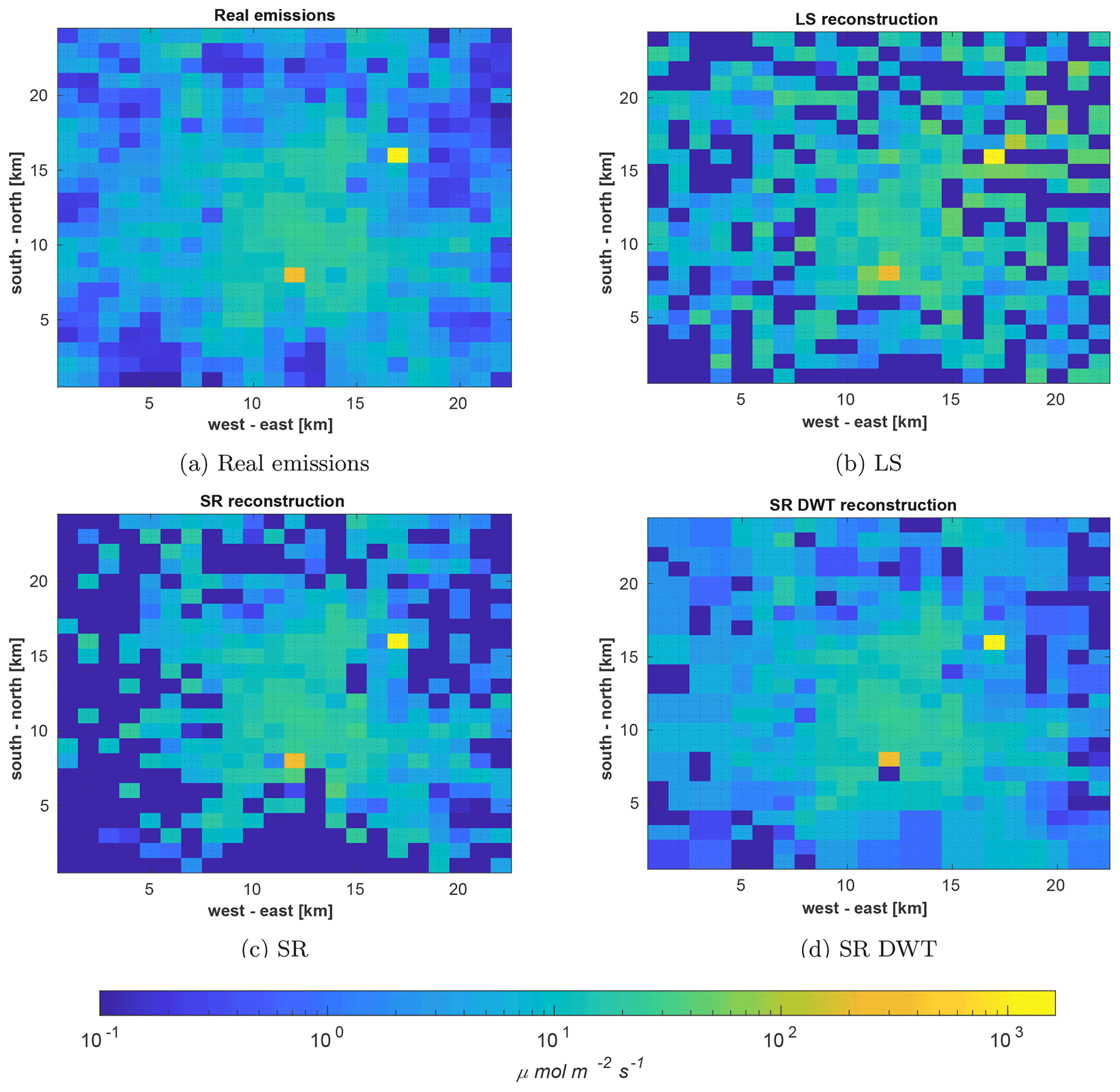
Figure 4Visualization of the (a) emission inventory of Munich and estimated emission fields of the inventory by using (b) LS, (c) SR, and (d) SR in the wavelet domain. The color scale is logarithmic and given in the unit of µmol (m2 s)−1. Negative emissions are colored dark blue and cannot be visually distinguished from low or 0 emitters. The emission inventory does not include negative emitters.
4.2 Applying sparse reconstruction to European cities
Reconstruction results for Munich in the noiseless case using LS, SR, and SR in the wavelet domain are depicted in Fig. 4, and the reconstruction errors for the figure can be found in Table 3. A visual inspection indicates that SR in the wavelet domain does resemble the real emissions best, while SR in the spatial domain is second best. Negative emitters are not visible because of the color scale. LS estimates a total of 171 such negative emitters with a total of 2139 µmol (m2 s)−1 negative emissions, while SR estimates only 33 negative emitters with a total of 9 µmol (m2 s)−1 negative emissions. SR in the wavelet domain estimates 50 negative emitters with a total of 59 µmol (m2 s)−1 negative emissions.
In the following, we identify properties of SR and compare them to the LS using the European city emission inventories. The properties we identify are interconnection between SR and CS (Sect. 4.2.1), the wavelet domain to make emissions sparser (Sect. 4.2.2), the ability of identifying unknown emitters (Sect. 4.2.3), and the number of measurements needed (Sect. 4.2.4). We first analyze these properties in the noiseless case (Sect. 4.2.1 to 4.2.4) and then extend those to the noisy case (Sect. 4.2.5).
Additionally, in Appendix A, we present an example using artificial, sparse emissions to better establish further connections between SR and CS.
4.2.1 Influence of wind coverage
We examine the effect of wind coverage on the effectiveness of the sensing matrix for SR. The term wind coverage is used to measure the range of wind directions during the measurement period. A wind coverage of 0∘ corresponds to no changes in the wind direction during the observations, while a wind coverage of 360∘ means that the wind blew from all directions during the time of observation.
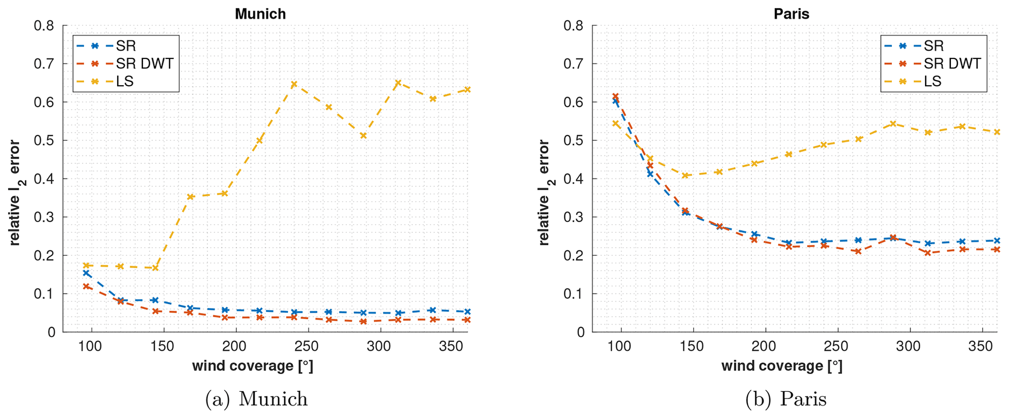
Figure 5Estimation errors for SR in the spatial and wavelet domain and LS reconstruction of (a) Munich's and (b) Paris's emissions with footprints covering different amount of wind directions. With a higher wind coverage, the estimation result using SR improves. The LS has no clear improvement for higher wind coverages, but its performance decreases with high coverages for Munich, while for Paris the performance first increases until about a coverage of 150∘ before decreasing again.
The wind coverage is changed in an interval from 96 to 360∘, with a step size of 24∘, using a Gaussian plume model. As emission field we use the CO2 city emission inventories of Munich and Paris from Sect. 3. Figure 5 depicts the relative errors of the SR in the spatial and wavelet domain and LS estimates of (a) Munich's and (b) Paris's emission fields. Errors of the estimates for both SR in the spatial and wavelet domain decrease with increasing wind coverage for Munich and Paris. In contrast, the LS estimates reveal no clear improvement for higher wind coverages, but the relative error of LS increases with high coverages for Munich, while for Paris the error initially decreases, until about a coverage of 150∘, before increasing again. A sensitivity analysis, given in Appendix F, reveals that error variations given by the different wind coverages are due to the shift in sensitivity to different parts of the domain, while the sum of the sensitivities does not change.
This major improvement in SR for higher wind coverage can be explained using the incoherence property from CS. The coherence parameter, given in Eq. (11), calculates the maximum similarity of how two emission grid cells are measured. For the spatial domain, by increasing the wind coverage, there is greater variety in the measurements and thus between the measurements of two different grid cells. In the wavelet domain, we determined the coherences at different wind coverages and found a similar behavior.
Even though for both domains the coherence for a wind coverage of 360∘ is too high to offer reconstruction guarantees, our example shows that including CS parameters in the design process can improve reconstruction results.
4.2.2 Sparse reconstruction in the wavelet domain
In the following, we compare reconstruction results of SR in the wavelet and spatial domains. Accordingly, s-sparse city emission fields are used to compare these domains. More precisely, the s highest emitters of the CO2 inventory of London are used to generate an s-sparse emission field. This allows us to determine at which trade-off in sparsity the wavelet domain can achieve better results compared to the spatial domain. We chose the inventory of London, since it has the emission field with the lowest compressibility (see Table 2).
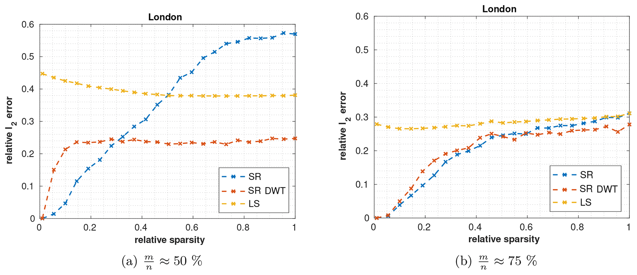
Figure 6Comparison of the LS (yellow) and SR in the spatial (blue) and wavelet (red) domains in terms of relative sparsity srel. An emission map artificially generated from London's emission inventory with a total of 2205 unknown emitters was used. The x axis represents the portion of these emitters that were used (the emitters are sorted from large to small). In (a) 22 measurement stations with a total of 1100 measurements and (b) 33 measurement stations with a total of 1650 measurements are used.
Figure 6 shows the relative reconstruction error in the spatial and third-level wavelet domain for different sparsity levels using % and %. As expected, SR in the spatial domain performs better for sparse emission maps (low s). For less sparse emission maps (higher s), however, the wavelet domain is superior.
With fewer measurements, the error in the wavelet domain already plateaus for srel≈15 %, while for % the error plateaus at srel≈40 %. The results also indicate that for the entire emission map of London (srel=1), the performance of SR in the wavelet domain does not increase significantly when the measurements are changed from to %, while the performance in the spatial domain benefits considerably. This improved performance is caused by the higher compressibility of the emission map in the wavelet domain, where the highest wavelet coefficients already provide a good representation of the entire emission map, while the spatial domain needs more coefficients for a representation with the same relative error. Therefore, the wavelet domain requires fewer measurements compared to the spatial domain, to achieve the same performance for cities with emission fields that have a low compressibility (for similar results see Sect. 4.3.3).
Our result demonstrates that the wavelet domain can help to improve SR in those instances for which the spatial domain is not well suited. However, changing the domain also alters the conditions of CS; therefore, conclusions made for CS in the spatial domain cannot be directly transferred to the wavelet domain.
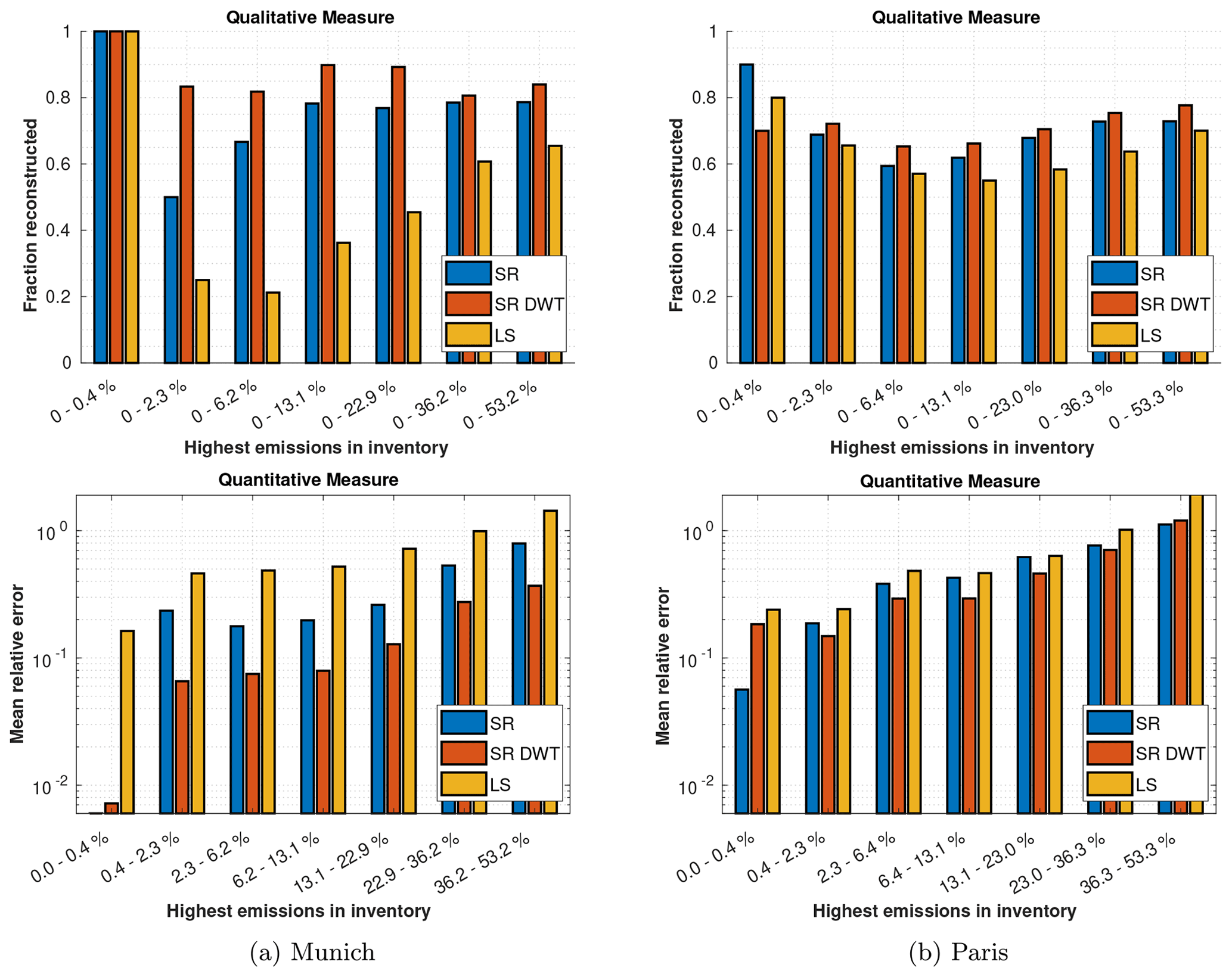
Figure 7Qualitative and quantitative measure of how well SR and LS estimate the highest emissions for (a) Munich and (b) Paris.
4.2.3 Discovering unknown emitters
In the following, we evaluate how well SR can identify unknown emitters. Assuming a good prior estimation of the emission field, where the relative error for the real emissions for each emitter is approximately constant and small, unknown emitters can be assumed to make a huge contribution to the difference between the prior expected measurements and real measurements. Therefore, we evaluate how well the highest emitters are reconstructed to assess the performance of finding unknown emitters.
To do this, we consider the emission inventory data for Munich and Paris. While Munich's emissions inventory is highly compressible, the emission inventory of Paris is not. For the setup, seven measurement stations are used in Munich and 39 in Paris. This results in % for both cities, making the estimation results comparable.
We employ a qualitative and a quantitative measure, both of which are depicted in Fig. 7. The x axes show bins of emission grids ranked by their emission strength. For example, the first bin (0 %–0.4 %) contains the first 0.4 % highest-emission grids, while the last bin in the lower panels of Fig. 7 contains emission grids which are among the 36.2 %–53.2 % highest-emission grids. Since the emissions have a high compressibility (the first highest emissions make a huge contribution to the total emissions), we use a logarithmic scale for the bins.
The qualitative measure (see upper panels in Fig. 7) compares the fraction of the highest emitters in the inventory matching those of the estimation (the higher the ratio, the better). In Munich, all three methods reconstruct the same largest 0.4 % emitters. For Paris, SR in the spatial domain performs best followed by the LS in the case of the largest 0.4 % emitters. For lower emitters, SR in the wavelet domain performs best for both cities. While the performance gain of SR and SR DWT over the LS method is quite large in Munich, which has a highly compressible emission inventory, the gain is smaller in Paris, which has a slightly compressible inventory.
The quantitative measure (see lower panels in Fig. 7) compares the relative error in the reconstructed emissions (the lower, the better). For the largest 0.4 % emitters, SR in the spatial domain performs best and can reconstruct these emissions with an error of less than 0.7 % in Munich and 3 % in Paris. When analyzing slightly lower emissions, SR in the spatial domain performance drops significantly and the wavelet domain performs best in both cities.
The results indicate that SR in the spatial domain works particularly well for the highest emitters (largest 0.4 % in our examples), while SR in the wavelet domain performs well for a broader range of high emitters. The LS performance is much less sensitive to the emission strength of individual strong emitters, which is not beneficial for estimating large unknown emitters.
These results for the same scenario but with fewer measurement stations ( %) can be found in Appendix D.
4.2.4 Number of measurements needed
Previous scenarios have presented comparisons between SR and LS using % or %. However, the question of how many measurements m are needed to produce results of a certain accuracy remains unanswered. To determine this, we vary the number of measurements per station, which leads to a variation in .
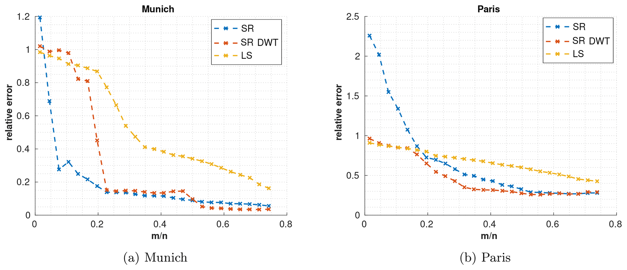
Figure 8Relative error for SR, SR with DWT, and LS at different degrees of undersampling, for (a) Munich and (b) Paris.
Figure 8 depicts the relative estimation error for Munich and Paris for varying . In Munich, where the emissions are highly compressible, the reconstruction error for SR in the spatial domain already drops sharply for %. SR in the wavelet domain needs more measurements but performs similar to the spatial domain using % and even performs slightly better than the spatial domain for %. The LS also sees a steep improvement with % but does not produce results as good as SR.
For Paris, where the emissions have a low compressibility, SR in the spatial domain performs worst for %, while the wavelet domain performs about the same as the LS for this number of measurements. For a higher number of measurements (), both SR methods show increased performance and both perform better than the LS. Overall, SR in the wavelet domain performs best.
These trends are also confirmed for the emissions of other cities (see Supplement). These results demonstrate that when using SR instead of the LS, a higher undersampling with fewer errors is possible, especially for highly compressible emissions (as in Munich).
4.2.5 Measurement noise
To make the results applicable to real-world scenarios, noise also has to be taken into consideration. There are different types of noise, including measurement noise, transport error, and representation error. In the following, we assume measurement errors with an SNR typical of column measurements. Chen et al. (2016) report measurement errors for column measurements for an average time of 10 min for CO2 as 0.04 to 0.05 ppm and for CH4 as 0.2 ppb. Jones et al. (2021) show that CH4 concentration enhancements measured for the city of Indianapolis are in the order of several parts per billion. Below, we assume an SNR of 20 dB, which corresponds to enhancements of 2 ppb for methane or 0.4 to 0.5 ppm for CO2.
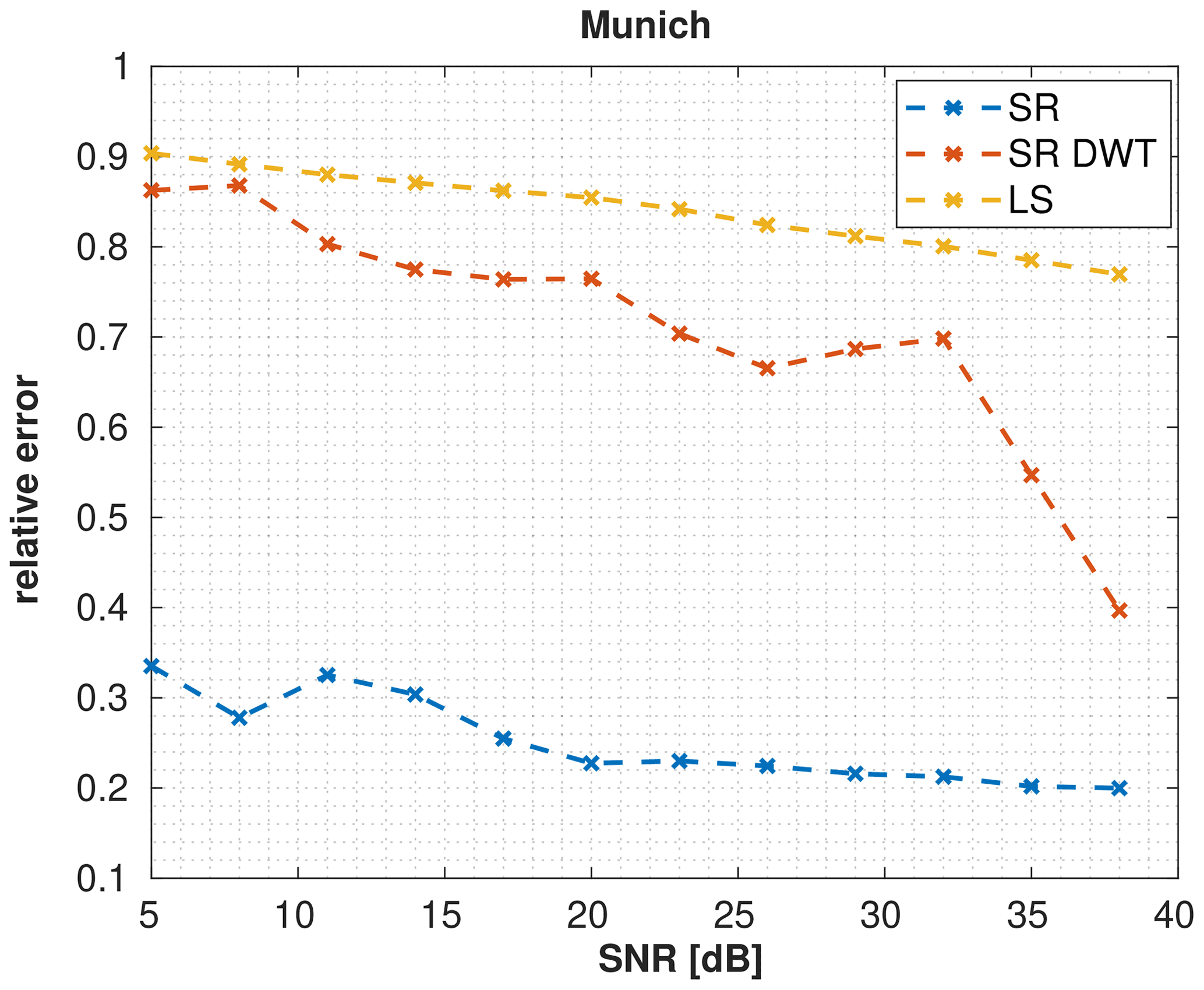
Figure 9Reconstruction errors of SR in the spatial and wavelet domain as well as LS for Munich when varying the SNR and .
As emission fields, we use the inventory data for Munich. Compared to the noiseless case, we increase the number of measurement stations to , which is 15 measurement stations with a total of 750 measurements. Figure 9 depicts how the relative l2 error changes for different SNRs in the Munich simulation. The figure shows that the results we obtain for an SNR of 20 dB should not differ significantly for slightly lower or higher SNRs between 15 and 25 dB. Therefore, we believe that despite our noise assumptions, which are optimistic compared to real-world scenarios, our results are qualitatively valid. We provide a variance map for SR with an SNR of 20 dB in Appendix E.
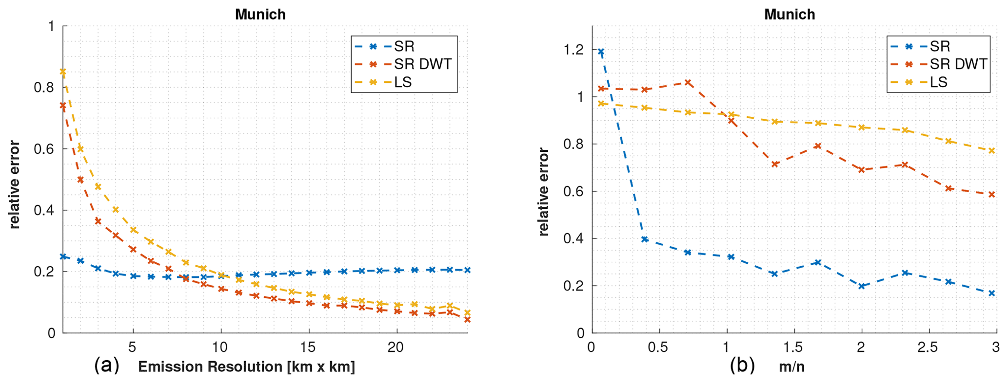
Figure 10Reconstruction errors use SR in the spatial and wavelet domain as well as the LS for Munich with an SNR of 20 dB, where (a) shows the average relative error for the reconstruction of 250 different noise vectors at different levels of resolutions using and (b) shows the relative error for the highest resolution (1 km × 1 km) when varying the number of measurements.
Here, we show the relative error of the estimated emission fields for the noisy case at different spatial resolutions of the emissions, both for SR in the spatial domain and wavelet domain and for the LS (see Fig. 10a). For this case we have run the reconstruction of 250 different noise vectors and show the mean estimation result. Furthermore, we assess the undersampling capability in the noisy case (see Fig. 10b). For SR in the spatial domain, the relative error is only slightly higher for high resolutions and remains fairly constant across other spatial resolutions, suggesting that almost all errors occur in the reconstruction of emission strength rather than in the localization of emitters. Both SR in the wavelet domain and the LS have a high relative error for high resolutions (below 7 km × 7 km), while at lower resolutions both perform better than SR in the spatial domain, indicating that most of the error is due to incorrect localization of emitters.
As a result, they do not provide accurate localization of the emitters. To overcome this, more measurements are needed for SR in the wavelet domain and LS. To determine the number of measurements required, we show the relative errors for the highest resolution (1 km × 1 km) when varying the number of measurements in Fig. 10b. For SR in the spatial domain, the relative error drops significantly for % and performs better than the other reconstruction methods for more measurements. The wavelet domain performs similarly to the LS for and better for . These results indicate that SR in the spatial domain, for Munich, is more robust against noise, while the wavelet domain is not as robust (many more measurements are needed than in the noiseless case for similar results).

Figure 11Qualitative and quantitative measure of how well SR and LS estimate the highest emissions with a noise of 20 dB for Munich. The qualitative plot shows how many percent of the highest emissions in the inventory are also contained in the same highest amount of emission of the reconstruction. The quantitative plot shows the mean relative errors for different emission strengths.
Next, we analyze the performance of finding unknown emitters in the noisy case. For this purpose, we use the same setup as in Sect. 4.2.3 but solely look at the emissions in Munich. We again use and add the noise with an SNR of 20 dB. We employ a qualitative and a quantitative measure, both of which are depicted in Fig. 11 (for the description of the measures, see Sect. 4.2.3). SR is the only method to identify the 0.4 % highest emitters (qualitative measure) and estimates their emissions with a significantly lower relative error of 2 % (quantitative measure). Slightly smaller emitters are better estimated by the SR in the wavelet domain. For even lower emitters, there is no clear winner of which method estimates them best. Compared to the noiseless case, the estimation errors are in general larger, and SR in the wavelet domain does not achieve as promising results as in the noiseless case. SR in the spatial domain remains sensitive to the largest emitters in the noisy case. These results for Paris can be found in the Supplement.
In the following, case studies on emission fields of all cities considered in Sect. 3 are introduced to more broadly compare the performance of SR. The measurement configuration corresponds to the specifications in Sect. 4.1. The emissions are reconstructed using SR in the spatial and wavelet domains as well as the LS, first with % in the noiseless case and then with in the noisy case.
Table 3Reconstruction performances for SR in the spatial and wavelet domain as well as for LS by measuring the relative error (1 km × 1 km), relative smoothed error (5 km × 5 km), and the relative total error for different European cities. The best approach for each city and type of error is highlighted in bold.

Table 4Reconstruction performances for SR in the spatial and wavelet domain as well as for LS by using with an SNR of 20.0 dB for different European cities. The results are evaluated using the relative error (1 km × 1 km), relative smoothed error (5 km × 5 km), and the relative total error. The best approach for each city and type of error is highlighted in bold.

To compare the performance, we measure relative errors, relative smoothed errors (for a spatial resolution of 5 km × 5 km), and relative total errors. The results for the noiseless case are in Table 3. At the highest spatial resolution (1 km × 1 km, right column in Table 3), SR performs much better than LS for the highly compressible emission fields in both domains. For the cities with emission fields that are slightly compressible, the SR performance is significantly worse than for the other cities but still slightly better than LS. For a lower spatial resolution of 5 km × 5 km (middle column in Table 3), the error of all methods decreases. Among the highly compressible emissions, SR still performs significantly better than LS. Both for London and Paris (slightly compressible), all methods produce a similar error, with the LS giving the smallest error in London and SR in the spatial domain giving the smallest error in Paris. For the total emissions, all reconstruction methods perform similarly.
These results support our previous findings that SR performs well at high resolutions for cities with highly compressible emissions.
Next, we consider the noisy case with an SNR of 20.0 dB and (see the results in Table 4).
For the cities that are slightly compressible, SR in the spatial domain performs the worst, while SR in the wavelet domain and the LS perform similarly.
For the highly compressible cities, SR in the spatial domain produces the best results for the 1 km × 1 km and 5 km × 5 km resolution and is worse than the other reconstruction methods for the total emissions (except for Vienna). Furthermore, SR in the wavelet domain performs better than the LS. In contrast to the noiseless case, SR in the wavelet domain performs worse than SR in the spatial domain for high resolutions (≲5 km × 5 km). Both results support our findings from Sect. 4.2.5 that SR in the spatial domain accurately localizes emissions and that SR in the wavelet domain is not as robust to noise as the spatial domain for high resolutions.
In this paper, we introduced sparse reconstruction (SR) as a novel method for the inversion of urban GHG emissions and further provided key examples to identify the advantages of SR to inversely model emissions.
SR can be easily integrated into existing top–down frameworks for estimating emission. We examined the applicability of this method by evaluating the sparseness of emissions from several European cities. Our results indicate that the emissions from most of these cities are sparse and that SR is applicable. We also showed that a wavelet transform increases the sparsity of urban emissions, making SR applicable to cities with less sparse emissions. SR is known to have reconstruction guarantees if conditions of compressed sensing (CS) are satisfied. We tested different CS conditions for various wind fields and showed that wind fields with better CS conditions do significantly increase the performance of SR.
Compared to state-of-the-art inversion methods using Gaussian priors, our method requires fewer measurements and provides better localization and quantification of unknown emitters.
SR works best if the underlying representation of the emissions is sparse. In this paper, we employed the wavelet transform to increase the sparsity; however, other transformations, such as a curvelet transform or more general dictionary representations, might be even more suited for specific spatial domains. Finding such transformations which also work well with CS conditions is challenging, and future studies should be devoted to them.
Table A1 shows the longitude and latitude boundaries used to create the CO2 emission fields for the European cities from the TNO_GHGco_v1.1 emission inventory.
Table A1Longitude and latitude boundaries used to create the CO2 emission inventories for the European cities from the TNO_GHGco_v1.1 emission inventory.

The sensing matrices we use consist of vectorized footprints generated by the Gaussian plume model with artificial wind data. The Gaussian plume model provides a good enough approximation for Lagrangian particle dispersion models for the purpose of this paper. The footprints are generated for a high-resolution grid using a dynamic Gaussian plume with varying wind speed, direction, and diffusion. The footprints are then scaled to the domain size of the city. Because of the scaling, the wind speed and diffusion changes for each city. Nevertheless, we think that this approach makes the reconstruction performances for different cities more comparable than using different footprints for every city.
For Sect. 4.2.1, we use a static Gaussian plume model to generate footprints for different wind coverages. This allows us to ignore additional effects from the dynamical case, for example, in the dynamic case the change in the wind direction produces spiral-looking footprints. These footprints have a different shape compared to the footprints generated using a static Gaussian plume model. By using a static model, the footprints are more predictable and systematic, which makes the results of different wind coverages more comparable to each other.
Figure B1 shows a comparison between a STILT footprint for Munich and a Gaussian plume footprint used in our work, where the two footprints are generated using different wind fields.
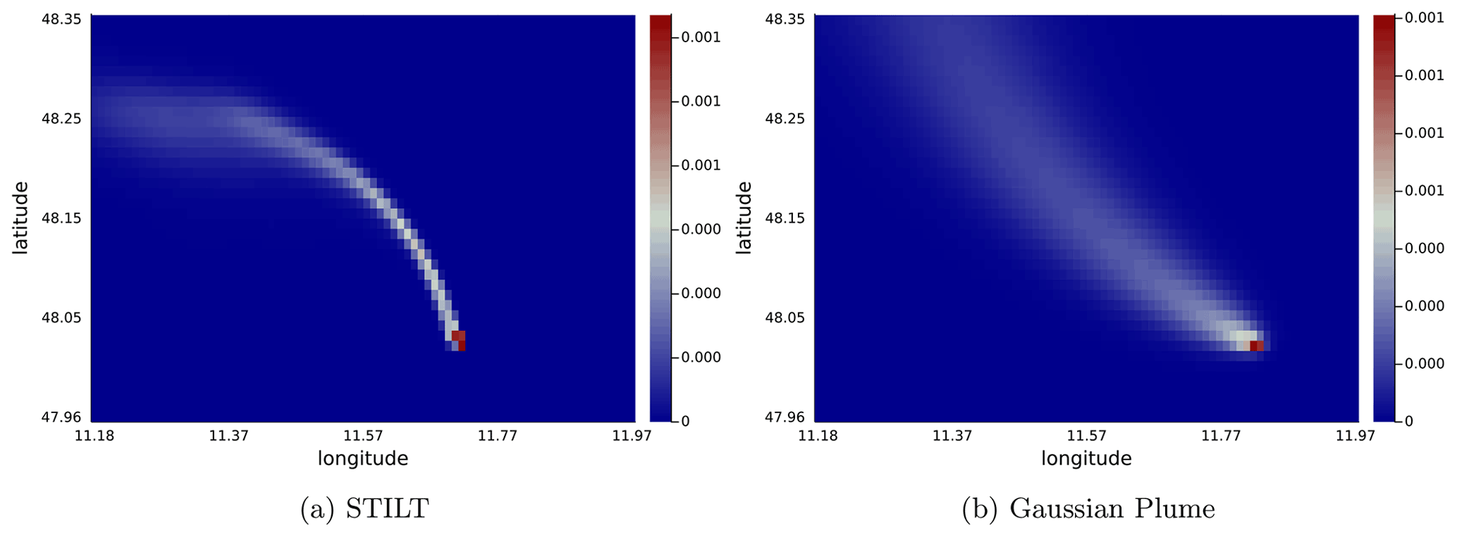
Figure B1Comparison of a STILT footprint to a Gaussian plume footprint, where different wind fields have been used.
Consider s emitters producing an s-sparse emission field in a city. We distribute these emitters over the city using a Gaussian distribution, such that the probability for an emitter in the center of the city is higher compared to outside of the city. Furthermore, we use a Gaussian distribution to model the emission strength of each emitter with a mean value of 10 µmol (m2 s)−1 and a standard deviation of 1 µmol (m2 s)−1, so that all emitters have roughly a similar contribution to the total emissions. In Fig. C1, the reconstruction errors for the spatial domain using SR and LS are depicted. SR allows exact recovery for srel≲13 % non-zero emissions using and for srel>35 % non-zero emissions using . In contrast, the relative error of LS is generally much higher but decreases with a larger number of measurements.
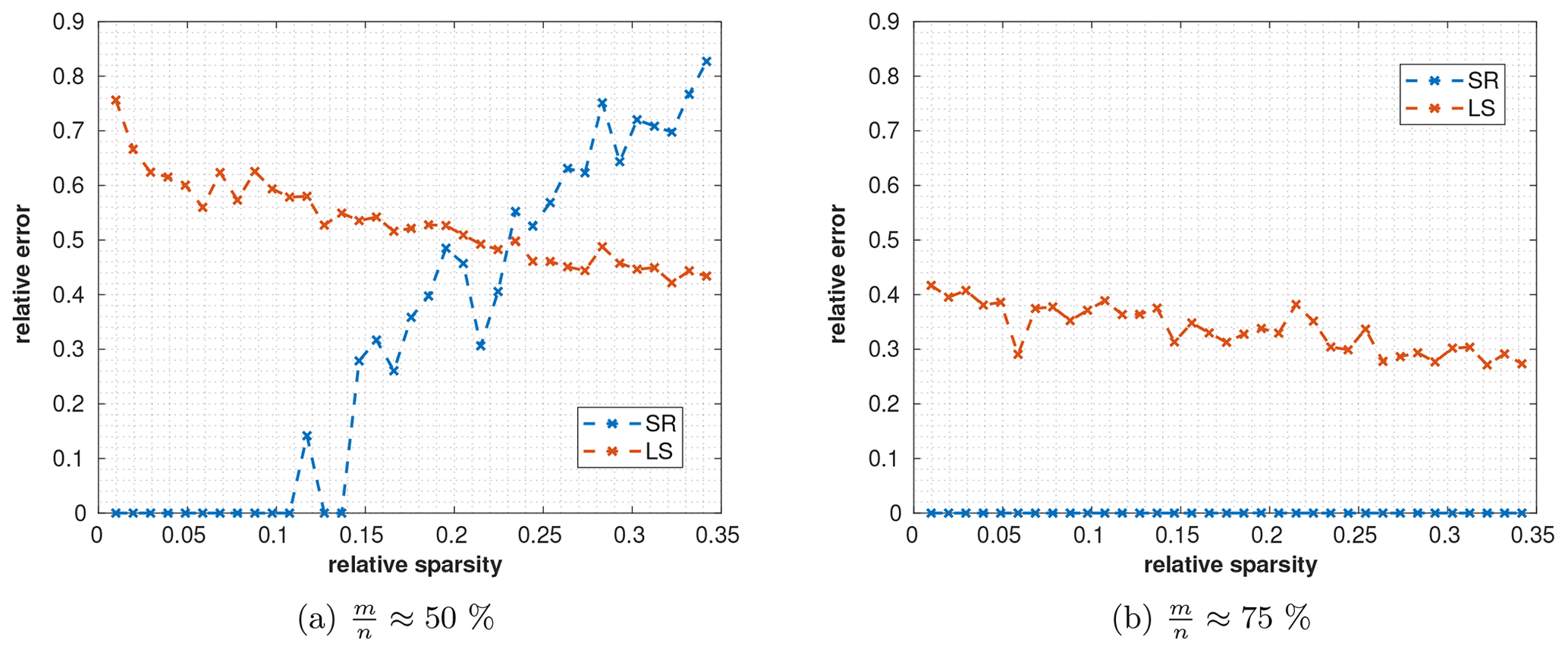
Figure C1Reconstruction errors for sparse cities with (a) 50 % and (b) 75 % measurements m per emission fields n. Using SR (blue line), it is possible to reconstruct sparse emissions. By increasing the number of measurement stations, and therefore observations, more emitters can be reconstructed using SR (a up to 13 %; b up to 35 % non-zero emission cells). For the LS method (red line), the relative error decreases both for less sparse signals and with a larger number of observations.

Figure C2Visualization of falsely discovered (dark blue), undiscovered (yellow), and discovered (cyan) emissions in x by (a) SR and (b) LS.
These results demonstrate the power of SR for sparse emission fields and illustrate the link between SR and CS. As shown in Sect. 2.4, the sensing matrix A must satisfy some sufficient conditions to ensure that CS yields the best possible reconstruction. However, in real-world scenarios, it is challenging to verify these conditions. By using a Monte Carlo algorithm, we found counterexamples that showed δ2s>1 for already small s (both for Gaussian plume footprints and STILT footprints). Thus, the sensing matrix we use here does not guarantee CS for all cases. Nevertheless, A can be useful if it satisfies the CS conditions for some specific emission distributions of interest.
Next, we consider the case with and choose a number of emitters s, such that the relative error produced by SR and the LS is similar.
Therefore, both methods produce the same relative error, which allows us to compare the spatial distribution of the error on an equal basis. This is the case for srel=46.9 %, where the relative error for SR is 28.1 %, while the relative error for LS is 27.3 %. We focus on the following questions:
-
which emitters are found correctly (discovered)?
-
which emitters are not found (undiscovered)?
-
which emitters are discovered, even though there is no emitter there (falsely discovered)?
Figure C2 depicts the discovered, not discovered, and falsely discovered emitters for SR (panel a) and LS (panel b). SR reconstructs most emitters correctly, only 1.1 % of the emitters are undiscovered (yellow), and 8.0 % are falsely discovered (dark blue). In contrast, the LS has no emitters which have not been found but 45.6 % falsely discovered emitters. This is because the LS prefers smooth estimates, which is equivalent to estimating emitters everywhere. This is also seen by the fraction between the emissions estimated for falsely discovered emitters and the total estimated emissions. While this fractions is only 3.0 % for SR, for LS this fraction is 12.2 %.
These results demonstrates the advantage of SR for the localization of emitters. This property is especially useful to find unknown emitters, since the spatial certainty of emitters for SR is much higher.
In Sect. 4.2.3 we showed that SR is better at finding high emitters compared to LS and can reconstruct them with smaller errors. This is visualized by Fig. 7, which has been created using . In the following, we visualize this result using only .
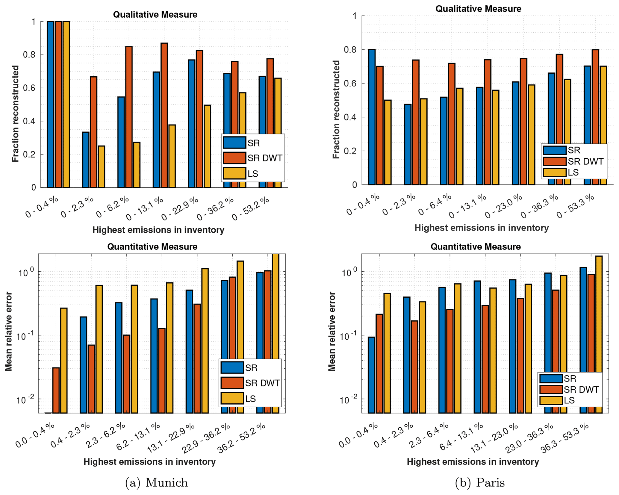
Figure D1Qualitative and quantitative measure of how well SR and LS estimate the highest emitters for Munich (a) and Paris (b) using .
The results are depicted in Fig. D1. Compared to the case with more measurements, for Munich, SR in the spatial domain performs better in the qualitative measure compared to the wavelet domain. Furthermore, for Paris, the margin between the performance of SR in the wavelet domain and the other methods has increased.
Uncertainty quantification for sparse reconstruction is distinctly different compared to uncertainty quantification for LS reconstruction. First, while for the LS fit with Gaussian noise a closed-form solution exists, there does not exist any closed-form solution for sparse reconstruction.
In the following we use the uncertainty quantification approach from Hase et al. (2017) in order to derive a variance plot of the reconstruction result by applying bootstrapping. This gives us the covariance matrices for SR in the spatial and wavelet domain. We only use the variances of the matrix and plot the standard deviations for every single reconstructed emission, which is depicted in Fig. E1. For the spatial domain, the standard deviation is localized around certain areas in the map, while for the wavelet domain, the standard deviation covers much larger areas of the map. This lets one believe that a reconstructed emission in the spatial domain has a higher certainty of location compared to SR in the wavelet domain. This assumption is verified by Fig. 10.
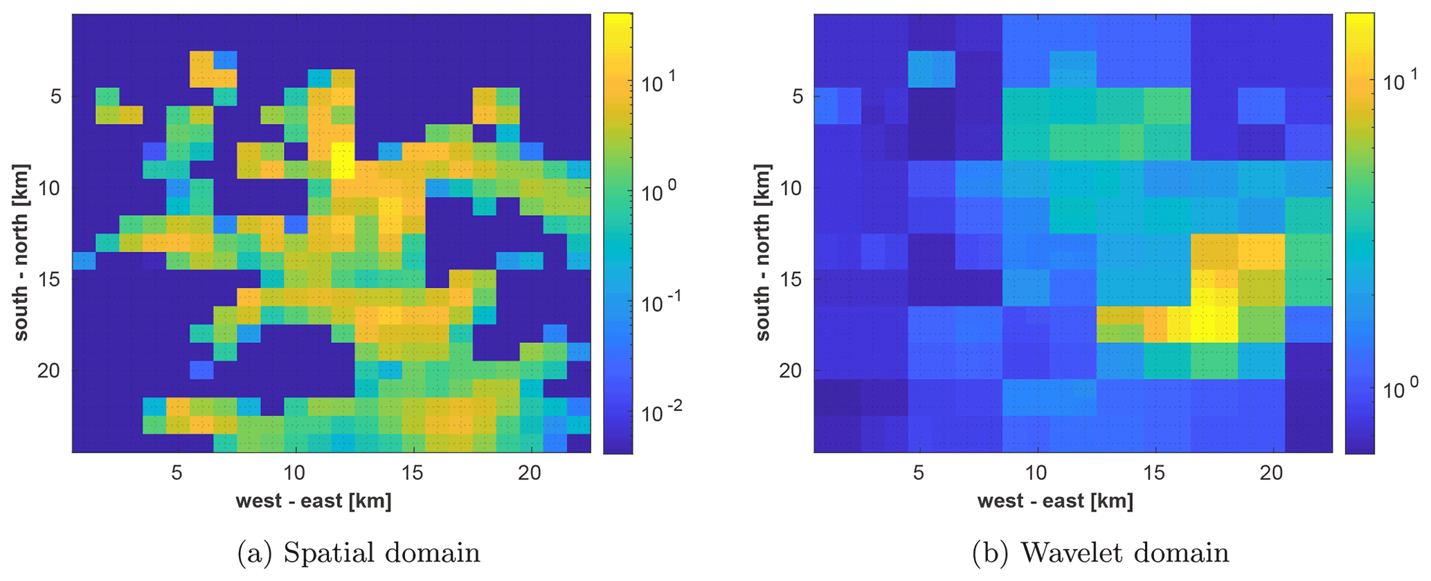
Figure E1Uncertainty of the emission estimates for Munich with and an SNR of 20 dB for SR in the (a) spatial domain and (b) wavelet domain.
In the following, we show that the changes in relative error for LS in Sect. 4.2.1 are due to the fact that the sensitivity to different areas of the map changes, while the total sensitivity does not change. Figure F1 depicts the sensitivity map of Munich for a wind coverage of (a) 72∘ and (b) 360∘. For 72∘, the southeast has good sensitivity to the estimation, while other parts, especially the west of the city, are weakly sensitive. For 360∘, there is no area in the city which is not sensitive to the estimation. However, some areas are less sensitive than in the 72∘ case, especially the southeast. If we compare this sensitivity map to the emission map of Munich in Fig. 4, we see that the strongest emitter is positioned in the southeast. This explains why, for the case of 72∘, the relative error of the LS is lower than for the 360∘ case. If we look at the mean sensitivity of an emission grid cell for both cases, we find that those are exactly the same (0.6629), and a change in wind coverage does not improve the total sensitivity.
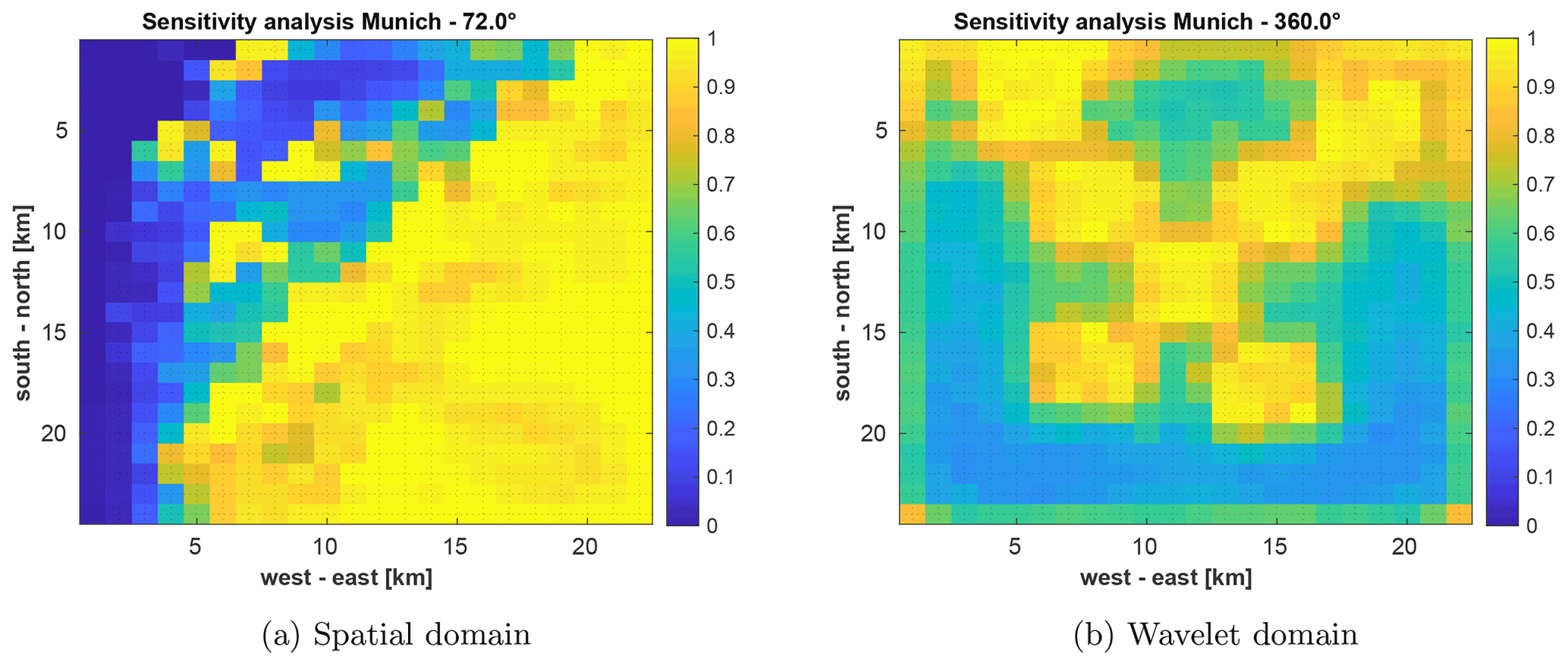
Figure F1Sensitivity map of LS in Munich for a wind coverage of (a) 72∘ and (b) 360∘. In (a), the southeast has good sensitivity to the estimation, while the west and north of the city are only weakly sensitive. In (b), there is no area which is not sensitive to the estimation, but the areas in the southeast are less sensitive.
The code for this paper is written in Matlab 2021a and available on Zenodo: https://doi.org/10.5281/zenodo.6757562 (Zanger et al., 2022b). The Gaussian plume footprints are available at https://doi.org/10.5281/zenodo.5901298 (Zanger et al., 2022a). The TNO_GHGco_v1.1 emission inventory (van der Gon et al., 2019) is not publicly available. The latitude and longitude boundaries used to generate the city emission fields from the inventory are given in Appendix A.
The supplement related to this article is available online at: https://doi.org/10.5194/gmd-15-7533-2022-supplement.
JC and FD conceived the study. BZ and MS performed the data analysis supervised by JC and FD. BZ, JC, and FD wrote the paper. BZ and JC revised the paper according to the reviewer comments. MS contributed to the content of the paper. JC acquired the funding and guided the project.
The contact author has declared that none of the authors has any competing interests.
Publisher's note: Copernicus Publications remains neutral with regard to jurisdictional claims in published maps and institutional affiliations.
We would like to thank Alihan Kaplan from the chair of Theoretical Information Technology for his comments and useful discussions. We would also like to thank Stephen Starck for helping us to improve the language of the paper. We are thankful to the editor and the reviewers for their valuable comments and suggestions, which helped to improve the paper. Benjamin Zanger, Jia Chen, and Florian Dietrich were supported by the Deutsche Forschungsgemeinschaft (DFG, German Research Foundation) (grant nos. CH 1792/2-1 and INST 95/1544).
This research has been supported by the Deutsche Forschungsgemeinschaft (grant nos. CH 1792/2-1 and INST 95/1544).
This work was supported by the German Research Foundation (DFG) and the Technical University of Munich (TUM) in the framework of the Open Access Publishing Program.
This paper was edited by Jinkyu Hong and reviewed by Scot Miller and two anonymous referees.
Baraniuk, R., Davenport, M., DeVore, R., and Wakin, M.: A simple proof of the restricted isometry property for random matrices, Constructive Approximation, 28, 253–263, https://doi.org/10.1007/s00365-007-9003-x, 2008. a
Boche, H., Calderbank, R., Kutyniok, G., and Vybíral, J.: A survey of compressed sensing, in: Compressed sensing and its applications, 1–39, Springer, 2015. a
Candès, E. J.: The restricted isometry property and its implications for compressed sensing, Comptes Rendus Mathematique, 346, 589–592, https://doi.org/10.1016/j.crma.2008.03.014, 2008. a, b
Candès, E. J. and Tao, T.: Decoding by linear programming, IEEE T. Inform. Theory, 51, 4203–4215, https://doi.org/10.1109/TIT.2005.858979, 2005. a
Candès, E. J., Romberg, J. K., and Tao, T.: Stable signal recovery from incomplete and inaccurate measurements, Commun. Pure Appl. Math., 59, 1207–1223, https://doi.org/10.1002/cpa.20124, 2006. a
Candès, E. J., Eldar, Y. C., Needell, D., and Randall, P.: Compressed sensing with coherent and redundant dictionaries, Appl. Comput. Harmon. A., 31, 59–73, https://doi.org/10.1016/j.acha.2010.10.002, 2011. a
Chen, J., Viatte, C., Hedelius, J. K., Jones, T., Franklin, J. E., Parker, H., Gottlieb, E. W., Wennberg, P. O., Dubey, M. K., and Wofsy, S. C.: Differential column measurements using compact solar-tracking spectrometers, Atmos. Chem. Phys., 16, 8479–8498, https://doi.org/10.5194/acp-16-8479-2016, 2016. a, b
Dietrich, F., Chen, J., Voggenreiter, B., Aigner, P., Nachtigall, N., and Reger, B.: MUCCnet: Munich Urban Carbon Column network, Atmos. Meas. Tech., 14, 1111–1126, https://doi.org/10.5194/amt-14-1111-2021, 2021. a
Gerbig, C., Lin, J. C., Wofsy, S. C., Daube, B. C., Andrews, A. E., Stephens, B. B., Bakwin, P. S., and Grainger, C. A.: Toward constraining regional-scale fluxes of CO2 with atmospheric observations over a continent: 2. Analysis of COBRA data using a receptor-oriented framework, J. Geophys. Res.-Atmos., 108, 4757, https://doi.org/10.1029/2003JD003770, 2003. a
Göckede, M., Turner, D. P., Michalak, A. M., Vickers, D., and Law, B. E.: Sensitivity of a subregional scale atmospheric inverse CO2 modeling framework to boundary conditions, J. Geophys. Res.-Atmos., 115, D24112, 2010. a
Golub, G. H., Hansen, P. C., and O'Leary, D. P.: Tikhonov regularization and total least squares, SIAM J. Matrix Anal. A., 21, 185–194, 1999. a
Grant, M. C. and Boyd, S. P.: Graph Implementations for Nonsmooth Convex Programs, in: Recent Advances in Learning and Control, edited by: Blondel, V. D., Boyd, S. P., and Kimura, H., Lecture Notes in Control and Information Sciences, 371, Springer, London, https://doi.org/10.1007/978-1-84800-155-8_7, 2008. a
Grant, M. and Boyd, S.: CVX: Matlab Software for Disciplined Convex Programming, version 2.1, http://cvxr.com/cvx (last access: 28 September 2022), 2014. a
Graps, A.: An introduction to wavelets, IEEE Comput. Sci. Eng., 2, 50–61, 1995. a
Gurobi Optimization, LLC: Gurobi Optimizer Reference Manual, https://www.gurobi.com (last access: 28 September 2022), 2021. a
Hase, F., Frey, M., Blumenstock, T., Groß, J., Kiel, M., Kohlhepp, R., Mengistu Tsidu, G., Schäfer, K., Sha, M. K., and Orphal, J.: Application of portable FTIR spectrometers for detecting greenhouse gas emissions of the major city Berlin, Atmos. Meas. Tech., 8, 3059–3068, https://doi.org/10.5194/amt-8-3059-2015, 2015. a
Hase, N., Miller, S. M., Maaß, P., Notholt, J., Palm, M., and Warneke, T.: Atmospheric inverse modeling via sparse reconstruction, Geosci. Model Dev., 10, 3695–3713, https://doi.org/10.5194/gmd-10-3695-2017, 2017. a, b, c
Hirsch, A. I., Michalak, A. M., Bruhwiler, L. M., Peters, W., Dlugokencky, E. J., and Tans, P. P.: Inverse modeling estimates of the global nitrous oxide surface flux from 1998–2001, Global Biogeochem. Cycles, 20, GB1008, https://doi.org/10.1029/2004GB002443, 2006. a
Hong, M., Yu, Y., Wang, H., Liu, F., and Crozier, S.: Compressed sensing MRI with singular value decomposition-based sparsity basis, Phys. Med. Biol., 56, 6311–6325, https://doi.org/10.1088/0031-9155/56/19/010, 2011. a
Jacob, D. J., Turner, A. J., Maasakkers, J. D., Sheng, J., Sun, K., Liu, X., Chance, K., Aben, I., McKeever, J., and Frankenberg, C.: Satellite observations of atmospheric methane and their value for quantifying methane emissions, Atmos. Chem. Phys., 16, 14371–14396, https://doi.org/10.5194/acp-16-14371-2016, 2016. a
Jones, T. S., Franklin, J. E., Chen, J., Dietrich, F., Hajny, K. D., Paetzold, J. C., Wenzel, A., Gately, C., Gottlieb, E., Parker, H., Dubey, M., Hase, F., Shepson, P. B., Mielke, L. H., and Wofsy, S. C.: Assessing urban methane emissions using column-observing portable Fourier transform infrared (FTIR) spectrometers and a novel Bayesian inversion framework, Atmos. Chem. Phys., 21, 13131–13147, https://doi.org/10.5194/acp-21-13131-2021, 2021. a, b, c, d, e
Klappenbach, F., Chen, J., Wenzel, A., Forstmaier, A., Dietrich, F., Zhao, X., Jones, T., Franklin, J., Wofsy, S., Frey, M., Hase, F., Hedelius, J., Wennberg, P., Cohen, R., and Fischer, M.: Methane emission estimate using ground based remote sensing in complex terrain, EGU General Assembly 2021, online, 19–30 Apr 2021, EGU21-15406, https://doi.org/10.5194/egusphere-egu21-15406, 2021. a
Lewis, A. S. and Knowles, G.: Image compression using the 2-D wavelet transform, IEEE T. Image Proc., 1, 244–250, 1992. a
Lin, J. C., Gerbig, C., Wofsy, S. C., Andrews, A. E., Daube, B. C., Davis, K. J., and Grainger, C. A.: A near-field tool for simulating the upstream influence of atmospheric observations: The Stochastic Time-Inverted Lagrangian Transport (STILT) model, J. Geophys. Res.-Atmos., 108, 4493, https://doi.org/10.1029/2002JD003161, 2003. a
Mallat, S.: A Wavelet Tour of Signal Processing, Elsevier, https://doi.org/10.1016/b978-0-12-466606-1.x5000-4, 1999. a, b
Miller, S. M., Wofsy, S. C., Michalak, A. M., Kort, E. A., Andrews, A. E., Biraud, S. C., Dlugokencky, E. J., Eluszkiewicz, J., Fischer, M. L., Janssens-Maenhout, G., Miller, B. R., Miller, J. B., Montzka, S. A., Nehrkorn, T., and Sweeney, C.: Anthropogenic emissions of methane in the United States, P. Natl. Acad. Sci. USA, 110, 20018–20022, https://doi.org/10.1073/pnas.1314392110, 2013. a
Mueller, K. L., Gourdji, S. M., and Michalak, A. M.: Global monthly averaged CO2 fluxes recovered using a geostatistical inverse modeling approach: 1. Results using atmospheric measurements, J. Geophys. Res.-Atmos., 113, D21114, https://doi.org/10.1029/2007JD009734, 2008. a
Nakamura, G. and Potthast, R.: Inverse modeling, IOP Publishing, ISBN 978-0-7503-1218-9, https://doi.org/10.1088/978-0-7503-1218-9, 2015. a
OpenStreetMap contributors 2020. Distributed under the Open Data Commons Open Database License (ODbL) v1.0.: Map data, distributed under the Open Data Commons Open Database License (ODbL) v1.0, https://www.openstreetmap.org/copyright (last access: 28 September 2022), 2020. a
Ray, J., Yadav, V., Michalak, A. M., van Bloemen Waanders, B., and McKenna, S. A.: A multiresolution spatial parameterization for the estimation of fossil-fuel carbon dioxide emissions via atmospheric inversions, Geosci. Model Dev., 7, 1901–1918, https://doi.org/10.5194/gmd-7-1901-2014, 2014. a, b
Ray, J., Lee, J., Yadav, V., Lefantzi, S., Michalak, A. M., and van Bloemen Waanders, B.: A sparse reconstruction method for the estimation of multi-resolution emission fields via atmospheric inversion, Geosci. Model Dev., 8, 1259–1273, https://doi.org/10.5194/gmd-8-1259-2015, 2015. a, b, c, d
Sargent, M., Barrera, Y., Nehrkorn, T., Hutyra, L. R., Gately, C. K., Jones, T., McKain, K., Sweeney, C., Hegarty, J., Hardiman, B., Wang, J. A., and Wofsy, S. C.: Anthropogenic and biogenic CO2 fluxes in the Boston urban region, P. Natl. Acad. Sci. USA, 115, 7491–7496, https://doi.org/10.1073/pnas.1803715115, 2018. a
Shekhar, A., Chen, J., Paetzold, J. C., Dietrich, F., Zhao, X., Bhattacharjee, S., Ruisinger, V., and Wofsy, S. C.: Anthropogenic CO2 emissions assessment of Nile Delta using XCO2 and SIF data from OCO-2 satellite, Environ. Res. Lett., 15, 095010, https://doi.org/10.1088/1748-9326/ab9cfe, 2020. a
Shusterman, A. A., Teige, V. E., Turner, A. J., Newman, C., Kim, J., and Cohen, R. C.: The BErkeley Atmospheric CO2 Observation Network: initial evaluation, Atmos. Chem. Phys., 16, 13449–13463, https://doi.org/10.5194/acp-16-13449-2016, 2016. a
Su, W., Bogdan, M., and Candès, E.: FALSE DISCOVERIES OCCUR EARLY ON THE LASSO PATH, Ann. Stat., 45, 2133–2150, 2017. a
Tibshirani, R.: Regression Shrinkage and Selection via the Lasso, J. Roy. Stat. Soc. B, 58, 267–288, 1996. a
Tillmann, A. M. and Pfetsch, M. E.: The Computational Complexity of the Restricted Isometry Property, the Nullspace Property, and Related Concepts in Compressed Sensing, IEEE T. Inform. Theory, 60, 1248–1259, https://doi.org/10.1109/TIT.2013.2290112, 2014. a
Toja-Silva, F., Chen, J., Hachinger, S., and Hase, F.: CFD simulation of CO2 dispersion from urban thermal power plant: Analysis of turbulent Schmidt number and comparison with Gaussian plume model and measurements, J. Wind Eng. Ind. Aerod., 169, 177–193, https://doi.org/10.1016/j.jweia.2017.07.015, 2017. a
Turner, A. J., Jacob, D. J., Wecht, K. J., Maasakkers, J. D., Lundgren, E., Andrews, A. E., Biraud, S. C., Boesch, H., Bowman, K. W., Deutscher, N. M., Dubey, M. K., Griffith, D. W. T., Hase, F., Kuze, A., Notholt, J., Ohyama, H., Parker, R., Payne, V. H., Sussmann, R., Sweeney, C., Velazco, V. A., Warneke, T., Wennberg, P. O., and Wunch, D.: Estimating global and North American methane emissions with high spatial resolution using GOSAT satellite data, Atmos. Chem. Phys., 15, 7049–7069, https://doi.org/10.5194/acp-15-7049-2015, 2015. a
Turner, A. J., Kim, J., Fitzmaurice, H., Newman, C., Worthington, K., Chan, K., Wooldridge, P. J., Köehler, P., Frankenberg, C., and Cohen, R. C.: Observed Impacts of COVID-19 on Urban CO2 Emissions, Geophys. Res. Lett., 47, e2020GL090037, https://doi.org/10.1029/2020GL090037, 2020. a
van der Gon, H. D., Kuenen, J., Boleti, E., Muntean, M., Maenhout, G., Marshall, J., and Haussaire, J.-M.: Emissions and natural fluxes Dataset, https://www.che-project.eu/sites/default/files/2019-01/CHE-D2-3-V1-0.pdf (last access: 28 September 2022), 2019. a, b, c
Viatte, C., Lauvaux, T., Hedelius, J. K., Parker, H., Chen, J., Jones, T., Franklin, J. E., Deng, A. J., Gaudet, B., Verhulst, K., Duren, R., Wunch, D., Roehl, C., Dubey, M. K., Wofsy, S., and Wennberg, P. O.: Methane emissions from dairies in the Los Angeles Basin, Atmos. Chem. Phys., 17, 7509–7528, https://doi.org/10.5194/acp-17-7509-2017, 2017. a
Wang, Y., Zeng, J., Peng, Z., Chang, X., and Xu, Z.: Linear convergence of adaptively iterative thresholding algorithms for compressed sensing, IEEE T. Signal Process., 63, 2957–2971, 2015. a
Wesloh, D., Lauvaux, T., and Davis, K. J.: Development of a Mesoscale Inversion System for Estimating Continental-Scale CO2 Fluxes, J. Adv. Model. Earth Sy., 12, e2019MS001818, https://doi.org/10.1029/2019MS001818, 2020. a, b
Yan, S., Wu, C., Dai, W., Ghanem, M., and Guo, Y.: Environmental Monitoring via Compressive Sensing, in: Proceedings of the Sixth International Workshop on Knowledge Discovery from Sensor Data, SensorKDD '12, p. 61–68, Association for Computing Machinery, New York, NY, USA, https://doi.org/10.1145/2350182.2350189, 2012. a
Zanger, B., Chen, J., Sun, M., and Dietrich, F.: Gaussian plume footprints, Zenodo [data set], https://doi.org/10.5281/zenodo.5901298, 2022a. a, b
Zanger, B., Chen, J., Sun, M., and Dietrich, F.: tum-esm/recovery_of_sparse_urban_greeenhouse_gas_emissions: v0.1.0, Zenodo [code], https://doi.org/10.5281/zenodo.6757562, 2022b. a
Zonoobi, D., Kassim, A. A., and Venkatesh, Y. V.: Gini Index as Sparsity Measure for Signal Reconstruction from Compressive Samples, IEEE J. Sel. Top. Sig., 5, 927–932, https://doi.org/10.1109/JSTSP.2011.2160711, 2011. a
- Abstract
- Introduction
- Methodology
- The sparsity/compressibility of emissions in European cities
- Evaluating sparse reconstruction of GHG emissions
- Broader comparison of sparse reconstruction for European cities
- Conclusions
- Appendix A: Boundaries of the emission inventories
- Appendix B: Wind fields and generation of the sensing matrix
- Appendix C: Recovery of sparse emissions
- Appendix D: Discovering unknown emitters using fewer measurements
- Appendix E: Uncertainty quantification
- Appendix F: Least square sensitivity for different wind coverages
- Code and data availability
- Author contributions
- Competing interests
- Disclaimer
- Acknowledgements
- Financial support
- Review statement
- References
- Supplement