Repeatable high-resolution statistical downscaling through deep learning

One of the major obstacles for designing solutions against the imminent climate crisis is the scarcity of high spatio-temporal resolution model projections for variables such as precipitation. This kind of information is crucial for impact studies in fields like hydrology, agronomy, ecology, and risk management. The currently highest spatial resolution datasets on a daily scale for projected conditions fail to represent complex local variability. We used deep-learning-based statistical downscaling methods to obtain daily 1 km resolution gridded data for precipitation in the Eastern Ore Mountains in Saxony, Germany. We built upon the well-established climate4R framework, while adding modifications to its base-code, and introducing skip connections-based deep learning architectures, such as U-Net and U-Net++. We also aimed to address the known general reproducibility issues by creating a containerized environment with multi-GPU (graphic processing unit) and TensorFlow's deterministic operations support. The perfect prognosis approach was applied using the ERA5 reanalysis and the ReKIS (Regional Climate Information System for Saxony, Saxony-Anhalt, and Thuringia) dataset. The results were validated with the robust VALUE framework. The introduced architectures show a clear performance improvement when compared to previous statistical downscaling benchmarks. The best performing architecture had a small increase in total number of parameters, in contrast with the benchmark, and a training time of less than 6 min with one NVIDIA A-100 GPU. Characteristics of the deep learning models configurations that promote their suitability for this specific task were identified, tested, and argued. Full model repeatability was achieved employing the same physical GPU, which is key to build trust in deep learning applications. The EURO-CORDEX dataset is meant to be coupled with the trained models to generate a high-resolution ensemble, which can serve as input to multi-purpose impact models.

1 Introduction

The Earth has undoubtedly warmed at an alarming rate in recent decades (IPCC, 2021), with the last one, 2011–2020, being the warmest on record. The last 7 years (2015–2021) have been the warmest on record as well, while 2020, tied with 2016, was the hottest (WMO, 2022). Notably, during 2020 the Pacific Ocean entered a La Niña phase, which conveys an overall cooling effect, in contrast to the El Niño warming conditions observed in 2016 (Voosen, 2021), which can be seen as a strengthening of the warming trend by man-induced climate change. The above mentioned facts are based on global averages. On a smaller scale, there have been several signs of the effects that climate change can have on extreme events, e.g. the 2020 fires in Siberia, California, and Australia; the 2021 summer flash floods events in western Europe and China; and the 2021 summer heat waves on the Northern Hemisphere soon after observing the coldest April in Germany for decades.

Climate change is one of the greatest challenges faced by humankind and general circulation models (GCMs) are the best tools available to model the response of the climate system to different forcing scenarios. Nevertheless, despite the remarkable improvements of GCMs over recent years, their spatial resolution yields their outputs unfit to be used directly for regional climate change impact studies in fields such as hydrology, agronomy, ecology, and risk management (Maraun and Widmann, 2018). The resolution of GCMs can be of up to a few hundred kilometres, depending on the GCM generation, which results in large regional biases when contrasted to station data (Flato et al., 2013). To overcome this hindrance, downscaling methodologies are employed, which transform coarse GCM output to regional- and local-scale (von Storch et al., 1993).

Dynamical downscaling uses the initial and boundary conditions from GCM output to drive high-resolution regional climate models (RCMs) (Hallett, 2002). The Coordinated Regional Climate Downscaling Experiment (CORDEX, 2021) offers multiple RCM output variables at daily temporal resolution based on CMIP5 (Taylor et al., 2012) projections with a spatial resolution of 0.44, 0.22, and 0.11^∘ (approximately 50, 25, and 12.5 km, correspondingly), with the highest resolution being available only for Europe. Regardless, these great efforts and the improved performance against the 0.44^∘ models (Pastén-Zapata et al., 2020), the resolution still does not meet the needs of impact modellers, which can be a few kilometres or less, particularly for topographically complex regions.

Statistical downscaling methods build empirical relationships or transfer functions between the larger-scale atmospheric variables (predictors) and regional- or local-scale variables (predictands) (Hewitson and Crane, 1996; Maraun and Widmann, 2018), such as precipitation or temperature. Perfect prognosis is the particular statistical downscaling methodology used in the present study, which requires a daily correspondence between predictors and predictands. Statistical downscaling implementations have significantly evolved since the 1990s through technological advances, with increasing amounts of input data, performance, complexity, and computational demands. Consequently, several methods have been studied for statistical downscaling, e.g. linear models for station data (paired with canonical correlation analysis, von Storch et al., 1993); artificial neural networks (ANNs, Hewitson and Crane, 1996; Wilby and Wigley, 1997; Cavazos and Hewitson, 2005); support vector machines (Tripathi et al., 2006; Pour et al., 2016); random forest (He et al., 2016; Pang et al., 2017); and, recently, modern ANNs architectures and deep learning techniques for gridded data (Vandal et al., 2018; Baño-Medina et al., 2020; Höhlein et al., 2020; Serifi et al., 2021).

Baño-Medina et al. (2020) provided a comparison between several deep learning models and more classical methods, such as generalized linear models, while validating the results with a robust framework such as VALUE (Maraun et al., 2014; Gutiérrez et al., 2019). Baño-Medina et al. (2020) also introduced the downscaleR.keras R package, which enables the use of the Keras (Chollet et al., 2015) and TensorFlow (Abadi et al., 2015) machine learning libraries in climate4R (Iturbide et al., 2019). Even though deep learning methods were examined in the aforementioned paper, the applied models do not exploit modern convolutional neural networks (CNNs) architectures, like skip or residual connection-based models (Srivastava et al., 2015) such as U-Net (Ronneberger et al., 2015) and U-Net++ (Zhou et al., 2018), which allow state-of-the-art performance in computer vision assignments. Additionally, since the study was developed for the whole of Europe with intercomparison purposes, the target resolution of the statistical downscaling method is too coarse (0.5^∘) for impact studies.

Furthermore, reproducibility is at the core of good scientific practices, yet it is a challenging feature to achieve in several scientific areas. Stoddart (2016) states that from a poll of 1500 scientists, more than 70 % of researchers were not able to reproduce another scientist's experiment and more than half were unsuccessful reproducing their own experiments. Reproducibility especially is a known issue for climate modelling (Bush et al., 2020) and also for calculations carried out on GPU (graphic processing unit) systems (Jézéquel et al., 2015; Nagarajan et al., 2018; Alahmari et al., 2020), particularly when applying machine learning frameworks that do not guarantee determinism.

Reproducibility is a term that is not standardized in the scientific literature. Depending on the source, field, and circumstances, repeatability and replicability are employed (Rougier et al., 2017; Nagarajan et al., 2018; Association for Computing Machinery (ACM), 2021), which undoubtedly leads to confusion. The ACM adopted the three terms based upon the definition in the International Vocabulary of Metrology (Joint Committee for Guides in Metrology, 2006) for conditions of a measurement. Under the ACM terminology, repeatability implies the same measurement precision by the same team and the same experimental setup. This is the only condition achievable within any singular publication, since the other two involve another independent team. Despite their conflicting definitions respectively focused on computer science and deterministic deep learning, both Rougier et al. (2017) and Nagarajan et al. (2018) allowed discrepancies between observations if the results are qualitatively the same or equivalent, which can be particularly relevant for deep learning applications. Additionally, Goodman et al. (2016) proposed methods reproducibility, results reproducibility, and inferential reproducibility to address this nomenclature confusion. Analogously, only methods reproducibility is achievable within any publication and this implies to provide “enough detail about study procedures and data so the same procedures could, in theory or in actuality, be exactly repeated” (Goodman et al., 2016).

Due to its less conflictive definition and what is achievable within a publication, repeatability will be pursued hereafter. Still, general reproducibility will be employed for broader use of the terminology. The concept of “qualitatively the same” or “equivalent” results will be referred to as similarity, to avoid consensus with conflicting definitions. Also, we aspire to comply with the methods reproducibility condition of Goodman et al. (2016). For a more comprehensive overview on the general reproducibility-related terminology, the reader is referred to Plesser (2018).

TensorFlow is the deep learning framework employed in the downscaleR.keras R package and in climate4R. To our knowledge, there is limited scientific literature on the repeatability capacities of TensorFlow on GPU systems. Nagarajan et al. (2018) dealt with the sources of non-determinism for both PyTorch and TensorFlow deep learning frameworks, but could not achieve determinism with the latter, and therefore neither repeatability. Alahmari et al. (2020) were able to use the deterministic implementations of some TensorFlow algorithms with versions 1.14 and 2.1, yet could only achieve repeatability with v2.1 using the LeNet-5 model but not with an U-Net. Nevertheless, newer versions of TensorFlow have included further deterministic implementations of GPU algorithms (NVIDIA, 2021).

The aim of this paper is to apply the statistical downscaling methodology for precipitation in the Eastern Ore Mountains, employing as predictors the ERA5 reanalysis (Hersbach et al., 2020) and as predictands the ReKIS (Regional Climate Information System for Saxony, Saxony-Anhalt, and Thuringia) dataset, generated at the Chair of Meteorology of the Technische Universität Dresden (Kronenberg and Bernhofer, 2015) in order to develop and validate transfer functions under modern deep learning architectures. These transfer functions can be subsequently used to downscale a climate projection ensemble directly from dynamically downscaled data (e.g. CORDEX model output), rather than from GCMs, as in Quesada-Chacón et al. (2020), to a suitable scale for multi-purpose climate change impact models. The rationale of building on top of the climate4R framework in a containerized environment is to ease and verify its repeatability, an imperative which we intend to deepen, shed light upon, and standardize for further research.

This paper is structured as follows: Sect. 2 presents details of the datasets employed as predictors and predictands. In Sect. 3, we describe the downscaling methodology, the models used to create the transfer functions, the tools employed to evaluate the models, the hardware and software used, and the experimental workflow to assess the repeatability. The Sect. 4 presents the results and discussion related to the performance of the models and to the general reproducibility of the results. Lastly, Sect. 5 renders a summary of the investigation, its conclusions, and further research outlook.

2 Data

2.1 Focus region

The Ore Mountains, as the study area of the present paper, is a transnational mountain range that acts as a natural border between Germany and the Czech Republic. It is a region with rich mining history and multiple resources. On the German side, the range is part of the Ore Mountains/Vogtland Nature Park, established in 1990 with an area of 1495 km², of which 9 % corresponds to settlements, 30 % to agriculture, and 61 % to forests. The highest points on the German side are the Fichtelberg (elevation 1215 m) and the Kahleberg (elevation 905 m) in the Eastern Ore Mountains. The Ore Mountains contain five biotopes that provide invaluable ecosystem services to the region. Particularly, the Eastern Ore Mountains are characterized by the species-rich mountain meadows biotope, which offers recreation, wildlife observation chances, distinctive scenery, and herbs for medical purposes (Bastian et al., 2017). The Eastern Ore Mountains are the present focus region (see Fig. 1a).

Figure 1 Location of the study region and the predictor's domain. (a) Relative bias (RB) of precipitation between training and validation periods for the whole ReKIS domain for Saxony. The study region, Eastern Ore Mountains, abbreviated as EOM in the figure, is inside the darker grey line. (b) Topography of Germany, the centre of the ERA5 sub-domain pixels (marked by dots, 32 by 32) used for the predictors and the Eastern Ore Mountains.

2.2 Predictands

A subset of the ReKIS (2021) gridded dataset for the Free State of Saxony was used as predictand, which has a spatial resolution of 1 km at a daily temporal resolution. This dataset uses station data from the German Meteorological Service (Deutscher Wetterdienst, DWD) and the Czech Hydrometeorological Institute (CHMI) as source (Kronenberg and Bernhofer, 2015). There are several variables available from this dataset, nevertheless the present paper focuses on precipitation.

The raw station data for precipitation were corrected after Richter (1995) and interpolated using indicator kriging (Deutsch and Journel, 1998) for the probabilities of precipitation. Ordinary kriging (Wackernagel, 2010) with a negative weight correction and exponential semivariogram model according to Deutsch (1996) was employed to estimate the amounts of precipitation. The gridded dataset ranges from 1961 until 2015. The original ReKIS dataset for Saxony (shown in Fig. 1a) was cropped to the Eastern Ore Mountains region, giving a region with 1916 pixels to be modelled.

2.3 Predictors

The reanalysis dataset employed as predictors is ERA5 (Hersbach et al., 2020), which has a spatial resolution of 0.25^∘, 137 model levels interpolated to pressure levels, and hourly temporal resolution. In this study, the dataset from 1979 onwards was employed to train the transfer functions. The atmospheric variables used, as in Baño-Medina et al. (2020), are zonal and meridional wind, temperature, geopotential, and specific humidity at the 1000, 850, 700, and 500 hPa levels, for a grand total of 20 different variables. The ERA5 dataset was aggregated to daily resolution and was 32 pixels (8 by 8^∘) domain size, centred over the Eastern Ore Mountains as displayed in Fig. 1b.

3 Methods

3.1 Statistical downscaling

As previously mentioned, we built on top of the climate4R framework, particularly on the code made available by Baño-Medina et al. (2020), since it provides a great number of tools and the robust validation framework VALUE (Maraun et al., 2014; Gutiérrez et al., 2019). The code needed to recalculate the results to be presented can be found on Zenodo (Quesada-Chacón, 2022a), with all the modifications and extensions derived for our approach.

Statistical downscaling methods create a relationship between the predictors x and the predictands y by a statistical model F(.) or transfer function (Maraun and Widmann, 2018). Under the perfect prognosis approach, the calibration of the transfer functions is performed with “perfect” reanalysis predictors x_ERA5 characterized by temporal correspondence with the observed data y_ReKIS. The variables chosen (see Sect. 2.3) have shown a high predictive power for Europe (Baño-Medina et al., 2020).

The period from 1979 to 2009 was used to train the transfer functions and the one between 2010 and 2015 as hold-out validation dataset. The reason for this training–validation split lies in the interest of evaluating the performance of the transfer functions under extrapolation conditions, since there has been a change in the precipitation regime between both time periods. This change tends to on average drier conditions in the training period, as observed in Fig. 1a, where the relative bias is calculated as $({\stackrel{\mathrm{‾}}{\mathrm{Pr}}}_{\mathrm{Train}}-{\stackrel{\mathrm{‾}}{\mathrm{Pr}}}_{\mathrm{Val}})/{\stackrel{\mathrm{‾}}{\mathrm{Pr}}}_{\mathrm{Train}}$ with ${\stackrel{\mathrm{‾}}{\mathrm{Pr}}}_{\mathrm{Train}}$ and ${\stackrel{\mathrm{‾}}{\mathrm{Pr}}}_{\mathrm{Val}}$ the averaged daily precipitation of training and validation period, respectively. Notably, the latter might be significantly influenced by the 2013 summer floods, where the Eastern Ore Mountains was a focal point of heavy precipitation within Saxony. Also, the dataset does not include observations from 2015 until today, including the period from 2018–2019 where a long-lasting drought was observed (Mühr et al., 2018).

3.2 Transfer functions

Baño-Medina et al. (2020) demonstrated that deep learning architectures improved the performance of the transfer functions when compared to “classic” models (linear and generalized linear models), attributable to the capacity of the CNNs to learn from the spatial distribution and patterns of the input layers. Particularly, the CNN1 architecture was the best overall for precipitation. Its topology consists of three layers of CNNs, with 50, 25, and 1 filters or feature channels, respectively, which in terms of state-of-the-art deep learning is a rather simple architecture. Therefore, there is room for improvement for the transfer functions under more recent architectures, such as U-Net (Ronneberger et al., 2015), which was developed for biomedical image segmentation implementing skip connections, and U-Net++ (Zhou et al., 2018). The latter is an iteration of the U-Net with improved skip connections between layers, translating usually to a better performance (Harder et al., 2020). Both architectures introduce a contraction path, also known as encoder, and a symmetric expansion path, the decoder (see Fig. 2).

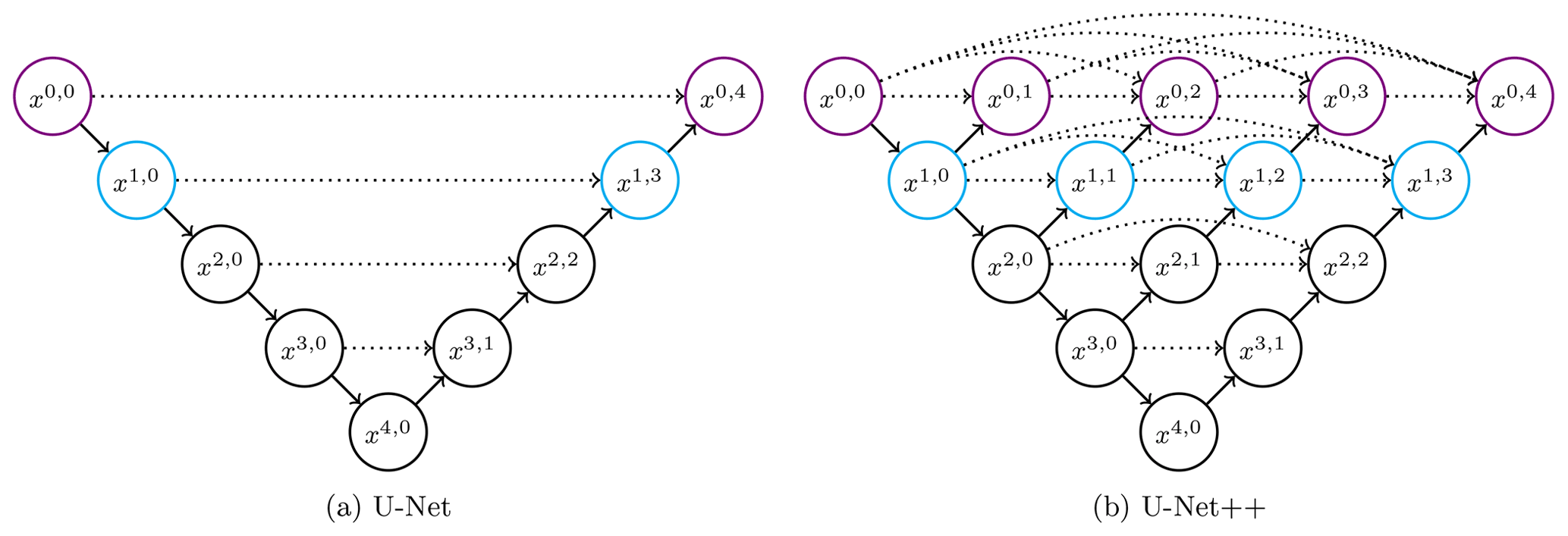
Figure 2 Skip connection-based models tested for the transfer functions. The three-layer version of each model is made up of only the black coloured nodes, the four-layer version of the black plus the cyan nodes, and the five-layer version of all of them. The ↘ represents down-sampling, the ↗ up-sampling, and the skip connections. The nodes x^i,j represent the ConvBlocks.

The encoder path reduces the spatial data contained in the input layers while increasing the feature information. The expansion path decodes the features obtained from the previous steps to match the target domain size. The skip connections provide access to the intermediate information contained in the features of the previous layers while smoothing the loss landscape (Li et al., 2018), which in turn speeds up the training process.

The depth of the skip connections-based architectures was a variable to optimize. Therefore, both architectures were tested under a three-, four-, and five-layers arrangement. Several numbers of starting feature channels were tested. The basic “convolutional unit” (ConvUnit) consisted of a convolutional layer (kernel size 3 by 3), with the respective activation function, and optional batch normalization and spatial drop-out. The last two options are used to avoid overfitting of the model. Batch normalization standardizes the layer's input data, which also improves learning speed, while spatial drop-out (2D version of Keras) randomly ignores entire feature maps during training. Two successive ConvUnits constitute a “convolutional block” hereafter referred to as ConvBlock.

On the contraction paths, for each node a ConvBlock was applied, followed by a max pooling layer (2 by 2 pool size) or down-sampling. All the previous layers used the padding = "same" setting of Keras. On the decoder path, a transposed convolutional layer was employed, halving the number of channels of the previous layer with a kernel size of 2 by 2 (up-sampling). Subsequently, all the respective skip connections for each node are concatenated and then another ConvBlock is applied to the resulting concatenation.

After processing all the respective nodes and layers, a single ConvUnit with a 1 by 1 kernel size and no spatial drop-out is applied. Several combinations of activation functions and feature channels were tested for this last ConvUnit. Then, as in Baño-Medina et al. (2020), the target function to optimize is the Bernoulli Gamma probability distribution function $f(y;\mathit{\rho },\mathit{\alpha },\mathit{\beta })$ (Cannon, 2008, see Eq. 1), and here especially the negative log-likelihood of it (Eq. 2). The probability of rain occurrence ρ, and the distribution parameters α (shape) and β (scale) were computed for each pixel. All of the tested combinations of skip connection-based models were then compared to the best-performing architecture from Baño-Medina et al. (2020), CNN1. Also other models similar to CNN1 were added for examination i.e. CNN32-1 consisting of three CNNs layers of 32, 16, and 1 filters; CNN64-1 comprising four CNNs with 64, 32, 16, and 1 channels; and lastly, CNN64_3-1 with 64, 32, and 1 features.

$$\begin{array}{}\text{(1)}& {\displaystyle }f(y;\mathit{\rho },\mathit{\alpha },\mathit{\beta })& {\displaystyle }=\left\{\begin{array}{ll}\mathrm{1}-\mathit{\rho }& \text{if}y=\mathrm{0}\\ {\displaystyle \frac{\mathit{\rho }\cdot (y/\mathit{\beta }{)}^{\mathit{\alpha }-\mathrm{1}}\cdot e^{-y/\mathit{\beta }}}{\mathit{\beta }\cdot \mathrm{\Gamma }\left(\mathit{\alpha }\right)}}& \text{if}y>\mathrm{0}\end{array}\right.\text{(2)}& {\displaystyle }-\ln f& {\displaystyle }=\left\{\begin{array}{ll}-\ln (\mathrm{1}-\mathit{\rho })& \text{if}y=\mathrm{0}\\ {\displaystyle \frac{\mathit{\alpha }\cdot \ln \mathit{\beta }+\ln \mathrm{\Gamma }\left(\mathit{\alpha }\right)+y/\mathit{\beta }}{\ln \mathit{\rho }+(\mathit{\alpha }-\mathrm{1})\cdot \ln y}}& \text{if}y>\mathrm{0}\end{array}\right.\end{array}$$

Several activation functions were tested, e.g. Sigmoid, ReLu (Xu et al., 2015), Leaky ReLu (α=0.3, see Eq. 3) and a linear function. Spatial drop-out ratios of 0, 0.25, and 0.5 were also examined. The optimizer used is Adam (Kingma and Ba, 2015), for which different learning rates were explored. The patience for the early stopping criteria was also a variable. In addition, several batch sizes were employed according to the available memory of the graphic processing units (GPUs). Throughout the calibration process of the models, 90 % of the data were randomly selected for training and the remaining 10 % were used for during-training validation.

$$\begin{array}{}\text{(3)}& \text{Leaky ReLu}\left(x\right)=\left\{\begin{array}{ll}x& \text{if}x>\mathrm{0}\\ \mathit{\alpha }\cdot x& \text{otherwise}\end{array}\right.\end{array}$$

3.3 Model evaluation

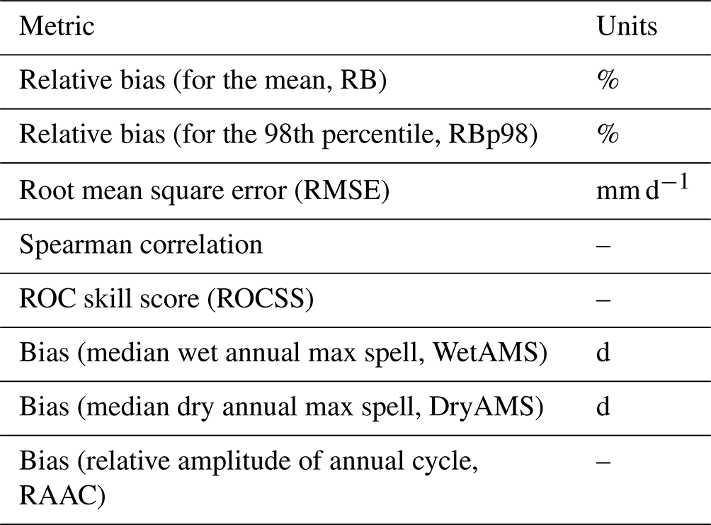
In order to work under comparable conditions, the metrics employed in the present study correspond to the ones used by Baño-Medina et al. (2020) included in the VALUE framework (Maraun et al., 2014; Gutiérrez et al., 2019), which allows to validate numerous aspects such as extremes and the spatio-temporal structure. Among these metrics are the relative bias, for both the mean and the 98th percentile, calculated both under deterministic and stochastic approaches; the root mean square error (RMSE); the temporal Spearman correlation; the relative operating characteristic (ROC) skill score (Manzanas et al., 2014); the bias of the median wet (WetAMS) and dry (DryAMS) annual max spells; and the bias of the relative amplitude of the annual cycle, using a 30 d moving window. A summary of the metrics is shown in Table 1, alongside their units.

Table 1 Metrics selected from VALUE to validate the performance of the transfer functions.

3.4 Hardware

The models were trained on the Alpha Centauri sub-cluster of the Center for Information Services and High Performance Computing (ZIH) of the Technische Universität Dresden, which consists of 34 nodes, each one with 8 NVIDIA A-100 (40 GB), 2 AMD EPYC 7352 (24 cores), 1 TB RAM, and 3.5 TB of local NVMe memory. This single sub-cluster ranks as 242nd on the TOP500 (2022) supercomputer list of June.

3.5 Repeatability

Achieving repeatability is a fundamental target of the present study. Repeatability is a known issue for calculations carried out on GPU systems (Jézéquel et al., 2015; Nagarajan et al., 2018; Alahmari et al., 2020) due to non-deterministic algorithm implementations and also for climate science in general (Bush et al., 2020). This issue intensifies when several components of the computation change, such as hardware, software, and driver versions. Also, Nagarajan et al. (2018) identified several sources of non-determinism, which we aimed to comply with.

Three measures were taken in order to accomplish repeatability on the described hardware. First, a Singularity containerized environment (Kurtzer et al., 2017) was created, which comprises all the needed software and drivers to train the transfer functions. Among the software included are NVIDIA drivers 460.73, CUDA 11.2.1, CUDNN 8.1.0, R 3.6.3, Python 3.7.11, TensorFlow 2.5.0, and the climate4R framework, using Ubuntu 18.04.5 LTS as base image. The second measure includes the seeding of the random numbers of the modules that interface with the GPU internal work, NumPy, random, and TensorFlow, for Python from R, using the reticulate package (Allaire et al., 2017). And lastly, we used the recent deterministic implementation of algorithms that were past sources of GPU non-determinism via the flag TF_DETERMINISTIC_OPS=1 (NVIDIA, 2021), which reportedly guarantees determinism under same number of GPUs, GPU architecture, driver version, CUDA version, CUDNN version, framework version, distribution set-up, and batch size (Riach, 2021). Most of the calculations were carried out on a single A-100 GPU, yet multi-GPU is fully supported by the container and the code, but was not thoroughly tested. The container is hosted on Zenodo (Quesada-Chacón, 2021a).

For each combination of number of layers, activation functions for both inside the U structures and last ConvUnit, spatial drop-out ratio, number of starting feature channels, number of feature channels for the last ConvUnit, and batch normalizations 10 different runs, each with a different seed number, were carried out in order to find or approximate the global minimum of their loss functions. A case scenario was added, where high-performing transfer functions were repeated 10 times under the exact same seed and configuration to analyse the repeatability capabilities of the hereby introduced container and overall workflow. The influence of the deterministic operations on the runs were examined.

4 Results and discussion

4.1 Transfer function performance

Due to the experimental nature of deep learning and the great number (thousands) of possible configuration combinations, several iterations were needed to narrow down which hyperparameters significantly improved the performance of the transfer functions, which were superfluous and which should be further tested. The following results show the last iteration of this approach under deterministic conditions. Along this trial and error process some hyperparameters were fixed, i.e. leaky ReLu as general activation function, spatial drop-out ratio of 0.25 and batch normalization of the weights inside the U-like structures, no spatial drop-out for the ConvUnit after the U architectures, learning rate of 0.0005 for the Adam optimizer, a patience of 75 epochs with a maximum of 5000 epochs, with the save_best_only = TRUE option set, and a batch size of 512.

The hyperparameters explored in the last iteration are then U-Net and U-Net++ architectures; number of layers of the U structures (i.e. 3, 4, and 5); number of starting features of the U structures (16, 32, 64, and 128), which doubles on each layer; number of channels of the ConvUnit after the U architecture, 1 and 3 (the rationale being one per each of the Bernoulli Gamma distribution parameters); and both the TRUE and FALSE possibilities for the batch normalization of the aforementioned ConvUnit. The previous parameters, in the mentioned order, were used to create a nomenclature to ease the readability of the models, e.g. Upp-4-64-3-F means that the model was trained under a U-Net++ architecture with four layers, where the first one had 64 filters, ending with a ConvUnit with three channels and no batch normalization.

Remarkably, the “original” initial number of feature channels for the U-like architectures is 32, which were mostly used in grey-scale (one input channel) or RGB (three input channels) image processing tasks. In the current assignment, 20 input channels (the predictors) are present, which was the rationale behind adding 64 and 128 initial feature channels. Some of the predictors might be collinear, thus testing the original 32 and adding 16 filters as counterpart was key to assess the performance.

The resulting combinations of the preceding hyperparameters coupled with CNN1 and the three other similar models (CNN32-1, CNN64-1, and CNN64_3-1) amounts to 100 different ones, which were trained under 10 different random seed numbers, for a grand total of 1000 trained models. Since each seed represents a different “starting point” on the loss function topology, which increases in complexity with larger numbers of parameters, divergent performance for the same architecture under various seeds is foreseeable.

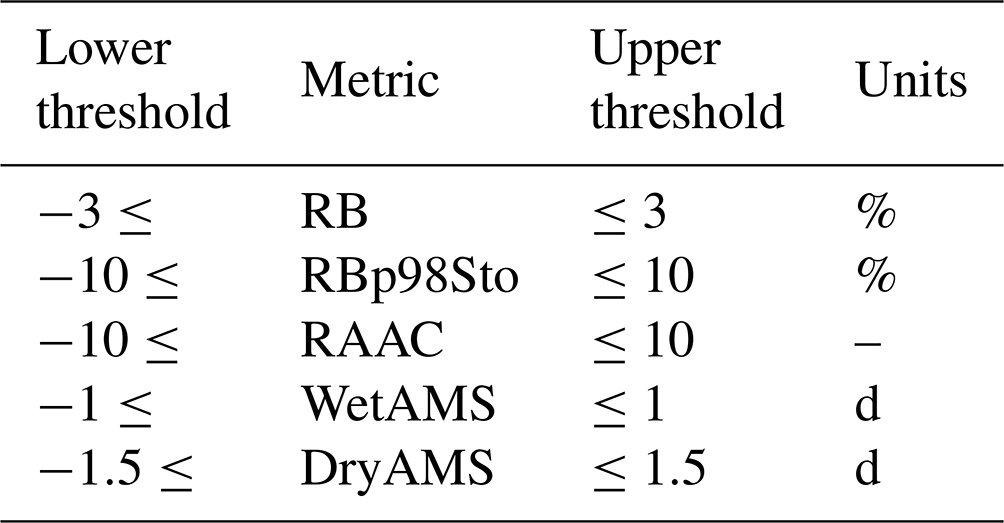
The metrics shown in Table 1 were computed for the independent validation dataset (2010–2015). The performance of each metric per individual model was ranked, and then the sum of all the individual ranks was employed to obtain an overall rank. Also, it was observed that for 297 transfer functions, at least one pixel was returning not real numbers, therefore these models were excluded from the analysis, although the reasons behind their “failure” are discussed later on. After reviewing the resulting ranking, it was noticed that some of the metrics of the best performing models were not satisfactory, e.g. high ROCSS and Spearman correlation but poor performance of the spells, WetAMS, and DryAMS, the latter being the most challenging metric to accurately model. Therefore, to short-list and decide which models to select, the conditions shown in Table 2 were applied to the median validation metrics, which reduced the number of transfer functions that complied to 35.

Table 2 Conditions applied to the median validation metric values of the transfer functions for further pruning.

After implementing the aforementioned conditions, the best CNN1 (none of the 10 runs complied) and the best 11 performing architectures were selected and further analysed, i.e. duplicated architectures like U-3-64-1-T (overall ranked #2 and #11) and Upp-3-64-1-F (#3 and #20) were removed to show the performance of different ones. Boxplots of the validation performance metrics of selected models are shown in Fig. 3.

In general, the performance of the U-like models exceeds the one of the benchmark, CNN1, for most of the metrics with respect to both the median and the variability of the results. Note that the best run of CNN1 is ranked #484 out of the remaining 703 models. DryAMS is the major weakness for CNN1, yet ROCSS, Spearman correlation, and RMSE are also unsatisfactory, which are key to the overall performance. Also, the variability of the RB-based metrics and RMSE is quite large compared to most of the other models, as shown by the span of the whiskers.

Particularly, the #1 ranked model, Upp-4-128-3-F, was initially excluded from the analysis because of its high DryAMS bias (see the unpruned analogous to Fig. 3 in Fig. A1). Further examination revealed that the variability of its metrics is considerably higher than for other models and only 3 out of the 10 runs of this architecture did not end as “failures”, so that this particular exceptional performance could have been a matter of happenstance rather than the architecture being optimal for the task.

It is worth noting that CNN1 comprises 5 912 251 parameters while ranked #2 architecture U-3-64-1-T, and ranked #3 architecture Upp-3-64-1-F include 7 769 465 and 7 950 389 parameters, respectively. This reaffirms the performance improvement induced by the skip connections with a rather minor proportional increase in the number of parameters. However, the robustness provided by both architectures takes around three- and fourfold training time per step (20 steps per epoch for all the models), respectively, which sums up to between five- and sevenfold the total training time for #2 and #3 (see Table 3).

Table 3 Computational details of some of the models. Note that some models not shown before, like Upp-5-128-3-T, which was the largest model trained, are added for completeness. All the following calculations were carried out on a NVIDIA A-100 (40 GB) GPU, with a batch size of 512, resulting in 20 steps per epoch. The table is ordered according to the ascending number of total parameters in the models.

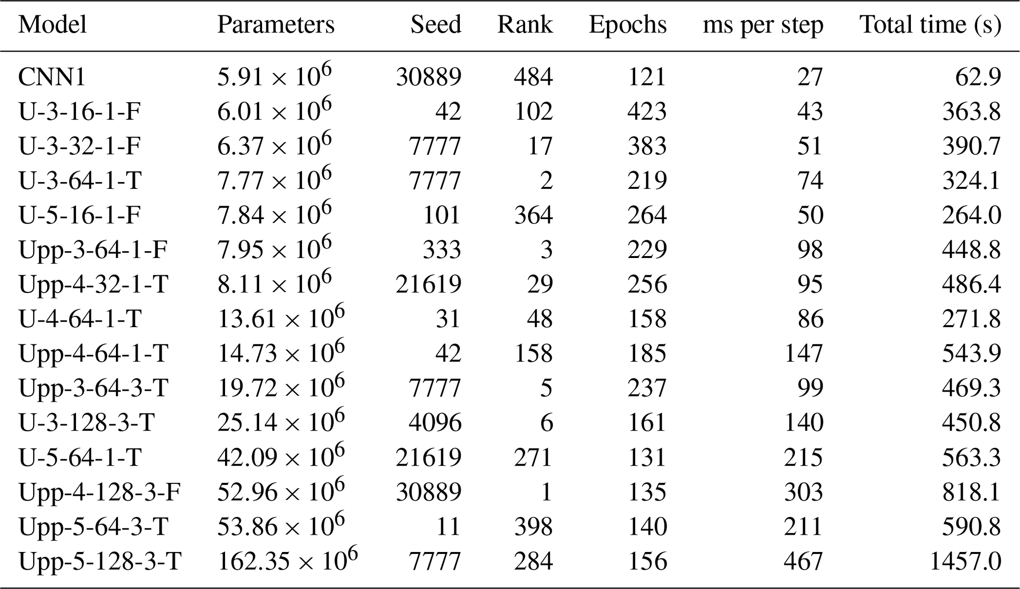
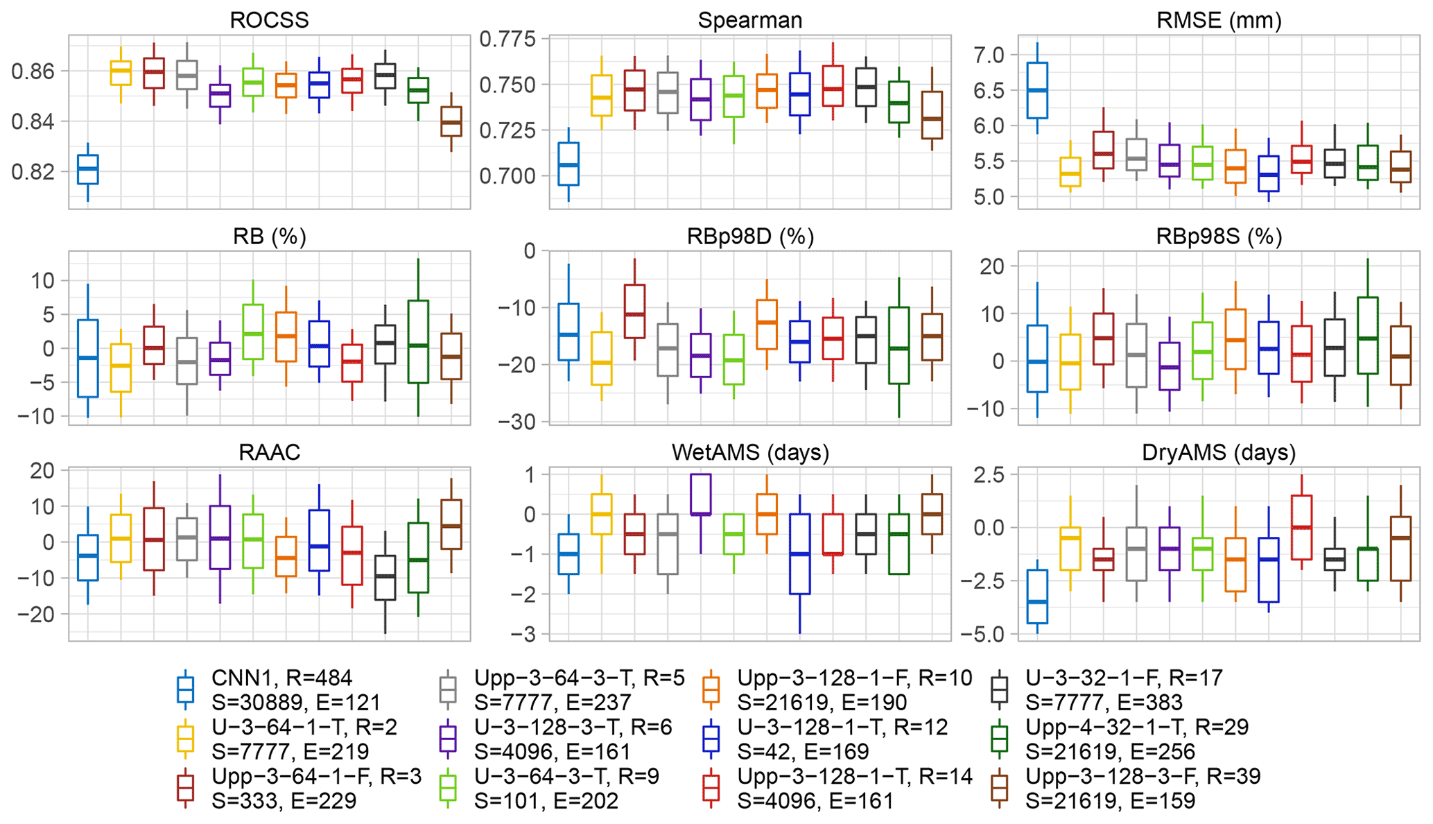
Figure 3 Validation metrics of CNN1 (benchmark) and the 11 best-performing architectures after pruning, ordered according to their rankings. Each sub-panel contains 12 boxplots, one per model, which summarizes the results for the 1916 pixels within the Eastern Ore Mountains. The boxes comprise the 25th and 75th percentile and the median, the whiskers the 10th and 90th percentile. The letters D and S after RBp98 stand for deterministic and stochastic approaches, respectively. Note that in the legend, ordered column-wise, alongside the nomenclature of the models details are added such as the overall ranking (R), the random seed number (S) of the run, and the number of epochs (E) needed to train the transfer functions (due to the patience of 75, the shown performance was achieved in E-75 epochs).

Additionally, in the training–validation loss plots for CNN1 (see Fig. A2), it was observed that shortly after reaching the minimum, the validation loss curve started to diverge from the training loss one, which can be interpreted as overfitting of the model and explains the relative small number of epochs needed during training, due to the patience set. This behaviour was not observed for the U-like architectures or is at least not so evident as for CNN1. Still, since only the best model per architecture was saved during training before early stopping, the performance metrics were not compromised, yet the model architecture might not be ideal for the task at hand.

The model ranked #2 (U-3-64-1-T) is considerably superior to the other ones with respect to most of the validation metrics. This includes the lower variance for most of the variables, and a clear advantage on RMSE and the spells (−0.5 median value for both), which were rather hard tasks for most of the models and are key performance metrics for potential subsequent impact modelling use of the downscaling output.

Noticeably, the RBp98, under a deterministic approach, is the metric with the poorest behaviour overall, which is between −10 % and −20 % for most of the transfer functions. This could be explained by the joint effect of the already shown RB in Fig. 1a and the extreme events of 2013, included in the independent validation metrics calculation only. Nevertheless, the stochastic approach shows a satisfactory performance, although it should be used carefully, since the temporal and spatial structure is lost due to its underlying logic (Baño-Medina et al., 2020), as observed in the RBp98S row of Fig. 4. Therefore, longer-term averages and/or aggregated regions would be an appropriate use case for the datasets generated under this procedure.

Figure 4 Spatially distributed validation metrics, row-wise, of CNN1 (benchmark) and a sub-selection of the best performing models. The numbers inside the panels represent the overall median of the metrics amongst the Eastern Ore Mountains domain. Note the shared scales among the metrics.

The first six models shown in Fig. 3 were chosen to further assess the spatial distribution of the metrics, as shown in Fig. 4. Both ROCSS and Spearman correlation have a rather smooth spatial distribution of their values, with a noticeable decrease in its performance in the south-eastern corner of the region for all the models, as seen in Fig. 4. The median RB of CNN1 is −1.42 %, but its high variability can be noticed, particularly towards the north-west of the Eastern Ore Mountains, while e.g. #2 (median −2.57 %) shows a smoother distribution. The median RB of U-3-64-3-T is better than for #2 but has a noisier behaviour, which depending on the application of the downscaled datasets, could play an important role.

In case of RBp98 under deterministic conditions, Upp-3-64-1-F has the best overall results with intermediate variability. Generally, smoother contrasts are seen for the U-like models for most of the metrics. RAAC shows high spatially distributed discrepancies, particularly for U-3-128-3-T and U-3-64-3-T, with very low values in the north-west and intense positive deviations in the south-east. Smaller but consistent differences are seen for most of the models.

During the analysis it was evident that the “full size” of the U-like architectures, five layers, did not provide the best performance, which in computer vision assignments tends to excel. This finding could be partially explained by the relative small size of the domain, 32 by 32 pixels. Because of the domain side halving logic enforced by these architectures on each layer, joined with the lack of extra padding, the remaining domain size in the fifth layer was only 2 by 2, which possibly limits the efficiency of the models. Also, overfitting might have played a significant role ruling out the larger models. Generally, the smaller models achieved better performances, which could change with a larger predictor domain size, e.g. 64 by 64.

Furthermore, it seems that the starting point in the loss function topology plays a significant role in the transfer function performance, particularly under the early stopping settings used. Therefore, further assessments of the balance between the number of different seeds numbers, early stopping, and total calculation time should be carried out for similar future applications, in order to optimize GPU time use. With the same purpose in mind, batch size could be programmed to be a transfer function dependent number for GPU memory use optimization.

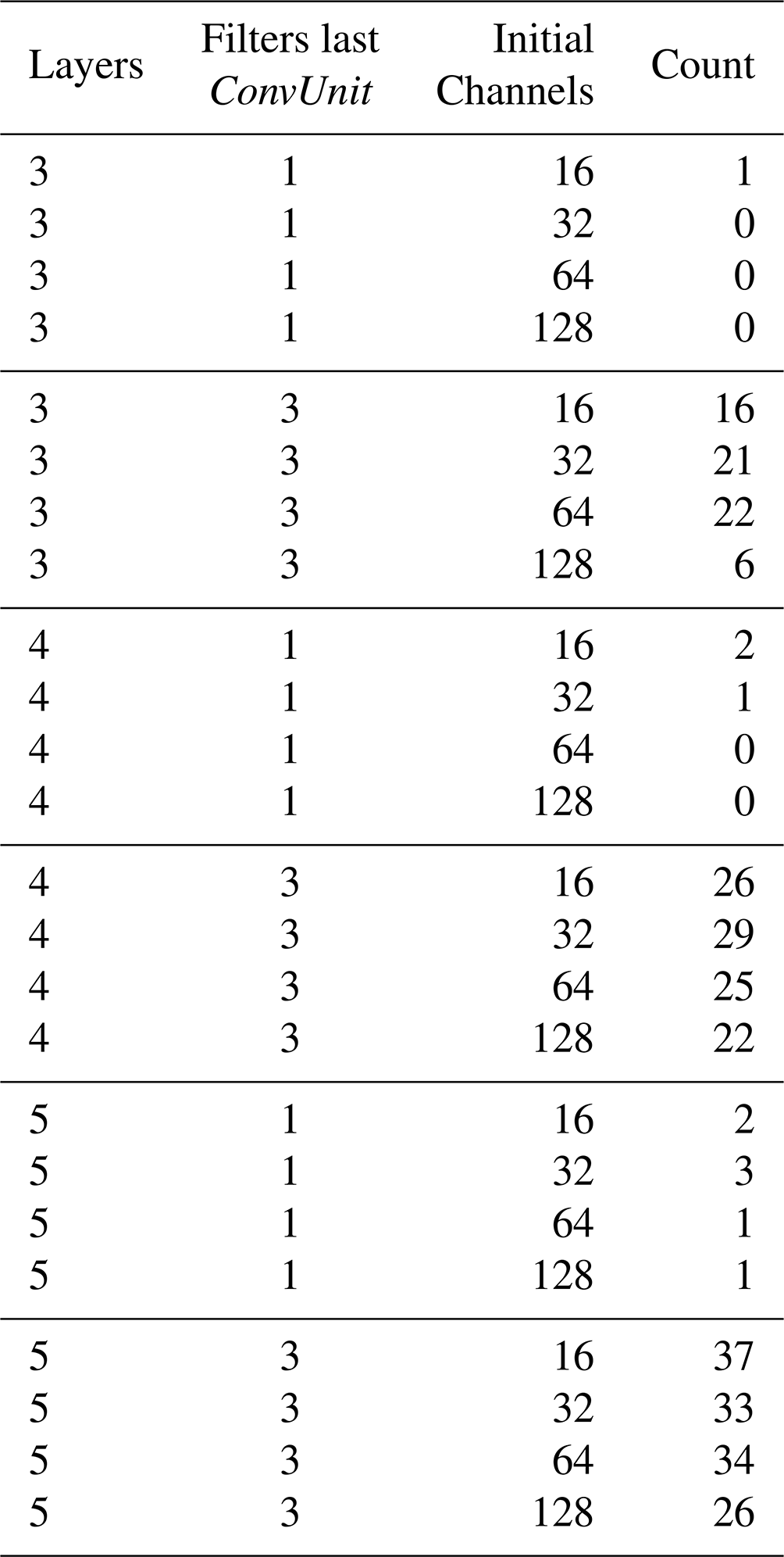
Regarding the transfer functions that resulted in non-real numbers in at least one pixel of the whole domain (297 cases), a couple of noteworthy details were found. First, the type of U architecture and number of initial channels did not seem to be a decisive factor: 153 were U-Net and 144 U-Net++. This small difference could be explained due to the added robustness of the additional skip connections given by the latter architecture. Furthermore, 84, 87, 71, and 55 “failed” transfer functions were related to models with 16, 32, 64, and 128 initial feature channels, respectively. The random seed number or “starting point” appears to have considerable influence on the “failed” models: seed=11 is related to 36 failures, while the most successful one had 22 (seed=7777). Table 4 is shown to better understand the influence of some hyperparameters on the failure of the models.

Table 4 Grouping of the transfer functions resulting in non-real number values in at least one pixel in the Eastern Ore Mountains domain, according to number of filters in the last ConvUnit and batch normalization condition.

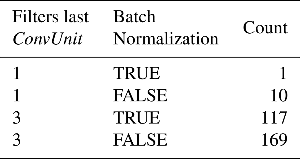
Note that only one model corresponds to the combination of one feature channel on the last ConvUnit with batch normalization and 10 without it, which could mean that the extra parameters (three channels) on the last layer add noise to the model that results more frequently in non-real values. Furthermore, not applying batch normalization to the last ConvUnit leads to a greater number of failures (179 versus 118). Therefore, it is suggested for subsequent studies to use batch normalization with a single channel on the last layer. Models with larger numbers of layers and initial channels (see Table A1 and Table A2), and therefore larger total numbers of parameters, tend to “fail” with the independent validation dataset more often than the smaller ones, probably due to overfitting. Combinations of three filters in the last ConvUnit with no batch normalization “failed” more often than their normalized counterparts, and this behaviour augmented with the number of layers of the U-like architectures. Furthermore, a lower number of initial channels (16 and 32) tends to “fail” more often and this behaviour increases with the depth of the U-like structure. This “failure” probably happens when the transfer function can not handle unseen conditions during training (lack of extrapolation capability) and is related to hyperparameters that form a more “rugged“ loss function topology, permitting under- and overfitting of the models.

4.2 Repeatability

As mentioned previously, general reproducibility is a notorious issue for both climate science and GPU-based calculations. In addition, deep learning techniques are not yet completely approved by the climate community, mostly due to interpretability concerns, deepened by the general reproducibility ones. Therefore, attempting to provide a repeatable framework was a cornerstone enterprise of the study while being aware of the properties and limitations of both the hardware and software. Thus, Fig. 5 presents the experiment described in 3.5, showing five of the validation metrics and the minimum Bernoulli Gamma loss function value from the 10 different runs for the benchmark CNN1, and the models ranked #2 to #3 under both deterministic and non-deterministic conditions.

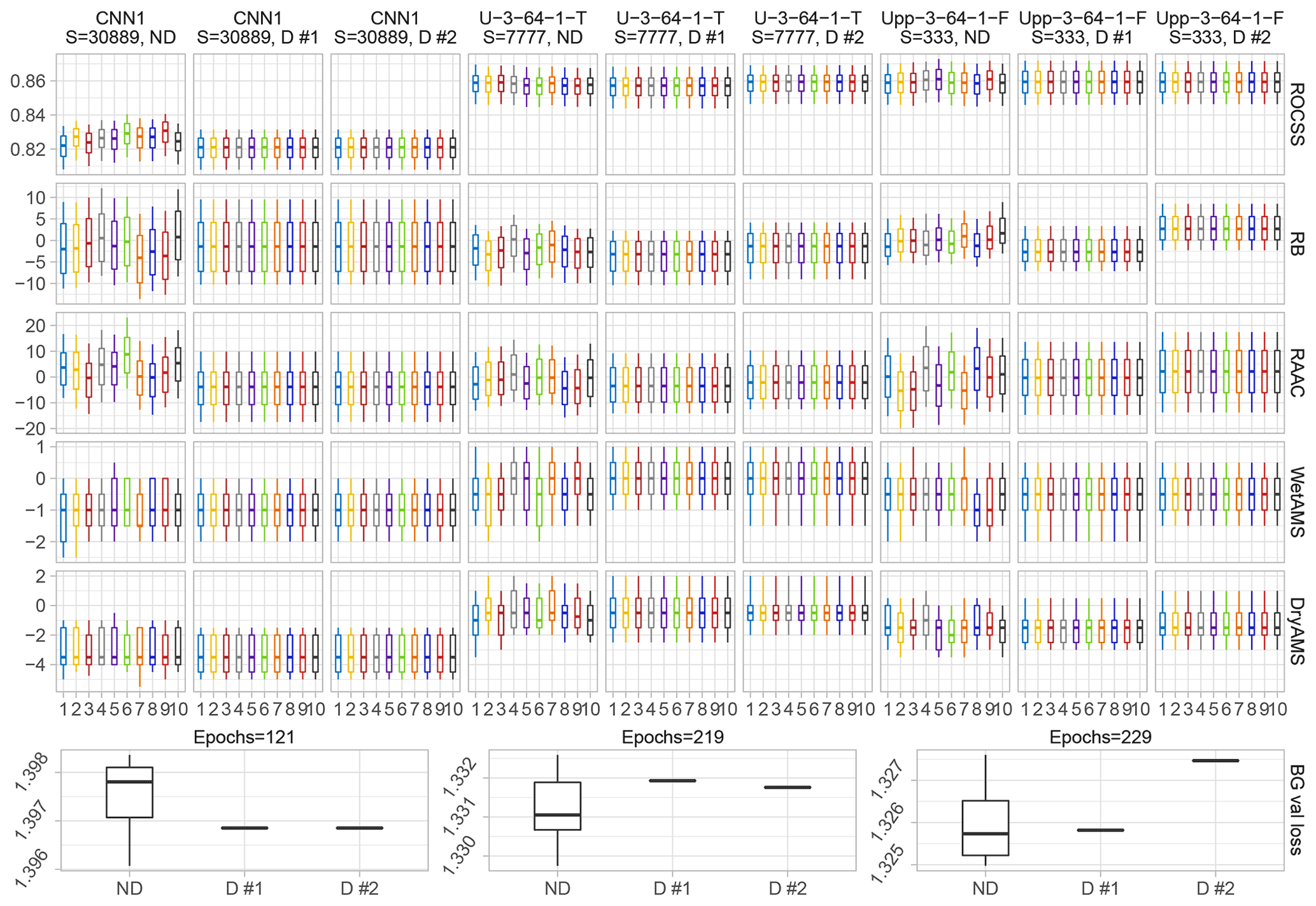
Figure 5 Comparison among 10 runs under the same seed number and configuration for the benchmark, and a sub-selection of the best performing transfer functions ordered column-wise. A sub-selection of the metrics from Table 1 is shown row-wise plus a row which depicts the boxplots of the minimum value achieved by the Bernoulli Gamma loss function (BG val loss) during training per type of run and model. D stands for deterministic and ND for non-deterministic runs. Note that all the runs per model needed the same amount of epochs.

As noticeable from Fig. 5, all the 10 deterministic runs of the same model result, as expected, in the exact same outcome. Thus, repeatability was achieved. Yet, depending on which specific GPU out of the 272 same ones available in Alpha Centauri is used, minor differences can be observed among them, despite complying with the conditions that reportedly guarantee determinism (see Sect. 3.5). Both deterministic repetitions for CNN1 were done on the same physical GPU, therefore all of the 20 runs resulted in the exact same value for all metrics and pixels. In the case of the repetitions for U-3-64-1-T and Upp-3-64-1-F, which were trained on different physical GPUs of the same sub-cluster (same hardware) using the same source code and container, minor variations among them were observed, which can be interpreted as the aforementioned similarity. Despite not being able to exactly repeat the outcomes under different GPUs, the hereby presented results are quite satisfactory for the scope of this project.

From the non-deterministic runs shown in Fig. 5 it can also be observed that the variability of the results was considerably narrowed down, through the containerization of the environment and the seeding of the random numbers, which can also be interpreted as a measure of similarity. The latter can be seen in the last row of the aforementioned figure, where e.g. the minimum in-training Bernoulli Gamma validation loss function for the different configurations start to differ in the third or fourth decimal place. Nevertheless, strong variations are observed within the different runs per model, which might lead to some runs having a substantial better performance than the remaining ones without a foreseeable reason rather than randomness and non-determinism. Lastly, it is worth noting that the non-deterministic runs were calculated faster, e.g. 23 ms per step instead of 27 for CNN1, 71 instead of 74 for U-3-64-1-T, and 90 instead of 98 for Upp-3-64-1-F.

4.3 Suitability of the architectures

The deterministic results presented in Sect. 4.2 constitute the last iteration of the present project. However, before achieving this cornerstone, non-deterministic operations were employed and several noteworthy details regarding the suitability of the architectures for this particular task were found, which we believe deserve a place in the present discussion. Figure 6 shows a sub-selection of transfer functions chosen to illustrate some of these features.

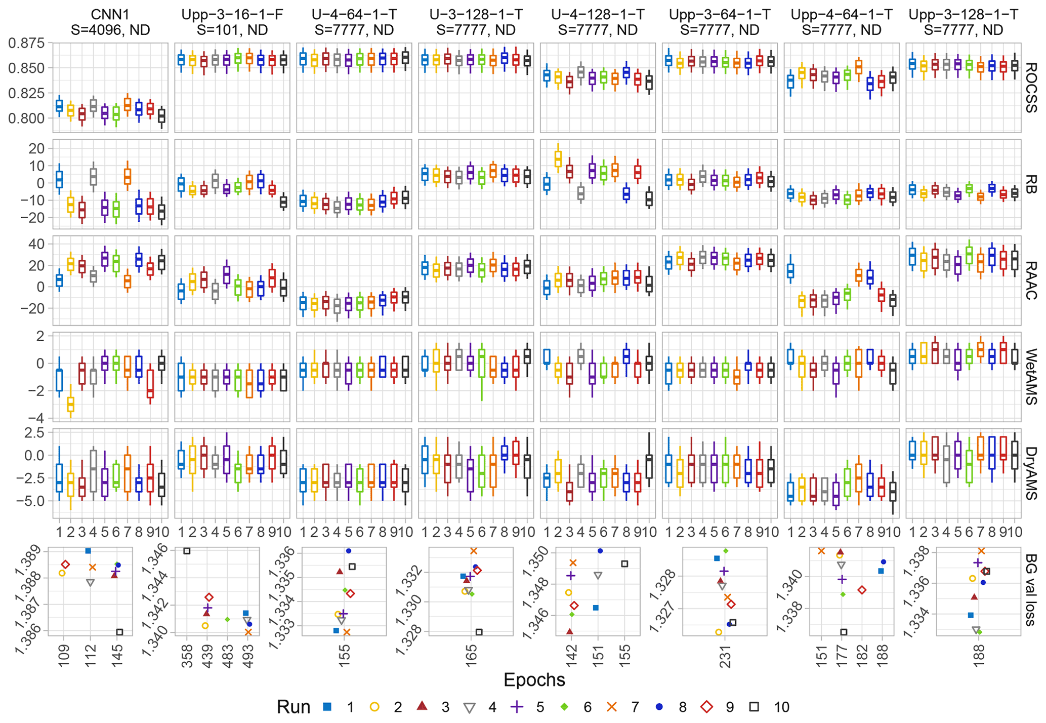
Figure 6 Similar to Fig. 5 but for other architectures under non-deterministic conditions only. The last row depicts the minimum value achieved by the Bernoulli Gamma loss function (BG val loss) during training and the number of epochs needed to train the models. Note that the x axis of the last row is not to scale and the symbols are avoiding other ones on similar positions to ease its readability, thus refer to the closest abscissa grid line to interpret its epoch.

Initially, it can be observed that some runs of the same architecture needed different number of epochs to train, categorized in one to four scenarios, in contrast to the results shown in Fig. 5. We believe that the number of training scenarios can be interpreted as a measure of model suitability or of how rugged its loss function topology is, which is in turn related to under- or overfitting of the models (see Fig. A2). A lower number of scenarios under non-deterministic conditions implies that the inherent noise is to a certain extent suppressed. In the case of CNN1 for seed=4096, three scenarios were identified with 112 epochs being clearly the best performing one. Three out of the 10 runs fell into this scenario (1, 4, and 7), which confirms that depending on the architecture, the best result might be a matter of randomness. The same behaviour can be observed for other architectures with multiple training scenarios and can be interpreted as a measure of dissimilarity.

Notably, the hyperparameters mentioned in Sect. 4.1, which did not result in non-real values (i.e. batch normalization, three or four layers, just one channel in the last ConvUnit, and 64 or 128 initial feature channels) are the ones that generally lead towards a more stable or smooth loss function, which in turn may reduce the number of training scenarios under non-deterministic conditions, producing similar outcomes. On the other hand, the 16 initial filters and no batch normalization of Upp-3-16-1-F might result in a rather rugged loss function topology. The aforementioned architecture produced four different training epochs scenarios, which decrease its suitability and similarity. Thus, for the specific conditions of the present task, the combination of three layers with either 64 and 128 filters, or four layers with 64 filters, one channel, and batch normalization in the last ConvUnit for both U-like models, is the sweet-spot for the architecture suitability.

5 Summary and outlook

Deep learning methods have substantially developed over recent years in various domains, with computer vision studies focused on medical imaging often being pioneers. However, there are still interpretability concerns with deep learning models and well-known general reproducibility issues with GPU accelerated calculations (Jézéquel et al., 2015; Nagarajan et al., 2018; Alahmari et al., 2020). Nevertheless, there are various recent studies including algorithms such as CNNs for statistical downscaling applications with promising outcomes, Baño-Medina et al. (2020) being the benchmark for the present study. However, the aforementioned study did not include recent architectures such as U-Net and U-Net++ nor GPU accelerated calculations.

Considering the costs of developing worldwide physically based projections on an impact-model-relevant scale, and the urgency with which this information is required, we therefore focused our efforts on improving the building blocks to use deep learning towards repeatable high-resolution statistical downscaling, particularly with a methodology extendable to other regions, spatio-temporal scales, and diverse variables while taking advantage of state-of-the-art architectures and hardware.

A hyperparameter-space search including 100 distinct models was carried out applying 10 different seed numbers to examine their optimum values and patterns in both performance and repeatability terms. In general, the skip connections-based models performed significantly better than the best run of the benchmark CNN1 in both median and variability terms for the performance metrics taken from the VALUE framework. U-3-64-1-T was the overall best-performing model for the present arrangement, considering the configuration of input channels and numbers of input and output pixels, which consist of three layers with 64, 128, and 256 feature channels, respectively, and a single channel with batch normalization on the convolutional layer after the U-Net structure. The latter is in terms of deep learning a rather simple model. Its total number of parameters is 7.77 million, which in contrast to the 5.91 million parameters of CNN1, represents a strong improvement without major computing requirements. The total training time for the aforementioned model was approximately 6 min with one NVIDIA A-100 GPU, under the shown configuration.

The hereby presented workflow demonstrated satisfactory performance to downscale daily precipitation using as predictors 20 variables of the ERA5 reanalysis to a resolution of 1 km, offered by the ReKIS dataset. Though the method is in principle able to work with station data too, benefiting from spatially distributed predictors, its clear advantages are the result fields, e.g. needed for impact modelling with lateral exchange like hydrological modelling. Besides the here applied geostatistical product ReKIS, e.g. in regions or for variables with less dense measurement networks, regional reanalysis products like COSMO-REA2 (Wahl et al., 2017) can be employed. The outcomes of the method were validated through the robust VALUE framework, while building upon the climate4R structure, which due to the reach of R in several related fields, could prove greatly beneficial for further associated and/or derived studies.

Furthermore, the presented transfer functions, and other ones to be derived for additional variables, will be applied to the EURO-CORDEX 0.11^∘ ensemble. The latter offers a greater amount of GCM–RCM variables than EURO-CORDEX 0.22^∘. Thus, a rather straightforward upsampling method could be enough to match the EURO-CORDEX 0.11^∘ and ERA5 grids. The projections for the Eastern Ore Mountains are then intended to serve as input to multi-purpose impact models, such as hydrological, agronomic and ecological ones.

The Singularity container developed for the present task allowed further scrutiny of the GPU deterministic implementations, repeatability capabilities, and the suitability of the different architectures tested. Full repeatability was achieved when using the exact same physical GPU. A high degree of similarity was accomplished among runs on different GPUs, even though we complied with the reported conditions for repeatability, hardware- and software-wise. Still, this is a highly satisfying outcome. The models were trained on state-of-the-art hardware (Alpha Centauri sub-cluster), nevertheless they can be recalculated, with the corresponding adjustments in, e.g. batch size and subsequent learning rate changes, on alternative GPU models or on CPU.

The presented approach addresses the underlying general reproducibility issues while complying with the conditions for methods reproducibility (Goodman et al., 2016). The achieved repeatability is essential to build trust in deep learning applications and to further develop towards interpretable models. The latter is particularly relevant for statistical downscaling, where interpretability of the transfer functions is fundamental to trustfully downscale projected climate change scenarios.

Appendix A

Figure A1 Same as Fig. 3 but without the filtering conditions applied.

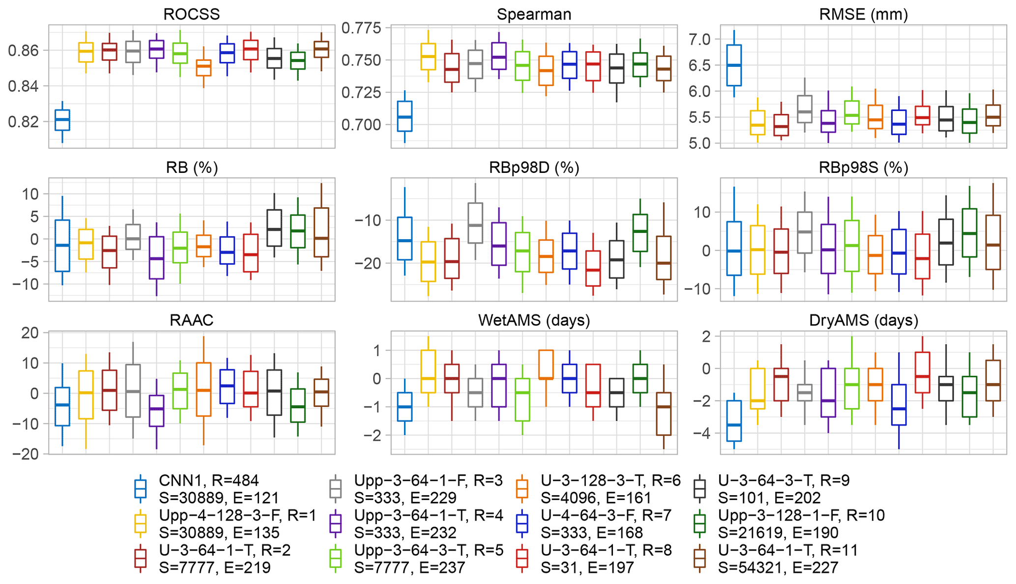
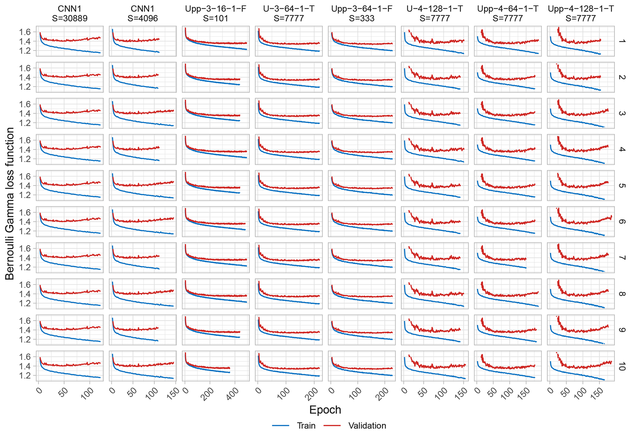
Figure A2 Training-validation loss plots for 10 runs under the same random seed number and configuration for the benchmark and a sub-selection of the transfer functions under non-deterministic conditions, ordered column-wise.

Table A1 Similar to Table 4 but grouped according to amount of layers, filters in the last ConvUnit, and batch normalization.

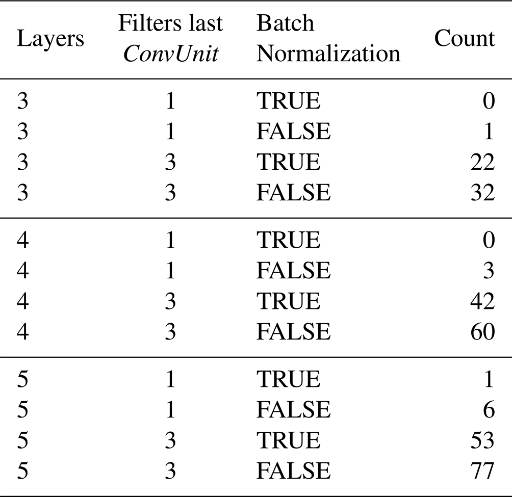
Table A2 Similar to Table 4 but grouped according to amount of layers, filters in the last ConvUnit, and initial feature channels.