the Creative Commons Attribution 4.0 License.
the Creative Commons Attribution 4.0 License.
 | 04 Oct 2022
Water balance model (WBM) v.1.0.0: a scalable gridded global hydrologic model with water-tracking functionality
Danielle S. Grogan
Alex Prusevich
Wilfred M. Wollheim
Stanley Glidden
Richard B. Lammers
This paper describes the University of New Hampshire Water Balance Model, WBM, a process-based gridded global hydrologic model that simulates the land surface components of the global water cycle and includes water extraction for use in agriculture and domestic sectors. The WBM was first published in 1989; here, we describe the first fully open-source WBM version (v.1.0.0). Earlier descriptions of WBM methods provide the foundation for the most recent model version that is detailed here. We present an overview of the model functionality, utility, and evaluation of simulated global river discharge and irrigation water use. This new version adds a novel suite of water source tracking modules that enable the analysis of flow-path histories on water supply. A key feature of WBM v.1.0.0 is the ability to identify the partitioning of sources for each stock or flux within the model. Three different categories of tracking are available: (1) primary inputs of water to the surface of the terrestrial hydrologic cycle (liquid precipitation, snowmelt, glacier melt, and unsustainable groundwater); (2) water that has been extracted for human use and returned to the terrestrial hydrologic system; and (3) runoff originating from user-defined spatial land units. Such component tracking provides a more fully transparent model in that users can identify the underlying mechanisms generating the simulated behavior. We find that WBM v.1.0.0 simulates global river discharge and irrigation water withdrawals well, even with default parameter settings, and for the first time, we are able to show how the simulation arrives at these fluxes by using the novel tracking functions.
- Article
(8849 KB) - Full-text XML
-
Supplement
(2210 KB) - BibTeX
- EndNote


Global hydrologic models (GHMs) are one of the primary tools used in the study of macro-scale hydrology, and the past 30 years have seen the development of numerous GHMs. These include the following models water balance model (WBM; Vörösmarty et al., 1989), VIC (Liang et al., 1994), WaterGAP (Döll et al., 2003), H08 (Hanasaki et al., 2008a, b), PCR-GLOBWB (Sutanudjaja et al., 2018), and others (Telteu et al., 2021). The terrestrial hydrology concepts and structures from these models have now been incorporated into several land surface models (LSMs), e.g., NASA LIS (Kumar et al., 2006) and the Community Land Model (CLM; Lawrence et al., 2019), and Earth system models (ESMs) such as and WRF-Hydro (Gochis et al., 2020) and the Community Earth System Model (CESM; Zeng et al., 2015), and others such as the U.S. National Water Model (NWM; Cohen et al., 2018). The GHMs represent the land surface component of the hydrologic cycle, converting time series of weather and land-cover variables into estimates of water storage and flux values. These models have been applied to many questions of both basic and applied hydrology, such as climate change and other anthropogenic impacts on global river systems (Bosmans et al., 2017; Döll et al., 2012; Haddeland et al., 2014; Hanasaki et al., 2008b; Vörösmarty et al., 2000a, 2010; Wada et al., 2011), groundwater depletion (Döll et al., 2014; Gleeson et al., 2012; Grogan et al., 2017; Wada et al., 2012), and the role of water extractions in sea-level change (Gleeson et al., 2012; Konikow, 2011; Pokhrel et al., 2012). The GHMs have also been used extensively in the study of food security and agricultural yields (Biemans and Siderius, 2019; Döll and Siebert, 2002; Elliott et al., 2014; Haqiqi et al., 2021; Liu et al., 2017; Schewe et al., 2014) as well as formed the foundation for water quality models (Mineau et al., 2015; Stewart et al., 2011; de Wit, 2001; Wollheim et al., 2008a, b; Zuidema et al., 2018) and the inputs for flood inundation models (e.g., Yamazaki et al., 2011). Recently, GHMs have been employed in interdisciplinary studies to evaluate human–hydrologic systems and the food–energy–water nexus, such as human and economic impacts of flooding (Dottori et al., 2018), hydropower (Mishra et al., 2020; Turner et al., 2019), power-plant cooling capacity (van Beek et al., 2012; Stewart et al., 2013; Webster et al., 2022), water markets (Rimsaite et al., 2021), irrigation decision-making under climate change (Zaveri et al., 2016), and virtual water trade (Dalin et al., 2017; Konar et al., 2013). Recent overviews of GHM literature are also provided in Sutanudjaja et al. (2018) and Telteu et al. (2021).
The GHMs were developed to quantify land surface hydrologic fluxes at global and continental scales, and these models generally capture the macro-scale behavior of the water cycle in both natural and human systems (Telteu et al., 2021). Model limitations include poor simulation during low runoff periods and a tendency to overestimate mean annual runoff and discharge (Zaherpour et al., 2018). While early GHMs only represented natural hydrologic fluxes, the recent addition of human impacts were shown to greatly improve river discharge estimates and in most cases, lowered the overly high estimates of average annual river flow (Veldkamp et al., 2018). Despite these improvements, there have been calls to better represent regional water management, co-evolution of the human–water system and improved human water management information in GHMs (Wada et al., 2017). A large challenge for macro-scale hydrological modelers is to better capture the human decision-making around water movement, use, and consumption. One method for achieving this is by linking models from the social sciences to hydrological models (e.g., Mishra et al., 2020; Webster et al., 2022; Zaveri et al., 2016). The model described in this paper, WBM v.1.0.0, captures all the major land surface water stocks and fluxes with a focus on human alterations of the water cycle. A significant contribution of this model version is the ability to track water, depending on its source or use through the entirety of the system, highlighting how movement of water for human use interacts with the natural water system.
Tracking water sources
As pressures on water resources increase through both climate change and intensifying human water demand (e.g., Vörösmarty et al., 2000a), it is important to know the origin of regional water resources. While some basins may be supplied by steady precipitation or recharging aquifers, others rely on seasonal snowpack, fossil groundwater, irrigation returns, glacial melt, or monsoon rains. Each of these water sources comes with their own set of management challenges and opportunities, making knowledge of water sources a vital component of water resource planning. It may seem obvious where a basin or region's water comes from; however, human water use introduces complexities into the terrestrial water cycle that can obscure the often lengthy and circuitous pathway that waters take from source to use (Grogan et al., 2017; Zuidema et al., 2020). The discussion here is confined to the terrestrial water cycle since GHMs do not, by definition, simulate the atmosphere. Under natural conditions, most of the water that enters a river basin travels from the land surface through soils, groundwater through headwater basins (Alexander et al., 2007), and then through the full river system to the ocean or endorheic outlet. Humans withdraw large quantities of water from these natural pathways and because no activity of human water use is completely consumptive, water extracted from river and groundwater systems is returned either to its original source or diverted to an alternate pool. Irrigation accounts for ∼70 % of all freshwater withdrawals (Rosegrant and Cai, 2002), and is ∼50 % is efficient globally (Döll and Siebert, 2002; Gleick et al., 1993), returning approximately half of all extracted irrigation water back to surface water and groundwater storages. The repetition of this activity causes iterative cycles of water extraction and return over annual to decadal time scales, creating complex, circuitous pathways. The pathways that water travels impact water quality (Huang et al., 2022; Mineau et al., 2015), food security (Kadiresan and Khanal, 2018), and governance of water resources through transboundary interactions (Zeitoun and Mirumachi, 2008). Furthermore, humans develop hydro-infrastructure to intentionally impound (Lehner et al., 2011; Zuidema and Morrison, 2020) and divert rivers (Ghassemi and White, 2007), and engage in artificial recharge of groundwater pools (Dillon et al., 2019). These activities divert water through natural and artificial stocks, masking the identity of the original source of the water.
Understanding the journey of certain sources of water illuminates their role in downstream water resource issues and how human-induced complex pathways make the attribution of upstream changes to downstream effects increasingly difficult. In this paper, we present three examples of tracking water parcels through the hydrological cycle by preserving key attributes related to water sources, return flows from water extraction, and an identifier assigned to all runoff generated from a given land area. This novel modeling method maintains the identity of a water parcel as it travels through natural and anthropogenic pathways, illuminating previously obscured connections between sources, uses and fates, as well as offering a potential useful tool for understanding water quality changes throughout watersheds.
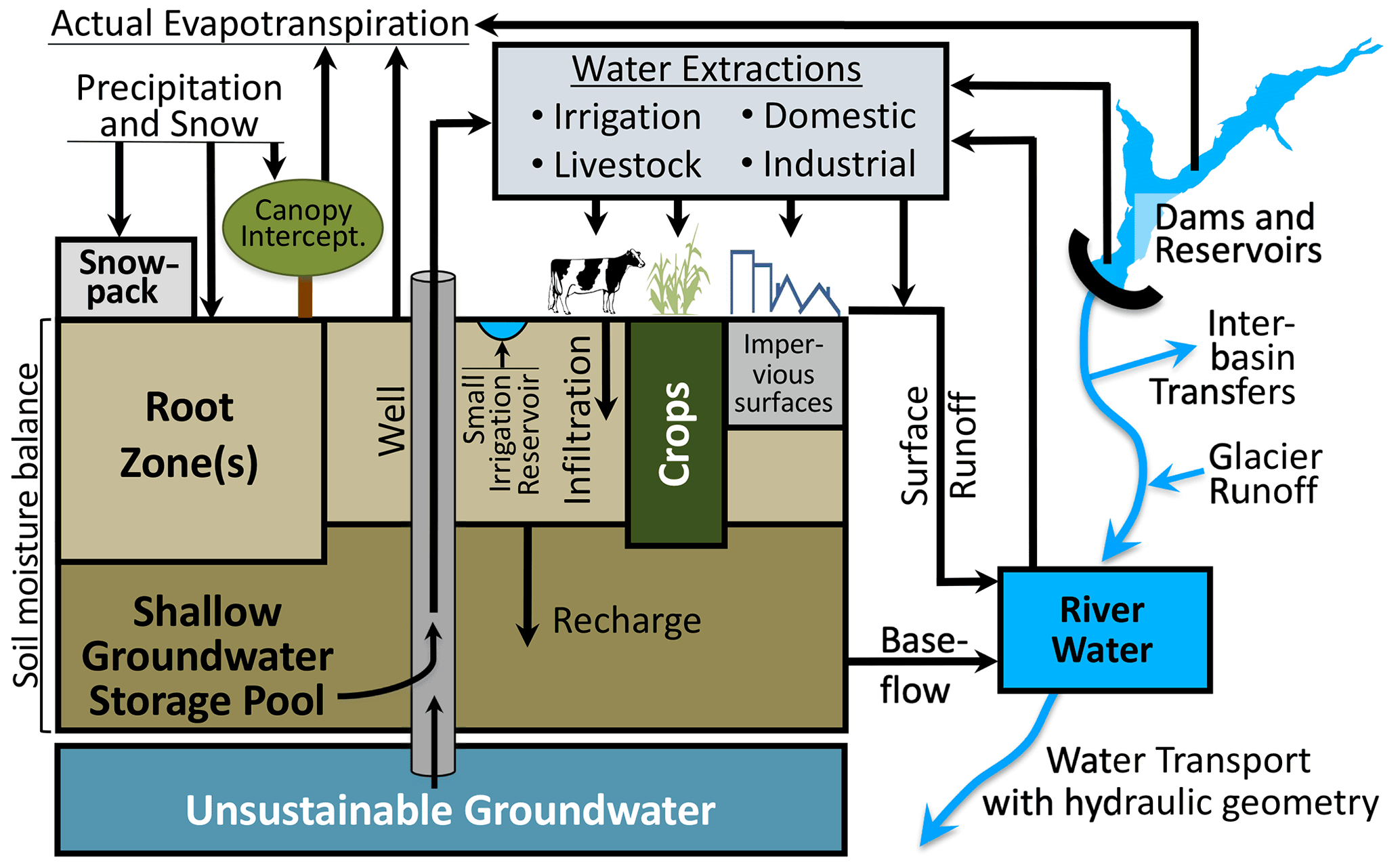
Figure 1Schematic representation of the water balance model (WBM) showing major fluxes and storages, which are described in Sect. 2.2.1–2.2.6 below. The land surface fluxes are described in Sect. 2.2.1, and are: precipitation and snow, canopy interception, open water, runoff from impervious surfaces, soil moisture balance, actual evapotranspiration, surface runoff, and glacier runoff. Both the shallow groundwater storage pool and the unsustainable groundwater are described in Sect. 2.2.2. River water, including baseflow and hydraulic geometry, is described in Sect. 2.2.3. Section 2.2.4 describes dams and reservoirs, inter-basin transfers, and small irrigation reservoirs. All water extractions are described in Sect. 2.2.5. The model operates on daily time steps and over grid cells defined by the digital river network. Grid-cell resolutions have been used in the range from 30 arcmin to 120 m.
In this paper, we provide a detailed description of WBM v.1.0.0, its performance compared to observations of global hydrologic fluxes when using default parameterizations, and examples of how the tracking functionality can be used to evaluate the role of human alterations to the global hydrologic cycle. We review previous studies that have used earlier versions of WBM, and provide guidance for setting up and running WBM v.1.0.0.
2.1 General overview
The WBM (Grogan, 2016; Wisser et al., 2010a) is a process-based, gridded hydrologic model that simulates spatially and temporally varying water volumes and quality (Fig. 1), operating at daily time steps. It was one of the first GHMs developed (Vörösmarty et al., 1989), and is now joined by many other similar GHMs and LSMs in its representation of the terrestrial portion of the water cycle. The WBM represents all major land surface components of the hydrologic cycle, and tracks fluxes and balances between the atmosphere, above-ground water storages (e.g., snowpack), soil, vegetation, groundwater, and runoff. A digitized river network connects each grid cell to the next, enabling simulation of flow through river systems. The WBM includes domestic and industrial water requirements and use, agricultural water requirements and use (irrigation and livestock), and hydro-infrastructure (dams and inter-basin transfers). While the model is considered global, it can be run for any region and any spatial resolution, given available input data at the appropriate scale. For example, WBM has been operated at a local scale of ∼120 m grid-cell resolution over a 400 km2 watershed (Stewart et al., 2011), and at global scales (Grogan et al., 2017; Wisser et al., 2010a) (Table A1).
The WBM is modular and is able to accept climate, land use/land cover, water management, and water demand inputs from other models and data sources, such as glacier melt models (e.g., Huss and Hock, 2015; Rounce et al., 2020a, b), reservoir operation data (Zuidema et al., 2020), or econometric land use models (Zaveri et al., 2016). The modular components can be turned on or off with binary flags in a model initialization file. The modular components can be turned on or off with binary flags in a model initialization file. Users can select any combination of the following anthropogenic processes: (1) water extraction for irrigation, (2) rainfed crop water evapotranspiration (ET), (3) water use for livestock, municipalities, and industrial production, (4) inter-basin transfers, and (5) reservoirs and dams. In contexts where water quality is simulated, fluxes of solutes from other models such as the terrestrial biogeochemical model PnET (Aber et al., 1997) provide the relevant boundary conditions to WBM (Samal et al., 2017). While WBM is modular, the core hydrologic framing requires the following inputs: a digital river network identifying flow direction at the resolution of the model grid (such as STN-30p, Vörösmarty et al., 2000b; MERIT, Eilander et al., 2021; Yamazaki et al., 2019; HydroSHEDS, Lehner et al., 2008), or any other standard flow grids, soil available water capacity and root depth, daily average temperature, and total daily precipitation. The model requires a spin-up step to allow water stocks to reach equilibrium prior to the model-simulation period. At the beginning of a simulation, large reservoirs (described in Sect. 2.2.4) are initialized at 80 % of their full capacity, the soil moisture storage pool (described in Sect. 2.2.1) is initialized at 50 % of capacity, and all other stocks begin at 0 % capacity. We recommend a minimum spin-up time of at least 10 years, using a representative historical climatology of daily weather inputs to drive the spin-up period. Model methods and results described here specifically refer to the open-source release of WBM v.1.0.0 (Grogan and Zuidema, 2022).
Most features of WBM have been described in prior publications, and the documentation included in the Supplement and WBM GitHub repository provides details and equations for all the WBM v.1.0.0 model methods. Here, we give a general overview, describe updates and additions to previously published methods, and point to the most recent and relevant citations that accurately describe the version of the model presented here.
2.2 Model description
The WBM simulates terrestrial hydrologic fluxes at a daily time step using rasterized grids in either geographic or projected coordinates. Inputs to WBM can be in any GDAL-readable format, and some parameter sets and databases are input as delimited text files. Most geospatial data are input as (potentially multi-layer) raster grids, commonly in GeoTIFF or NetCDF formats. Many parameters controlling WBM behavior can be input as single scalar values or as geospatial grid or vector fields. All inputs are coordinated through simple text initialization files. This structure makes it possible to build simple scripts that automatically generate WBM model inputs, which can be used for developing batches of simulations, or for performing sensitivity and uncertainty analyses using user-preferred algorithms.
Table 1Default parameter values with suggested minimum (Min) and maximum (Max) parameter ranges, and the WBM default value (Default) when the parameter value is not user-defined.
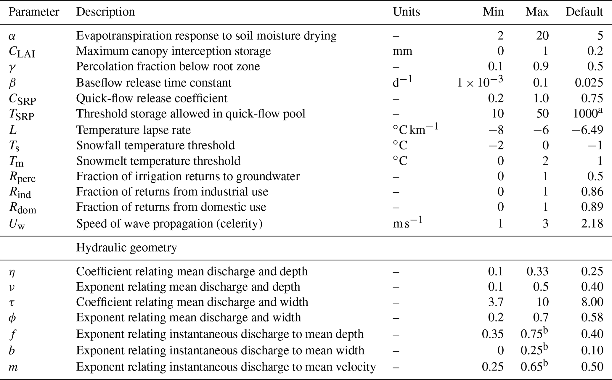
a Default value effectively defines no upper bound to storage within the surface runoff pool. b The sum of f, b, and m (and ν, ϕ, and ϵ) must equal 1.
Previous work that parameterized WBM to match historical observation used a combination of manual and automated fitting. Table 1 presents a cross section of parameters that are typically varied to control the response of WBMs in individual watersheds. Default values are typically found to be reasonable for both forested, temperate watersheds and global average conditions, but poor correspondence with observational data in some watersheds is expected when simulating large regions with default values. The WBM users should calibrate the parameters listed in Table 1 (and possibly others) for regional modeling. A complete list of parameters and inputs is provided with the model source code as a spreadsheet.
2.2.1 Land surface fluxes
Water enters the land surface – and therefore the modeling framework of the WBM – via precipitation. This precipitation can be intercepted by the vegetative canopy, collect as snow, enter soil storage, or become surface runoff. Water that enters soils in excess of the soil's field capacity infiltrates the shallow groundwater pool. Bare surfaces and vegetation collectively lose water to the atmosphere through ET.
Precipitation and snow. Precipitation is partitioned into solid (snow) and liquid (rain) portions within the WBM according to temperature thresholds. Snow accumulation and snowmelt, both expressed in terms of snow water equivalent (SWE), are also functions of temperature thresholds. These snow thresholds are fully described in Wada et al. (2012) and Grogan (2016). Accumulated snow is represented as a single layer. For regions with high-elevational gradients, a subgrid-cell binned distribution of elevations can be used to partition the grid into liquid/solid precipitation portions and snow accumulation/snowmelt portions. If subgrid elevation snow processes are not used, the same snow processes apply to the entire grid cell. The subgrid-cell elevation method described in Mishra et al. (2020) and Grogan et al. (2020) is elaborated on here. The elevation distribution of each model's grid cell is calculated from a 30 or 500 m or finer-resolution digital elevation model (DEM), resulting in binned elevation categories of ΔH vertical bands. The size of the bins is user-defined and can range from 0 to 5000 m, with a default bin ΔH size of 250 m. A temperature lapse rate, L [∘C km−1] is applied to the mean daily temperature T [∘C] at the reference elevation Href [m] for each binned elevation category, resulting in an adjusted mean temperature Te [∘C], for the portion of each grid cell in elevation bin category e.
The reference elevation Href [m] is the average elevation of the grid cell represented by the temperature dataset. Precipitation rates are assumed to be equal across all elevation bins e, such that Pe=P, where Pe [mm d−1] is the precipitation rate at elevation e, and P [mm d−1] is the input precipitation rate. The SWE in elevation bin e, Se [mm], is updated through time steps of length dt:
where the frozen precipitation rate [mm d−1] is a function of the temperature at elevation e, Te [∘C] and a reference temperature Ts [∘C]:
and calculation of snowmelt at elevation bin e, Me [mm d−1] follows the methods from Willmott et al. (1985):
The total SWE, S [mm d−1], in the grid-cell at each time step is the sum of all SWE values at each elevation band e multiplied by the corresponding fraction of grid-cell area represented by elevation bin e, fe:
Variables controlling SWE accumulation include the snowfall threshold Ts, with a default value of −1 ∘C; the snowmelt threshold Tm, with a default value of 1 ∘C; and the lapse rate L, with a default value of −6.4 ∘C km−1. Both Te and L can be constants for the whole simulation domain, or they can be a spatially variable gridded input layer.
At high elevations and cold climates, it is a common case that annual snowfall exceeds annual snowmelt volume. In reality, this excess snowpack converts to ice and forms glaciers. The WBM does not internally simulate glacier formation or dynamics; this causes unrealistic, infinite snow accumulation. To address this problem, users can define a threshold (e.g., 5000 mm of SWE) above which snow water volumes are shifted down elevation bands on the date of annual snowpack minimum (assumed to be 15 August in the Northern Hemisphere and 15 February in the Southern Hemisphere). If there is no elevation bin in the grid cell in which snow is melting, snow water is further shifted downstream to the next grid cell, following the direction of flow as defined by the digital river network.
Canopy interception. Vegetation intercepts incoming precipitation, preventing some of the total precipitation from reaching soils below and adding to the total ET flux. The canopy intercepts liquid precipitation only. The WBM uses canopy rainfall interception formulations from Deardorff (1978) and Dickinson (1984):
where Wi is canopy water storage [mm], [mm] is the canopy water storage capacity, P [mm d−1] and Pt [mm d−1] are liquid precipitation and throughfall, respectively (see “Precipitation and snow” subsection above), and Ec [mm d−1] is evaporation of the canopy water.
Canopy water storage is limited by its capacity , which is proportional to the leaf area index (LAI) [m2 m−2]:
where CLAI is canopy interception coefficient [mm] typically ranging from 0.15 to 0.25 mm (Dingman, 2002); WBM uses a default value of 0.2 mm, as suggested in Dickinson (1984).
The canopy water evaporation rate Ec [mm d−1] is a function of the canopy water storage Wi [mm], canopy water storage capacity [mm], and the open water evaporation rate Eow [mm d−1] (Deardorff, 1978):
Throughfall is then calculated as the amount of water overfilling the canopy interception pool, while accounting for evaporation over the course of the time step.
Open water and impervious surfaces. The WBM represents direct storm runoff over impervious surfaces (Zuidema et al., 2018); the latter prevents water from entering soil and increases storm runoff. If provided with a map of impervious surface fractions of the grid-cell area, the WBM assumes no soil water holding capacity and does not calculate canopy interception on those areas. To define the fraction of precipitation that is routed directly to streams, the WBM calculates an effective impervious area adapted from Alley and Veenhuis (1983):
Given an input dataset of the fraction of grid-cell open water areas fow (e.g., lakes and ponds), the WBM treats open water areas as direct contributors of storm runoff to river systems; open water grid cells have no soil infiltration, surface retention pool, or shallow groundwater pool. The WBM limits the sum of impervious surface and open water areas to 97.5 % of the grid-cell area for continuity, except for expansive lakes occupying entire grid cells which are masked from any terrestrial water balance calculations. Endorheic lake grid cells are also fully masked from terrestrial wate balance calculations; they are treated as water outlets in the same way that ocean grid cells adjacent to river mouths are outlets. Direct storm runoff Rstrm [mm d−1] is calculated as the sum of incoming precipitation P [mm d−1] and snowmelt water M [mm d−1], multiplied by the sum of the effective impervious area fraction and open water fraction fow:
Storm runoff Rstrm [mm d−1] is routed directly to streams. The remainder of precipitation and snowmelt water are routed to soil infiltration. If soil is already saturated, this remainder contributes to surface runoff and shallow groundwater recharge (see below for descriptions of these processes); Hortonian (infiltration excess) flow is not simulated.
Soil moisture balance. Soil moisture balance, WS [mm], is calculated by tracking a grid cell's water inputs, water outputs, and holding capacity of the soil moisture pool. The WBM simulates a single soil layer, and does not explicitly represent vertical fluxes of water through the soil. The soil moisture pool's available water capacity Wcap [mm], is determined by the rooting depth Rd [mm], soil field capacity Fcap [–], and soil wilting point Wpt [–]:
The WBM can take these soil and vegetation parameters – rooting depth, field capacity, and wilting point – as inputs and calculate the soil available water capacity as described in Eq. (11), or it can take available water capacity as a model input.
Water inputs to the soil come from throughfall of liquid precipitation Pt [mm d−1], and snowmelt M [mm d−1]. Output is via actual evapotranspiration, AET [mm d−1], modified by a soil-drying function g(Ws), and gravity drainage D [mm d−1]. Soil moisture balance calculations for natural land covers are fully described in Wisser et al. (2010a) and crop land covers in Grogan (2016). Change in soil moisture is calculated at each time step [d] as:
where gravity drainage D [mm d−1] is a function of the soil available water capacity Wcap [mm], actual evapotranspiration, AET [mm d−1], throughfall of liquid precipitation Pt [mm d−1], snowmelt M [mm d−1], and the water depth stored in the soil moisture pool in the previous time step:
This gravity drainage water becomes surface runoff and/or recharge to the shallow groundwater storage pool.
Potential and actual evapotranspiration. Evaluation of different potential evapotranspiration (PET) functions is provided in Vörösmarty et al. (1998); the version of WBM described here has options to use the Hamon (1963), Penman–Monteith (Penman, 1948; Monteith, 1965), and FAO Irrigation and Drainage Paper No. 56 modification to Penman–Monteith (Allen et al., 1998) PET functions. The Hamon method requires only two climate inputs (temperature and precipitation), while the other two functions require additional inputs of air humidity (relative, absolute, or dew/wet-bulb temperature), wind speed vectors, and cloud cover. The Hamon and Penman–Monteith functions are both described in Vörösmarty et al. (1998), and the FAO Irrigation and Drainage Paper No. 56 (Allen et al., 1998) modification to Penman–Monteith PET is described in the WBM model documentation provided in the Supplement.
Actual evapotranspiration (AET) from naturally vegetated land areas is a function of the PET, soil moisture, and soil properties; these soil properties are field capacity, wilting point, and rooting depth (see Eq. 11 above). In a given time step, if soil moisture is sufficient to meet PET, then AET = PET. Otherwise, PET is modified by a soil-drying function g(Ws). The amount of water that can be drawn out of the soil moisture pool depends on the current soil moisture and the available water capacity. These functions are described fully in Wisser et al. (2010a) and Grogan (2016). Default model inputs represent the land surface as a generic, reference vegetation type (Allen et al., 1998), with soil-drying parameters from Federer et al. (2003) estimated to best match global average runoff. The ET from land-cover types other than a generic reference vegetation can be represented, given input data on the subgrid-cell fraction occupied by these land-cover types and a set of associated parameters. When using subgrid-cell land-cover inputs, the WBM simulates a full soil water balance for each portion of the grid cell that is identified as a unique land-cover type. Model output provides a grid-averaged value for each stock and flux. For cropland land-cover inputs, subgrid-cell crop-specific water balance values can be output for soil moisture, PET, irrigation water applied (for irrigated crops), and blue and green water use by crop (for irrigated crops). For fine-resolution simulations, inputs identifying the dominant land-cover type can be used to parameterize the entire grid cell, or land cover can be used to average necessary parameters a priori. Crop ET calculation methods are from Allen et al. (1998), with default parameter values for crops from Siebert and Döll (2010). While AET from other land-cover types (e.g., forest or grassland) can be parameterized and simulated, no published study has used this option of WBM yet. The AET from other consumptive water uses are described below in Sect. 2.2.5.
Open water evaporation applies to the fraction of grid cells containing terrestrial free water surfaces, including river surface area, lake and reservoir area, and inter-basin transfer canal area (see Sect. 2.3.4 below for a description of inter-basin transfer canals). Open water evaporation rates can be input into the WBM, available from reanalysis models such as MERRA2 (Gelaro et al., 2017), estimated as a multiplier on PET in the absence of an input dataset; the default multiplier in the WBM is 1.0. The river surface evaporation Eriv is calculated as a function of open water evaporation rates O and river geometry:
where A is the grid cell area [m2], yR is the stream width [m], Eow is the open water evaporation rate [m d−1], and WR is the storage of water in the river [m3]. Hydraulic geometry relations used to estimate stream width are described below in Sect. 2.2.3.
Surface runoff. When water enters a grid cell in excess of the volume that can be stored in soils, the canopy, and lost through ET, then gravity drainage occurs, resulting in both surface runoff and recharge. The distribution of this excess water between surface runoff and shallow groundwater recharge is defined by a model parameter which sets the fraction of drainage water that recharges shallow groundwater; the complement of this value is treated as surface runoff. To capture the hydrodynamic response of runoff generation following precipitation and snowmelt events, water passes through either a surface retention pool or a shallow groundwater pool, described below. Once the runoff water leaves either of these pools, it joins with storm runoff and forms total land runoff that is then routed downstream as river flow.
Surface runoff, RS [mm d−1], is retained in the surface runoff retention pool, WSRP [mm], prior to draining to the stream network. This temporary storage of surface runoff in the surface retention pool represents flow over the land surface and temporary storage in ephemeral pools and wetlands. The drainage rate, RSRP [mm d−1], from the surface runoff retention pool, WSRP [mm], follows a tank drainage formulation:
where CSRP is a unitless discharge coefficient of the surface runoff retention pool and includes unit conversions, and G is gravitational acceleration.
There is an upper limit, TSRP [mm], imposed on the storage volume in the surface runoff retention pool. This limit captures the response of over-filled surface topographic depressions. When the volume of the surface runoff retention pool exceeds this limit, then the overflow water, REXC [mm d−1], is moved to the river. This helps to capture flashy hydrodynamic responses more accurately during extreme events (Zuidema et al., 2020). Change to the storage value of the surface runoff retention pool WSRP is as follows:
where RS [mm d−1] is surface runoff, RSRP [mm d−1] is the drainage rate out of the surface runoff retention pool, tE are times when the surface runoff pool exceeds the limit, δ represents the Dirac delta, the integral of which over 1 time step equals unity, and REXC [mm d−1] is the overflow water.
The balance of the surface runoff retention pool is calculated as a split operator in three stages:
-
-
where
-
where
where and are the storage in the surface retention storage pool at the previous and present time step, respectively. The threshold for storage in the surface runoff retention pool (TSRP) is set to 1000 mm by default, which effectively turns off this functionality, unless an alternate value is defined. Decreasing TSRP to values in the range of 15 to 50 mm increases the flashy response of the model in temperate climates, enabling users to calibrate this parameter to capture regional variations in storm responses.
Glacier runoff. Another flux of water from the land surface to the rivers is glacier runoff. While the WBM does not simulate glacier formation and dynamics beyond routing the accumulated snowpack downstream as described above, it can take inputs of glacier area and runoff generated on that area. The glacier area within each grid cell is removed from the land area simulated by the WBM; all water accumulation and runoff from that land area is taken from the glacier input dataset. The WBM assumes that this land area, which is typically a fraction of a grid cell, sits at the highest elevation within the grid. To avoid double-counting precipitation inputs onto this land area (which is accounted for by the glacier input dataset), the WBM reduces grid-cell precipitation linearly by the fraction of the grid cell covered by glacier area. Each glacier has a single designated outlet location, even in the case that the full glacier covers multiple grid cells, and it is also assumed that runoff from the glacier area all flows directly into the outlet grid cell's river system. These methods are first described in Mishra et al. (2020), and were developed to make use of rasterized output from the Python Glacier Evolution Model (PyGEM; Rounce et al., 2020a), which provides glacier runoff at a monthly time step. The standard output format of PyGEM is not gridded; rather, post-processed PyGEM output is required as input for the WBM (Prusevich et al., 2021).
2.2.2 Groundwater
Shallow groundwater storage pool. As noted above, when water enters a grid cell in excess of the volume that can be stored in soils, the canopy, and lost via ET, then runoff and recharge both occur. The portion of that excess water that becomes recharge is defined by the recharge fraction parameter, with a default value of 0.5. Alternative non-default input values can be a constant applied to the whole simulation domain, or a gridded layer to reflect its spatial variability. The recharge water enters a below-soil storage pool called the shallow groundwater storage pool. This shallow groundwater pool generates baseflow (i.e., subsurface runoff) by leaking water to the river system stream reaches in the same grid cell where recharge occurred. The leakage rate, RSGW [mm d−1], is a function of a hydrodynamic groundwater constant, β [d−1], applied to the depth of water stored in the shallow groundwater pool, WSGW [mm]:
The default value for β is 0.025.
Unsustainable groundwater. Following the GHM methods of Hanasaki et al. (2008a) and Wada et al. (2012), the WBM additionally represents an unsustainable groundwater source. The WBM's implementation of unsustainable groundwater was first described in Wisser et al. (2010a), and again in Grogan et al. (2015, 2017), Liu et al. (2017), and Zaveri et al. (2016). Here, as in previous WBM and other GHM publications, unsustainable groundwater is defined as groundwater used in excess of the recharge stored in the shallow groundwater pool. We acknowledge that this definition does not capture the complex nature of surface water–groundwater interactions; however, this definition has been adopted by the GHM community as sufficient for macro-scale representations of the large volumes of water required to meet agricultural water uses that are clearly in excess of surface water and short-term (yearly to decadal) groundwater recharge supplies (Hanasaki et al., 2008b; Wada et al., 2012; Grogan et al., 2017; Hanasaki et al., 2018). The unsustainable groundwater source is not defined as a stock or storage pool, hence no state variable is associated with it. When the demand for water extractions (see Sect. 2.2.5 below) exceeds the water supply available from surface water and shallow groundwater, the WBM has the option of allowing the residual, or a parameter-defined fraction of the residual, to be supplied from an unlimited unsustainable groundwater source. This effectively defines unsustainable groundwater use – alternatively known as groundwater mining or the use of fossil groundwater when recharge is known to have occurred pre-historically (Jasechko et al., 2017) – as any groundwater extraction in excess of the long-term recharge rates applied to the shallow groundwater pool and represents an additional source of water entering the simulated hydrologic system. Prior work (e.g., Gleeson et al., 2012; Grogan et al., 2015, 2017; Wada et al., 2012; Zaveri et al., 2016) has shown that the assumption that this unsustainable water source is available is reasonable at a macro-scale and allows GHMs to evaluate aquifer mining at large scales and compare to groundwater-based mass change observations from the GRACE satellite (Sutanudjaja et al., 2018).
2.2.3 River discharge
The WBM has a horizontal water transport model that represents the flow of rivers in one dimension. The foundation of this model is the digital river network, which defines exactly one flow direction for each grid cell. As grid cells connect into networks, these form the representation of river systems. Note that every grid cell has a flow direction, regardless of whether enough water accumulates to actually flow through the grid cell or not (e.g., an arid region with no or low precipitation would have no flow, but would have a defined network of flow directions, as described by the STN-30p network (Vörösmarty et al., 2000b). The model offers two options for calculating river flow velocity: (1) a Muskingum-Cunge solution of the Saint-Venant flow equations (Maidment, 1993), and (2) a linear reservoir routing solution. We find that the Saint-Venant flow equations are only appropriate for simulations of relatively coarse grid-cell resolution – half-degree by half-degree or larger – where much of the river's volume remains within the grid cell over a 24 h time period. For the finer-resolution simulations – 5 min grid-cell size and smaller – that are now common amongst many GHMs, the linear reservoir routing method is more appropriate. The Muskingum-Cunge solution is fully documented in Wisser et al. (2010a) and Grogan (2016), and the linear reservoir routing method follows common formulations (Dingman, 2002, p. 429). Linear reservoir routing calculates reach outflow as a function of the water volume within each grid cell, with a release coefficient that is a function of celerity (rapidity of downstream motion) and reach length. Both methods are described again in the model documentation in the Supplement.
Hydraulic geometry. The WBM incorporates both downstream and at-a-station stream geometry relationship assumptions to calculate river width, depth, and velocity from discharge. The WBM assumes that each grid cell has a single representative stream reach and calculates a rolling average of annual mean discharge for each reach in a simulation over the previous 5 years of a simulation. The long-term mean discharge, [m3 s−1], is then used to estimate the long-term mean depth, [m], width, [m], and velocity, [m s−1], using downstream hydraulic geometry relations and scaling factors from Park (1977):
where η, ν, τ, ϕ, δ, and ϵ are user-defined variables, with optional default values listed in Table 1.
Instantaneous estimates of the three variables (z [m], y [m], and u [m s−1] for depth, width, and velocity, respectively) are given as functions of instantaneous Q [m3 s−1] and mean discharge [m3 s−1], scaled by appropriate at-a-station hydraulic geometry exponents (Dingman, 2009):
In the above equations, parameters f, b and m are all user defined variables, with optional default values from Leopold and Maddock (1953), listed in Table 1.
2.2.4 Hydro-infrastructure
Dams and reservoirs. Large dams and reservoirs alter river flows and provide water supplies to surrounding areas. When provided with a database containing the required information, WBM simulates the impact of reservoir operations on river flow, and it uses the water stored in reservoirs as supply for water extractions and consumptive uses (see Section 2.2.5 below). The input dam database must have the following information to be of use to WBM: the year of dam construction, the reservoir area and capacity, the upstream catchment area, the main purpose, and the location. The database may optionally include information about the year a dam was removed, if applicable. Dam databases with this information include the Global Reservoir and Dam Database (GRanD; Lehner et al., 2011), and the Hydrologically Consistent Dams Database (HydroConDams; Zuidema and Morrison, 2020).
The WBM employs a general reservoir water release rule, with parameter modifications for dams of different purposes, such as irrigation supply or flood control. A general water release rule is designed to maintain outflows approximately equal to average annual inflows, but to release less water when reservoir levels are low and more water when reservoir levels are high. Water levels that are considered “high” or “low” are based on the purpose of the dam and can be parameterized for specific dams or set of dams. Dams on irrigation reservoirs are additionally parameterized with a time series of downstream irrigation water requirements, ensuring that water is released downstream from the dam during the time of greatest water extraction demand. In reality, many irrigation reservoirs are connected to downstream irrigated areas by canal systems that flow directly from the reservoir and do not rely on dam operations. The WBM does not represent these canal systems, and thus uses dam water releases to account for this canal-enabled downstream flow of water. Full reservoir release methods, along with parameter values assigned to different dam types, are documented in Rougé et al. (2021). Alternatively, discharge from individual dams can be input directly into the WBM, thereby making calculated reservoir storage a function of observed reservoir output (Zuidema et al., 2020); this ensures that releases match historical records in cases where WBM's default functions vary too far from observed reservoir operations.
Reservoirs with a storage capacity below a given threshold (default is 1 km3) are treated as unmanaged spillway dams with the spill gate geometry determined from the stream geometry for the average annual flow. Water release from these structures are calculated from the hydraulic formulations for those dam structures given in the US Army Corps Engineers handbook (United States Bureau of Reclamation, 1987; US Army Corps of Engineers, 1987). Natural lakes are treated in a similar way as the spillway dams, but the gate geometry is determined as those from instantaneous riverbed geometry described above.
Small irrigation reservoirs. Rainwater harvesting for irrigation water supply is represented in the WBM's small irrigation reservoir module. These small reservoirs do not dam rivers as larger reservoirs do, and hence do not alter river flow. Rather, they collect rainwater and surface runoff, storing it on the land surface and preventing it from reaching the river system. Note, these are not run-of-river reservoirs, but structures on the land surface. We do not know of any global or even regional dataset that describes the location and capacity of these small irrigation reservoirs. Small irrigation reservoir methods of the WBM were first developed and described in Wisser et al. (2010b), where a range of capacities were simulated to provide a sensitivity analysis and quantify the potential importance of these highly localized water supply systems.
Inter-basin transfers. Inter-basins transfers are large canals, tunnels, or pipelines that move water across river basin boundaries. These large projects alter flows in both the sending and receiving river systems and can be used to supply water for consumptive uses. The WBM simulates how inter-basin transfers alter the flows in both the sending and receiving rivers, though it does not explicitly represent the routing of water discharge through the canal system. The WBM's inter-basin transfer methods were first developed and described in Zaveri et al. (2016) and described again in Liu et al. (2017). Five parameters are used to simulate the water transfer: (1) the water sending point latitude and longitude, (2) the water recipient latitude and longitude, (3) a minimum allowed sending river flow, (4) a maximum allowed canal intake flow, and (5) a water release rule for flow volumes between the minimum and maximum. A database of India's inter-basin transfers was used by the WBM in Zaveri et al. (2016) and is included as a Supplement to that publication.
2.2.5 Water extraction and consumptive water use
Water extractions from rivers, reservoirs, and groundwater are an important part of simulating water supply and changes in human–hydrologic interactions. The WBM first implemented water extractions for irrigated agriculture (Wisser et al., 2008, 2010a), which is globally known to account for ∼70 % of all freshwater extractions (Rosegrant and Cai, 2002). Modules for water supply to livestock, domestic, and industrial use, which are less consumptive than irrigation water and account for a smaller proportion of total global extractions, were added to the WBM in Liu et al. (2017). When water is removed from a storage (e.g., reservoirs or the shallow groundwater pool), the storage value of that stock is updated within the daily time step.
Water withdrawals are taken from different water stocks and fluxes based on a given priority order of both water users and water sources; this rule set has a number of user input options and parameters, making it highly flexible and customizable. The default priority order for withdrawal by water users within a grid cell is as follows: (1) domestic, (2) industrial, (3) livestock, and (4) irrigation. In turn, the withdrawals from each user group come from water storage and flux pools in the following order until the requested withdrawal water volume is met:
-
Small irrigation reservoirs – source is available only to livestock and irrigation water use
-
Shallow groundwater (SGW) – when SGW is extracted for domestic, industrial, and livestock use, all the water in the SGW pool can be extracted, up to the volume requested by the sector. When this source is extracted for irrigation, an optional parameter, rsg [–], defines the target ratio of groundwater-to-total withdrawals for irrigation water extractions. This parameter can be a constant or a spatially variable grid. If rsg is not defined, all available SGW is extracted for use (up to the water demand) in this step. In the case where rsg is defined, this first groundwater withdrawal step takes water from SGW up to the volume defined by the product of rsgw and irrigation water demand, D [mm], even if there is more SGW available and D is greater than the defined water amount, such that shallow groundwater withdrawal, Wsgw, at this step is
-
Surface water in a river or reservoir within the same grid cell – stream water available for extraction, Se, is the sum of water retained in river and reservoir storage at the end of the previous time step, Wk−1, and the volume of water flowing through the reach during the previous time step, Qk−1, limited by a scaling factor that is set to the default value of 0.8:
The scaling factor of 0.8 prevents river reaches from being completely dried out by water extractions;
-
Shallow groundwater – second extraction for irrigation only. If the parameter rsgw is defined in a way that limited SGW extraction for irrigation to less than the available SGW volume in Step 2, and there is still residual water demand, then water volumes up to the remainder of the SGW storage volume can be extracted at Step 4. By combining Steps 2 and 4, the target irrigation groundwater-to-total withdrawal ratio is achieved only in the case where the sum of surface and SGW volumes is sufficient to meet this ratio; Step 4 ensures that fulfilling water withdrawal demands using sustainable resources within the grid cell takes priority over achieving the target ratio. This step does not apply to livestock, domestic, or industrial water extractions, as no ratio parameter is applied to those water uses;
-
Surface water in a river or reservoir outside the given grid cell that has the largest storage + discharge volume within a set of parameter-defined radii – a different parameter can be set for irrigation water use than for other uses, representing the differences in irrigation and municipal water supply infrastructure. The default radius value is 100 km for all water uses; the user can define a set of alternative constant scalars or gridded layers of values;
-
Unsustainable groundwater (UGW) – water available for extraction from this pool may be limited by the UGW allowance ratio, if defined. Because this source of water has no stock value, the allowance ratio applies a scaling factor of ≤1 to the water withdrawal demand. This scaling factor is independent of rsgw, and if not defined, this pool is unlimited.
Irrigation. Given inputs of irrigated land area and associated crop-specific parameters, the WBM calculates the agronomic water requirements for optimal crop growth over its three growing seasons: (1) planting and development, (2) growth, and (3) harvesting. In the WBM, crops extract water from the soil moisture pool each day of the crop's growing season. Given sufficient water in the soil moisture pool, the amount of water used by each crop is the crop's PET. When soil moisture levels drop below a crop-specific threshold, the difference between the soil moisture level and field capacity is defined as the irrigation water requirement. This method of crop irrigation water requirements follows FAO guidance (Allen et al., 1998), as is typical of GHMs. The WBM's crop irrigation water requirement methods have been described in Grogan et al. (2015, 2017), Liu et al. (2017), Wisser et al. (2010a), Zaveri et al. (2016) and Zuidema et al. (2020).
Alternatively, the WBM has the option to calculate a daily crop gross irrigation water requirement instead of using the crop-specific soil moisture threshold to trigger water extractions. This option is useful for simulations with large grid-cell sizes, where the calculation of average soil moisture over large irrigated areas leads to unrealistically high irrigation water demands in a single day. When using this option, the WBM estimates gross crop irrigation water requirements each day, equal to the difference between soil moisture content and field capacity, and modified by either the classical irrigation efficiency parameter or the irrigation technology-derived classical efficiency for the day (described below). Irrigation water is then extracted from water sources each day, and stored in an irrigation water storage pool that does not interact with other fluxes within the model until the day when the crop-specific soil moisture threshold is reached. When this threshold is reached, water is moved from the irrigation water storage pool to soil moisture. This option extracts relatively small amounts of water from water stocks each day, instead of larger amounts of water on the day that the soil moisture threshold is reached. These smaller, daily extractions may better simulate the temporal distribution of irrigation activity over large grid-cell areas.
The amount of water required by a crop to achieve AET = PET is less than the amount of water that must be extracted from a water source due to inefficiencies in irrigation water extraction, transportation, and application. The WBM has two options for calculating the gross irrigation water extraction required as a function of net irrigation water required by the crop: (1) the irrigation efficiency method, and (2) the irrigation technology method. In both cases, water extracted in excess of net irrigation water requirements are returned to surface and groundwater systems on the same day as extraction. Returns to the surface water system are treated as surface runoff (see above description of surface runoff), and are added to the surface runoff storage pool. Returns to the shallow groundwater system are treated as shallow groundwater recharge (see above).
The irrigation efficiency method is standard for GHMs and described in Grogan et al. (2015, 2017), Liu et al. (2017), Wisser et al. (2010a), and Zaveri et al. (2016). In this method, classical irrigation efficiency is an input to the WBM and directly modifies the net irrigation water requirement by a spatially varying constant. Classical irrigation efficiency is defined as the ratio between net irrigation water required and gross water extractions. Net irrigation water requirements include water transpired by the crops and associated soil evaporation that is unavoidable. As described in Grogan (2016) and Wisser et al. (2010a), net irrigation water requirements for rice paddies also include an additional water volume, representing the water needed to enable flooding at the start of the growing season and maintenance of the flood paddy water level throughout the season to compensate for percolation. The volume of water added to initially flood the rice paddies is an input parameter with a default depth value of 50 mm applied over all irrigated rice paddy areas. The daily additional water application rate used to maintain the paddy depth is based on the rate of water percolation through the underlying soils. This is also an input dataset, with methods for calculating percolation rates from soil property data described in Wisser et al. (2010a). Both the initial paddy flood water and the daily maintenance water are included in net irrigation water volume of the irrigated rice, and the irrigation efficiency parameter is applied to these volumes in the same way it is applied to other net irrigation water requirements.
The irrigation technology method in the WBM is first described in Zuidema et al. (2020); it represents non-consumptive irrigation water losses as a function of irrigation technology-specific parameters and open water evaporation rates (which can be input or calculated as a function of weather inputs). In this second method, inputs on the spatial distribution of different irrigation water conveyance and application technologies (Jägermeyr et al., 2015, 2016) is required, and the inefficient water losses that occur over space and time are calculated within the WBM as a function of irrigation technology type and weather variables. Therefore, classical irrigation efficiency is calculated and provided as a time- and space-varying model output.
Blue water and green water use for irrigation. Falkenmark and Rockström (2006) introduced the concept of “blue water” and “green water” into the GHM literature to distinguish between direct precipitation and irrigation water sources in crop AET. Blue water is defined as liquid water that can be extracted from aquifers, surface water reservoirs (lakes and dams), and river systems, and green water is defined as soil moisture water originating from direct precipitation (including snowmelt) (Falkenmark and Rockström, 2006). The WBM can estimate the flux of blue and green water via ET by irrigated crops. Note that all ET from rainfed crops is by definition green water. All water that becomes irrigated crop ET must first enter the soil moisture pool. Water enters the soil moisture pool by either (1) direct precipitation or snowmelt, which is green water, or (2) irrigation from surface or groundwater, which is blue water. We assume that water in the soil moisture pool is well mixed on a daily time step. Therefore, the ET out of that pool has the same proportions of blue and green water as the soil moisture pool itself. Optional model output variables include the grid-cell average soil moisture that is made up of blue and green water [mm], grid-cell total ET of blue and green water from the soil storage pool [mm d−1], crop-area specific soil moisture values of blue and green water [mm] (e.g., blue water stored in soils under a specified input crop type), and crop-specific ET of blue and green water [mm d−1].
Table 2Default livestock parameters for the livestock water use module.
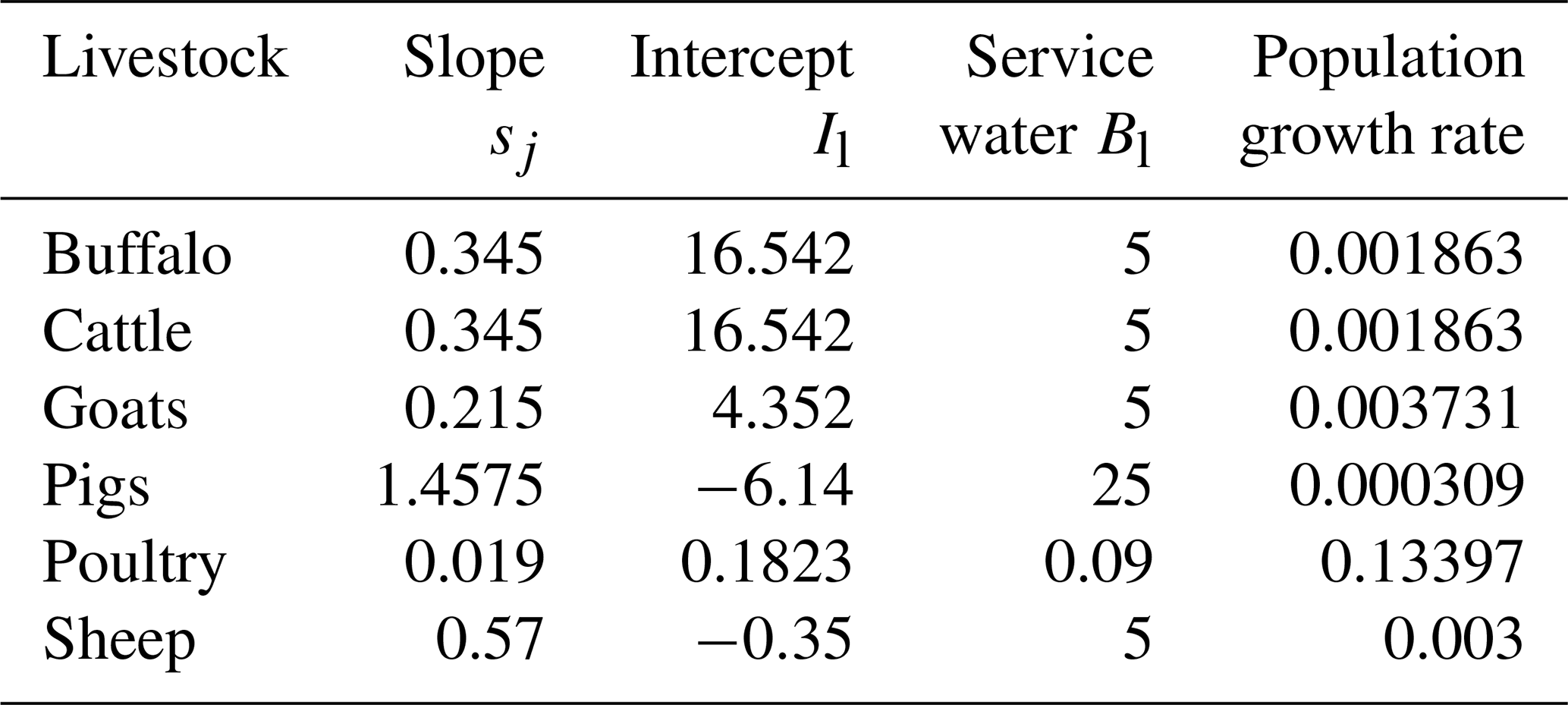
Livestock. Livestock require water for drinking and for service water, which includes washing and cooling. The WBM uses the methods and default parameter values (Table 2) provided by Steinfeld et al. (2006) to calculate livestock water use by animal type. Daily livestock water, Lw [m3 d−1], for each livestock type is calculated each day as
where Il [m3/head/day] is the minimum water demand for livestock type l, sl [m3/head/∘C/day] is the temperature-induced consumption requirement for livestock type l [–], T is the daily mean air temperature, with a minimum value of 0 [∘C]; Bl [m3/head/day] is the daily service water volume required per animal, and Dl is the density of livestock type l in the grid cell [animal head/grid cell]. Additionally, an animal population growth rate can be applied to each livestock head density category to represent increases in population over a given single-year value of animal head density data (the year of Dl, input reference livestock density). This is useful as limited global livestock density data are available. Livestock are assumed to consume 5 % of their water extractions, with the remaining 95 % returning to the system via runoff; the ratio of consumption to return flows can be modified by user-defined input parameters.
Domestic and industrial. Households and industry extract water for a range of purposes, and at rates that have great spatial variability. The WBM represents these extractions based entirely on an input per capita water extraction rate and a population density map, such that domestic water use, Ud [m3/grid cell/day], is
and industrial water use, Ui [m3/grid cell/day] is
where A [km2] is the area of the grid cell, udom [m3/person/day] is the per capita domestic water withdrawal, uind [m3/person/day] is the per capita industrial water use, andDpop [persons/km2] is the population density. Domestic and industrial water use each have unique return-fraction coefficients, which default to uniform values of 84 % and 89 %, respectively.
2.2.6 In-stream nitrogen and water temperature
Nitrate–nitrogen concentration. The WBM estimates in-stream and in-reservoir nitrate–nitrogen (N–NO3) concentration. In-stream N–NO3 concentrations are a function of point-source nitrate inputs from wastewater treatment plants, nonpoint-source nitrate inputs from the land surface, and in-stream denitrification. Wastewater treatment plant contributions to in-stream nitrate are calculated using data on served population and waste treatment type, as described in Samal et al. (2017). Nitrate inputs from land are estimated as a function of simulated grid-cell runoff and the estimated nitrate concentration in runoff from different land-use types. Estimation of land use-specific runoff nitrate concentrations are described in Wollheim et al. (2008a). The suite of parameters describing nitrate concentration in runoff from different land-use types may require region-specific calibration, based on high spatial resolution nitrate sampling from headwater catchments along a gradient of human land use and flow conditions (Wollheim et al., 2008a). The model default values are found to be adequate for moderately developed landscapes with modest agricultural cover in the northeastern United States (Samal et al., 2017; Simon, 2018; Stewart et al., 2011). In-stream (Stewart et al., 2011) and in-reservoir (Simon, 2018) denitrification are calculated using temperature-corrected denitrification along the benthic surface assuming efficiency loss kinetics, following Mulholland et al. (2008) and Wollheim et al. (2014).
Water temperature. River temperature is calculated following Stewart et al. (2013) with an addition to account for air humidity and canopy shading (see documentation in the Supplement for details). Temperature is first calculated on the landscape, mixing air temperatures depending on the timing of shallow groundwater recharge. River temperature re-equilibration is then calculated through a combined empirical and deterministic re-equilibration procedure given by Dingman (1972). The re-equilibration is a function of channel hydraulics, air temperature, solar radiation, humidity, and wind speed.
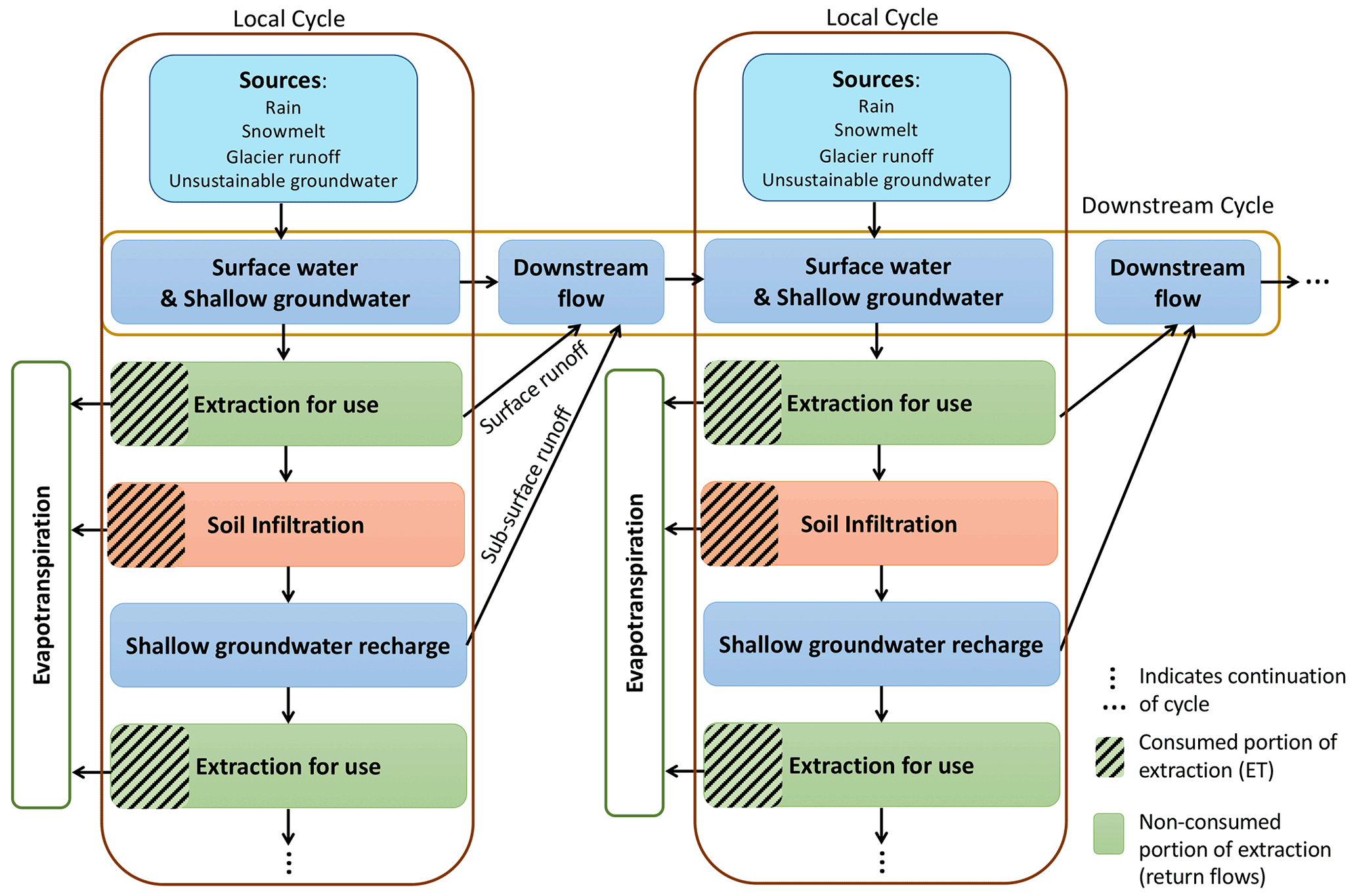
Figure 2Schematic representation of the primary source component tracking. All surface water and shallow groundwater are composed of the four primary sources: rain, snowmelt, glacier runoff, and unsustainable groundwater. When surface water and/or shallow groundwater is extracted for use, this initiates both a local cycle and a downstream cycle of water use and re-use. In the example shown here, water is extracted and applied to soils (irrigation). A portion of the extracted water and a portion of the soil water become evapotranspiration (the consumed portion, shown with hashes). Some of the water applied to soils percolates to the shallow groundwater pool. Water from the shallow groundwater pool can be extracted again, continuing the local water re-use cycle. Water extracted for use, and water from the shallow groundwater pool, generate runoff that moves downstream. This initiates a downstream cycle in which this water can be re-extracted for use from the surface water system. Downstream cycles intersect with local cycles, as water from the four primary sources are input into every locality. Figure modified from Grogan et al. (2017).
2.2.7 Water source tracking
The WBM tracks water from each source (water inputs into each individual grid cell) through all flows and stocks within the model. Stocks within each grid cell include soil moisture, small reservoir storage, shallow groundwater storage, surface retention and irrigation storage pools, rice paddy flood waters, river storage, and large reservoirs. Flows are infiltration into soils, surface runoff, recharge to shallow groundwater, baseflow, river discharge, water discharge from reservoirs, evaporation, ET, inter-basin transfers, water extracted for human water use, and return flows from human water use. These stocks and flows are depicted in Fig. 2. The WBM's tracking functionality retains information about the generative mechanism (i.e., the water source) as water flows across the landscape through the river network. This includes processes such as extraction for human use, and subsequent redistribution according to hydrologic flow paths.
The same tracking algorithm applies to all water source components. For any water component c in water storage stock S at time step k in a given grid cell,
where is the fraction of stock S composed of component c at time k. The total volume of stock S at time k is Sk; Ii are inflows to and Oj are outflows from stock S, with Ic,i being the fractions of the ith flow composed of component c, all at time step k. Component stocks () are updated throughout the time step, such that the solution is split into multiple operators as the various fluxes impact each stock.
Table 3Tracking component categories, and the identification of the water source components tracked.
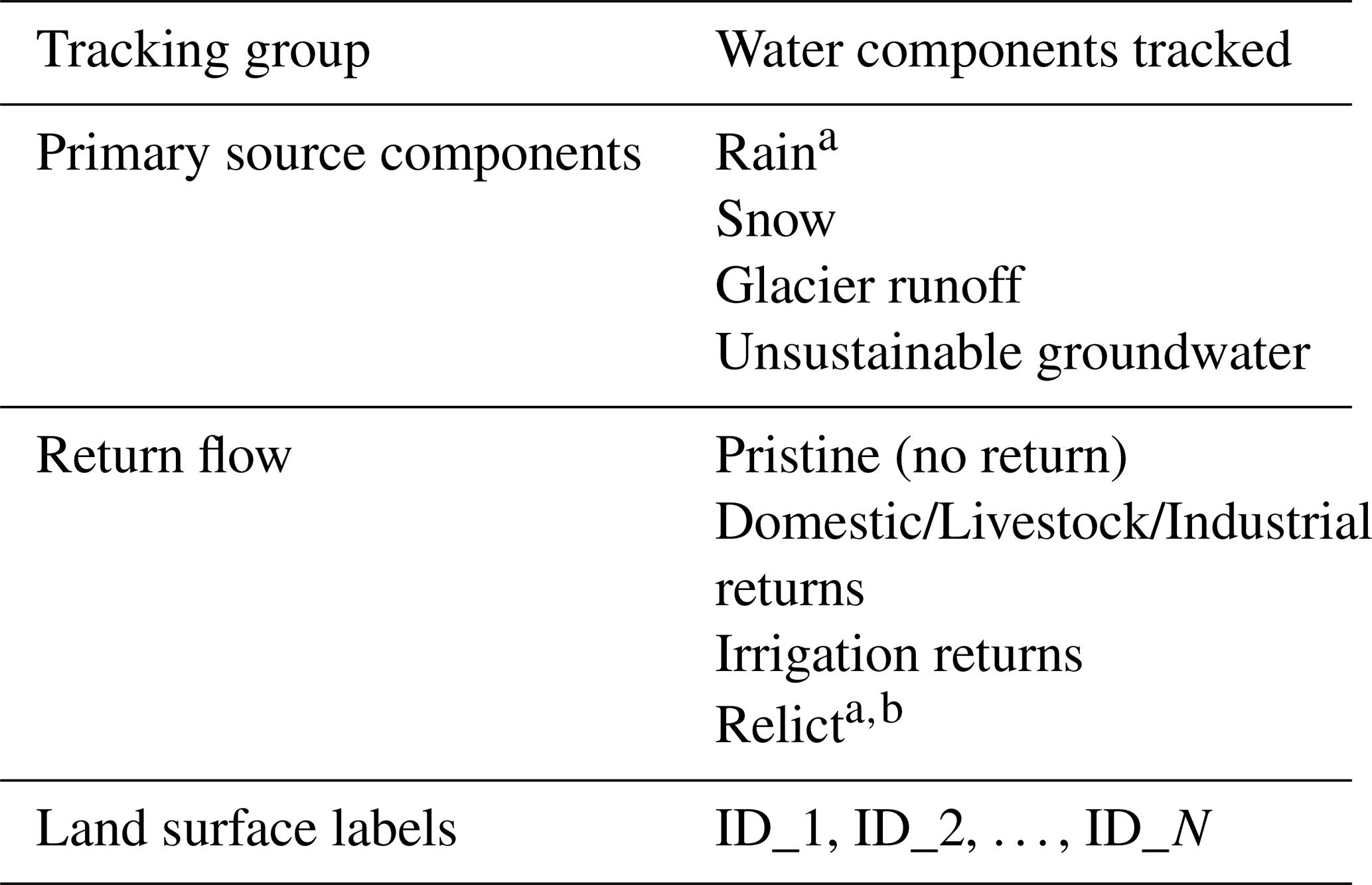
a This component comprises 100 % of reservoir and soil moisture stocks
prior to spinup
b Relict water is defined as water stored in all water storage pools
(aka stocks) at the beginning or end of spinup.
The WBM performs three types of component tracking: (1) primary source component tracking (Fig. 2), representing the initial input of water into the water balance equations, (2) return flow component tracking representing water that has been reintroduced to the hydrologic cycle following human extraction, and (3) runoff from labeled land attributes (Table 3). The model user can choose any combination of sources to track simultaneously, as the tracking modules are independent and each can be turned on or off in a given model simulation. A user interested in understanding the role of snowmelt as a component of streamflow downstream of a mountainous region would use primary source component tracking, whereas a user interested in understanding the potential for anthropogenic contaminants to be present in streamflow would use return flow component tracking. If a user was interested in runoff generated within any political boundary, land attribute tracking could be used. The intersection of different tracking components is not calculated; by turning on both primary source and return flow component tracking, for example, the WBM will not calculate the fraction of irrigation return flow composed of snowmelt. Primary source components were first described in Grogan et al. (2017), where only the unsustainable groundwater component was analyzed. Return flow components were first described in Zuidema et al. (2020); land-cover mask components are described here.
All stocks and flows are considered well-mixed so that the flows out of a stock have the same fractional water source components as the stock itself. For each tracking group (see Table 3), all stocks are initialized with Sc=1 for a given component of each group. For example, in primary source component tracking, all stocks are initialized as 100 % rain water; as the model goes through a spin-up stage, water from the other components are added to these stocks. At the beginning of a simulation, large reservoirs are initialized at 80 % of their full capacity, the soil moisture storage pool is initialized at 50 % capacity, and all other stocks begin at 0 % capacity. We recommend a minimum spin-up time of 10 years to allow all stocks to reach equilibrium storage, and importantly for many stocks to accumulate the different tracked water components. The WBM operates at a daily time step, and for some stocks (e.g., river discharge) our well-mixed assumption is appropriate; however, other stocks are typically not well-mixed at the daily time scale; for example, reservoirs (Håkanson, 2005) and groundwater (Hrachowitz et al., 2013) are known to mix at longer time scales. Therefore, we consider these fluxes with caution at short time scales (days to years), but find them informative when averaged over long periods (years to decades).
Return flow tracking has an additional option for resetting the stock component values after spinup has completed. At the end of spinup (prior to the simulation period), stocks can be reset to 100 % relict water. Relict water is defined as any water stored in simulated water stocks at the end of spinup; it makes no assumptions about the source, age, or use condition of the water. This option allows the user to interpret changes to stock components that only occur within the simulation period, removing assumptions about starting compositions. New water entering the system during the simulation period as precipitation or glacier runoff is tagged as “pristine” water. This option is one way to explicitly track the fate of components that enter the simulation at the onset of the representative simulation period (Zuidema et al., 2020).
Note that the land surface label tracking can track multiple land labels at once that can include sets of political boundaries, land-cover types, soil types, biogeographic or climate zones, or other identifiers such as the grid-cell Strahler stream order or distance of a grid cell from the river mouth. These land labels can occupy entire grid cells, or be provided as a set of grid-cell fractional coverage (i.e., a percentage of each grid cell is covered by each label type). The WBM will track each identified land label with a unique numerical ID input via a raster-based mask of unique values.
River discharge is the observational data against which most GHMs are validated, in part due to the abundance of high-quality global river discharge data and in part due to the fact that river flow is an integrative result of all the land surface fluxes simulated by GHMs. Here, we first summarize published validation of the WBM output in recent relevant papers (Sect. 3.1). We note where these evaluations make use of prior code branches (e.g., the C++ version of WBM, or FrAMES) or are regionally specific. We then present an evaluation of global river discharge, simulated by the open source WBM v.1.0.0 described here (Sect. 3.2). Furthermore, we evaluate the model's estimation of water extraction for irrigation against the only global dataset available for this metric.
3.1 Published WBM validation and evaluation
This section reviews the literature of WBM publications that include validation and/or evaluation of model components that are included in the WBM open source model. These papers report a variety of different evaluation metrics, which we summarize here.
Global river discharge. The Perl/Perl Data Language (PDL) version of WBM (described here) was most recently evaluated against global discharge from the Global Runoff Data Center reference dataset (The Global Runoff Data Centre, 2015) in Grogan (2016). Grogan (2016) reports that a linear regression of modeled versus observed average annual river discharge for the years 1980–2009 typically shows strong agreement (r2 values between 0.74 and 0.87), but that this agreement varies with the choice of input climate dataset. In comparing four different climate input datasets, the UDEL (Willmott and Matsuura, 2001) and NCEP (Saha et al., 2014) climate inputs were found to provide the best global discharge simulations, with more than 40 % of all GRDC stations achieving a Nash–Sutcliffe efficiency (NSE; Nash and Sutcliffe, 1970), a typical hydrologic evaluation metric, of >0, meaning that the model predicted observations better than the mean of historical observations. There is also spatial variation in model performance. As can be seen in Grogan (2016), river discharge from the WBM matches observations best in temperate and tropical regions, but performs poorly in arid climates. Spatial variation in validation metrics is also in part due to the choice of climate inputs. Overall, the WBM simulations from Grogan (2016) are biased low compared to observations. These results are consistent with global river discharge evaluation of the WBM's C++ version (also called WBMplus) in Wisser et al. (2010a), who report an average model mean bias error (MBE) for runoff of −1.2 mm per month from 1901–2002. Fekete et al. (2002) also compared WBM (C/C++ version) global river discharge to GRDC data, and reports a positive mean bias for runoff of 7.9 mm yr−1. All three published global river discharge evaluations show that simulated discharge performs better in larger catchments than in smaller ones. All three simulations used a 0.5∘ grid-cell resolution; we refer readers to the publications themselves for descriptions of parameter value choices, as the level of calibration and the setting of default parameters varies, depending on the study.
Regional river discharge. The WBM can be used for sub-continental scale or regional studies. In this case, a finer spatial resolution must be used, model parameters can be calibrated to better fit local conditions, and regional river discharge data are used for evaluation. Grogan (2016) and Zaveri et al. (2016) evaluated the WBM against river discharge data in India, using discharge and runoff data from the India Water Resources Information System (India-WRIS) and FAO AQUASTAT (Frenken, 2012), respectively. They report that the NSE (Nash and Sutcliffe, 1970) is >0 for 15 of the 20 India-WRIS sites, and average annual runoff from the WBM compares well with AQUASTAT reports for the 8 largest river basins in India. These continental-scale simulations of India used the same 0.5∘ spatial resolution as the global simulations, along with a regional climate driver (APHRODITE; Yatagai et al., 2012). A finer, ∼100 km2 (6 arcmin) grid-cell resolution simulation of northeastern North America had NSE values >0 at 82 % of the 791 USGS gage stations used for comparison in Grogan et al. (2020). A very fine resolution, 1 km grid- cell scale simulation of the Trishuli Basin in Nepal, is evaluated in Mishra et al. (2020), where overall agreement with reported monthly mean river discharge is shown (NSE >0.7), though seasonal variation indicates that the WBM underestimates summer high flows in some years, and in other years it overestimates high flows over a period of 11 years. A similar fine-resolution simulation (∼1 km) of the Upper Snake River basin in Idaho, United States, is evaluated in Zuidema et al. (2020); seasonal discharge in headwaters compares well (NSE = 0.9) with USGS gage data, though the WBM demonstrates a positive bias (discharge values are too high) and large variation in seasonal discharge in the basin's small tributaries. All fine-resolution simulations of the WBM described here used non-default parameter sets that were calibrated to regional data, unlike the global runs described above. Even with regional calibrations, the simulations result in outcomes similar to that of the global analyses: WBM river discharge typically compares well to observations, though better in larger than smaller river basins, and better when aggregated to a monthly time step rather than a daily one. Default parameters provide good performance at large (continental to global) scales, but calibration is required for local to regional studies to account for local deviations of parameters from the global means. Additionally, simulated river discharge disagrees with observations immediately downstream of dams that either are not represented in the input dam database, or are operated with decision rules not captured by WBM's reservoir operation algorithms, as described in Rougé et al. (2021).
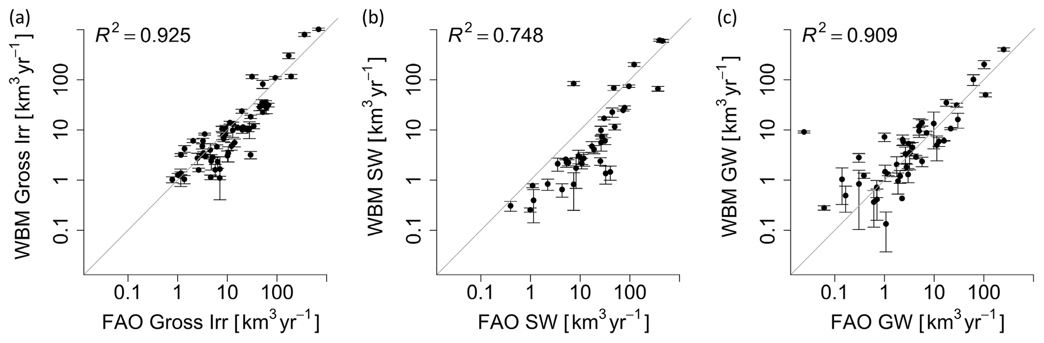
Figure 3Annual irrigation water withdrawals from WBM compare well to FAO AQUASTAT (FAO, 2016) country-level reported (a) total irrigation, (b) surface water use, and (c) groundwater use. Note that both the x and y axes are on a log scale. Total values from updated simulations (WBM v.1.0.0) are reported in Table 6. Figure modified from Grogan et al. (2017).
Irrigation water extractions. The WBM is often used for agricultural applications. It has therefore been well validated against FAO country-level reported irrigation water extraction data, globally in Grogan (2016), Grogan et al. (2017), Wisser et al. (2008), Wisser et al. (2010a) (Fig. 3), and regionally in Zaveri et al. (2016) and Zuidema et al. (2020). Notably, Wisser et al. (2008) quantifies the high uncertainty in irrigation water withdrawals as a function of input climate and crop-map data. Globally, WBM-simulated average total irrigation water extraction for the years 1963–2002 varies from 2200 to 3800 km3 yr−1 in Wisser et al. (2008), with the large difference in values entirely due to the choice of climate input and crop map. While the evaluation data used in all the WBM publications are fully independent of model input data, it should be noted that most irrigation water extraction data are reported statistics, not direct observations.
Additional validation and evaluation metrics. In addition to river discharge and irrigation water extractions, regional studies were evaluated against metrics that are relevant to their application. For example, Zaveri et al. (2016) qualitatively evaluated the WBM's change in groundwater levels in the Indian state of Punjab using data on well levels; Grogan et al. (2020) evaluated simulated SWE across northeastern North America, and Zuidema et al. (2020) evaluated onset timing of the WBM's snowmelt. The evaluation of SWE found that, for most study sites in the northeastern United States, goodness-of-fit (r2) values were >0.5, but model performance was poor where winter precipitation is dominated by lake-effect snow and where climate is moderated by the coastal warming effect (Grogan et al., 2020). Zuidema et al. (2020) found that the timing of peak runoff generation due to snowmelt was well-captured by WBM, but the onset of snowmelt had an early bias in most years.
Validation of FrAMES. The functions of the FrAMES model (Wollheim et al., 2008a, b; Stewart et al., 2013) for river temperature and in-stream nitrogen concentrations have been incorporated into the open source version of the WBM described here. Despite having a different name, FrAMES is part of the WBM family because it added modules for in-stream processes to the WBMplus model code base (see Sect. 5 below). While there is yet to be a published evaluation of the open source WBM implementation of these functions, the nitrogen functionality of the FrAMES model is evaluated globally in Wollheim et al. (2008a) and regionally in Samal et al. (2017) and Stewart et al. (2011). River temperature simulations are evaluated across northeastern North America in Stewart et al. (2013). FrAMES also has an in-stream chloride module; while the WBM does not have this module implemented yet, chloride is an informative metric for evaluating river discharge as this solute is a conservative tracer. We report chloride validation findings of FrAMES here to show how well discharge matches observations since the river discharge functions in WBM and FrAMES are the same. In Zuidema et al. (2018), simulations of river discharge, temperature, and chloride in the Merrimack and Piscataqua River watersheds of New England, United States, were assessed using approximate Bayesian computation (Sadegh and Vrugt, 2013), which provides information on the best regional parameterization for the model. The best parameter estimates resulted in simulated flow-duration curves with an NSE value of 0.93 compared to USGS gage data. Further, Zuidema et al. (2018) found that default WBM parameters for the hydrodynamic groundwater constant and CSRP, while slightly different from the best-performing parameters, still resulted in good agreement with observations.
3.2 Open source WBM model evaluation
We reviewed previously published WBM validations above. As none of the prior versions of the WBM code have been released under an open-source software license, it is important to validate the exact model structure in this first open source release. Previous versions of the WBM and related model code (Table 7) all used the same underlying structure as WBM v.1.0.0 with regards to all the basic terrestrial water balance variables: ET, soil moisture balance, surface runoff generation, subsurface runoff (aka baseflow), shallow groundwater recharge, and river routing. The most recent WBM publications (since 2016) have included the same agricultural water use module as WBM v.1.0.0; tracking as described here, was first implemented in Grogan et al. (2017). Differences between prior publications and WBM v.1.0.0 as described here are mainly in parameter values (here we use all default values for a general model demonstration), and in some cases, recent publications have implemented additional region-specific modules not included in WBM v.1.0.0 (e.g., Zuidema et al., 2020).
In this section, we evaluate results from a global open source WBM simulation that uses publicly available data inputs, and provides a comprehensive selection of tracking outputs. The simulation ran for 270 h on a Dell PowerEdge R510 with Intel Xeon processors (2.93 Gbps) and simulated 2.3 M grid cells for 10 years following 10 years of spinup.
3.2.1 Model setup
Here, we use a global spatial resolution WBM simulation of 5 min for evaluation. The WBM is first initiated with a 10-year spinup to bring stocks to an equilibrium state. Results shown below are from simulated the years 2000–2009. All model input datasets are listed in Table 4. All parameters are set to default values. The model initialization file used for this simulation is available from Grogan et al. (2022).
Table 4Model input datasets for WBM simulations presented here.
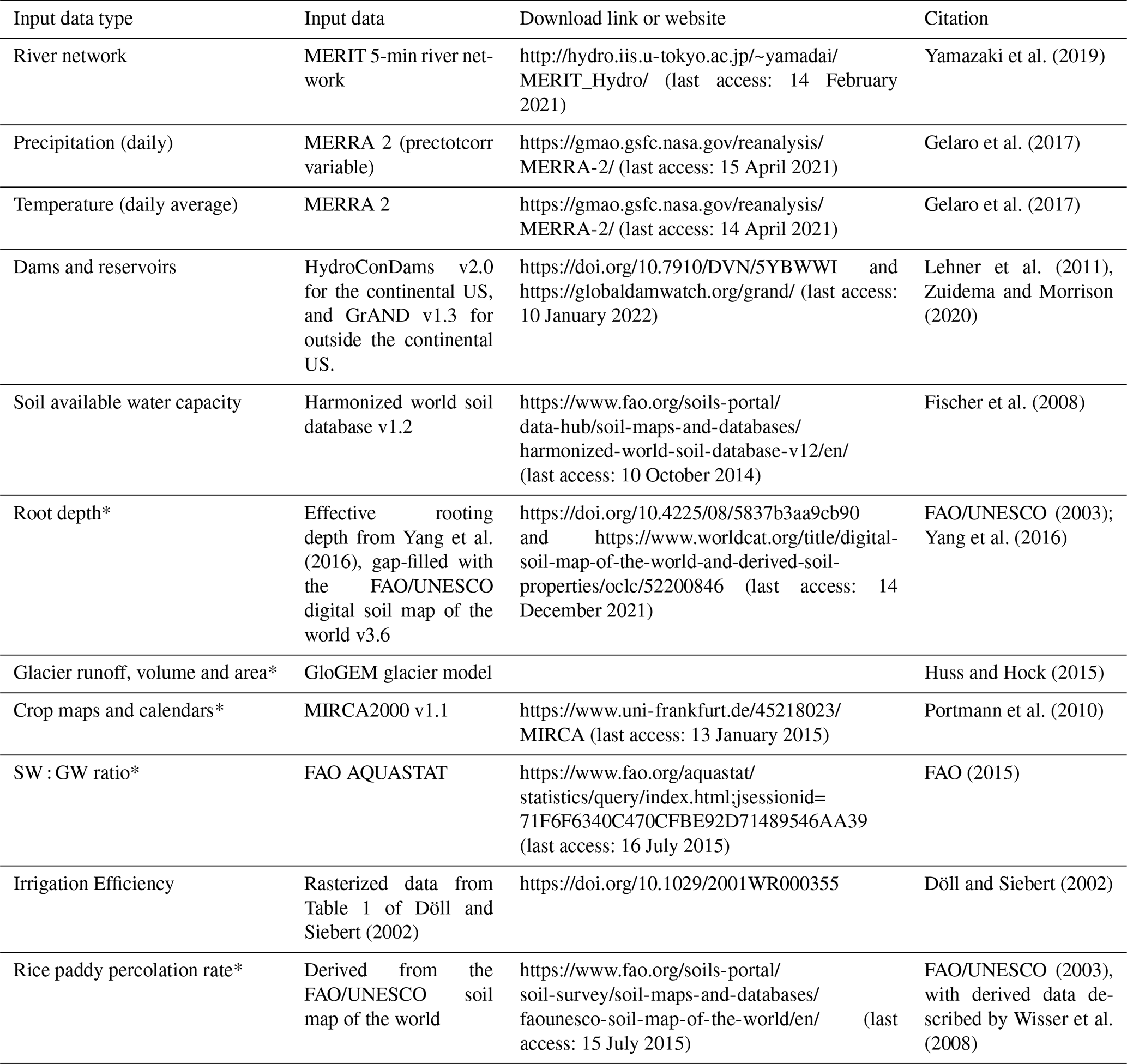
* Primary data were processed for formatting, gap-filling, or to generate a calculated product; the resulting formatted files are provided for download at https://wbm.unh.edu/ (last access: 4 March 2022; Grogan et al., 2022) for simulation reproducibility.
3.2.2 Evaluation data and methods
River discharge. We evaluate the WBM using default parameter values (Table 1) against daily and monthly river discharge records from The Global Runoff Data Centre (2020) which we downloaded in February of 2020. The GRDC's terms of agreement for users prohibit sharing of these data, but the same data can be requested directly from the GRDC. We also compare WBM global annual river discharge results to other published global estimates (Table 5).
Table 5Model estimates of global river discharge, ordered from lowest (based on the low end of a range, for models that report ranges) to highest. Parentheses show the exorheic + endorheic discharge for studies that provide a separation of external and internal basin discharge.
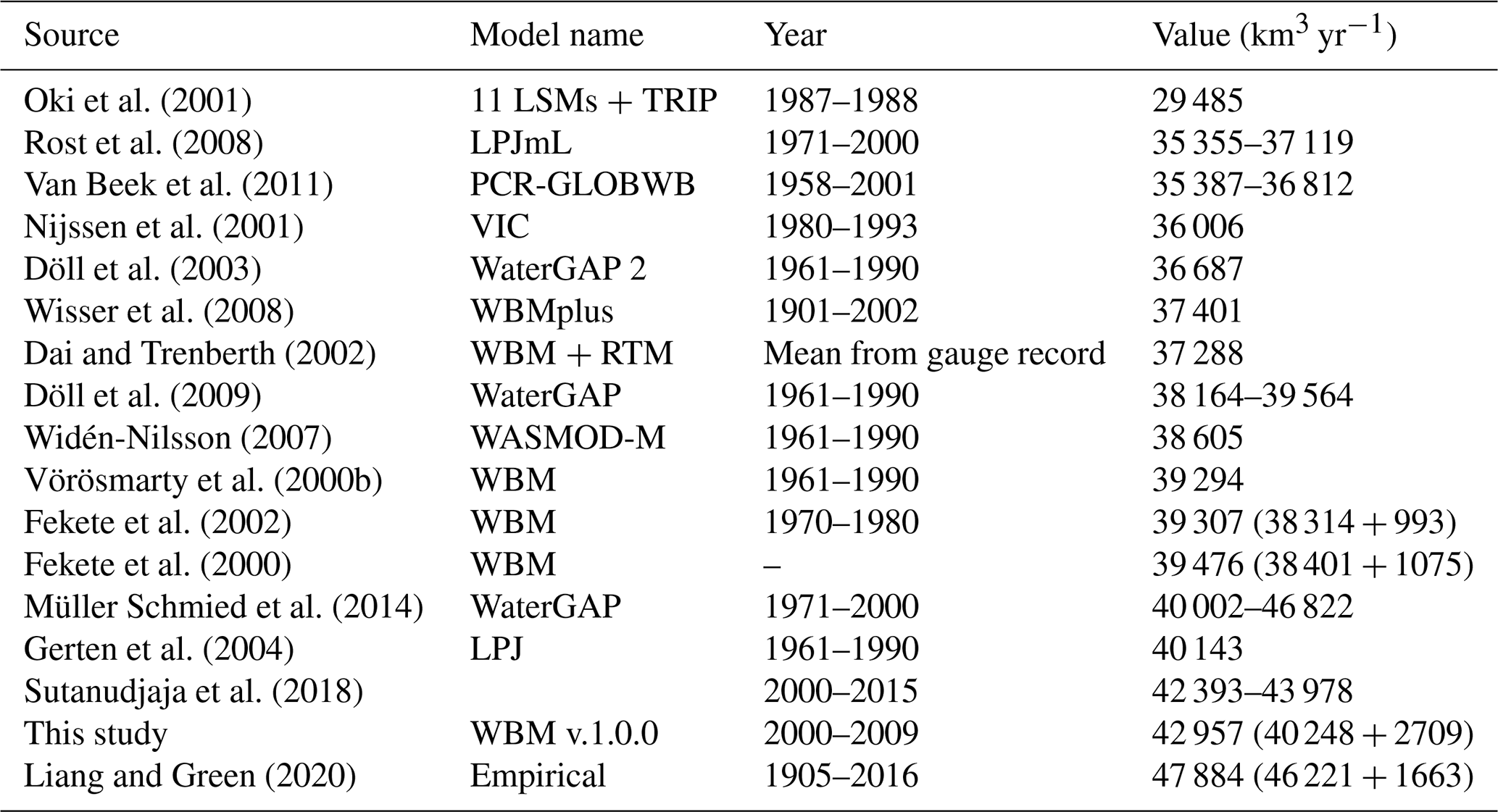
The GRDC stations were filtered based on three criteria: (1) the station must have data within the simulation time frame of years 2000–2009; (2) within the time frame, the station must have at least 12 total observations for monthly evaluation, or at least 365 total observations for daily evaluation; and (3) the GRDC-reported catchment area of a station is compared to the catchment area of the best-matching MERIT river network grid cell within a 3×3 grid centered on the latitude/longitude point defined by the GRDC station. Only GRDC stations with catchment area differences of less than 10 %, once the best area match within the 3×3 grid is identified, are included. Applying these criteria leaves 322 stations for daily and 344 stations for monthly evaluation.
We evaluate simulated daily and monthly average discharge with the index of agreement, d, (Willmott, 1981):
where Pi are predicted (i.e., simulated) discharge values, Oi are observed discharge values, and n is the number of observations. The value of d can range from 0 for a model that is not a better predictor than the mean observed value, to 1.0 for a perfect match of predictions to observations.
In order to measure systemic bias, we also calculate the mean bias error (MBE):
We additionally calculate the NSE (Nash and Sutcliffe, 1970) and Kling–Gupta efficiency (KGE; Gupta et al., 2009) metrics, which are both classic skill scores that indicate whether model skill is better than predicting the mean of the observations (value >0 indicates better skill).
Irrigation water withdrawals. We compare WBM-simulated irrigation water withdrawals by source to reported country-level water withdrawal statistics from AQUASTAT (FAO, 2016), as well as other model-based estimates of withdrawal in the literature.
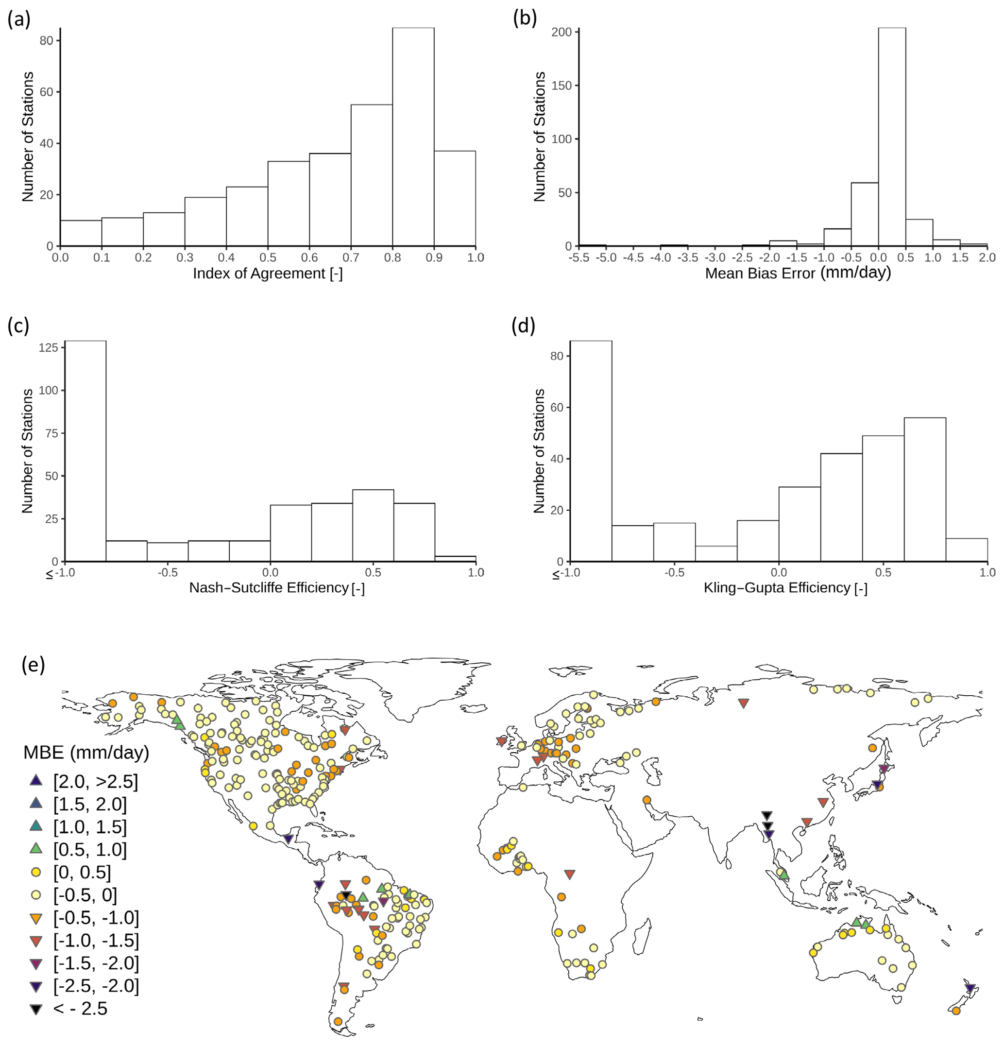
Figure 4Frequency distribution of the index of Agreement (a), the mean bias error (b), the Nash–Sutcliffe efficiency (c), and the Kling–Gupta efficiency (d) for daily average discharge. Panel (e) shows a map of mean bias error in daily discharge [mm d−1], illustrating the spatial variation in bias. The average index of agreement is 0.56, and average mean bias error is −0.07 mm d−1.
3.2.3 Results
Daily river discharge. Overall, global daily average discharge is simulated with moderate agreement to observations; the average index of agreement over all stations is 0.56, and the average MBE is −0.07 mm d−1 (Fig. 4a and e). We find that 43 % and 54 % of basins have values greater than 0 for the NSE (Fig. 4c) and KGE (Fig. 4d) metrics, respectively. However, there is substantial spatial variation in these metrics, with the mean highly influenced by the relatively large number of GRDC stations in the Americas compared to other continents. The lowest single river discharge MBE value is −5.5 mm d−1, which occurs in Southeast Asia (Fig. 4b).
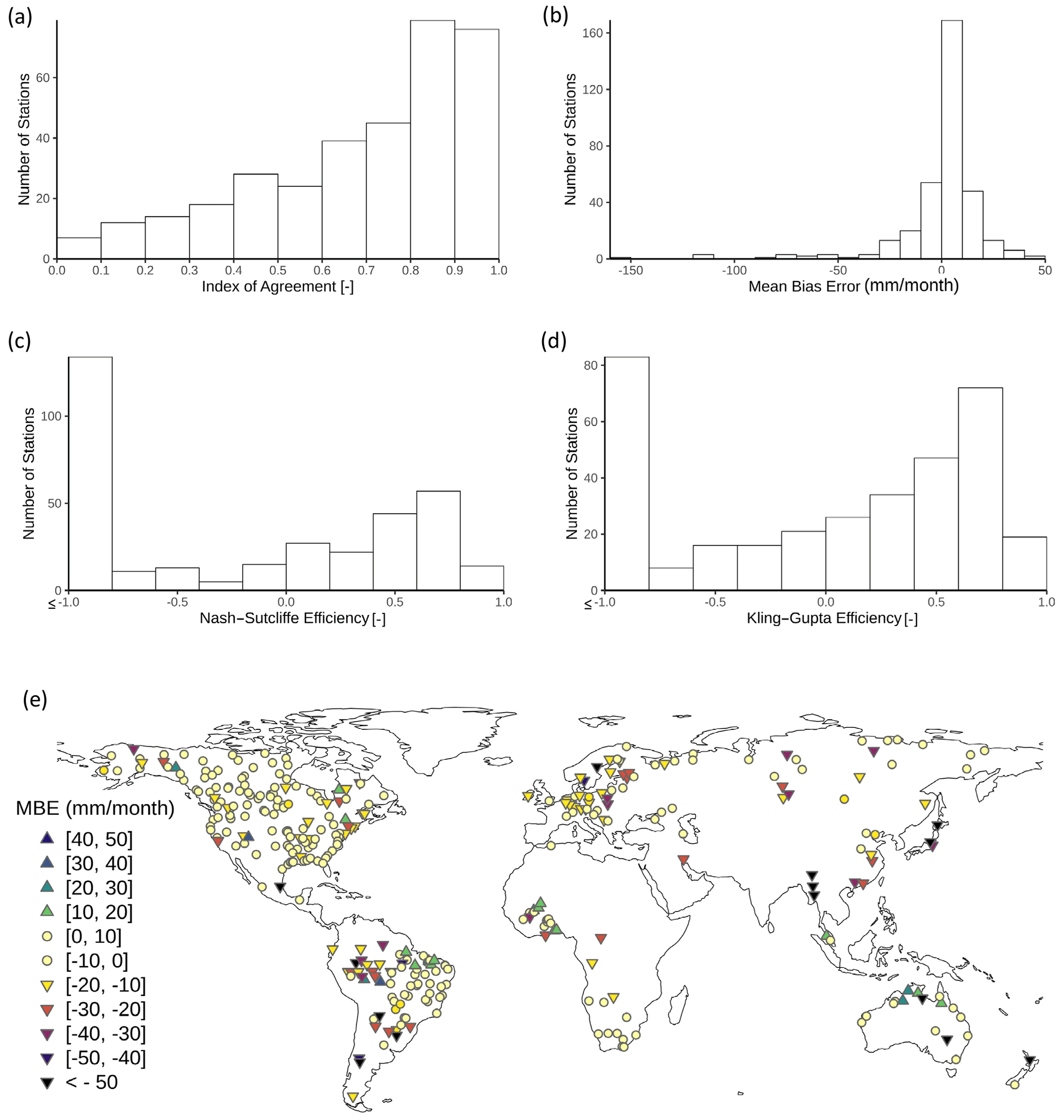
Figure 5Frequency distribution of the index of agreement (a) the mean bias error (b), the Nash–Sutcliffe efficiency (c), and the Kling–Gupta efficiency (d) for monthly average discharge. Panel (e) shows a map of mean bias error in monthly discharge [mm per month], illustrating the spatial variation in bias. The average index of agreement is 0.69, and average mean bias error is −0.14 mm per month.
Monthly river discharge. Overall, global monthly average discharge is simulated with good agreement to observations; the average index of agreement over all stations is 0.69, and the average MBE is −0.14 mm per month (Fig. 5a). We find that 48 % and 58 % of basins have values greater than 0 for the NSE (Fig. 5c) and KGE (Fig. 5d) metrics, respectively. These results are consistent with Wisser et al. (2010a), even though different climate inputs and simulation time series were used.
Despite the global average good agreement, there is significant spatial variability, with lower MBE values across much of South America and East Asia (Figs. 4e and 5e). There are also notably large regions without any evaluation data that meet the criteria for inclusion in this analysis, including South Asia, northern Africa, and the Middle East. Further, MBE values in arid regions will always appear small due to the very low values in river discharge; relative bias metrics are better evaluation tools for these regions.
Annual discharge comparison. Many prior studies have estimated global river discharge (Table 5), providing a range of values from as low as 29 485 km3 yr−1 (Oki et al., 2001) to as high as 47 884 km3 yr−1 (Liang and Greene, 2020). Variation between estimates is caused by several factors, including but not limited to model structure, model calibration, input data, years simulated, simulation domain (e.g., some studies exclude Greenland and/or Antarctica), and inclusion of anthropogenic impacts. See Müller Schmied et al. (2014) for a review and analysis of GHM global discharge sensitivity and calibration. Global annual river discharge as simulated by WBM v.1.0.0 for the years 2000–2009 is 42 957 km3 yr−1, which is within the range of prior studies (Table 5). Fewer studies report the contribution of exorheic (basins that discharge to the ocean) and endorheic (basins that discharge to internal seas) discharge. The WBM v.1.0.0 estimates that exorheic discharge is 40 248 km3 yr−1, and endorheic discharge is 2709 km3 yr−1. The exorheic estimate falls within published values, which range from 38 314–46 221 km3 yr−1. The WBM v.1.0.0 estimates higher endorheic basin river discharge than previous studies which report estimates of 993–1603 km3 yr−1. It is possible that this higher estimate reflects WBM v.1.0.0's inclusion of Greenland, along with inclusion of runoff from glaciers, which is not present in most previous studies.

Figure 6WBM-simulated irrigation water withdrawals compared to FAO AQUASTAT-reported values, by country. The 1:1 line is shown in gray. Countries with FAO-reported agricultural water withdrawals <100 km3 yr−1 are shown in the inset. Countries with FAO-reported agricultural water withdrawals >50 km3 yr−1 are labeled.
Table 6Global estimates of total irrigation water withdrawal, including this study's simulation.
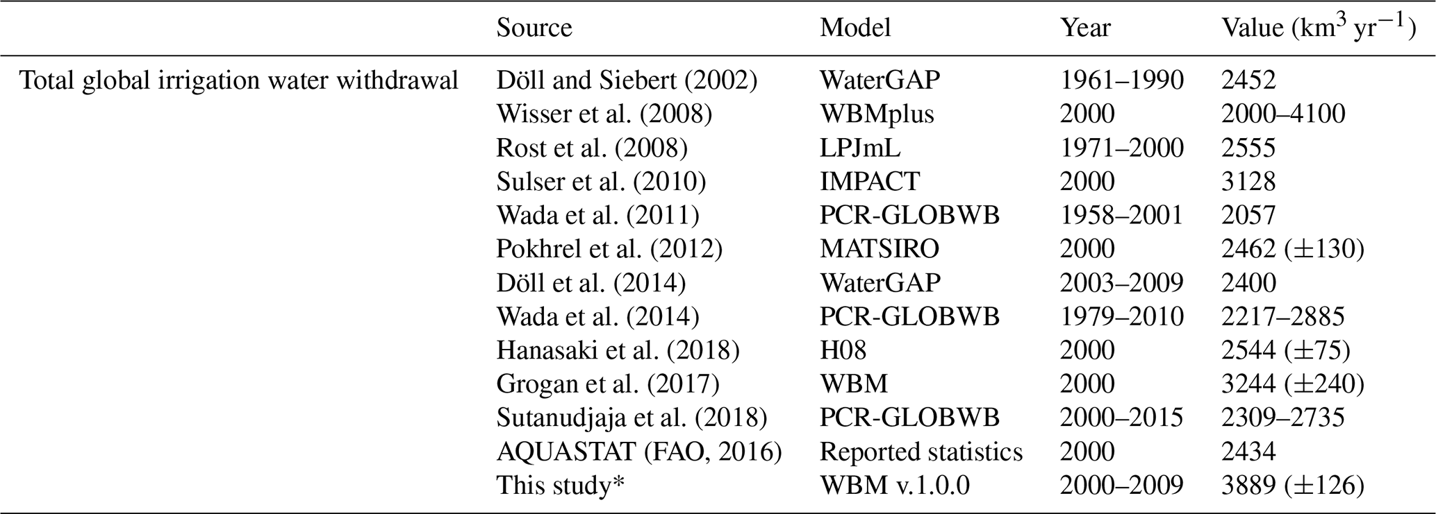
* Uncertainty estimate is the standard deviation of annual values from 2000–2009.
Irrigation water withdrawals. Simulated irrigation water withdrawals fall on the high end of previously reported GHM-simulated global irrigation water use (Table 6). Note that Wisser et al. (2008) demonstrated a large uncertainty in GHM-simulated global irrigation water withdrawals as a function of input climate and crop-map data. The WBM simulations match well to AQUASTAT (FAO, 2016) country-level statistics on agricultural water use (Fig. 6) for most countries, with an R2 value of 0.84 on a linear regression of country–year combinations included in both the AQUASTAT database and WBM simulations. However, the WBM simulates 2 to 3 times higher irrigation water use in China and Pakistan than reported by AQUASTAT, accounting for most (up to 90 %) of the difference between the WBM and the mean of other GHM-simulated global agricultural water withdrawals (Table 6). As can be seen in Figs. 4 and 5, river discharge across much of Asia is underestimated by this WBM simulation, which may reflect a low bias in precipitation inputs thereby contributing to the overestimation of irrigation water withdrawals in China and across much of Asia (Fig. 6). Data from Grogan (2016) show that irrigation water requirements can be highly sensitive to climate inputs, especially in Asia; comparing six different climate inputs to WBM, results for irrigation water requirements in China vary from 615 km3 yr−1 (driven by the NCEP (Saha et al., 2014) climate data) to 1276 km3 yr−1 (driven by the UDEL (Willmott and Matsuura, 2001) climate data).
The WBM's unique water source tracking functions distinguish it from other GHMs. Here, we demonstrate the suite of tracking options available to model users: primary source tracking (Sect. 4.1), return flow tracking (Sect. 4.2), and land surface label tracking (Sect. 4.3). Tracking output explains how the model arrives at simulated water stocks and flows. For example, river discharge is a collection of water flowing from different sources. These tracking functions make explicit what the sources are within the model that form the simulated discharge. We caution that any model can arrive at a well-validated result through erroneous assumptions and aggregate errors. We find that the component tracking increases the transparency of model assumptions; however, evaluation data for these tracking functions are not available at this time, and we rely on evaluation of the stocks and fluxes themselves (not the component composition) for model evaluation. Future regional scale work could make use of emerging datasets on DNA or geochemistry such as chloride (Zuidema et al., 2018) to evaluate return flows from human and agricultural uses (Plummer et al., 2000), and stable water isotopic methods may be able to distinguish rain, snowmelt, and glacier water sources (Fekete et al., 2006; Fan et al., 2016; St Amour et al., 2005).
Here, we use the same global, 5-min spatial resolution WBM simulation as used for model evaluation to demonstrate the first two tracking examples: primary source tracking and the return flow tracking, as multiple tracking functions can be implemented within a single model run.
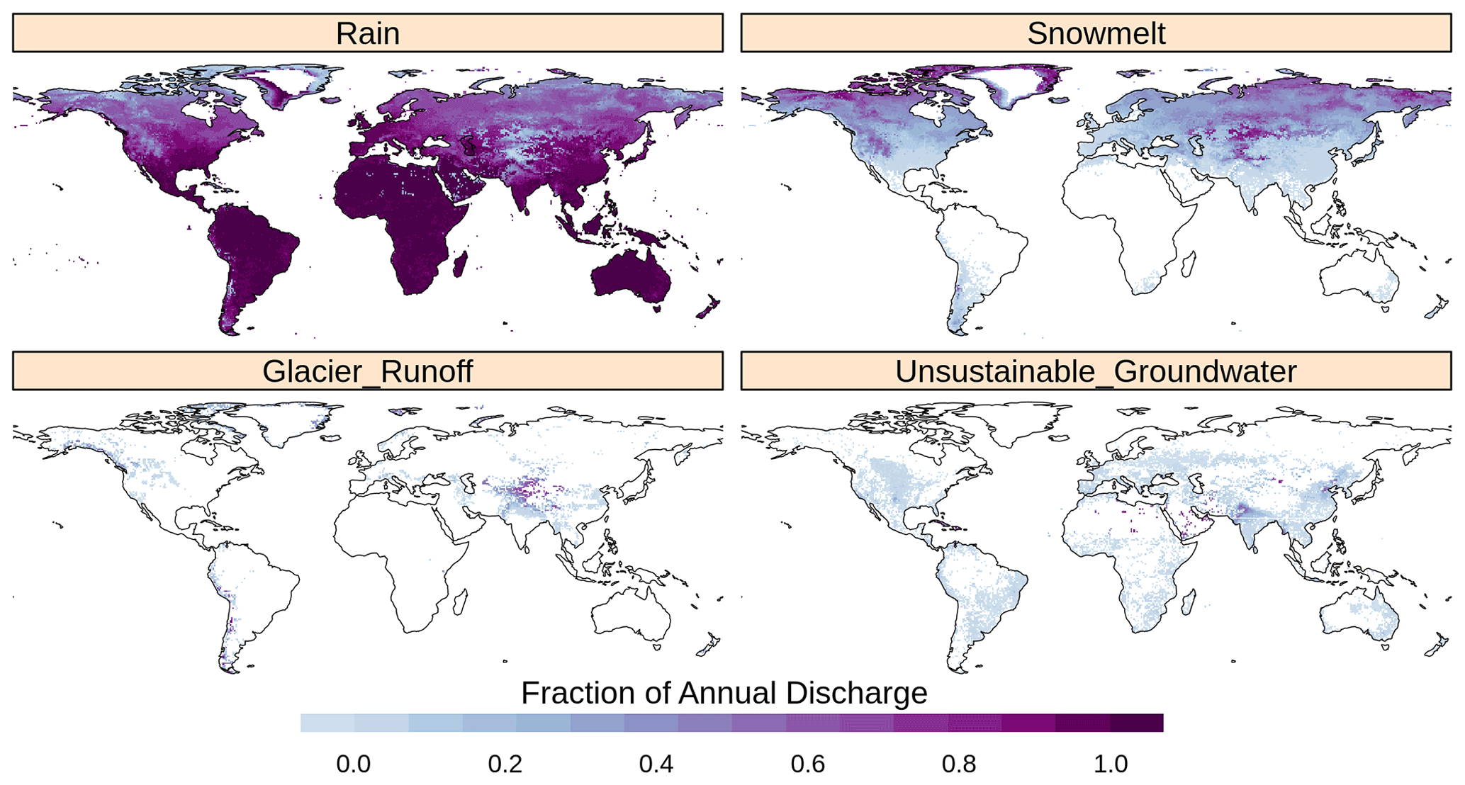
Figure 7The fraction of average annual discharge composed of the four different primary source water components used in the primary source tracking method.
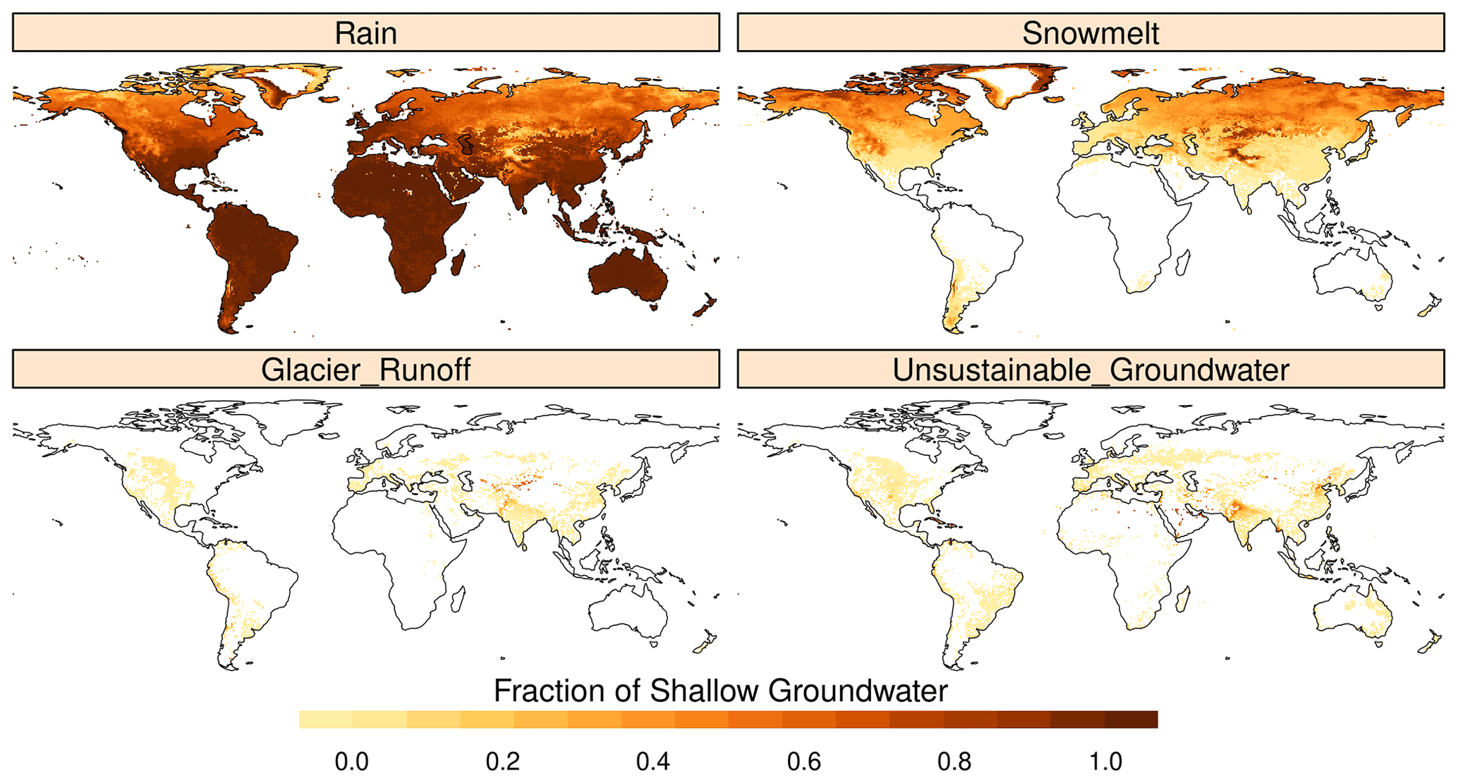
Figure 8The fraction of average annual shallow groundwater storage composed of the four different primary source water components used in the primary source tracking method.
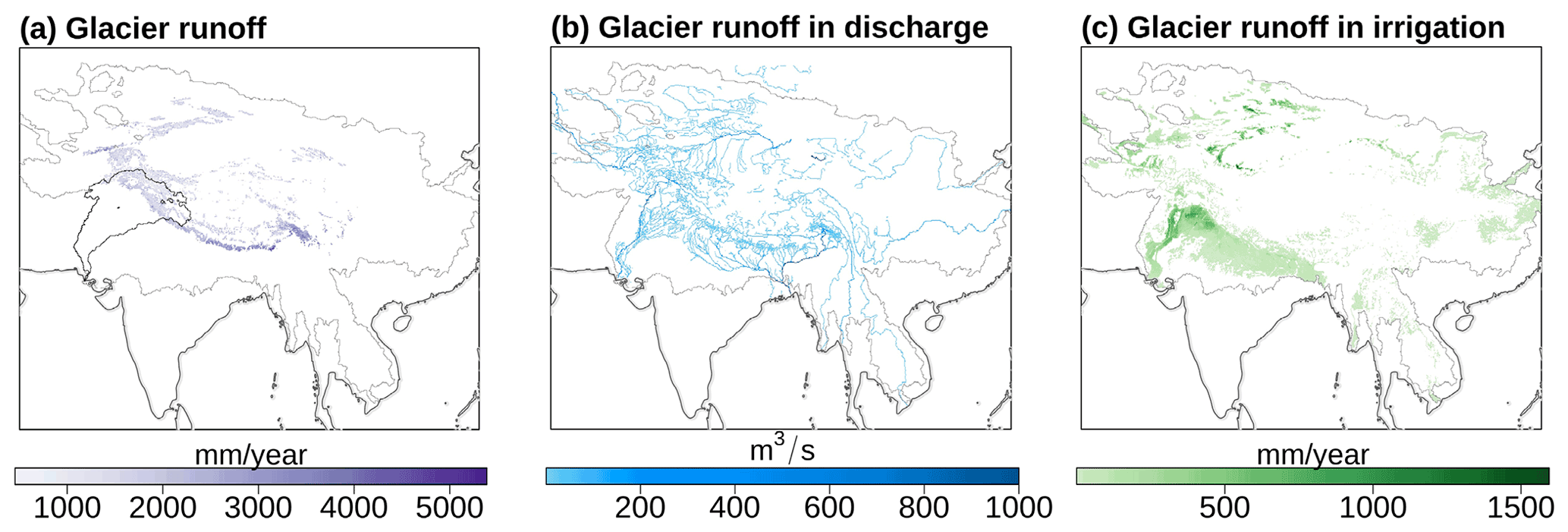
Figure 9Tracking glacier runoff (a) downstream through rivers (b) and irrigation water use (c) in High Mountain Asia, a region where glacier meltwater is an important resource. While glacier water originates in the mountains, its use in agriculture is extensive due to re-use through the river network and shallow groundwater stores, and retention in and distribution from large reservoirs. The boundary of all High Mountain Asia basins with glaciers at their headwaters is shown in gray. Panel (a) also shows the Indus River basin boundaries for reference to compare with Fig. 10.
4.1 Primary source tracking
The primary source tracking function identifies all water entering the model system as originating from one of four categories: rain, snow, glacier runoff, or unsustainable groundwater. Note that the shallow groundwater pool is filled with water from one of these categories, hence shallow groundwater and baseflow are not primary source categories. Glacier runoff, as taken from a glacier melt model such as GloGEM (Huss and Hock, 2015) or the more recent PyGEM (Rounce et al., 2020a), includes all the water fluxes that occur on the glaciated area. This means that glacier runoff includes the rain, snowmelt, and glacier ice melt from the glacier area. Figures 8 and 9 show the fraction of average annual discharge (Fig. 7) and shallow groundwater (Fig. 8), composed of each of the primary sources, for each grid cell. Global discharge is dominated by rain over most of the globe, with snowmelt being an important contributor at high latitudes and high altitudes, and both glacier runoff and unsustainable groundwater important regionally. The composition of shallow groundwater mirrors that of discharge. Due to human redistribution, water inputs into the land surface can support streamflow and agriculture far from where they occurred, as can be seen in Fig. 9, which shows the source, distribution, and use of glacier runoff. As can be seen in Fig. 10, water sources like glacier runoff and unsustainable groundwater contribute to river flows, and therefore water resources, far downstream from where glacier runoff or pumped unsustainable groundwater is input into the river network. Figure 10 also shows how tracking can identify different contributions of source water to river flows through the year, as well as how glacier runoff is an important component of water supply far downstream in the basin late in the year.
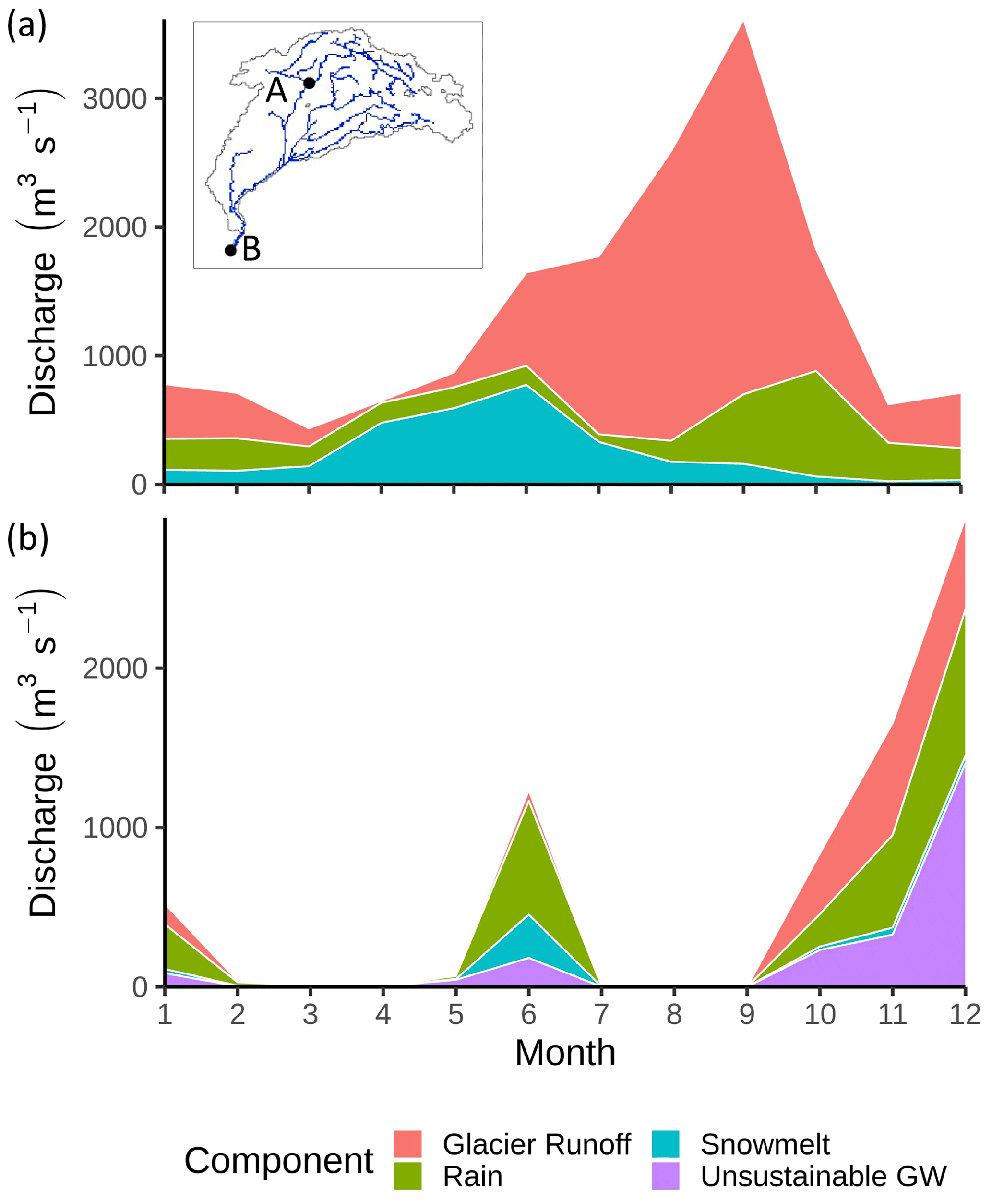
Figure 10Monthly discharge by primary source component at two points (A shown in panel a, B shown in panel b) along the Indus River (basin shown in inset). Point A is in the headwaters, with substantial contributions from snowmelt and glacier runoff. Point B is the river mouth. The mouth of the Indus River runs dry in this simulation due to both the seasonality of precipitation in the monsoonal region, and the large amounts of water extracted from the river for use. This use and re-use of water can be seen in the distribution of primary water sources remaining at the mouth of the river, which include unsustainable groundwater (purple) that was pumped from upstream sources, as well as snowmelt (blue) and glacier runoff (red), both of which are generated far upstream of the river mouth.
4.2 Return flow tracking
The return flow tracking function labels water that flows back to the system after being extracted for irrigation, livestock watering, domestic, or industrial use. Irrigation return flows are identified separately from water returned by other human uses; however, returns from domestic, industrial, and livestock uses are not tracked individually (but rather lumped into one return category) for parsimony. These return flows have water quality implications, and through this tracking function, the WBM can identify when a body of water is increasingly composed of water returned from anthropogenic activities. At the beginning of a simulation, all water is considered relict, which assumes no knowledge of the source of the water. New water entering the system during the simulation period as precipitation or glacier runoff is tagged as pristine water. This functionality was first published in Zuidema et al. (2020).
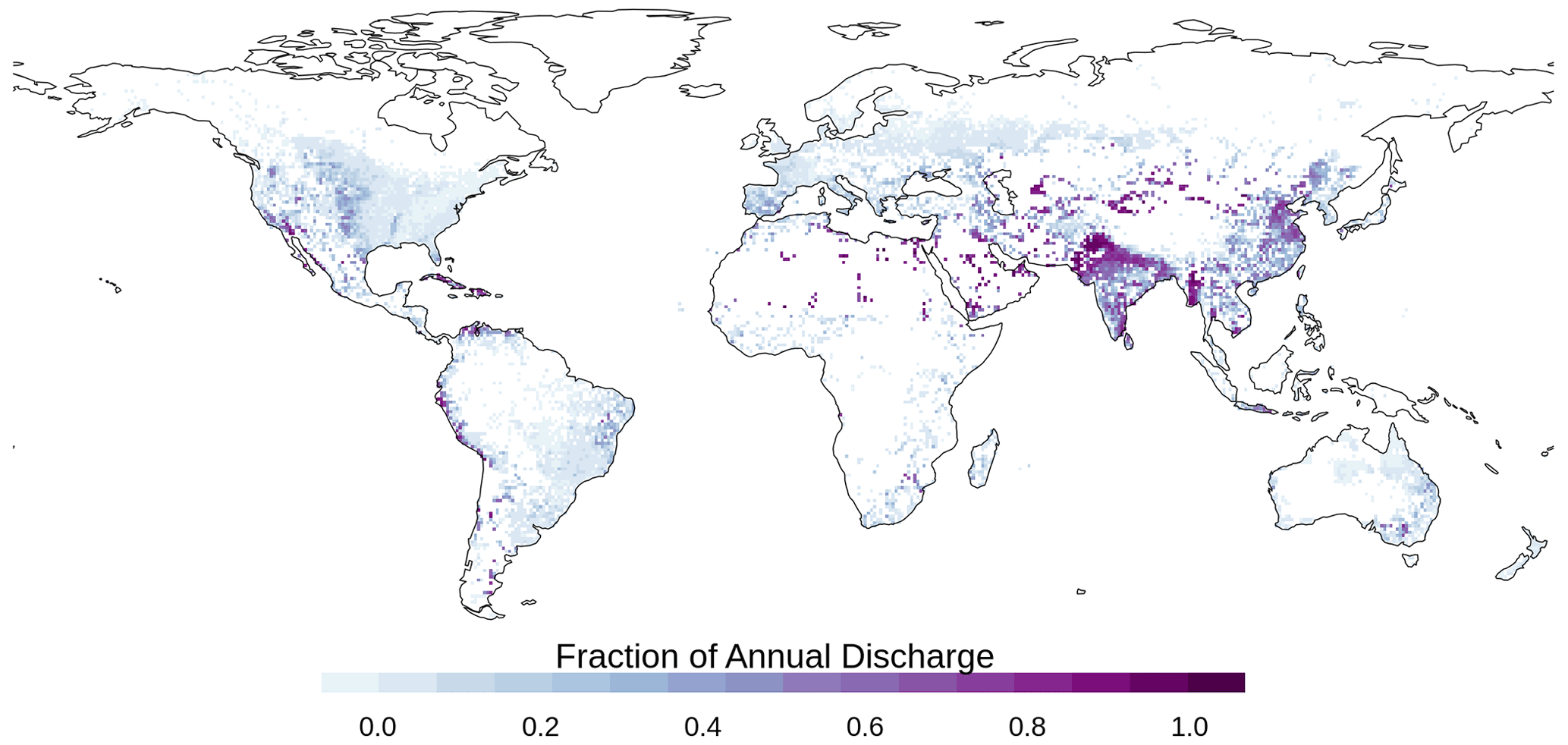
Figure 11Fraction of average annual discharge composed of irrigation return flow water, simulated by the return flow tracking function. The large fraction of irrigation return flows in northern India and Pakistan results from this region being one of the most intensively irrigated regions in the world, combined with very low (∼30 %) classical irrigation efficiency (Zaveri et al., 2016; Grogan et al., 2017). This combination means that large volumes of water are extracted for irrigation, and nearly two-thirds of that water returns to the system.
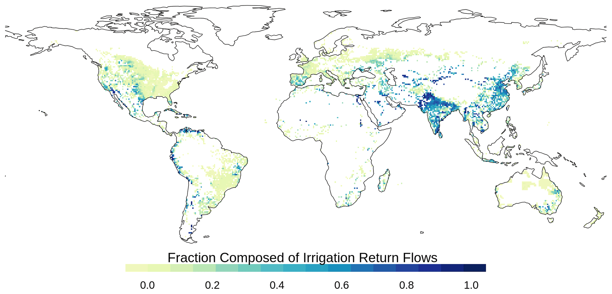
Figure 12Fraction of average annual irrigation withdrawals composed of prior irrigation returns simulated by the return flow tracking function.
Figure 11 shows the fraction of average annual discharge composed of irrigation return flows, and Fig. 12 shows the fraction of irrigation water withdrawals composed of irrigation return flows (water re-use). These fractional values cannot exceed 1, even as return flows are re-used multiple times; when return flow water is extracted again for re-use, it simply retains its identity as return flow, and does not contain any new information about the number of times it has been extracted. Return flows from all human water uses contribute to water quality issues, including excess nutrients from irrigation returns and pathogens from domestic and livestock returns, some proportion of which may be attenuated by the river network depending on flow conditions (Huang et al., 2022) before being used again. Further, re-use of return water is an important consideration in studies evaluating the “efficiency” of irrigation or other abstractions. Management actions that decrease returns in one region may reduce water availability downstream, which may promote extraction of alternative and potentially less sustainable sources of water (Grafton et al., 2018; Grogan et al., 2017).
4.3 Land surface attribute tracking
4.3.1 Model setup
Here, we use the same set of model inputs and parameters as the global 5-min spatial resolution WBM simulation described above, but reduce the spatial domain to only simulate grid cells downstream of headwaters in the state of Wyoming, United States. One additional model input is required for the land surface attribute tracking: identification of which grid cells are within each of the US states that intersect the spatial domain. This input (which includes a gridded file and an accompanying attribute text file) allows the WBM to track water that originates as runoff within each US state as it travels downstream through four major river basins (the Mississippi, Columbia, Colorado, and the Great Basin) which span both sides of the continental divide. Applications of this technique would be useful for research involving transboundary conditions in river basins or using land-cover masks to understand urban/rural or forest/non-forest effects in regional hydrology.
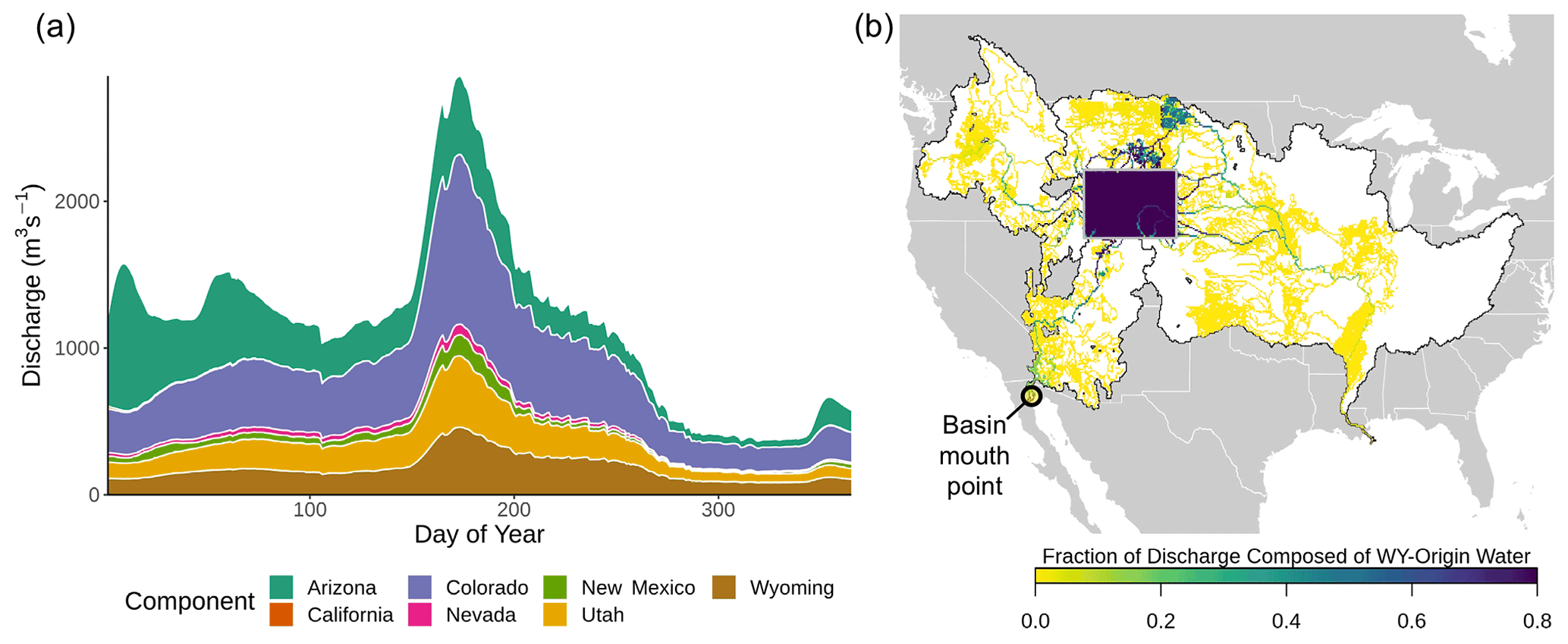
Figure 13Demonstration of the WBM's land surface attribute tracking function. (a) Discharge at the mouth of the Colorado River basin (basin mouth point shown in panel (b). Colors show contribution of water from seven different US states, accounting for the movement, storage, and cycles of extraction occurring across the basin's many upstream water uses. (b) Fraction of Wyoming (WY) waters in river discharge on 1 July 2009. Basins in the study domain are outlined in black; gray regions are not simulated; the state of WY is outlined in light gray. The state of WY appears dark in (b) because nearly all river discharge within the state of WY is >80 % WY-origin water. Where rivers enter WY, such as the North Platte River, the color lightens as a larger portion of non-WY water enters the state boundaries; as more WY-sourced water is added to those rivers, the color becomes progressively darker.
4.3.2 Results
Tracking runoff generated by different US states demonstrates how the land surface attribute tracking can be used to identify contributions of water from any user-identified spatial attributes. The basins simulated here all contain cities and both extensive and intensive irrigated areas; the land surface attribute tracking maintains the US state identification of all surface and shallow groundwater withdrawals and return flows as water travels through the system from headwaters to river outlets. Figure 13a illustrates how this tracking is useful for identifying multiple land attribute contributors to river discharge at a point. Figure 13b demonstrates the spatial distribution of water from one land attribute through many downstream systems. Particularly in Fig. 13b, we can see how human extractions of water – which can occur across grid cells – spreads the tracked land attribute's contributed water across the landscape.
Table 7Major WBM code branches, along with their history of new functionality and whether the code branch is still in use.
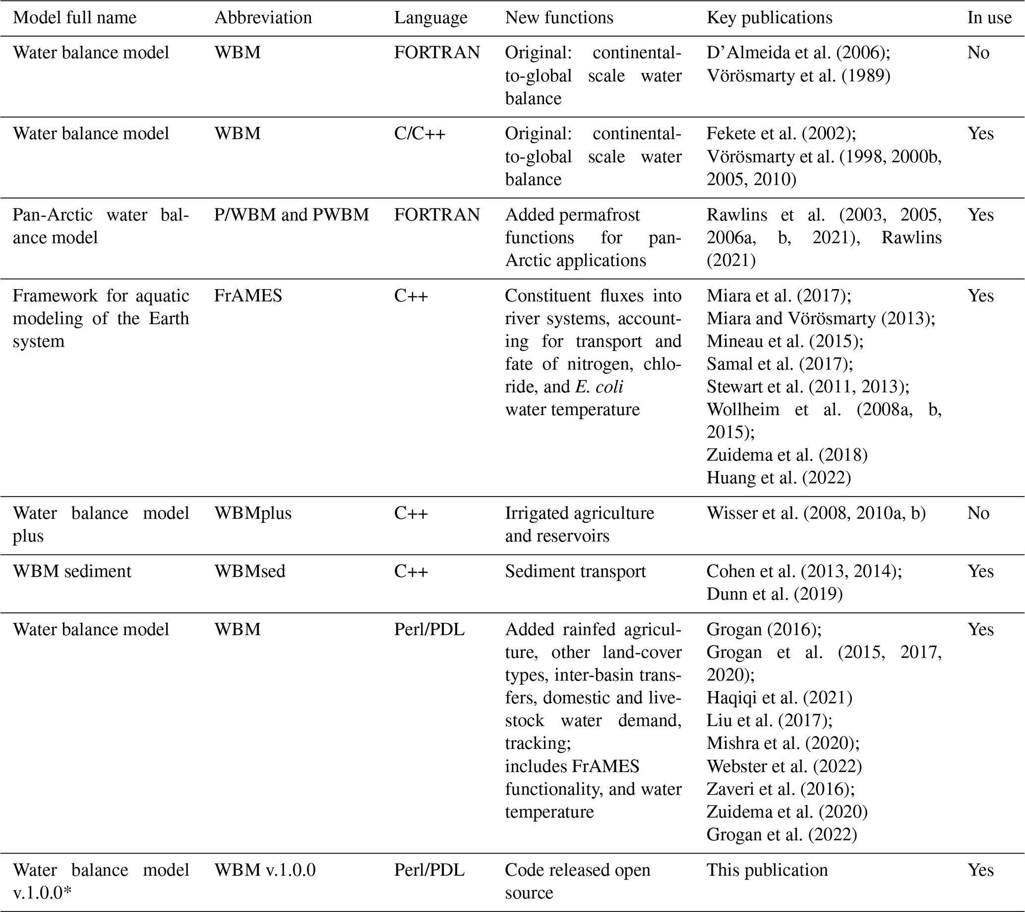
* This version of WBM is the open source model described in this paper.
Brief history of model code development. The WBM was originally written in FORTRAN, and first published in Vörösmarty et al. (1989). The first publication described the WBM as a continental-scale model of water balance and fluvial transport, and presented an application to South America. The first global applications were published in Vörösmarty et al. (1998, 2000a). Throughout its 30+ year history of development, the WBM has been re-written in several programming languages, and branches have been developed for specific applications (Table 7). Table 7 describes each branch of the WBM, with its abbreviation (e.g., WBM vs. PWBM), the application for which the branch was developed, and key publications. Many of the branches are still in use by a variety of research groups, including researchers at the University of New Hampshire (WBM v.1.0.0), City College of New York (WBM), University of Alabama (WBMsed), and University of Massachusetts (PWBM).
WBM Open Source code. The WBM version described here is written in Perl/PDL. The coding language was changed from C++ to Perl/PDL by the University of New Hampshire research group in 2010 to make use of the following PDL functionality that was unique to that language at the time:
-
efficient parallel processing of matrix operations on large spatial matrices allowing increased computational performance similar to C or Fortran through the use of binary PDL operators/functions and multithreading;
-
adding pre-compiled custom functions written in inline C (PDL PP modules); and
-
fully integrating the river transport module with the land surface component of the WBM to simulate the full downstream effects of water withdrawals from the rivers. Prior versions of the WBM resolved the time component prior to the spatial component of the model; this prevented implementation of water extractions and inter-basin transfers.
The open source Perl/PDL version of the WBM described here includes all the functionality of the original FORTRAN WBM model, the WBMplus model, and some aspects of the FrAMES model. All model branches run on Linux operating systems. The open source WBM code described here is composed of three main files: (1) wbm.pl, which is the main model script; (2) WBM.pm, a module providing WBM-specific functionality; and (3) RIMS.pm, a module providing geospatial and temporal transformation utilities. The entire modeling framework is dependent on other software: Perl, PDL, GDAL, ogr, and NetCDF. The model input data repository (https://wbm.unh.edu/, last access: 4 March 2022, Grogan et al., 2022) also includes a singularity container which has pre-installed the required operating system and software dependencies for ease of model use by the research community.
The WBM can run high-density grids in a simulation domain up to about 3 million active grid cells on an average rack system server and utilize CPU parallelization (multi-threading) for a performance boost. Smaller spatial domains can be run on a personal desktop or laptop computer.
Code implementation. WBM is rasterized and generally used with uniformly spaced gridded data (typically in geographic coordinates, but accepting any GDAL-readable format), keeping values of grid-cell area in memory for flux calculations. The model is modular, with many options to turn irrigation and other human water extractions on or off. Options are controlled by the user through a selection of direct inputs, on/off flags, and output variables requested of the model. Stocks and fluxes including irrigation demand, ET, and runoff generation are calculated in the first portion of the time-step loop utilizing vectorized and efficient array utilities of PDL. Water entering stream reaches throughout the network is then submitted to a routing function that traverses a directed, noncyclical graph of all grid cells that ensures an upstream-to-downstream calculation order, written in an inline, pre-compiled format to maximize computational efficiency. In a number of areas, the model makes use of split-operator solutions to facilitate both tracking functionality and the complex interactions between human water withdrawals and natural systems. This simple method allows the WBM to recalculate water stocks and fluxes after water extraction occurs and again after return flows, such that the final stock and flux values at the end of a time step are modified from the first instance of calculation at the beginning of the time step. As noted by others, leveraging of split-operator solutions for hydrologic models provides a tradeoff between efficiency and accuracy in numerical solutions, which is warranted in some cases (Clark et al., 2015).
How to use WBM. The WBM workflow involves 5 basic steps:
-
Prepare input data, metadata, and parameter files;
-
Write a model setup file with the extension “*.init”;
-
Test setup file by running the WBM with flags “-test”, “-noRun”, and “-err”;
-
Execute the model code (wbm.pl);
-
Perform post-processing, if needed, with automatically generated utilities for temporal aggregation of select or all output variables.
A detailed instruction manual is included in the model's Github repository, along with Perl utilities commonly used in Steps 1 and 5.
In Step 1, the model user must collect all input data required for the given model simulation. Each spatial dataset and database must be described in a metadata file with the extension “.init”. All data and model input “.init” files are simple text files with formatting that conforms to a Perl hash. Input file unit conversions (e.g., converting temperature data from ∘C to ∘F) do not need to be performed prior to running the WBM. Instead, the user can define a conversion slope and intercept for linear transformations within the metadata “.init” files, and the WBM will automatically calculate the new units through the RIMS.pm module.
In Step 2, the model user writes a model setup file with the extension “.init” that lists all model inputs as well as other key parameters such as the start year, end year, list of output variables to save, and output directory location. This setup file points directly to the input data “.init” metadata files, and includes options to directly define parameter values and set binary on/off flags for particular modules. Most important is the identification of the digital river network. The input river network file determines the model simulation grid spatial resolution, spatial extent, projection, and defines non-land grid cells (which are set to a no-data value). Other input datasets will automatically be clipped (extent reduced) and re-gridded (either through resampling or aggregation) to match the extent and grid-cell resolution of the input river network file. This means that the model user does not need to do these spatial transformations prior to starting the model.
In Step 3, the user tests the model setup and produces an optional input data pre-processing script. Test mode and “noRun” mode call the input data reading functions from RIMS.pm and set up the model run's output directory. This step is used to identify any errors in the model setup; these are commonly issues such as incorrect file paths, syntax errors in the “.init” files, or formatting errors in the raw data files. Executing wbm.pl in test and noRun mode also automatically generates a custom build_spool.pl script (written to the model run's output directory) that can optionally be executed prior to Step 4 to pre-process all input data files that require requisite spatial clipping, re-gridding, or unit conversions. If build_spool.pl is executed, the results of input data pre-processing are saved as binary files that are read directly by the WBM; these files can also optionally be saved as netCDF files for ease of analysis, so the user can evaluate the results of the processing step. If the custom build_spool.pl script is not executed prior to starting the model in Step 4, pre-processing will automatically be executed in the model's run time. Note that this automatic option only produces binary files and does not output any netCDF files. The build_spool.pl utility can leverage multiple CPUs to efficiently build binary input files; the automatic option processes all binary files in a single process with a steep reduction in model simulation time.
In Step 4, the model user executes wbm.pl via direct command line entry. The code wbm.pl has several flag options, including -h for help, -v for verbose mode, and others described in the instruction manual. The model setup file is the only required argument to wbm.pl. Under the verbose mode, detailed statistics of model run time, domain aggregate water balances, and water supply metrics are reported to the user during each time step, with more complete accounting of water balances reported at the end of each year of the simulation. Model-run state files are written at the end of spinup, and at the end of each year, and (optionally) more frequently. This frequent saving of state files enables users to restart simulations in the event of an interruption (e.g., from power loss) without losing significant wall time. Model output files are written in the same spatial resolution and domain as the input digital river network.
Step 5 is the most application- and user-specific step. The raw daily model output is rarely the final product of analysis; temporal and spatial aggregation or point-location time series extraction are most commonly required to evaluate output and produce research results. The model automatically generates daily-to-monthly and daily-to-yearly temporal aggregations, and the setup file has a binary on/off option that enables automatic temporal aggregation to climatology (daily, monthly and yearly) averages using either the entire simulation period or specified year groups for averaging; there is also an input field for automatic spatial aggregation. The Perl utilities for these operations are included in the model Github repository.
The WBM's simulation of global hydrologic fluxes are similar to many other GHMs (Tables 5 and 6). Global estimates of discharge are in line with other GHM estimates, and correspondence with observations is globally reasonable and error-prone in specific locations. Model performance (Figs. 4 and 5) is best in North America, where observational data density is high, climate reanalysis data used as input data to the WBM have greater observational density to draw from (Gelaro et al., 2017), and the majority of historic regional calibration activities were focused (Stewart et al., 2011; Samal et al., 2017; Zuidema et al., 2018, 2020; Grogan et al., 2020). Low biases in discharge throughout Asia may reflect biases in input precipitation fields (Grogan, 2016), or that globally assumed parameters are unrepresentative of these landscapes. Estimates of discharge predicted by the WBM that are higher than several prior estimates (Table 5) likely reflect a combination of an increased rate of precipitation during recent decades (Blunden and Arndt, 2020), and more advanced estimates of global precipitation (Gelaro et al., 2017). The distribution of model performance metrics presented here (Figs. 5 and 6) are comparable to other recent global syntheses (Lin et al., 2019; Harrigan et al., 2020). While the default parameterization can miss key distinguishing features of local hydrologic responses, the inclusion of anthropogenic processes is a critical feature for providing sufficient hydrologic simulations (Zaherpour et al., 2018). Irrigation withdrawals predicted by WBM v.1.0.0 reflect country-specific estimates from AQUASTAT over most of the globe (Fig. 6). High biases for irrigation water withdrawals in Asia, particularly China and Pakistan, correspond spatially with low biases in discharge and may reflect both data and parameterization issues that should be resolved in work focusing on these specific regions. Considering the high degree of flexibility in WBM parameters and the broad range of modern meteorological input data, reasonable hydrologic simulations should be attainable within any region of the globe. However, it is important for model users to use a spatial resolution appropriate for regional study domains, and to use local data to parameterize and evaluate the model for each new study domain.
The tracking functionality of the WBM opens unique options for model-based experimentation with potentially important management implications within a GHM. Oftentimes, hydrologic modeling studies provide insight into the relative importance or effect of a particular hydrologic process by switching processes on and off, thereby creating slightly different systems. These studies identify the role of a specific process in a system by comparing two or more structural or parametric model configurations with and without representation of a particular process. Such analogies are most powerful when used to understand the effect of hydrologic fluxes which are expected to fundamentally change, such as glacial melt (Rounce et al., 2020a), or have been historically absent in previous hydrologic modeling such as surface depressions (Rajib et al., 2020). Similar approaches may test the effectiveness of different management strategies, such as the effect of managed aquifer recharge on aquifer head and river flow (Niswonger et al., 2017; Tran et al., 2019; Van Kirk et al., 2020; Zuidema et al., 2020). In other cases, this approach has been used to assess the difference between a hypothetical natural system (with no human impacts) and a human-impacted system (Wada et al., 2016).
By using the tracking methods described here, it is possible to attribute a portion of water flows to a specific process, location, water source, or flow path, without altering the represented system from an existing or experimental configuration. This is fundamentally different from the on/off method of evaluating process or source importance that has been more commonly used in the literature. WBM’s tracking module achieves this by attributing a composition of sources or prior influential processes to the water stored and moving within each grid cell. For example, this tracking function facilitates the calculation of irrigation returns in future withdrawals that make the estimation of effective irrigation efficiency (Haie and Keller, 2008) possible under suites of hypothetical management configurations (Zuidema et al., 2020). As there are no equivalent empirical analogues, evaluating the tracking component compositions of any flux is not presently possible; however, tracking functionality creates a more transparent representation of the assumptions that drive model results.
As described in Weiler et al. (2018), several different water tracking methods have been employed by regional hydrologic models, though as of the time of this writing, no GHM other than the WBM employs these types of tracking methods. Tracking methods of regional hydrologic models include synthetic scalar transport, solute transport, particle tracking, and the “effective tracking” used in HBV-Light (Stahl et al., 2017; Weiler et al., 2018). The WBM's tracking fits into the class of effective tracking methods described by Weiler et al. (2018), and is a simplified version of the synthetic scalar transport method, analogous to solute transport where mixing within compartments of the model is substituted for a full calculation of the advection-dispersion equation. Insights provided by effective tracking into the sources of discharge and water provisioning are most relevant for evaluating human water resources (Weiler et al., 2018).
The open source GHM, WBM v.1.0.0, represents not only the natural terrestrial hydrologic system, but also human interactions with water resources. These interactions include hydro-infrastructure and water extractions for use by irrigation, livestock, domestic, and industrial sectors. The WBM v.1.0.0 provides a novel water component tracking functionality that enables GHMs to attribute the influence of different water sources and flow paths on stocks and fluxes for the first time, such as river discharge or irrigation water supply. Tracking illustrates the importance of teleconnections between input sources and human uses, such as the withdrawal of glacier water far downstream, or the extraction of agricultural returns for subsequent re-use. It does this by calculating the impact of water introduced by a flux without the need to estimate the effects by altering the system through their absence, which is critical for understanding how we interpret the system to be, rather than how a similar system might be. Evaluation of the global model shows good agreement with observed river discharge and water extractions, though the evaluation metrics have large spatial variability that highlights the need for parameter calibration when using WBM v.1.0.0 for regional analyses. Ongoing development of the WBM focuses on modules that improve the representation of human interactions with the water cycle, increased temporal resolution options, and data-assimilation functionality for use in operational forecasts.
Table A1Examples of WBM applications over different regions across the globe.
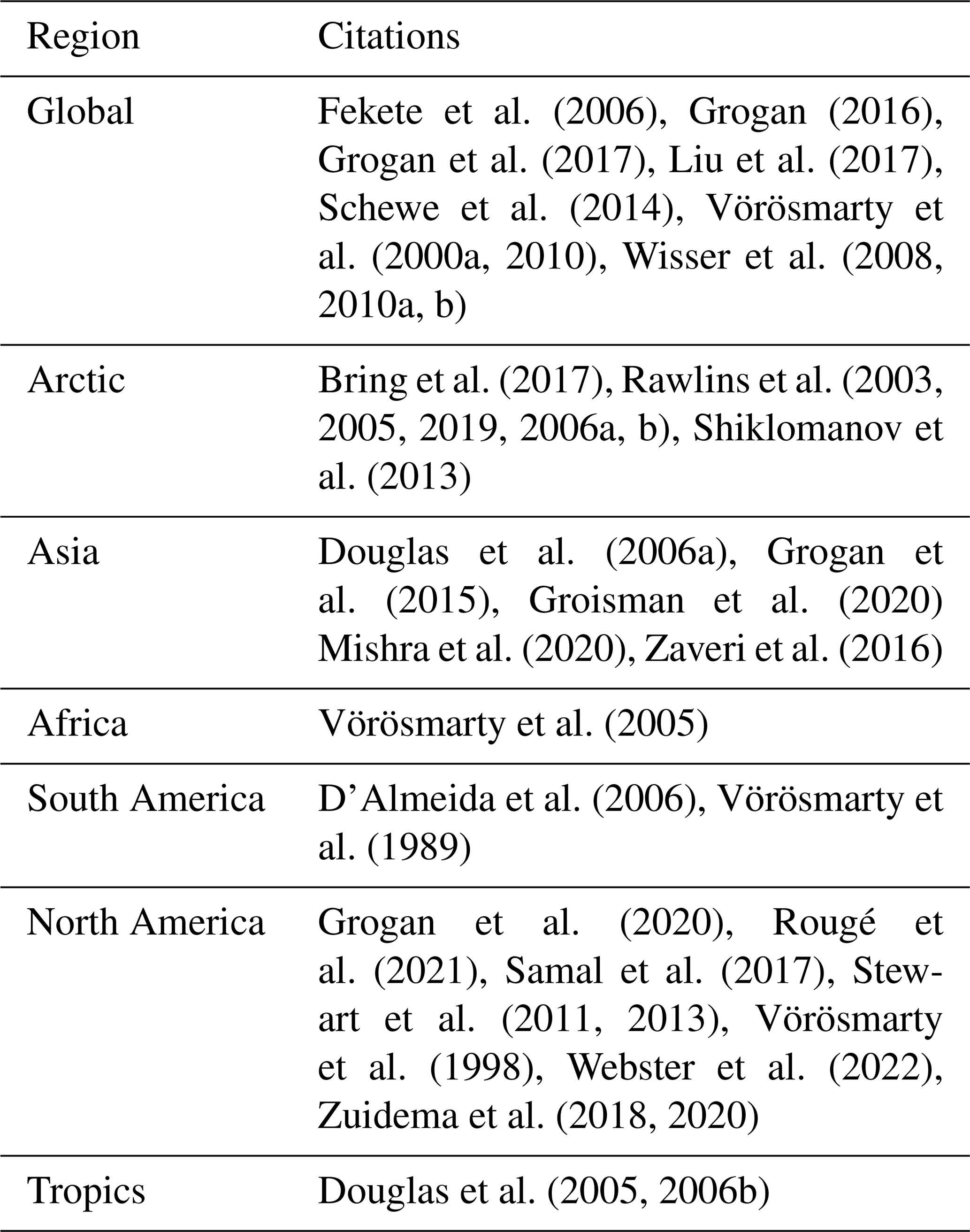
WBM v.1.0.0 is open source and distributed under the terms of the GNU Public License version 3, as published by the Free Software Foundation. Model code is provided in a GitHub repository: https://github.com/wsag/WBM (last access: 10 March 2022), and release v.1.0.0 is archived on Zenodo (Grogan and Zuidema, 2022, https://doi.org/10.5281/zenodo.6263097). Input data required to reproduce the simulations presented here that cannot be downloaded directly from other sources due to either lack of availability or substantial pre-processing requirements for use in WBM v.1.0.0 (see Table 4) are provided for download here: https://wbm.unh.edu/ (last access: 4 March 2022; Grogan et al., 2022, https://doi.org/10.34051/d/2022.2). The GitHub repository will be updated as bug fixes, new modules, and further development occurs. Development and maintenance of the main branch of the WBM continues at the University of New Hampshire, and we welcome contributions from other parties.
The supplement related to this article is available online at: https://doi.org/10.5194/gmd-15-7287-2022-supplement.
DSG contributed to conceptualization, methodology, formal analysis, validation/evaluation, visualization, and original draft writing. SZ contributed to software development, data curation, and draft writing. AP contributed to software development (lead developer), investigation, data curation, and draft writing. SG contributed to software development, investigation, and data curation. RBL contributed to conceptualization, funding acquisition, project administration, supervision, writing – review and editing. WMW contributed to funding acquisition, project administration, supervision, and writing – review and editing.
The contact author has declared that none of the authors has any competing interests.
Publisher's note: Copernicus Publications remains neutral with regard to jurisdictional claims in published maps and institutional affiliations.
We thank the many researchers, students, and staff at UNH and other institutions who have made contributions to WBM over the years. We also thank the six anonymous referees for improving this paper.
This research has been supported by: The U.S. Department of Energy, Office of Science, Biological and Environmental Research Program, Earth and Environmental Systems Modeling, MultiSector Dynamics (grant no. DE-SC005171 and cooperative agreements DE-SC0016162 and DE-SC0022141), the National Science Foundation Division of Earth Sciences (grant no. 1038818), Division of Social and Economic Sciences (grant no. 1639524), Division of Chemical, Bioengineering, Environmental, and Transport Systems (grant no. 1855937), Division of Behavioral and Cognitive Sciences (grant no. 1114851), NH EPSCoR New England Sustainability Consortium (grant no. EPS-1330641), NH EPSCoR Ecosystems and Society (grant no. EPS-1101245), the Plum Island Long Term Ecological Research site (grant no. OCE-1637630), the Graduate Research Fellowship Program (grant no. DGE-0913620), The National Aeronautical and Space Administration, Earth Science Division's High Mountain Asia program (grant nos. NNX17AB28G and 80NSSC20K1595), the Earth Science Division's Sea Level Change program (grant no. 80NSSC20K1296), the United States Environmental Protection Agency, Science to Achieve Results (grant no. R836169), and the Swedish funding agency Formas (grant no. 2017-00,608).
This paper was edited by Charles Onyutha and reviewed by six anonymous referees.
Aber, J. D., Ollinger, S. V., and Driscoll, C. T.: Modeling nitrogen saturation in forest ecosystems in response to land use and atmospheric deposition, Ecol. Model., 101, 61–78, https://doi.org/10.1016/S0304-3800(97)01953-4, 1997.
Alexander, R. B., Boyer, E. W., Smith, R. A., Schwarz, G. E., and Moore, R. B.: The Role of Headwater Streams in Downstream Water Quality1: The Role of Headwater Streams in Downstream Water Quality, J. Am. Water Resour. As., 43, 41–59, https://doi.org/10.1111/j.1752-1688.2007.00005.x, 2007.
Allen, R. G., Pereira, L. S., Raes, D., and Smith, M.: FAO Irrigation and drainage paper No. 56, Food and Agriculture Organization of the United Nations, Rome, 56, e156, http://www.climasouth.eu/sites/default/files/FAO%2056.pdf (last access: 20 June 2018), 1998.
Alley, W. M. and Veenhuis, J. E.: Effective Impervious Area in Urban Runoff Modeling, J. Hydraul. Eng., 109, 313–319, https://doi.org/10.1061/(ASCE)0733-9429(1983)109:2(313), 1983.
Biemans, H. and Siderius, C.: Advances in global hydrology – crop modelling to support the UN's Sustainable Development Goals in South Asia, Curr. Opin. Env. Sust., 40, 108–116, https://doi.org/10.1016/j.cosust.2019.10.005, 2019.
Blunden, J. and Arndt, D. S.: State of the Climate in 2019, B. Am. Meteorol. Soc., 101, S1–S429, https://doi.org/10.1175/2020BAMSStateoftheClimate.1, 2020.
Bosmans, J. H. C., van Beek, L. P. H., Sutanudjaja, E. H., and Bierkens, M. F. P.: Hydrological impacts of global land cover change and human water use, Hydrol. Earth Syst. Sci., 21, 5603–5626, https://doi.org/10.5194/hess-21-5603-2017, 2017.
Bring, A., Shiklomanov, A., and Lammers, R. B.: Pan-Arctic river discharge: Prioritizing monitoring of future climate change hot spots: PAN-ARCTIC RIVER DISCHARGE MONITORING, Earth's Future, 5, 72–92, https://doi.org/10.1002/2016EF000434, 2017.
Clark, M. P., Nijssen, B., Lundquist, J. D., Kavetski, D., Rupp, D. E., Woods, R. A., Freer, J. E., Gutmann, E. D., Wood, A. W., Brekke, L. D., and Arnold, J. R.: A unified approach for process-based hydrologic modeling: 1. Modeling concept, Water Resour. Res., 51, 2498–2514, https://doi.org/10.1002/2015WR017198, 2015.
Cohen, S., Kettner, A. J., Syvitski, J. P. M., and Fekete, B. M.: WBMsed, a distributed global-scale riverine sediment flux model: Model description and validation, Comput. Geosci., 53, 80–93, https://doi.org/10.1016/j.cageo.2011.08.011, 2013.
Cohen, S., Kettner, A. J., and Syvitski, J. P. M.: Global suspended sediment and water discharge dynamics between 1960 and 2010: Continental trends and intra-basin sensitivity, Global Planet. Change, 115, 44–58, https://doi.org/10.1016/j.gloplacha.2014.01.011, 2014.
Cohen, S., Praskievicz, S., and Maidment, D. R.: Featured Collection Introduction: National Water Model, J. Am. Water Resour. As., 54, 767–769, https://doi.org/10.1111/1752-1688.12664, 2018.
Dai, A. and Trenberth, K. E.: Estimates of freshwater discharge from continents: Latitudinal and seasonal variations, J. Hydrometeorol., 3, 660–687, https://doi.org/10.1175/1525-7541(2002)003<0660:EOFDFC>2.0.CO;2, 2002.
Dalin, C., Wada, Y., Kastner, T., and Puma, M. J.: Groundwater depletion embedded in international food trade, Nature, 543, 700–704, https://doi.org/10.1038/nature21403, 2017.
D'Almeida, C., Vörösmarty, C. J., Marengo, J. A., Hurtt, G. C., Dingman, S. L., and Keim, B. D.: A water balance model to study the hydrological response to different scenarios of deforestation in Amazonia, J. Hydrol., 331, 125–136, https://doi.org/10.1016/j.jhydrol.2006.05.027, 2006.
Deardorff, J. W.: Efficient prediction of ground surface temperature and moisture, with inclusion of a layer of vegetation, J. Geophys. Res., 83, 1889, https://doi.org/10.1029/JC083iC04p01889, 1978.
de Wit, M. J. M.: Nutrient fluxes at the river basin scale. I: the PolFlow model, Hydrol. Process., 15, 743–759, https://doi.org/10.1002/hyp.175, 2001.
Dickinson, R. E.: Modeling evapotranspiration for three-dimensional global climate models, in: Geophysical Monograph Series, edited by: Hansen, J. E. and Takahashi, T., American Geophysical Union, 29, 58–72, Washington, D.C., https://doi.org/10.1029/GM029p0058, 1984.
Dillon, P., Stuyfzand, P., Grischek, T., Lluria, M., Pyne, R. D. G., Jain, R. C., Bear, J., Schwarz, J., Wang, W., Fernandez, E., and Stefan, C.: Sixty years of global progress in managed aquifer recharge, Hydrogeol. J., 27, 1–30, https://doi.org/10.1007/s10040-018-1841-z, 2019.
Dingman, S. L.: Equilibrium temperatures of water surfaces as related to air temperature and solar radiation, Water Resour. Res., 8, 42–49, https://doi.org/10.1029/WR008i001p00042, 1972.
Dingman, S. L.: Physical hydrology, 2nd edn., Upper Saddle River, N.J, Prentice Hall, 2002.
Dingman, S. L.: Fluvial Hydraulics, Oxford University Press, New York, NY, 2009.
Döll, P. and Siebert, S.: Global modeling of irrigation water requirements: GLOBAL MODELING OF IRRIGATION WATER REQUIREMENTS, Water Resour. Res., 38, 8-1–8-10, https://doi.org/10.1029/2001WR000355, 2002.
Döll, P., Kaspar, F., and Lehner, B.: A global hydrological model for deriving water availability indicators: model testing and validation, J. Hydrol., 270, 105–134, https://doi.org/10.1016/S0022-1694(02)00283-4, 2003.
Döll, P., Hoffmann-Dobrev, H., Portmann, F. T., Siebert, S., Eicker, A., Rodell, M., Strassberg, G., and Scanlon, B. R.: Impact of water withdrawals from groundwater and surface water on continental water storage variations, J. Geodynam., 59–60, 143–156, https://doi.org/10.1016/j.jog.2011.05.001, 2012.
Döll, P., Müller Schmied, H., Schuh, C., Portmann, F. T., and Eicker, A.: Global-scale assessment of groundwater depletion and related groundwater abstractions: Combining hydrological modeling with information from well observations and GRACE satellites, Water Resour. Res., 50, 5698–5720, https://doi.org/10.1002/2014WR015595, 2014.
Dottori, F., Szewczyk, W., Ciscar, J. C., Zhao, F., Alfieri, L., Hirabayashi, Y., Bianchi, A., Mongelli, I., Frieler, K., Betts, R. A., and Feyen, L.: Increased human and economic losses from river flooding with anthropogenic warming, Nat. Clim. Change, 8, 781–786, https://doi.org/10.1038/s41558-018-0257-z, 2018.
Douglas, E. M., Chomitz, K. M., Sebastian, K., Vorosmarty, C. J., and Wood, S.: The Role Of Tropical Forests In Supporting Biodiversity And Hydrological Integrity: A Synoptic Overview, The World Bank, https://doi.org/10.1596/1813-9450-3635, 2005.
Douglas, E. M., Niyogi, D., Frolking, S., Yeluripati, J. B., Pielke Sr., R. A., Niyogi, N., Vörösmarty, C. J., and Mohanty, U. C.: Changes in moisture and energy fluxes due to agricultural land use and irrigation in the Indian Monsoon Belt, Geophys. Res. Lett., 33, L14403, https://doi.org/10.1029/2006GL026550, 2006a.
Douglas, E. M., Wood, S., Sebastian, K., Vörösmarty, C. J., Chomitz, K. M., and Tomich, T. P.: Policy implications of a pan-tropic assessment of the simultaneous hydrological and biodiversity impacts of deforestation, Water Resour. Manag., 21, 211–232, https://doi.org/10.1007/s11269-006-9050-2, 2006b.
Dunn, F. E., Darby, S. E., Nicholls, R. J., Cohen, S., Zarfl, C., and Fekete, B. M.: Projections of declining fluvial sediment delivery to major deltas worldwide in response to climate change and anthropogenic stress, Environ. Res. Lett., 14, 084034, https://doi.org/10.1088/1748-9326/ab304e, 2019.
Eilander, D., van Verseveld, W., Yamazaki, D., Weerts, A., Winsemius, H. C., and Ward, P. J.: A hydrography upscaling method for scale-invariant parametrization of distributed hydrological models, Hydrol. Earth Syst. Sci., 25, 5287–5313, https://doi.org/10.5194/hess-25-5287-2021, 2021.
Elliott, J., Deryng, D., Müller, C., Frieler, K., Konzmann, M., Gerten, D., Glotter, M., Flörke, M., Wada, Y., Best, N., and Eisner, S.: Constraints and potentials of future irrigation water availability on agricultural production under climate change, P. Natl. Acad. Sci. USA, 111, 3239–3244, https://doi.org/10.1073/pnas.1222474110, 2014.
Falkenmark, M. and Rockström, J.: The New Blue and Green Water Paradigm: Breaking New Ground for Water Resources Planning and Management, J. Water Resour. Plann. Manage., 132, 129–132, https://doi.org/10.1061/(ASCE)0733-9496(2006)132:3(129), 2006.
Fan, Y., Chen, Y., He, Q., Li, W., and Wang, Y.: Isotopic Characterization of River Waters and Water Source Identification in an Inland River, Central Asia, Water, 8, 286, https://doi.org/10.3390/w8070286, 2016.
FAO: AQUASTAT Core Database, Food and Agricultural Organization of the United Nations [data set], https://www.fao.org/aquastat/statistics/query/index.html;jsessionid=71F6F6340C470CFBE92D71489546AA39, last access: 1 July 2015.
FAO: AQUASTAT Core Database. Food and Agricultural Organization of the United Nations [data set], https://www.fao.org/aquastat/en/databases/maindatabase, last access: 1 January 2016.
FAO/UNESCO: Digital soil map of the world and derived soil properties, https://www.fao.org/soils-portal/soil-survey/soil-maps-and-databases/faounesco-soil-map-of-the-world/en/ (last access: 15 July 2015), FAO, Rome, Italy, 2003.
Federer, C. A., Vörösmarty, C., and Fekete, B.: Sensitivity of annual evaporation to soil and root properties in two models of contrasting complexity, J. Hydrometeorol., 4, 1276–1290, https://doi.org/10.1175/1525-7541(2003)004<1276:SOAETS>2.0.CO;2, 2003.
Fekete, B. M., Vörösmarty, C. J., and Grabs, W.: Global Composite Runoff Fields on Observed River Discharge and Simulated Water Balances, Technical Report No. 22, Global Runoff Data Center, Koblenz, Germany, 2000.
Fekete, B. M., Vörösmarty, C. J., and Grabs, W.: High-resolution fields of global runoff combining observed river discharge and simulated water balances: HIGH-RESOLUTION COMPOSITE RUNOFF FIELDS, Global Biogeochem. Cycles, 16, 15-1–15-10. https://doi.org/10.1029/1999GB001254, 2002.
Fekete, B. M., Gibson, J. J., Aggarwal, P., and Vörösmarty, C. J.: Application of isotope tracers in continental scale hydrological modeling, J. Hydrol., 330, 444–456, https://doi.org/10.1016/j.jhydrol.2006.04.029, 2006.
Fischer, G., Nachtergaele, F., Prieler, S., van Velthuizen, H. T., Verelst, L., and Wiberg, D.: Global Agro-ecological Zones Assessment for Agriculture (GAEZ 2008), IIASA, Laxenburg, Austria and FAO, Rome, Italy, 2008.
Frenken, K. (Ed.).: Irrigation in Southern and Eastern Asia in figures: Aquastat survey, 2011, Food and Agriculture of the United Nations, Rome, 2012.
The Global Runoff Data Centre: GRDC Reference Dataset, The Global Runoff Data Centre, 56068 Koblenz, Germany [data set], https://www.bafg.de/GRDC/EN/04_spcldtbss/43_GRfN/refDataset_node.html (last access: 4 October 2016), 2015.
The Global Runoff Data Centre: GRDC Reference Dataset, The Global Runoff Data Centre, 56068 Koblenz, Germany [data set], https://www.bafg.de/GRDC/EN/04_spcldtbss/43_GRfN/refDataset_node.html, 2020.
Gelaro, R., McCarty, W., Suárez, M. J., Todling, R., Molod, A., Takacs, L., Randles, C. A., Darmenov, A., Bosilovich, M. G., Reichle, R., and Wargan, K.: The Modern-Era Retrospective Analysis for Research and Applications, Version 2 (MERRA-2), J. Climate, 30, 5419–5454, https://doi.org/10.1175/JCLI-D-16-0758.1, 2017.
Gerten, D., Schlaphoff, S., Haberlandt, U., Lucht, W., and Sitch, S.: Terresterial vegetation and water balance – hydrological evaluation of a dynamic global vegetation model, https://doi.org/10.1016/j.jhydrol.2003.09.029, 2004.
Ghassemi, F. and White, I.: Inter-basin water transfer: case studies from Australia, United States, Canada, China, and India, Cambridge University Press, Cambridge, UK, New York, 2007.
Gleeson, T., Wada, Y., Bierkens, M. F. P., and van Beek, L. P. H.: Water balance of global aquifers revealed by groundwater footprint, Nature, 488, 197–200. https://doi.org/10.1038/nature11295, 2012.
Gleick, P. H., Pacific Institute for Studies in Development, Environment, and Security, and Stockholm Environment Institute (Eds.): Water in crisis: a guide to the world's fresh water resources, Oxford University Press, New York, ISBN-13 978-0195076288, 1993.
Gochis, D. J., Barlage, M., Cabell, R., Casali, M., Dugger, A., FitzGerald, K., McAllister, M., McCreight, J., RafieeiNasab, A., Read, L., Sampson, D., Yates, D., and Zhang, Y.: The WRF-Hydro modeling system technical description, Version 5.1.1, NCAR Technial Note, 107 pp., Zenodo, https://doi.org/10.5281/zenodo.3625238, 2020.
Grafton, R. Q., Williams, J., Perry, C. J., Molle, F., Ringler, C., Steduto, P., Udall, B., Wheeler, S. A., Wang, Y., Garrick, D., and Allen, R. G.: The paradox of irrigation efficiency, Science, 361, 748–750, https://doi.org/10.1126/science.aat9314, 2018.
Grogan, D. S.: Global and Regaional assessments of unsustainable groundwater use in irrigated agriculture, PhD Thesis, University of New Hampshire, USA, 221 pp., 2016.
Grogan, D. S. and Zuidema, S.: wsag/WBM: v1.0.0 (v1.0.0), Zenodo [code], https://doi.org/10.5281/zenodo.6263097, 2022.
Grogan, D. S., Zhang, F., Prusevich, A., Lammers, R. B., Wisser, D., Glidden, S., Li, C., and Frolking, S.: Quantifying the link between crop production and mined groundwater irrigation in China, Sci. Total Environ., 511, 161–175, https://doi.org/10.1016/j.scitotenv.2014.11.076, 2015.
Grogan, D. S., Wisser, D., Prusevich, A., Lammers, R. B., and Frolking, S.: The use and re-use of unsustainable groundwater for irrigation: a global budget, Environ. Res. Lett., 12, 034017, https://doi.org/10.1088/1748-9326/aa5fb2, 2017.
Grogan, D. S., Burakowski, E. A., and Contosta, A. R.: Snowmelt control on spring hydrology declines as the vernal window lengthens, Environ. Res. Lett., 15, 114040, https://doi.org/10.1088/1748-9326/abbd00, 2020.
Grogan, D. S., Zuidema, S., Prusevich, A., Wollheim, W.M., Glidden, S., and Lammers, R. B.: University of New Hampshire Water Balance Model Ancillary Data for use with the WBM Open Source Release Version 1.0.0, University of New Hampshire [data set], https://doi.org/10.34051/d/2022.2, 2022.
Groisman, P. Y., Bulygina, O. N., Henebry, G. M., Speranskaya, N. A., Shiklomanov, A. I., Chen, Y., Tchebakova, N. M., Parfenova, E. I., Tilinina, N. D., Zolina, O. G., and Dufour, A.: Dry Land Belt of Northern Eurasia: Contemporary Environmental Changes, in: Gutman, G., Chen, J., Henebry, G. M., and Kappas, M., Landscape Dynamics of Drylands across Greater Central Asia: People, Societies and Ecosystems, 17, 11–23, Springer International Publishing, Cham, https://doi.org/10.1007/978-3-030-30742-4_2, 2020.
Gupta, H. V., Kling, H., Yilmaz, K. K., and Martinez, G. F.: Decomposition of the mean squared error and NSE performance criteria: Implications for improving hydrological modelling, J. Hydrol., 377, 80–91, https://doi.org/10.1016/j.jhydrol.2009.08.003, 2009.
Haddeland, I., Heinke, J., Biemans, H., Eisner, S., Flörke, M., Hanasaki, N., Konzmann, M., Ludwig, F., Masaki, Y., Schewe, J., and Stacke, T.: Global water resources affected by human interventions and climate change, P. Natl. Acad. Sci. USA, 111, 3251–3256, https://doi.org/10.1073/pnas.1222475110, 2014.
Haie, N. and Keller, A. A.: Effective Efficiency as a Tool for Sustainable Water Resources Management, J. Am. Water Resour. As., 44, 961–968, https://doi.org/10.1111/j.1752-1688.2008.00194.x, 2008.
Håkanson, L.: The importance of lake morphometry and catchment characteristics in limnology – ranking based on statistical analyses, Hydrobiologia, 541, 117–137, https://doi.org/10.1007/s10750-004-5032-7, 2005.
Hamon, W. R.: Computation of direct runoff amount from storm rainfall, Int. Assoc. Sci. Hydrol. Pub., 63, 52–62, 1963.
Hanasaki, N., Kanae, S., Oki, T., Masuda, K., Motoya, K., Shirakawa, N., Shen, Y., and Tanaka, K.: An integrated model for the assessment of global water resources – Part 1: Model description and input meteorological forcing, Hydrol. Earth Syst. Sci., 12, 1007–1025, https://doi.org/10.5194/hess-12-1007-2008, 2008a.
Hanasaki, N., Kanae, S., Oki, T., Masuda, K., Motoya, K., Shirakawa, N., Shen, Y., and Tanaka, K.: An integrated model for the assessment of global water resources – Part 2: Applications and assessments, Hydrol. Earth Syst. Sci., 12, 1027–1037, https://doi.org/10.5194/hess-12-1027-2008, 2008b.
Hanasaki, N., Yoshikawa, S., Pokhrel, Y., and Kanae, S.: A global hydrological simulation to specify the sources of water used by humans, Hydrol. Earth Syst. Sci., 22, 789–817, https://doi.org/10.5194/hess-22-789-2018, 2018.
Haqiqi, I., Grogan, D. S., Hertel, T. W., and Schlenker, W.: Quantifying the impacts of compound extremes on agriculture, Hydrol. Earth Syst. Sci., 25, 551–564, https://doi.org/10.5194/hess-25-551-2021, 2021.
Harrigan, S., Zsoter, E., Alfieri, L., Prudhomme, C., Salamon, P., Wetterhall, F., Barnard, C., Cloke, H., and Pappenberger, F.: GloFAS-ERA5 operational global river discharge reanalysis 1979–present, Earth Syst. Sci. Data, 12, 2043–2060, https://doi.org/10.5194/essd-12-2043-2020, 2020.
Hrachowitz, M., Savenije, H., Bogaard, T. A., Tetzlaff, D., and Soulsby, C.: What can flux tracking teach us about water age distribution patterns and their temporal dynamics?, Hydrol. Earth Syst. Sci., 17, 533–564, https://doi.org/10.5194/hess-17-533-2013, 2013.
Huang, T., Wollheim, W. M., and Jones, S. H.: Removal of Fecal Indicator Bacteria by River Networks, Water, 14, 617, https://doi.org/10.3390/w14040617, 2022.
Huss, M. and Hock, R.: A new model for global glacier change and sea-level rise, Front. Earth Sci., 3, 54, https://doi.org/10.3389/feart.2015.00054, 2015.
Jägermeyr, J., Gerten, D., Heinke, J., Schaphoff, S., Kummu, M., and Lucht, W.: Water savings potentials of irrigation systems: global simulation of processes and linkages, Hydrol. Earth Syst. Sci., 19, 3073–3091, https://doi.org/10.5194/hess-19-3073-2015, 2015.
Jägermeyr, J., Gerten, D., Schaphoff, S., Heinke, J., Lucht, W., and Rockström, J.: Integrated crop water management might sustainably halve the global food gap, Environ. Res. Lett., 11, 025002, https://doi.org/10.1088/1748-9326/11/2/025002, 2016.
Jasechko, S., Perrone, D., Befus, K. M., Bayani Cardenas, M., Ferguson, G., Gleeson, T., Luijendijk, E., McDonnell, J. J., Taylor, R. G., Wada, Y., and Kirchner, J. W.: Global aquifers dominated by fossil groundwaters but wells vulnerable to modern contamination, Nat. Geosci., 10, 425–429, https://doi.org/10.1038/ngeo2943, 2017.
Kadiresan, K. and Khanal, P. R.: Rethinking Irrigation for Global Food Security: Irrigation and food security, Irrig. Drain., 67, 8–11, https://doi.org/10.1002/ird.2219, 2018.
Konar, M., Hussein, Z., Hanasaki, N., Mauzerall, D. L., and Rodriguez-Iturbe, I.: Virtual water trade flows and savings under climate change, Hydrol. Earth Syst. Sci., 17, 3219–3234, https://doi.org/10.5194/hess-17-3219-2013, 2013.
Konikow, L. F.: Contribution of global groundwater depletion since 1900 to sea-level rise, Geophys. Res. Lett., 38, L17401, doi:10.1029/2011GL048604, 2011.
Kumar, S. V., Peters-Lidard, C. D., Tian, Y., Houser, P. R., Geiger, J., Olden, S., Lighty, L., Eastman, J. L., Doty, B., Dirmeyer, P., and Adams, J.: Land information system: An interoperable framework for high resolution land surface modeling, Environ. Model. Softw., 21, 1402–1415, https://doi.org/10.1016/j.envsoft.2005.07.004, 2006.
Lawrence, D. M., Fisher, R. A., Koven, C. D., Oleson, K. W., Swenson, S. C., Bonan, G., Collier, N., Ghimire, B., van Kampenhout, L., Kennedy, D., and Kluzek, E.: The Community Land Model Version 5: Description of New Features, Benchmarking, and Impact of Forcing Uncertainty, J. Adv. Model. Earth Sy., 11, 4245–4287, https://doi.org/10.1029/2018MS001583, 2019.
Lehner, B., Verdin, K., and Jarvis, A.: New Global Hydrography Derived From Spaceborne Elevation Data, Eos, Transactions American Geophysical Union, 89, 93–94, https://doi.org/10.1029/2008EO100001, 2008.
Lehner, B., Liermann, C. R., Revenga, C., Vörösmarty, C., Fekete, B., Crouzet, P., Döll, P., Endejan, M., Frenken, K., Magome, J., and Nilsson, C.: High-resolution mapping of the world's reservoirs and dams for sustainable river-flow management, Front. Ecol. Environ., 9, 494–502, https://doi.org/10.1890/100125, 2011.
Leopold, L. B. and Maddock, T.: The Hydraulic Geometry of Stream Channels and Some Physiographic Implications, United States Geological Survey, Professional Paper 252, 57 pp., https://doi.org/10.3133/pp252, 1953.
Liang, S. and Greene, R.: A high-resolution global runoff estimate based on GIS and an empirical runoff coefficient, Hydrol. Res., 51, 1238–1260, https://doi.org/10.2166/nh.2020.132, 2020.
Liang, X., Lettenmaier, D. P., Wood, E. F., and Burges, S. J.: A simple hydrologically based model of land surface water and energy fluxes for general circulation models, J. Geophys. Res., 99, 14415–14428, https://doi.org/10.1029/94JD00483, 1994.
Lin, P., Pan, M., Beck, H. E., Yang, Y., Yamazaki, D., Frasson, R., David, C. H., Durand, M., Pavelsky, T. M., Allen, G. H., Gleason, C. J., and Wood, E. F.: Global Reconstruction of Naturalized River Flows at 2.94 Million Reaches, Water Resour. Res., 55, 6499–6516, https://doi.org/10.1029/2019WR025287, 2019.
Liu, J., Hertel, T. W., Lammers, R. B., Prusevich, A., Baldos, U. L. C., Grogan, D. S., and Frolking, S.: Achieving sustainable irrigation water withdrawals: global impacts on food security and land use, Environ. Res. Lett., 12, 104009, https://doi.org/10.1088/1748-9326/aa88db, 2017.
Maidment, D. R. (Ed.): Handbook of hydrology, McGraw-Hill, New York, ISBN-13 978-0070397323 , 1993.
Miara, A. and Vörösmarty, C. J.: A dynamic model to assess tradeoffs in power production and riverine ecosystem protection, Environ. Sci.-Process. Impacts, 15, 1113–1126, https://doi.org/10.1039/C3EM00196B, 2013.
Miara, A., Macknick, J. E., Vörösmarty, C. J., Tidwell, V. C., Newmark, R., and Fekete, B.: Climate and water resource change impacts and adaptation potential for US power supply, Nat. Clim. Change, 7, 793–798, https://doi.org/10.1038/nclimate3417, 2017.
Mineau, M. M., Wollheim, W. M., and Stewart, R. J.: An index to characterize the spatial distribution of land use within watersheds and implications for river network nutrient removal and export, Geophys. Res. Lett., 42, 6688–6695, https://doi.org/10.1002/2015GL064965, 2015.
Mishra, S. K., Veselka, T. D., Prusevich, A. A., Grogan, D. S., Lammers, R. B., Rounce, D. R., Ali, S. H., and Christian, M. H.: Differential Impact of Climate Change on the Hydropower Economics of Two River Basins in High Mountain Asia, Front. Environ. Sci., 8, 26, https://doi.org/10.3389/fenvs.2020.00026, 2020.
Monteith, J. L.: Evaporation and environment, Symposia of the Society for Experimental Biology, 19, 205–234, 1965.
Mulholland, P. J., Helton, A. M., Poole, G. C., Hall, R. O., Hamilton, S. K., Peterson, B. J., Tank, J. L., Ashkenas, L. R., Cooper, L. W., Dahm, C. N., and Dodds, W. K.: Stream denitrification across biomes and its response to anthropogenic nitrate loading, Nature, 452, 202–205, https://doi.org/10.1038/nature06686, 2008.
Müller Schmied, H., Eisner, S., Franz, D., Wattenbach, M., Portmann, F. T., Flörke, M., and Döll, P.: Sensitivity of simulated global-scale freshwater fluxes and storages to input data, hydrological model structure, human water use and calibration, Hydrol. Earth Syst. Sci., 18, 3511–3538, https://doi.org/10.5194/hess-18-3511-2014, 2014.
Nash, J. E. and Sutcliffe, J. V:. River flow forecasting through conceptual models part I–A discussion of principles, J. Hydrol., 10, 282–290, 1970.
Nijssen, B., O'Donnell, G. M., Lettenmaier, D. P., Lohmann, D., and Wood, E. F.: Predicting the discharge of global rivers, J. Climate, 14, 3307–3323, https://doi.org/10.1175/1520-0442(2001)014<3307:PTDOGR>2.0.CO;2, 2001.
Niswonger, R. G., Morway, E. D., Triana, E., and Huntington, J. L.: Managed aquifer recharge through off-season irrigation in agricultural regions, Water Resour. Res., 53, 6970–6992, https://doi.org/10.1002/2017WR020458, 2017.
Oki, T., Agata, Y., Kanae, S., Saruhashi, T., Yang, D., and Musiake, K.: Global assessment of current water resources using total runoff integrating pathways, Hydrol. Sci. J., 46, 983–995, https://doi.org/10.1080/02626660109492890, 2001.
Park, C. C.: World-wide variations in hydraulic geometry exponents of stream channels: An analysis and some observations, J. Hydrol., 33, 133–146, https://doi.org/10.1016/0022-1694(77)90103-2, 1977.
Penman, H. L.: Natural evaporation from open water, bare soil and grass, P. R. Soc. Lond. A, 193, 120–145, 1948.
Plummer, L. N., Rupert, M. G., Busenberg, E., and Schlosser, P.: Age of Irrigation Water in Ground Water from the Eastern Snake River Plain Aquifer, South-Central Idaho, Ground Water, 38, 264–283, https://doi.org/10.1111/j.1745-6584.2000.tb00338.x, 2000.
Pokhrel, Y., Hanasaki, N., Koirala, S., Cho, J., Yeh, P. J. F., Kim, H., Kanae, S., and Oki, T.: Incorporating Anthropogenic Water Regulation Modules into a Land Surface Model, J. Hydrometeorol., 13, 255–269, https://doi.org/10.1175/JHM-D-11-013.1, 2012.
Portmann, F. T., Siebert, S., and Döll, P.: MIRCA2000-Global monthly irrigated and rainfed crop areas around the year 2000: A new high-resolution data set for agricultural and hydrological modeling: MONTHLY IRRIGATED AND RAINFED CROP AREAS, Global Biogeochem. Cycles, 24, 1, https://doi.org/10.1029/2008GB003435, 2010.
Prusevich, A., Lammers, R., and Grogan, D.: High Mountain Asia Rasterized PyGEM Glacier Projections with RCP Scenarios, NASA National Snow and Ice Data Center DAAC [data set], https://doi.org/10.5067/H118TCMSUH3Q, 2021.
Rajib, A., Golden, H. E., Lane, C. R., and Wu, Q.: Surface Depression and Water Storage Improves Major River Basin Hydrologic Predictions, Water Resour. Res., 56, 7, https://doi.org/10.1029/2019WR026561, 2020.
Rawlins, M. A.: Increasing freshwater and dissolved organic carbon flows to Northwest Alaska's Elson lagoon, Environ. Res. Lett., 16, 105014, https://doi.org/10.1088/1748-9326/ac2288, 2021.
Rawlins, M. A., Lammers, R. B., Frolking, S., Fekete, B. M., and Vorosmarty, C. J.: Simulating pan-Arctic runoff with a macro-scale terrestrial water balance model, Hydrol. Process., 17, 2521–2539, https://doi.org/10.1002/hyp.1271, 2003.
Rawlins, M. A., McDonald, K. C., Frolking, S., Lammers, R. B., Fahnestock, M., Kimball, J. S., and Vörösmarty, C. J.: Remote sensing of snow thaw at the pan-Arctic scale using the SeaWinds scatterometer, J. Hydrol., 312, 294–311, https://doi.org/10.1016/j.jhydrol.2004.12.018, 2005.
Rawlins, M. A., Frolking, S., Lammers, R. B., and Vörösmarty, C. J.: Effects of Uncertainty in Climate Inputs on Simulated Evapotranspiration and Runoff in the Western Arctic, Earth Interactions, 10, 1–18, https://doi.org/10.1175/EI182.1, 2006a.
Rawlins, M. A., Willmott, C. J., Shiklomanov, A., Linder, E., Frolking, S., Lammers, R. B., and Vörösmarty, C. J.: Evaluation of trends in derived snowfall and rainfall across Eurasia and linkages with discharge to the Arctic Ocean, Geophys. Res. Lett., 33, L07403, https://doi.org/10.1029/2005GL025231, 2006b.
Rawlins, M. A., Cai, L., Stuefer, S. L., and Nicolsky, D.: Changing characteristics of runoff and freshwater export from watersheds draining northern Alaska, The Cryosphere, 13, 3337–3352, https://doi.org/10.5194/tc-13-3337-2019, 2019.
Rawlins, M. A., Connolly, C. T., and McClelland, J. W.: Modeling Terrestrial Dissolved Organic Carbon Loading to Western Arctic Rivers, J. Geophys. Res.-Biogeo., 126, e2021JG006420, https://doi.org/10.1029/2021JG006420, 2021.
Rimsaite, R., Fisher-Vanden, K., Olmstead, S., and Grogan, D. S.: How Well Do U.S. Western Water Markets Convey Economic Information?, Land Economics, 97, 1–16, https://doi.org/10.3368/wple.97.1.050719-0061R, 2021.
Rosegrant, M. W. and Cai, X.: Global Water Demand and Supply Projections: Part 2. Results and Prospects to 2025, Water Int., 27, 170–182, https://doi.org/10.1080/02508060208686990, 2002.
Rost, S., Gerten, D., Bondeau, A., Lucht, W., Rohwer, J., and Schaphoff, S.: Agricultural green and blue water consumption and its influence on the global water system: GLOBAL WATER USE IN AGRICULTURE, Water Resour. Res., 44, 9, https://doi.org/10.1029/2007WR006331, 2008.
Rougé, C., Reed, P. M., Grogan, D. S., Zuidema, S., Prusevich, A., Glidden, S., Lamontagne, J. R., and Lammers, R. B.: Coordination and control – limits in standard representations of multi-reservoir operations in hydrological modeling, Hydrol. Earth Syst. Sci., 25, 1365–1388, https://doi.org/10.5194/hess-25-1365-2021, 2021.
Rounce, D. R., Hock, R., and Shean, D. E.: Glacier Mass Change in High Mountain Asia Through 2100 Using the Open-Source Python Glacier Evolution Model (PyGEM), Front. Earth Sci., 7, 331, https://doi.org/10.3389/feart.2019.00331, 2020a.
Rounce, D. R., Khurana, T., Short, M. B., Hock, R., Shean, D. E., and Brinkerhoff, D. J.: Quantifying parameter uncertainty in a large-scale glacier evolution model using Bayesian inference: application to High Mountain Asia, J. Glaciol., 66, 175–187, https://doi.org/10.1017/jog.2019.91, 2020b.
Sadegh, M. and Vrugt, J. A.: Bridging the gap between GLUE and formal statistical approaches: approximate Bayesian computation, Hydrol. Earth Syst. Sci., 17, 4831–4850, https://doi.org/10.5194/hess-17-4831-2013, 2013.
Saha, S., Moorthi, S., Wu, X., Wang, J., Nadiga, S., Tripp, P., Behringer, D., Hou, Y. T., Chuang, H. Y., Iredell, M., and Ek, M.: The NCEP Climate Forecast System Version 2, J. Climate, 27, 2185–2208, https://doi.org/10.1175/JCLI-D-12-00823.1, 2014.
Samal, N. R., Wollheim, W. M., Zuidema, S., Stewart, R. J., Zhou, Z., Mineau, M. M., Borsuk, M. E., Gardner, K. H., Glidden, S., Huang, T., and Lutz, D. A.: A coupled terrestrial and aquatic biogeophysical model of the Upper Merrimack River watershed, New Hampshire, to inform ecosystem services evaluation and management under climate and land-cover change, Ecol. Soc., 22, 18, https://doi.org/10.5751/ES-09662-220418, 2017.
Schewe, J., Heinke, J., Gerten, D., Haddeland, I., Arnell, N. W., Clark, D. B., Dankers, R., Eisner, S., Fekete, B. M., Colón-González, F. J., and Gosling, S. N.: Multimodel assessment of water scarcity under climate change, P. Natl. Acad. Sci. USA, 111, 3245–3250, https://doi.org/10.1073/pnas.1222460110, 2014.
Shiklomanov, A. I., Lammers, R. B., Lettenmaier, D. P., Polischuk, Y. M., Savichev, O. G., Smith, L. C., and Chernokulsky, A. V.: Hydrological Changes: Historical Analysis, Contemporary Status, and Future Projections, in: Regional Environmental Changes in Siberia and Their Global Consequences, edited by: Groisman, P. Ya. and Gutman, G., Springer Netherlands, Dordrecht, 111–154, https://doi.org/10.1007/978-94-007-4569-8_4, 2013.
Siebert, S. and Döll, P.: Quantifying blue and green virtual water contents in global crop production as well as potential production losses without irrigation, J. Hydrol., 384, 198–217, https://doi.org/10.1016/j.jhydrol.2009.07.031, 2010.
Simon, D.: The Impact of Dams on Floods and Nitrogen Flux in the Lamprey River Watershed, NH, MS thesis, University of New Hampshire, United States, 222 pp., 2018.
Stahl, K., Weiler, M., Freudiger, D., Kohn, I., Seibert, J., Vis, M., Gerlinger, K., and Böhm, M.: Final report to the International Commission for the Hydrology of the Rhine basin (CHR), International Commission for the Hydrology of the Rhine Basin (KHR/CHR), Germany, 22 pp., ISBN 978-90-70980-38-2, 2017.
St Amour, N. A., Gibson, J. J., Edwards, T. W. D., Prowse, T. D., and Pietroniro, A.: Isotopic time-series partitioning of streamflow components in wetland-dominated catchments, lower Liard River basin, Northwest Territories, Canada, Hydrol. Process., 19, 3357–3381, https://doi.org/10.1002/hyp.5975, 2005.
Steinfeld, H., Gerber, P., Wassenaar, T.D., Castel, V., Rosales, M., Rosales, M., and de Haan, C.: Livestock's long shadow: environmental issues and options, Food & Agriculture Org., https://www.fao.org/3/a0701e/a0701e00.htm (last access: 15 March 2021), 2006.
Stewart, R. J., Wollheim, W. M., Gooseff, M. N., Briggs, M. A., Jacobs, J. M., Peterson, B. J., and Hopkinson, C. S.: Separation of river network–scale nitrogen removal among the main channel and two transient storage compartments, Water Resour. Res., 47, 10, https://doi.org/10.1029/2010WR009896, 2011.
Stewart, R. J., Wollheim, W. M., Miara, A., Vörösmarty, C. J., Fekete, B., Lammers, R. B., and Rosenzweig, B.: Horizontal cooling towers: riverine ecosystem services and the fate of thermoelectric heat in the contemporary Northeast US, Environ. Res. Lett., 8, 025010, https://doi.org/10.1088/1748-9326/8/2/025010, 2013.
Sulser, T. B., Ringler, C., Zhu, T., Msangi, S., Bryan, E., and Rosegrant, M. W.: Green and blue water accounting in the Ganges and Nile basins: Implications for food and agricultural policy, J. Hydrol., 384, 276–291, https://doi.org/10.1016/j.jhydrol.2009.10.003, 2010.
Sutanudjaja, E. H., van Beek, R., Wanders, N., Wada, Y., Bosmans, J. H. C., Drost, N., van der Ent, R. J., de Graaf, I. E. M., Hoch, J. M., de Jong, K., Karssenberg, D., López López, P., Peßenteiner, S., Schmitz, O., Straatsma, M. W., Vannametee, E., Wisser, D., and Bierkens, M. F. P.: PCR-GLOBWB 2: a 5 arcmin global hydrological and water resources model, Geosci. Model Dev., 11, 2429–2453, https://doi.org/10.5194/gmd-11-2429-2018, 2018.
Telteu, C.-E., Müller Schmied, H., Thiery, W., Leng, G., Burek, P., Liu, X., Boulange, J. E. S., Andersen, L. S., Grillakis, M., Gosling, S. N., Satoh, Y., Rakovec, O., Stacke, T., Chang, J., Wanders, N., Shah, H. L., Trautmann, T., Mao, G., Hanasaki, N., Koutroulis, A., Pokhrel, Y., Samaniego, L., Wada, Y., Mishra, V., Liu, J., Döll, P., Zhao, F., Gädeke, A., Rabin, S. S., and Herz, F.: Understanding each other's models: an introduction and a standard representation of 16 global water models to support intercomparison, improvement, and communication, Geosci. Model Dev., 14, 3843–3878, https://doi.org/10.5194/gmd-14-3843-2021, 2021.
Tran, D., Kovacs, K., and Wallander, S.: Long run optimization of landscape level irrigation through managed aquifer recharge or expanded surface reservoirs, J. Hydrol., 579, 124220, https://doi.org/10.1016/j.jhydrol.2019.124220, 2019.
Turner, S. W. D., Hejazi, M., Yonkofski, C., Kim, S. H., and Kyle, P.: Influence of Groundwater Extraction Costs and Resource Depletion Limits on Simulated Global Nonrenewable Water Withdrawals Over the Twenty-First Century, Earth's Future, 7, 123–135, https://doi.org/10.1029/2018EF001105, 2019.
United States Army Corps of Engineers: Hydraulic Design of Spillways, 100–111, Coastal and Hydraulics Laboratory, Vicksburg, Mississippi, 1987.
United States Bureau of Reclamation: Design of small dams, 3rd edn., xliii, 860 pp., U.S. Dept. of the Interior Washington, D.C., 1987.
van Beek, L. P. H., Wada, Y., and Bierkens, M. F.: Global monthly water stress: 1. Water balance and water availability, Water Resour. Res., 47, https://doi.org/10.1029/2010WR009791, 2011.
van Beek, L. P. H., Eikelboom, T., Vliet, M. T. H., and Bierkens, M. F. P.: A physically based model of global freshwater surface temperature, Water Resour. Res., 48, 2012WR011819, https://doi.org/10.1029/2012WR011819, 2012.
Van Kirk, R. W., Contor, B. A., Morrisett, C. N., Null, S. E., and Loibman, A. S.: Potential for Managed Aquifer Recharge to Enhance Fish Habitat in a Regulated River, Water, 12, 673, https://doi.org/10.3390/w12030673, 2020.
Veldkamp, T. I. E., Zhao, F., Ward, P. J., de Moel, H., Aerts, J. C. J. H., Müller Schmied, H., Portmann, F. T., Masaki, Y., Pokhrel, Y., Liu, X., Satoh, Y., Gerten, D., Gosling, S. N., Zaherpour, J., and Wada, Y.: Human impact parameterizations in global hydrological models improve estimates of monthly discharges and hydrological extremes: a multi-model validation study, Environ. Res. Lett., 13, 055008, https://doi.org/10.1088/1748-9326/aab96f, 2018.
Vörösmarty, C. J., Moore III, B., Grace, A. L., Gildea, M. P., Melillo, J. M., Peterson, B. J., Rastetter, E. B., and Steudler, P. A.: Continental scale models of water balance and fluvial transport: An application to South America, Global Biogeochem. Cycles, 3, 241–265, https://doi.org/10.1029/GB003i003p00241, 1989.
Vörösmarty, C. J., Federer, C. A., and Schloss, A. L.: Potential evaporation functions compared on US watersheds: Possible implications for global-scale water balance and terrestrial ecosystem modeling, J. Hydrol., 207, 147–169, https://doi.org/10.1016/S0022-1694(98)00109-7, 1998.
Vörösmarty, C. J., Fekete, B. M., Meybeck, M., and Lammers, R. B.: Geomorphometric attributes of the global system of rivers at 30-minute spatial resolution, J. Hydrol., 237, 17–39, https://doi.org/10.1016/S0022-1694(00)00282-1, 2000a.
Vörösmarty, C. J., Green, P., Salisbury, J., and Lammers, R. B.: Global Water Resources: Vulnerability from Climate Change and Population Growth, Science, 289, 284–288, https://doi.org/10.1126/science.289.5477.284, 2000b.
Vörösmarty, C. J., Douglas, E. M., Green, P. A., and Revenga, C.: Geospatial Indicators of Emerging Water Stress: An Application to Africa, AMBIO: A Journal of the Human Environment, 34, 230–236, https://doi.org/10.1579/0044-7447-34.3.230, 2005.
Vörösmarty, C. J., McIntyre, P. B., Gessner, M. O., Dudgeon, D., Prusevich, A., Green, P., Glidden, S., Bunn, S. E., Sullivan, C. A., Liermann, C. R., and Davies, P. M.: Global threats to human water security and river biodiversity, Nature, 467, 555–561, https://doi.org/10.1038/nature09440, 2010.
Wada, Y., van Beek, L. P. H., and Bierkens, M. F. P.: Modelling global water stress of the recent past: on the relative importance of trends in water demand and climate variability, Hydrol. Earth Syst. Sci., 15, 3785–3808, https://doi.org/10.5194/hess-15-3785-2011, 2011.
Wada, Y., van Beek, L. P. H., and Bierkens, M. F. P.: Nonsustainable groundwater sustaining irrigation: A global assessment: NONSUSTAINABLE GROUNDWATER SUSTAINING IRRIGATION, Water Resour. Res., 48, https://doi.org/10.1029/2011WR010562, 2012.
Wada, Y., Wisser, D., and Bierkens, M. F. P.: Global modeling of withdrawal, allocation and consumptive use of surface water and groundwater resources, Earth Syst. Dynam., 5, 15–40, https://doi.org/10.5194/esd-5-15-2014, 2014.
Wada, Y., Lo, M.-H., Yeh, P. J.-F., Reager, J. T., Famiglietti, J. S., Wu, R.-J., and Tseng, Y.-H.: Fate of water pumped from underground and contributions to sea-level rise, Nat. Clim. Change, 6, 777–780, https://doi.org/10.1038/nclimate3001, 2016.
Wada, Y., Bierkens, M. F. P., de Roo, A., Dirmeyer, P. A., Famiglietti, J. S., Hanasaki, N., Konar, M., Liu, J., Müller Schmied, H., Oki, T., Pokhrel, Y., Sivapalan, M., Troy, T. J., van Dijk, A. I. J. M., van Emmerik, T., Van Huijgevoort, M. H. J., Van Lanen, H. A. J., Vörösmarty, C. J., Wanders, N., and Wheater, H.: Human–water interface in hydrological modelling: current status and future directions, Hydrol. Earth Syst. Sci., 21, 4169–4193, https://doi.org/10.5194/hess-21-4169-2017, 2017.
Webster, M., Fisher-Vanden, K., Kumar, V., Lammers, R. B., and Perla, J.: Integrated hydrological, power system and economic modelling of climate impacts on electricity demand and cost, Nat. Energ., 7, 163–169, https://doi.org/10.1038/s41560-021-00958-8, 2022.
Weiler, M., Seibert, J., and Stahl, K.: Magic components-why quantifying rain, snowmelt, and icemelt in river discharge is not easy, Hydrol. Process., 32, 160–166, https://doi.org/10.1002/hyp.11361, 2018.
Widén-Nilsson, E.: Global-Scale Modelling of the Land-Surface Water Balance: Development and Analysis of WASMOD-M, PhD Thesis, Acta Universitatis Upsaliensis, Uppsala, Sweden, 76 pp., 2007.
Willmott, C. J.: ON THE VALIDATION OF MODELS, Phys. Geogr., 2, 184–194, https://doi.org/10.1080/02723646.1981.10642213, 1981.
Willmott, C. J. and Matsuura, K.: Terrestrial Air Temperature and Precipitation: Monthly and Annual Time Series (1950–1999) (Version 2.01), Center for Climatic Research, Department of Geography, University of Delaware [data set], http://climate.geog.udel.edu/~climate/html_pages/download.html (last access: 6 February 2015), 2001.
Willmott, C. J., Rowe, C. M., and Mintz, Y.: Climatology of the terrestrial seasonal water cycle, J. Climatol., 5, 589–606, https://doi.org/10.1002/joc.3370050602, 1985.
Wisser, D., Frolking, S., Douglas, E. M., Fekete, B. M., Vörösmarty, C. J., and Schumann, A. H.: Global irrigation water demand: Variability and uncertainties arising from agricultural and climate data sets, Geophys. Res. Lett., 35, L24408, https://doi.org/10.1029/2008GL035296, 2008.
Wisser, D., Fekete, B. M., Vörösmarty, C. J., and Schumann, A. H.: Reconstructing 20th century global hydrography: a contribution to the Global Terrestrial Network- Hydrology (GTN-H), Hydrol. Earth Syst. Sci., 14, 1–24, https://doi.org/10.5194/hess-14-1-2010, 2010a.
Wisser, D., Frolking, S., Douglas, E. M., Fekete, B. M., Schumann, A. H., and Vörösmarty, C. J.: The significance of local water resources captured in small reservoirs for crop production – A global-scale analysis, J. Hydrol., 384, 264–275, https://doi.org/10.1016/j.jhydrol.2009.07.032, 2010b.
Wollheim, W., Peterson, B. J., Thomas, S. M., Hopkinson, C. H., and Vörösmarty, C. J.: Dynamics of N removal over annual time periods in a suburban river network, J. Geophys. Res., 113, G03038, https://doi.org/10.1029/2007JG000660, 2008a.
Wollheim, W., Vörösmarty, C. J., Bouwman, A. F., Green, P., Harrison, J., Linder, E., Peterson, B. J., Seitzinger, S. P., and Syvitski, J. P. M.: Global N removal by freshwater aquatic systems using a spatially distributed, within-basin approach, Global Biogeochem. Cycles, 22, 2, https://doi.org/10.1029/2007GB002963, 2008b.
Wollheim, W., Stewart, R. J., Aiken, G. R., Butler, K. D., Morse, N. B., and Salisbury, J.: Removal of terrestrial DOC in aquatic ecosystems of a temperate river network, Geophys. Res. Lett., 42, 6671–6679, https://doi.org/10.1002/2015GL064647, 2015.
Wollheim, W. M., Harms, T. K., Peterson, B. J., Morkeski, K., Hopkinson, C. S., Stewart, R. J., Gooseff, M. N., and Briggs, M. A.: Nitrate uptake dynamics of surface transient storage in stream channels and fluvial wetlands, Biogeochemistry, 120, 239–257, https://doi.org/10.1007/s10533-014-9993-y, 2014.
Yamazaki, D., Kanae, S., Kim, H., and Oki, T.: A physically based description of floodplain inundation dynamics in a global river routing model: FLOODPLAIN INUNDATION DYNAMICS, Water Resour. Res., 47, 4, https://doi.org/10.1029/2010WR009726, 2011.
Yamazaki, D., Ikeshima, D., Sosa, J., Bates, P. D., Allen, G. H., and Pavelsky, T. M.: MERIT Hydro: A High-Resolution Global Hydrography Map Based on Latest Topography Dataset, Water Resour. Res., 55, 5053–5073, https://doi.org/10.1029/2019WR024873, 2019.
Yang, Y., Donohue, R. J., and McVicar, T. R.: Global estimation of effective plant rooting depth: Implications for hydrological modeling: GLOBAL HYDROLOGICAL EFFECTIVE ROOTING DEPTH, Water Resour. Res., 52, 8260–8276, https://doi.org/10.1002/2016WR019392, 2016.
Yatagai, A., Kamiguchi, K., Arakawa, O., Hamada, A., Yasutomi, N., and Kitoh, A.: APHRODITE: Constructing a long-term daily gridded precipitation dataset for Asia based on a dense network of rain gauges, B. Am. Meteorol. Soc., 93, 1401–1415, https://doi.org/10.1175/BAMS-D-11-00122.1, 2012.
Zaherpour, J., Gosling, S. N., Mount, N., Müller Schmied, H., Veldkamp, T. I. E., Dankers, R., Eisner, S., Gerten, D., Gudmundsson, L., Haddeland, I., Hanasaki, N., Kim, H., Leng, G., Liu, J., Masaki, Y., Oki, T., Pokhrel, Y., Satoh, Y., Schewe, J., and Wada, Y.: Worldwide evaluation of mean and extreme runoff from six global-scale hydrological models that account for human impacts, Environ. Res. Lett., 13, 065015, https://doi.org/10.1088/1748-9326/aac547, 2018.
Zaveri, E., Grogan, D. S., Fisher-Vanden, K., Frolking, S., Lammers, R. B., Wrenn, D. H., Prusevich, A., and Nicholas, R. E.: Invisible water, visible impact: groundwater use and Indian agriculture under climate change, Environ. Res. Lett., 11, 084005, https://doi.org/10.1088/1748-9326/11/8/084005, 2016.
Zeitoun, M. and Mirumachi, N.: Transboundary water interaction I: reconsidering conflict and cooperation, International Environmental Agreements: Politics, Law and Economics, 8, 297–316, https://doi.org/10.1007/s10784-008-9083-5, 2008.
Zeng, X., Troch, P., Pelletier, J., Niu, G., and Gochis, D.: Development of hybrid 3-D hydrological modeling for the NCAR Community Earth System Model (CESM), Univ. of Arizona Technical Report, United States, https://doi.org/10.2172/1227980, 2015.
Zuidema, S. and Morrison, R.: Hydrologically Consistent Dams Database (version 2.0), Harvard Dataverse [data set], https://doi.org/10.7910/DVN/5YBWWI, 2020.
Zuidema, S., Wollheim, W. M., Mineau, M. M., Green, M. B., and Stewart, R. J.: Controls of Chloride Loading and Impairment at the River Network Scale in New England, J. Environ. Quality, 47, 839–847, https://doi.org/10.2134/jeq2017.11.0418, 2018.
Zuidema, S., Grogan, D., Prusevich, A., Lammers, R., Gilmore, S., and Williams, P.: Interplay of changing irrigation technologies and water reuse: example from the upper Snake River basin, Idaho, USA, Hydrol. Earth Syst. Sci., 24, 5231–5249, https://doi.org/10.5194/hess-24-5231-2020, 2020.
- Abstract
- Introduction
- WBM model description
- Model evaluation
- Water source tracking module demonstration
- Model code
- Discussion
- Conclusions and future work
- Appendix A
- Code and data availability
- Author contributions
- Competing interests
- Disclaimer
- Acknowledgements
- Financial support
- Review statement
- References
- Supplement