MultilayerPy (v1.0): a Python-based framework for building, running and optimising kinetic multi-layer models of aerosols and films

Kinetic multi-layer models of aerosols and films have become the state-of-the-art method of describing complex aerosol processes at the particle and film level. We present MultilayerPy: an open-source framework for building, running and optimising kinetic multi-layer models – namely the kinetic multi-layer model of aerosol surface and bulk chemistry (KM-SUB) and the kinetic multi-layer model of gas–particle interactions in aerosols and clouds (KM-GAP). The modular nature of this package allows the user to iterate through various reaction schemes, diffusion regimes and experimental conditions in a systematic way. In this way, models can be customised and the raw model code itself, produced in a readable way by MultilayerPy, is fully customisable. Optimisation to experimental data using local or global optimisation algorithms is included in the package along with the option to carry out statistical sampling and Bayesian inference of model parameters with a Markov chain Monte Carlo (MCMC) sampler (via the emcee Python package). MultilayerPy abstracts the model building process into separate building blocks, increasing the reproducibility of results and minimising human error. This paper describes the general functionality of MultilayerPy and demonstrates this with use cases based on the oleic- acid–ozone heterogeneous reaction system. The tutorials in the source code (written as Jupyter notebooks) and the documentation aim to encourage users to take advantage of this tool, which is intended to be developed in conjunction with the user base.

1 Introduction

Aerosols are an important atmospheric component and contribute to air quality (indoors and outdoors), public health and the climate (Abbatt and Wang, 2020; Pöschl, 2005). The composition and physical state of aerosols can affect their ability to take up water to form cloud droplets (Schill et al., 2015; Shiraiwa et al., 2011). Understanding how an aerosol particle or film interacts with common atmospheric trace gases, some of which are reactive, affords a better description of atmospheric aerosol processes.

Kinetic multi-layer models of heterogeneous interactions of aerosols with trace gases have become popular in the last decade. In particular, those based on the Pöschl–Rudich–Ammann (PRA) framework (Pöschl et al., 2007) such as the kinetic multi-layer model of surface and bulk chemistry (KM-SUB) (Shiraiwa et al., 2010) and the kinetic multi-layer model of gas–particle interactions (KM-GAP) (Shiraiwa et al., 2012) have been applied in a wide range of studies, providing particle-level insights which are often not possible to obtain experimentally. For example, KM-SUB models have highlighted the impact of crust formation and viscosity on particle and film reaction kinetics, lengthening the chemical lifetime of particle and film constituents with potential impacts on the climate, air pollution and human health (Milsom et al., 2022b; Mu et al., 2018; Pfrang et al., 2011; Zhou et al., 2019). KM-GAP has been coupled with the aerosol inorganic–organic-mixture functional-group activity coefficients (AIOMFAC) thermodynamic model (Zuend et al., 2008, 2011) to calculate equilibration timescales between aerosol particles and surrounding organic and inorganic vapours in a study of liquid–liquid phase separation (Huang et al., 2021).

Software packages facilitating the creation and running of box models (e.g. PyBox, Topping et al., 2018; JlBox, Huang and Topping, 2021; AtChem, Sommariva et al., 2020), aerosol chamber experiments (e.g PyCHAM, O'Meara et al., 2021) and indoor chemistry (INCHEMPy, Shaw and Carslaw, 2021) have recently gained popularity and nurture a more accessible modelling environment, enabling more reproducible and reliable results.

This paper describes MultilayerPy, a package written in Python, which is designed to facilitate the creation and optimisation of kinetic multi-layer models (namely KM-SUB and KM-GAP) in a modular and reproducible way. The key features are presented along with use cases focussing on the well-studied oleic-acid–ozone heterogeneous reaction system (Berkemeier et al., 2021; Gallimore et al., 2017; King et al., 2004, 2020; Milsom et al., 2021b, a, 2022b; Pfrang et al., 2011, 2017; Woden et al., 2021; Zahardis and Petrucci, 2007). An educational tool has recently been created which creates and runs simple kinetic multi-layer models with two reactants (Hua et al., 2022). MultilayerPy is intended for research use and can be used to create and optimise more complex kinetic multi-layer models.

It is envisaged that this paper, along with the accompanying supporting information in the form of Jupyter notebooks in the source code, will encourage new users to use and eventually contribute to this project.

2 Purpose and scientific basis

Currently, the creation of a kinetic multi-layer model requires the researcher to manually construct specific computer code which describes the set of ordinary differential equations (ODEs) which describe the model. For a basic system (e.g. A reacts with B to make C) this method is satisfactory. However, for more complex systems involving many model components, composition-dependent diffusivity and the inverse modelling of experimental data, this manual method quickly becomes cumbersome and prone to human error.

MultilayerPy provides a framework for constructing kinetic multi-layer models so that the model code is produced automatically for the user, removing potential human error in typing out the model code. This code is written in a readable way, enabling the code to be shared with an associated publication and encouraging more reproducible results. This is further supported through the Jupyter notebook (Perkel, 2018), which is a document that incorporates both Python code and markdown text and is gaining popularity as a way of sharing and describing scientific code.

Abstracting the model building, running and optimisation process in this way quickens this time-consuming part of a modelling study and allows the researcher to focus more on the science behind any modelling decisions made. MultilayerPy provides the utility for model parameter evolution via the inclusion of additional user-defined parameters not present in the original model and including time-dependent changes in model parameters (e.g. changes in temperature or the gas phase concentration of a component). There is also scope for model customisation. The model code can be edited and re-incorporated into the MultilayerPy framework. This allows researchers to incorporate conditions or processes which are unique to their specific system.

A challenge at the outset of a modelling study is deciding on a reaction scheme to use. This is illustrated by the modelling of oleic-acid ozonolysis where different reaction schemes have been used in the literature (Berkemeier et al., 2021; Hosny et al., 2016; Shiraiwa et al., 2010). Manually iterating through different reaction schemes can be time consuming. The object-oriented approach of MultilayerPy, where model components are treated as discrete objects, allows the researcher to create and test various model reaction schemes in a few lines of code. Selection of the most suitable model reaction scheme is then feasible.

A detailed description of the KM-SUB and KM-GAP models is presented in their respective publications (Shiraiwa et al., 2010, 2012). Figure 1 illustrates the main concept behind the two models. Essentially, the models split the particle or film into a number of shells or layers. The diffusion of reactants between each layer and the reaction of each component within each layer are resolved. Surface chemistry and the adsorption and desorption of gaseous species are resolved. Additionally, KM-GAP allows the thickness of model layers to change over time, accounting for the evaporation of volatile components in the model and to follow changes in film thickness or particle size during the model run. This means that all model components can partition into and out of the film or particle.

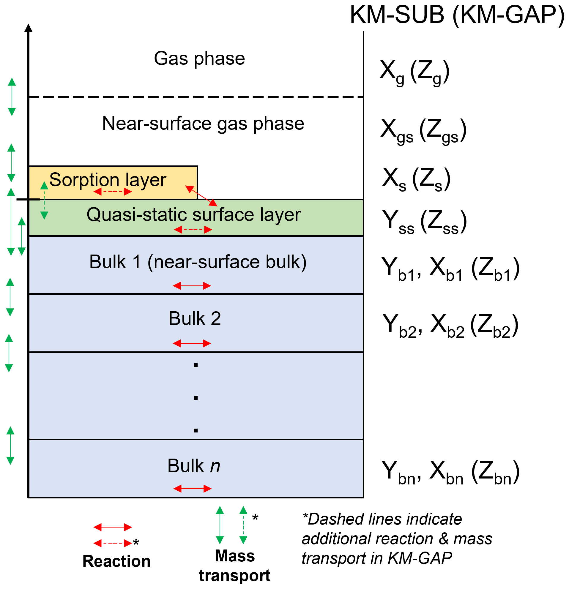
Figure 1 KM-SUB and KM-GAP model visualisation. A particle or film is split into sorption, quasi-static surface and n bulk layers. KM-SUB explicitly splits components into volatile (X) and non-volatile (Y), whereas KM-GAP treats all model components the same, and they are symbolised by Z by convention.

3 MultilayerPy structure and features

MultilayerPy is organised so that different combinations of reaction schemes, diffusion regimes and model types are possible and can be realised in a clear, reproducible way (Fig. 2). This is possible because of the object-oriented programming (OOP) paradigm in which this software is written. Essentially, each component of a multi-layer model is represented by an object (or class) which has its own attributes and methods. The user sets these attributes and uses the methods associated with these objects to carry out model construction, simulation and optimisation. In relatively few lines of code, the user is able to construct this pipeline and run it.

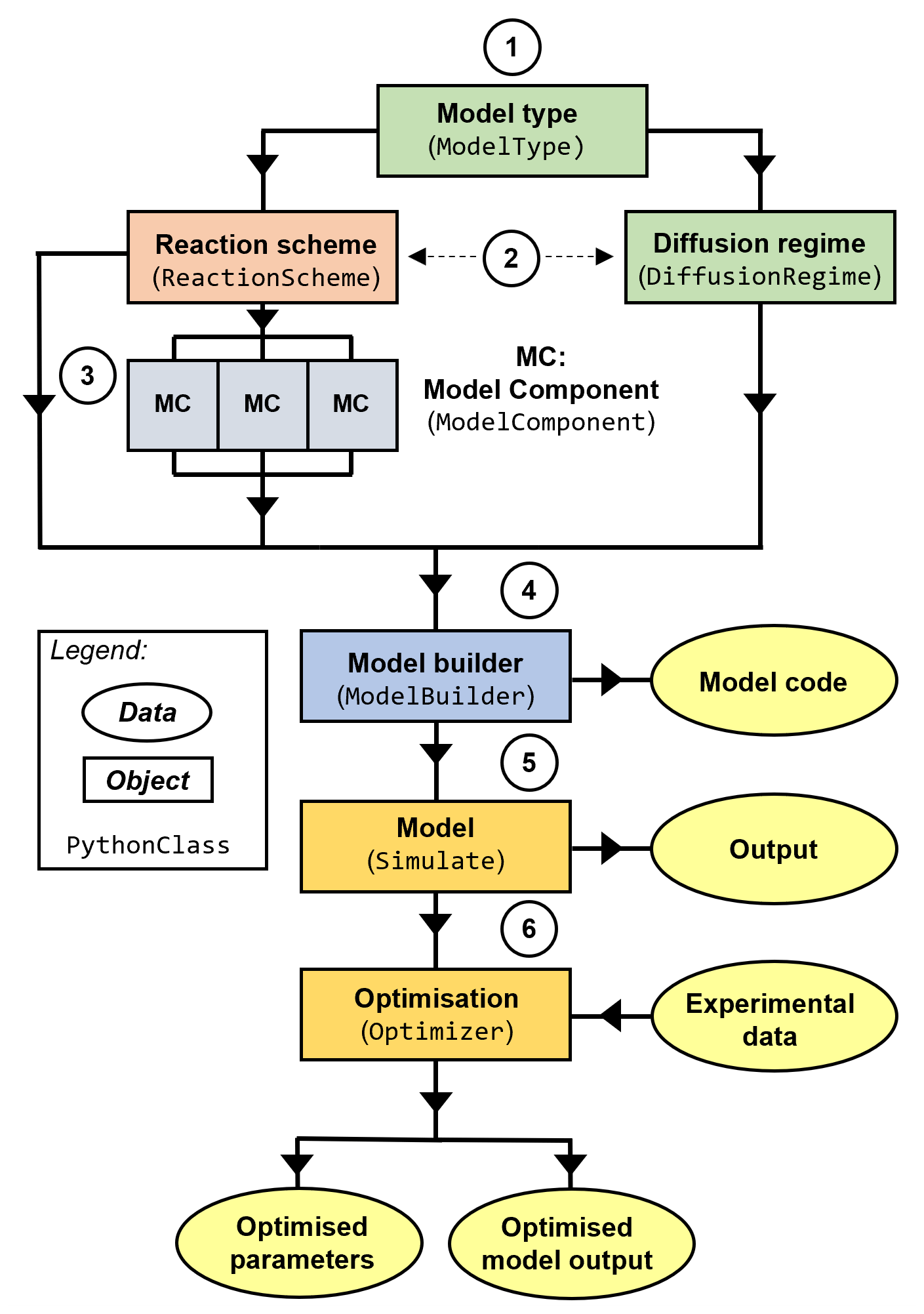
Figure 2 High-level schematic outline of MultilayerPy. Circled numbers correspond to the numbered steps of the model building and optimisation process described in the main text.

Below is an outline of a typical model build, run and optimisation experiment. These steps are expanded on in the subsequent sections:

1. selection of the model type which informs how the model is constructed (KM-SUB or KM-GAP);

2. creation of a reaction scheme and diffusion regime represented in the model – reactions and diffusion regimes (i.e. composition-dependent diffusion) are optional;

3. creation of the model components (chemical species);

4. model construction by combining the reaction scheme, diffusion regime and model components – creation of the model code;

5. model simulator object creation to run and save model outputs – there is potential to add custom model parameterisation (see case study 3);

6. optimisation of the model fit to experimental data, determination of optimised model parameters and optional Markov chain Monte Carlo (MCMC) sampling of the parameter space.

This modular approach to model creation and optimisation is flexible and enables the user to experiment with and iterate through different model designs. One could imagine creating a set of reaction schemes and iterating through them in order to find the one which best describes the data and satisfies the goals of a particular study.

Only a basic knowledge of Python is required to use MultilayerPy and its main features. This is another advantage of abstracting the model building process into the basic building blocks described in Fig. 2.

To encourage new users, the source code for MultilayerPy comes with Jupyter notebooks which provide example uses that can also be used as templates. A good starting point would be to work through the crash course notebook available in the repository. More detailed documentation is included in .html format in the source code along with instructions on how to install and test the package before use in a separate readme file. The easiest way to install the software is to either download the source code from the repository (see the “Code availability” section) or run a pip install as described in the readme. The documentation will be updated with each update to the software.

3.1 Model construction

The first step of model construction is to define the model type and fundamental geometry (spherical particle or planar film). Currently, KM-SUB and KM-GAP models are available in MultilayerPy. Once defined, reaction scheme and diffusion regime are created taking into account the model type and model components, which are instantiated as separate model component objects. It is possible for the user to display the reaction scheme to check that the desired reaction scheme has been defined.

Many reaction schemes, such as the oleic-acid–ozone system, have an uneven product distribution which can be described by a branching ratio. MultilayerPy allows the user to apply a branching ratio to a reaction scheme to account for this.

Composition-dependent bulk diffusion is made possible by the diffusion regime defined by the user. Three different parameterisations are currently available in MultilayerPy: (i) Vignes-type (default) (Vignes, 1966); (ii) obstruction theory (Stroeve, 1975); and (iii) linear combination (Pöschl et al., 2007; Shiraiwa et al., 2010). The evolution of particle diffusivity is of interest to the community and has been highlighted in the kinetic multi-layer modelling and experimental literature (e.g. (semi-) solid crust formation) (Milsom et al., 2021b, a, 2022a; Nash et al., 2006; Pfrang et al., 2011; Zhou et al., 2019). If a simpler well-mixed system is modelled, diffusion evolution as a function of particle composition can be turned off by supplying a “null” argument to the diffusion regime object (see examples in the Jupyter notebooks in the source code repository).

Once the model type, model components, reaction scheme and diffusion regime are defined, the model can be constructed. The building blocks (objects) are supplied to a model builder object. Invoking the build method of this object has two main functions: (i) it writes the model code (ODE function) to a separate .py file, and (ii) it defines a list of required parameters for the model to run (see next section).

The model code defining the system of ODEs for each component in each layer is automatically generated. This is a key utility of MultilayerPy, especially when considering a complex multi-component system. Writing many lines of code manually is error prone. The removal of this risk, along with the readable nature of the model code, enhances the reproducibility and reliability of the results. This file is, however, customisable should the user want to add or remove specific processes in this template framework. Custom modifications should be checked thoroughly.

3.2 Running the model

Once constructed, the model can be run by incorporation into a simulate object, which also requires input model parameters supplied as a Python dictionary. The simulate object can also contain experimental data for optimisation.

Before the model can be run, the number of model bulk layers, initial concentration of each component in each layer, initial layer volume, initial layer surface area and initial layer thickness need to be supplied to the simulate object. MultilayerPy has utility functions which make this process straightforward. The number of model bulk layers is particularly important when modelling viscous systems because bulk diffusion gradients need to be resolved to describe the system sufficiently – the assumption in KM-SUB and KM-GAP models is that each bulk layer is well-mixed.

After running the model for the desired time span the model output, consisting of spatially and temporally resolved number concentration arrays for each model component, is saved and associated with the simulate object. The user can access these outputs easily for further analysis and visualisation.

Simple plotting methods are available which will quickly plot the model output including surface concentrations or the total number of each component in the model as a function of simulation time. Summary heat map plots of component bulk concentrations are also accessible via a plotting function. This allows the user to quickly visualise a model run and decide on the next course of action.

If a KM-GAP model is implemented, the volume, surface area and thickness of each bulk layer as a function of time can be accessed via the simulate object. From this, the user can plot the change in particle diameter and volume as a function of time. An example of this is presented in the corresponding KM-GAP Jupyter notebook in the source code.

Sometimes modification of model input parameters is required. For example, the concentration of a reactive gas can be changed partway through an experiment. This can be implemented in the MultilayerPy framework by supplying a function which changes the concentration of the reactive gas after a certain time point (see the “parameter evolution” Jupyter notebook in the source code for an example). This is possible for any of the model input parameters. Additionally, extra input parameters can be supplied to the model in this manner. These parameters can themselves be optimised.

3.3 Model optimisation

After constructing and running the kinetic multi-layer model, the user may want to optimise the model input parameters. Data can be associated with the simulate object which was created to run the model. Optimisation requires a minimum of a simulate object with data associated with it.

Currently, the built-in cost function is the mean squared error (MSE), which is defined in Eq. (1):

$$\begin{array}{}\text{(1)}& \text{MSE}={\displaystyle \frac{\mathrm{1}}{n}}{\sum }_{i=\mathrm{1}}^n{w}_i(Y_{\text{data},i}-Y_{\text{model},i}{)}^{\mathrm{2}},\end{array}$$

where n is the number of data points and Y_data and Y_model are the experimental and model data points, respectively. A weighting factor (w_i) is applied if there are uncertainties associated with the data and is equivalent to the inverse square of the uncertainty. This is equal to 1 if no uncertainties are provided. The user can supply their own cost function if desired.

There are two main methods of model optimisation available in MultilayerPy: (i) local optimisation (least-squares simplex method); (ii) global optimisation (differential evolution method). Both methods use the implementations found in the SciPy Python package (Virtanen et al., 2020).

Local optimisation is the least computationally expensive way of optimising the model. However, as the name implies, only a local minimum in the cost function will be found (though this could also be the global minimum). This algorithm does not search the entire parameter space looking for a global minimum and will only settle in the nearest local minimum. The user must therefore be confident that the initial model parameters are close to what represents their system.

Global optimisation is more computationally expensive. A description of the Monte Carlo genetic algorithm (MCGA) has been presented by Berkemeier et al. (2017) in the context of kinetic multi-layer modelling (Berkemeier et al., 2017). The implementation in MultilayerPy is similar, with an initial Latin hypercube sampling step (instead of a Monte Carlo sampling step), followed by a differential evolution algorithm implementation which searches the parameter space and applies concepts of natural selection to mutate and select each successive generation of parameter sets (Storn and Price, 1997).

3.4 Estimating parameter uncertainty with a Markov chain Monte Carlo (MCMC) method

A range of model outputs could be considered consistent with experimental data due to the uncertainty associated with each data point. Global optimisation algorithms, such as differential evolution, focus on achieving a single parameter set with the lowest-cost function. However, running the same global optimisation algorithm multiple times can return optimised parameter sets with different values. This is indeed the case with the MCGA algorithm where uncertainties in the optimised parameters are presented as the distribution of optimised parameter values after a set number of MCGA runs (Berkemeier et al., 2017).

MCMC sampling seeks to define the probability distribution for each model parameter by finding the region of highest probability in a given parameter space. First, a parameter set is initiated within pre-defined bounds. Then the parameter set is allowed to “walk” around the parameter space. The likelihood of the next proposed step being accepted is dependent on the likelihood of the current position in the parameter space (i.e. the goodness of the model–data fit). This means that the chain will tend towards regions of higher probability. This is the Markov chain aspect of the MCMC algorithm. The Monte Carlo aspect arises from the randomness associated the proposed next step in the chain, the next sample. When a run is successful, the chain of samples will equilibrate around the region of highest probability. A probability distribution for each varying model parameter can be obtained from the values returned by this equilibrated chain of samples (see Fig. 4c later for an example).

The MCMC algorithm infers the posterior probability distribution function, p(θ|D). This is the probability of the model parameters (θ) given the data (D). This is calculated via Bayes' rule (Eq. 2).

$$\begin{array}{}\text{(2)}& p\left(\mathit{\theta }\mathrm{|}D\right)={\displaystyle \frac{\mathrm{1}}{Z}}p\left(D\mathrm{|}\mathit{\theta }\right)p\left(\mathit{\theta }\right)\end{array}$$

p(θ|D) is proportional to the likelihood (p(D|θ) – essentially the goodness of fit) and the prior probability for the parameters (p(θ)), which is normally set to 1 (uniform) if the prior probability distribution function for each parameter is unknown. The evidence (Z) is a constant which is generally hard to calculate and is ignored in MCMC as it is constant for a given model–experiment system and does not affect the outcome of an MCMC sampling run. Because of this, MCMC cannot be used to select the best of two different models applied to the same data as p(D|θ) would not be normalised to the same scale, although it is possible to compare parameter estimations from different models. For a more detailed description of MCMC sampling and best practices, a paper by Hogg and Foreman-Mackey walks the reader through the algorithm and troubleshoots common problems (Hogg and Foreman-Mackey, 2018).

MultilayerPy employs the well-established emcee python package for MCMC sampling (Foreman-Mackey et al., 2013). This is an ensemble sampler which initiates a number of walkers in the parameter space. The ensemble of walkers can then proceed with the MCMC routine. Parallelisation of the algorithm can be implemented as each walker can be iterated independently. An example of this is given in the “MCMC sampling” Jupyter notebook.

Though MCMC can technically be used as a global optimiser, this is not recommended as there are dedicated global optimisation algorithms which are much more efficient at finding the global minimum, such as the differential evolution algorithm employed in MultilayerPy.

In practice, the model–data system can be optimised (locally or globally) before initiating the walkers in a tight Gaussian “ball” around the optimum point in the parameter space. Initialising the walkers in this way can reduce the time for them to equilibrate. This is the recommended procedure in MultilayerPy and is the way presented in the “MCMC sampling” Jupyter notebook associated with the source code.

An example of how MCMC sampling is implemented in MultilayerPy is presented in the oleic-acid monolayer case study (see case study 2).

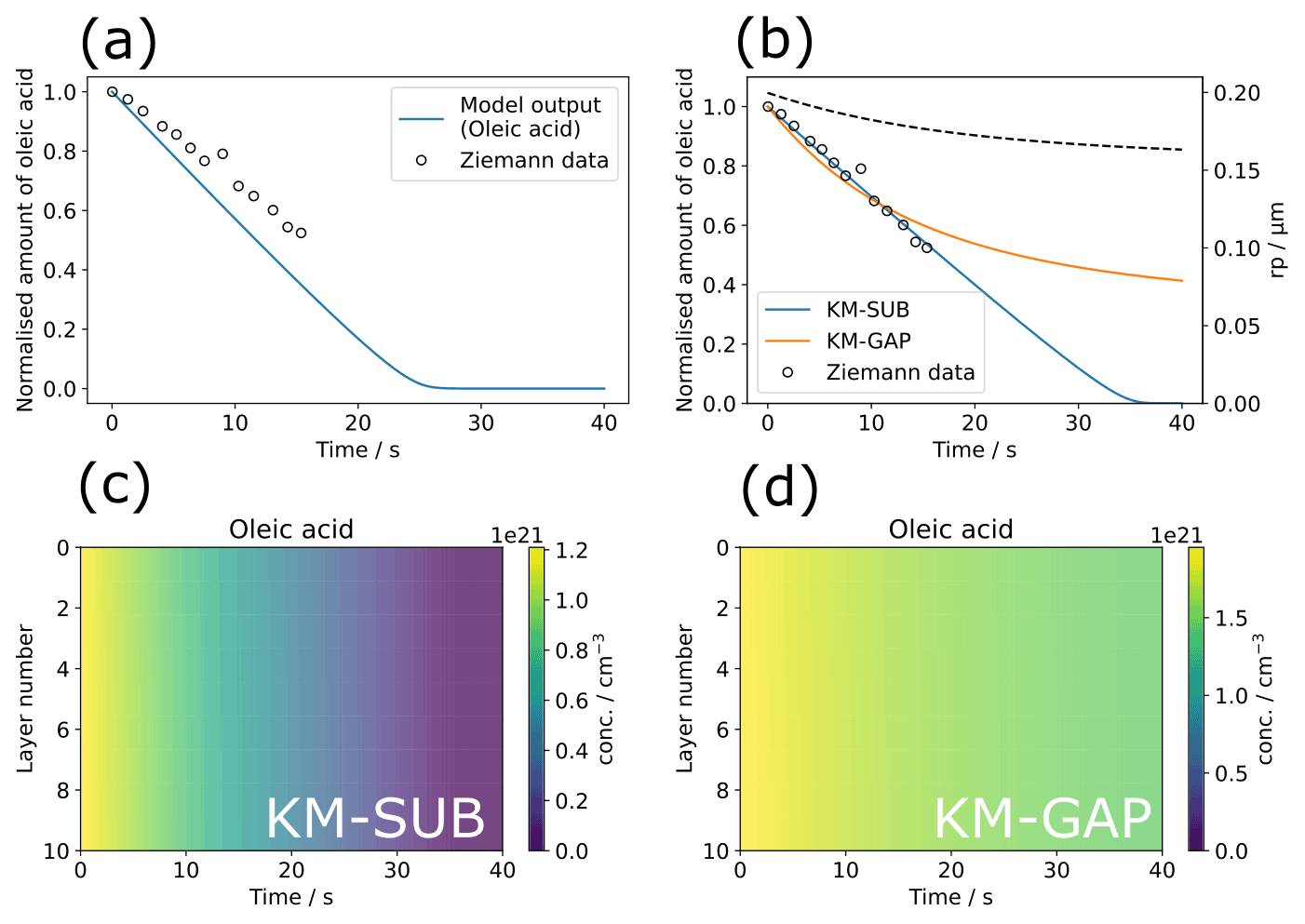
Figure 3 Model optimisation to experimental data from Ziemann (Ziemann, 2005) using the MultilayerPy model building and optimisation tool. (a) The initial model output before optimisation. (b) KM-SUB model output optimised by varying ${\mathit{\alpha }}_{\mathrm{s},\mathrm{0},\text{ozone}}$; KM-GAP model output optimised by varying ${\mathit{\alpha }}_{\mathrm{s},\mathrm{0},\text{ozone}}$ and the desorption lifetime of the ozonolysis product nonanal (τ_d,nonanal). The radius of the particle (r_p) from the KM-GAP output is also plotted as a dotted line (r_p does not change in the KM-SUB model since particle size changes are not described). (c) Depth-resolved oleic-acid concentration profile for the optimised KM-SUB model. (d) Depth-resolved oleic-acid concentration profile for the optimised KM-GAP model.

4 Case studies: oleic-acid ozonolysis

The oleic-acid–ozone reaction system is a well-established model compound for heterogeneous reactions of organic aerosols due to its prevalence as a cooking emission tracer (Lyu et al., 2021; Vicente et al., 2021; Wang et al., 2020) and has been the subject of numerous experimental studies (Dennis-Smither et al., 2012; González-Labrada et al., 2007; Hearn and Smith, 2004; Hosny et al., 2013; Hung et al., 2005; King et al., 2004, 2020; Knopf et al., 2005; Milsom et al., 2021b, a; Pfrang et al., 2017; Sebastiani et al., 2018; Smith et al., 2002; Woden et al., 2021; Zahardis and Petrucci, 2007). For this reason, it has been a popular system to model (Berkemeier et al., 2021; Gallimore et al., 2017; Milsom et al., 2022b; Pfrang et al., 2010, 2011; Shiraiwa et al., 2010, 2012). The precise reaction scheme is still not constrained, especially when considering the impact of reactive intermediates, although recent work has advanced our understanding of this system and highlighted experimental gaps to be filled (Berkemeier et al., 2021). Here, we use the oleic-acid–ozone system as a case study. Case study 1 demonstrates fitting a KM-SUB and KM-GAP model to the same oleic-acid particle ozonolysis dataset. Case study 2 demonstrates an application to an insoluble oleic-acid monolayer and the MCMC sampling procedure employed in MultilayerPy in order to estimate the uncertainty associated with a model parameter.

4.1 Case study 1: fitting KM-SUB and KM-GAP to oleic-acid particle ozonolysis data

In this case study, KM-SUB and KM-GAP models are fitted experimental data for the ozonolysis of oleic-acid particles from Ziemann (2005). This is the same example case study used in the kinetic double-layer model (K2-SUB) (Pfrang et al., 2010), KM-SUB (Shiraiwa et al., 2010) and KM-GAP (Shiraiwa et al., 2012) papers.

The radius of the particles was 0.2 µm and the gas phase ozone concentration was 7.0 × 10¹³ cm⁻³ (2.8 ppm at 101 325 Pa). In total, 10 bulk layers were initiated in our case study. A table with all other optimised parameters along with bounds for varied parameters is presented in Table S1 in the Supplement.

A modelling experiment was carried out using MultilayerPy with the data from Ziemann (Ziemann, 2005) (Fig. 3). The code used to generate these outputs is available in “crash course” and “KM-GAP model creation” Jupyter notebooks within the source code, which also describe each step of the model building process.

The differential evolution algorithm was used as the global optimiser for the KM-SUB and KM-GAP model runs in this case study (Storn and Price, 1997). The surface accommodation coefficient of ozone on a free surface (${\mathit{\alpha }}_{\mathrm{s},\mathrm{0},\text{ozone}}$) was varied in the KM-SUB model. Figure 3b demonstrates good fits to the experimental data, especially using the KM-SUB model. The parameters for the fitted KM-SUB model presented here are identical to those used to fit to the same dataset in the KM-SUB model description paper (Shiraiwa et al., 2010).

Nonanal was assumed to be volatile in the KM-GAP reaction scheme as it is the only product known to be volatile (Vesna et al., 2009). The desorption lifetimes of nonanal (τ_d,nonanal) and ${\mathit{\alpha }}_{\mathrm{s},\mathrm{0},\text{ozone}}$ were varied in this case study. As KM-GAP resolves changes in particle size via the loss or gain of volatile species to the particle, τ_d,nonanal will have an impact on the size of the particle during the model run. Time-resolved particle size information is not known for this experiment. This will affect the number concentration of oleic acid in the particle in the KM-GAP model, which considers nonanal evaporation and resulting particle size change, accounting for the significant differences seen between the KM-SUB and KM-GAP outputs, especially at times greater than the last experimental data point (∼ 17 min).

In both KM-SUB and KM-GAP models presented here the bulk phase is well-mixed, demonstrated by the lack of oleic-acid concentration gradient occurring throughout the particle during ozonolysis (Fig. 3c and d). The concentration of oleic acid in each model layer is generally higher in the KM-GAP output compared with KM-SUB due to the shrinking of the model layers accounted for in KM-GAP and caused by the removal of nonanal from the particle.

4.2 Case study 2: fitting a KM-SUB model to oleic-acid monolayer ozonolysis data, including MCMC sampling

Woden et al. (2021) ozonised insoluble floating monolayers of oleic acid deposited on water (Woden et al., 2021). The reaction kinetics were followed using neutron reflectometry (NR) and fitted parameters from an interfacial model applied to the NR data – a common method of extracting kinetic information from NR experiments (King et al., 2009, 2020; Pfrang et al., 2014; Sebastiani et al., 2018; Woden et al., 2018, 2021). The ozone concentration for the example model–data system was 323 ± 29 ppb. The construction of this case study is presented in the “insoluble monolayers” Jupyter notebook and the MCMC sampling for this case study is presented in the “MCMC sampling” Jupyter notebook.

The dissolution of oleic acid and products into the aqueous phase was turned off in the model building process by setting bulk diffusion parameters to 0. The model in this case was particularly sensitive to ${\mathit{\alpha }}_{\mathrm{s},\mathrm{0},\text{ozone}}$. This was selected as the fitting parameter.

${\mathit{\alpha }}_{\mathrm{s},\mathrm{0},\text{ozone}}$ can range between 0–1. This was set as the fitting bound for both the differential evolution (global) optimisation algorithm and the MCMC sampling procedure.

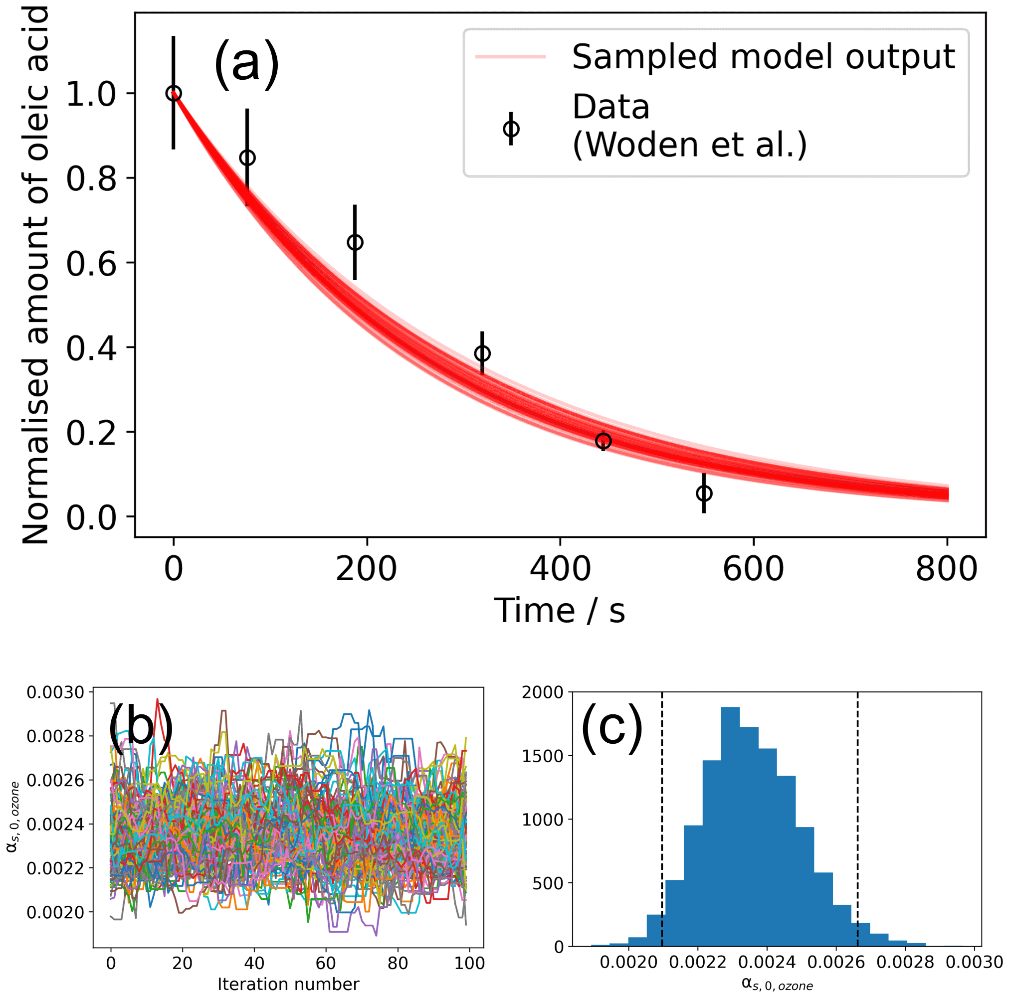
Figure 4 Result of the global optimisation MCMC sampling procedure. (a) Total of 200 model outputs sampled from the MCMC sampling procedure, showing the range of model outputs consistent with the data. (b) A plot of ${\mathit{\alpha }}_{\mathrm{s},\mathrm{0},\text{ozone}}$ vs. iteration number of the MCMC algorithm for a converged set of walkers (Markov chains). In total, 100 samples were discarded (burn-in step) before chains converged. (c) The histogram of ${\mathit{\alpha }}_{\mathrm{s},\mathrm{0},\text{ozone}}$ values derived from the walkers presented in panel (b). Vertical dashed lines represent the interval in which 95 % of the data lie.

An initial differential evolution procedure was carried out on this model–data system. This optimised value of ${\mathit{\alpha }}_{\mathrm{s},\mathrm{0},\text{ozone}}$ was then used to initialise the ensemble of walkers for the MCMC sampling procedure – this is handled by MultilayerPy. The MCMC algorithm can then be run in series or in parallel. The result of this MCMC sampling procedure is presented in Fig. 4.

The mean value of ${\mathit{\alpha }}_{\mathrm{s},\mathrm{0},\text{ozone}}$ obtained from MCMC sampling is (2.35 ± 0.14) × 10⁻³. In this case, the distribution of ${\mathit{\alpha }}_{\mathrm{s},\mathrm{0},\text{ozone}}$ is Gaussian (Fig. 4c). For other distributions, quoting an interquartile range may be more representative. The lower and upper bound for each optimised parameter is included when the user exports their modelling results. In this case, the lower and upper bounds of the interquartile range for ${\mathit{\alpha }}_{\mathrm{s},\mathrm{0},\text{ozone}}$ are 2.36 × 10⁻³ and 2.44 × 10⁻³, respectively.

Constraining model input parameters experimentally remains the best way to improve the estimation of unknown model parameters. For example, simultaneously varying the desorption lifetime of ozone (τ_d,ozone), the surface reaction rate coefficient (k_surf) and ${\mathit{\alpha }}_{\mathrm{s},\mathrm{0},\text{ozone}}$ returns a range of possible combinations of these three parameters – all of which are associated with surface processes. This is demonstrated by the strong correlation observed between these parameters during MCMC sampling (Fig. S1 in the Supplement). MultilayerPy could be used to identify which experimental parameters should be constrained and inform experimental work.

4.3 Case study 3: visualising concentration gradients and custom parameterisation

A key feature of kinetic multi-layer modelling is its ability to visualise concentration gradients in particles and films. This case study demonstrates how this is achieved using MultilayerPy by reproducing the concentration gradient modelled in a film of a semi-solid (self-organised lamellar) form of oleic acid exposed to ozone (Milsom et al., 2022b). The experimental and modelling conditions are outlined in Milsom et al. (2022b) and the corresponding “lamellar phase oleic acid” Jupyter notebook, which reproduces Fig. 5.

In this model, condensed-phase molecular diffusivity is affected by the formation of high molecular-weight oligomers. This was implemented using the diffusion regime object pictured in Fig. 2 using a Vignes-type parameterisation of molecular diffusivity, where molecular diffusion depends on the proportion of oligomer in the particle (Milsom et al., 2022b; Vignes, 1966).

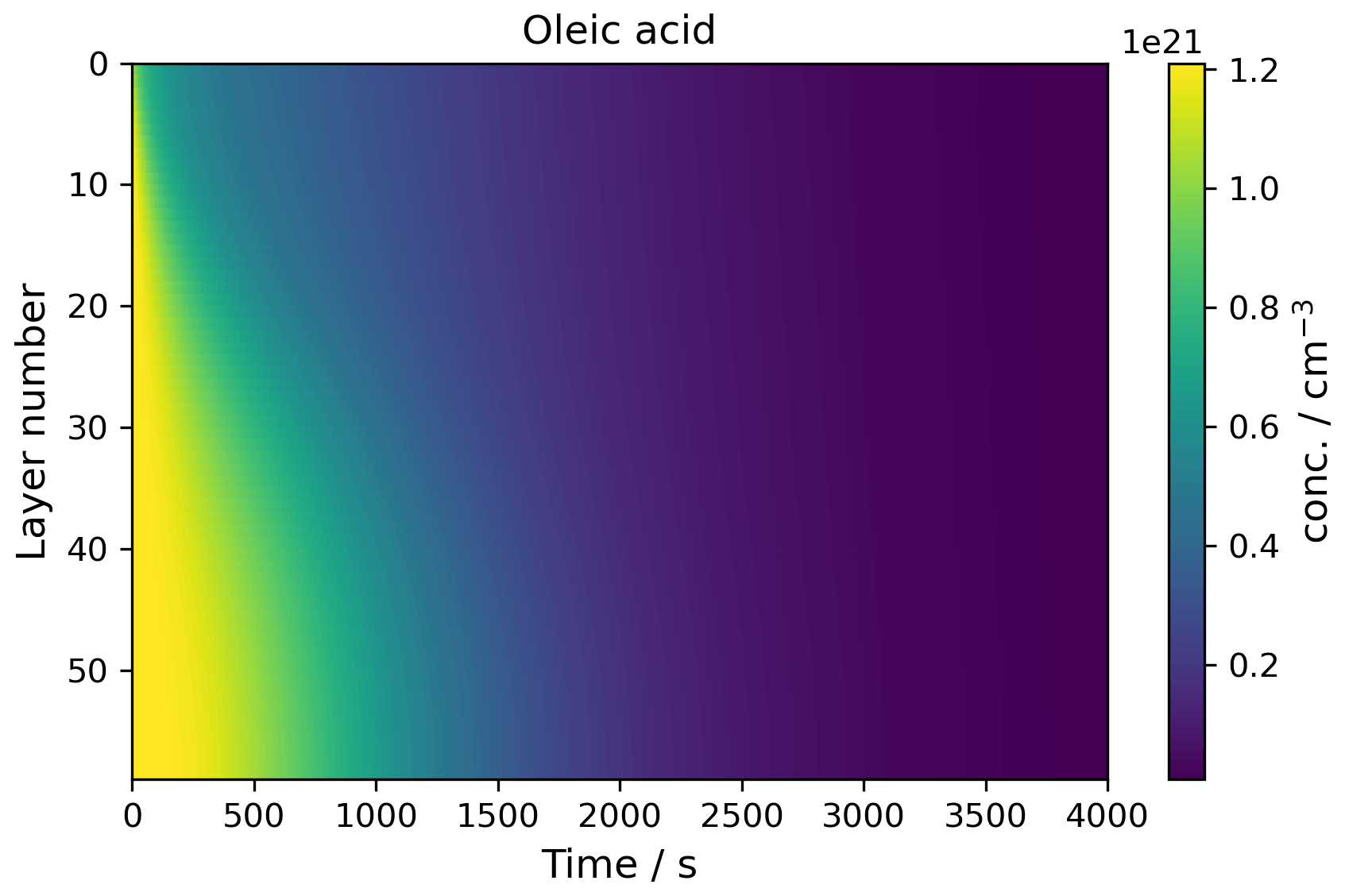
Figure 5 The concentration profile of a film of semi-solid (self-organised lamellar) oleic acid during ozonolysis. The film is 0.98 µm thick, and 77 ppm ozone was applied to the model.

The diffusivity of the dimer and trimer oligomers were related to each other via Eq. (3).

$$\begin{array}{}\text{(3)}& D_{\text{tri}}=D_{\text{di}}{\left({\displaystyle \frac{M_{\text{di}}}{M_{\text{tri}}}}\right)}^{f_{\text{diff}}},\end{array}$$

where D_di and D_tri are the diffusion coefficients of the dimer and trimer products, respectively; M_di and M_tri are the molecular masses of the dimer and trimer products, respectively; and f_diff is a scaling factor used as a fitting parameter in the model optimisation (Hosny et al., 2016; Milsom et al., 2022b).

This custom parameterisation of oligomer diffusivity is possible in MultilayerPy via a parameter evolution function that the user can supply, a tutorial for which is found in the “parameter evolution” Jupyter notebook in the source code along with this specific example in the “lamellar phase oleic acid” Jupyter notebook. The parameter evolution function could be used to introduce changes in experimental conditions during the model simulation (e.g. slowly increasing the concentration of a reactive gas or introducing a temperature profile, making certain parameters temperature dependent). There is sufficient flexibility in the MultilayerPy framework for the user to incorporate more complex model parameterisations.

5 Conclusions: summary and future developments

This open-source model construction framework represents a first step towards more reproducible kinetic multi-layer modelling of atmospheric aerosols and films. The way that models are constructed and the ease with which model code can be generated in MultilayerPy encourage the user to share their models with the community.

MultilayerPy provides a simple model construction and optimisation pipeline for the user to follow with a few lines of code needed to produce results. This is a major practical advance compared to manually typing out ODEs – which can be an unnecessary source of error and is time consuming. There is sufficient flexibility to suit more complex systems with parameterisation of model input parameters, along with customisation of the source model code “under the hood”.

The trade-off when integrating systems of ODEs written in a high-level programming language such as Python or MATLAB is that, compared with C/C$++$ and FORTRAN, these integrations are relatively slow. Future work will consider ways of speeding up ODE integration. This is partially addressed via the ability to parallelise the global optimisation and MCMC algorithms. The Julia programming language is also an attractive proposition, allowing human-readable code to be written and run at speeds faster than that of Python and MATLAB. Indeed, Julia has recently been applied in an atmospheric context to construct box models (Huang and Topping, 2021). These are feasible options for the direction of MultilayerPy development in the future.

The modular way in which MultilayerPy is constructed makes future modular developments relatively straightforward. Other modelling systems based on the kinetic multi-layer model presented here (KM-SUB and KM-GAP) have been developed and include other “compartments” such as the skin (KM-SUB-skin) (Lakey et al., 2017), indoor air boundary layer (KM-BL) (Morrison et al., 2019), film formation and growth (KM-FILM) (Lakey et al., 2021), and epithelial lining fluid (KM-SUB-ELF) (Lelieveld et al., 2021). Future iterations of MultilayerPy could incorporate such multi-compartment models, coupling different processes occurring in various environments and contexts.

As an open-source project, contributions from the particle and film modelling community are strongly encouraged and will help push the project forward and achieve collective goals. This will also facilitate scientific collaboration and encourage more reproducible modelling studies as a result.

Appendix A

Table of variable names, descriptions and units supplied to models created in MultilayerPy. The unit of length in these models is cm and the units for surface and bulk concentrations of model components are cm⁻² and cm⁻³, respectively.

Parameter name	Description (units)
delta_1	Molecular diameter of component 1 (cm)
w_1	Mean thermal velocity of component 1 in the gas phase (cm s−1)
H_1	Henry's law coefficient ($\mathrm{mol}{\mathrm{cm}}^{-\mathrm{3}}{\mathrm{atm}}^{-\mathrm{1}}$)
alpha_s_0_1	Surface accommodation coefficient of component 1 on a clear surface
Db_1	Bulk diffusion coefficient of component 1 (cm2 s−1)
Db_1_2	Bulk diffusion coefficient of component 1 in component 2 (cm2 s−1)
T	Temperature (K)
k_1_2	Second-order rate coefficient for the bulk reaction of component 1 and component 2 (cm3 s−1)
k_1_2_surf	Second-order rate coefficient for the surface reaction of component 1 and component 2 (cm2 s−1)
k1_1	First-order decay constant for component 1 (s−1)
Xgs_1	Near-surface gas phase concentration of component 1 (cm−3)
Zgs_1	Near-surface gas phase concentration of component 1 with KM-GAP notation (cm−3)
p_1	Equilibrium vapour pressure of component 1 (Pa)
Td_1	Desorption lifetime of component 1 (s)
scale_bulk_to_surf	Scaling factor applied to bulk reaction rate coefficient to return the surface reaction
	rate coefficient (cm)

Appendix B: Basic package installation instructions

This package was developed using the standard Anaconda Python distribution, and this distribution is recommended for the novice user. For basic “plug and play” use, the Zenodo repository can be downloaded and extracted (see the “Code availability” section). This places the source code in the extraction directory, and any work with the package must be carried out in that directory because the package has not been installed in the Python environment. This is the best way for the user to get started quickly and learn how to use the package.

To install the package in the user's Python environment, a “pip install multilayerpy” command in the Anaconda terminal window is required. This will install the latest built distribution of MultilayerPy, which is stored on the Python Package Index (PyPI). After this method of installation, the user can use MultilayerPy anywhere on their system and is not limited to a particular working directory.

Full installation instructions and package dependencies are listed and updated on the project repository (see the “Code availability” section).

It is recommended that a new user starts by working through the “MultilayerPy crash course” tutorial notebook to learn how the package works. This notebook can also be a template for the user's own projects.