Inland lake temperature initialization via coupled cycling with atmospheric data assimilation

Application of lake models coupled within earth-system prediction models, especially for predictions from days to weeks, requires accurate initialization of lake temperatures. Commonly used methods to initialize lake temperatures include interpolation of global sea-surface temperature (SST) analyses to inland lakes, daily satellite-based observations, or model-based reanalyses. However, each of these methods have limitations in capturing the temporal characteristics of lake temperatures (e.g., effects of anomalously warm or cold weather) for all lakes within a geographic region and/or during extended cloudy periods. An alternative lake-initialization method was developed which uses two-way-coupled cycling of a small-lake model within an hourly data assimilation system of a weather prediction model. The lake model simulated lake temperatures were compared with other estimates from satellite and in situ observations and interpolated-SST data for a multi-month period in 2021. The lake cycling initialization, now applied to two operational US NOAA weather models, was found to decrease errors in lake surface temperature from as much as 5–10 K vs. interpolated-SST data to about 1–2 K compared to available in situ and satellite observations.

1 Introduction

Inclusion of lake representation into numerical weather prediction (NWP) models has become increasingly necessary to further improve representation of atmosphere–surface fluxes of heat and moisture as model grid resolution becomes finer. Representation of lake physics to provide time-varying lake surface properties (e.g., Subin et al., 2012) is essential to improve fluxes of heat, moisture, and momentum between the surface and atmosphere (Hostetler et al., 1993; Thiery et al., 2014). Lake representation is part of the overall surface treatment including land-surface models (LSMs) necessary to accurately model the evolution of the planetary boundary layer in the atmosphere. Lakes are estimated to cover 3.7 % of the global non-glaciated land area (Verpoorter et al., 2014), and they significantly moderate sensible heat and moisture fluxes from this “land” (i.e., non-ocean) area. Water impoundments (reservoirs) that used to account for about 6 % of these “lake” areas (Downing et al., 2006) have recently increased to 9 % (Vanderkelen et al., 2021). Initial conditions for both land and lake surface are an important consideration due to far larger thermal inertia for soil or water than for air. Consequently, incorrect soil or lake initial conditions can result in erroneous heat and moisture fluxes that may persist for days and even weeks (e.g., Dirmeyer et al., 2018). This potential source of error in fluxes is more pronounced for lake areas with far larger thermal inertia and heat storage than even saturated soils.

In operational US NOAA weather prediction models (global and regional) up to this point, daily sea-surface temperature (SST) analyses have been used to specify the surface water temperatures for even small inland lakes. Inland lake temperatures in North America have been obtained by the interpolation of SST values from the ocean and the Laurentian Great Lakes. An alternative is to incorporate one-dimensional (1-D) lake models within NWP models and use a continuous lake simulation forced by atmospheric conditions updated regularly by new atmospheric observations to obtain realistic lake water temperatures (e.g., “cycling”). This cycling to initialize small lakes in NOAA operational regional weather prediction models complements loose coupling with a 3-D hydrodynamical lake model for the Laurentian Great Lakes as described elsewhere in Fujisaki-Manome et al. (2020).

Lake representation (via one-dimensional – 1-D – models, as in LSMs) within NWP models is beneficial by providing a first-order accurate lagged effect of the seasonal variation in temperature, with lake water remaining colder than nearby land in spring and warmer in autumn. The outcomes are desirable, as described by Balsamo et al. (2012), for instance by accurately representing increased evaporative fluxes in the fall. Thus, use of a 1-D lake model has the potential to improve over land representation by capturing this slower seasonal response.

However, lake temperature initialization from SST (e.g., Mallard et al., 2015) can exaggerate this seasonal slower response. Shallow lakes warm more slowly in spring than surrounding land but more quickly than nearby deeper lakes. Even in summer, it will take at least 1–2 weeks for cycled 1-D models to adjust from values interpolated from deeper-lake temperatures to become more realistic for shallow lakes. Therefore, lake temperature initialization becomes the most important factor to accurately simulate sensible and latent heat fluxes from lakes for short- to medium-range NWP – more so than the use of the lake model itself. One option to solve the lake-initialization problem is to use a model-based climatology for seasonal variation of lake temperatures (Balsamo et al., 2012; Balsamo, 2013, ECMWF) using a 1-D lake model forced by reanalysis data. The 1-D lake model used by ECMWF for this method is the two-layer FLake (Freshwater Lake Model) model (Mironov et al., 2010; Balsamo et al., 2012; Boussetta et al., 2021) and also implemented into their Integrated Forecast System (IFS) in 2015. A similar technique was applied by Mironov et al. (2010) using FLake for the COSMO model. Kourzeneva et al. (2012a) describe application of 20-year reanalysis data to create a global lake climatology dataset using FLake. This technique avoids a new spin-up with each new run but cannot capture unique weather regime variations in a given region and time. The UK Met Office uses satellite data to update their lake surface water temperatures using the previous day values as a background (Fiedler et al., 2014). Another option to solve the lake-initialization problem, described here, is lake temperature evolution, referred to as “lake cycling”, with the ongoing 1-D lake prediction within an NWP model, a cost-free option if the atmospheric conditions are relatively accurate.

Data assimilation for land-surface fields (e.g., soil temperature, soil moisture, snow cover, snow water equivalent, snow temperature) has been very beneficial for improved short-range weather prediction accuracy (e.g., Balsamo and Mahfouf, 2020; Muñoz-Sabater et al., 2019; Benjamin et al., 2022, others), but lake temperature has not been a part of this surface data assimilation. In December 2020, the two NOAA hourly updated weather models, the 13 km Rapid Refresh (RAP) and 3 km High-Resolution Rapid Refresh (HRRR), implemented an interactive small-lake multi-layer 1-D lake model, the first NOAA weather models to do so. The lake coverage for the HRRR model is shown in Fig. 1 (RAP model lake coverage not shown). The HRRR and RAP weather models are coupled with the 10-layer Community Land Model (CLM) version 4.5 lake model (Subin et al., 2012; Mallard et al., 2015), an option within the community Weather Research and Forecast Model (WRF, Skamarock et al., 2019). The CLM lake model is a 1-D thermal diffusion model allowing two-way coupling with the atmosphere. Virtually no additional computational cost (<0.1 %) was added by use of the CLM lake model within the HRRR model. To initialize small-lake temperatures in the RAP and HRRR, all lake variables have been evolving (e.g., lake cycling) since summer 2018 depending on the cycled atmospheric conditions and the lake model physics as discussed in Sect. 4. This cycling is similar to the land-surface cycling in HRRR and RAP as described by Benjamin et al. (2022). The 1-D lake model cannot represent 3-D hydrodynamical processes in larger bodies of water. Thus, a second major improvement in 2020 with lake representation in the NOAA 3 km HRRR model occurred with the implementation of lagged data coupling with the 3-D hydrodynamic-ice model for the much larger Laurentian Great Lakes as described by Fujisaki-Manome et al. (2020). These new improved lake treatments are in the newer HRRR version 4 (HRRRv4) replacing the previous HRRRv3 (differences described in Dowell et al., 2022; hereafter D22).

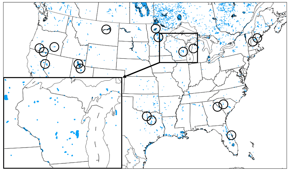
Figure 1 Small-lake areas for the 3 km HRRR domain using the MODIS 15 arcsec resolution data for land/water and lake information. Only small-lake areas treated in HRRR by the 1-D CLM lake model are shown. A zoomed-in insert for HRRR small-lake coverage in the vicinity of the state of Wisconsin is shown in the lower left. Out of the 1 900 000 grid points in this HRRR CONUS domain, 12 305 of them (∼0.6 %) are for small lakes (excluding the five Laurentian Great Lakes treated by separate coupling as described in the text). Lakes circled in black were related to problem reports from US National Weather Service Forecast Offices on nearby deficient 2 m air temperature or dew point forecasts in NOAA hourly updated models as discussed in Sect. 2.

Here, we describe the design and results of a unique approach to inland-small-lake initialization by cycling with hourly updating of atmospheric conditions (clouds/radiation, near-surface temperature/moisture/winds). This lake initialization via cycling is an important component of earth-system coupled modeling for effective NWP, with goals to improve prediction of 2 m (air) temperature and moisture, cloud, boundary-layer conditions, and precipitation for situational awareness enabling short-range decision making (e.g., aviation, severe weather, hydrology, energy).

2 The lake-initialization problem

For the NOAA hourly updated mesoscale models, used frequently for short-range weather prediction, poor 2 m air temperature and/or dew point forecasts have been reported intermittently during 2004–2019 by the US National Weather Service (NWS) in the vicinity of inland lakes (Fig. 1). These hourly updated models included the Rapid Update Cycle (RUC, Benjamin et al., 2004) with horizontal grid spacing decreasing from 40 to 20 to 13 km (Benjamin et al., 2010), succeeded by the 13 km RAP and 3 km HRRR (Benjamin et al., 2016; D22, James et al., 2022 – J22). Many of these reported systematic deficiencies from the US NWS were for the 2.5 km NOAA Real-Time Mesoscale Analysis (RTMA, De Pondeca et al., 2011), using 1 h forecasts from the 3 km HRRR as a background. The most common report was too-low 2 m air temperatures near inland lakes in late spring and summer. At times, spurious prediction of fog formation was also noted on or near small lakes due to too-cold lake temperatures and erroneous heat and moisture fluxes into the atmosphere.

Further investigation revealed the water temperatures for small lakes used in NOAA weather models were assigned via horizontal interpolation from larger, deeper bodies of water (with available AVHRR data) in the design for the NOAA real-time gridded SST analysis (RTG_SST_HR, Gemmill et al., 2007). An example of the analysis is shown in Fig. 2. Temperature for the larger, deeper-water areas has a lesser and more lagged seasonal variation than the smaller, shallower lake areas due to their large heat storage capacity. Therefore, use of the NOAA SST fields for lake temperatures resulted in generally too-low values through spring and summer and even into autumn. In situations with atmospheric cold outbreaks in the autumn, shallow lake temperatures quickly decrease (as reflected with lake cycling), and SST-based estimated lake temperatures were too high. This behavior was consistent with the HRRR and RTMA deficiencies noted by forecasters. In February 2020, NOAA changed from the RTG_SST_HR to a near-surface sea temperature (NSST; see NWS, 2020) for SSTs, but using the same horizontal interpolation method to estimate small-lake temperatures resulting in the same temperature biases for small lakes.

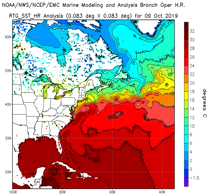
Figure 2 An example of small-lake temperatures spatially interpolated from deeper-water temperature data in the NOAA SST analysis (Gemmill et al., 2007). For 9 October 2019, provided by NOAA National Weather Service.

Hamill (2020), in a comparison benchmarking a statistical method for 2 m temperature (at 00:00 UTC), showed the same problem with large summer temperature biases from the HRRRv3 1 h forecasts in August 2018 especially in the vicinity of lakes (his Figs. 10 and 11). His results are shown in Fig. 3, with three stations showing coldest biases (at 00:00 UTC) greater than 2 K (circled in red), all adjacent to lakes. In Fig. 3, these circled stations, from north to south, are KFGN (Flag Island on Lake of the Woods; >3 K cold bias), KRRT – Warroad, MN (west of Lake of the Woods), and KVWU – Waskish, MN (east of Red Lake). The overall warm or cold biases are generally <2 K, but these stations adjacent to lakes are outliers, consistent with introduction of cold-biased lake temperatures through the NSST.

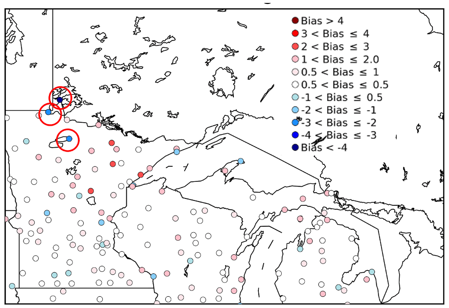
Figure 3 The 2 m temperature biases for 1 h HRRR forecasts valid at 00:00 UTC in August 2018 (from HRRRv3, before introduction of lake cycling and using NSST estimates instead; HRRR versions and dates are listed in D22). Stations with low bias less than −2 K are circled in red. (Credit and thanks to Thomas Hamill for providing a regional version of his Fig. 10b in Hamill, 2020.)

With its 3 km grid spacing, the HRRR model can resolve many inland lakes (Fig. 1). Specification of surface temperatures for these small lakes using the horizontal interpolation from the NOAA SST fields was problematic, being determined by interpolation from large-lake and ocean temperatures.

In summary, errors in specified lake temperatures (as well as ice cover and concentration) due to spatial interpolation from oceans and larger lakes can lead to degraded atmospheric predictions in the vicinity of lakes. For small lakes, poor short-range 2 m temperature (T) and 2 m dew point temperature (T_d) forecasts were noted in the vicinity of lakes, especially from spring through summer and into autumn. Specifically, fluxes from lakes were often poorly estimated due to inaccurate lake temperature fields.

3 Lake model for coupling with NOAA regional atmospheric models

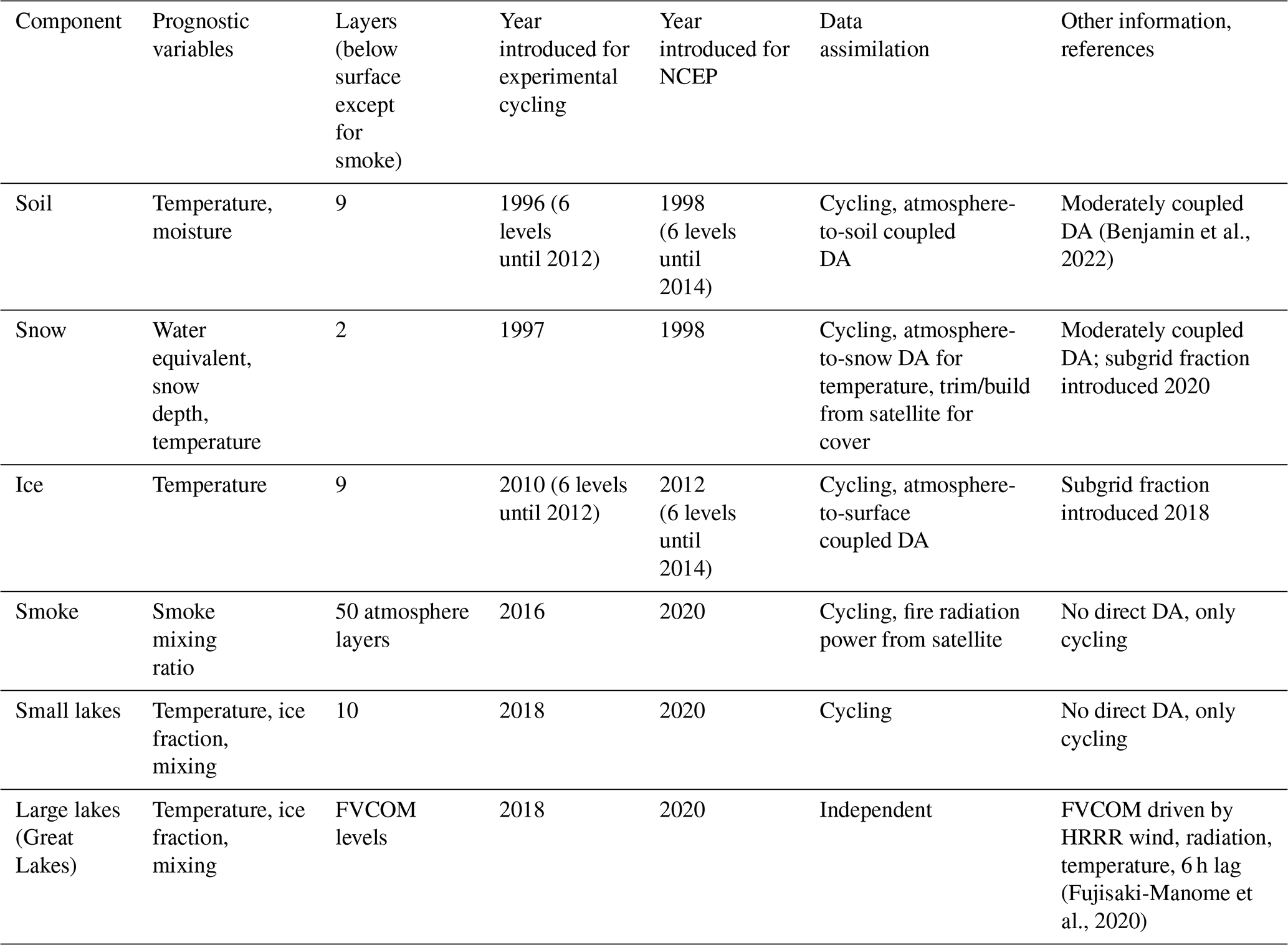
To complement the now-commonplace (in NWP models) coupling with land-surface models (LSMs) to improve fluxes into the atmosphere, a multi-level 1-D lake model was implemented within the operational 3 km HRRRv4 and 13 km RAP weather models in December 2020, an extension to atmosphere–surface coupling. An effective lake initialization is a necessary complement for the lake model coupling, as described in Sect. 4. Different earth–system coupling processes represented in the HRRR and RAP models are described in Table 1, including land, snow, ice, and smoke. The Community Land Model (CLM) lake model (same in versions 4.5 and 5.0) was added for smaller lakes as an option in the WRF model version 3.6 (Mallard et al., 2015). The CLM lake model is described in more detail below with its configuration for the NOAA HRRRv4 and RAP weather models. A detailed description of the physical processes (cloud microphysics, turbulent exchange, land surface, etc.) in the HRRR and RAP models is described by D22 and Benjamin et al. (2016). An additional improvement in lake–atmosphere coupling in NOAA weather models for large lakes (>15 000 km²) was recently introduced – a coupling between the NOAA HRRR model using predicted lake temperatures and ice concentration fields from the NOAA GLERL/NOS three-dimensional hydrodynamic-ice model run in real time over the Laurentian Great Lakes, as described by Fujisaki-Manome et al. (2020). This hydrodynamic-ice model is based on the Finite Volume Community Ocean Model (FVCOM, Chen et al., 2006, 2013) coupled with the unstructured grid version of Los Alamos sea ice model (CICE; Gao et al., 2011) and is applied to the NOAA Great Lakes Operational Forecast System (GLOFS, Anderson et al., 2018). This time-lagged data coupling (alternate applications of HRRR atmospheric forcing and FVCOM–CICE lake forcing about 6–12 h in advance) was incorporated to improve lake-effect snow (LES) predictions in winter but has also been found to improve near-lake atmospheric predictions year-round especially for upwelling events in the warm season. The use of FVCOM–CICE to specify lake temperatures addresses previous errors in SST from relatively fast changes in lake temperatures due to cold air outbreaks or upwelling events. These changes sometimes escape AVHRR-derived SST detection due to multi-day cloud obscuration.

Table 1 Earth-system coupling added to NOAA regional models (HRRR, RAP, RUC – pre-2012).

3.1 CLM lake model applied to HRRR for smaller inland lakes

Subin et al. (2012) describe the 1-D CLM lake model as applied within the Community Earth System Model (CESM) as a component of the overall CESM CLM (Lawrence et al., 2019). Gu et al. (2015) describe the introduction of the CLM lake model into the WRF model and initial experiments using its 1-D solution for both Lake Superior (average depth of 147 m) and Lake Erie (average depth of 19 m). The CLM lake model divides the vertical lake profile into 10 layers driven by wind-driven eddies. The atmospheric inputs into the model are temperature, water vapor, horizontal wind components from the lowest atmospheric level, and shortwave and longwave radiative fluxes (from the HRRR model in this application). The CLM lake model then provides latent heat and sensible heat fluxes back to the HRRR. The CLM lake model is called every 20 s within the HRRR model. The CLM lake model was configured with the top layer fixed to a 10 cm thickness (Gu et al., 2015) and with the rest of the lake depth divided evenly into the other nine layers. Energy transfer (heat and kinetic energy) occurs between lake layers via eddy and molecular diffusion as a function of the vertical temperature gradient. The version of the CLM lake model used for HRRRv4 and RAP was introduced with CLM version 4.5 and continues without change in CLM version 5 (Lawrence et al., 2019). The CLM lake model also uses a 10-layer soil model beneath the lake, a multi-layer ice formation model and an up-to-5-layer snow-on-ice model (Gu et al., 2015). Again, testing of the CLM lake model by the authors within WRF showed computational efficiency of the model with no change of even 0.1 % in run time with the HRRR and RAP applications. Multiple layers in lake models better represent vertical mixing processes in the lake. By intention, the CLM lake model was only applied for the HRRR and RAP model to smaller lakes, since NOAA began at the same time to provide temperature and ice cover through GLOFS for the Laurentian Great Lakes through the 3-D hydrodynamic-ice model (Fujisaki-Manome et al., 2020; Anderson et al., 2018).

3.2 Lake area mask

Grid points were assigned as lake points when the fraction of lake coverage in the grid cell (derived from yet finer 15 arcsec MODIS data) exceeds 50 % and when HRRR grid point elevation is more than 5 m a.s.l. (above sea level, to distinguish from ocean) and is disconnected from ocean areas with the 3 km land–water mask. The lake water mask is therefore binary, set to either 1 or 0. This binary approach at 3 km seemed capable of capturing the effect of lakes on regional heat and moisture fluxes. The alternative subgrid lake fraction approach was used by ECMWF with their 9 km model (Choulga et al., 2019).

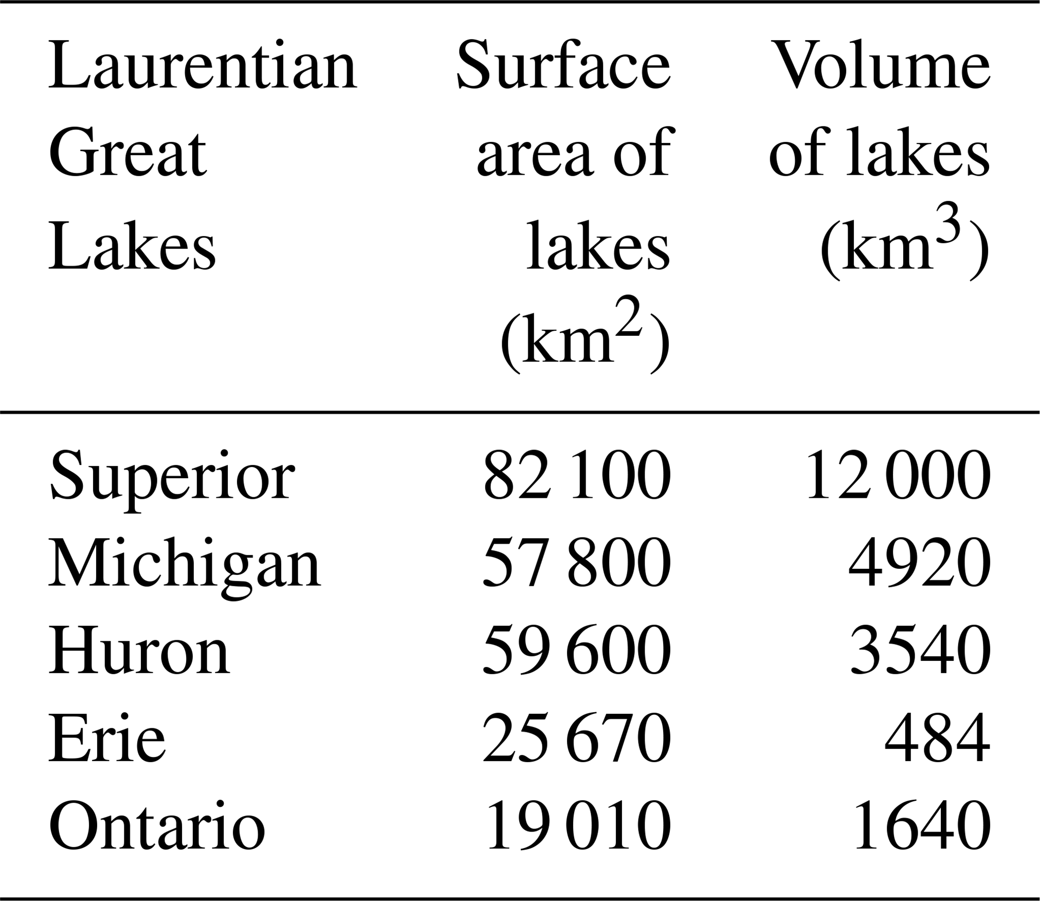
An overview of the lake number, areal coverage, and integrated volume for the 3 km HRRRv4 model are depicted in Table 2. The HRRR CONUS domain (Fig. 1) is able to represent 1864 separate lakes occupying 0.6 % of the entire domain. These water bodies represented in HRRR as “lakes” include reservoirs and larger rivers, and about half of the 1864 lakes are single-grid-point lakes. The 16 largest lakes in the HRRR CONUS domain have surface area greater than 1000 km², 9 in Canada and 2 on the US–Canada border (Lake of the Woods and Lake St. Clair). In contrast, the five Laurentian Great Lakes (Table 3) range in size from 82 000 km² (Superior) to 19 000 km² (Ontario), and, therefore, their representation in the coupled HRRR system (Table 1) is handled with 3-D hydrodynamic-ice models (Fujisaki-Manome et al., 2020).

Table 2 Characteristics of small lakes (not including the five Laurentian Great Lakes) resolved in the 3 km HRRRv4 CONUS domain over the lower 48 United States and adjacent areas of Canada and Mexico. Grid points were assigned as having a lake land use for points with at least 50 % lake representation from the higher-resolution 15 arcsec MODIS land-use data.

Table 3 Characteristics of the five Laurentian Great Lakes (surface area, volume) (Hunter et al., 2015).

The lake area mask for the 3 km HRRRv4 used an algorithm for identifying an ocean area mask for all areas with contiguous water areas and leaving other areas also below 5 m a.s.l. as near-ocean lagoon regions treated as lakes with the CLM 1-D lake model. These lagoon areas separated from the ocean by barrier islands in the HRRR representation (Fig. 1) include the Intracoastal Waterway in Texas largely separated from the Gulf of Mexico by Padre Island, Indian River in Florida largely separated from the Atlantic Ocean by Merritt Island, and Lake Pontchartrain in Louisiana. This ocean-contiguity technique is similar to the flood-filling technique used by ECMWF (Choulga et al., 2019).

Figure 4 Lake depth for small lakes in a subset of the HRRR domain.

3.3 Lake depths

Lake depths for the HRRRv4-WRF-CLM lake configuration (Fig. 4) are assigned from a global dataset provided by Kourzeneva et al. (2012b, hereafter K12). For some smaller lakes identified using the 15 arcsec MODIS land–water mask not found in K12, a 50 m depth was assumed (too deep, will be reduced in future). K12 identified uncertainties in their own database including estimates of lake depth and errors in coastlines. More recently, ECMWF applied a 10 m depth as a default depth for these small lakes (Choulga et al., 2019). For many lakes in the K12 database, a single value for maximum lake depth had been applied to all lake points, which results in excessive lake water volume and too-cold temperatures as discussed in Sect. 5. However, the K12 database still allows overall differentiation between shallow and deep lakes.

3.4 Turbidity

A single value for turbidity to describe absorption of downward shortwave radiation is used in CLM, allowing for a moderate amount of suspended sedimentation. Subin et al. (2012) describe other options for variations in radiative transfer in lake bodies to capture degrees of eutrophication, but these are not used here.

3.5 Salinity

The CLM lake model is configured for fresh water. The authors manually modified the freezing temperature to account for non-zero salinity (Railsback, 2006) from 0 to −5 ^∘C for Mono Lake in California and Great Salt Lake (GSL) in Utah to capture the effect of salinity. Other areas of water impoundment from coastal lagoons in the 3 km HRRR lake representation (Fig. 1) also have, in reality, non-zero salinity (e.g., along the coasts of the Gulf of Mexico and the Atlantic Ocean), but this is not applied in HRRR/RAP. Moreover, no change in freezing temperature is necessary for these areas anyway.

3.6 Elevation

The elevation value (above sea level) assigned to each lake grid point is the same assigned to that from the atmospheric model, which may be different from reality but at least consistent with the atmospheric conditions. As mentioned earlier, the minimum elevation above sea level of a grid point to be assigned as a lake is 5 m; other water grid points are assumed to be ocean.

3.7 Special situations for CLM lake model application

The algorithm for the turbulent heat flux calculation in the CLM lake model was mainly based on Zeng et al. (1998), except that roughness length scales for temperature and humidity are the same as roughness length scale for momentum for its WRF lake application, while they are updated dynamically in CLM 4.5. Charusombat et al. (2018) showed that the same roughness length scales for temperature and salinity as that for momentum could result in overestimated surface sensible and latent heat fluxes in autumn and winter. Therefore, a revision to the CLMv4.5 lake model was introduced for modified roughness lengths over water using modified formulations of the Coupled Ocean-Atmosphere Response Experiment (COARE) algorithm as described by Charusombat et al. (2018) to improve surface sensible and latent heat fluxes.

For GSL with a very high value of salinity (270 ppt north of ∼41.22^∘ N with freezing point of 249 K and 150 ppt south of ∼41.22^∘ N with freezing point at 263 K), a change of freezing temperature to −5 ^∘C appeared to be not sufficient to keep the lake ice-free during the cold outbreaks in winter in this high-elevation area. GSL is unusual in various aspects – it is hypersaline (far more saline than the ocean), the largest terminal lake (without outflow) in the Western Hemisphere (Belovsky et al., 2011), shallow (mean depth of 5 m), and subject to very strong eutrophication (Belovsky et al., 2011). According to GSL climatology the lake stays ice-free all winter, and its temperature goes slightly below freezing only for a very short period in January and February. Thus, we presume that the CLM lake model needs to allow turbidity variation (see Sect. 3.4). A solution to this representation problem was use of a bi-weekly climatology over each 1-year period to bound the cycled GSL temperature at initial forecast time not to deviate more than ±3 ^∘C from the climatological value interpolated to the current day of year. Also, using special code, GSL was forced stay ice-free for the whole year as observed.

3.8 Time step

The CLM lake model within the HRRR/RAP weather models was run with the same time step as for other physical processes in the HRRR model (20 s) and the RAP model (60 s). Again, even with this relatively high frequency for calling the CLM lake model, the computational expense was extremely small – less than 0.1 % of overall HRRR run time.

4 Initialization for small-lake temperatures by cycling with ongoing atmospheric predictions – a strategy

The central strategy described in this paper is to use accurate, ongoing atmospheric forcing with a computationally inexpensive 1-D lake model to obtain an equilibrium state of a lake temperature profile. This technique responds appropriately to strong changes in atmospheric forcing (e.g., cold air outbreak or excessive heat events). With the NOAA HRRR and RAP atmospheric models performing hourly data assimilation of a broad set of hourly observations, accurate atmospheric forcing is available.

The RAP and HRRR hourly data assimilation cycles include these aspects, all of which are important for cycling initialization of inland lakes. First, cloud assimilation (from satellite and ceilometer data) is performed to ensure accurate shortwave and longwave radiation fields (Benjamin et al., 2021). Second, radar reflectivity data are assimilated as part of a 3 km ensemble data assimilation system to ensure accurate short-range precipitation (Weygandt et al., 2022; D22; J22; Benjamin et al., 2016). Finally, 2 m air temperature and moisture and 10 m wind observations are effectively assimilated (i.e., producing more accurate predictions), including representation through the boundary layer using pseudo-innovations (James and Benjamin, 2017, meaning estimated observation–background forecast differences but not actual). Other information on the HRRR/RAP data assimilation is provided by Benjamin et al. (2016) and D22.

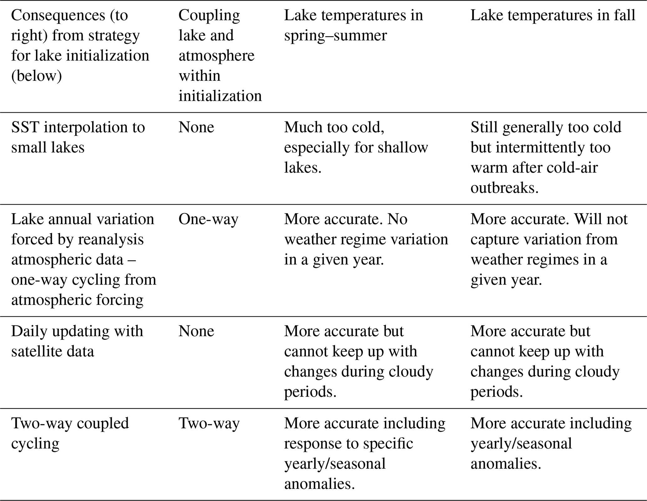
Table 4 Expected seasonal lake–atmosphere temperature consequences from different lake-initialization strategies.

The cycling of the 10-level CLM lake model within the then-experimental HRRRv4 started on 24 August 2018. After 10 d of cycling (Fig. 5), differences in lake temperatures between HRRRv4 and the operational HRRRv3 using interpolated NSST data were evident of 5–15 ^∘F (3–12 ^∘C or 276–285 K), showing that the adjustment with realistic atmospheric conditions and use of the CLM lake model with roughly accurate lake depth data was very effective.

Possible approaches for initializing lake temperatures are summarized in Table 4. The simplest option is via larger-scale water temperature data (SST data) with horizontal interpolation to smaller water areas including inland lakes and reservoirs; this was the previous strategy for the HRRRv3 and older RAP models before introduction of cycling using the CLM lake model. An alternate strategy is to run lake models over a multi-year period forced by reanalysis atmospheric data (ERA-Interim) as described by Balsamo et al. (2012), Dutra et al. (2010), and Balsamo (2013) for the ECMWF to obtain a yearly varying climatology of lake temperature for all lakes represented. This method will capture the mean annual variation of lake temperatures. However, due to multi-year averaging, it cannot represent anomalous conditions in a given year (sustained heat or sustained cold conditions), which can modify temperatures especially for shallow lakes by several kelvin within 1–2 weeks. Use of daily updating from satellite data can be effective (e.g., MetOffice – Fiedler et al., 2014) under clear-sky conditions. Full cycling of the lake model within an ongoing coupled weather model, the strategy described in this paper, can represent the lingering effects of anomalously warm or cold weather upon lake temperatures and the resultant fluxes.

The two-way-coupled cycling (Table 4) used now in the HRRR and RAP models benefits via hourly data assimilation using the latest hourly observations both for the atmosphere (D22) and land-surface snow conditions (Benjamin et al., 2021). In the 3 km HRRR model, the 3-D state of the atmosphere, land surface, and inland lake conditions are advanced on 20 s time steps using the HRRR-specific configuration (described in D22) of the WRF model (Powers et al., 2017; Mallard et al., 2015). As atmospheric conditions change every 20 s (including temperature, moisture, wind, and radiation), the exchange of heat, moisture, and momentum between inland lake points and the atmosphere also varies. Lake temperature is not modified in the hourly data assimilation step, but the ongoing exchange recalculated every 20 s forces an evolution of lake conditions to values consistent with atmospheric conditions. ECMWF applies a similar ongoing cycling for lake prognostic variables (ECMWF, 2020) for lake initialization.

Figure 5 Lake surface temperatures from 18 h forecasts valid at 15:00 UTC on 3 September 2018 for the (a) operational HRRRv3 using NSST for lake temperatures and (b) then-experimental HRRRv4 with CLM lake model and cycling.

A similar challenge is the initialization of lake ice cover. Similar to the treatment for lake temperature, cycling of a multi-level lake model (like the CLM lake model) can provide an alternative, adaptive-in-time method for lake ice initialization. NOAA has used in the HRRR and RAP the daily IMS ice cover product (https://usicecenter.gov/Products/ImsHome, last access: 26 August 2022) (US National Ice Center, 2021) for binary (non-fractional) lake ice cover. The IMS ice cover is used for oceans and large lakes (e.g., for RAP for Great Slave Lake and Great Bear Lake in northern Canada). For small lakes below the resolution of the IMS ice map, lakes stayed open for the winter. Starting with HRRRv4 and RAPv5, ice concentration from the NOAA global model is used for oceans, FVCOM ice fraction is used for the Great Lakes, and ice fraction from the CLM lake model is used for small lakes.

5 Results

In this section, we describe comparisons of lake surface temperature evolution between the CLM implementation described here and the lake specification through interpolation from the NSST dataset (Fig. 2) at lakes in the United States and southern Canada.

Comparisons during 2018–2019 were drawn from real-time simulations from the then-operational HRRRv3 (using interpolated SST) and the then-experimental HRRRv4 (using CLM). More recent comparisons were made for March–November 2021 between the operational HRRRv4 (using CLM) and interpolated NSST values (as used in 2019–2020 for HRRRv3). In addition, the CLM and NSST values were compared to in situ observations where available and also to satellite-based estimates defined below.

5.1 Cases from 2018–2019

Introduction of the CLM lake model forced by ongoing HRRRv4 atmospheric conditions (i.e., cycling) allowed, within only 10 d, an increase in lake temperatures for Red Lake and Lake of the Woods (both in Minnesota) from 3 K to over 10 K (Fig. 5) in September 2018. A comparison in skin temperature for a year later (October 2019) between versions of the HRRR model (HRRRv4 with lake cycling vs. HRRRv3), including differences with and without lake cycling, is shown in Fig. 6. Higher temperatures were evident for the Minnesota/Ontario lakes from cycling (vs. NSST interpolation). HRRRv4 also included coupling with the 3-D FVCOM lake model for the Laurentian Great Lakes, showing areas of upwelling with associated cooler water over Lake Superior in Fig. 6 from predominant westerly to southwesterly near-surface wind at this time.

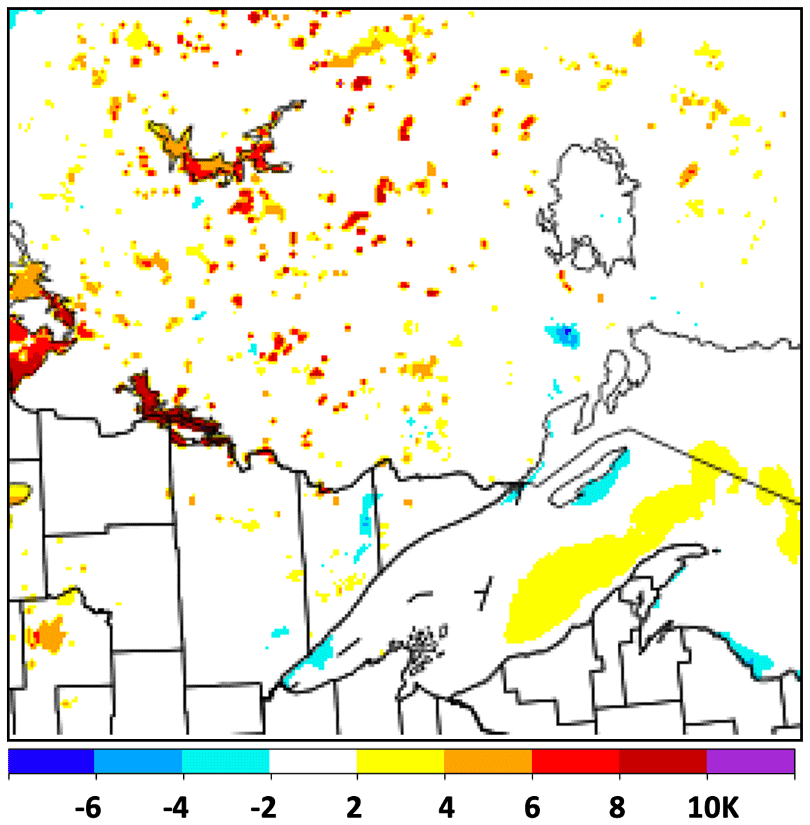
Figure 6 Difference (K) in lake surface temperatures between versions of HRRR model using cycled lake-model values (HRRRv4) and using interpolated NSST data (HRRRv3). Valid at 13:00 UTC on 13 October 2019 and also includes differences from use of the FVCOM lake model in HRRRv4 (Fujisaki-Manome et al., 2020).

5.2 Comparisons of different lake temperature estimates for 19 lakes from the lower 48 US and southern Canada during 2021

During a period from March to November 2021, a comparison was made of lake surface temperatures between the cycled HRRRv4-CLM values and those from three other estimates from NASA, NOAA, and in situ observations. A geographically diverse set of 19 lakes over the lower 48 United States and southern Canada was selected for these comparisons as listed in Table 5 and shown in Fig. 7. Lakes selected included near-ocean lagoon areas separated from ocean areas by coastal land as resolved by the 3 km land–water mask as discussed in Sect. 3.2. The water areas also included a reservoir (Lake Sakakawea). Some of these lakes are dimictic or polymictic (with ice cover part of each year, Lewis, 1983), but five of them do not experience any ice cover (Table 5), and lakes 5, 6, 7, and 8 are monomictic. The CLM lake model was cycled for all these lakes in the 3 km HRRRv4 model. The 19 lakes included 7 lakes with a surface area greater than 1000 km². The March–November evaluation period includes the spring–summer warming period and the cooling period in autumn. Data points were obtained monthly for March–August and weekly for September–November.

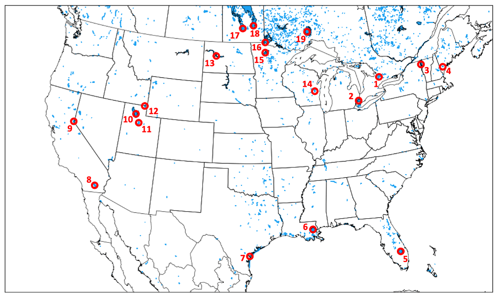
Figure 7 Locations of 19 lakes (see Table 5) used for the lake surface temperature intercomparison in this paper in Fig. 8. These lakes are shown as mapped onto the 3 km CONUS HRRR model domain.

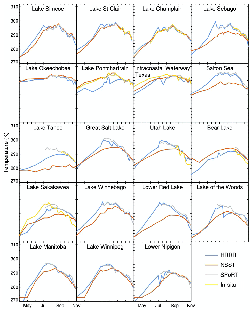
Figure 8 Lake surface temperatures in 2021 (April–October) from the 19 selected lakes (Table 5, Fig. 7) from HRRR–CLM-cycled, NSST, SPoRT, and in situ data.

Table 5 Lakes for comparison of lake surface temperatures between HRRRv4/CLM, NASA SPoRT, NSST, and in situ observations as shown in Figs. 7 and 8. Area is shown for lakes more than 1000 km². Lake depths are constant within each lake except for lakes 2, 3, and 18. See Fig. 4 for example map of lake depth used in HRRR. Specific HRRR I/J 3 km grid points (indicated in table) were selected from HRRR data for each lake.

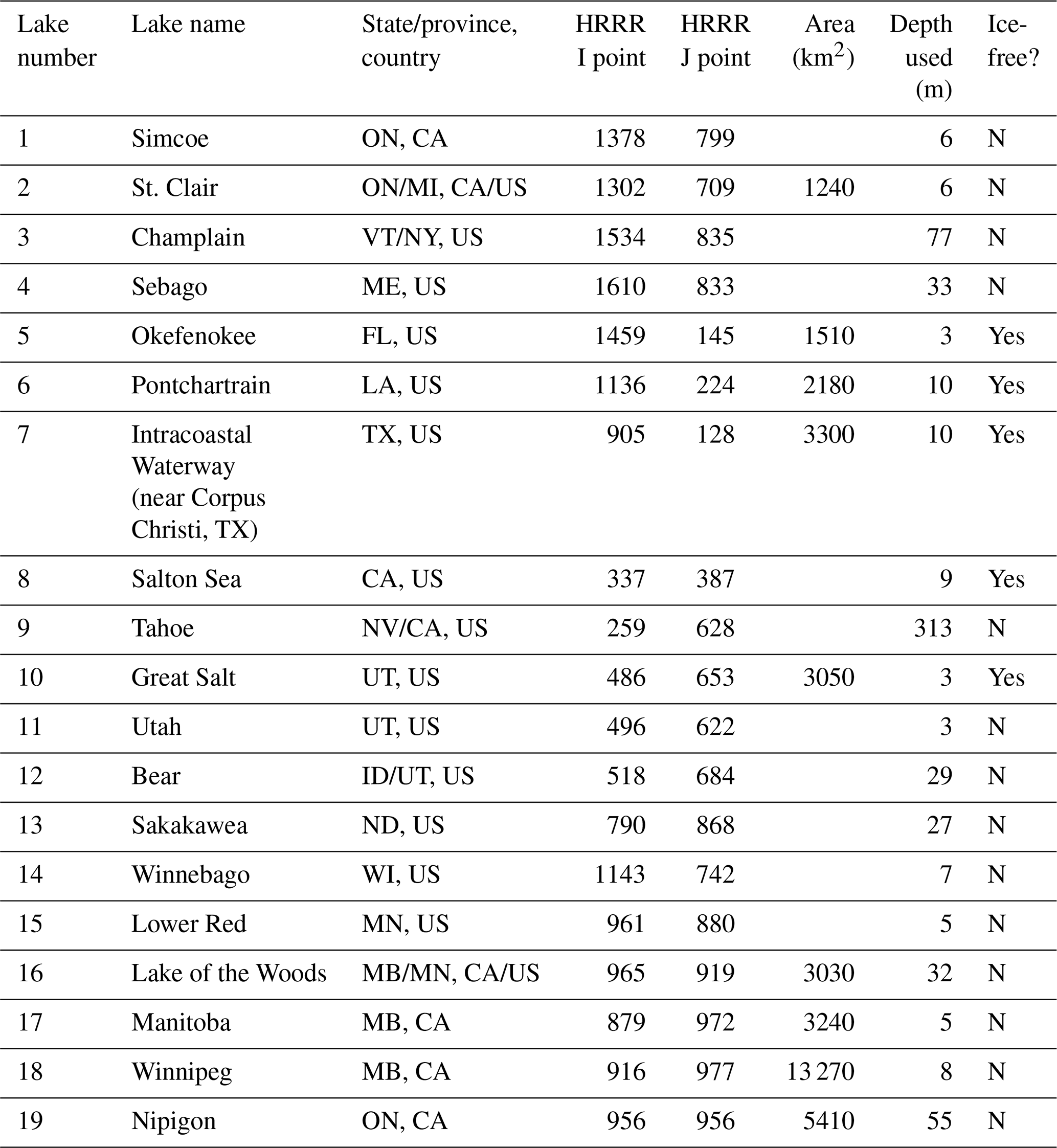
The HRRRv4-CLM values for these 19 lakes were compared first with an estimate from the NASA SPoRT (Short-term Prediction Research and Transition) real-time surface water temperature composite including time-weighted MODIS and VIIRS data for inland lakes (NASA, 2021; Kelley et al., 2021). The SPoRT estimates are similar to the satellite-based lake temperature estimates from the Met Office (Fiedler et al., 2014). The SPoRT composite is valid from the surface to 2 m depth and is averaged over a 7 d period to mitigate for cloud cover on a given day. A second lake temperature estimate is that from NSST, as discussed earlier. Third, in situ surface water temperature observations were available from observing platforms in 9 of the 19 lakes (Table 6). The platforms are operated by federal, state, and local government agencies and a regional ocean observing system. The depths of the water temperature observations were only available at four of the nine platforms. At these four sites, the depth ranged from 0.45 to 0.9 m.

Table 6 Sources of available in situ data among 19 lakes in Table 5.

In general, the HRRRv4-CLM-cycled lake surface temperatures showed the anticipated difference from NSST values (Fig. 8) with quicker summer warming from HRRR–CLM cycling for all lakes except the southern three lakes (5, 6, and 7 in Table 5, with lakes 6 and 7 essentially lagoons in close proximity to the ocean) and Bear Lake in UT/ID (Lake 12, 39 m depth). The NSST estimates were colder for spring through summer than HRRR values for 15 of the 19 lakes, a consequence from the NSST estimate via horizontal interpolation from deeper bodies of water.

For the nine lakes with in situ observations (Table 6), the HRRR–CLM-cycled lake temperatures are generally able to better capture weekly variability in summer and autumn months, associated with windy periods increasing mixing or relatively warm and cool weather periods or varying amounts of cloud cover. This can be seen, for example, at Utah Lake and the Intracoastal Waterway west of Padre Island in Texas (note cooling from passage of Hurricane Nicholas in mid-September). The most dramatic improvement of HRRR–CLM over NSST lake temperatures is seen at Lake Tahoe and lakes 14–19 in the northern region, with NSST estimates 5–10 K too cool. At two of the lakes with in situ observations, the Intracoastal Waterway (linked to the ocean) and Lake Pontchartrain, both lagoons linked to the ocean, NSST estimates are generally closer than HRRR–CLM to the observations.

HRRR–CLM lake surface temperatures matched in situ observations well for the northern lakes, usually within 1–2 K. In contrast, the lake temperature values from SPoRT were generally warmer than HRRR or in situ observations in the autumn period. The SPoRT observations showed a strong confirmation of HRRR–CLM-cycled lake temperatures for lakes in the western US (lakes 8–13) and most lakes in the northern areas (lakes 4, 14–19). Finally, the HRRR–CLM-cycled lake temperatures during this period often varied strongly from the NSST estimates, with differences of up to 5–10 K (largest difference with Red Lake, Lake 15). The effect of lake depth was evident with a faster transition to fully mixed lakes for shallow lakes (e.g., 5 m depth for Red Lake in MN, Lake 15 in Table 5) but subject to more temporal and horizontal variation for deeper lakes. Figure 9 showed a strong intralake variation of 7 K across Lake of the Woods (32 m depth) in the HRRR–CLM estimate, in contrast with very little variation (<1 K) across Red Lake. Due to a lack of high-resolution observations of lake surface temperatures, it is difficult to determine which intralake variations are more realistic. However, we think some of these intralake contrasts from HRRR–CLM may be exaggerated from actual values, possibly requiring a future introduction of a small temperature exchange rate (diffusion) between adjacent lake columns. Differences in skin temperature (e.g., SPoRT) and bulk temperature (e.g., in situ) for lakes have been noted (e.g., Wilson et al., 2013) of up to 0.5 K, but the HRRR vs. NSST differences in this study are generally much larger than this magnitude.

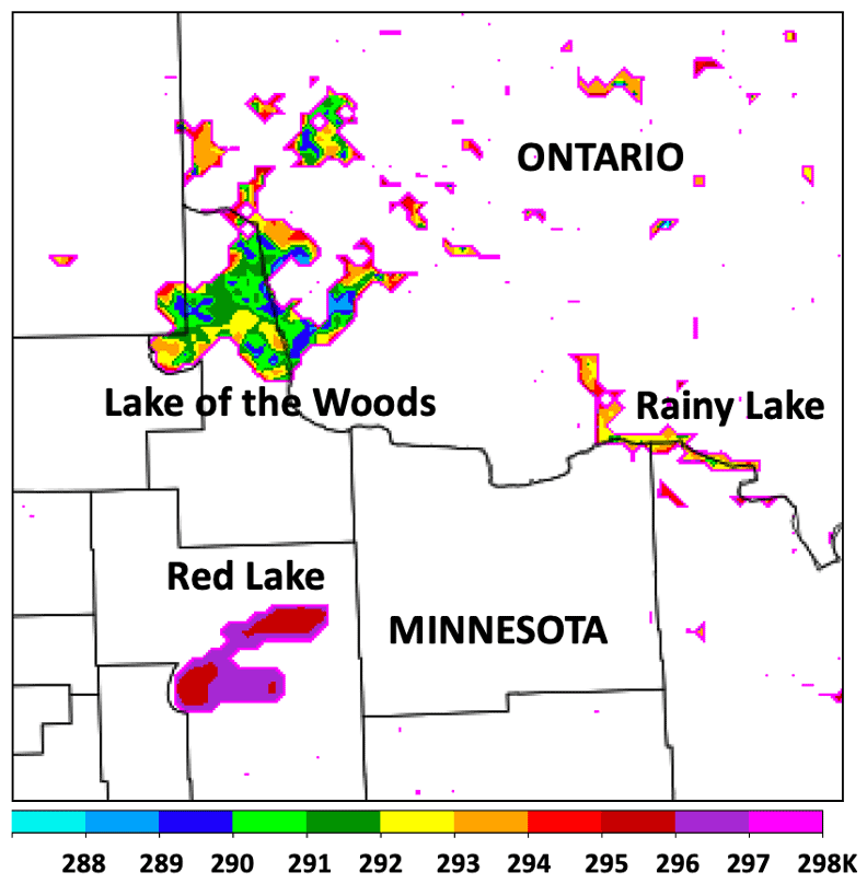
Figure 9 HRRRv4-CLM lake surface temperature (K) for 15:00 UTC on 31 July 2021 for the area over northern Minnesota (US) and southwestern Ontario (Canada).

The main deficiencies evident so far with the HRRR–CLM lake temperatures appear to be associated with errors in lake depth values. On the average, the current specified values for mean lake depth for most lakes are too deep compared to reality, since the preprocessing with the K12 dataset simply assigned a single lake depth value (maximum or mean) to all grid points for that lake even up to the modeled lake points adjacent to land, as shown in Table 5 for 16 or the 19 lakes studied. We also noted too-low lake temperatures in HRRRv4 for lake grid points at the western edge of a few lakes – e.g., Tahoe, Sebago (ME), Cayuga (NY), and Champlain, all relatively deep lakes (Fig. 5, Table 5). We attribute this to 1-D upwelling from insufficient bathymetry data resulting in cylinder-like lake volumes with constant lake depths, therefore with (a) too-deep lake-edge pixels coinciding with (b) strong winds coming off from land areas with predominantly westerly winds. This deficient effect was not widespread for the HRRR model and did not affect the overall results. Again, this behavior is attributed to the behavior of the lake model over integrations with the inaccurate lake depth information and not to the lake cycling initialization design.

6 Conclusions

We report here on the first use of a small-lake model (CLM4.5, 10 layer) in US NOAA NWP models along with an ongoing cycling of lake temperatures since 2018 to initialize lake temperatures in each prediction. These models are the 3 km HRRRv4 (D22, J22) and 13 km RAPv5 hourly updated models, both of which became operational in December 2020 after cycling since August 2018. At 3 km grid spacing, the HRRR model applied this small-lake modeling and assimilation to 1864 small lakes varying in size from about 10 km² (single grid point) to 14 larger lakes over 1000 km² in surface area but not including the Laurentian Great Lakes. The effectiveness of introducing the multi-layer lake model into the HRRR and RAP models was completely dependent on the initialization for lake temperatures. The introduction of a cycling capability through the hourly assimilation allowed the lake temperatures to evolve to accurate values, consistent with recent weather. In this paper, we describe the lake cycling applied for the NOAA regional 3 km HRRR and 13 km RAP weather models including the coupled 1-D CLM lake model. We also show some comparisons with other estimates of lake surface temperatures. From those comparisons, the cycled lake surface temperatures from the 3 km HRRR model were found to be reasonably accurate. HRRR lake surface temperatures were found to be generally within 1 K of in situ observations and within 2 K of the SPoRT estimates. Finally, NSST estimates of small-lake temperatures were found to often differ from in situ observations and HRRR estimates by 5–12 K. Other differences between lake-cycled HRRR estimates and SST-based estimates were up to 10–15 K.

From these initial results, we conclude that the lake-cycling initialization for small lakes has been effective overall, owing to accurate hourly estimates of near-surface temperature, moisture and winds, and shortwave and longwave estimates provided to the 1-D CLM lake model every time step (20 s for the 3 km HRRR model). The HRRR–CLM treatment also allows some inland lakes to freeze in winter, which is more consistent with observations. The lake cycling strategy is similar to that initialization method used by ECMWF for its 9 km (as of 2021) IFS (Integrated Forecast System) and using a binary lake mask in the 3 km HRRR model.

One deficiency noted was the development of a too-cold lake surface for a few lakes on their western boundary. We attribute this to the incorrect bathymetry data with constant lake depth (e.g., see caption for Table 5) causing an excessive 1-D upwelling from too-deep lake depth at the western shores for these lakes. This issue is being addressed with a current project to improve lake bathymetry data for which results will be reported in the future. Also, HRRR–CLM cycling gave poorer results than NSST at least for Lake Pontchartrain (Lake 6 in Table 5), suggesting to use NSST for near-ocean lagoon areas. More investigation is needed for strong intralake variations overall in HRRR–CLM-cycling representation (e.g., Lake of the Woods in Fig. 9) and possible introduction of horizontal diffusion of temperature between adjacent lake points.

US NWS forecasters have reported much improved near-surface temperature and dew point predictions in the vicinity of small lakes from the 3 km HRRR model in 2021 since the implementation of the 1-D CLM lake model and lake-cycling initialization. Again, this effort complements the coupling of the HRRR model with the 3-D FVCOM hydrodynamical lake model for the Laurentian Great Lakes (Fujisaki-Manome et al., 2020) design to improve lake-effect snow predictions. These efforts are the most advanced lake-coupling and lake-initialization efforts at this point in US NOAA weather models.

Overall, the improved lake temperatures from the lake cycling initialization technique driven over a 3-year period by accurate atmospheric conditions described here result in improved fluxes of heat and moisture over using SST interpolation and improved nearby predictions of atmospheric 2 m temperature and 2 m moisture.