the Creative Commons Attribution 4.0 License.
the Creative Commons Attribution 4.0 License.
 | 01 Sep 2022
A physically based distributed karst hydrological model (QMG model-V1.0) for flood simulations
Daoxian Yuan
Fuxi Zhang
Jiao Liu
Mingguo Ma
Karst trough and valley landforms are prone to flooding, primarily because of the unique hydrogeological features of karst landforms, which are conducive to the spread of rapid runoff. Hydrological models that represent the complicated hydrological processes in karst regions are effective for predicting karst flooding, but their application has been hampered by their complex model structures and associated parameter set, especially for distributed hydrological models, which require large amounts of hydrogeological data. Distributed hydrological models for predicting flooding are highly dependent on distributed modelling, complicated boundary parameter settings and extensive hydrogeological data processing, which consumes large amounts of both time and computational power. Proposed here is a distributed physically based karst hydrological model known as the QMG (Qingmuguan) model. The structural design of this model is relatively simple, and it is generally divided into surface and underground double-layered structures. The parameters that represent the structural functions of each layer have clear physical meanings, and fewer parameters are included in this model than in the current distributed models. This allows karst areas to be modelled with only a small amount of necessary hydrogeological data. Eighteen flood processes across the karst underground river in the Qingmuguan karst trough valley are simulated by the QMG model, and the simulated values agree well with observations: the average values of the Nash–Sutcliffe coefficient and the water balance coefficient are both 0.92, while the average relative flow process error is 10 % and the flood peak error is 11 %. A sensitivity analysis shows that the infiltration coefficient, permeability coefficient and rock porosity are the parameters that require the most attention in model calibration and optimization. The improved predictability of karst flooding enabled by the proposed QMG model promotes a better mechanistic depiction of runoff generation and confluence in karst trough valleys.
- Article
(1368 KB) - Full-text XML
- BibTeX
- EndNote


Karst trough and valley landforms are very common in China, especially in the southwest. In general, these karst areas are water scarce during most of the year because their surfaces store very little rainfall, but they are also potential origins of floods because their trough and valley landforms and topographic features facilitate the formation and propagation of floods (White, 2002; Li et al., 2021; Gautama et al., 2021). The coexistence of droughts and floods is a typical phenomenon in these karst trough and valley areas. Taking the example of the present study area, i.e. the Qingmuguan karst trough valley, floods used to happen constantly during the rainy season. In recent years, with more extreme rainfall events and the increased area of construction land in the region, rainfall infiltration has decreased, and rapid runoff over impervious surfaces has increased, resulting in frequent catastrophic flooding in the basin (Liu et al., 2009). Excess infiltration runoff from karst sinkholes and underground river outlets often occurs during flooding (Jourde et al., 2007, 2014; Martinotti et al., 2017), flooding large areas of farmland and residential areas and causing serious economic losses (Gutierrez, 2010; Parise, 2010; Yu et al., 2020). Therefore, it is both important and urgently necessary to simulate and predict karst flooding events in karst troughs and valleys such as those in the study area.
Hydrological models can be effective for forecasting floods and evaluating water resources in karst areas (Bonacci et al., 2006; Williams, 2008, 2009). However, modelling floods in karst regions is extremely difficult because of the corresponding complex hydrogeological structures. Karst water-bearing systems consist of multiple media under the influence of complex karst development dynamics (Kovács and Perrochet, 2008; Gutierrez, 2010), such as karst caves, conduits, fissures and pores, and are usually highly spatially heterogeneous (Chang and Liu, 2015; Teixeiraparente et al., 2019; Zhang, 2021). In addition, the intricate surface hydrogeological conditions and the hydrodynamic conditions inside the karst water-bearing medium result in significant temporal and spatial differences in the hydrological processes in karst areas (Geyer et al., 2008; Bittner et al., 2020; Jamal and Awotunde, 2022).
In early studies of flood forecasting in karst regions, simplified lumped hydrological models were commonly used to describe the rainfall–discharge relationship (e.g. Kovács and Sauter, 2008; Fleury et al., 2007; Jukić and Denić-Jukić, 2009; Hartmann et al., 2014). With the development of physical exploration technology and progress in mathematics, computing and other interdisciplinary disciplines, the level of modelling has gradually improved (Hartmann and Baker, 2017; Hartmann, 2018; Petrie et al., 2021), and distributed hydrological models have subsequently become widely applied to karst areas. The main difference between lumped and distributed hydrological models is that the latter divide the entire basin into many subbasins to calculate the runoff generation and confluence (Chang et al., 2021; Guila et al., 2022), thereby better describing the physical properties of the hydrological processes inside a karst water-bearing system (Jourde et al., 2007; Hartmann, 2018; Epting et al., 2018).
Because of their simple structure and low demands for modelling data, lumped hydrological models have been used widely in karst areas (Kurtulus and Razack, 2007; Ladouche et al., 2014). In a lumped model, a river basin is considered as a whole in the calculation of the runoff generation and confluence, and there is no division into subbasins (Dewandel et al., 2003; Bittner et al., 2020). Lumped models usually consider the inputs and outputs of the model (Liedl et al., 2003; Hartmann and Baker, 2013, 2017). In addition, most of the model parameters in a lumped model are not optimized, and the physical meaning of each parameter is unclear (Chen et al., 2010; Bittner et al., 2020).
Distributed hydrological models are of active interest in flood simulation and forecasting research (Ambroise et al., 1996; Beven and Binley, 2006; Zhu and Li, 2014). Compared with that of a lumped model, the structure of a distributed model has a more definite physical significance in terms of its mechanism (Meng and Wang, 2010; Epting et al., 2018). In a distributed hydrological model, an entire karst basin can be divided into many subbasins (Birk et al., 2005) using high-resolution digital elevation model (DEM) data. In the rainfall-runoff algorithm of the model, the hydrogeological conditions and karst aquifer characteristics can be considered fully to precisely simulate the runoff generation and confluence (Martinotti et al., 2017; Gang et al., 2019). The commonly used basin distributed hydrological models (i.e. not special groundwater numerical models such as MODFLOW) have also been widely applied to karst areas and include the SHE/MIKE and SHE models (Abbott et al., 1986a, b; Doummar et al., 2012), the Storm Water Management Model (SWMM) (Peterson and Wicks, 2006; Blansett and Hamlett, 2010; Blansett, 2011), the TOPography-based hydrological MODEL (TOPMODEL) (Ambroise et al., 1996; Suo et al., 2007; Lu et al., 2013; Pan, 2014) and the Soil and Water Assessment Tool (SWAT) (Peterson and Hamlett, 1998).
The commonly used distributed hydrological models include multiple structures and numerous parameters (Lu et al., 2013; Pan, 2014; Masciopinto et al., 2021), which means that vast amounts of data may be needed to build the model framework in karst regions. For example, the distributed groundwater model MODFLOW-CFPM1 requires detailed data regarding the distribution of karst conduits in the study area (Reimann and Hill, 2009). Another example is the Karst–Liuxihe model (Li et al., 2019); there are 15 parameters and 5 underground vertical structures in this model. Such a complex structure results in large modelling-data demands, and modelling in karst areas is extremely difficult. In addition, a special borehole pumping test may be required to obtain the rock permeability coefficient.
To overcome the difficulty posed by the large modelling-data demands of distributed hydrological models in karst areas, a new physically based distributed hydrological model – known as the QMG (Qingmuguan) model-V1.0 – was developed in the present study. Other commonly used karst groundwater models with complex structures and parameters, such as the aforementioned MODFLOW-CFPM1 model, require considerable hydrogeological data for modelling in karst areas (Qin and Jiang, 2014). The new QMG model has a high potential for application in karst hydrological simulation and prediction. It has certain advantages in terms of its framework and structural design, with a double-layer structure and fewer parameters. The horizontal structure is divided into river channel units and slope units, and the vertical structure below the surface is divided into a shallow karst aquifer and a deep karst aquifer system. This relatively simple model structure reduces the demand for modelling data in karst areas, and only a small amount of hydrogeological data is needed for modelling. To ensure that the QMG model works well in karst flood simulation and prediction despite its relatively simple structure and parameters, we carefully designed the algorithms for runoff generation and confluence in the model. Additionally, to verify the applicability of the QMG model to flood simulation in karst basins, we selected the Qingmuguan karst trough valley in Chongqing, China, as the study area for flood simulation and uncertainty analysis. In particular, we analysed the sensitivity of the model parameters.
2.1 Landform and topography
The Qingmuguan karst trough valley is located in the southeastern part of the Sichuan Basin, China, at the junction of the Beibei and Shapingba districts in Chongqing, with coordinates of 29∘40′–29∘47′ N, 106∘17′–106∘20′ E. The basin covers an area of 13.4 km2 and is part of the southern extension of the anticline at Wintang Gorge in the Jinyun Mountains, with the anticlinal axis of Qingmuguan located in a parallel valley in eastern Sichuan (Yang et al., 2008). The surface of the anticline is heavily fragmented, and faults are extremely well developed, with large areas of exposed Triassic carbonate rocks. Under the long-term erosion of karst water, a typical karst trough landform developed (Liu et al., 2009). This karst trough landform provides convenient conditions for flood propagation, and the development of karst landforms is extremely common in the karst region of southwestern China, especially in the karst region of Chongqing.
The basin is oriented in a narrow band of slightly curved arcs and is ∼12 km long from north to south. The direction of the mountains in the region is generally consistent with the direction of the tectonic line. The catchment area of the basin is mainly composed of the outlying areas of the Lower Triassic Jialingjiang Formation (T1j), the middle Leikoupo Formation (T2l) carbonate rocks on both sides of the mountain slopes, and part of the Upper Xujiahe Formation (T3xj) quartz-sandstone and mudstone (Yang et al., 2008). Tracer tests show that karst development in the underground river system in the study area is strong, where the karst water-bearing medium is heterogeneous and has high water permeability. A large-scale underground river (Fig. 1) with a length of approximately 7.4 km has developed in the karst trough valley, and the flood peak flow of this underground river lasts for a short time.
The karst landforms in the area are well developed under closed conditions, and precipitation is the main source of recharge for the underground river system. Most of the precipitation, after evapotranspiration and plant retention are deducted, collects along the slope to the depression at the bottom of the trough and joins the underground river through surface karst fissure dispersion infiltration and concentrated injection in the sinkholes. The map in Fig. 1 gives an overview of the Qingmuguan karst basin.
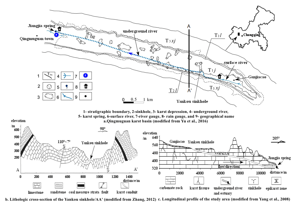
Figure 1The Qingmuguan karst basin.
2.2 Hydrogeological conditions
The Qingmuguan basin is located within a subtropical humid monsoon climate zone, with an average temperature of 16.5 ∘C and an average precipitation of 1250 mm concentrated mainly in May–September. An underground river system with a length of 7.4 km has developed in the karst trough valley, and the water supply of the underground river is mainly rainfall recharge (Zhang, 2012). Most of the precipitation is collected along the hill slope and routed into the karst depressions at the bottom of the trough valley, where it joins the underground river through the dispersed infiltration of surface karst fissures and sinkholes (Fig. 1a). An upstream surface river collects in a gentle valley and enters the underground river through the Yankou sinkhole (elevation 524 m). Surface water in the middle and lower reaches of the river system enters the underground river system mainly through cover collapse sinkholes (Gutierrez et al., 2014) or fissures.
The stratigraphic and lithologic characteristics of the basin are dominated largely by carbonate rocks of the Lower Triassic Jialingjiang Group (T1j) and Middle Triassic Leikou Slope Group (T2l) on both sides of the slope, with some quartz sandstone and mudstone outcrops of the Upper Triassic Xujiahe Group (T3xj) (Zhang, 2012). The topography of the basin presents a general anticline (Fig. 1b), where carbonate rocks on the surface are corroded and fragmented and have high permeability. Compared with the core of the anticline, the shale of the anticline is less eroded and forms a good waterproof layer.
To investigate the distribution of karst conduits in the underground river system, we conducted a tracer test in the study area. The tracer was placed in the Yankou sinkhole and recovered in the Jiangjia spring (Fig. 1a and c). According to the tracer test results (Gou et al., 2010), the karst water-bearing medium in the aquifer was anisotropic, the karst conduits in the underground river were extremely well developed, and there was a large single-channel underground river approximately 5 m wide. The response of the underground river to rainfall was very fast, with the peak flow observed at the outlet of the Jiangjia spring 6–8 h after rainfall based on the tracer test results. The flood peak rose quickly, and the duration of the peak flow was short. The underground river system in the study area is dominated by large karst conduits, which are not conducive to water storage in water-bearing media but are very conducive to the propagation of floods.
2.3 Modelling data
To build the QMG model to simulate karst flood events, the necessary baseline modelling data had to be collected, including (1) high-resolution DEM data and hydrogeological data (e.g. the thickness of the epikarst zone, rainfall infiltration coefficients of different karst landforms, and the rock permeability coefficient); (2) land-use and soil-type data; and (3) rainfall data in the basin and water flow data for the underground river. The DEM data were downloaded from a free database on the public internet, with an initial spatial resolution of 30×30 m. The spatial resolution of the land use and soil types was 1000×1000 m, and they were also downloaded from the internet. After the applicability of modelling and computational strength, as well as the size of the basin in the study area (13.4 km2), was considered, the spatial resolution of the three types of data was resampled uniformly in the QMG model and downscaled to 15×15 m based on a spatial discrete method by Berry et al. (2010).
The hydrogeological data necessary for modelling were obtained in three simple ways. (1) A basin survey was conducted to obtain the thickness of the epikarst zone, which was achieved by observing the rock formations on hillsides following cutting for road construction. Information was collected regarding the location, general shape and size of karst depressions and sinkholes, which had a significant impact on the compilation of the DEM data and the determination of the convergence process of surface runoff. The sinkholes in the basin are cover collapse sinkholes (Gutierrez et al., 2014) according to the basin survey. There are 3 large sinkholes (more than 3 m in diameter) and 12 small sinkholes (less than 1 m in diameter). The remaining 5 sinkholes are between 1 and 3 m in diameter. The confluence calculation of these sinkholes in the model was based on the results of a previous study (Meng et al., 2009). (2) Empirical equations developed for similar basins were used to obtain the rainfall infiltration coefficients for different karst landforms and the rock permeability coefficient. For example, the rock permeability coefficient was calculated based on an empirical equation from a pumping test in a coal mine in the study area (Li et al., 2019). (3) A tracer experiment was conducted in the study area (Gou et al., 2010) to obtain information on the underground river direction and flow velocity; for instance, underground karst conduits are well developed in the area and form an underground river approximately 5 m wide. There are no hydraulic connections between the underground river system in the area and the adjacent basin, which means that there is no overflow recharge.
Rainfall and flood data are important model inputs and represent the driving factors that allow hydrological models to operate. In the study area, rainfall data were acquired by two rain gauges located in the basin (Fig. 1a). Point rainfall values were then spatially interpolated into basin-level rainfall (for such a small basin area, rainfall results obtained from two rain gauges were considered representative). There were 18 karst flood events from 14 April 2017 to 10 June 2019. We built a rectangular open channel at the underground river outlet and set up a river gauge in it (Fig. 1a) to record the water level and flow data every 15 min.
3.1 Hydrological model
The hydrological model developed in this study was named the QMG model after the basin for which it was developed and to which it was first applied, i.e. the Qingmuguan basin. The QMG model has a two-layer structure, including a surface part and an underground part. The surface structure is mainly used to perform the calculation of runoff generation and the confluence of the surface river, while the underground structure is used to perform the confluence calculation of the underground river system.
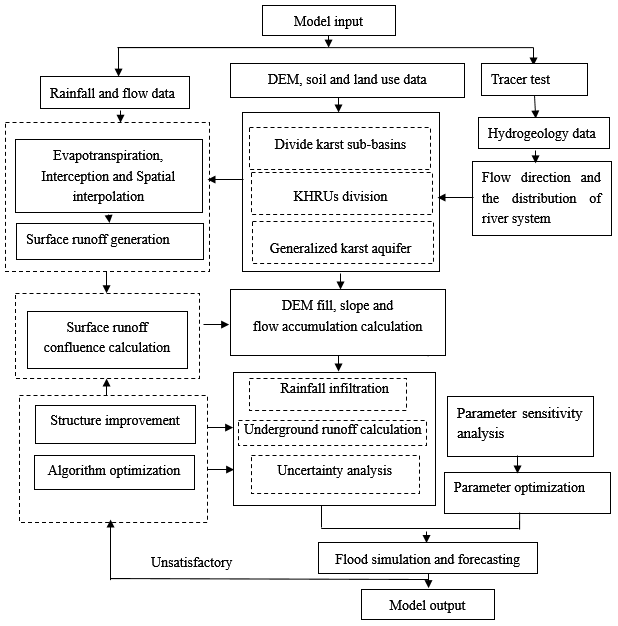
The structure of the QMG model is divided into a two-layer structure, both horizontally and vertically. The horizontal structure of the model is divided into river channel units and slope units. The vertical structure below the surface is divided into a shallow karst aquifer (including soil layers, karst fissures and conduit systems in the epikarst zone) and a deep karst aquifer system (bedrock and the underground river system). This relatively simple model structure means that only a small amount of hydrogeological data is needed in karst regions. Figure 2 shows a flowchart of the modelling and calculation procedures required for the QMG model.
To accurately describe the runoff generation and confluence on a grid scale, these karst subbasins are further divided into many karst hydrological response units (KHRUs) based on the high-resolution (15×15 m) DEM data in the model. The specific steps involved in the division were adopted by referring to studies of hydrological response units (HRUs) in TOPMODEL by Pan (2014). The KHRUs are the smallest basin computing units; the spatial differences in karst development within the units can be effectively ignored, and the use of these units reduces the uncertainty in the model unit classification. Figure 3 shows the spatial structure of the KHRUs.
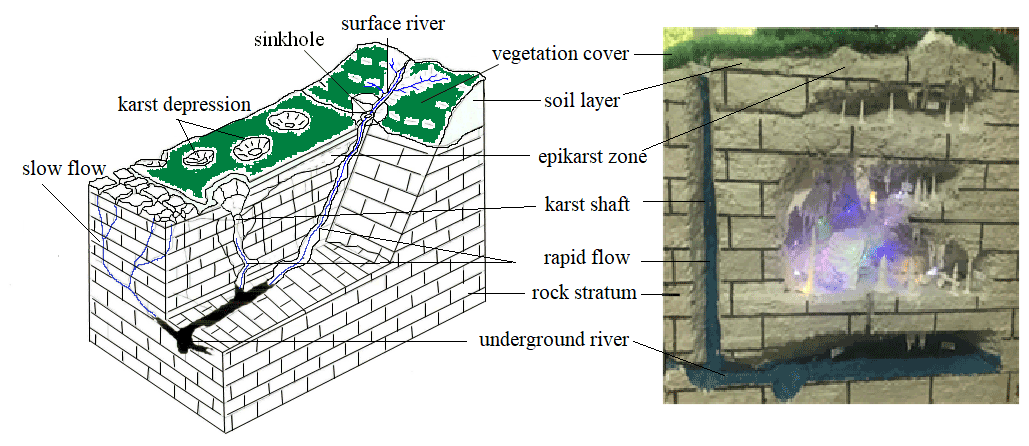
The right-hand side of Fig. 3 shows a three-dimensional spatial model of KHRUs established in the laboratory to visually reflect the storage and movement of water in the karst water-bearing medium with each spatially anisotropic component and to provide technical support for establishing the hydrological model.
The modelling and operation of the QMG model consists of three main stages: (1) spatial interpolation and the retention of rainfall and evaporation calculations; (2) runoff generation and confluence calculation for the surface river; and (3) confluence calculation for the underground runoff, including the confluence in the shallow karst aquifer and the underground river system.
3.1.1 Rainfall and evaporation calculation
In the QMG model, the spatial interpolation of rainfall is accomplished by a kriging method using ArcGIS 10.2 software. The Tyson polygon method may be a simpler method for rainfall interpolation if the number of rainfall gauges in the basin is sufficient. The point rainfall values observed by the two rainfall gauges in the basin (Fig. 1a) were interpolated spatially into an areal rainfall for the entire basin.
Basin evapotranspiration in the KHRUs was mainly vegetal evaporation, soil evaporation and water surface evaporation. These components were calculated using the following equations (modified from Li et al., 2020):
Here, Ev [mm] is the vegetal discharge, [mm] is the rainfall variation due to vegetation interception, Pv [mm] is the vegetation interception of rainfall and Es [mm] is the actual soil evaporation. The term λ is the evaporation coefficient. The term Ep [mm] is the evaporation capability, which can be measured experimentally or estimated by the water surface evaporation equation Ew. The term F [mm] is the actual soil moisture, Fsat [mm] is the saturation moisture content, Fc [mm] is the field capacity, Ew [mm d−1] is the evaporation of the water surface, and [hPa] is the draught head between the saturation vapour pressure of the water surface and the air vapour pressure 150 m above the water surface. The term [∘C] is the temperature difference between the water surface and the temperature 150 m above the water surface, γ is the relative humidity 150 m above the water surface, and ω [m s−1] is the wind speed 150 m above the water surface.
3.1.2 Runoff generation algorithms
In the QMG model, the surface runoff generation in river channel units is the rainfall in the river system after evaporation losses are deducted. This portion of the runoff directly participates in the confluence process through the river system rather than undergoing infiltration. In contrast, the process of runoff generation in slope units is more complex, and its classification is related to the developmental characteristics of the surface karst in the basin, rainfall intensity and soil moisture. For example, when the soil moisture content is already saturated, there is the potential for excess infiltration surface runoff in exposed karst slope units. The surface runoff generation of the KHRUs in the river channel units and slope units can be described by the following equations (modified from Chen et al., 2010; Li et al., 2020):
Here, Pr(t) [mm] is the net rainfall (deducting evaporation losses) in the river channel units at time t [h], Pi(t) [mm] is the rainfall in the river channel units, L [m] is the length of the river channel, Wmax [m] is the maximum width of the river channel selected, and A [m2] is the cross-sectional area of the river channel. Rsi [mm] is termed the excess infiltration runoff in the QMG model when the vadose zone is short of water and has not been filled. The infiltration capacity fmax is different for different karst landform units, α and β are the parameters of the Holtan model, and Fs [mm] is the stable depth of soil water infiltration.
In the KHRUs (Fig. 3), underground runoff is generated primarily from the infiltration of rainwater and direct confluence recharge from sinkholes or skylights. In the QMG model, the underground runoff is calculated by the following equations (modified from Chen, 2018):
where
Here, Rg [mm] is the underground runoff depth (this part of the underground runoff is mainly from the direct confluence supply of the karst sinkholes or karst windows in the study area), R0 [mm] is the average depth of the underground runoff, p and m are attenuation coefficients calculated by conducting a tracer test in the study area, Re [L s−1] is the underground runoff generated from rainfall infiltration in the epikarst zone, Iw [mm] is the width of the underground runoff on the KHRUs, z [mm] is the thickness of the epikarst zone, Rr [mm2 s−1] is the runoff recharge on the KHRUs during period t, Repi [mm2 s−1] is the water infiltration from rainfall, ve [mm s−1] is the flow velocity of the underground runoff, K [mm s−1] is the current permeability coefficient, and α is the hydraulic gradient of the underground runoff. If the current soil moisture is less than the field capacity, i.e. F≤Fc, then the vadose zone is not yet full, no underground runoff is generated, and rainfall infiltration at this time continues to compensate for the lack of water in the vadose zone until it is full and before runoff is generated.
3.1.3 Confluence algorithms
In the QMG model, the calculation of the runoff confluence on the KHRUs includes the confluence of the surface river channel and underground runoff. There are already many mature and classical algorithms available for calculating the runoff confluence in river channel units and slope units, such as the Saint-Venant equations and Muskingum convergence model. In this study, the Saint-Venant equations were adopted to describe the confluence in the surface river and hill slope units, for which a wave movement equation was adopted to calculate the confluence in slope units (Chen et al., 2010):
where
Here, we customized two variables, a and b:
Equation (7) was substituted into Eq. (5) and discretized by a finite-difference method, giving
The Newton–Raphson method was used for iterative calculation using Eq. (9):
where Q [L s−1] is the confluence of water flow in slope units, L [dm] is its runoff width, h [dm] is the runoff depth and q [dm2 s−1] is the lateral inflow on the KHRUs. Here, the friction slope Sf equals the hill slope S0, and the inertia term and the pressure term in the motion equation of the Saint-Venant equations were ignored. The term v [dm s−1] is the flow velocity of surface runoff in the slope units as calculated by the Manning equation, n is the roughness coefficient of the slope units, [L s−1] is the slope inflow in the KHRU at time t+1, and [L s−1] is the slope discharge in the upper adjacent KHRU at time t+1.
Similarly, the surface river channel confluence was described based on the Saint-Venant equation, where a diffusion wave movement equation was adopted, meaning that the inertia term in the motion equation was ignored:
A finite-difference method and the Newton–Raphson method were used for the iterative calculation of the above equation:
where Q [L s−1] is the water flow in surface river channel units, A [dm2] is the discharge section area, c is a custom intermediate variable and χ [dm] is the wetted perimeter of the discharge section area.
The underground runoff in the model includes the confluence of the epikarst zone and underground river. In the epikarst zone, the karst water-bearing media are highly heterogeneous (Williams, 2008). For example, anisotropic karst fissure systems and conduit systems consist of corrosion fractures. When rainfall infiltrates the epikarst zone, water moves slowly through the small (smaller than 10 cm in this study) karst fissure systems, while it flows rapidly in larger (larger than 10 cm) conduits. The key to determining the confluence velocity lies in the width of karst fractures. In the KHRUs (Fig. 3), a fracture width of 10 cm was used as a threshold value (Atkinson, 1977) based on a borehole pumping test in the basin, meaning that if the fracture width exceeded 10 cm, then the water movement into it was defined as rapid flow; otherwise, it was defined as slow flow. The confluence in the epikarst zone was calculated by the following equation (modified from Beven and Binley, 2006):
where
Here, Q(t)ijk [L s−1] is the flow confluence in the epikarst zone at time t, bijk [dm] is the runoff width, is the dimensionless hydraulic gradient, is the dimensionless hydraulic conductivity, ρ [g L−1] is the density of the water flow, g [m s−2] is gravitational acceleration, n is the number of valid computational units, RiCjLk [L] is the volume of the ijkth KHRU, v is the kinematic viscosity coefficient, fij is the attenuation coefficient in the epikarst zone, hij [dm] is the depth of shallow groundwater, and zij [dm] is the thickness of the epikarst zone.
The distinction between rapid and slow flows in the epikarst zone is not absolute. The choice of a 10 cm width karst fracture as the dividing threshold is based on limited evidence because only five limited boreholes have been tested for pumping in the region. In fact, there is usually water exchange between the rapid and slow flows at the junction of large and small fissures in karst aquifers. In the QMG model, this water exchange can be described with the following equation (modified from Li et al., 2021):
Here, [dm2 s−1] is the water exchange coefficient of the ijkth KHRU, [dm] is the water head difference between rapid and slow flows at the junction of large and small fissures in KHRUs, np is the number of fissure systems connected to the adjacent conduit systems, [dm s−1] is the permeability coefficient at the junction of a fissure and conduit, dip and rip [dm] are the conduit diameter and radius, respectively, Δlip [dm] is the length of the connection between conduits i and p, and τip is the conduit curvature. Some of the parameters in this equation, such as and , were obtained by conducting an infiltration test in the study area.
The confluence of the underground river system plays an important role in the confluence at the basin outlet. To facilitate the calculation of the confluence in the QMG model, the underground river systems can be generalized into large multiple conduit systems. During flooding, these conduit systems are mostly under pressure. Whether the water flow is laminar or turbulent depends on the flow regime at that time. The water flow into these conduits is calculated by the Hagen–Poiseuille equation and the Darcy–Weisbach equation (Shoemaker et al., 2008):
Here, Qlaminar [L s−1] is the water flow of the laminar flow in the conduit systems, A [dm2] is the conduit cross-sectional area, d [dm] is the conduit diameter, ρ [kg dm−3] is the density of the underground river, is the coefficient of kinematic viscosity, is the hydraulic slope of the conduits, τ is the dimensionless conduit curvature, Qturbulent [L s−1] is the turbulent flow in the conduit systems, and Hc [dm] is the average conduit wall height.
3.2 Parameter optimization
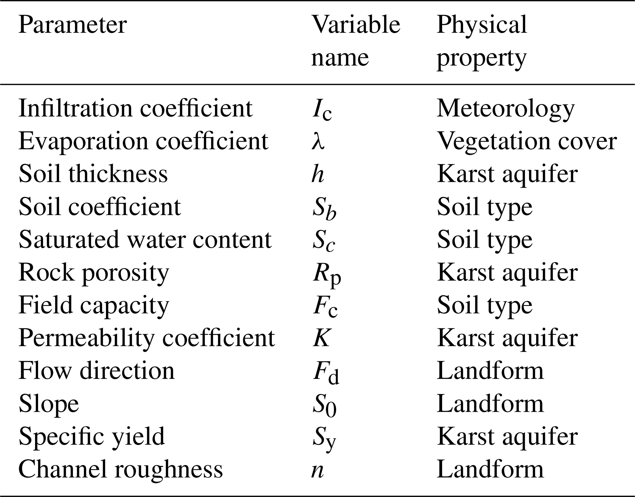
In total, the QMG model includes 12 parameters, among which flow direction and slope are topographic parameters that can be determined from the DEM without parametric optimization while the remaining 10 parameters require calibration. Other distributed hydrological models with multiple structures usually have many parameters. For example, the Karst–Liuxihe model (Li et al., 2021) has 15 parameters that must be calibrated. In the QMG model, each parameter is normalized as
where xi is the dimensionless parameter value i after it is normalized, x∗i is the parameter value i in actual physical units, and xi0 is the initial or final value of xi. Through the processing of Eq. (16), the value range of the model parameters is limited to a hypercube , i=1, 2, …, n), where K is a dimensionless value. This normalized treatment ignores the influence of the spatiotemporal variation in the underlying surface attributes on the parameters while also simplifying the classification and number of model parameters to a certain extent. Accordingly, the model parameters can be further divided into rainfall-evaporation parameters, epikarst-zone parameters and underground river parameters. Table 1 lists the parameters of the QMG model.
Because the QMG model has relatively few parameters, it is possible to calibrate them manually, which means that the operation is easy to implement and does not require a special programme for parameter optimization. However, the choice of parameters is subjective, which can lead to great uncertainty in the manual parameter calibration process. To compare the effects of parameter optimization on model performance, this study used both manual parameter calibration and the improved chaotic particle swarm optimization (ICPSO) algorithm for the automatic calibration of model parameters and compared the effects of both on flood simulation.
In general, the structure and parameters of a standard particle swarm optimization (PSO) algorithm are simple, with the initial parameter values obtained at random. For parameter optimization in high-dimensional multipeak hydrological models, the standard PSO is easily limited to local convergence and cannot achieve the optimal effect, while the late evolution of the algorithm may also cause problems, such as premature convergence and stagnant evolution, due to the “inert” aggregation of particles, which seriously affects the efficiency of parameter selection. It is necessary to overcome the above problems and to facilitate a high probability of algorithm convergence to the global optimal solution. In parameter optimization for the QMG model, we improved the standard PSO algorithm by adding chaos theory and developed the ICPSO, where 10 cycles of chaotic disturbances were added to improve the activity of the particles. The inverse mapping equation of the chaotic variable is
where Xij is the optimization variable for the model parameters and (Xmax−Xmin) is the difference between its maximum and its minimum; Zij is the variable before the disturbance is added and represents the chaotic variables after a disturbance is added; α () is a variable determined by the adaptive algorithm; and Z∗ is the chaotic variable formed when the optimal particle is mapped to the interval [0,1]. The flowchart of the ICPSO for parameter optimization is shown in Fig. 4.
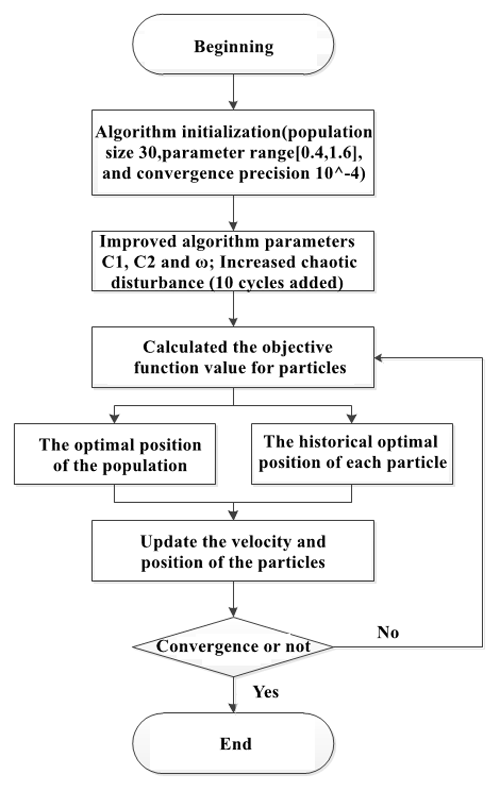
Figure 4Algorithm flow chart of the improved chaotic particle swarm optimization (ICPSO).
3.3 Uncertainty analysis
Uncertainties in hydrological model simulation results usually originate from three aspects: input data, model structure and model parameters (Krzysztofowicz, 2014). In the present study, the input data (e.g. rainfall, flood events and some hydrogeological data) were first validated and preprocessed through observations to reduce their uncertainties.
Second, we simplified the structure of the QMG model to reduce the structural uncertainty. As it is a mathematical and physical model, a hydrological model has some uncertainty in flood simulation and prediction because of the errors in system structure and the algorithm (Krzysztofowicz and Kelly, 2000). The model was designed with full consideration of the relationship between the amount of data required to build the model and its performance for flood simulation and prediction in karst regions, and the model's entire framework was integrated through simple structures and easy-to-implement algorithms using the concept of distributed hydrological modelling. Conventionally, the extent of uncertainty increases with the growing complexity of the model structure. We therefore ensured that the structure of the QMG model was simple when it was designed, and the model was divided into surface and underground double-layer structures to reduce its structural uncertainty.
Third, we focused on analysing the uncertainty and sensitivity of the model parameters and their optimization method, for which a multiparametric sensitivity analysis method (Li et al., 2020) was used to analyse the sensitivity of the parameters in the QMG model. The steps in the parameter sensitivity analysis were as follows.
-
Selection of the appropriate objective function.
The Nash–Sutcliffe coefficient is widely used as an objective function to evaluate the performance of hydrological models (Li et al., 2020, 2021). The coefficient was therefore used to assess the QMG model. Because the most important factor in flood prediction is the peak discharge, it is used in the Nash–Sutcliffe coefficient equation:
where NSC is the Nash–Sutcliffe coefficient, Qi [L s−1] represents the observed flow discharges, [L s−1] represents the simulated discharges, [L s−1] is the average observed discharge and n [h] is the observation period.
-
Parameter sequence sampling.
The Monte Carlo sampling method was used to sample 8000 groups of parameter sequences. The parametric sensitivity of the QMG model was analysed and evaluated by comparing the differences between the a priori and a posteriori distributions of the parameters.
-
Parameter sensitivity assessment.
The a priori distribution of a model parameter is its probability distribution, while the a posteriori distribution refers to the conditional distribution calculated after sample sampling and can be calculated based on the parametric optimization simulation result. If there is a significant difference between the a priori distribution and the a posteriori distribution of a parameter, then the parameter being tested has a high sensitivity, whereas if there is no obvious difference, then the parameter is insensitive. The parametric a priori distribution is calculated as follows:
where Pi,j is the a priori distribution probability when . We used a simulated Nash–Sutcliffe coefficient of 0.85 as the threshold value, and n was the number of occurrences of a Nash–Sutcliffe coefficient greater than 0.85 in flood simulations. In each simulation, only a certain parameter was changed, while the remaining parameters remained unchanged. If the Nash–Sutcliffe coefficient of this simulation exceeded 0.85, then the flood simulation results were considered acceptable. The term σi is the difference between the acceptable value and its mean, which represents the parametric sensitivity (). The higher the σi value is, the more sensitive the parameter. N is the 8000 parameter sequences, and is the average value of the a priori distribution.
3.4 Model setting
Once the model was built, some of the initial conditions had to be set before running it to simulate and forecast floods, such as basin division, the setting of initial soil moisture, and the assumption of the initial parameter range. (1) In the study area, the entire Qingmuguan karst basin was divided into 893 KHRUs, including 65 surface river units, 466 hill slope units and 362 underground river units. The division of these units formed the basis for calculating the process of runoff generation and convergence. (2) The initial soil moisture was set to 0 %–100 % of the saturation moisture content in the basin, and the specific soil moisture before each flood had to be determined by a trial calculation. (3) The waterhead boundary conditions of the groundwater were determined by a tracer test in the basin, where a perennial stable water level adjacent to the groundwater-divide was used as the fixed waterhead boundary. The base flow of the underground river was determined to be 35 L s−1 from the perennial average dry season runoff. (4) The ranges of initial parameters and convergence conditions were assumed before parameter optimization (Fig. 4). (5) Parameter optimization and flood simulation validated the performance of the QMG model in karst basins.
4.1 Parameter sensitivity results
The number of parameters in a distributed hydrological model is generally large, and it is important to perform a sensitivity analysis on each parameter to quantitatively assess the impacts of the different parameters on model performance. In the QMG model, each parameter was placed into one of four categories according to its sensitivity: (i) highly sensitive, (ii) sensitive, (iii) moderately sensitive and (v) insensitive. In the calibration of model parameters, insensitive parameters do not need to be calibrated, which can greatly reduce the number of calculations and improve the model operation efficiency.
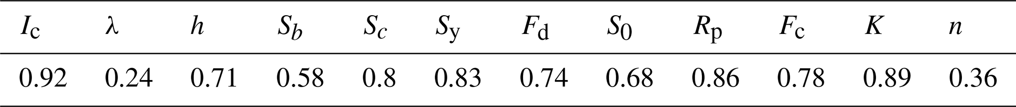
The flow process in the calibration period (14 April to 10 May 2017) was adopted to calculate the sensitivity of the model parameters, where Eq. (19) was used, and the parameter sensitivity results are presented in Table 2.
In Table 2, the value of σi (Eq. 19) represents the parameter's sensitivity, and the higher the value, the more sensitive the parameter is. The results in Table 2 show that the rainfall infiltration coefficient, rock permeability coefficient, rock porosity, and the related parameters of soil water content, such as the saturated water content and field capacity, were sensitive parameters. The order of parameter sensitivity was as follows: infiltration coefficient > permeability coefficient > rock porosity > specific yield > saturated water content > field capacity > flow direction > thickness > slope > soil coefficient > channel roughness > evaporation coefficient.
In the QMG model, parameters were classified as highly sensitive, sensitive, moderately sensitive or insensitive according to their influence on the flood simulation results. In Table 4, we divided the sensitivities of model parameters into four levels based on the σi value: (1) highly sensitive parameters, ; (2) sensitive parameters, ; (3) moderately sensitive parameters, ; and (4) insensitive parameters, . The infiltration coefficient, permeability coefficient, rock porosity and specific yield were highly sensitive parameters. The saturated water content, field capacity and thickness of the epikarst zone were sensitive parameters. The flow direction, slope and soil coefficient were moderately sensitive parameters. The channel roughness and the evaporation coefficient were insensitive parameters.
Table 3Flood simulation evaluation indices without and with parametric optimization.
4.2 Parametric optimization
In total, the QMG model has 12 parameters, of which only eight need to be optimized, which is relatively few from the perspective of distributed models. The parameters of flow direction and slope as well as the insensitive parameters of channel roughness and the evaporation coefficient do not need to be calibrated, which can improve the convergence efficiency of the model parameter optimization.
In the study area, 18 karst floods were recorded at the underground river outlet during the period from 14 April 2017 to 10 June 2019 and used to validate the effects of the QMG model in karst hydrological simulations. The calibration period was from 14 April to 10 May 2017, at the beginning of the flow process, with the remainder of the time being used as the validation period. In the QMG model, the ICPSO algorithm was used to optimize the model parameters. To show the necessity of parameter optimization for the distributed hydrological model, this study specifically compared the flood simulations obtained using the initial parameters of the model (without parameter calibration) and the optimized parameters. Figure 5 shows the iteration process of parameter optimization for the QMG model.
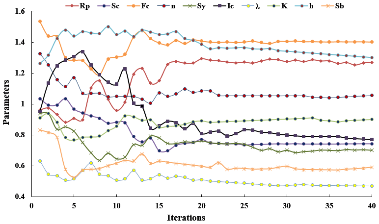
Figure 5 shows that almost all parameters fluctuated widely at the beginning of the optimization. After approximately 15 iterations of optimization calculations, most of the linear fluctuations became significantly less volatile, which indicated that the algorithm was tending towards convergence (possibly only locally). When the number of iterations exceeded 25, all parameters remained essentially unchanged, meaning that the algorithm had converged (at this point, there was global convergence). It took only 25 iterations to reach a definite convergence of the parameter rates with the ICPSO algorithm, which is extremely efficient in terms of the parameter optimization of distributed hydrological models. In previous studies of the parametric optimization for the Karst–Liuxihe model in similar basin areas, 50 automatic parameter optimization iterations were required to reach convergence (Li et al., 2021), demonstrating the effectiveness of the ICPSO algorithm.
To evaluate the effect of parameter optimization, the convergence efficiency of the algorithm and, more importantly, the parameters after calibration were used to simulate floods. Figure 6 shows the flood simulation effects.
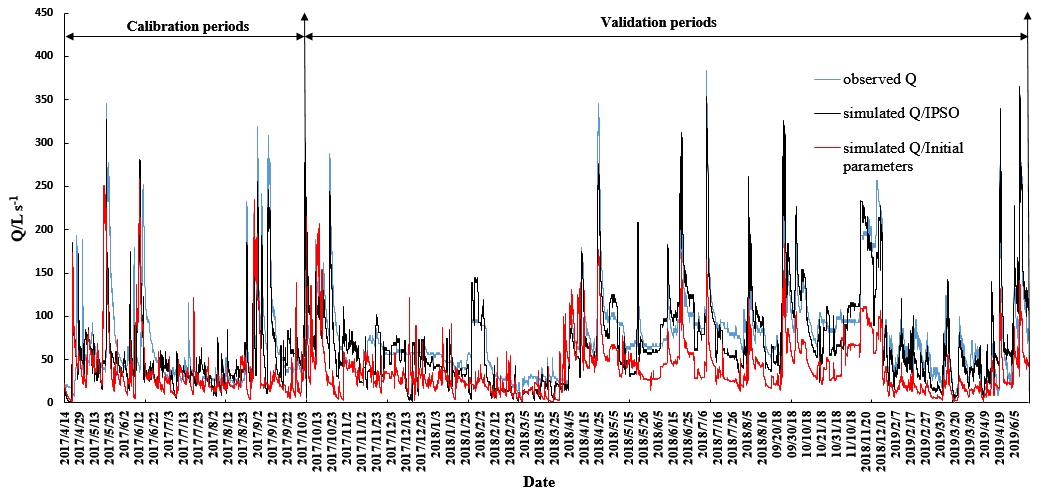
Figure 6 shows that the flows simulated by parameter optimization were better than those simulated by the initial model parameters. The simulated flow processes based on the initial parameters were relatively small, with the simulated peak flows in particular being smaller than the observed values, and there were large errors between the two values. In contrast, the simulated flows produced by the QMG model after parameter optimization were very similar to the observed values, which indicated that calibration of the model parameters was necessary and that there was an improvement in parameter optimization through the use of the ICPSO algorithm in this study. In addition, it was found that the flow simulation effect was better in the calibration periods than in the validation periods (Fig. 6).
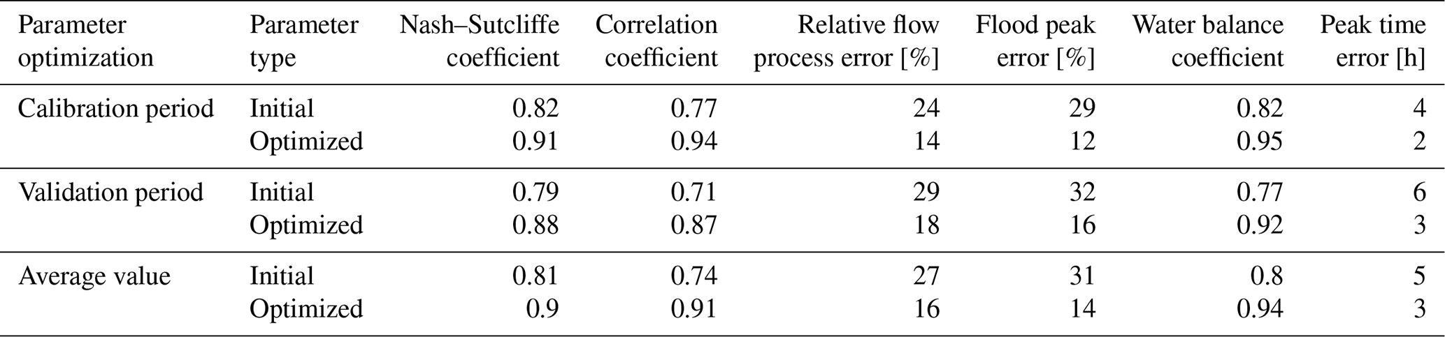
To compare the flow process simulation results based on the initial model parameters with the optimized parameters, six evaluation indices (Nash–Sutcliffe coefficient, correlation coefficient, relative flow process error, flood peak error, water balance coefficient and peak time error) were applied in this study, and the results are presented in Table 3.
Table 3 shows that the evaluation indices of the flood simulations after parametric optimization were better than those of the initial model parameters. The average values of the initial parameters for these six indices were 0.81, 0.74, 27 %, 31 %, 0.80 and 5 h, respectively. For the optimized parameters, the average values were 0.90, 0.91, 16 %, 14 %, 0.94 and 3 h, respectively. The flood simulation effects after parameter optimization were clearly improved, implying that parameter optimization of the QMG model was necessary and that the ICPSO algorithm was an effective approach for parameter optimization that could greatly improve the convergence efficiency of parameter optimization and ensure that the model performed well in flood simulations.
4.3 Model validation
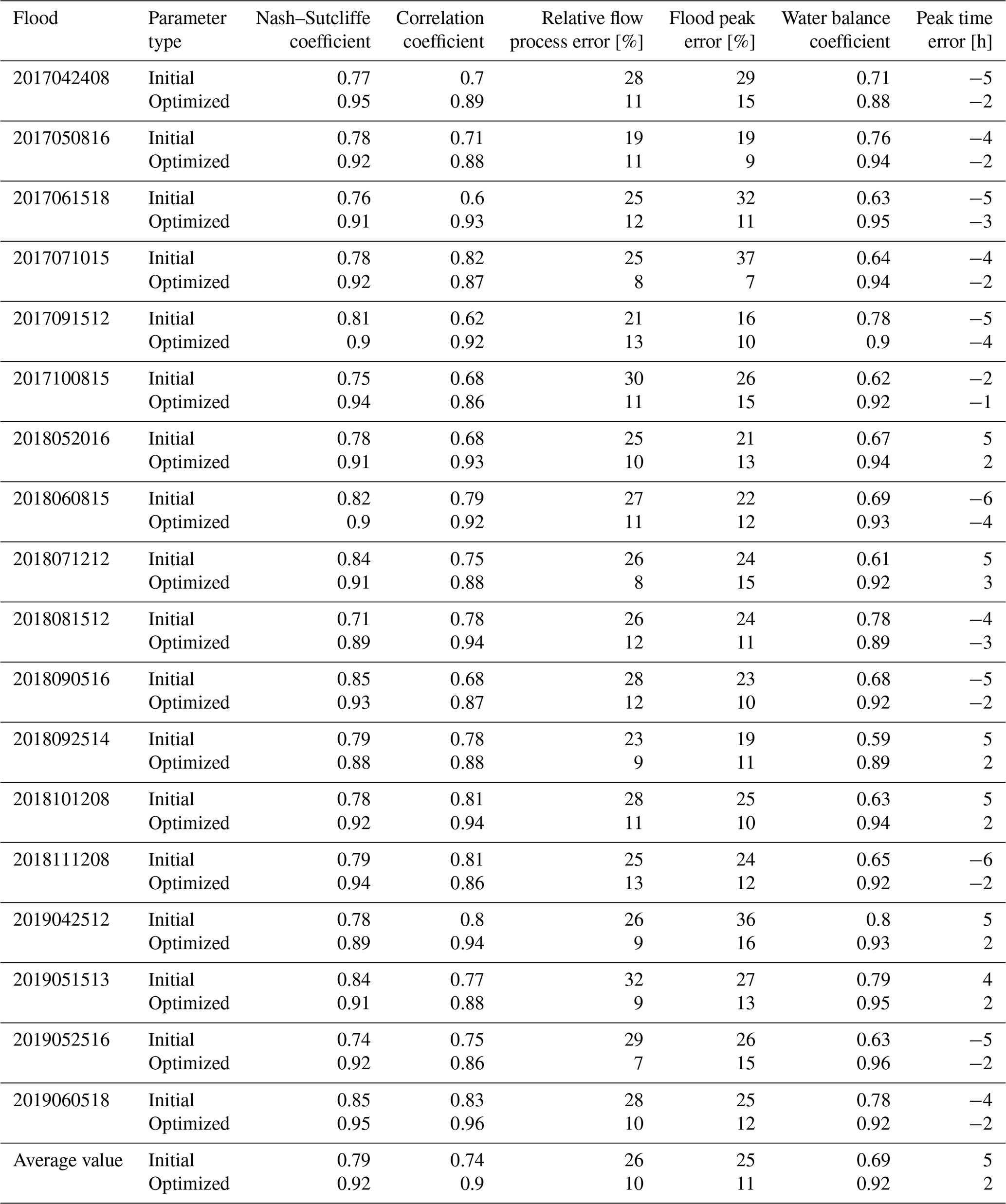
Following parameter optimization, we simulated the whole flow process (14 April 2017 to 10 June 2019) based on the optimized and initial parameters of the QMG model (Fig. 6), which enabled a visual reflection of the application of the model for the simulation of a long series of flow processes. To reflect the simulation effects of the model for different flood events, we divided the whole flow process into 18 flood events and then used the initial parameters of the model and the optimized parameters to verify the model performance in flood simulations. Figure 7 and Table 4 show the flood simulation effects and their evaluation indices obtained using both the initial and the optimized parameters.
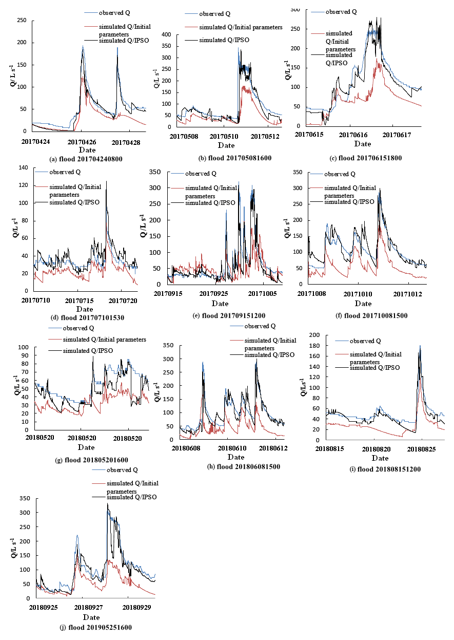
Figure 7 shows that the flood simulation results obtained using the initial parameters were smaller than the observed values and that the model performance in flood simulations improved after parameter optimization. The simulated flood processes were in good agreement with observations and were especially effective for simulating flood peak flows. From the flood simulation indices in Table 4, the average water balance coefficient based on the initial parameters was 0.69, i.e. much less than 1, indicating that the simulated water in the model was unbalanced. After parameter optimization, the average value was 0.92, indicating that parameter optimization had a significant impact on the model water balance calculation.
Table 4 shows that the average values of the six indices (Nash–Sutcliffe coefficient, correlation coefficient, relative flow process error, flood peak error, water balance coefficient and peak time error) for the initial parameters were 0.79, 0.74, 26 %, 25 %, 0.69 and 5 h, respectively, while for the optimized parameters, the average values were 0.92, 0.90, 10 %, 11 %, 0.92 and 2 h, respectively. All evaluation indices improved after parameter optimization, with the average values of the Nash–Sutcliffe coefficient, correlation coefficient and water balance coefficient increasing by 0.13, 0.16 and 0.23, respectively. The average values of the relative flow process error, flood peak error and peak time error decreased by 15 %, 14 % and 3 h, respectively. These reasonable flood simulation results confirmed that parameter optimization by the ICPSO algorithm was necessary and effective for the QMG model.
5.1 Model evaluation
Compared with the overall flow process simulation shown in Fig. 6, each flood process was better simulated by the QMG model (Fig. 7). This was because the main consideration of the QMG model was the calculation of the flood process and the correlation algorithm of the dry season runoff was not sufficiently described. For example, Eqs. (12)–(15) represent the flood convergence algorithm. As a result, the model is not good at simulating other flow processes, such as dry season runoff, leading to a low accuracy in the overall flow process. The next phase of our research will focus on refining the algorithm related to dry season runoff and improving the comprehensive performance of the model.
5.2 Parameter sensitivity analysis
The parameter sensitivity results in Table 2 show that the rainfall infiltration coefficient in the QMG model was the most sensitive parameter. This was the key to determining the generation of excess infiltration surface runoff and separating surface runoff from subsurface runoff. If the rainfall infiltration coefficient was greater than the infiltration capacity, excess infiltration surface runoff was generated on the exposed karst landforms; otherwise, all rainfall would infiltrate to meet the water deficit in the vadose zone and then continue to seep into the underground river system, eventually flowing out of the basin through the underground river outlet. The confluence modes of surface runoff and underground runoff were completely different, resulting in a large difference in the simulated flow results. Therefore, the rainfall infiltration coefficient had the greatest impact on the final flood simulation results.
Other highly sensitive parameters, such as the rock permeability coefficient, rock porosity and specific yield, were used as the basis for dividing between slow flow in karst fissures and rapid flow in conduits. The division of slow and rapid flows also had a great impact on the discharge at the outlet of the basin. Slow flow plays an important role in water storage in a karst aquifer and is very important for the replenishment of river base flow in the dry season. Rapid flow in large conduit systems dominates flood runoff and is the main component of the flood water volume in the flood season.
Parameters related to the soil water content, including the saturated water content, field capacity and thickness, were sensitive parameters and had a strong influence on the flood simulation results. This is because the soil moisture content prior to flooding affects how flood flows rise and when peaks occur. If the soil is already very wet or even saturated before flooding, the flood rises quickly to a peak, and the process line of the flood peak flow is sharp and thin. This type of flood process forms easily and can lead to disaster-causing flood events. In contrast, if the soil in the basin is very dry before flooding, the rainfall first counteracts the water shortage of the vadose zone, and after this zone is replenished, the rainfall infiltrates into the underground river. The flood peak of the river basin outlet is therefore delayed.
The flow direction, slope and soil coefficient were moderately sensitive parameters. They had a specific influence on the flood simulation results, but the influence was not as great as that of the highly sensitive and sensitive parameters. The channel roughness and the evaporation coefficient were insensitive parameters. The amount of water lost by evapotranspiration is a very small in part of the total flood water, and it was therefore the least sensitive parameter in the QMG model.
5.3 Assessment and reduction of uncertainty
In general, the uncertainty in model simulation is due mainly to three aspects of the model: (i) the uncertainty of its input data, (ii) the uncertainty of its structure and algorithm, and (iii) the uncertainty of its parameters. In the practical application of a hydrological model, these three uncertainties are usually interwoven, which leads to the overall uncertainty of the final simulation results (Krzysztofowicz, 2014). Therefore, the present study focused on the uncertainties in the input data, the model structure and the parameters to reduce the overall uncertainty of the simulation results.
First, the input data – mainly rainfall-runoff data and hydrogeological data – were preprocessed, which substantially reduced their uncertainty. Second, we simplified the structure of the QMG model, which is reflected in the fact that it has only two layers of spatial structure in the horizontal and vertical directions. This relatively simple structure greatly reduced the model structure-related uncertainty. In contrast, the underground structure of our previous Karst–Liuxihe model (Li et al., 2021) has five layers, which leads to great uncertainty. Third, appropriate algorithms for runoff generation and confluence were selected. Different models were designed for different purposes, which led to great differences in the algorithms used. In the QMG model, most of the rainfall-runoff algorithms used have been validated against the research results of others, and some of them were improved to suit karst flood simulation and prediction by the QMG model. For example, the algorithm for the generation of excess infiltration runoff (Eq. 2) represented an improvement over the version used in the Liuxihe model (Chen et al., 2010; Li et al., 2020). Finally, the algorithm for parameter optimization was improved. Considering that the standard PSO algorithm tends to converge locally, this study developed the ICPSO for parameter optimization by adding chaotic perturbation factors. The flood simulation results after parameter optimization were much better than those of the initial model parameters (Figs. 6 and 7 and Tables 2 and 3), which indicates that parameter optimization is necessary for a distributed hydrological model and can reduce the uncertainty of the model parameters.
This study proposed a new distributed physically based hydrological model, i.e. the QMG model, to accurately simulate floods in karst trough and valley landforms. The main conclusions of this paper are as follows:
-
The QMG model has a high application potential for karst hydrology simulations. Other distributed hydrological models usually have multiple structures, resulting in the need for a large amount of data to build models in karst areas (Kraller et al., 2014). The QMG model has only a double-layer structure, with a clear physical meaning, and a small amount of basic data is needed to build the model in karst areas, such as some necessary hydrogeological data. For example, the distribution and flow directions of underground rivers are needed, which can be inferred from a tracer test, leading to a low modelling cost. There are fewer parameters in the QMG model than in other distributed hydrological models, with only 10 parameters that need to be calibrated.
-
The flood simulation after parameter optimization was much better than the simulation using the initial model parameters. After parameter optimization, the average values of the Nash–Sutcliffe coefficient, correlation coefficient and water balance coefficient increased by 0.13, 0.16 and 0.23, respectively, while the average relative flow process error, flood peak error and peak time error decreased by 15 %, 14 % and 3 h, respectively. Parameter optimization is necessary for a distributed hydrological model, and the improvement of the ICPSO algorithm in this study was an effective way to achieve this.
-
In the QMG model, the rainfall infiltration coefficient Ic, rock permeability coefficient K, rock porosity Rp and the parameters related to the soil water content were sensitive parameters. The order of the parameter sensitivity values was as follows: infiltration coefficient > permeability coefficient > rock porosity > specific yield > saturated water content > field capacity > flow direction > thickness > slope > soil coefficient > channel roughness > evaporation coefficient.
The QMG model is suitable for karst trough and valley landforms such as the current study area, where the topography is conducive to the spread of flood water. Whether this model is applicable to the karst areas of other landforms still needs to be verified in future studies. In addition, the basin area is very small, while the hydrological similarity between different small basin areas varies greatly (Kong and Rui, 2003). The size of the area to be modelled has a great influence on the choice of model spatial resolution (Chen et al., 2017). Therefore, whether the QMG model is suitable for flood prediction in large karst basins needs to be determined.
Model development
The QMG model presented in this study uses Visual Basic language programming. The general framework of the model and the algorithm consist of three parts: the modelling approach, the algorithm of rainfall-runoff generation and confluence, and the parameter optimization algorithm. As this model is a free and open-source hydrological modelling programme (QMG model-V1.0), we provide all modelling packages, including the model code, installation package, simulation data package and user manual, free of charge. It is important to note that the model we provide is only for scientific research purposes and should not be used for any commercial purposes. Creative Commons Attribution 4.0 International.
The model installation programme can be downloaded from ZENODO; cite as Li (2021a) and Li (2021b) (registration required). The user manual can be downloaded from https://doi.org/10.5281/zenodo.4964754 (Li, 2021c).
All codes for the QMG model-V1.0 in this paper are available for free, and the code can be downloaded from ZENODO (https://doi.org/10.5281/zenodo.4964709; Li, 2021d) (registration required).
All data used in this paper are available, findable, accessible, interoperable and reusable. The simulation data and modelling data package (including the DEM data, land use type and soil type data) can be downloaded from https://doi.org/10.5281/zenodo.4964727 (Li, 2021e).
JLi was responsible for the calculations and writing of the whole paper. DY helped conceive the structure of the model. FZ and JLiu provided significant assistance in the English translation of the paper. MM provided flow data for the study area.
The contact author has declared that none of the authors has any competing interests.
Publisher's note: Copernicus Publications remains neutral with regard to jurisdictional claims in published maps and institutional affiliations.
The authors thank various financial supporters (detailed below) that provided funding for this study. The authors also thank multiple reviewers and editors for their comments on the manuscript, which greatly improved the quality of this paper. Special thanks to Fuxi Zhang, and Jiao Liu for their help in revising the language and writing.
This study was supported by the National Natural Science Foundation of China (grant no. 41830648), the National Science Foundation for Young Scientists of China (grant no. 42101031), the Fundamental Research Funds for the Central Universities (grant no. SWU-KQ22001), the Chongqing Natural Science Foundation (grant no. cstc2021jcyj-msxm0007), and the Chongqing Education Commission Science and Technology Research Foundation (grant no. KJQN202100201), Drought Monitoring, Analysing and Early Warning of Typical Prone-to-Drought Areas of Chongqing (grant no. 20C00183), and the Open Project Program of Guangxi Key Science and Technology Innovation Base on Karst Dynamics (grant nos. KDL & Guangxi 202009 and KDL & Guangxi 202012).
This paper was edited by Bethanna Jackson and reviewed by four anonymous referees.
Abbott, M. B., Bathurst, J. C., Cunge, J. A., O'Connell, P. E., and Rasmussen, J.: An Introduction to the European HydrologicSystem-System Hydrologue Europeen, `SHE', a: History and Philosophy of a Physically-based, Distributed Modelling System, J. Hydrol., 87, 45–59, 1986a.
Abbott, M. B., Bathurst, J. C., Cunge, J. A., O'Connell, P. E., and Rasmussen, J.: An Introduction to the European Hydrologic System-System Hydrologue Europeen, `SHE', b: Structure of a Physically based, distributed modeling System, J. Hydrol., 87, 61–77, 1986b.
Ambroise, B., Beven, K., and Freer, J.: Toward a generalization of the TOPMODEL concepts: Topographic indices of hydrologic similarity, Water Resour. Res., 32, 2135–2145, 1996.
Atkinson, T. C.: Diffuse flow and conduit flow in limestone terrain in the Mendip Hills, Somerset (Great Britain), J. Hydrol., 35, 93–110, https://doi.org/10.1016/0022-1694(77)90079-8, 1977.
Berry, R. A., Saurel, R., and Lemetayer, O.: The discrete equation method (DEM) for fully compressible, two-phase flows in ducts of spatially varying cross-section, Nucl. Eng. Design, 240, 3797–3818, 2010.
Beven, K., and Binley, A.: The future of distributed models: Model calibration and uncertainty prediction, Hydrol. Process., 6, 279–298, 2006.
Birk, S., Geyer, T., Liedl, R., and Sauter, M.: Process-based interpretation of tracer tests in carbonate aquifers, Ground Water, 43, 381–388, 2005.
Bittner, D., Parente, M. T., Mattis, S., Wohlmuth, B., and Chiogna, G.: Identifying relevant hydrological and catchment properties in active subspaces: An inference study of a lumped karst aquifer model, Adv. Water Resour., 135, 550–560, https://doi.org/10.1016/j.advwatres.2019.103472, 2020.
Blansett, K. L.: Flow, water quality, and SWMM model analysis for five urban karst basins, PhD thesis, The Pennsylvania State University, USA, https://www.doc88.com/p-0753138375298.html (last access: 29 March 2016), 2011.
Blansett, K. L. and Hamlett, J. M.: Challenges of Stormwater Modeling for Urbanized Karst Basins. Pittsburgh, Pennsylvania, an ASABE Meeting Presentation, Paper Number 1009274, https://doi.org/10.13031/2013.29840, 2010.
Bonacci, O., Ljubenkov, I., and Roje-Bonacci, T.: Karst flash floods: an example from the Dinaric karst (Croatia), Nat. Hazards Earth Syst. Sci., 6, 195–203, https://doi.org/10.5194/nhess-6-195-2006, 2006.
Chang, Y. and Liu, L.: A review of hydrological models in karst areas, Engineering investigation, 43, 37–44, 2015.
Chang, Y., Hartmann, A., Liu, L., Jiang, G., and Wu, J.: Identifying more realistic model structures by electrical conductivity observations of the karst spring, Water Resour. Res., 57, e28587, https://doi.org/10.1029/2020WR028587, 2021.
Chen, Y.: Distributed Hydrological Models. Springer Berlin Heidelberg, Berlin, Germany, https://doi.org/10.1007/978-3-642-40457-3_23-1, 2018.
Chen, Y. B., Ren, Q. W., Huang, F. H., Xu, H. J., and Cluckie, I.: Liuxihe model and its modeling to river basin flood, J. Hydrol. Eng., 16, 33–50, https://doi.org/10.1061/(ASCE)HE.1943-5584.0000286, 2010.
Chen, Y., Li, J., Wang, H., Qin, J., and Dong, L.: Large-watershed flood forecasting with high-resolution distributed hydrological model, Hydrol. Earth Syst. Sci., 21, 735–749, https://doi.org/10.5194/hess-21-735-2017, 2017.
Dewandel, B., Lachassagne, P., Bakalowicz, M., Weng, P., and Malki, A. A.: Evaluation of aquifer thickness by analysing recession hydrographs. Application to the Oman ophiolite hard-rock aquifer, J. Hydrol., 274, 248–269, 2003.
Doummar, J., Sauter, M., and Geyer, T.: Simulation of flow processes in a large scale karst system with an integrated catchment model (MIKE SHE) – identification of relevant parameters influencing spring discharge, J. Hydrol., 426–427, 112–123, 2012.
Epting, J., Page, R. M., and Auckenthaler, A.: Process-based monitoring and modeling of Karst springs – Linking intrinsic to specific vulnerability, Sci. Total Environ., 625, 403–415, 2018.
Fleury, P., Plagnes, V., and Bakalowicz, M.: Modelling of the functioning of karst aquifers with a reservoir model: Application to Fontaine de Vaucluse (South of France), J. Hydrol., 345, 38–49, https://doi.org/10.1016/j.jhydrol.2007.07.014, 2007b.
Gang, L., Tong, F. G., and Bin, T.: A Finite Element Model for Simulating Surface Runoff and Unsaturated Seepage Flow in the Shallow Subsurface, Hydrol. Process., 6, 102–120, https://doi.org/10.1002/hyp.13564, 2019.
Gautama, R. S., Notosiswoyo, S., Zen, M. T., and Kusumayudha, S. B.: Mathematical model of fractal conduits flow mechanics in the gunungsewu karst area, yogyakarta special region, indonesia, Int. J. Hydrol. Sci. Technol., 1, 1, https://doi.org/10.1504/IJHST.2021.10035255, 2021.
Geyer, T., Birk, S., Liedl, R., and Sauter, M.: Quantification of temporal distribution of recharge in karst systems from spring hydrographs, J. Hydrol., 348, 452–463, 2008.
Gou, P. F., Jiang, Y. J., Hu, Z. Y., Pu, J. B., and Yang, P. H.: A study of the variations in hydrology and hydrochemistry under the condition of a storm in a typical karst subterranean stream, Hydrogeol. Eng. Geol., 37, 20–25, 2010.
Guila, J. F., Samper, J., Belén, B., Paloma, G., and Montenegro, L.: Reactive transport model of gypsum karstification in physically and chemically heterogeneous fractured media, Energies, 15, 1–29, 2022.
Gutierrez, F.: Hazards associated with karst, in: Geomorphological Hazards and Disaster Prevention, edited by: Alcantara, I. and Goudie, A., Cambridge University Press, Cambridge, 161–175, 2010.
Gutierrez, F., Parise, M., D' Waele, J., and Jourde, H.: A review on natural and human-induced geohazards and impacts in karst, Earth Sci. Rev., 138, 61–88, 2014.
Hartmann, A.: Experiences in calibrating and evaluating lumped karst hydrological models, Geological Society, London, Special Publications, 466, 331–340, https://doi.org/10.1144/sp466.18, 2018.
Hartmann, A. and Baker, A.: Progress in the hydrologic simulation of time variant of karst systems-Exemplified at a karst spring in Southern Spain, Adv. Water Resour., 54, 149–160, 2013.
Hartmann, A. and Baker, A.: Modelling karst vadose zone hydrology and its relevance for paleoclimate reconstruction, Earth-Sci. Rev., 172, 178–192, 2017.
Hartmann, A., Goldscheider, N., Wagener, T., Lange, J., and Weiler, M.: Karst water resources in a changing world: Review of hydrological modeling approaches, Rev. Geophys., 52, 218–242, https://doi.org/10.1002/2013RG000443, 2014.
Jamal, M. S. and Awotunde, A. A.: Darcy model with optimized permeability distribution (dmopd) approach for simulating two-phase flow in karst reservoirs, J. Petrol. Explor. Prod. Technol., 12, 191–205, https://doi.org/10.1007/S13202-021-01385-X, 2022.
Jourde, H., Roesch, A., Guinot, V., and Bailly-Comte, V.: Dynamics and contribution of karst groundwater to surface flow during Mediterranean flood, Environ. Geol. 51, 725–730, 2007.
Jourde, H., Lafare, A., Mazzilli, N., Belaud, G., Neppel, L., Doerfliger, N., and Cernesson, F.: Flash flood mitigation as a positive consequence of anthropogenic forcings on the groundwater resource in a karst catchment, Environ. Earth Sci., 71, 573–583, 2014.
Jukić, D. and Denić-Jukić, V.: Groundwater balance estimation in karst by using a conceptual rainfall–runoff model, J. Hydrol., 373, 302–315, https://doi.org/10.1016/j.jhydrol.2009.04.035, 2009.
Kong, F. Z. and Rui, X. F.: Hydrological similarity of catchments based on topography, Geogr. Res., 6, 709–715, 2003.
Kovács, A. and Perrochet, P.: A quantitative approach to spring hydrograph decomposition, J. Hydrol., 352, 16–29, https://doi.org/10.1016/j.jhydrol.2007.12.009, 2008.
Kovács, A. and Sauter, M.: Modelling karst hydrodynamics, Frontiers of Karst Research, 26, 13–26, 2008.
Kraller, G., Warscher, M., Strasser, U., Kunstmann, H., and Franz, H.: Distributed hydrological modeling and model adaption in high alpine karst at regional scale (berchtesgaden alps, germany), Springer International Publishing Switzerland, https://doi.org/10.1007/978-3-319-06139-9_8, 2014.
Krzysztofowicz, R.: Probabilistic flood forecast: Exact and approximate predictive distributions, J. Hydrol., 517, 643–651, 2014.
Krzysztofowicz, R. and Kelly, K.: Hydrologic uncertainty processor for probabilistic river stage forecasting, Water Resour. Res., 36, 3265–3277, 2000.
Kurtulus, B. and Razack, M.: Evaluation of the ability of an artificial neural network model to simulate the input-output responses of a large karstic aquifer: the la rochefoucauld aquifer (charente, france), Hydrogeol. J., 15, 241–254, 2007.
Ladouche, B., Marechal, J. C., and Dorfliger, N.: Semi-distributed lumped model of a karst system under active management, J. Hydrol., 509, 215–230, 2014.
Li, J.: QMG model-V1.0, Zenodo, https://doi.org/10.5281/zenodo.4964701, 2021a.
Li, J.: dotNetFx40_Full_x86_x64, Zenodo, https://doi.org/10.5281/zenodo.4964697, 2021b.
Li, J.: User guide for QMG model-VI.0, Zenodo, https://doi.org/10.5281/zenodo.4964754, 2021c.
Li, J.: QMG model-V1.0 code (v1.0), Zenodo [code], https://doi.org/10.5281/zenodo.4964709, 2021d.
Li, J.: Simulated data and modelling data package includes the DEM data, land use type and soil type data, Zenodo [data set], https://doi.org/10.5281/zenodo.4964727, 2021e.
Li, J., Yuan, D., Liu, J., Jiang, Y., Chen, Y., Hsu, K. L., and Sorooshian, S.: Predicting floods in a large karst river basin by coupling PERSIANN-CCS QPEs with a physically based distributed hydrological model, Hydrol. Earth Syst. Sci., 23, 1505–1532, https://doi.org/10.5194/hess-23-1505-2019, 2019.
Li, J., Hong, A., Yuan, D., Jiang, Y., Deng, S., Cao, C., and Liu, J.: A new distributed karst-tunnel hydrological model and tunnel hydrological effect simulations, J. Hydrol., 593, 125639, https://doi.org/10.1016/j.jhydrol.2020.125639, 2020.
Li, J., Hong, A., Yuan, D., Jiang, Y., Zhang, Y., Deng, S., Cao, C., Liu, J., and Chen, Y.: Elaborate Simulations and Forecasting of the Effects of Urbanization on Karst Flood Events Using the Improved Karst-Liuxihe Model, CATENA, 197, 104990, https://doi.org/10.1016/j.catena.2020.104990, 2021.
Liedl, R., Sauter, M., Huckinghaus, D., Clemens, T., and Teutsch, G.: Simulation of the development of karst aquifers using a coupled continuum pipe flow model, Water Resour. Res., 39, 50–57, 2003.
Liu, X., Jiang, Y. J., Ye, M. Y., Yang, P. H., Hu, Z. Y., and Li, Y. Q.: Study on hydrologic regime of underground river in typical karst valley – A case study on the Qingmuguan subterranean stream in Chongqing, Carsologica Sinica, 28, 149–154, 2009.
Lu, D. B., Shi, Z. T., Gu, S. X., and Zeng, J. J.: Application of Hydrological Model in the Karst Area, Water-saving irrigation, 11, 31–34, 2013.
Martinotti, M. E., Pisano, L., Marchesini, I., Rossi, M., Peruccacci, S., Brunetti, M. T., Melillo, M., Amoruso, G., Loiacono, P., Vennari, C., Vessia, G., Trabace, M., Parise, M., and Guzzetti, F.: Landslides, floods and sinkholes in a karst environment: the 1–6 September 2014 Gargano event, southern Italy, Nat. Hazards Earth Syst. Sci., 17, 467–480, https://doi.org/10.5194/nhess-17-467-2017, 2017.
Masciopinto, C., Passarella, G., Caputo, M. C., Masciale, R., and Carlo, L. D.: Hydrogeological models of water flow and pollutant transport in karstic and fractured reservoirs, Water Resour. Res., 57, https://doi.org/10.1029/2021WR029969, 2021.
Meng, H. H. and Wang, N. C.: Advances in the study of hydrological models in karst basin, Prog. Geogr., 29, 1311–1318, 2010.
Meng, H. H., Wang, N. C., Su, W. C., and Huo, Y.: Modeling and application of karst semi-distributed hydrological model based on sinkholes, Scientia Geographica Sinica, 5, 550–554, https://doi.org/10.3969/j.issn.1000-0690.2009.04.014, 2009.
Pan, H. Y.: Hydrological model and application in karst watersheds, China University of Geosciences, PhD thesis, Wuhan, China, 2014.
Parise, M.: Hazards in karst, Proceedings Int. Conf. “Sustainability of the karst environment. Dinaric karst and other karst regions”, IHP-Unesco, Series on Groundwater, 2, 155–162, 2010.
Peterson, E. W. and Wicks, C. M.: Assessing the importance of conduit geometry and physical parameters in karst systems using the storm water management model (SWMM), J. Hydrol., 329, 294–305, 2006.
Peterson, J. R. and Hamlett, J. M.: Hydrologic calibration of the SWAT model in a basin containing fragipan soils, J. Am. Water Resour. As., 34, tb00952.x, https://doi.org/10.1111/j.1752-1688.1998, 1998.
Petrie, R., Denvil, S., Ames, S., Levavasseur, G., Fiore, S., Allen, C., Antonio, F., Berger, K., Bretonnière, P.-A., Cinquini, L., Dart, E., Dwarakanath, P., Druken, K., Evans, B., Franchistéguy, L., Gardoll, S., Gerbier, E., Greenslade, M., Hassell, D., Iwi, A., Juckes, M., Kindermann, S., Lacinski, L., Mirto, M., Nasser, A. B., Nassisi, P., Nienhouse, E., Nikonov, S., Nuzzo, A., Richards, C., Ridzwan, S., Rixen, M., Serradell, K., Snow, K., Stephens, A., Stockhause, M., Vahlenkamp, H., and Wagner, R.: Coordinating an operational data distribution network for CMIP6 data, Geosci. Model Dev., 14, 629–644, https://doi.org/10.5194/gmd-14-629-2021, 2021.
Qin, J. G. and Jiang, Y.P.: A review of numerical simulation methods for CFP pipeline flow, Groundwater, 3, 98–100, 2014.
Reimann, T. and Hill, M. E.: Modflow-cfp: a new conduit flow process for modflow–2005, Ground Water, 47, 321–325, https://doi.org/10.1111/j.1745-6584.2009.00561.x, 2009.
Shoemaker, W. B., Cunningham, K. J., and Kuniansky, E. L.: Effects of turbulence on hydraulic heads and parameter sensitivities in preferential groundwater flow layers, Water Resour. Res., 44, 34–50, https://doi.org/10.1029/2007WR006601, 2008.
Suo, L. T., Wan, J. W., and Lu, X. W.: Improvement and application of TOPMODEL in karst region, Carsologica Sinica, 26, 67–70, 2007.
Teixeiraparente, M., Bittner, D., Mattis, S. A., Chiogna, G., and Wohlmuth, B.: Bayesian calibration and sensitivity analysis for a karst aquifer model using active subspaces, Water Resour. Res., 55, 342–356, https://doi.org/10.1029/2019WR024739, 2019.
White, W. B.: Karst hydrology: recent developments and open questions, Eng. Geol., 65, 85–105, 2002.
Williams, P. W.: The role of the epikarst in karst and cave hydrogeology: a review, Int. J. Speleol., 37, 1–10, 2008.
Williams, P. W.: Book Review: Methods in Karst Hydrogeology, Goldscheider, N. and Drew, D., Hydrogeol. J., 17, 1025–1025, 2009.
Yang, P. H., Luo, J. Y., Peng, W., Xia, K. S., and Lin, Y. S.: Application of online technique in tracer test-A case in Qingmuguan subterranean river system, Chongqing, China, Carsologica Sinica, 27, 215–220, 2008.
Yu, D., Yin, J., Wilby, R. L., Stuart, N. L., Jeroen, C., Lin, N., Liu, M., Yuan, H., Chen, J., Christel, P., Guan, M., Avinoam, B., Charlie, W. D., Tang, X., Yu, L., and Xu, S.: Disruption of emergency response to vulnerable populations during floods, Nat. Sustain., 3, 728–736, https://doi.org/10.1038/s41893-020-0516-7, 2020.
Yu, Q., Yang., P. H., Yu, Z. L., Chen, X. B., and Wu, H.: Dominant factors controlling hydrochemical variationg of karst underground river in different period, Qingmuguan, Chongqing, Carsologica Sinica, 35, 134–143, 2016.
Zhang, H.: Characterization of a multi-layer karst aquifer through analysis of tidal fluctuation, J. Hydrol., 601, 126677, https://doi.org/10.1016/j.jhydrol.2021.126677, 2021.
Zhang, Q.: Assesment on the intrinsic vulnerability of karst groundwater source in the Qingmuguan karst valley, Carsologica Sinica, 31, 67–73, 2012.
Zhu, C. and Li, Y.: Long-Term Hydrological Impacts of Land Use/Land Cover Change From 1984 to 2010 in the Little River Basin, Tennessee, International Soil and Water Conservation Research, 2, 11–21, 2014.