Parallel implementation of the SHYFEM (System of HydrodYnamic Finite Element Modules) model

This paper presents the message passing interface (MPI)-based parallelization of the three-dimensional hydrodynamic model SHYFEM (System of HydrodYnamic Finite Element Modules). The original sequential version of the code was parallelized in order to reduce the execution time of high-resolution configurations using state-of-the-art high-performance computing (HPC) systems. A distributed memory approach was used, based on the MPI. Optimized numerical libraries were used to partition the unstructured grid (with a focus on load balancing) and to solve the sparse linear system of equations in parallel in the case of semi-to-fully implicit time stepping. The parallel implementation of the model was validated by comparing the outputs with those obtained from the sequential version. The performance assessment demonstrates a good level of scalability with a realistic configuration used as benchmark.

1 Introduction

Ocean sciences are significantly supported by numerical modeling, which helps to understand physical phenomena or provide predictions both in the short term or from a climate perspective. The reliability of ocean prediction is strictly linked to the ability of numerical models to capture the relevant physical processes.

The physical processes taking place in the oceans occupy a wide range of spatial and timescales. The ocean circulation is highly complex, in which physical processes at large scales are transferred to smaller scales, resulting in mesoscale and sub-mesoscale structures, or eddies (Hallberg, 2013).

The coastal scale is also rich in features driven by the interaction between the regional-scale dynamics and the complex morphology typical of shelf areas, tidal flats, estuaries and straits.

In both large-scale and coastal modeling, the spatial resolution is a key factor.

Large-scale applications require a finer horizontal resolution than the Rossby radius (in the order of 100 km in midlatitudes and less than 10 km in high latitudes) to capture the mesoscale (Maltrud and McClean, 2005). The geometry of the domain drives the selection of spatial resolution in the coastal environment, where grid spacing can be in the order of meters.

Ocean circulation models use mostly structured meshes and have a long history of development (Griffies et al., 2010) often organized in a community model framework.

In the last few decades, however, the finite-volume (Casulli and Walters, 2000; Chen et al., 2003) or the finite-element approach (Danilov et al., 2004; Zhang et al., 2016; Umgiesser et al., 2004), applied to unstructured meshes, has become more common, especially in the coastal framework, where the flexibility of the mesh particularly suits the complexity of the environment. Applications of unstructured grids include the modeling of storm surges (Westerink et al., 2008), ecosystem modeling (Zhang et al., 2020), sediment transport (Stanev et al., 2019) and flow exchange through straits (Stanev et al., 2018).

Representing several spatial scales in the same application renders the unstructured grid appealing in simulations aimed at bridging the gap between the large-scale flow and the coastal dynamics (Ringler et al., 2013). Advances in the numerical formulation have meant that unstructured models can also be used for large-scale simulations that address geostrophic adjustments and conservation properties comparably to regular grids (Griffies et al., 2010), thus leading to simulations that are suitable for climate studies (Danilov et al., 2017; Petersen et al., 2019).

The computational cost of a numerical simulation depends on the order of accuracy of the numerical scheme and the grid scale (Sanderson, 1998). In the case of structured grids, the computational cost increases inversely on the grid space with the power of the dimensions represented by the model. Estimating the computational cost in unstructured grids is not as straightforward as in regular grids, but it is commensurate to the latter when low-order schemes are used (Ringler et al., 2013; Koldunov et al., 2019).

Both large-scale and coastal applications may involve significant computational resources because of the high density of mesh descriptor elements required to resolve dominant physical processes. The computational cost is also determined by upper limits on the time step, making meaningful simulations prohibitive for conventional machines. Access to HPC resources is essential for performing state-of-the-art simulations.

Several successful modeling studies have involved the SHYFEM (System of HydrodYnamic Finite Element Modules) unstructured grid model (Umgiesser et al., 2004; Bellafiore and Umgiesser, 2010) in the development of regional (Ferrarin et al., 2019; Bajo et al., 2014; Ferrarin et al., 2018) and coastal applications (Umgiesser et al., 2014).

The range of applications of SHYFEM was recently extended in a multi-model study to assess the hazards related to climate scenarios (Torresan et al., 2019), the change in sea level in tidal marshes in response to hurricanes (Park et al., 2022), and in a high-resolution simulation of the Turkish Strait System dynamics under realistic atmospheric and lateral forcing (Ilicak et al., 2021).

SHYFEM was also applied to produce seamless three-dimensional hydrodynamic short-term forecasts on a daily basis (Federico et al., 2017; Ferrarin et al., 2019) from large to coastal scales. SHYFEM has also been used in relocatable mode (Trotta et al., 2021) to support emergency responses to extreme events and natural hazards in the world's oceans. Both in forecasting systems and relocatable services, the need for reduced computational costs is crucial in order to deliver updated forecasts with a longer time window.

We implemented a version of the SHYFEM code that can be executed on parallel architectures, addressing the problem of load balancing that is strictly related to the grid partitioning, the parallel scalability and inter-node computational overhead. Our aim was to make all these applications (study process simulation at different scales, long-term and climatic implementations, forecasting and relocatable systems) practical, also from a future perspective where the computational cost is constantly increasing with the complexity of the simulations. We adopted a distributed memory approach, with two key advantages: (i) reduction in runtime with the upper limit determined by the user's choice of resources and (ii) memory scalability, allowing for highly memory-demanding simulations.

The distributed memory approach, based on the message passing interface (MPI) (The MPI Forum, 1993), can coexist with the shared memory approach and is widely used to parallelize unstructured ocean models, such as MPAS (Ringler et al., 2013) and FESOM2 (Danilov et al., 2017), which are devised for global configurations. MPI codes that address coastal processes include SLIM3D (Kärnä et al., 2013), SCHISM (Zhang et al., 2016) and FVCOM (Chen et al., 2003; Cowles, 2008).

The MPI developments carried out in this work consist of additional routines that wrap the native MPI directives, without undermining the code readability. Some aspects of the parallel development, such as the domain decomposition and the solution of free surface equations, were achieved using external libraries.

Section 2 introduces the SHYFEM model and its main features. Section 3 describes the methodology and the design of the distributed memory parallelization, through the partitioning strategy and management of the data dependencies among the MPI processes. Section 4 describes the implementation; Sect. 5 presents the model validation and the performance assessment. Finally, the conclusions are drawn in the last section.

2 The SHYFEM model

SHYFEM solves the ocean primitive equations, assuming incompressibility in the continuity equation, and advection–diffusion equation for active tracers using finite-element discretization based on triangular elements (Umgiesser et al., 2004). The model uses a semi-implicit algorithm for the time integration of the free surface equation, which makes the solution stable by damping the fastest external gravity waves. The Coriolis term and pressure gradient in the momentum equation and the divergence terms in the continuity equation are treated semi-implicitly. The vertical eddy viscosity and vertical eddy diffusivity in the tracer equations are treated fully implicitly for stability reasons. The advective and horizontal diffusive terms in the momentum and tracer equations are treated explicitly. Smagorinsky's formulation (Blumberg and Mellor, 1987; Smagorinsky, 1963) is used to parameterize the horizontal eddy viscosity and diffusivity. To compute the vertical viscosities, a turbulence closure scheme was used. This scheme is adapted from the k–epsilon​​​​​​​ module of GOTM (General Ocean Turbulence Model) described in (Burchard and Petersen, 1999). A detailed description of the 3D model equations is given in Bellafiore and Umgiesser (2010); Maicu et al. (2021).

Table 1 Notations adopted in this work.

n/a: not applicable.

2.1 Time discretization

SHYFEM equations are discretized in time with a forward time stepping scheme with terms that are evaluated at time level n+1 with weight $\mathrm{0}\le \mathit{\theta }\le \mathrm{1}$ and terms evaluated at time level n with weight 1−θ. The time level n+1 of external pressure gradient in the momentum equations has a weight $\mathit{\gamma }\in [\mathrm{0},\mathrm{1}]$ and the time level of the divergence of barotropic flow in the continuity equation has a weight $\mathit{\beta }\in [\mathrm{0},\mathrm{1}]$. When one of γ or β is 0, the scheme is considered explicit in time.

The treatment of external pressure gradient and divergence in continuity is consistent with the method described in Campin et al. (2004) and used in the pressure method of MITgcm (Marshall et al., 1997).

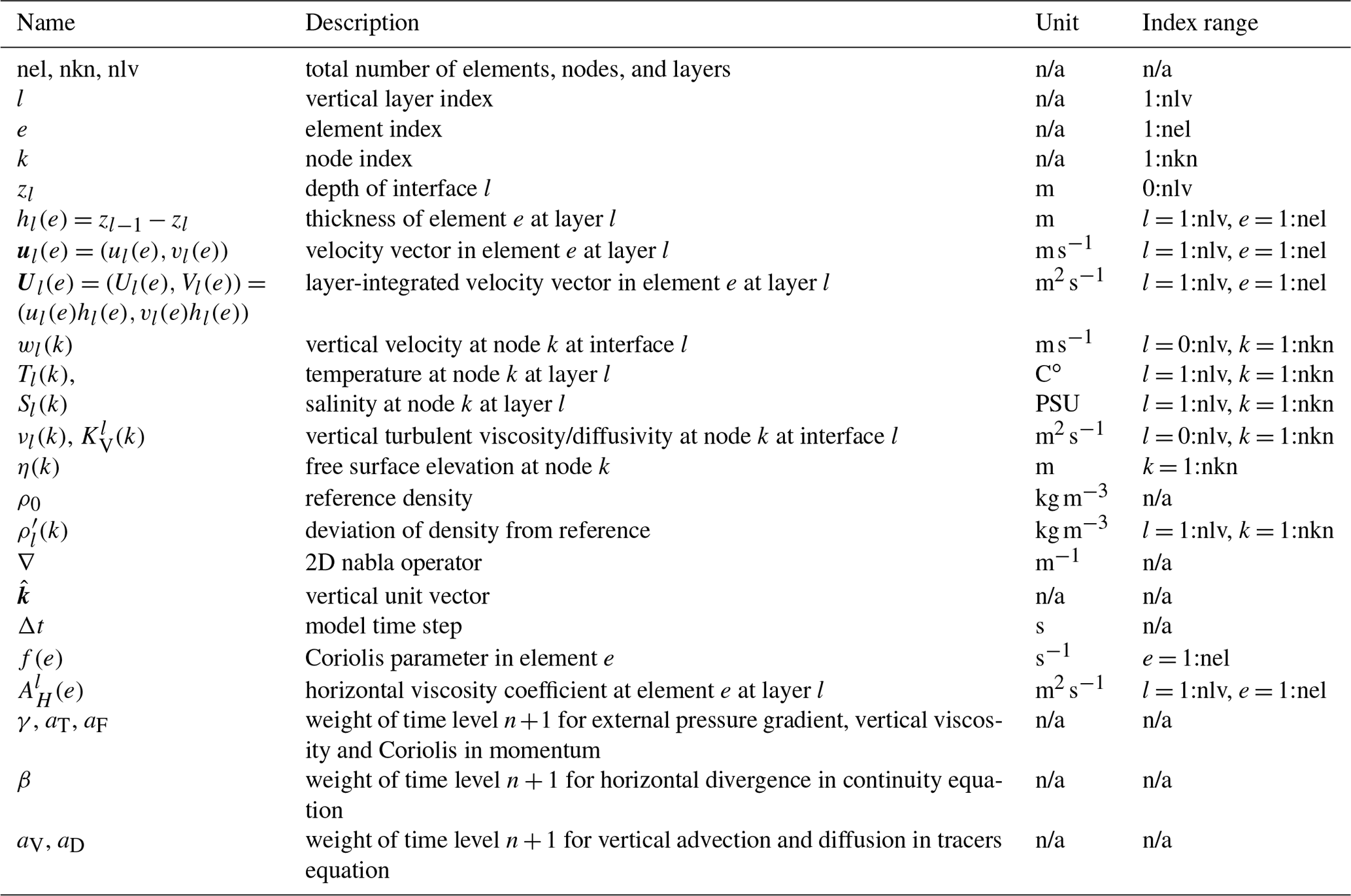
SHYFEM applies a semi-implicit scheme to the Coriolis force and vertical viscosity with weights of time level n+1 a_F and a_T, respectively. As described in (Campin et al., 2004), the solution requires a time step for the momentum from time level n to the intermediate level ^∗. Using the notation reported in Table 1, the velocity equation integrated over a generic layer l is

$$\begin{array}{}\text{(1)}& \begin{array}{rl}& \left({\displaystyle \frac{{\mathit{U}}_l^{\ast }-{\mathit{U}}_l^n}{\mathrm{\Delta }t}}\right)+a_{\mathrm{F}}\mathrm{\Delta }tf\widehat{\mathit{k}}\times \left({\displaystyle \frac{{\mathit{U}}_l^{\ast }-{\mathit{U}}_l^n}{\mathrm{\Delta }t}}\right)\\ & -a_{\mathrm{T}}\mathrm{\Delta }t{D}_z\left({\displaystyle \frac{{\mathit{U}}_l^{\ast }-{\mathit{U}}_l^n}{\mathrm{\Delta }t}}\right)\\ & ={\mathit{F}}_l^n-f\widehat{\mathit{k}}\times {\mathit{U}}_l^n+D_z{\mathit{U}}_l^n-g{h}_l^n\mathbf{\nabla }{\mathit{\eta }}^n,\end{array}\end{array}$$

where D_z is the vertical viscosity operator and the term ${\mathit{F}}_l^n$ contains advection, horizontal turbulent viscosity and pressure terms:

$$\begin{array}{}\text{(2)}& \begin{array}{rl}{\mathit{F}}_l^n=& \left({\mathit{u}}_l^n\mathrm{\nabla }\right){\mathit{U}}_l^n+\underset{z_l}{\overset{z_{l-\mathrm{1}}}{\int }}{w}^n{\displaystyle \frac{\partial {\mathit{u}}^n}{\partial z}}\mathrm{d}z+A_H^l{\mathrm{\nabla }}^{\mathrm{2}}{\mathit{U}}_l^n\\ & +{\displaystyle \frac{h_l}{{\mathit{\rho }}_{\mathrm{0}}}}\mathrm{\nabla }{p}_{\text{atm}}+{\displaystyle \frac{g{h}_l}{{\mathit{\rho }}_{\mathrm{0}}}}\underset{z_{l-\mathrm{1}/\mathrm{2}}}{\overset{{\mathit{\eta }}^n}{\int }}\mathrm{\nabla }{\mathit{\rho }}^{\prime }\mathrm{d}z.\end{array}\end{array}$$

The implementation of D_z is given in Appendix B. The vertical viscosity in the momentum equation is commonly treated implicitly in numerical ocean models. This is because the inversion of the tri-diagonal matrix associated with the system is not computationally demanding.

SHYFEM considers the semi-implicit treatment of the Coriolis term, since it can lead to instability when the friction is too low. The weights assigned to time level n and n+1 of this term in the ocean models that perform semi-implicit treatment are commonly $\mathrm{0.5}/\mathrm{0.5}$, which is the most accurate scheme in the representation of inertial waves (Wang and Ikeda, 1995).

The vertical viscosity terms in Eq. (1) introduce a dependency between adjacent layers, and the equations cannot be inverted trivially. The Coriolis term, also introduces dependency between zonal and meridional momentum, requiring a simultaneous inversion of the two equations.

The subsequent linear system is sparse with a penta-diagonal structure with dimension 2l_max × 2l_max, where l_max is the number of active layers of the element. The system is solved in each element by Gauss elimination with partial pivoting.

The solution of Eq. (1) gives the tendency of momentum $\mathrm{\Delta }\mathit{U}=({\mathit{U}}^{\ast }-{\mathit{U}}^n)/\mathrm{\Delta }t$, which is used to calculate the momentum at time level ^∗

$$\begin{array}{}\text{(3)}& {\mathit{U}}^{\ast }={\mathit{U}}^n+\mathrm{\Delta }t\mathrm{\Delta }\mathit{U}.\end{array}$$

The elliptic equation of the prediction of free surface η is

$$\begin{array}{}\text{(4)}& \begin{array}{rl}& {\mathit{\eta }}^{n+\mathrm{1}}+\mathit{\delta }\mathrm{\nabla }\left(H\mathrm{\nabla }{\mathit{\eta }}^{n+\mathrm{1}}\right)={\mathit{\eta }}^n+\mathit{\delta }\mathrm{\nabla }\left(H\mathrm{\nabla }{\mathit{\eta }}^n\right)\\ & +\mathrm{\Delta }t\mathrm{\nabla }(\mathit{\beta }{\stackrel{\mathrm{‾}}{\mathit{U}}}^{\ast }+(\mathrm{1}-\mathit{\beta }\left){\stackrel{\mathrm{‾}}{\mathit{U}}}^n\right)+\mathrm{\Delta }t(P-E),\end{array}\end{array}$$

with δ=gγβΔt², P−E the freshwater flux at the surface and $H={\sum }_l{h}_l^n$, ${\stackrel{\mathrm{‾}}{\mathit{U}}}^{\ast }={\sum }_l{\mathit{U}}_l^{\ast }$ and ${\stackrel{\mathrm{‾}}{\mathit{U}}}^n={\sum }_l{\mathit{U}}_l^n$. The solution of Eq. (4) is described in Sect. 4.3.

The advancement of momentum equations is finalized with the correction step, using ηⁿ⁺¹:

$$\begin{array}{}\text{(5)}& {\mathit{U}}_l^{n+\mathrm{1}}={\mathit{U}}_l^{\ast }-g\mathrm{\Delta }t\mathit{\gamma }{h}_l^n\mathrm{\nabla }({\mathit{\eta }}^{n+\mathrm{1}}-{\mathit{\eta }}^n).\end{array}$$

Figure 1 Example of variables on the SHYFEM horizontal and vertical grids.

Vertical velocities at time level n+1 wⁿ⁺¹ are diagnosed with the continuity equation for the control volume associated with a node k (see Fig. 1):

$$\begin{array}{}\text{(6)}& {\mathit{\delta }}_{l\mathrm{1}}{\displaystyle \frac{\partial h_l}{\partial t}}+[\mathbf{\nabla }{\stackrel{\mathrm{̃}}{\mathit{U}}}_l+Q_{\mathrm{l}}/A]+(w_{l-\mathrm{1}}^{n+\mathrm{1}}-w_l^{n+\mathrm{1}})=\mathrm{0},\end{array}$$

with the vertical discretization shown in Fig. B1 and ${\stackrel{\mathrm{̃}}{\mathit{U}}}_l=\mathit{\beta }{\mathit{U}}_l^{n+\mathrm{1}}+(\mathrm{1}-\mathit{\beta }){\mathit{U}}_l^n$ and δ_l1 indicating that the thickness is variable only for surface layer. The quantity Q_l [m³ s⁻¹] represents mass fluxes from surface or from internal sources, thus the equation contains the area A of the control volume. The equation is integrated from the bottom with the boundary condition $w_{l_{\text{max}}}^{n+\mathrm{1}}=\mathrm{0}$.

The advection–diffusion equation for a generic tracer T is solved treating the vertical diffusion implicitly (default value for a_D=1). The vertical advection can be treated semi- or fully implicitly in the case of the upwind scheme (default value a_V=0):

$$\begin{array}{}\text{(7)}& {\displaystyle }\begin{array}{rl}& {\displaystyle \frac{h_l^{n+\mathrm{1}}{T}_l^{n+\mathrm{1}}-h_l^n{T}_l^n}{\mathrm{\Delta }t}}=\\ & -\mathrm{\nabla }(\stackrel{\mathrm{̃}}{\mathit{U}}{T}^n{)}_l-a_{\mathrm{V}}(w_{\mathrm{t}}{T}_{\mathrm{t}}-w_{\mathrm{b}}{T}_{\mathrm{b}}{)}_l^{n+\mathrm{1}}-(\mathrm{1}-a_{\mathrm{V}})\\ & \times (w_{\mathrm{t}}{T}_{\mathrm{t}}-w_{\mathrm{b}}{T}_{\mathrm{b}}{)}_l^n\end{array}\text{(8)}& {\displaystyle }+h_l^n{K}_H{\mathrm{\nabla }}^{\mathrm{2}}{T}_l^n+a_{\mathrm{D}}[K_{\mathrm{V}}^n{{\displaystyle \frac{\partial T}{\partial z}}}^{n+\mathrm{1}}{|}_{l-\mathrm{1}}-K_{\mathrm{V}}^n{{\displaystyle \frac{\partial T}{\partial z}}}^{n+\mathrm{1}}{|}_l]\text{(9)}& {\displaystyle }+(\mathrm{1}-a_{\mathrm{D}})[K_{\mathrm{V}}^n{{\displaystyle \frac{\partial T}{\partial z}}}^n{|}_{l-\mathrm{1}}-K_{\mathrm{V}}^n{{\displaystyle \frac{\partial T}{\partial z}}}^n{|}_l]+Q,\end{array}$$

where subscripts t and b indicate the value of the tracer at the top and bottom of the layer, respectively.

The horizontal diffusivity follows Smagorinsky's formulation. K_V represents the background molecular diffusivity plus the turbulent diffusivity (always at time step n) and the Q source/sink term, described in (Maicu et al., 2021). Equation (7) is solved with the Thomas algorithm for tridiagonal matrices in each node column.

The density is updated by means of the equation of state (EOS) under the hydrostatic assumption:

$$\begin{array}{}\text{(10)}& {\displaystyle }{\mathit{\rho }}_l& {\displaystyle }=\text{EOS}(T_l^{n+\mathrm{1}},S_l^{n+\mathrm{1}},p_l),\text{(11)}& {\displaystyle }{p}_l& {\displaystyle }=g\left(\sum _{k<l}\right({\mathit{\rho }}_{\mathrm{0}}+{\mathit{\rho }}_k^{\prime })h_k+\mathrm{1}/\mathrm{2}({\mathit{\rho }}_{\mathrm{0}}+{\mathit{\rho }}_k^{\prime }\left)h_l\right),\end{array}$$

where the EOS can either be the UNESCO EOS80 (Fofonoff and Millard, 1983) or the EOS from Jackett and McDougall (1997).

The sub-steps of the SHYFEM solution method are in Algorithm 1 with the corresponding equations.

Algorithm 1 SHYFEM time loop

while t<num_timesteps do

AdvanceMomentum {Eq. (1)}

SolveBarotropicEquation {Eq. (4)}

FinaliseMomentum {Eq. (5)}

CalcVerticalVelocity {Eq. (6)}

SolveTracerAdvection {Eq. (7)}

UpdateDensity {Eq. (10)}

end while

2.2 Spatial discretization and dependencies

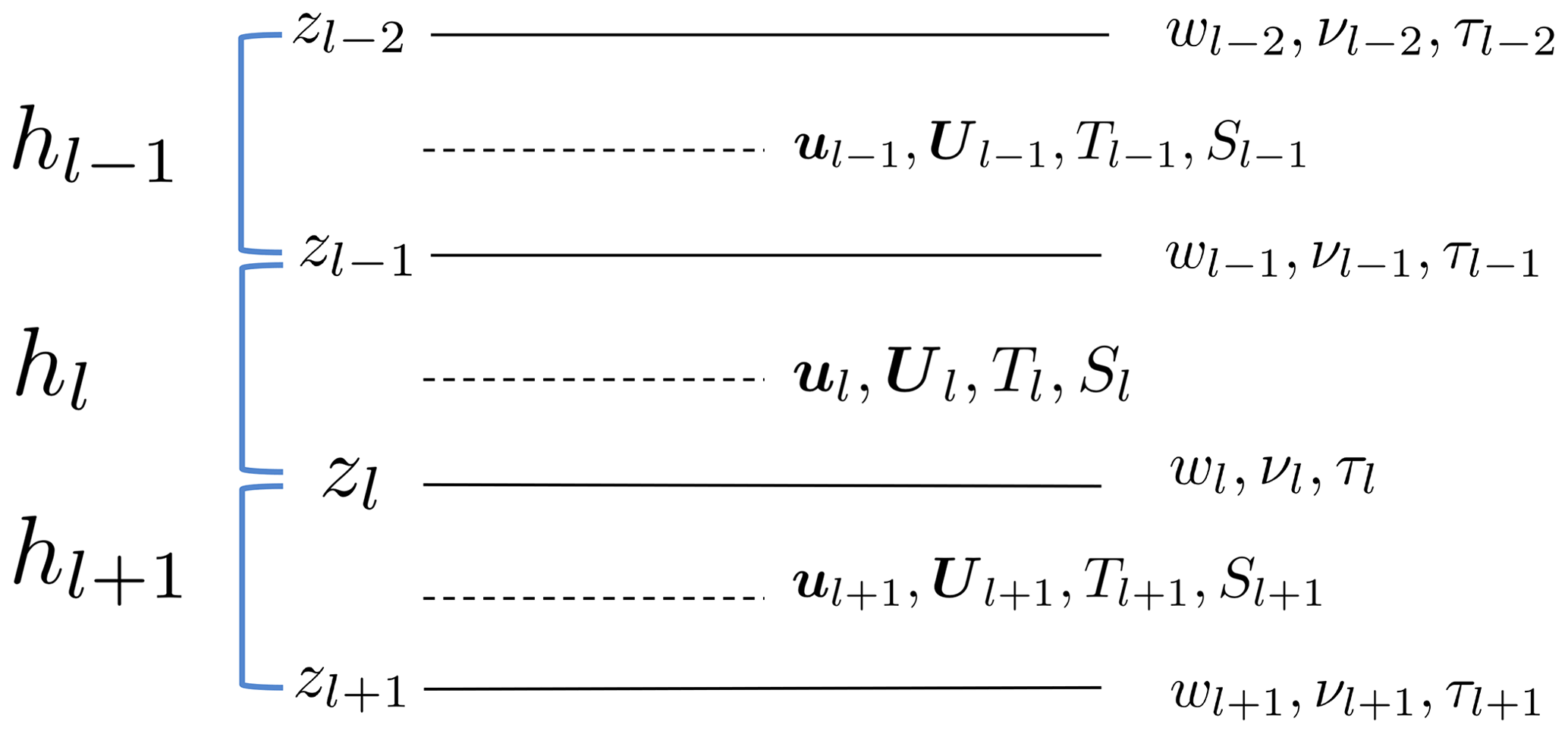
Figure 1 shows how the model variables are staggered over the computational grid. Horizontal momentum (U) is located in the element centers, while all the others are located on the vertexes (vertical velocity w and scalars). Each vertex has a corresponding finite volume (dashed lines in Fig. 1). The staggering of hydrodynamic variables is essential to have a mass-conserving model (Jofre et al., 2014; Felten and Lund, 2006).

Variables are also staggered in the vertical grid, as shown in Fig. 1.

The turbulent and molecular stresses and the vertical velocity are computed at the bottom interface of each layer (black dots in Fig. 1), the free surface is at the top of the upper layer thus determining the variable volume of the top cells, and all the other variables are defined at the layer center (red dots in Fig. 1).

Scalar variables (red) are staggered with respect to vertical velocity (black), referenced in the middle and at layer interfaces, respectively. The sea surface elevation is a 2D field defined only in the w points at surface.

The grid cells on the top layer can change their volume as a result of the oscillation of the free surface. The number of active cells along the vertical direction depends on the sea depth.

The spatial discretization of the governing equations in the finite-element method (FEM) framework is based on the assumption that the approximate solution is a linear combination of shape functions defined in the 2D space. In this section we provide suggestions for the practical use of the FEM method in the relevant terms of the SHYFEM equations.

Table 2 Notation for connectivity and gradient of shape functions.

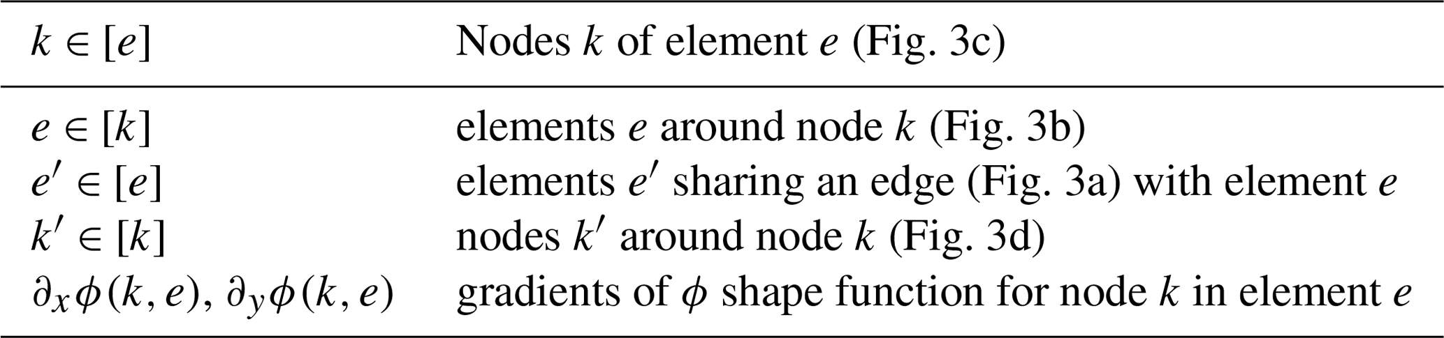
Table 2 reports the possible connectivities that arise from the physics of the SHYFEM equations. Table 2 also shows the definition for the partial derivatives of the linear shape functions to calculate horizontal gradients of scalar quantities and divergence of vector fields. Appendix A gives more insights into the shape functions and the calculation of their gradients.

Considering a scalar field, such as the surface elevation η in Eq. (1), its gradient is a linear combination of the gradient of shape functions.

$$\begin{array}{}\text{(12)}& \begin{array}{rl}& ({\displaystyle \frac{\partial \mathit{\eta }}{\partial x}},{\displaystyle \frac{\partial \mathit{\eta }}{\partial y}}{)}_e\\ & =\left(\sum _{k\in \left[e\right]}{\partial }_x\mathit{\varphi }\right(k,e\left)\mathit{\eta }\right(k),\sum _{k\in \left[e\right]}{\partial }_y\mathit{\varphi }(k,e\left)\mathit{\eta }\right(k\left)\right)\end{array}\end{array}$$

The resulting gradient is referenced to the element e, and is a combination of values referenced to its nodes. This means that the calculation of the horizontal gradient of a scalar field consists of a node-to-element dependency (see Fig. 3c).

Considering a vector field, such as U, its horizontal divergence is a linear combination of the same gradients as the shape functions, as detailed below:

$$\begin{array}{}\text{(13)}& (\mathrm{\nabla }\mathit{U}{)}_k=\sum _{e\in \left[k\right]}{\partial }_x\mathit{\varphi }(k,e\left)U\right(e)+{\partial }_y\mathit{\varphi }(k,e\left)V\right(e),\end{array}$$

where the divergence of the horizontal velocity field is referenced to the node k and is the sum of the momentum fluxes inside/outside the node control volume from the elements surrounding the node e∈[k]. Calculation of the divergence of vector fields consists of an element-to-node dependency (see Fig. 3b).

The horizontal viscosity stress in x direction (and similarly in y direction) has the form

$$\begin{array}{}\text{(14)}& A_H\left(e\right)\sum _{e^{\prime }\in \left[e\right]}{\displaystyle \frac{U\left(e^{\prime }\right)-U\left(e\right)}{\left(A\right(e^{\prime })+A(e\left)\right)/\mathrm{2}}},\end{array}$$

where the contributions come from the differences between the momentum of the current element U(e) and the momentum of surrounding elements e^′ that share one side with e divided by the sum of areas of both elements $A\left(e\right)+A\left(e^{\prime }\right)$. A_H(e) is the viscosity coefficient calculated according to (Smagorinsky, 1963). The viscosity stress components thus consist in an element-to-element dependency (see Fig. 3a).

Equation (4) can be seen in matrix form for $\mathbf{A}{\mathit{\eta }}^{n+\mathrm{1}}=\mathbf{B}$ with $\mathbf{A}=\mathbf{I}+\mathit{\delta }\mathrm{\nabla }\cdot \left(H\mathrm{\nabla }\right)$ and B containing the right-hand side of Eq. (4) as well as η, a column vector containing the values of η at nodes. The left-hand side of Eq. (4) is discretized as follows:

$$\begin{array}{}\text{(15)}& \begin{array}{rl}{\mathit{\eta }}^{n+\mathrm{1}}\left(k\right)+\mathit{\delta }& \sum _{e\in \left[k\right]}\left({\partial }_x\mathit{\varphi }\right(k,e)H_e\\ & \times \sum _{k^{\prime }\in \left[e\right]}{\partial }_x\mathit{\varphi }(k^{\prime },e){\mathit{\eta }}^{n+\mathrm{1}}\left(k^{\prime }\right)+{\partial }_y\mathit{\varphi }(k,e)H_e\\ & \times \sum _{k^{\prime }\in \left[e\right]}{\partial }_y\mathit{\varphi }(k^{\prime },e){\mathit{\eta }}^{n+\mathrm{1}}\left(k^{\prime }\right)),\end{array}\end{array}$$

creating a dependency between node k and the surrounding nodes $k^{\prime }\in \left[k\right]$.

The terms $\mathrm{1}+\mathit{\delta }\left({\partial }_x\mathit{\varphi }\right(k,e\left)H_e{\partial }_x\mathit{\varphi }\right(k^{\prime },e)$ and ${\partial }_y\mathit{\varphi }(k,e)H_e{\partial }_y\mathit{\varphi }(k^{\prime },e))$ represent diagonal entries if $k^{\prime }==k$ and terms $\mathit{\delta }\left({\partial }_x\mathit{\varphi }\right(k,e\left)H_e{\partial }_x\mathit{\varphi }\right(k^{\prime },e)$ and ${\partial }_y\mathit{\varphi }(k,e)H_e{\partial }_y\mathit{\varphi }(k^{\prime },e))$ represent off-diagonal entries in case $k^{\prime }\ne k$.

The dependency between adjacent nodes of η introduced by the discretization of A is of the kind node to node (see Fig. 3d).

3 Parallel approach

Scientific and engineering numerical simulations involve an ever-growing demand for computing resources due to the increasing model resolution and complexity. Computer architectures satisfy simulation requirements through a variety of computing hardware, often combined together into heterogeneous architectures. There are key benefits from the design (or re-design) of a parallel application (Zhang et al., 2020a; Fuhrer et al., 2014) and the choice of parallel paradigm, taking into account the features of computing facilities (Lawrence et al., 2018). Shared and distributed parallel programming can be mixed to better exploit heterogeneous architectures. MPI+X​​​​​​​ enables the code to be executed on clusters of non-uniform memory access (NUMA) nodes equipped with CPUs, GPUs, accelerators, etc. This mixing should be done by taking into account the main features of the two paradigms. The shared memory approach enables multiple processing units to share data but does not allow the problem to be scaled on more than one computing node, setting an upper bound to the available memory. The distributed memory approach, on the other hand, enables each computing process to access its own memory space, so that bigger problems can be addressed by scaling the memory over multiple nodes. However, communication between parallel processes is needed in order to satisfy data dependencies. Given that configurations will require even more memory and computing power, the strategy used to parallelize the SHYFEM model is based on the distributed memory approach with MPI. The parallelization strategy can be easily combined with the existing shared memory implementation based on OpenMP (Pascolo et al., 2016) or with other approaches not yet implemented (e.g., OpenACC).

3.1 The domain partitioning issue

Identifying data dependencies is key for the design of the parallel algorithm, since inter-process communications need to be introduced to satisfy these dependencies.

In the case of a structured grid, each grid point usually holds information related to the cell discretized in the space, and data dependencies are represented by a stencil containing the relations between each cell and its neighbors. For example, we could have five or nine point stencils that represent the dependencies of the current cell with regards to its four neighbors north, south, east and west, or alternatively cells along diagonals could also be considered for computation.

On the other hand, unstructured grid models can be characterized by dependencies among nodes (the vertexes), elements (triangles), or nodes and elements. These kinds of dependencies need to be taken into account when the partitioning strategy is defined.

Figure 2 Element based partitioning and node-based partitioning.

3.2 Partitioning strategy

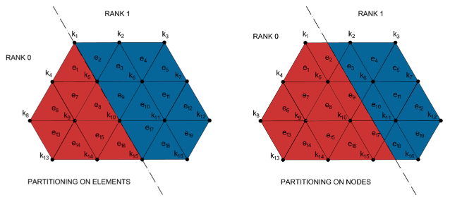
The choice between element-based or node-based partitioning (see Fig. 2) aims to reduce the data exchange among different processes.

The best partitioning strategy cannot be defined absolutely. In fact, it usually depends on the code architecture and its implementation.

Figure 3 Possible data dependencies on a staggered grid.

Analysis of the SHYFEM code shows that an element-based domain decomposition minimizes the number of communications among the parallel processes. Four types of data dependencies (see Fig. 3) were identified within the code: element-to-element (A) – the computation on each element depends on the three adjacent elements; element-to-node (B) – the node receives data from the incident elements (usually six); node-to-element (C) – the element needs data from its three nodes; node-to-node (D) – the computation on each node depends on the adjacent nodes.

The element-based partitioning needs data exchange when there are dependencies A, B and D, while node-based partitioning needs data exchange with dependencies C and D. The data dependency A happens only when momentum is exchanged to compute the viscosity operator; the data dependency D happens in two cases when matrix–vector products are computed for the implicit solution of the free surface equation (FSE) which is solved using the PETSc (Portable, Extensible Toolkit for Scientific Computation) external libraries; finally, the data dependency C is the most common in the code, more frequent than dependency B.

We can thus summarize that, after analyzing the SHYFEM code, element-based partitioning reduces the data dependencies that need to be solved through data exchanges between neighboring processes. Clearly, the computation on nodes shared among different processes is replicated.

3.3 The partitioning algorithm

The second step, after selecting the partitioning strategy, is to define the partitioning algorithm. This represents a way of distributing the workload among the processes for an efficient parallel computation. The standard approach (Hendrickson and Kolda, 2000) is to consider the computational grid as a graph and to apply a graph partitioning strategy in order to distribute the workload. The graph partitioning problem consists in the aggregation of nodes into mutually exclusive groups minimizing the number of cutting edges. The graph partitioning problems fall under the category of NP-hard (non-deterministic polynomial-time hard) problems. Solutions to these problems are generally derived using heuristics and approximation algorithms. There are several parallel tools that provide solutions to the partitioning problem, such as ParMetis (Karypis et al., 1997), the parallel extended version of Metis (Karypis and Kumar, 1999), Jostle (Walshaw and Cross, 2007), PT-Scotch (Chevalier and Pellegrini, 2008) and Zoltan (Hendrickson and Kolda, 2000). The scalability of the Zoltan PHG partitioner (Sivasankaran Rajamanickam, 2012) was a key factor in the choice of the partitioning tool for the parallel version of SHYFEM. The Zoltan library simplifies the development and improves the performance of the parallel applications based on geometrically complex grids. The Zoltan framework includes parallel partitioning algorithms, data migration, parallel graph coloring, distributed data directories, unstructured communication services and memory management packages. It is available as open-source software. An offline static partition module was designed and implemented. It is executed once before beginning the simulation, when the number of parallel processes has been decided. The partitioning phase aims to minimize the inter-process edge cuts and the differences among the workloads assigned to the various processes. The weights used in the graph partitioning for each element are proportional to the number of vertical levels of the element itself.

4 Parallel code implementation

The SHYFEM code has a modular structure. It enables users to customize the execution by changing the parameters defined within a configuration file (i.e., namelist), to set up the simulation, and to activate the modules that solve hydrodynamics, thermodynamics and turbulence.

This section details the changes made to the original code, introducing the additional data structures needed to handle the domain partitioning, the MPI point-to-point and collective communications, the solution of the FSE using the external PETSc library (Balay et al., 1997, 2020, 2021), and the I/O management.

4.1 Local–global mapping

The domain decomposition over several MPI processes entails mapping the information of local entities to global entities. The entities to be mapped are the elements and nodes. As a consequence of the partitioning procedure, each process holds two mapping tables, one for the elements and one for the nodes. The mapping table of the elements stores the correspondence between the global identifier of the element (which is globally unique) with a local identifier of the same element (which is locally unique). The same also happens with the mapping table associated with the nodes. Mapping information is stored within two local data structures, containing the global identification number (GID) of elements and nodes. The order of GID elements in local structures is natural; namely they are set in ascending order of GIDs. The local–global mapping is represented by the position in the local structure of the GIDs, called local identification number (LID).

The GIDs of the nodes are stored in a different order. The GIDs of the nodes that belong to the boundary of the local domain are stored at the end of the mapping table. This provides some computational benefits: it is easy to identify all of the nodes on the border; in most cases it is better to first execute the computation over all of the nodes in the inner domain and after the computation over the nodes at the boundary; during the data exchange it is easy to identify which nodes need to be sent and which ones need to be updated with the data from the neighboring processes.

4.2 Data exchange

Data exchanges are executed when element-to-node and element-to-element dependencies happen and MPI point-to-point communications are used. In the first case, each process receives information based on the elements that share the target node from the processes the elements belong to. It keeps track of the shared nodes in terms of numbers and LIDs. Each process computes the local contribution and sends it to the interested neighboring processes. The information received is stored in a temporary 3D data structure defined for nodes, vertical levels and processes. A reduction operation is performed on the information received.

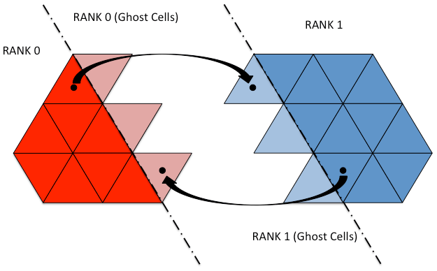
The element-to-element dependency happens only once in the time loop required to compute the viscosity operator. In this case, each process sends its contribution to the neighbors in terms of momentum values. Each process keeps track of the elements to be sent/received in terms of the numbers and LIDs, using two different data structures. In this case, the data structure extends the local domain in order to include an overlap used to store the data received from the neighbors as shown in Fig. 4. Non-blocking point-to-point communications are used to overlap computation and communications.

Figure 4 Communication pattern for the calculation of horizontal viscosity.

Finally, collective communications were introduced to compute properties related to the whole domain, for instance to calculate the minimum or maximum temperature of the basin or to calculate the total water volume. Algorithm 2 reports the pseudo-code of the parallel implementation of the SHYFEM model.

Algorithm 2 SHYFEM-MPI time loop

Require:

𝒩 {Set of neighboring processes}

𝒰, 𝒱 {Set of nodes and edges defined in the current subdomain}

for all p_i∈𝒩 do

SendHalo(𝒰, 𝒱, p_i)

end for

while t<num_timesteps do

for all p_i∈𝒩 do

RecvHalo(𝒰, 𝒱, p_i)

end for

SetExplicitTerms

AdvanceMomentum {Eq. (1)}

GlobalExchange(RHS)

SolveBarotropicEquation {Eq. (4)}

FinaliseMomentum {Eq. (5)}

for all p_i∈𝒩 do

SendHalo(𝒰, 𝒱, p_i)

end for

CalcVerticalVelocity {Eq. (6)}

SolveTracerAdvection {Eq. (7)}

UpdateDensity {Eq. (10)}

end while

4.3 Semi-implicit method for free surface equation

Semi-implicit schemes are common in computational fluid dynamics (CFD) mainly due to the numerical stability of the solution. In the case of ocean numerical modeling, external gravity waves are the fastest process and propagate at a speed of up to 200 m s⁻¹, which puts a strong constraint on the model time step in order to abide by the Courant–Friedrichs–Levy (CFL) condition for the convergence of the solution.

The semi-implicit treatment of barotropic pressure gradient, described in Sect. 2.1, involves the solution of the matrix system

$$\begin{array}{}\text{(16)}& \mathbf{A}{\mathit{\eta }}^{n+\mathrm{1}}=\mathit{B},\end{array}$$

where A is the matrix of coefficients that arise from the FEM discretization of derivatives of the left-hand side of Eq. (4), η is a column vector containing the solution of η with the same size of B, with size nkn×nkn, and B is the vector of the right-hand side of Eq. (4). The matrix A is non-singular with an irregular sparse structure. We used PETSc to solve this equation efficiently.

Iterative methods are the most convenient methods to solve a large sparse system with A not having particular structure properties since the direct inversion of A would be much too expensive. These methods search for an approximate solution for Eq. (16) and include Jacobi, Gauss–Seidel, successive over-relaxation (SOR) and Krylov subspace methods (KSP). KSP is regarded as one of the most important classes of numerical methods.

Algorithms based on KSP search for an approximate solution in the space generated by the matrix A,

$$\begin{array}{}\text{(17)}& {\mathit{\varkappa }}_m(\mathbf{A},{\mathit{v}}_{\mathrm{0}})=\mathrm{span}\mathit{\{}{\mathit{v}}_{\mathrm{0}},\mathbf{A}{\mathit{v}}_{\mathrm{0}},{\mathbf{A}}^{\mathrm{2}}{\mathit{v}}_{\mathrm{0}},\mathrm{\dots },{\mathbf{A}}^{m-\mathrm{1}}{\mathit{v}}_{\mathrm{0}}\mathit{\}},\end{array}$$

called the mth-order Krylov subspace, where v₀ is an arbitrary vector (generally the right-hand side of the system) with the property that the approximate solution x_m belongs to this subspace. In the iterative methods based on KSP, the subspace ϰ_m(A,v₀) is enlarged a finite number of times (m), where x_m  represent an acceptable approximate solution, giving a residual ${\mathit{r}}_m=\mathit{B}-\mathbf{A}{\mathit{x}}_m$ that has a smaller norm than a certain tolerance.

In a parallel application, each of the m iterations is marked out by a computational cost and a communication cost to calculate the matrix–vector products in ϰ_m(A,v₀), since both the matrix and the vector are distributed across the processes. A further cost is the convergence test, which is generally based on the Euclidean norm of the residual.

$$\begin{array}{}\text{(18)}& \begin{array}{rl}& \text{Convergence test}=\\ & \left\{\begin{array}{ll}\left|{\mathit{r}}_m\right|<a_{\text{tol}},& \text{using\hspace{0.17em} absolute\hspace{0.17em} tolerance }\\ \left|{\mathit{r}}_m\right|/\left|B\right|\le r_{\text{tol}},& \text{using\hspace{0.17em} relative\hspace{0.17em} tolerance}\\ \left|{\mathit{r}}_m\right|>d_{\text{tol}},& \text{residual\hspace{0.17em} is\hspace{0.17em} larger\hspace{0.17em} than}\\ & \text{divergence\hspace{0.17em} tolerance}\\ n_{\text{iters}}\ge {max}_{\text{iters}},& \text{the\hspace{0.17em} number\hspace{0.17em} of\hspace{0.17em} iterations}\\ & \text{exceeds\hspace{0.17em} the\hspace{0.17em} maximum}\\ & \text{number\hspace{0.17em} of\hspace{0.17em} iterations}\end{array}\right.\end{array}\end{array}$$

The last two criteria are met when the method diverges.

The calculation of the norm involves global communication to enable all the processes to have the same norm value. Hence both point-to-point and global communication burden each iteration, leading to a loss of efficiency for the parallel application if the number of necessary iterations is high. The number of iterations depends on the physical problem and on its size. An estimate of the problem complexity is given by the condition number C(A), which, for real symmetric matrices, is the ratio $max\left(\mathit{\lambda }\right)/min\left(\mathit{\lambda }\right)$ between the maximum and minimum of the eigenvalues λ of A. In general, the higher C, the more iterations are necessary. The number of iterations also depends on the tolerance desired.

In the case of complex systems it is convenient to modify the original linear system defined in Eq. (16) to get a better Krylov subspace using a further matrix M, called the preconditioner, to search for an approximate solution in the modified system:

$$\begin{array}{}\text{(19)}& {\mathbf{M}}^{-\mathrm{1}}\mathbf{A}x={\mathbf{M}}^{-\mathrm{1}}\mathit{B},\end{array}$$

where ${\mathbf{M}}^{-\mathrm{1}}\approx {\mathbf{A}}^{-\mathrm{1}}$ and is computed easily.

We used PETSc rather than implementing an internal parallel solver. In fact, PETSc was developed specifically to solve problems that arise from partial differential equations on parallel architectures and provides a wide variety of solver/preconditioners that can be switched through a namelist. In addition, the interface to PETSc is independent of the version, and its implementation is highly portable on heterogeneous architectures.

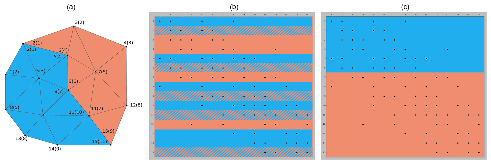
Figure 5 Example of domain decomposition between two MPI processes for SHYFEM-MPI and the PETSc library. Numbers represent the global (local) ID. Panels (c) and (b) represent the matrix A within PETSc and SHYFEM-MPI, respectively.

Figure 6 Data management related to the forcing files and restart files.

The PETSc interface creates counterparts of A and B as objects of the package. A is created as a sparse matrix in coordinate format (row, column, value) using the global ID (see Fig. 5) of the nodes. This is in order to have the same non-zero pattern as the sequential case, regardless of the way the domain is decomposed. The same global ID is used to build the right-hand side B.

To solve the free surface in SHYFEM-MPI, we used the flexible biconjugate gradient stabilized method (FBCGSR) with incomplete lower–upper (iLU) factorization as a preconditioner. We set absolute and relative tolerance to 10⁻¹² and 10⁻¹⁵, respectively. Divergence tolerance and maximum iterations are set to default values (both 10⁴).

The PETSc library uses a parallel algorithm to solve the linear equations. The decomposition used inside PETSc is different from the domain decomposition used in SHYFEM-MPI (see Fig. 5). PETSc divides the matrix A in ascending order with the global ID. The SHYFEM-MPI partitioning is based on criteria that take into account the geometry of the mesh and is, at any rate, different from PETSc. For this reason, after the approximate solution for ηⁿ⁺¹ has been found by PETSc, the solution vector is gathered by the master process and is redistributed across the MPI processes. The time needed to exchange data between the PETSc representation and the model has been estimated to range from 1 % with a low number of cores used up to 10 % of the overall execution time.

Figure 7 Domain of the SANIFS configuration. The model mesh is superimposed over bathymetry.

4.4 I/O management

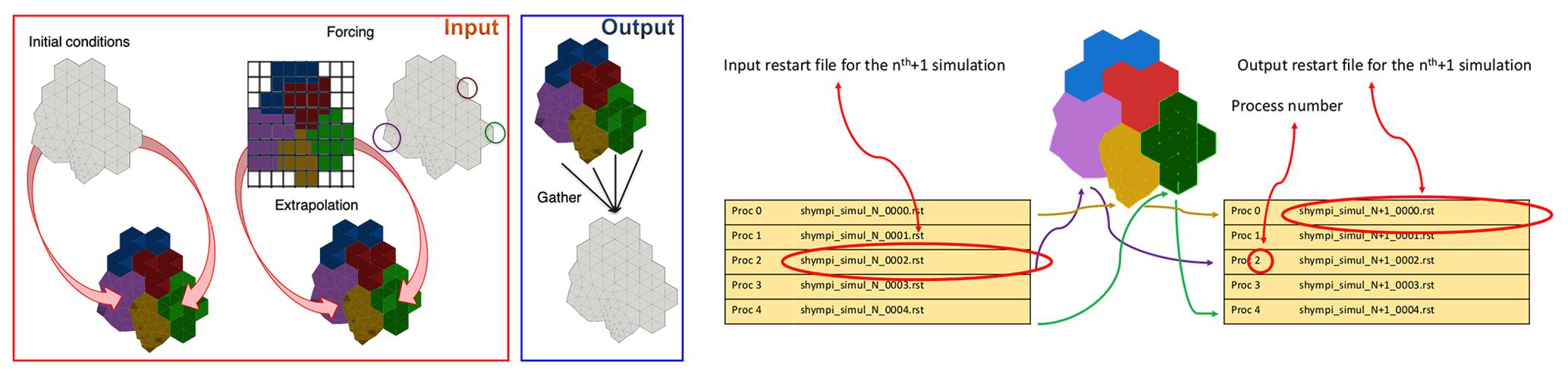
I/O management usually represents a bottleneck in a parallel application. To avoid this, input and output files should be concurrently accessed by the parallel processes, and each process should load its own data. However, loading the whole file for each process would affect memory scalability. In fact, the allocated memory should be independent of the number of parallel processes in order to ensure the memory scalability of the code. The two issues can be addressed by distributing the I/O operations among the parallel processes. During the initialization phase, SHYFEM needs to read two files: the basin geometry and the namelist. All the MPI processes perform the same operation and store common information. This phase is not scalable because each process browses the files. However, this operation is only performed once and has a limited impact on the total execution time. As a second step, initial conditions and forcing (both lateral and surface) are accessed by all the parallel processes, but each one reads its own portion of data, as shown in Fig. 6. Surface atmospheric forcing is defined on a structured grid, so after reading the forcing file, each process interpolates the data on the unstructured grid used by the model. The output can be written using external parallel libraries capable of handling parallel I/O. In this regard, we are evaluating the adoption of efficient external libraries to enhance the I/O for the next version of the model code. Among the suitable I/O libraries we mention here XIOS, PIO, SCORPIO or ADIOS. A check-pointing mechanism was implemented in the parallel version of the model. This is usual when the simulation is divided into dependent chunks in order to maintain the status. Both phases (reading/writing) are performed in a distributed way among the processes to reduce the impact on the parallel speedup of the model, as shown in Fig. 6. Each process generates its own restart file related to its sub-domain and reads its own restart file.

5 Results

We ran our experiments to assess the correctness of MPI implementation on the Southern Adriatic Northern Ionian coastal Forecasting System (SANIFS) configuration, which has a horizontal resolution of 500 m near the coast of up to 3–4 km in open waters. The total number of grid elements is 176 331. Vertical resolution is 2 m near the surface stepwise increasing towards the sea bottom, dividing the water column into 80 layers. For details of the model grid and the system settings, see Federico et al. (2017).

Runs are initialized with the motionless velocity field and with temperature and salinity fields from CMEMS NRT products (Clementi et al., 2019). The simulations are forced hourly at lateral boundaries with water level fields, total velocities and active tracers from the same products.

The sea level is imposed with a Dirichlet condition, while relaxation is applied to the parent model total velocities with a relaxation time of 1 h. For scalars, the inner values are advected outside the domain when the flow is outwards, while a Dirichlet condition is applied for inflows.

The boundary conditions for the upper surface follow the MFS bulk formulation (Pettenuzzo et al., 2010), which requires wind, cloud cover, air and dew point temperature, available in ECMWF analysis, with a temporal/spatial resolution of 6 h/0.125^∘​​​​​​​, respectively. From the same analysis, we force the surface with precipitation data.

We select an upwind scheme for both horizontal and vertical tracer advections. The formulation of bottom stress is quadratic. The time stepping for the hydrodynamics is semi-implicit with $\mathit{\gamma }=\mathit{\beta }=\mathrm{0.6}$. Horizontal viscosity/diffusivity follows the formulation of Smagorinsky (1963). Turbulent viscosity/diffusivity is set to a constant value equal to 10⁻³ m² s⁻¹.

The cold start implies strong baroclinic gradients. To prevent instabilities, we select a relatively small time step, set to Δt = 15 s.

5.1 SHYFEM-MPI model validation

The round-off error, given by the representation of floating point numbers, affects all the scientific applications based on numerical solutions including general circulation models (GCMs). The computational error, such as the round-off error, is present also in the sequential version of all numerical models. The round-off error is the main reason why when the same sequential code is executed on different computational architectures or it is executed with different compiler options or with different compilers, the outputs are not bit-to-bit identical. Moreover, only changing the order of the evaluation of the elements in the domain using the sequential version of SHYFEM we obtain outputs which are not bit-to-bit identical. The parallel implementation through MPI inherently leads to a different order in the evaluation of elements and hence a different order in the floating point operations. Although we can force the MPI version to execute the floating point operations in the same order of the sequential version and then the parallel model results are the same as those of the serial model, we cannot guarantee that the results of the serial model have no uncertainty because the serial model also contains the round-off error. Cousins and Xue (2001) developed the parallel version of the Princeton Ocean Model (POM) and found that there is a significant difference between the serial and parallel version of the POM, concluding that the error from the data communication process via MPI is the main reason for the difference. Wang et al. (2007) studied the results of the atmospheric model SAMIL simulated with different CPUs and pointed out that the difference is chiefly caused by the round-off error. Song et al. (2012) assessed the round-off error impact, due to MPI, on the parallel implementation of the Community Climate System Model (CCSM3). Guarino et al. (2020) presented the evaluation of the reproducibility of the HadGEM3-GC3.1 model on different HPC platforms. Geyer et al. (2021) assessed the limit of reproducibility of the COSMO-CLM5.0 model comparing the same code executed on different computational architectures. Their analysis showed that the simulation results are dependent on the computational environments and the magnitude of uncertainty due to the parallel computational error could be in the same order as that of natural variations in the climate system.

The parallel implementation of the SHYFEM model was validated to assess the reproducibility of the results when varying the size of the domain decomposition and the number of parallel cores used for a simulation. Our baseline was the results from a sequential run, and we compared the results with those obtained with parallel simulations on 36, 72, 108 and 216 cores. The parallel architecture used for the tests is named Zeus and is available at the CMCC Supercomputing Center. Zeus is a parallel machine equipped with 348 parallel nodes interconnected with an Infiniband EDR (100 Gbps) switch. Each node has two Intel Xeon Gold 6154 (18 cores) CPUs and 96 GB of main memory.

The results were compared with a 1 d simulation, saving the outputs every hour (the model executes 5760 time steps) and referring to the data from the native grid. Only the most significative fields were taken into account for comparison: temperature, salinity, sea surface high and zonal velocity. In order to evaluate the differences between the parallel execution with respect to the results obtained with a sequential run, we used the root mean square error as a metric:

$$\text{RMSE}(X,Y)=\sqrt{{\displaystyle \frac{{\sum }_i\left((X_i-Y_i{)}^{\mathrm{2}}\right)}{N}}}.$$

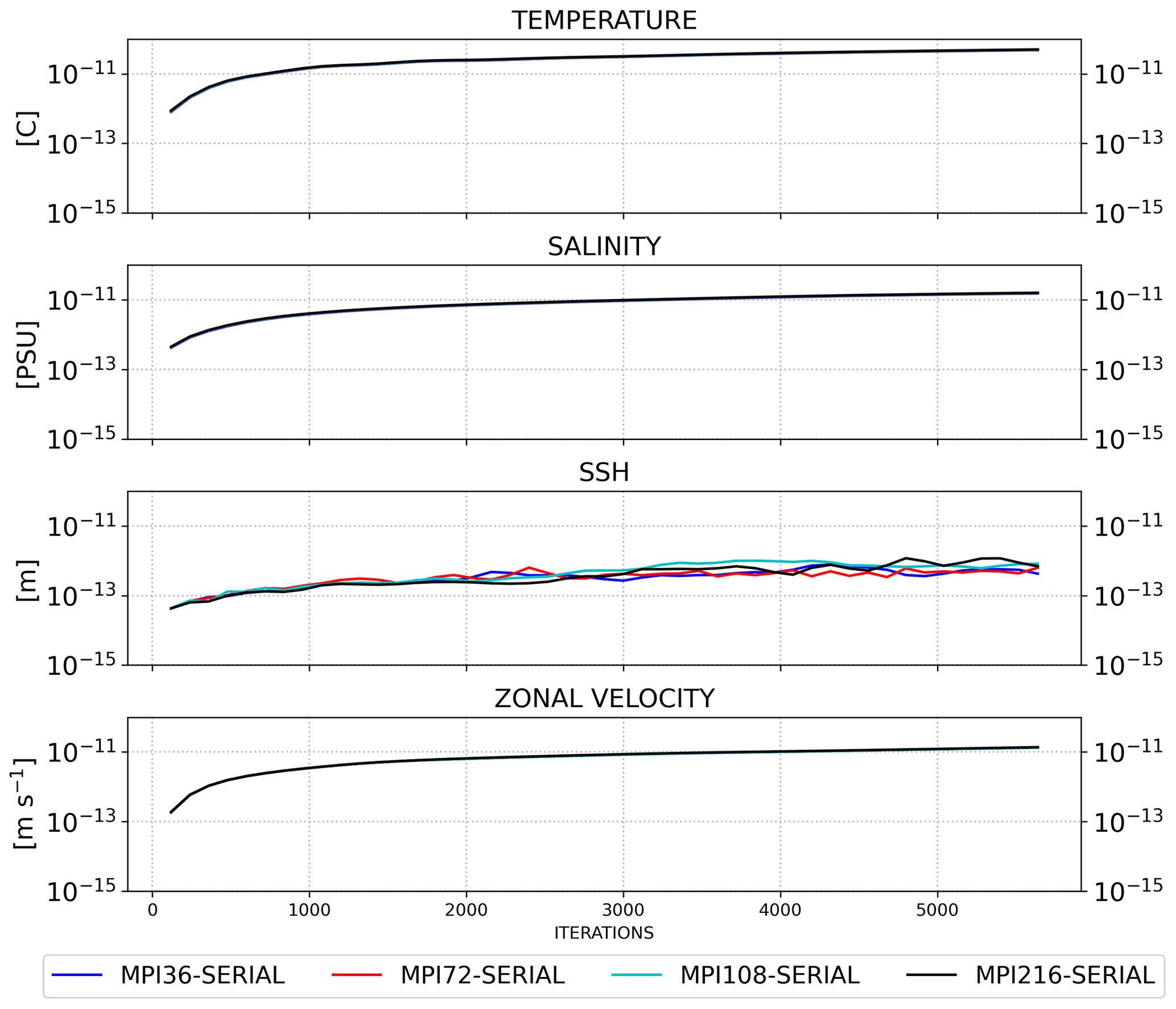
Figure 8 RMSE time series of SHYFEM-MPI outputs compared with the sequential run for all the prognostic fields and with different numbers of cores: 36, 72, 108 and 216.

As a result, we computed the RMSE for each domain decomposition, for each aforementioned field and for each time step saved in the output files (hourly), as shown in Fig. 8. The RMSE time series were calculated using NCOoperators applied to the output on the native SHYFEM-MPI grid considering all the active cells in the domain.

The time series of all the MPI decompositions overlap, which means that the program can reproduce the sequential result close to machine precision. The time series of the sea surface height (SSH) are noisy, but the RMSE remains steady and of the order of 10⁻¹³. The SHYFEM-MPI model is not bit-to-bit reproducible for two main reasons. The field values computed on the grid nodes belonging to the border between two domains are computed first by the two processes independently, taking into account only the node neighbors in the local domain, thus giving a partial value. The partial values are then exchanged between the two processes, and the final value is computed with a sum of the partial values. The order of the floating point operations, executed on the grid nodes at the border, thus changes when the domain decomposition changes, creating a numerical difference between two simulations that use a different number of cores. In fact, the floating point operations lose their associative property due to the approximate representation of the numbers (Goldberg, 1991). The second source of non bit-to-bit reproducibility is due to the optimized implementation of the PETSc numerical library, which makes use of non-blocking MPI communications. This, in turn, creates a non-deterministic order in the execution of the floating point operations, which generates a numerical difference even between two different executions of the same configuration with the same domain decomposition and the same number of cores.

To further assess the impact of the round-off error induced by the use of PETSc solver, we ran the same configuration five times with the same number of cores. Again we used the RMSE as a metric to quantify the differences between four simulations with respect to the first one, which was taken as reference. Figure 9 shows the RMSE time series of the simulations executed with 72 cores.

Figure 9 RMSE evaluated for code reproducibility with 72 MPI processes.

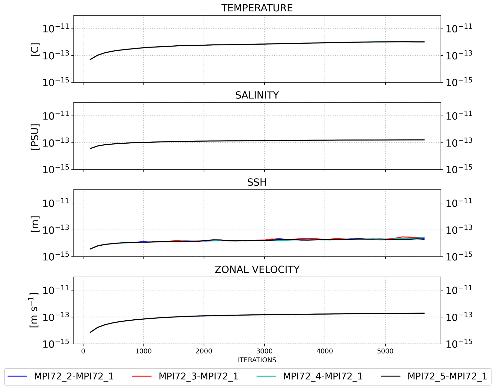
Although the SHYFEM-MPI implementation is not bit-to-bit reproducible, the RMSE time series show that for each of the model variables, the deviations of the runs from the reference run remain close to the machine precision, with no effect on the reproducibility of the solution of the physical problem. We implemented a perfect reproducible version of the model by including a halo over the elements shared between the neighboring processes. This version can be obtained using the DEBUGON compiler key while compiling the code. This ensures that the order of the floating point operations is kept the same and forces the PETSc solver for sequential use. However, this version is only for debugging and is beyond the scope of this work. Moreover, we tested the restartability of the code comparing the results obtained from a run, a.k.a. the long run, simulating 1 d, but writing the restart files after 12 h and running a short run, simulating a half-day, starting from the restart files produced by the long run. The outputs of both simulations are bit-to-bit identical. For this experiment we used the model compiled in reproducible mode.

Figure 10 Execution time in a log–log plot of different solvers available in the PETSc library.

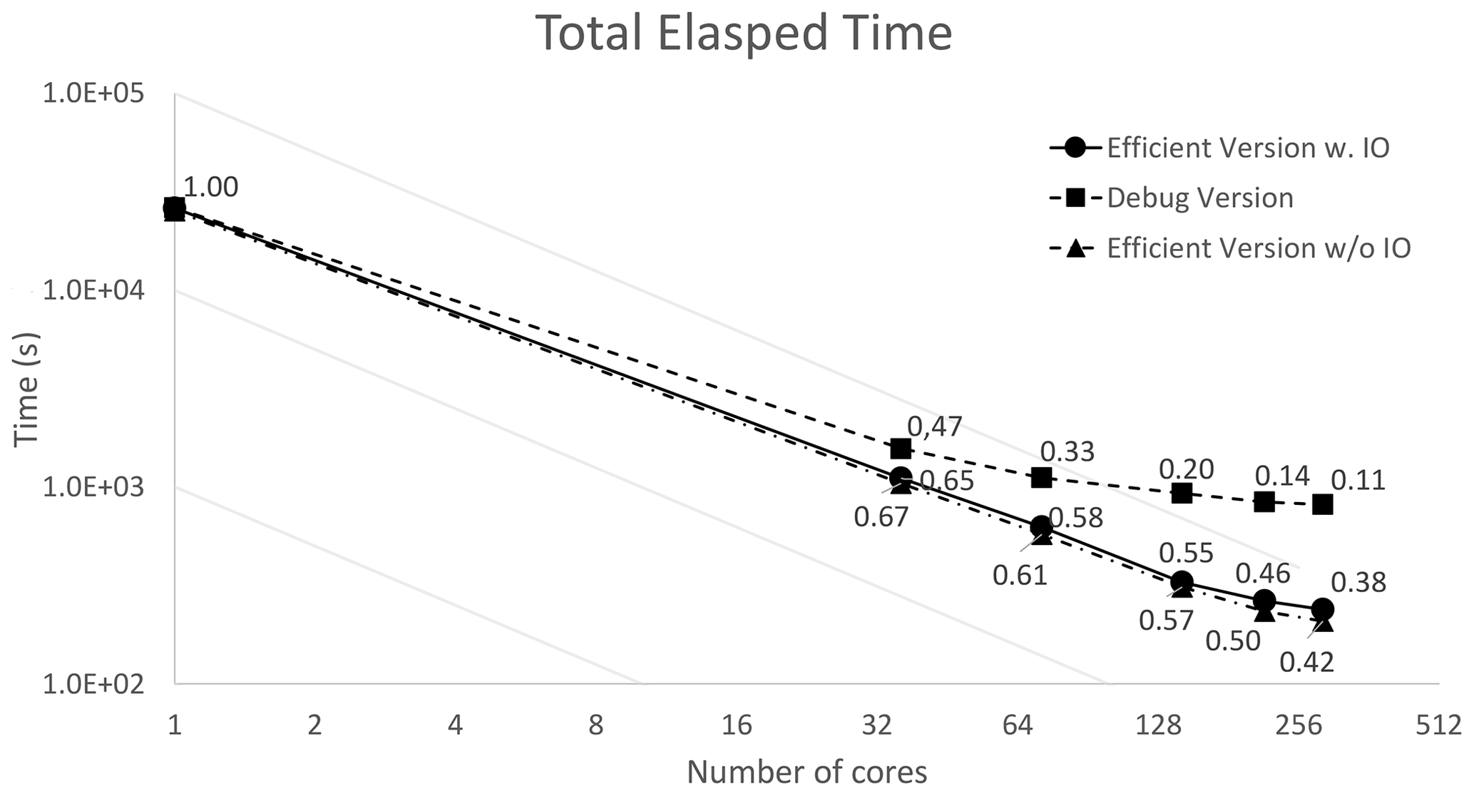
Figure 11 SANIFS execution time in a log–log plot of three settings of the code: efficient MPI version of the code including I/O; efficient MPI version of the code without I/O; debug version of the code which reproduces bit-to-bit identical output of the sequential version.

5.2 SHYFEM-MPI performance assessment

The parallel scalability of the SHYFEM-MPI model was evaluated on Zeus parallel architecture. The SANIFS configuration was simulated for 7 d and the number of cores varied up to 288, which corresponds to eight nodes of the Zeus supercomputer (each node is equipped with 36 cores).

The SHYFEM-MPI implementation relies on the PETSc numerical library, which provides a wide range of numerical solvers. As a preliminary evaluation, we compared the computational performance of the following solvers: the generalized minimal residual (GMRES) method, the improved biconjugate gradient stabilized method (IBCGS), the flexible biconjugate gradient stabilized (FBCGSR) method and the biconjugate gradient stabilized method (BCGS). The pipelined solvers available in the PETSc library aim at hiding network latencies and synchronizations which can become computational bottlenecks in Krylov methods. Among the available pipelined solvers we tested pipelined variant of the biconjugate gradient stabilized method (PIPEBGCS) and the pipelined variant of the generalized minimal residual method (PIPEBCGS). The former method diverges after a few iterations; it was necessary to increase the tolerances by 4 orders of magnitude in order to use it, and it did not lead to improvements. The latter instead had a worse scalability than the BCGS method used initially. Finally, we experimented with the use of the free-matrix approach also available in the PETSc library, which does not require explicit storage of the matrix, for the numerical solution of partial differential equations. The results reported in Fig. 10 show that the FBCGSR solver performs better.

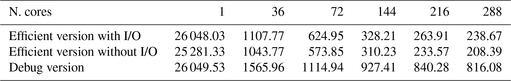
Table 3 Execution time when scaling the number of computational cores of the efficient MPI version of the model with and without I/O and of the debug version of the code. Time is expressed in seconds.

To assess the decoupled effect of the I/O and computational performance of the model, we ran the model with the configuration that does not write the output, so that the MPI implementation can be clearly assessed. Since I/O can be affected by its way of implementation in the model and the architecture of the underlying system (number of I/O nodes, their interconnection, number of MDS and OSS servers, RAID configuration, and the parallel file system used) it would be hard to assess the effect of the I/O in the benchmark results and could add extra uncertainty to the performance measurements and results.

We hence evaluated the model with the SANIFS configuration including the effect of I/O to provide an insight into the model performance when a realistic configuration is used. Finally we measured the speedup of the debug version of the model, which provides the bit-to-bit identical outputs of the sequential version. Figure 11 shows a comparison of the total execution time in a log–log plot where the parallel scalability can also be evaluated. In fact, the behavior of an ideal scalability results in a straight line in the log–log plot. The labels associated with each point in the plot represent the parallel efficiency. The efficiency drops below 40 % with 288 cores, which can thus be regarded as the scalability bound of the model for the SANIFS configuration.

In Table 3 we report the detailed execution times of the computational performance benchmarks.

Figure 12 SANIFS detailed execution time for different processing phases.

Deeper insights into the performances are provided in Fig. 12, which reports the execution time for different processing steps of the model. The execution time was partitioned between the routines to evaluate the momentum equation, advection/diffusion equation, sea level equation (which involves the PETSc solver), the MPI communication time and the I/O. The results demonstrate a very good scalability for the momentum and tracer processing steps, while the sea level computation which involves the numerical solver does not scale as well as the other parts of the model. The communication time also includes the idle time required for waiting for the slowest process to reach the communication call. The idle time can be reduced by enhancing the work load balance among the processes. Although the time spent for I/O is completely unscalable, it is not a limiting factor in this experiment since it is 2 orders of magnitude smaller than the other processing steps.

Figure 13 SANIFS processing ratio among the computing phases.

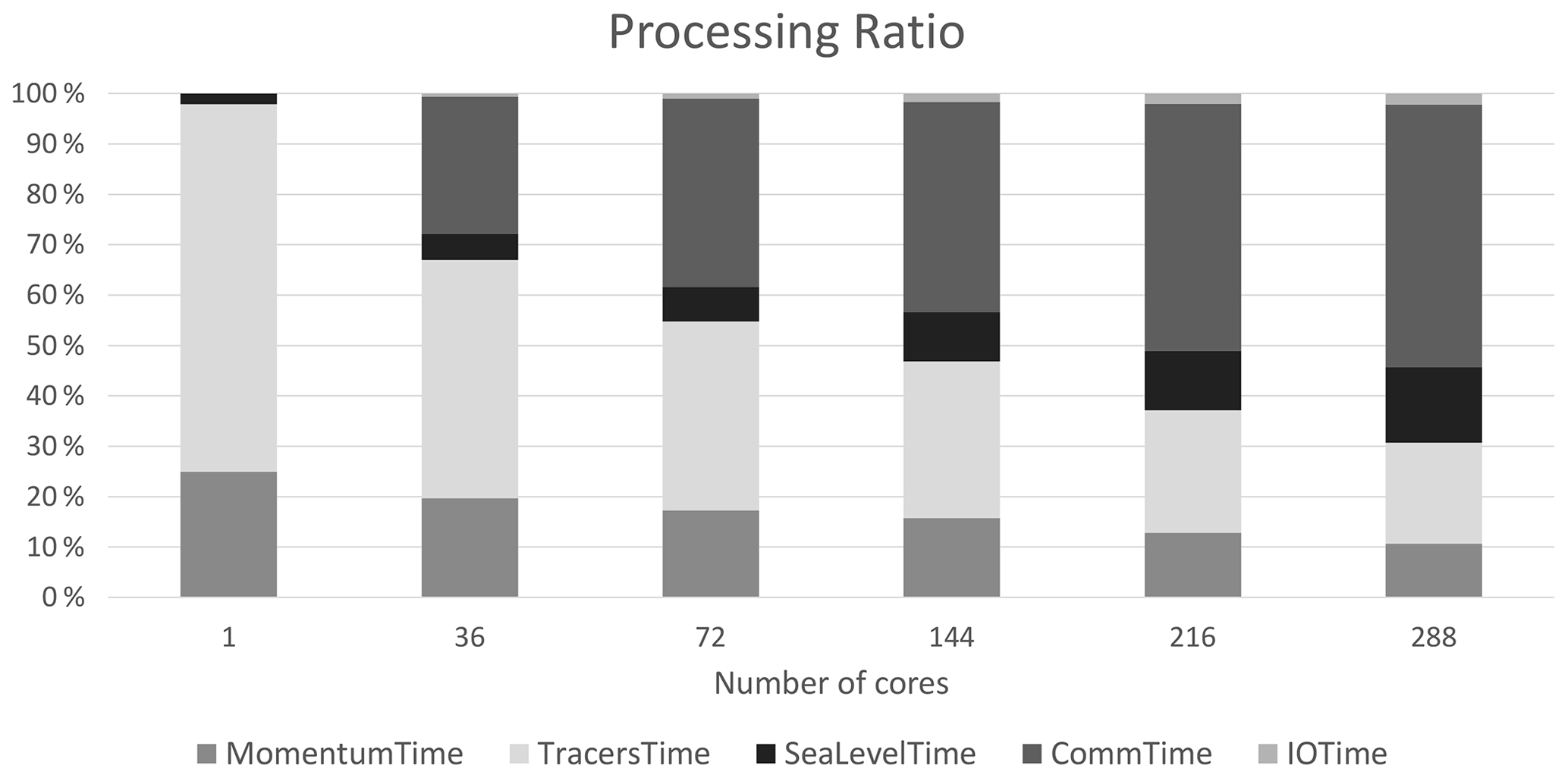
Figure 13 shows the ratio in the execution time of the model's processing steps. The evaluation of the momentum equation and the advection/diffusion equation take most of the execution time in the sequential run. Increasing the MPI processes, the ratios among these components change, and the communication cost becomes an increasing burden on the total execution time.

Finally, we measured the memory footprint of the model varying the number of processors. Figure 14 reports the memory allocation per node when the model is executed on one node up to eight nodes. The results show a good memory scalability. The labels on each point represent the allocated memory per node expressed in megabytes.

Figure 14 SANIFS memory usage with different number of computing nodes. The labels on the points refer to the memory per node expressed in MB.

To conclude, the free surface equation part of the code needs to be better investigated for a more efficient parallelization. Among the investigations we started to evaluate the use of high-level numerical libraries such as Trilinos and Hypre and the exploitation of the DMPlex module available in the PETSc package to efficiently handle the unstructured grids. The execution time reported for the free surface solver includes the assembly of the linear system, the communication time of the internal routines of PETSc for each of the solver iterations and the communication needed to redistribute the solution onto the model grid. The effects of a non-optimal model mesh partitioning on the solver efficiency have not yet been assessed. Moreover, a more efficient partition algorithm should be adopted to reduce the idle time and to improve the load balancing.

6 Conclusions

The hydrodynamical core of SHYFEM is parallelized with a distributed memory strategy, allowing for both calculation and memory scalability. The implementation of the parallel version includes external libraries for domain partitioning and the solution of the free surface equation. The parallel code was validated using a realistic configuration as a benchmark. The optimized version of the parallel model does not reproduce the output of the sequential code bit to bit but reproduces the physics of the problem without significant differences with respect to the sequential run. The source of these differences was considered for different orders of operations in each of the domain decompositions. Forcing the code to exactly reproduce the order of the operation in the sequential code was found to lead to a dramatic loss of efficiency and was therefore not considered in this work.

Our assessment reveals that the limit of scalability in the parallel code is reached at 288 MPI cores, when the parallel efficiency drops below 40 %. The analysis of the parallel performance indicates that with a high level of MPI processes used, the burden of communication and the cost of solving the free surface equation take up a huge proportion of the single model time step. The workload balance needs to be improved, with a more suitable solution for domain partitioning. The parallel code, however, enables one of the main tasks of this work to be accomplished, namely to obtain the results of the simulation in a time that is reasonable and significantly faster than the sequential case. The benchmark has demonstrated that the execution time is reduced from nearly 8 h for the sequential run to less than 4 min with 288 MPI cores.

Appendix A: Linear shape functions

A continuous function f(x,y) in the 2D space can be represented in a discrete mesh as a linear combination of base functions ϕ_k:

$$\begin{array}{}\text{(A1)}& f(x,y)\approx \sum _k{\mathit{\varphi }}_k(x,y)f_k,\end{array}$$

where f_k denote the coefficients of the functions that approximate f. In the context of SHYFEM, ϕ functions are node-referenced linear functions that overlap only in elements in common between adjacent nodes. In particular, the shape function of a node k is 1 on k and 0 on the others (see Fig. A1).

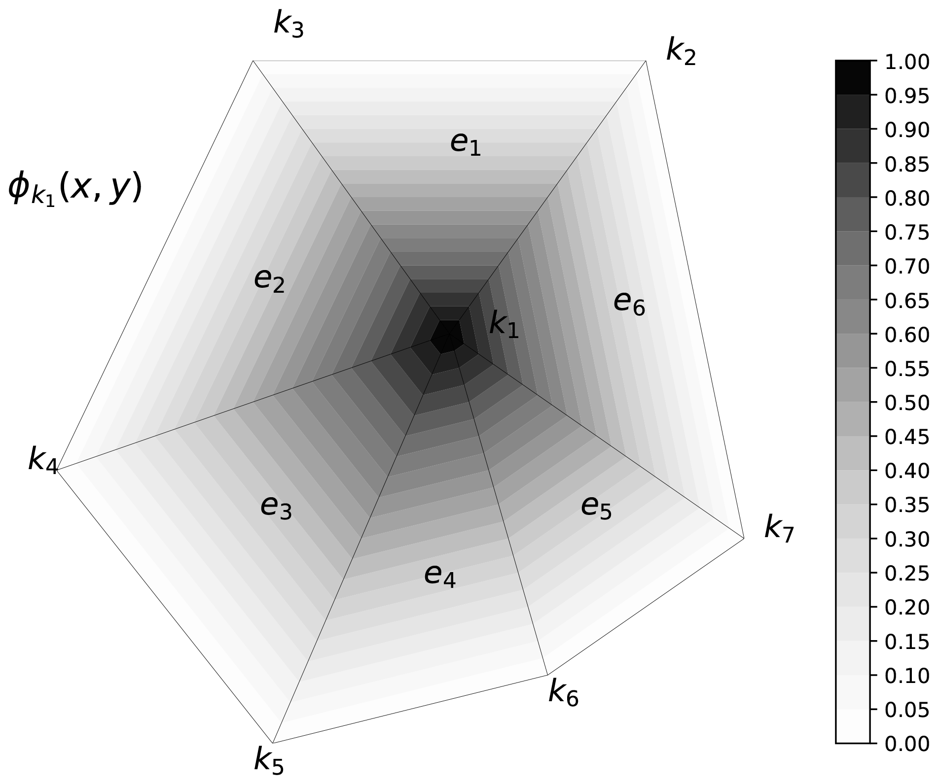
Figure A1 Shape function of node k₁. The function is 1 in k₁ and 0 in all the other nodes. ${\mathit{\varphi }}_{k_{\mathrm{1}}}(x,y)$ overlaps only with the shape functions associated with neighboring nodes.

Considering an element e with its three nodes (k₁, k₂, k₃) of coordinates (x₁,y₁), (x₂,y₂), (x₃,y₃) with the corresponding values (f₁, f₂, f₃) of f we are interested in the gradient of f within the element e. We consider the shape functions that overlap in this element as ${\mathit{\varphi }}_{k_{\mathrm{1}},e}$, ${\mathit{\varphi }}_{k_{\mathrm{2}},e}$, ${\mathit{\varphi }}_{k_{\mathrm{3}},e}$ (see Fig. A2) with the following constraints:

$$\begin{array}{}\text{(A2)}& {\displaystyle }f(x,y)& {\displaystyle }=f_{\mathrm{1}}{\mathit{\varphi }}_{k_{\mathrm{1}},e}+f_{\mathrm{2}}{\mathit{\varphi }}_{k_{\mathrm{2}},e}+f_{\mathrm{3}}{\mathit{\varphi }}_{k_{\mathrm{3}},e},\text{(A3)}& {\displaystyle \frac{\partial f}{\partial x}}& {\displaystyle }=f_{\mathrm{1}}{\displaystyle \frac{\partial {\mathit{\varphi }}_{k_{\mathrm{1}},e}}{\partial x}}+f_{\mathrm{2}}{\displaystyle \frac{\partial {\mathit{\varphi }}_{k\mathrm{2},e}}{\partial x}}+f_{\mathrm{3}}{\displaystyle \frac{\partial {\mathit{\varphi }}_{k\mathrm{3},e}}{\partial x}},\text{(A4)}& {\displaystyle \frac{\partial f}{\partial y}}& {\displaystyle }=f_{\mathrm{1}}{\displaystyle \frac{\partial {\mathit{\varphi }}_{k_{\mathrm{1}},e}}{\partial y}}+f_{\mathrm{2}}{\displaystyle \frac{\partial {\mathit{\varphi }}_{k_{\mathrm{2}},e}}{\partial y}}+f_{\mathrm{3}}{\displaystyle \frac{\partial {\mathit{\varphi }}_{k_{\mathrm{3}},e}}{\partial y}}.\end{array}$$

The shape functions satisfy the following relations:

$$\begin{array}{}\text{(A5)}& {\displaystyle }& {\displaystyle }{\mathit{\varphi }}_{k_{\mathrm{1}},e}+{\mathit{\varphi }}_{k_{\mathrm{2}},e}+{\mathit{\varphi }}_{k_{\mathrm{3}},e}=\mathrm{1},\text{(A6)}& {\displaystyle }& {\displaystyle }{\mathit{\varphi }}_{k_{\mathrm{1}},e}{x}_{\mathrm{1}}+{\mathit{\varphi }}_{k_{\mathrm{2}},e}{x}_{\mathrm{2}}+{\mathit{\varphi }}_{k\mathrm{3},e}{x}_{\mathrm{3}}=x,\text{(A7)}& {\displaystyle }& {\displaystyle }{\mathit{\varphi }}_{k_{\mathrm{1}},e}{y}_{\mathrm{1}}+{\mathit{\varphi }}_{k_{\mathrm{2}},e}{y}_{\mathrm{2}}+{\mathit{\varphi }}_{k\mathrm{3},e}{y}_{\mathrm{3}}=y,\end{array}$$

which can be written in matrix form,

$$\begin{array}{}\text{(A8)}& \left[\begin{array}{ccc}\mathrm{1}& \mathrm{1}& \mathrm{1}\\ x_{\mathrm{1}}& x_{\mathrm{2}}& x_{\mathrm{3}}\\ y_{\mathrm{1}}& y_{\mathrm{2}}& y_{\mathrm{3}}\end{array}\right]\left[\begin{array}{c}{\mathit{\varphi }}_{k\mathrm{1},e}\\ {\mathit{\varphi }}_{k\mathrm{2},e}\\ {\mathit{\varphi }}_{k\mathrm{3},e}\end{array}\right]=\left[\begin{array}{c}\mathrm{1}\\ x\\ y\end{array}\right],\end{array}$$

or in compact form:

$$\begin{array}{}\text{(A9)}& A\left[\begin{array}{c}{\mathit{\varphi }}_{k\mathrm{1},e}\\ {\mathit{\varphi }}_{k\mathrm{2},e}\\ {\mathit{\varphi }}_{k\mathrm{3},e}\end{array}\right]=\left[\begin{array}{c}\mathrm{1}\\ x\\ y\end{array}\right].\end{array}$$

The shape functions are calculated by inverting the system (Eq. A9). Here we report the expression of shape functions of the k nodes in the element e (see Fig. A2),

$$\begin{array}{}\text{(A10)}& {\displaystyle }\begin{array}{rl}& {\mathit{\varphi }}_{k_{\mathrm{1}},e}=\\ & {\displaystyle \frac{\mathrm{1}}{\left|A\right|}}\left[\right(x_{\mathrm{2}}{y}_{\mathrm{3}}-y_{\mathrm{2}}{x}_{\mathrm{3}})+(y_{\mathrm{2}}-y_{\mathrm{3}})x+(x_{\mathrm{3}}-x_{\mathrm{2}}\left)y\right],\end{array}\text{(A11)}& {\displaystyle }\begin{array}{rl}& {\mathit{\varphi }}_{k_{\mathrm{2}},e}=\\ & {\displaystyle \frac{\mathrm{1}}{\left|A\right|}}\left[\right(x_{\mathrm{3}}{y}_{\mathrm{1}}-x_{\mathrm{1}}{y}_{\mathrm{3}})+(y_{\mathrm{3}}-y_{\mathrm{1}})x+(x_{\mathrm{1}}-x_{\mathrm{3}}\left)y\right],\end{array}\text{(A12)}& {\displaystyle }\begin{array}{rl}& {\mathit{\varphi }}_{k_{\mathrm{3}},e}=\\ & {\displaystyle \frac{\mathrm{1}}{\left|A\right|}}\left[\right(x_{\mathrm{1}}{y}_{\mathrm{2}}-x_{\mathrm{2}}{y}_{\mathrm{1}})+(y_{\mathrm{1}}-y_{\mathrm{2}})x+(x_{\mathrm{2}}-x_{\mathrm{1}}\left)y\right],\end{array}\end{array}$$

and their derivatives:

$$\begin{array}{}\text{(A13)}& {\displaystyle \frac{\partial {\mathit{\varphi }}_{k_{\mathrm{1}},e}}{\partial x}}={\displaystyle \frac{y_{\mathrm{2}}-y_{\mathrm{3}}}{\left|A\right|}}& {\displaystyle }\text{,}{\displaystyle \frac{\partial {\mathit{\varphi }}_{k_{\mathrm{1}},e}}{\partial y}}={\displaystyle \frac{x_{\mathrm{3}}-x_{\mathrm{2}}}{\left|A\right|}},\text{(A14)}& {\displaystyle \frac{\partial {\mathit{\varphi }}_{k_{\mathrm{2}},e}}{\partial x}}={\displaystyle \frac{y_{\mathrm{3}}-y_{\mathrm{1}}}{\left|A\right|}}& {\displaystyle }\text{,}{\displaystyle \frac{\partial {\mathit{\varphi }}_{k_{\mathrm{2}},e}}{\partial y}}={\displaystyle \frac{x_{\mathrm{1}}-x_{\mathrm{3}}}{\left|A\right|}},\text{(A15)}& {\displaystyle \frac{\partial {\mathit{\varphi }}_{k_{\mathrm{3}},e}}{\partial x}}={\displaystyle \frac{y_{\mathrm{1}}-y_{\mathrm{2}}}{\left|A\right|}}& {\displaystyle }\text{,}{\displaystyle \frac{\partial {\mathit{\varphi }}_{k_{\mathrm{3}},e}}{\partial y}}={\displaystyle \frac{x_{\mathrm{2}}-x_{\mathrm{1}}}{\left|A\right|}}.\end{array}$$

Figure A2 Shape functions overlapping in the element e.

Appendix B: Vertical viscosity operator

The integration of vertical viscosity term $\frac{\partial }{\partial z}\left(\mathit{\nu }\frac{\partial \mathit{u}}{\partial z}\right)$ in the momentum equation over a generic layer l as in Fig. B1 leads to

$$\begin{array}{}\text{(B1)}& \underset{z_l}{\overset{z_{l-\mathrm{1}}}{\int }}{\displaystyle \frac{\partial }{\partial z}}\left(\mathit{\nu }{\displaystyle \frac{\partial \mathit{u}}{\partial z}}\right)\mathrm{d}z=\mathit{\nu }{\displaystyle \frac{\partial \mathit{u}}{\partial z}}{|}_{z_{l-\mathrm{1}}}-\mathit{\nu }{\displaystyle \frac{\partial \mathit{u}}{\partial z}}{|}_{z_l}.\end{array}$$

The stresses are discretized with centered differences:

$$\begin{array}{}\text{(B2)}& \begin{array}{rl}\mathit{\nu }{\displaystyle \frac{\partial \mathit{u}}{\partial z}}{|}_{z_{l-\mathrm{1}}}-\mathit{\nu }{\displaystyle \frac{\partial \mathit{u}}{\partial z}}{|}_{z_l}=& {\mathit{\nu }}_{l-\mathrm{1}}{\displaystyle \frac{{\mathit{u}}_{l-\mathrm{1}}-{\mathit{u}}_l}{(h_{l-\mathrm{1}}+h_l)/\mathrm{2}}}\\ & -{\mathit{\nu }}_l{\displaystyle \frac{{\mathit{u}}_l-{\mathit{u}}_{l+\mathrm{1}}}{(h_l+h_{l+\mathrm{1}})/\mathrm{2}}}.\end{array}\end{array}$$

Grouping the velocities by layer and using the identity U_l=u_lh_l, we write the difference of stresses as a vertical viscosity operator D_z applied to the velocity integrated in the layer l appearing in Eq. (1):

$$\begin{array}{}\text{(B3)}& \begin{array}{rl}& \mathit{\nu }{\displaystyle \frac{\partial \mathit{u}}{\partial z}}{|}_{z_{l-\mathrm{1}}}-\mathit{\nu }{\displaystyle \frac{\partial \mathit{u}}{\partial z}}{|}_{z_l}=({\displaystyle \frac{{\mathit{\nu }}_{l-\mathrm{1}}}{h_{l-\mathrm{1}}(h_{l-\mathrm{1}}+h_l)/\mathrm{2}}}{\mathit{U}}_{l-\mathrm{1}}\\ & -{\displaystyle \frac{\mathrm{1}}{h_l}}[{\displaystyle \frac{{\mathit{\nu }}_{l-\mathrm{1}}}{(h_{l-\mathrm{1}}+h_l)/\mathrm{2}}}+{\displaystyle \frac{{\mathit{\nu }}_l}{(h_l+h_{l+\mathrm{1}})/\mathrm{2}}}]{\mathit{U}}_l\\ & +{\displaystyle \frac{{\mathit{\nu }}_l}{h_{l+\mathrm{1}}(h_l+h_{l+\mathrm{1}})/\mathrm{2}}}{\mathit{U}}_{l+\mathrm{1}})\equiv D_z{\mathit{U}}_l.\end{array}\end{array}$$

Figure B1 Distribution of variables in three generic layers: l−1, l and l+1.