the Creative Commons Attribution 4.0 License.
the Creative Commons Attribution 4.0 License.
 | 02 Aug 2022
FOCI-MOPS v1 – integration of marine biogeochemistry within the Flexible Ocean and Climate Infrastructure version 1 (FOCI 1) Earth system model
Jonathan V. Durgadoo
Dana Ehlert
Ivy Frenger
David P. Keller
Wolfgang Koeve
Iris Kriest
Angela Landolfi
Lavinia Patara
Sebastian Wahl
Andreas Oschlies
The consideration of marine biogeochemistry is essential for simulating the carbon cycle in an Earth system model. Here we present the implementation and evaluation of a marine biogeochemical model, the Model of Oceanic Pelagic Stoichiometry (MOPS) in the Flexible Ocean and Climate Infrastructure (FOCI) climate model. FOCI-MOPS enables the simulation of marine biological processes, i.e. the marine carbon, nitrogen, and oxygen cycles with prescribed or prognostic atmospheric CO2 concentration. A series of experiments covering the historical period (1850–2014) were performed following the DECK (Diagnostic, Evaluation and Characterization of Klima) and CMIP6 (Coupled Model Intercomparison Project 6) protocols. Overall, modelled biogeochemical tracer distributions and fluxes, transient evolution in surface air temperature, air–sea CO2 fluxes, and changes in ocean carbon and heat contents are in good agreement with observations. Modelled inorganic and organic tracer distributions are quantitatively evaluated by statistically derived metrics. Results of the FOCI-MOPS model, including sea surface temperature, surface pH, oxygen (100–600 m), nitrate (0–100 m), and primary production, are within the range of other CMIP6 model results. Overall, the evaluation of FOCI-MOPS indicates its suitability for Earth climate system simulations.
- Article
(17475 KB) - Full-text XML
-
Supplement
(7007 KB) - BibTeX
- EndNote


The strongest anthropogenic forcing on the Earth system during the last century has been a rise in atmospheric CO2 concentrations due to anthropogenic CO2 emissions (Shukla et al., 2019). About half of those emissions are currently taken up by the terrestrial biosphere and the ocean (Friedlingstein et al., 2020; Sabine et al., 2004; Gruber et al., 2019) in about equal proportions. The anthropogenic carbon is taken up by the ocean mostly due to the physical–chemical processes of the solubility pump (Sarmiento and Gruber, 2002) and is taken up on land by increased net primary productivity (Arneth et al., 2010). In addition to the uptake of anthropogenic carbon, the natural carbon fluxes are perturbed by climate change. In the ocean, the increase in seawater temperature directly decreases the solubility of CO2. Global warming also leads to changes in ocean circulation; for instance, shifting wind patterns might change the Southern Ocean upwelling and increase natural CO2 outgassing (Le Quéré et al., 2007). The increased natural outgassing in the Southern Ocean is also shown in modelling studies (Zickfeld et al., 2007; Tjiputra et al., 2010). The chemical capacity of the ocean to take up CO2 decreases with increasing CO2 concentrations in seawater (Friedlingstein et al., 2006; Riebesell et al., 2009; Fassbender et al., 2017). On land, increasing temperatures limit plant growth in low latitudes and enhance the decomposition of organic matter (Pugnaire et al., 2019; Lin et al., 2010; Sarmiento and Gruber, 2002). Those mechanisms are expected to lead to a weakening of the terrestrial and marine sinks for the extra carbon arising from human activity, but a detailed quantitative understanding is still lacking.
For a comprehensive investigation of climate–carbon cycle interactions and possible feedbacks, the implementation of ocean biogeochemistry in climate models is crucial. While existing global ocean biogeochemical models simulate surface ocean pCO2 reasonably well, there are still discrepancies between the model results and data products concerning oceanic CO2 sink estimates (Hauck et al., 2020). In order to improve our understanding of the Earth system, continuous development of the ocean in Earth system models is required. This includes an adequate representation of the marine carbon uptake variability on the finite atmospheric CO2 pool and hence on climate.
A new climate model, the Flexible Ocean and Climate Infrastructure (FOCI), has been successfully developed (Matthes et al., 2020). The model consists of a fully coupled atmosphere–ocean–sea ice general circulation model and includes a land model, the Jena Scheme for Biosphere–Atmosphere Coupling in Hamburg (JSBACH; Brovkin et al., 2009; Reick et al., 2013); plus options for interactive stratospheric chemistry in the atmosphere, the ECHAM6.3-HAM2.3-MOZ1.0 (ECHAM6-HAMMOZ; Schultz et al., 2018); and the option for regional grid refinement in the ocean, the Adaptive Grid Refinement In Fortran package (AGRIF; Debreu et al., 2008) for the Nucleus for European Modelling of the Ocean (NEMO; Madec and the NEMO team, 2016). Here we present the implementation of the marine biogeochemical model component, the Model of Oceanic Pelagic Stoichiometry (MOPS; Kriest and Oschlies, 2015), into FOCI. MOPS enables the simulation of marine biological processes, i.e. the marine carbon, nitrate (NO3), phosphate (PO4), and oxygen (O2) cycles. MOPS features a smaller number of prognostic variables than other Coupled Model Intercomparison Project Phase 6 (CMIP6) models (Séférian et al., 2020) (e.g. it does not simulate iron and silicate), which makes it computationally a comparatively more efficient model. Biogeochemical parameters in MOPS have been calibrated so that it accurately reproduces observed nutrient distributions and fluxes such as N2 fixation and denitrification (Kriest and Oschlies, 2015). Because circulation patterns used in earlier calibration exercises of MOPS (Kriest et al., 2020) are similar to those of the physics-only FOCI model (Matthes et al., 2020), a similar performance of MOPS is expected here.
In this paper, we present the technical description of the marine biogeochemistry component in FOCI and its validation for the model mean state following a 500-year spin-up simulation, for historical simulations covering the period from 1850 to 2014, and control simulations with pre-industrial conditions. We also discuss the variability among ensemble members of each set-up and the differences between CO2-concentration-driven and CO2-emission-driven experiments.
2.1 Ocean circulation and the coupling to the atmosphere
The physical ocean model component in FOCI is detailed in Matthes et al. (2020). In brief, the ocean model is built on NEMO version 3.6 (Madec and the NEMO team, 2016) with a nominal global ocean resolution of on a tri-polar grid (ORCA05), with Louvain-la-Neuve sea Ice Model version 2 (LIM2) as the dynamic–thermodynamic sea ice model (Madec and the NEMO team, 2016). There are 46 vertical levels, with thicknesses varying from 6 m at the surface to 250 m in the deep ocean. A two-step flux-corrected transport, total variance dissipation scheme (TVD; Zalesak, 1979) is used for tracer advection to ensure positive definite values. Tracer diffusion is aligned along isopycnals, and viscosity is applied via a bi-Laplacian operator. The exchange of momentum, heat, freshwater fluxes, and sea ice properties between the ocean and the atmosphere is realized by the OASIS3-MCT coupler (Valcke, 2013). Note that all air–sea flux calculations are performed in the atmospheric module and have to be mapped from the coarser spatial grid of the atmospheric model (approximately 1.8∘) to the finer one of the ocean ().
2.2 Ocean biogeochemistry
MOPS (Model of Oceanic Pelagic Stoichiometry) simulates the elemental cycles of oceanic phosphorus, nitrogen, and oxygen and consists of seven compartments, namely phosphate, nitrate, oxygen, phytoplankton, zooplankton, detritus, and dissolved organic matter (DOM; Fig. 1). We here only provide a general overview of the model structure and the changes made for its implementation in FOCI. For further details of MOPS, we refer the reader to the original description of MOPS by Kriest and Oschlies (2015) and to the detailed model description in Appendix A.
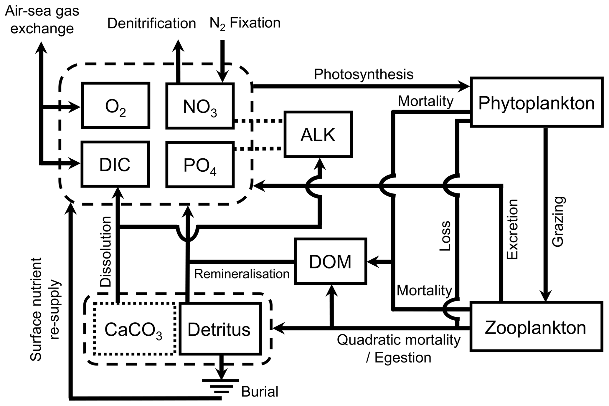
Figure 1Schematic of the ocean biogeochemistry model FOCI-MOPS. Arrows indicate processes and fluxes between model compartments (solid squares). The dashed lines between ALK and NO3 and between ALK and PO4 show that ALK is affected by changes in NO3 and PO4. CaCO3 is represented as a dotted square as it is not a prognostic tracer in the model. See Appendix A for a detailed description. ALK stands for alkalinity, DIC stands for dissolved inorganic carbon, and DOM stands for dissolved organic matter.
For the implementation in FOCI, MOPS has been complemented with a carbon cycle that includes biological uptake and remineralization effects on dissolved inorganic carbon (DIC) and alkalinity (ALK; assuming fixed elemental ratios according to the stoichiometry by Paulmier et al., 2009) and the effects of formation and dissolution of calcite on these two tracers. For biogenic calcite production and dissolution, we implement an implicit approach (Schmittner et al., 2008) where the production of calcite is calculated from organic detritus production in a fixed ratio. Integrated over the entire water column and assuming a fixed molar CaCO3:P ratio from the production of detritus at each time step, the newly produced vertically integrated calcite is then immediately distributed and released as DIC and ALK over the water column with an e-folding length scale. Air–sea gas exchange of CO2 at the sea surface is calculated according to Orr et al. (2017). Altogether, the ocean biogeochemistry is simulated via nine prognostic tracers and five chemical elements (PO4 (P), NO3 (N), O2 (O), DIC (C), ALK (C, N, P), phytoplankton (C, N, P), zooplankton (C, N, P), detritus (C, N, P, Ca), and DOM (C, N, P)).
In MOPS, phytoplankton growth depends on ambient PO4, NO3, temperature, and light. Phytoplankton is grazed by zooplankton and parameterized by a Holling-III function that uses a sigmoidal functional response of the grazing rate to increasing food (Holling and Buckingham, 1976). Subsequent zooplankton egestion and plankton mortality produce sinking detritus and neutrally buoyant DOM. The sinking speed of detritus increases linearly with depth, and the remineralization rate is constant and independent of temperature. In the absence of lateral or vertical exchange, these would result in a flux profile given by a power law of depth (the so-called “Martin” curve with exponent b; Martin et al., 1987). However, the model also simulates oxygen-dependent remineralization of organic matter. If oxygen falls below a threshold, denitrification sets in during anaerobic remineralization and reduces NO3, albeit at a slower rate than aerobic remineralization. The decrease of remineralization caused by oxygen deficiency, especially in oxygen minimum zones, distorts the nominal value of b. There is no benthic denitrification in the model. The loss of fixed nitrogen due to denitrification affects the supply of NO3 to the surface and influences nitrogen fixation at the sea surface, which in the model is diagnosed depending on temperature and the local ratio between simulated NO3 and PO4.
There is no sediment module in MOPS. Organic detritus arriving at the seafloor is partially buried and the burial fraction depends on the rain rate (Appendix A3). The resulting loss of phosphorus and nitrogen to the sediment is compensated for by adding an amount of PO4 and NO3 equivalent to the globally integrated burial, distributed homogeneously in the topmost model layer, rather than through river runoff. Likewise, we account for the burial loss of organic carbon and the associated virtual flux of ALK by a compensating supply of DIC and a decrease of ALK homogeneously distributed over the global sea surface. Supply and removal of these tracers to the surface layer ensures mass conservation with respect to the fluxes across the sea floor. Calcite arriving at the seafloor is not buried but immediately dissolved in the deepest model box, accommodating for the fact that a climate model like FOCI does not allow for the spin-up times needed for CaCO3 sediments to reach a steady state.
With the implementation of MOPS, 1 year of FOCI-MOPS simulation takes 0.6 h and costs about 730 CPU hours with 1260 CPUs (Intel® Xeon® Platinum 9242 Processor) on 14 nodes on the North German Supercomputing Alliance (HLRN) complex LISE at the Zuse Institute Berlin (ZIB). For details of the hardware, please refer to the HLRN-IV documentation on HLRN web page (https://www.hlrn.de/, last access: 10 March 2022). With the same CPU configuration, the computing time for FOCI-MOPS increases by 26 % compared to a physics-only FOCI version. For comparison, an increase of 42 % computing cost was found for the biogeochemical component PISCESv2‐gas implemented in CNRM-ESM2-1 with an online grid-coarsening algorithm (Berthet et al., 2019).
A direct calibration by means of optimization of FOCI-MOPS, a computationally expensive Earth system model (ESM), is presently not feasible. Therefore, we selected MOPS parameters that resulted from a calibration using transport matrices that were derived from a circulation of a reanalysis dataset, the Estimating the Circulation and Climate of the Ocean (ECCO), which is computationally more efficient. In particular, six biogeochemical model parameters of MOPS were adjusted via an automatic calibration procedure against observed nutrient and oxygen distributions as described in Kriest et al. (2020, optimisation ECCO*). While the circulation of the ECCO and FOCI are largely similar, to account for existing differences we manually adjusted three of the six parameters after initial tests as described in Appendix A5. The Appendix also describes the choice of parameters for regulating calcite formation and dissolution. The final full set of parameter values can be found in Table A1.
2.3 Model simulations and data used for model evaluation
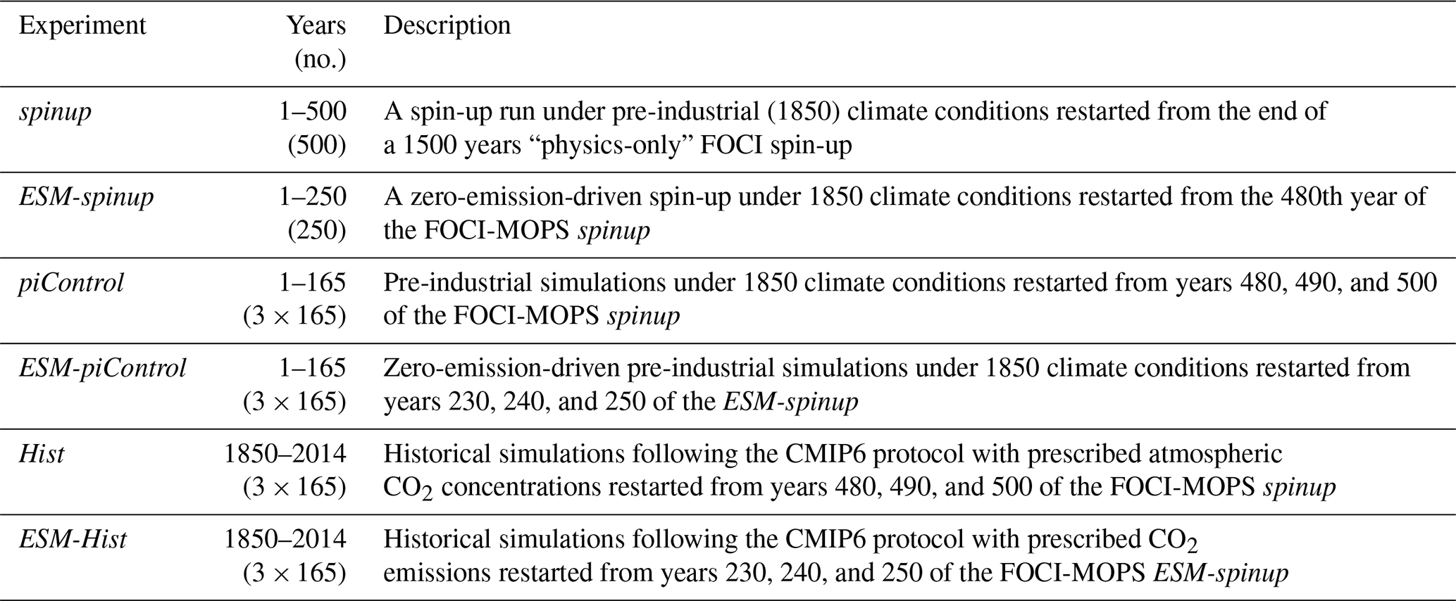
Following the CMIP6 protocol (Eyring et al., 2016), we performed a series of experiments to evaluate FOCI-MOPS (Table 1). A 500-year spin-up with marine biogeochemistry (spinup) was restarted from the end of a 1500-year “physics-only” FOCI spin-up under year 1850 climate conditions (e.g. solar radiation, greenhouse gases, atmospheric nitrogen deposition, sulfate aerosol from volcanic eruptions, land usage, and population density; see Matthes et al., 2020, for details of the boundary conditions.) Details of physical characteristics of the 1500-year spin-up (FOCI1.3-SW038) are described in Matthes et al. (2020), including a cold bias in sea surface temperature (SST) and surface air temperature (SAT) in the North Atlantic and a warm bias in the Southern Ocean. The depth of the maximum transport of the Atlantic meridional overturning circulation (AMOC) is also shallower compared to the RAPID array observations (McCarthy et al., 2015). For the 500-year FOCI-MOPS spin-up, phosphate (PO4), nitrate (NO3), and oxygen (O2) are initialized using the WOA2013 data set (Garcia et al., 2013a, b), and pre-industrial DIC and ALK are taken from GLODAPv2.2016b (Lauvset et al., 2016). The 480th, 490th, and 500th year of the spinup served as different initial conditions for an ensemble of three pre-industrial control (piControl) and transient historical (Hist) simulations (1850–2014) with prescribed atmospheric CO2 concentrations. We also carried out a set of experiments where the model was forced with CO2 emissions and the atmospheric CO2 was calculated prognostically (instead of prescribing atmospheric CO2 concentrations). For those experiments, we use the 480th year of the FOCI-MOPS spin-up as a starting point for a 250-year CO2 zero-emission-driven spin-up (ESM-spinup) to allow for some equilibration between the atmosphere, land, and ocean carbon compartments. An ensemble of three ESM model pre-industrial control (ESM-piControl) and transient historical (ESM-Hist) simulations was then started from the 230th, 240th and 250th year of ESM-spinup.
To evaluate the performance of FOCI-MOPS, we compared the distribution of inorganic tracers in Hist to interpolated and non-interpolated data of GLODAPv2.2016b (Lauvset et al., 2016; Olsen et al., 2016). For O2, NO3, PO4, and ALK, model outputs are averaged over 1972 to 2013, and modelled year 2002 is used for DIC. For organic tracers, 10-year-mean (from 2005 to 2014) chlorophyll estimates from remote sensing (MODIS-Aqua, https://jeodpp.jrc.ec.europa.eu/ftp/public/JRC-OpenData/GMIS/satellite/9km/, last access: 20 January 2021, Melin, 2013), together with in situ observations of mesozooplankton, particulate organic nitrogen, and dissolved organic phosphorus, are used for comparison. Details of the biogeochemical data sets and model evaluation metrics are described in Appendix B.
3.1 Temporal evolution of model simulations
3.1.1 Spin-up drift
Over the first 100 years of the FOCI-MOPS 500-year spin-up (spinup), a small (<1.5 %) decrease in inorganic nutrients (PO4 and NO3) is used to build up organic material (plankton biomass, DOM, and detritus), as they are initialized to zero at the start of spinup. After these initial adjustments, most of the global mean tracer concentrations and globally integrated fluxes showed drifts that were small relative to their mean concentrations (up to 0.1 % in the carbon flux at 2000 m) and reached or asymptotically approached a steady state at the end of spinup (Fig. 2). An exception is NO3 because the marine nitrogen cycle did not reach a steady state, with N2 fixation and denitrification not yet being in equilibrium after 500 years. This is commonly observed in models due to the spatial separation of these counteracting N-cycle processes. The equilibration of marine N2 fixation and denitrification can take thousands of years (Falkowski, 1997; Oschlies et al., 2019). Owing to a net NO3 loss due to a higher global denitrification than N2 fixation rate, together with the build-up of organic matter in the beginning, global-average NO3 is about 1.1 mmol N m−3 lower at the end of the spinup compared to the beginning, amounting to a decrease of 0.007 % per year. After a small positive spike in the beginning, O2 concentrations continuously decrease throughout the spinup and in the end are close to a steady state. The loss of O2 indicates that in the model the supply of O2 via mixing is too slow and/or the consumption due to remineralization is overestimated. The changes in O2 concentration are associated with the temporal drift of the carbon export across 2000 m. While the export flux at 100 m already reached a steady state after 100 years, the flux at 2000 m was still increasing at the end of the spin-up. This reflects that the remineralization of organic matter was slowing down in the upper 2000 m due to the decreasing O2 concentration, allowing an increasing fraction of organic material to remineralize below 2000 m. After 500 years, global-average O2 is about 8.4 mmol O2 m−3 (5 %) lower than in the beginning. In the model, DIC varies mainly due to a build-up of organic matter and changes in air–sea CO2 fluxes. Drift in the DIC inventory during the last 100 years in the spinup is −0.086 Pg C yr−1, which meets the “acceptably small drift” (±0.1 Pg C yr−1) suggested in Jones et al. (2016). Global CaCO3 production equals dissolution as there is no dynamic CaCO3 pool in the model. Therefore, the alkalinity inventory is only affected by the changes in PO4 and NO3. Since PO4 and NO3 decrease during the formation of organic matter and the nitrate reservoir additionally decreases resulting from the imbalance of denitrification and N2 fixation (plus nitrification), the ALK inventory increases during the spinup in the stoichiometric ratio of ALK : NO3 (Paulmier et al., 2009). The remaining small drifts in the spinup might exert an effect on the historical simulations, where they were accounted for by subtracting the respective control simulations.
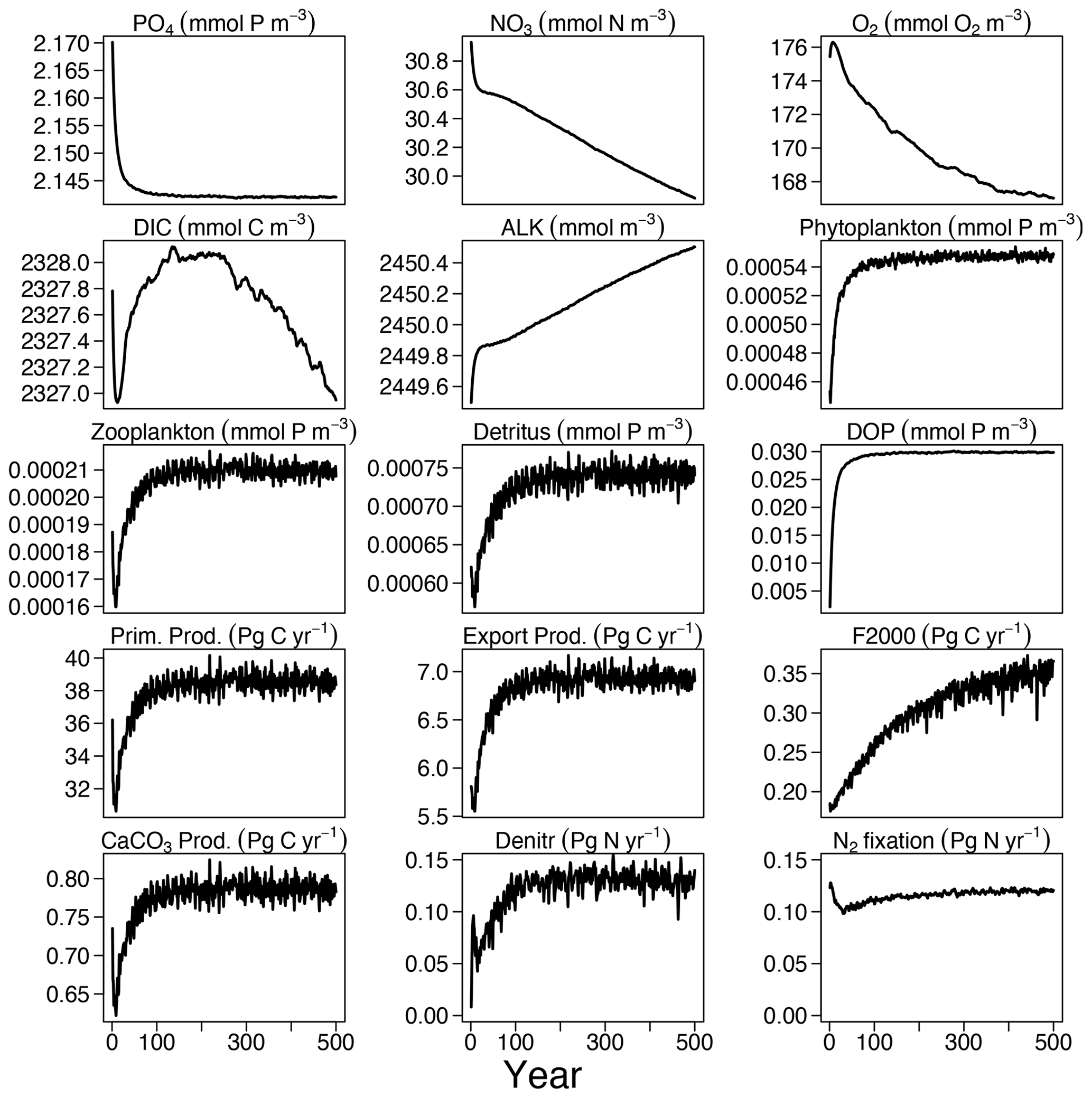
Figure 2Time series of tracer concentrations and fluxes in the 500-year spinup experiment of the inorganic tracers (PO4, NO3, O2, DIC, and ALK), organic tracers (phytoplankton, zooplankton, detritus, and DOP), and fluxes (primary production, export production at 100 m, carbon flux at 2000 m (F2000), CaCo3 production, denitrification (Denitr), and N2 fixation (Nfix)).
3.1.2 Historical simulations
Even after the 500-year spin-up (see Sect. 3.1.1), some drifts in tracers and fluxes can still exist and can been seen in the piControl and ESM-piControl (Figs. S1–S2 in the Supplement). The drifts in Hist and ESM-Hist (Figs. S3–S4) runs are removed by subtracting the piControl and ESM-piControl simulation trends from the corresponding historical runs (Fig. 3). Drifts continue over the additional years of the CO2-emission-driven spin-up (ESM-spinup); therefore, the absolute tracer concentrations and fluxes in ESM-Hist, which is initialized from the end of ESM-spinup, are partly different from those in the Hist runs, as is apparent in the time series of NO3, O2, DIC, and ALK discussed above. Nevertheless, the historical evolution and variability of the ESM-Hist simulation is qualitatively and quantitatively very similar to the one in Hist. In the Hist simulations, PO4 increases slightly, this is mainly due to a decrease in dissolved organic phosphorus (DOP; the model also implicitly represents DOM in phosphorus units in a C : N : P molar ratio of ), which declines by 0.007 % per year. Decreases in phytoplankton, zooplankton, and detritus are also small, ranging from 0.005 % to 0.01 % per year. Global-average NO3 in 2014 is about 0.017 mmol N m−3 (0.06 %) higher than in 1850. One reason for the increase in NO3 is a decrease of denitrification. The reduction of DOM and organic particle pools also contributes to the NO3 increase (0.006 mmol N m−3). The changes in NO3 are also reflected in a decreasing ALK inventory. The simulated relative decrease of the O2 inventory is higher than that of PO4 and NO3. In the model, the ocean loses about 1.5 mmol O2 m−3 (0.9 %) of oxygen between 1850 and 2014. Changes in circulation and mixing, together with the decrease in solubility due to a warming ocean, dominate the decline in marine O2 content. The small decrease in export production would lead to reduced O2 consumption via respiration and therefore elevate rather than reduce the oxygen inventory. Globally averaged DIC increases by 8 mmol C m−3 (0.35 %), mainly due to increased air–sea CO2 fluxes into the ocean under rising atmospheric CO2, i.e. the uptake of anthropogenic CO2.
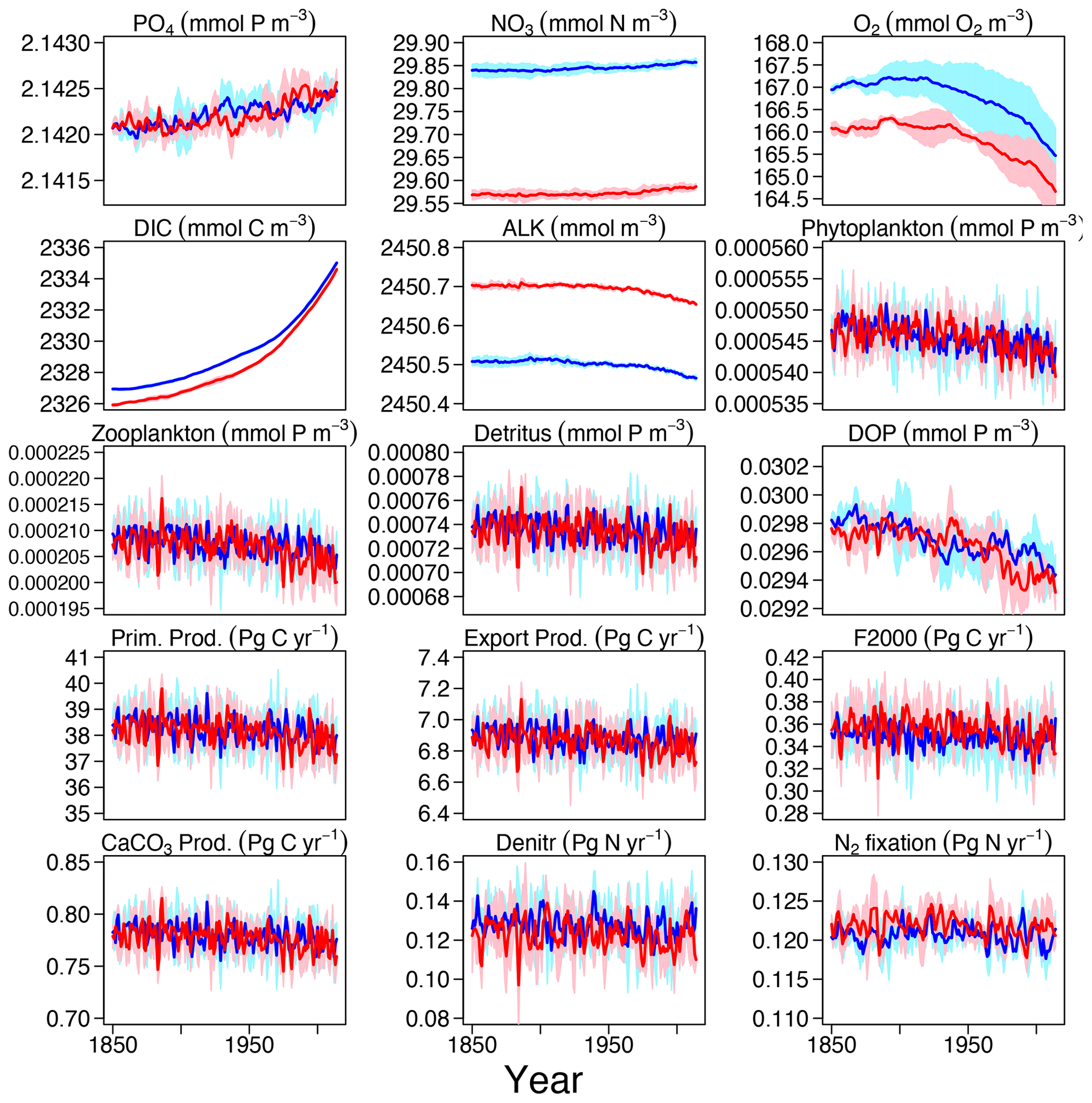
Figure 3Time series of tracer concentrations and fluxes for the 165 years (1850–2014) Hist and ESM-Hist experiments, each for a three-member ensemble. Each ensemble member is corrected by the drifts in the respective piControl and ESM-piControl runs. Dark blue and dark red lines stand for the mean in Hist and ESM-Hist, respectively, and light blue and light red shaded areas represent 1 standard deviation in Hist and ESM-Hist, respectively. The arrangement of the panels is the same as in Fig. 2
3.2 Biogeochemical model performance
3.2.1 Spatial distribution of inorganic tracers
The surface concentration of O2 is primarily determined by the temperature-dependent solubility. In the ocean interior, it is a sensitive balance between ocean circulation and oxygen consumption during remineralization of detritus and dissolved organic matter (DOM). In FOCI-MOPS, water column denitrification occurs in low-oxygen waters when O2 concentration is below 36 mmol O2 m−3. The low-oxygen waters develop where the physical supply of O2 is sluggish and O2 consumption via respiration is high. The model reproduces the low-oxygen waters at the eastern margins of tropical and subtropical ocean basins (Figs. 4a and S5). In the zonally averaged ocean basin means, the low-oxygen waters are situated between 100 and 1500 m in the Atlantic, Indian, and Pacific oceans (Fig. 4a and d–f). In the same depth range, the modelled O2 is biased low, particularly in the Southern Hemisphere (Figs. 4i–k and S5). Another region with clear negative O2 biases can be seen at depths below 1500 m and all the way to the bottom in the Pacific Ocean (Fig. 4k). The low biases in the zonal mean are due to an underestimated O2 in the eastern equatorial Pacific (Fig. S5), a feature that is likely due to overestimated production in the euphotic zone above and imperfect physics and remineralization settings, which are commonly found in numerical models (Dietze and Loeptien, 2013; Ilyina et al., 2013; Cabré et al., 2015; Paulsen et al., 2018). In general, O2 in the model is biased high between 1000 and 3000 m and is biased low below 3000 m. In addition to the biological processes, the difference can be explained by the ventilation of the water masses. The modelled AMOC has a shallow bias and is indeed weaker in the deep water (3000–5000 m; Fig. 5), as also remarked upon in Matthes et al. (2020) and common across climate models (e.g. Weijer et al., 2020). A more sluggishly ventilated deep water in latitude–depth structure (Fig. 5a) is consistent with the higher concentration in inorganic tracers and the negative biases in O2.
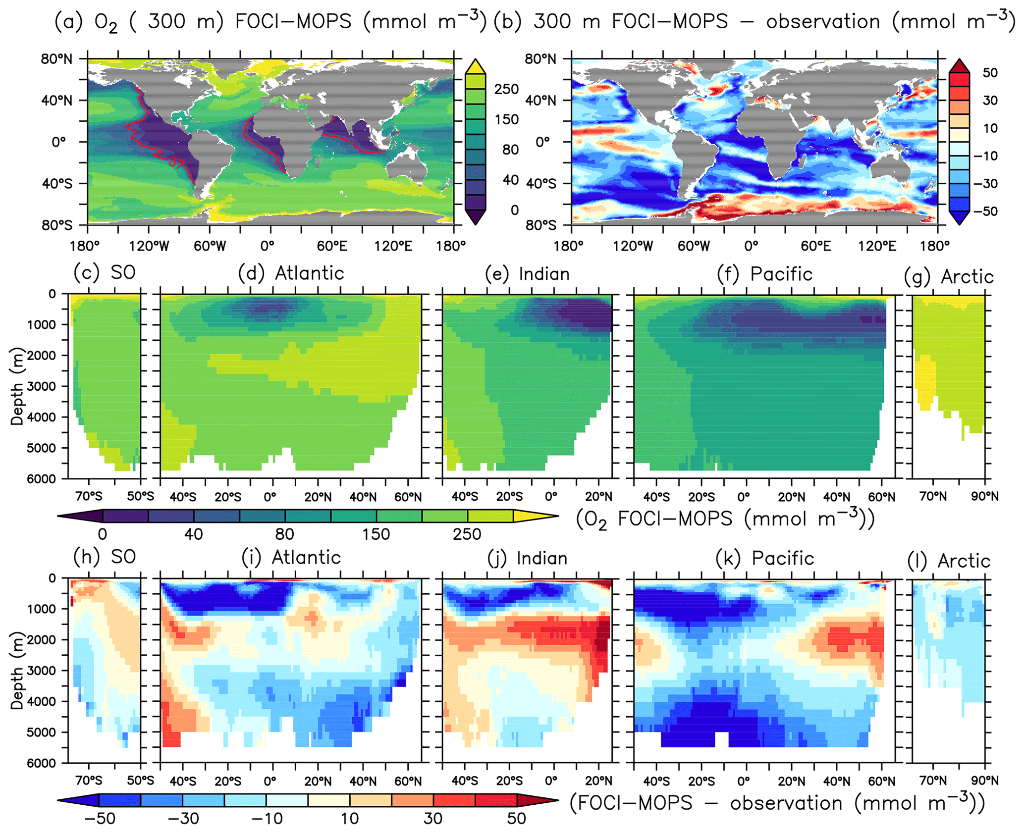
Figure 4O2 climatology over 1972–2013 of the Hist simulations at (a) 300 m depth and zonally averaged across the (c) Southern, (d) Atlantic, (e) Indian, (f) Pacific, and (g) Arctic oceans in FOCI-MOPS. The corresponding difference of model minus observation are shown in (b) and (h)–(l), respectively. Observational data are from GLODAPv2.2016b, which covers 1972–2013 (Lauvset et al., 2016; Olsen et al., 2016). Red contour lines in (a) depict O2 of 36 mmol O2 m−3, below this concentration anaerobic remineralization kicks in in the model. Partitioning of ocean basins follows the World Ocean Atlas 2013 definitions.
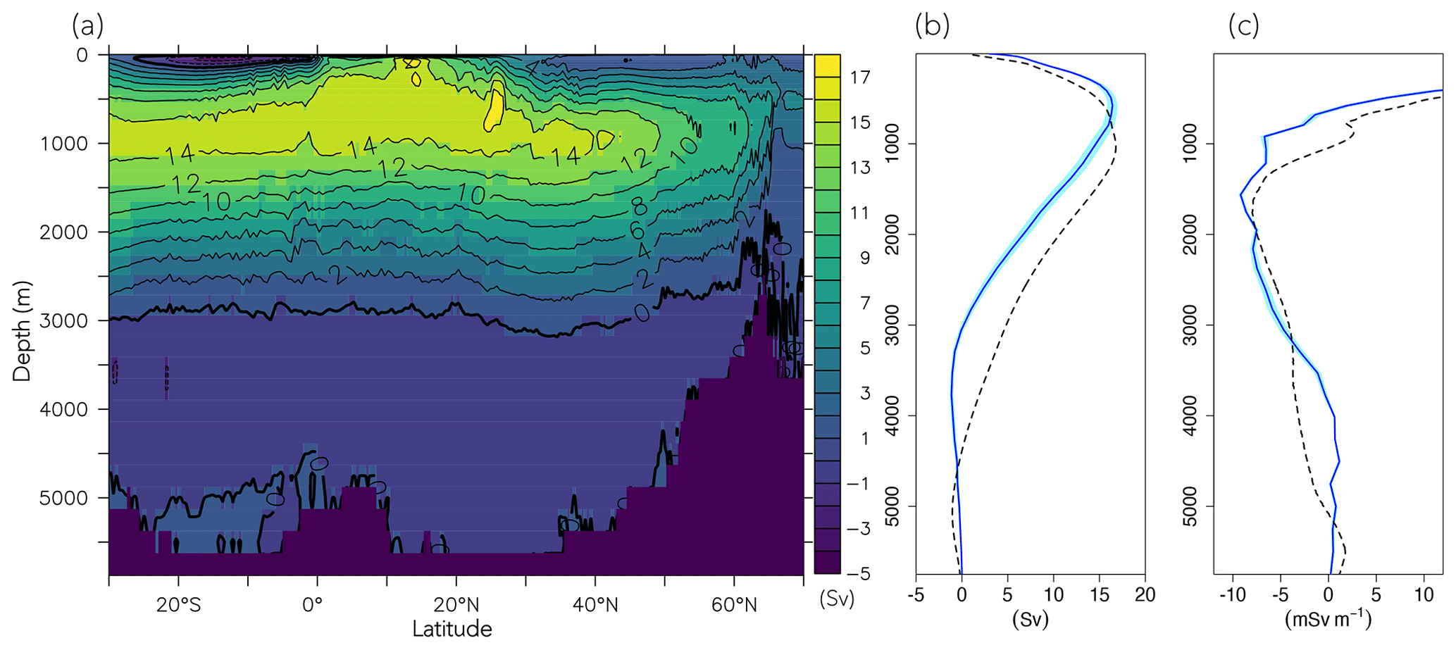
Figure 5Atlantic meridional overturning stream function climatology over 2004–2014 of the Hist simulations. (a) Latitude–depth structure, (b) vertical profile at 26.5∘ N, and (c) z derivative of AMOC at 26.5∘ N. Blue lines and the shaded areas are modelled results, and dashed black lines are observational values from the RAPID array (McCarthy et al., 2015).
Surface phosphate (PO4) concentrations simulated by FOCI-MOPS generally agree with observations, with positive biases in the Atlantic and a negative bias in the subarctic gyre in the northern Pacific Ocean (Fig. 6a and b). In the interior, the model–data misfits are generally smallest in the Southern Ocean (SO) and the Arctic (Fig. 6h and l). In the Atlantic, Indian, and Pacific oceans, modelled PO4 shows positive biases at around 100–1000 m and below 3000 m and negative biases between 1000 and 3000 m (Fig. 6i–k).
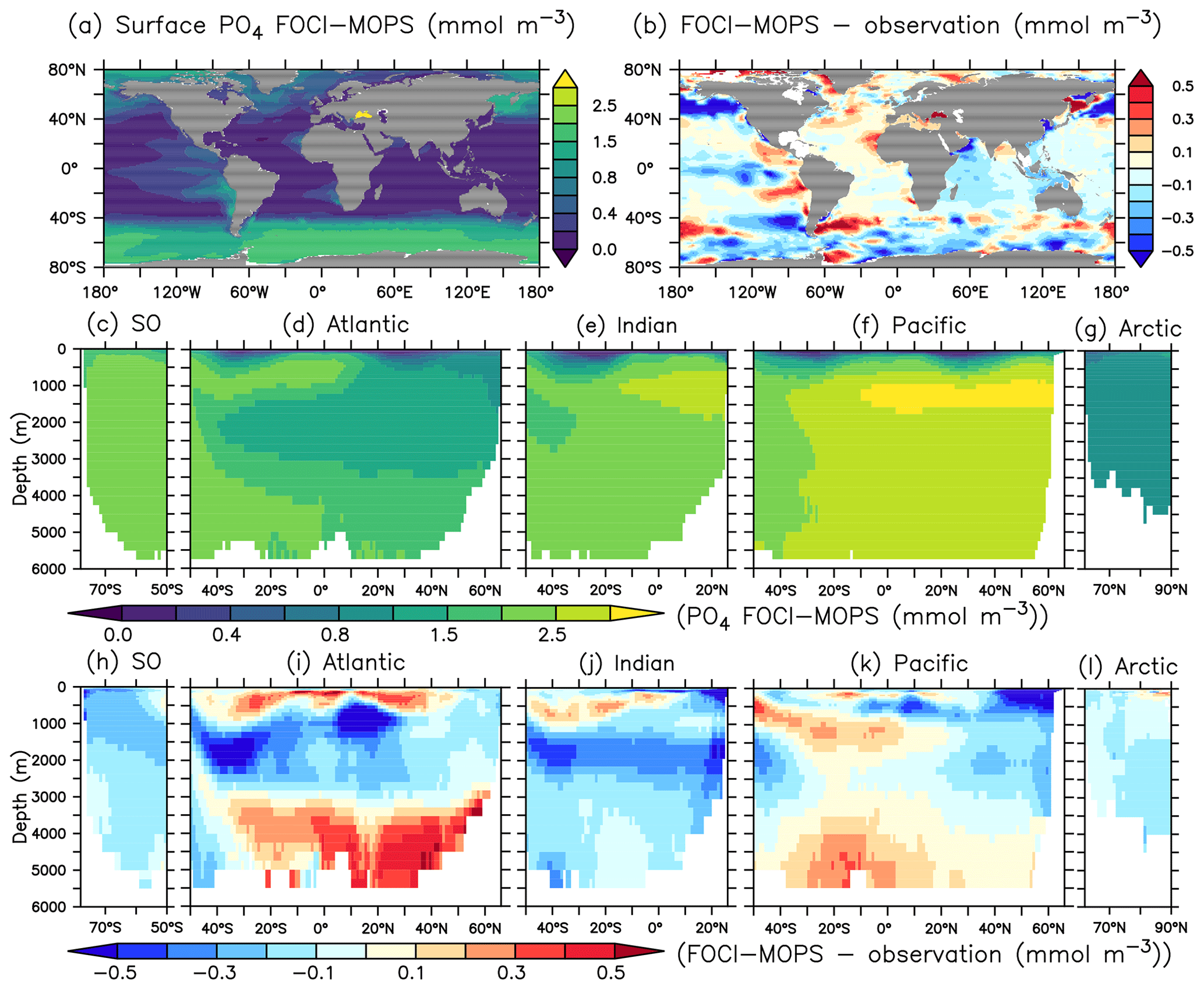
Figure 6PO4 climatology over 1972–2013 of the Hist simulations (a, c–g) and the model–observation difference (b, h–i). Observational data are from GLODAPv2.2016b, which covers 1972–2013 (Lauvset et al., 2016; Olsen et al., 2016). The order of the panels is the same as in Fig. 4.
In order to better understand the distribution of PO4, we adopt the methodology of Duteil et al. (2012) and calculate regenerated (PO) and preformed PO4 (PO) assuming oxygen saturation (O) at isopycnal outcrops (e.g. PO AOUO2: PO4, AOU = O O, PO PO4−PO). For observations, we apply the O2: PO4 ratio of 170 mol O2: mol P estimated in Anderson and Sarmiento (1994). For model output, we apply the ratio of 165.08044 mol O2: mol P used in the model.
Except for the deep Atlantic (deeper than 3000 m), preformed PO4 is generally too low in the ocean interior compared to observations (Fig. 7h–k). A lack of iron limitation in the model could cause a too strong uptake of PO4 by phytoplankton in iron-limited regions, such as the Southern Ocean, and lead to too low preformed PO4. The overestimated regenerated PO4 in the deep Pacific >3000 m (Fig. 8k) contributes to the overall high bias of PO4 (Fig. 6k) and is consistent with the low O2 biases in the same region (Figs. 4k and S5). The high bias of PO4 may be at least partly explained by excessive remineralization of detritus and DOM in the eastern Pacific Ocean as a result of overestimated primary production (PP) and export production (EP; see Sect. 3.3). A too sluggish ventilation of these water masses could also explain the excessive accumulation of regenerated PO4 and apparent oxygen utilization (Fig. 5), as the PO4 is also overestimated in the deep Atlantic Ocean.
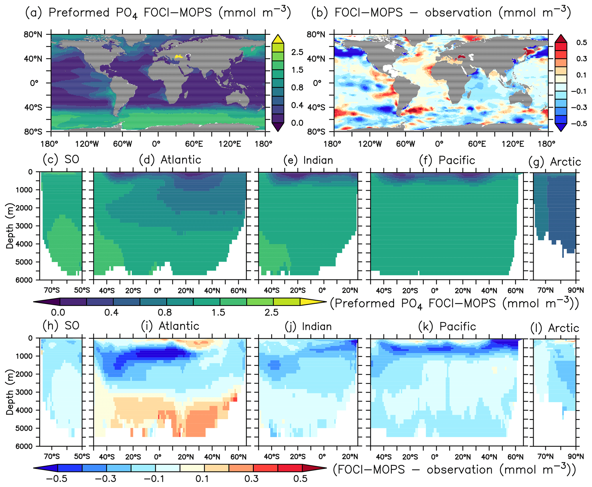
Figure 7Preformed PO4 climatology over 1972–2013 of the Hist simulations (a, c–g) and the difference with observations using GLODAPv2.2016b, which covers 1972–2013 (Lauvset et al., 2016; Olsen et al., 2016) (b, h–i). Preformed PO4 is estimated as PO4 minus regenerated PO4. The order of the panels is the same as in Fig. 4.
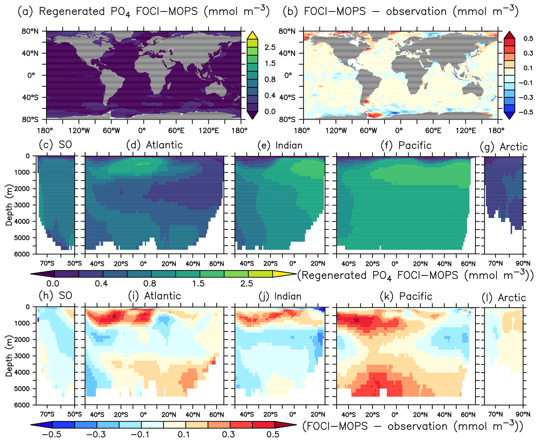
Figure 8Regenerated PO4 climatology over 1972–2013 of the Hist simulations (a, c–g) and the difference with observations using GLODAPv2.2016b, which covers 1972–2013 (Lauvset et al., 2016; Olsen et al., 2016) (b, h–i). Regenerated PO4 is estimated as apparent oxygen utilization; see text. The order of the panels is the same as in Fig. 4.
Biases of climatological nitrate NO3 overall show a similar distribution as for phosphate (Fig. 9a). Simulated NO3 differs from the pattern of PO4 mostly in low latitudes at intermediate depth. Some positive biases can be seen in the Arctic and near the Southern Hemispheric Subtropical Front (Fig. 9b). In the ocean interior, NO3 is removed by denitrification. Substantial rates of denitrification can be realized (depending on the supply of organic matter) when O2 concentrations fall below a few mmol m−3 (Eqs. A11 and A16). Modelled denitrification occurs in the Atlantic Ocean, the northern Indian Ocean, and the eastern tropical Pacific Ocean and is most prominent in the Pacific Ocean (black contour lines in Fig. 9i–k). Globally integrated water column denitrification in the model amounts to 0.13 Pg N yr−1, higher than observation-based estimates (ranging from 0.02 to 0.12 Pg N yr−1; see Sect. 3.3 below). It is likely that excessive denitrification contributes to some of the negative biases between 300 and 1000 m in the low-latitude oceans (Figs. 9i–k and S5) that are not accompanied by similar negative biases in PO4 (Fig. 6i–k).

Figure 9NO3 climatology over 1972–2013 of the Hist simulations and the difference model-observation. Black contour lines represent zonally integrated denitrification rates (mmol N m−2 d−1). Observational data are from GLODAPv2.2016b, which covers 1972–2013 (Lauvset et al., 2016; Olsen et al., 2016). Panels are ordered as in Fig. 4.
The spatial pattern of dissolved inorganic carbon (DIC) and alkalinity (ALK) in general agree with observed patterns at the sea surface, but both show negative biases (Figs. 10b and 11b). In the interior, the biases turn positive below 3000 m for both DIC and ALK, which is most obvious in the Atlantic and the Pacific Oceans, similar to the patterns of PO4 and NO3. In the ocean, potential differences in CO2 uptake between model and observations can contribute to DIC biases. Both DIC and ALK are affected by the remineralization of detritus and the production of CaCO3, via zooplankton egestion and plankton mortality in the surface layer and dissolution of CaCO3 throughout the water column, respectively. There is a clear transition from a negative bias of DIC and ALK in the surface ocean to a positive bias in deep waters across all ocean basins, except the Arctic where plankton activity is limited (Fig. 11h–l). This indicates that the e-folding export and dissolution of CaCO3 (Sect. A2.2) might lead to an excessive transport of ALK (and DIC) to the deep ocean. The positive biases in DIC and ALK in the deep water might also indicate a too sluggish ventilation of deep waters, which is also consistent with the positive biases in PO4 and NO3, as well as the negative bias in O2.
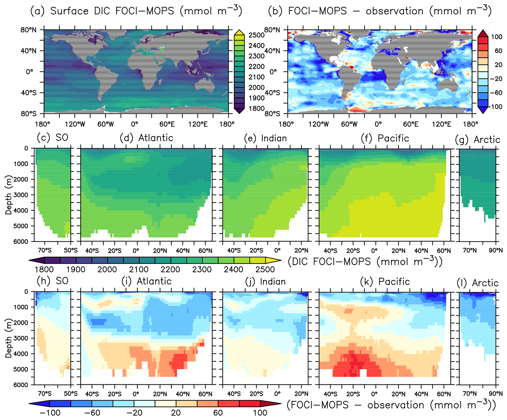
Figure 10Dissolved inorganic carbon (DIC) for the year 2002 in the Hist simulations and the model–observation difference. Observational data are sum of the preindustrial TCO2 and the accumulated anthropogenic carbon in the year 2002 from GLODAPv2.2016b (Lauvset et al., 2016; Olsen et al., 2016). The order of panels is the same as in Fig. 4.
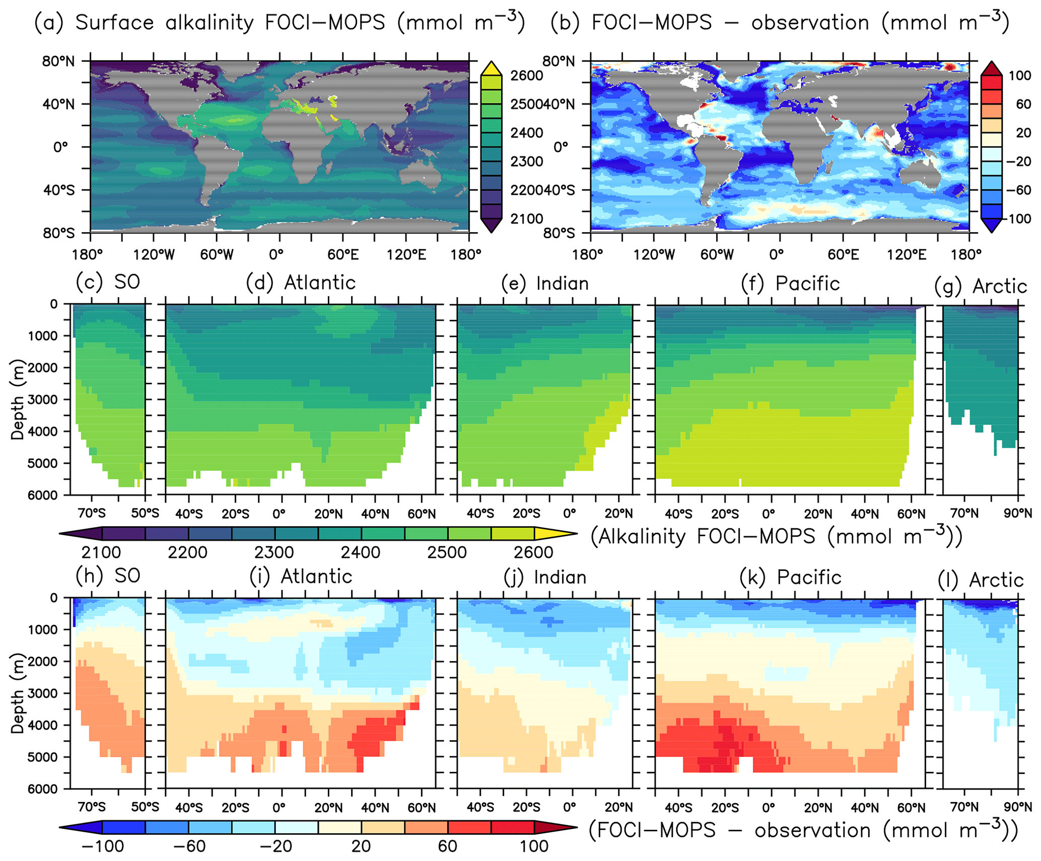
Figure 11Alkalinity (ALK) climatology over 1972–2013 in the Hist simulations and the model–observations difference. Observational data are from GLODAPv2.2016b, which covers 1972–2013 (Lauvset et al., 2016; Olsen et al., 2016). The order of panels is the same as in Fig. 4.
Typically, 1 standard deviation of distribution of the inorganic tracers is smaller than 10 % of the mean value of the Hist ensemble simulations (Figs. S6–S12). Areas with higher variation usually occur where vertical mixing is stronger, such as at high latitudes.
3.2.2 Spatial distribution of organic tracers in the surface
In FOCI-MOPS, the growth of phytoplankton is determined by temperature, light, and ambient NO3 and PO4 concentrations (Eqs. A1–A5). The distribution of phytoplankton (Phy) in the surface layer (∼6 m) overall agrees relatively well with observational estimates (Fig. 12a, e, and i), the most distinct discrepancies occur in coastal regions, where the observed phytoplankton concentrations often exceed 0.06 mmol P m−3 but modelled phytoplankton do not (Fig. 12e). The difference might be due to the lack of terrestrial nutrient runoff in the current model version. In addition, shelves are not well resolved with a spatial resolution, a typical bias of global models. In the open-ocean pelagic regions, however, the modelled phytoplankton is usually higher than the observations, which might be due to the missing iron limitation in the model. The higher phytoplankton biomass might also explain some of the low biases in PO4 in the equatorial regions.

Figure 12Organic tracer concentrations for the first layer (∼6 m) of phytoplankton (Phy), 0–100 m of zooplankton (Zoo), particulate organic phosphorus (POP), and dissolved organic phosphorus (DOP) climatology over 2005–2014 in the Hist simulations (a–d), observations (e–h), and the zonally averaged values (i–l). In the zonally averaged panels, model results are subsampled according to the availability of observations. Observational data of Phy, Zoo, and POP are derived from chlorophyll (MODIS-Aqua; Melin, 2013), mesozooplankton (MAREDAT; Moriarty and O'Brien, 2013), and POM (Martiny et al., 2014), respectively. Observations of DOP are from multiple published (Torres-Valdés et al., 2009; Moutin et al., 2008; Landolfi et al., 2016; Yoshimura et al., 2007) and unpublished (Landolfi, unpublished) data sets. See Sects. B2.2, B2.3, B2.4, and B2.5 for details of the observations.
Zooplankton and particulate organic phosphorus (POP, sum of simulated phosphorus in detritus, phytoplankton, plus half of the zooplankton; see Sect. B2.4 for further details) are generally closely associated with the presence of phytoplankton; their distributions largely correlate with those of phytoplankton in the model (Fig. 12b and c). While the large-scale pattern is similar, Zooplankton and POP are less homogeneously distributed than phytoplankton. For example, modelled phytoplankton biomass is around 3-fold greater in the nutrient-replete eastern tropical Pacific than in the oligotrophic gyres, while the same ratio can be over 10-fold for zooplankton. Modelled zooplankton are overestimated around the Equator and the Southern Ocean around 40∘ S in the surface (0–100 m; Fig. 12j), where phytoplankton is also overestimated (Fig. 12i). Observations show much higher POP at high latitudes than low latitudes at the surface (0–100 m; Fig. 12k), which is not captured by the model. Note that observational data of phytoplankton, zooplankton, and POP are from different types of estimates; therefore, the observations do not necessarily correlate to each other as in the model. As dissolved organic phosphorus (DOP) is neutrally buoyant, it is controlled by ocean circulation in addition to the production and remineralization. DOP is much lower in the deeper water than at the surface; therefore, in upwelling regions such as the eastern equatorial Pacific, DOP is lower. Meanwhile, nutrient supply from the upwelling promotes the growth of phytoplankton and the production of POP. As a result, the spatial distribution of surface DOP in the model in general is negatively correlated with POP and is more homogeneously distributed (Fig. 12d). Observations of DOP are very sparse but suggest that DOP tends to be overestimated in the model. This may indicate a too long DOP remineralization timescale; however, a shorter timescale may lead to an even stronger bias in surface phosphate concentrations (Fig. 12). Alternatively, changing the partitioning between DOP and POP production (e.g., via parameter σDOP in Eqs. A9 and A10), together with modified POP sinking speed and remineralization could potentially improve DOP without negative effects on other (surface) components. Further investigations regarding the simultaneous fit of MOPS to all inorganic and organic tracers are currently underway.
Similar to the inorganic tracers, 1 standard deviation of distribution of the organic tracers is smaller than 10 % of the mean value of the Hist ensemble simulations (Fig. S13).
3.2.3 Statistical performance of the simulated inorganic and organic tracers
The correlation coefficient r, standard deviation σM, and centred root-mean-squared error (RMSE′, RMSE minus global bias) of modelled nutrients and oxygen show a very good match compared to the non-interpolated observations (Table 2, Fig. 13), although nutrients are biased somewhat low, especially at the surface (0–100 m), which is the only depth range where oxygen shows a high bias (note the shading of symbols in Fig. 13). The modelled ALK and DIC are biased slightly low above 2000 m. The modelled surface ALK averaged over 1972 to 2013 is 2286±1 mmol m−3, and surface DIC averaged over 1870 to 1899 (pre-industrial DIC) is 1985±0 mmol m−3. They are lower than the values among CMIP5 models (surface ALK and pre-industrial DIC are 2365–2500 and 2050–2170 mmol m−3, respectively; Oka, 2020) but are only slightly lower than the observations (surface ALK and pre-industrial DIC are 2362 and 2019 mmol m−3, respectively; Lauvset et al., 2016; Olsen et al., 2016). Note that the low bias in the full-domain ALK here is contrary to a higher inventory when compared to the initial state (Figs. 2 and 3). The low bias against individual (non-interpolated) data results from the fact that more observations are located in the upper 2000 m, where the model underestimates ALK concentrations. Compared to global model assessments of CMIP5 models with similar metrics evaluated by Ilyina et al. (2013), Séférian et al. (2013), and Kwiatkowski et al. (2014), the model performs well (Table 2) with respect to dissolved inorganic tracers.
Table 2Correlation coefficient r, normalized standard deviation , global bias normalized by observed mean (in squared brackets the non-normalized bias is shown, given in µg Chl L−1 for phytoplankton and in mmol m−3 for all other tracers), and Bhattacharyya distance (BD) of experiment Hist presented in this study and from studies by Ilyina et al. (2013, historical run in “MR” model configuration, Table 5; “I2013”), Séférian et al. (2013, one biogeochemical model with three different circulations, Table 3; “S2013”) and Kwiatkowski et al. (2014, six biogeochemical models in one circulation, Table 3; “K2014”). Except for chlorophyll, the values in FOCI-MOPS are from comparison with non-interpolated data from GLODAPv2.2016b (Lauvset et al., 2016; Olsen et al., 2016). Round brackets are introduced for distinguishing hyphen and negative signs. For all model studies we report metrics for the surface (here refers to 0–100 m); additionally, for the metrics by Ilyina et al. (2013) we show the range over five different depth levels (surface, 100, 500, 1000, and 3000 m) in the “all domains” column. For the all domains column in this study we show the range over seven different vertical domains (0–100, 100–200, 200–500, 500–1000, 1000–2000, 2000–5000, 0–8000 m). For metrics by Séférian et al. (2013), we report the range over three different circulations and for metrics by Kwiatkowski et al. (2014) the range over five different models is reported. Note that, except for the Bhattacharyya distance, all metrics of Hist have been calculated from volume-weighted properties.
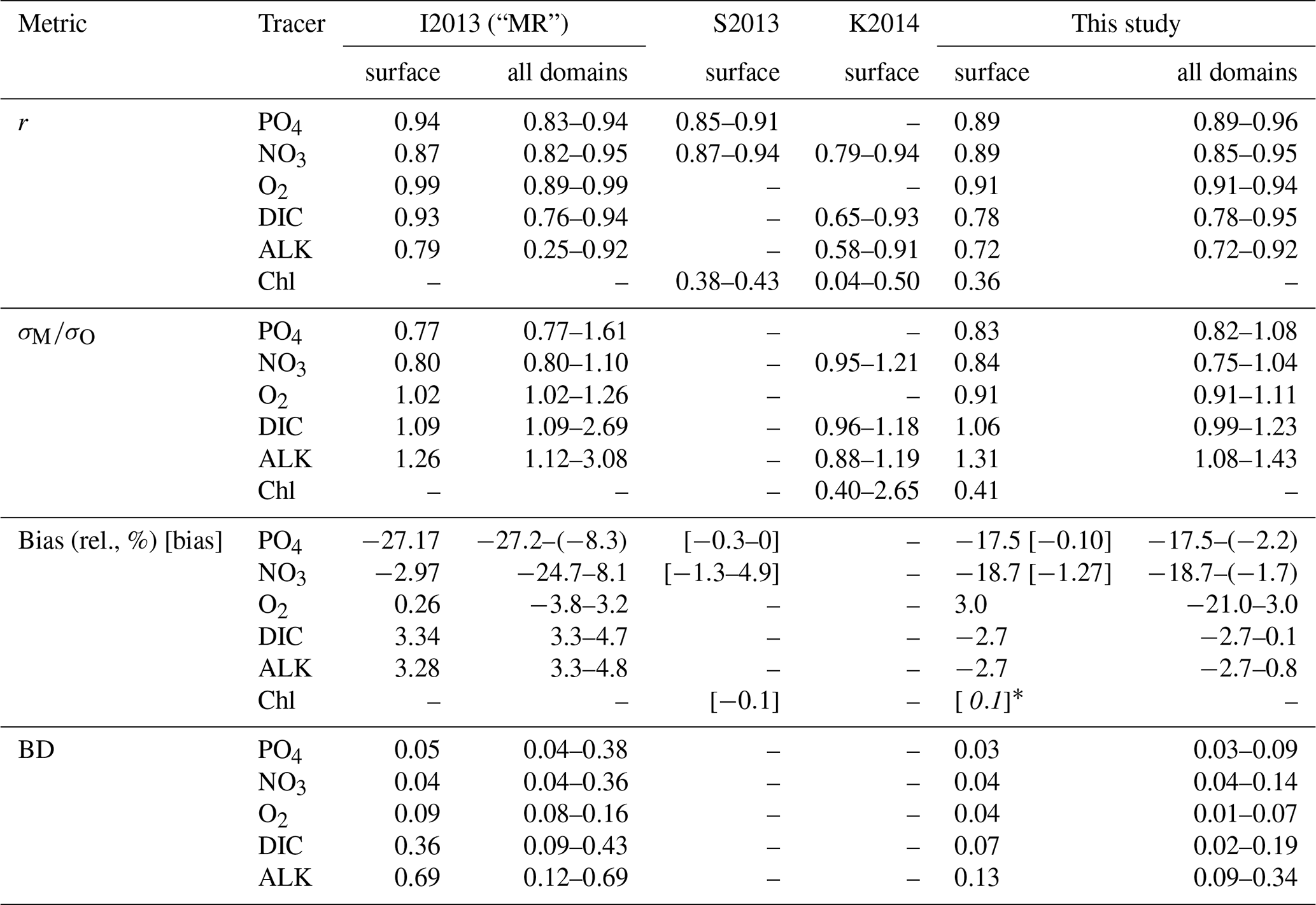
* Computed from phosphorus units via a C : Chl according to Sathyendranath et al. (2009).
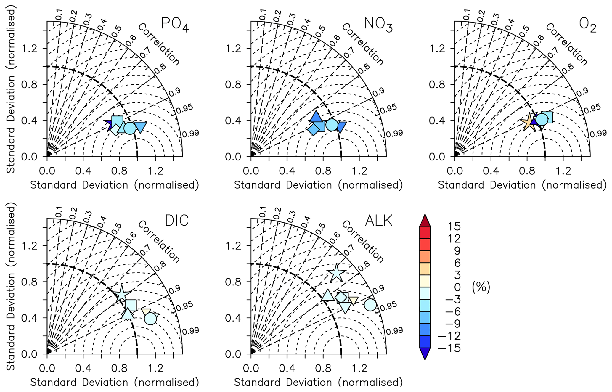
Figure 13Taylor diagrams for phosphate (PO4), nitrate (NO3), oxygen (O2), dissolved inorganic carbon (DIC), and alkalinity (ALK) (left to right). Colours indicate model bias (relative to observations; in percent). The model is subsampled according to the availability of observations. Observational data are from GLODAPv2.2016b (Lauvset et al., 2016; Olsen et al., 2016). Symbols indicate different vertical domains: star indicates 0–100 m, square indicates 100–200 m, diamond indicates 200–500 m, triangle indicates 500–1000 m, delta indicates 1000–2000 m, small delta indicates 2000–5000 m, and circle indicates full domain.
The model fit worsens for the organic tracers, with a correlation coefficient between 0.11 (DOP) and 0.42 (POP), and generally a too low spatial variance (between 41 and 61 % of the observations; Table B2 and Fig. 14). Except for POP, organic tracers are biased high, and RMSE and RMSE′ are large. Thus, the statistical metrics indicate a lower performance of the model for the organic tracers chlorophyll, zooplankton, DOP, and POP. Nevertheless, the results for phytoplankton and chlorophyll are in line with earlier global model studies (Table 2). Note also that the uncertainty of the observational estimates of organic tracers is larger compared to inorganic tracers, the in situ observations are sparse in space and time, with sampling biases, e.g., towards summer and with less high-latitude observations (see also Appendix B2.).
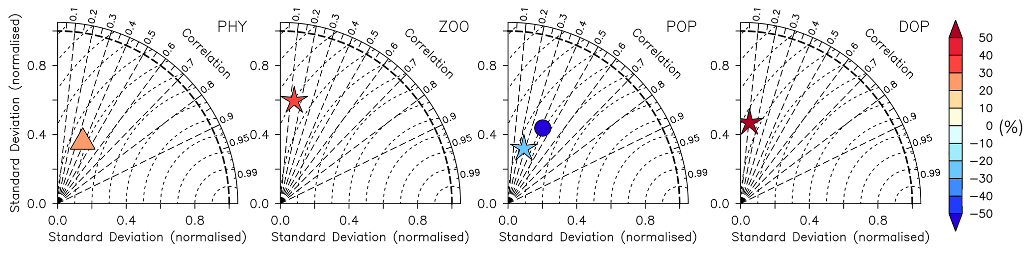
Figure 14Taylor diagrams for phytoplankton (PHY), zooplankton (ZOO), particulate organic phosphorus (POP), and dissolved organic phosphorus (DOP) as shown in Fig. 12 (left to right). Colours indicate model bias (relative to observations; in percent). Observational data of Phy, Zoo, and POP are derived from chlorophyll (MODIS-Aqua; Melin, 2013), mesozooplankton (MAREDAT; Moriarty and O'Brien, 2013), and POM (Martiny et al., 2014), respectively. Observations of DOP are from multiple published (Torres-Valdés et al., 2009; Moutin et al., 2008; Landolfi et al., 2016; Yoshimura et al., 2007) and unpublished (Landolfi, unpublished) data sets. See Sects. B2.2, B2.3, B2.4, and B2.5 for details of the observations. The model is subsampled according to the availability of observations. Symbols indicate different vertical domains: triangle indicates surface (∼6 m), star indicates 0–100 m, and circle indicates full domain (POP only).
Even if a biogeochemical model component is dynamically correct, a slight distortion in the physical model (e.g. a slight spatial shift in ocean current) can cause a large RMSE and thereby induce a large model error. To account for such effects we have calculated three metrics that do not rely on the exact spatial pattern of tracers, but on the concentration distribution, namely the Bhattacharyya distance (BD, Bhattacharyya, 1946), which evaluates the similarity between observed and simulated frequency distributions of tracers, the Hellinger distance (HD, Hellinger, 1909), which is related to BD via BD , and the L1 norm, which evaluates the absolute difference between observed and simulated distributions. For all three metrics, smaller model–data misfit is associated with larger area of overlap between the two distributions, which yields smaller values (see Appendix B3). Figures 15 and 16 show examples for the distributions of inorganic and organic tracers, and Table B2 lists the metrics for different tracers. Applying these metrics, it is evident that most organic tracers (phytoplankton, zooplankton, and POP), despite suffering from a large error with respect to r and RMSE, in general reflect the observed distribution (Fig. 16), and they thus exhibit values for, e.g., BD, that are in the same range as those of inorganic tracers. Only the strong overestimate of DOP by the model is also reflected in BD. Here the model shows a much higher misfit than for any other tracers for all metrics.
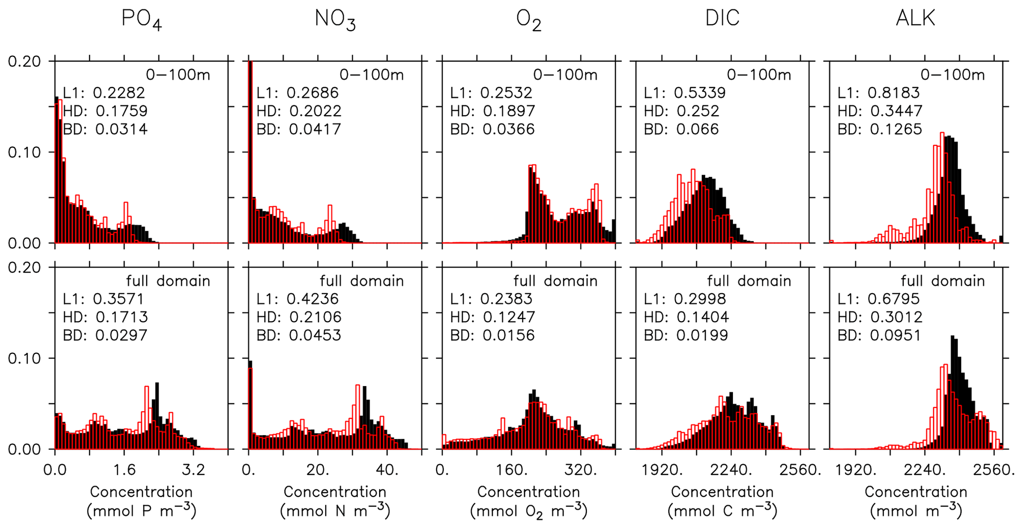
Figure 15Frequency distribution of phosphate (PO4), nitrate (NO3), oxygen (O2), DIC, and alkalinity (left to right) from observations (filled black bars) and model (red bars) for the surface (0100 m, top) and the full model domain (bottom). Numbers denote three different metrics for the similarity of the distributions, namely L1 (Eq. B3), HD (Eq. B2), and BD (Eq. B1). Observational data are from GLODAPv2.2016b. The data cover 1972–2013. except for DIC, which represents for the year 2002 (Lauvset et al., 2016; Olsen et al., 2016).
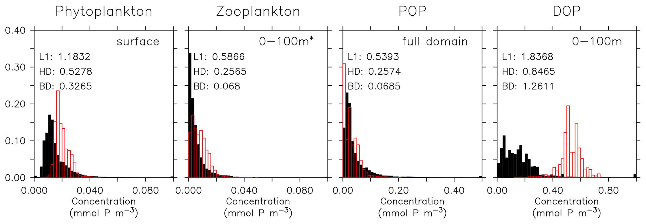
Figure 16Frequency distribution of surface phytoplankton, zooplankton (0–100 m), POP (full domain), and DOP (0–100 m). Observational data of Phy, Zoo, and POP are derived from chlorophyll (MODIS-Aqua; Melin, 2013), mesozooplankton (MAREDAT; Moriarty and O'Brien, 2013), and POM (Martiny et al., 2014), respectively. Observations of DOP are from multiple published (Torres-Valdés et al., 2009; Moutin et al., 2008; Landolfi et al., 2016; Yoshimura et al., 2007) and unpublished (Landolfi, unpublished) data sets. See Sects. B2.2, B2.3, B2.4, and B2.5 for details of the observations. The model is subsampled according to the availability of observations. Colours and numbers are as described in Fig. 15.
To summarize, in terms of tracer distributions the performance of MOPS in FOCI is comparable to other global models and even generally better with respect to inorganic tracers. The fit deteriorates with regard to the organic components in the cases of plankton and POP and has a high bias for DOP.
3.3 Globally integrated biogeochemical fluxes and their spatial patterns
3.3.1 Oceanic biogeochemical fluxes
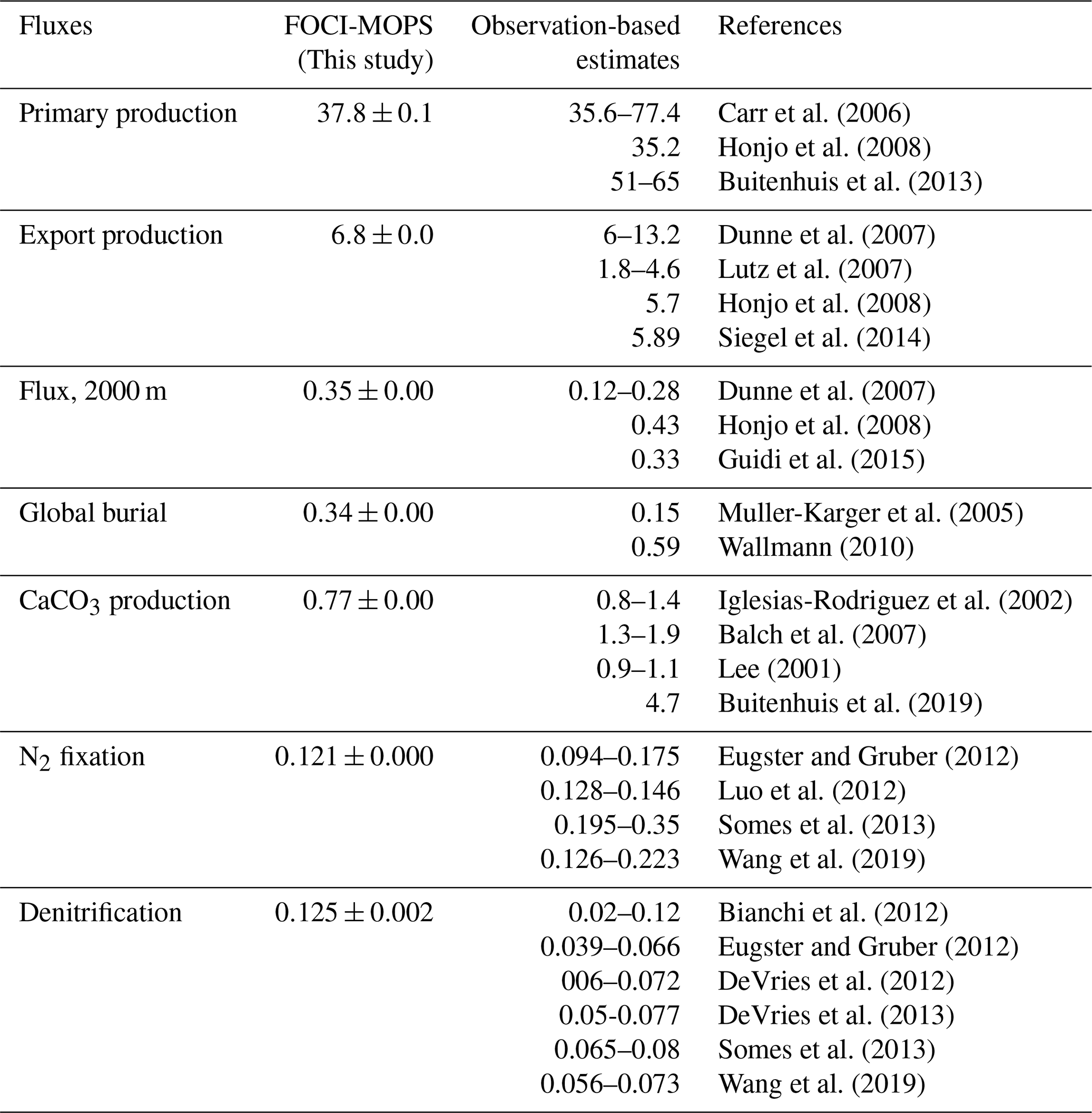
We average the globally integrated biogeochemical fluxes simulated by FOCI-MOPS over the time period 2005 to 2014 and over the ensemble of three Hist simulations (Table 3). Overall, primary production (37.8 Pg C yr−1), export production, the sinking of detritus at 100 m (6.8 Pg C yr−1), the flux of detritus at 2000 m (0.35 Pg C yr−1), burial of detritus that sank to the bottom of the ocean (0.34 Pg C yr−1), and N2 fixation (0.12 Pg N yr−1) are within the range of observation-based estimates. CaCO3 production (0.77 Pg C yr−1) is lower than previous observation-based estimates (0.8–4.7 Pg C yr−1). Water column denitrification (0.13 Pg N yr−1) is slightly higher than observational estimates.
Carr et al. (2006)Honjo et al. (2008)Buitenhuis et al. (2013)Dunne et al. (2007)Lutz et al. (2007)Honjo et al. (2008)Siegel et al. (2014)Dunne et al. (2007)Honjo et al. (2008)Guidi et al. (2015)Muller-Karger et al. (2005)Wallmann (2010)Iglesias-Rodriguez et al. (2002)Balch et al. (2007)Lee (2001)Buitenhuis et al. (2019)Eugster and Gruber (2012)Luo et al. (2012)Somes et al. (2013)Wang et al. (2019)Bianchi et al. (2012)Eugster and Gruber (2012)DeVries et al. (2012)DeVries et al. (2013)Somes et al. (2013)Wang et al. (2019)Table 3Primary production, export production, flux of detritus at 2000 m, global burial, CaCO3 production (Pg C yr−1), N2 fixation, and water column denitrification (Pg N, yr−1) in Hist simulations (averaged over 2005–2014) and observation-based estimates.
The highest annual primary production occurs in the eastern equatorial Pacific Ocean and some coastal regions (>1000 mg C m−2 d−1, Fig. 17a). In the subtropical oligotrophic gyres, it is typically lower than 200 mg C m−2 d−1. The spatial distributions of export production at 100 m and CaCO3 production (Fig. 17b and c) are similar to that of primary production, suggesting that the latter is largely driving the former. The spatial pattern of the flux of sinking detritus at 2000 m is less similar to that of primary production due to the effects of advection and mixing (Fig. 17d). The distinct high flux at 2000 m depth in the eastern Pacific is partly due to the low O2 levels between the surface and 2000 m depth mentioned earlier. Regions of elevated flux of detritus largely overlap with O2 concentrations below 36 mmol O2 m−3, which is the threshold for anaerobic remineralization in the model. Denitrification is shaped by low O2 levels associated with high primary production, consequent detritus flux, and sluggish ventilation, particularly in the so-called shadow zones along the eastern margins of the subtropical oceans (Fig. 17e). These biological and physical effects together result in the most pronounced water column denitrification in the eastern tropical Pacific, which accounts for 71 % of the global denitrification rate in our model, which is within the range that was derived from nitrogen gas measurements (70 %–88 %; DeVries et al., 2012). Due to temperature limitation, N2 fixation occurs mostly between 40∘ N and 40∘ S in the model. In the model, 60 % of N2 fixation occurs in the Pacific Ocean, in agreement with (though at the lower end of) observational estimates, which range between 60 % and 80 % (Luo et al., 2012). Variation (1 standard deviation) among the three Hist simulations of the biogeochemical fluxes are smaller than 10 % of the mean fluxes (Fig. S14).
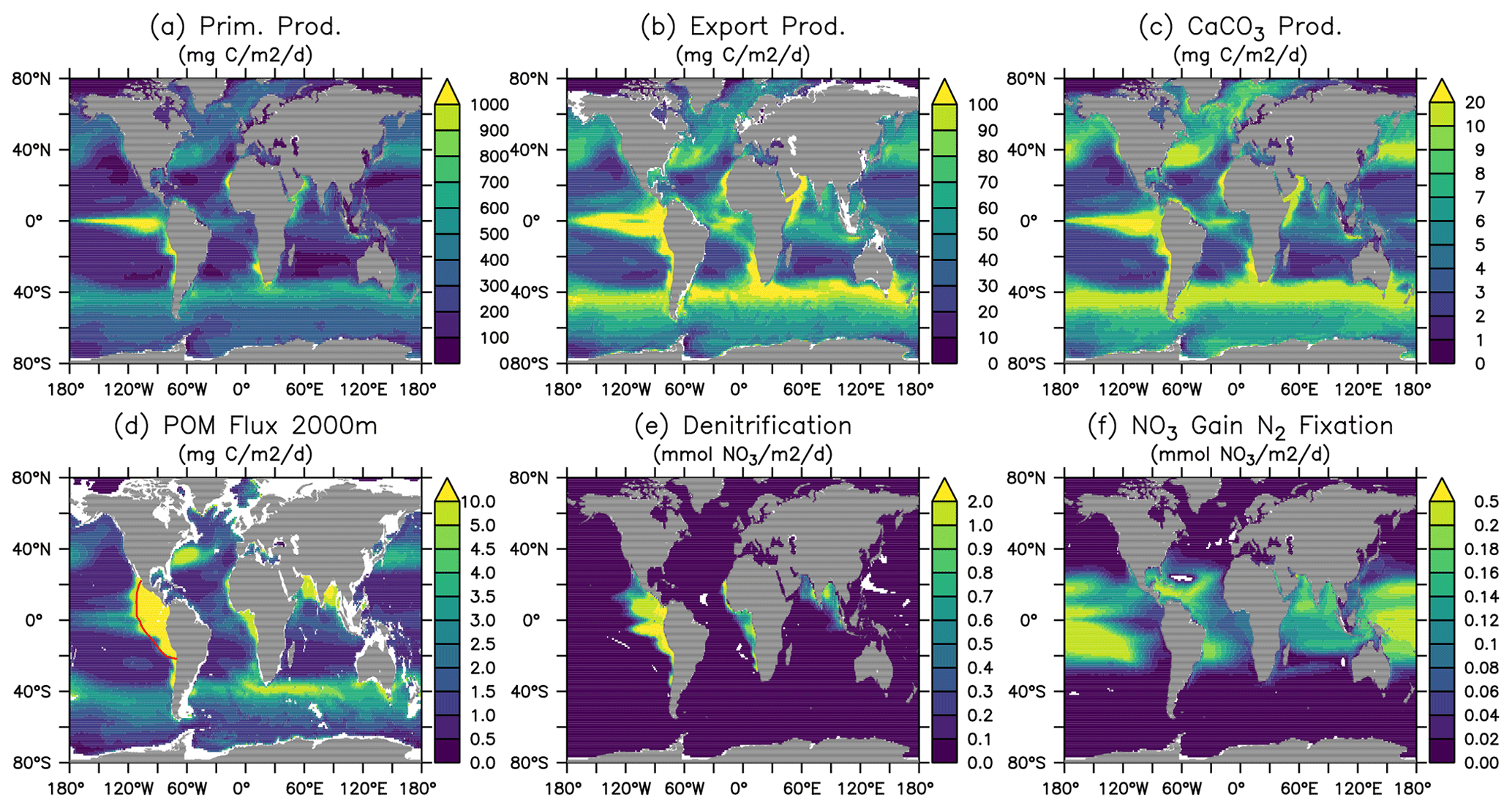
Figure 17Patterns of primary production, export production at 100 m, CaCO3 production, flux of detritus at 2000 m, denitrification, and N2 fixation in the Hist simulations averaged over 2005–2014. The red contour line in (d) indicates an O2 level of 36 mmol O2 m−3. Values are column-integrated except for the export production and the flux of detritus.
3.3.2 Air–sea exchange of carbon
Figure 18 shows the ocean pCO2 and the air–sea CO2 fluxes (positive downwards) in the Hist simulations for the 2005–2014 period, as well as the observation-based estimate for the same period (Landschützer et al. , 2017). In general, sea surface pCO2 and air–sea CO2 flux are affected by various biological and physical processes (Dong et al., 2016; Qu et al., 2022). For example, a too high phytoplankton production could result in a too low DIC and lead to an underestimate of the magnitude of negative CO2 flux (outgassing). Our model results are consistent with such a scenario in the eastern equatorial Pacific, northern Pacific, and parts of the Southern Ocean. The too high phytoplankton production and resultant underestimated DIC could be due to the lack of Fe limitation, as we can see surface PO4 and NO3 are underestimated in the same regions. On the other hand, physical factors such as sea surface temperature (SST; Fig. 19; see Fig. S16 for the standard deviation among the Hist simulations) can also affect pCO2 and CO2 flux. Overestimated SST can be associated with positive pCO2 and negative air–sea CO2 flux biases. Those biological and physical factors result in complex patterns in the pCO2 and CO2 flux, and it is often difficult to quantify the contribution of individual factors. On top of these factors, our model–data comparison is for the period of present-day data (2005–2014). Therefore, the mismatches in pCO2 and CO2 uptake can be from two components: the mismatch inherited from the spin-up at a steady state and the mismatch in the uptake of anthropogenic carbon accumulated during the historical period. Since there are no pre-industrial observations, we cannot differentiate the contributions from each part. Nevertheless, the modelled large-scale pattern of CO2 fluxes and uptake agrees with observations, and the biases in air–sea CO2 fluxes are in the range of other Earth system models participating in the CMIP5 intercomparison (Dong et al., 2016). When zonally averaged, much of the biases are averaged out, and both ocean pCO2 and air–sea CO2 fluxes in FOCI-MOPS match the observations rather well (Fig. 18d and h).
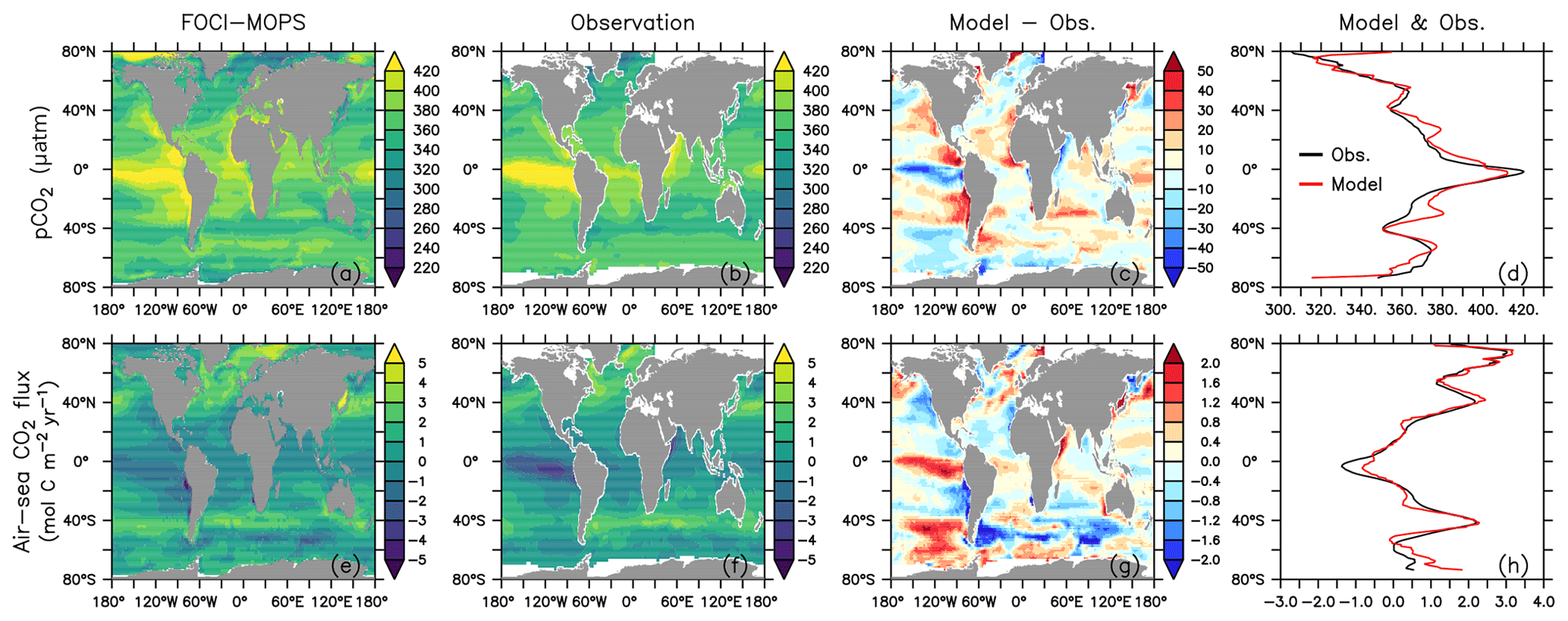
Figure 18Ocean pCO2 and air–sea CO2 fluxes (positive downwards). (a, e) Hist ensemble mean averaged over 2005–2014. Panels (b) and (f) are observations (Landschützer et al. , 2017) over the same time period. Panels (c) and (g) are model biases with respect to the observations, and (d) and (h) are zonally averaged values of observations and model results where observations are available.
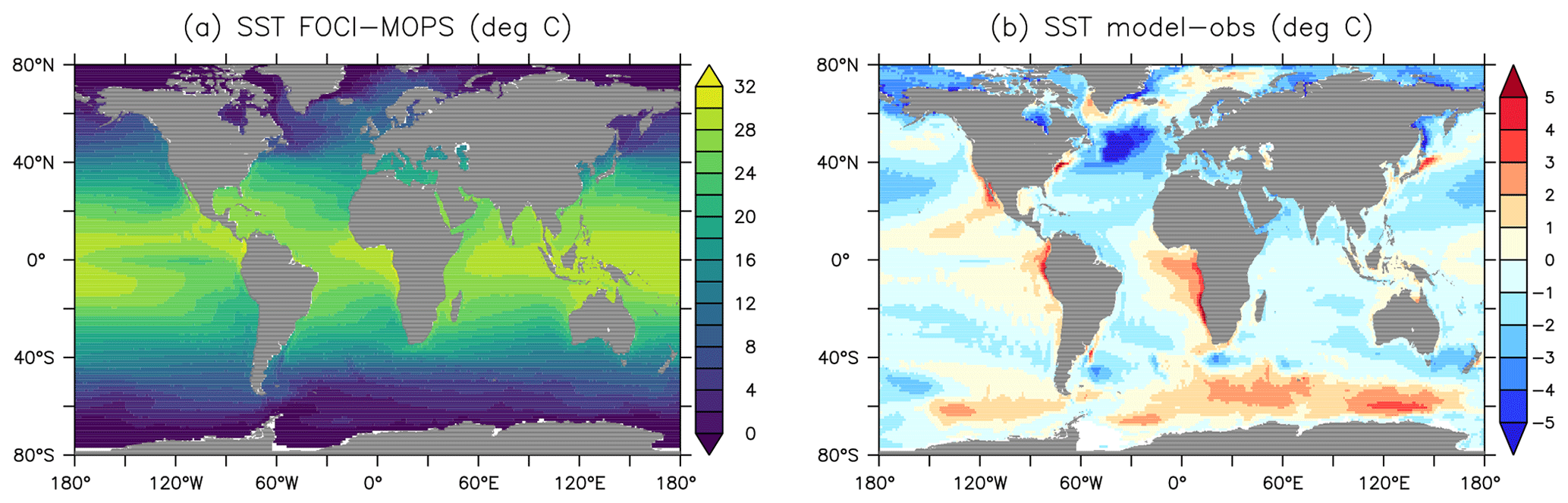
Figure 19Sea surface temperature (SST). (a) Hist ensemble mean averaged over 2005–2014. (b) The difference between model results and observations (HadISST, Rayner et al., 2003).
At high latitudes, the variation in the ocean pCO2 and the air–sea CO2 fluxes are usually higher (Fig. S15) due to the physical mixing being stronger and having higher uncertainty.
3.4 Response to increasing atmospheric CO2
3.4.1 Atmospheric CO2, air–sea CO2 flux, surface air temperature anomaly, and ocean heat content anomaly
Atmospheric CO2 in ESM-piControl drifts slowly from 286.0±0.4 ppm between 1850 and 1879 to 287.1±0.7 ppm between 2005 and 2014, with an average of 286.4±0.14 ppm over the whole period, which is 2 ppm above the prescribed concentration in piControl. During the historical period, atmospheric CO2 in ESM-Hist increases from 286.1±0.46 ppm in 1850 to 410.1±2.33 ppm in 2014, slightly higher than the historical value of 397.5 ppm (Fig. 20a). According to these results, the pre-industrial ocean in FOCI-MOPS acts as a small net CO2 source to the atmosphere. The mean global oceanic CO2 loss in piControl and ESM-piControl during the simulation period are 0.07±0.01 and 0.05±0.01 Pg C yr−1, respectively. In the historical simulations, the globally integrated air–sea CO2 flux gradually increases between 1850 and 1960 along with increasing anthropogenic CO2 perturbation. After 1960, the rate of increase accelerates, and the flux reaches 2.11±0.10 and 2.21±0.14 Pg C yr−1 over 2005–2014 period in Hist and ESM-Hist, respectively, both are slightly lower than the 2.34 Pg C yr−1 estimated by the Global Carbon Project (Friedlingstein et al., 2020; see the summary tab; Fig. 20b).
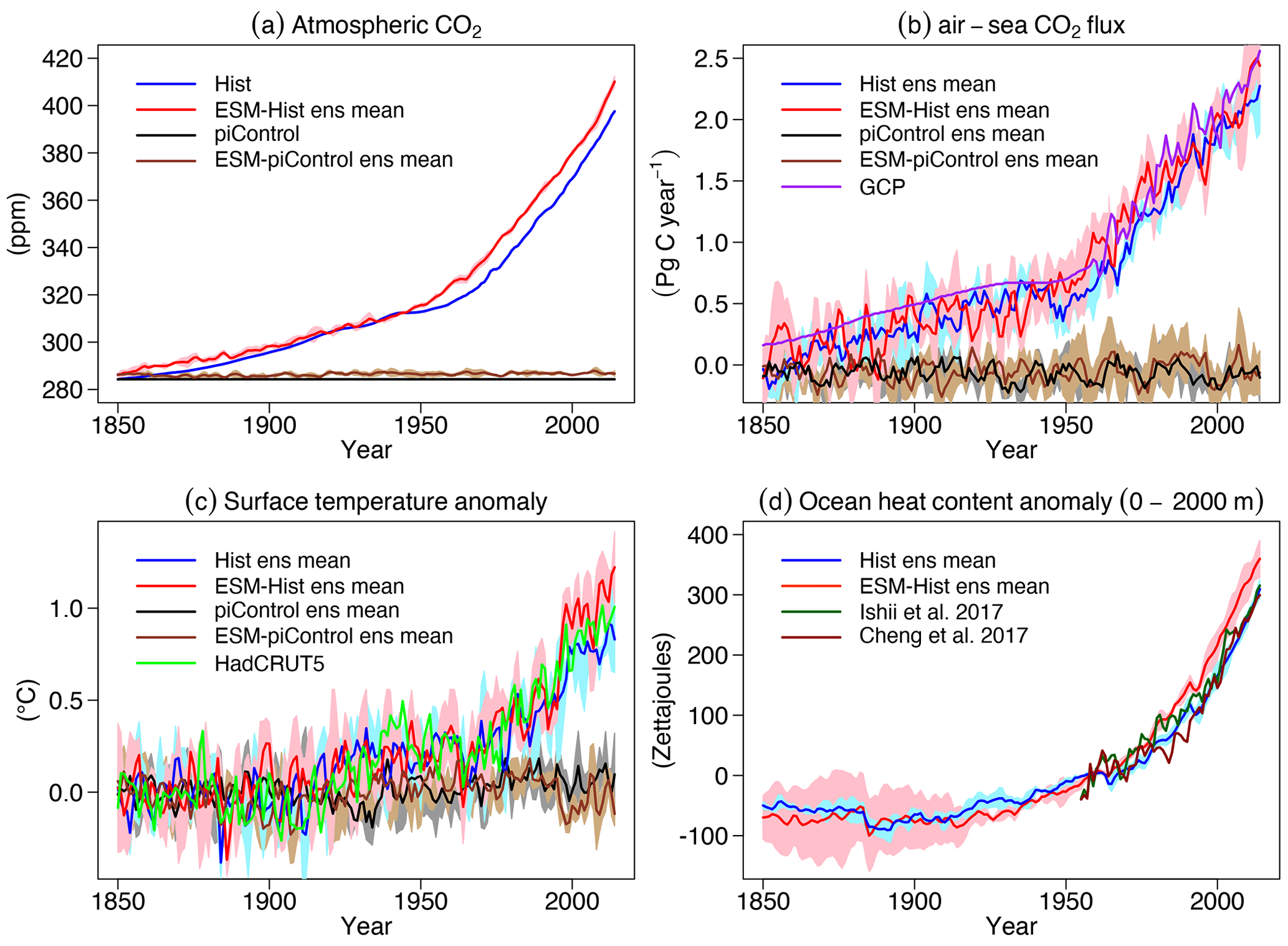
Figure 20Time series of global atmospheric CO2, globally integrated air–sea CO2 fluxes (positive downwards), globally averaged surface temperature, and heat content at 0–2000 m in the ocean of Hist and ESM-Hist. The piControl runs are subtracted to account for drifts. For surface temperature anomalies, the mean values over 1850–1879 are subtracted from the historical period, and for ocean heat content anomalies, the mean values over 1955–1964 are subtracted. (a) Atmospheric CO2 and (b) air–sea CO2 fluxes, (c) surface temperature anomaly, and (d) ocean heat anomaly (0–2000 m) are all given. Grey (blue) and brown (red) lines stand for mean values of concentration-driven and emission-driven pre-industrial control (historical) simulations, respectively. The purple line is air–sea CO2 flux data from the Global Carbon Project (Friedlingstein et al., 2020, see summary tab in the data sheet). The light green line is surface temperature data from HadCRUT5 (Morice et al., 2021). Dark green and brown lines are ocean heat content data from Ishii et al. (2017) and Cheng et al. (2017).
The cumulative air–sea CO2 flux (positive downwards) from 1850 to 2014 in ESM-Hist amounts to 139±2 Pg C, which is 10 Pg C higher than that of Hist, with most of the difference building up over the time period 1850 to 1994 (Table 4). In the land model JSBACH, the air–land carbon flux is fulfilled by the NPP (net primary productivity), which is determined by the difference between photosynthesis and autotrophic respiration of vegetation. The vegetation carbon is lost to grazing by herbivores, litter production, and crop harvests and is consequently transported back to the atmosphere. We have followed Liddicoat et al. (2021) and calculated the compatible emission in the historical simulations. The cumulative compatible emission from 1850 to 2014 in the Hist simulations is 367±3 Pg C, lower than the lower limit of observation (380 Pg C), but agrees with the mean of CMIP6 models when the two highest model values are excluded (367 Pg C, Liddicoat et al., 2021). The underestimated cumulative compatible emission implies missing processes including land carbon uptake during the Second World War, during that period land use might not be correctly accounted for in the model forcing (Bastos et al., 2016). Despite the different cumulative fluxes until 1994, the cumulative CO2 flux is about the same (25±1 Pg C) over 1994 to 2007 in the Hist and ESM-Hist runs (Table 4). Both Hist and ESM-Hist simulate lower cumulative CO2 fluxes when compared with observations and are comparable to or slightly lower than CMIP6 models (Table 4). The cumulative fluxes over 1994–2007 are within the range of observations. The latitudinal distributions of cumulative CO2 fluxes and carbon storage in FOCI-MOPS are consistent with those of CMIP6 models (Fig. 21). The highest CO2 uptake between 40 and 65∘ S is associated with the wind-driven upwelling, which brings deep water with low anthropogenic CO2 to the surface and is able to uptake a higher amount of CO2 (Frölicher et al., 2015). The stronger upwelling seems to be related to the higher variation in CO2 uptake around the similar latitudes within the ensemble and among the CMIP6 models. The anthropogenic CO2 is then transported to the mid-latitudes around 25–40∘ S. A similar pattern occurs in the Northern Hemisphere. The considerable difference between Hist and ESM-Hist simulations around 45–65∘ S is because of the underestimated cumulative compatible emission in the Hist. Nevertheless, the cumulative air–sea CO2 flux is about 10 Pg C higher in the ESM-Hist and is less than 0.03 % of the total DIC inventory, it has an insignificant contribution to the interior DIC distribution between ESM-Hist and Hist (Fig. S17).
(1800–1994; Gruber et al., 2019)(Gruber et al., 2019)(CMIP6 model results; Terhaar et al., 2021)Table 4Cumulative air–sea CO2 fluxes (Pg C) in FOCI-MOPS and observation-based estimates and CIMP6 model results. FOCI-MOPS results are from mean of Hist and ESM-Hist runs. Changes in piControl runs are subtracted from the historical runs.
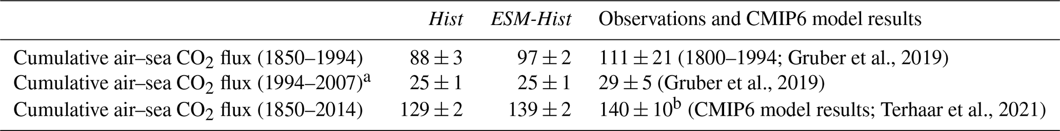
a Including only half of the air–sea CO2 flux in 1994 and in 2007 to be consistent with the data period (mid-1994 to mid-2007)
provided in Gruber et al. (2019).
b Mean of some CMIP6 models, including ACCESS-ESM1-5, CanESM5-CanOE, CanESM5, CESM2, CESM2-WACCM,
CNRM-ESM2-1, GFDL-CM4, GFDL-ESM4, IPSL-CM6A-LR, MPI-ESM1-2-HR, NorESM2-LM, UKESM1-0-LL, and MIROC-ES2L (Terhaar et al., 2021, unconstrained results).

Figure 21Cumulative air–sea CO2 flux (positive downwards) and carbon storage between 1850 and 2014 simulated by FOCI-MOPS and CMIP6 models. The cumulative changes in air–sea CO2 flux over 1850 to 2014 and changes in the carbon storage between 1850 and 2014 in piControl runs are subtracted from the historical runs. Zonally integrated (a) cumulative air–sea CO2 flux and (b) carbon storage. Blue and red lines stand for mean values of Hist and ESM-Hist simulation ensembles of FOCI-MOPS, respectively, and black lines and shaded areas represent the mean and ± standard deviation of some CMIP6 models, including ACCESS-ESM1-5, CanESM5-CanOE, CanESM5, CESM2, CESM2-WACCM, CNRM-ESM2-1, GFDL-CM4, GFDL-ESM4, IPSL-CM6A-LR, MPI-ESM1-2-HR, NorESM2-LM, UKESM1-0-LL, and MIROC-ES2L. Results from MPI-ESM1-2-LR and MRI-ESM2-0 are also included for the carbon storage (Frölicher et al., 2015; Terhaar et al., 2021).
In Hist and ESM-Hist, surface air temperature anomalies remain indistinguishable from piControl and ESM-piControl and only start to increase from the 1920s onwards. The temperature anomalies during 2005–2014 are 0.80±0.05, 1.04±0.12, and 0.93 ∘C in Hist, ESM-Hist, and observations, respectively (Fig. 20c).
The heat content integrated from 0 to 2000 m during 2005–2014 in Hist increased about 257±6 zeta joules (ZJ) from 1955–1964 period, very close to the observations (260–267 ZJ). The increase in ESM-Hist is 317±3 ZJ, 60 ZJ higher than in the Hist, and reflects the higher surface temperature anomalies, which presumably are a consequence of the higher atmospheric CO2 concentrations in experiment ESM-Hist.
In general, Hist and ESM-Hist have a similar temporal evolution and response to anthropogenic forcing, and both largely agree with observations in terms of air–sea CO2 fluxes, temperature, and ocean heat content.
3.4.2 Environmental drivers of marine biogeochemical changes
In addition to the carbon cycle, of particular interest in this study is the impact of climate change on marine biogeochemistry. Several drivers are considered important in this respect, including sea surface temperature (SST), seawater pH, oxygen (O2) and nitrate (NO3) levels, and primary production (PP) (Kwiatkowski et al., 2020). Here we show the temporal evolution of the anomalies of these variables relative to the 1870–1899 reference period, as described in Kwiatkowski et al. (2020). Overall, the anomalies in both Hist and ESM-Hist simulations agree with the range of the CMIP6 mean (Fig. 22). SST anomalies in Hist and ESM-Hist are comparable during the historical period until the year 2000. Between 2005 and 2014, the SST anomaly in ESM-Hist amounts to 0.70±0.13 ∘C, slightly higher than 0.54±0.05 ∘C in Hist (Fig. 22a). In 2014, the 0.23 ∘C higher SST in ESM-Hist compared to Hist is in line with the higher surface air temperature (Fig. 20c). Between 2005 and 2014, the sea surface pH values in Hist and ESM-Hist are 0.095±0.000 and 0.099±0.002 units lower than 1870–1899 (Fig. 22b), respectively. The pH is slightly lower in ESM-Hist than in the Hist simulations due to a higher air–sea CO2 flux (Fig. 20b). The O2 anomalies averaged between 100 and 600 m are mmol O2 m−3 in Hist and mmol O2 m−3 in ESM-Hist simulations between 2005 and 2014 (Fig. 22c), which is equivalent to a decrease of 2 % in both simulations in this depth range. When it comes to the changes in the global O2 inventory, FOCI-MOPS simulated a decrease of 284±32 Tmol O2 per decade over 1960–2010. While the rate is substantially lower than what observations suggest (961±429 Tmol O2 per decade; Schmidtko et al., 2017), such an underestimation of observationally estimated changes in the marine O2 inventory is a common feature among Earth system models (Oschlies et al., 2018). The NO3 concentrations in the euphotic zone (0–100 m) are negatively correlated with SST (Fig. 22d), suggesting a reduced surface supply of NO3 with increasing ocean stratification, a relationship that also exists in other global models (Fu et al., 2016). Similar to the temporal evolution of SST, the NO3 remains relatively unchanged until the 2000s, and the anomalies between 2005 and 2014 are and mmol N m−3 in the Hist and ESM-Hist simulations, respectively (Fig. 22d). Temporal evolutions of PP in Hist and ESM-Hist are similar, and the averaged anomalies over 2005–2014 are % and % in the Hist and ESM-Hist simulations, respectively. These are at the upper end of the PP decrease projected with CMIP6 models (Fig. 22e).

Figure 22Temporal evolution of global mean (a) sea surface temperature (SST), (b) sea surface pH, (c) oxygen (O2) between 100 and 600 m, (d) nitrate (NO3) in the upper 100 m, and (e) vertically integrated primary production (PP) in percentage. Values are relative to the mean of the time period 1870–1899 after subtracting the drifts of the piControl runs. Blue and red lines stand for mean values of Hist and ESM-Hist simulation ensembles of FOCI-MOPS, respectively, and black lines and shaded areas represent the mean and ± standard deviation of CMIP6 models, respectively, as described in Kwiatkowski et al. (2020).
In this study we present the implementation and evaluation of the marine biogeochemistry component coupled to FOCI. The resulting FOCI-MOPS model is based on MOPS (“Model of Oceanic Pelagic Stoichiometry”; Kriest and Oschlies, 2015), which simulates the elemental cycles of oceanic phosphorus, nitrogen, and oxygen between their dissolved (PO4, NO3, O2, and DOM) and particulate (phytoplankton, zooplankton, and detritus) pools. DIC and ALK are included in the implementation, providing a fully coupled carbon cycle in FOCI-MOPS. Spin-up (spinup) and an ensemble of three pre-industrial control (piControl) and historical (Hist) experiments were performed with prescribed atmospheric CO2 concentrations, following the CMIP6 protocols (Eyring et al., 2016). All tracers and fluxes approached steady state or only showed small drifts relative to their mean concentrations in the end of the 500-year spin-up. The marine carbon inventory decreased 0.086 Pg C per year during the last 100 years in the spin-up, which is smaller than the drift suggested as “acceptable” (<0.1 Pg C yr−1) in the Coupled Climate–Carbon Cycle Model Intercomparison Project (C4MIP; Jones et al., 2016). Based on the applied metrics in Table 2, we conclude that FOCI-MOPS reproduces observed biogeochemical patterns of inorganic tracers and phytoplankton/chlorophyll well and that the model's large-scale performance is comparable with other CMIP models. Overall, globally integrated biogeochemical fluxes are in line with observational estimates (Table 3). The spatial patterns of surface ocean pCO2 and air–sea CO2 fluxes agree well with observations (Fig. 18). Simulated changes due to the increasing atmospheric CO2 in globally integrated air–sea CO2 flux and ocean heat content (0–2000 m), as well as globally averaged surface air temperature, also agree well with observations.
We also performed CO2 emission-driven experiments, including ESM-spinup, ESM-piControl, and ESM-Hist. The air–sea CO2 flux in these simulations is slightly higher in the historical emission-driven simulation (ESM-Hist) than in the atmospheric-CO2-driven simulation (Hist), resulting in a higher cumulative air–sea CO2 flux of 139 Pg C relative to 129 Pg C in the Hist between 1850 and 2014. The difference in CO2 perturbation forcing contributes to a higher atmospheric CO2 until the end of the simulation period in ESM-Hist than in the Hist simulations. This higher atmospheric CO2 likely contributes to the higher cumulative air–sea CO2 flux, as well as the higher surface temperatures and ocean heat content in ESM-Hist. Concerning the environmental drivers of marine biogeochemical changes (sea surface temperature, seawater pH, oxygen and nitrate levels, and primary production), their anomalies in both Hist and ESM-Hist simulations agree with the range of the CMIP6 model results (Fig. 22).
We plan to investigate possible shortcomings of the simulated ventilation by direct comparison of simulated and observed abiotic transient tracers (CFCs and SF6). This will better constrain shortcomings in the biogeochemical model component's parameterizations of export and remineralization. We will implement an iron model (Somes et al., 2021) in FOCI-MOPS to improve the potential model deficiency caused by lacking iron limitation in phytoplankton growth. Sensitivity runs with altered remineralization schemes are currently under way. In addition, evaluations of surface seasonal cycle of the model will also be carried out. We plan to use the model to investigate ocean-based CO2 removal approaches for climate change mitigation, such as ocean alkalinity enhancement. While this can be done to some extent with the current model, new parameterizations and improvements in the simulation of ocean carbonate chemistry will likely be required. However, some of this work can only be done when more experimental data is available to constrain the model.
We note that FOCI-MOPS is less complex than most of the biogeochemistry components employed in other Earth system models (Séférian et al., 2020), for instance it does not explicitly resolve silicate or iron cycles and does not consider the CaCO3 saturation state in the dissolution scheme. Nevertheless, as shown by our evaluation in this study, FOCI-MOPS overall shows an adequate performance that makes it an appropriate tool for studying marine biogeochemistry and biogeochemistry–climate interactions in different climate change scenarios, in order to inform the development of emission pathways that are consistent with the agreed climate targets.
The biogeochemical model describes the cycling of phosphorus, nitrogen and oxygen in a stoichiometrically consistent manner (“Model of Oceanic Pelagic Stoichiometry”; Kriest and Oschlies, 2015). The model contains seven components, of which five are calculated in phosphorus units, namely phytoplankton (PHY), zooplankton (ZOO), detritus, dissolved organic matter (DOM), and phosphate (PO4). Additionally, nitrate (NO3) and oxygen (O2) are simulated, with biogeochemical interactions among the different elements coupled via fixed stoichiometric ratios. As the model also simulates NO3 loss and gain through denitrification and nitrogen fixation, respectively, the nitrate-to-phosphate ratio can vary. Details of the model can be found in Kriest and Oschlies (2015), and in Sect. A1 we briefly describe the equations. We have coupled a carbon cycle, which involves the effects of biogeochemical interactions, calcite formation and dissolution on the two additional components of dissolved inorganic carbon (DIC) and alkalinity (ALK), and air–sea gas exchange of CO2 across the sea surface. The implementation of the carbon cycle is described in Sect. A2. Benthic–pelagic exchanges are described in Sect. A3, and a summary of all equations is given in Sect. A4. The biogeochemical model parameters and details on their calibration can be found in Sect. A5.
A1 The biogeochemical model MOPS
A1.1 Plankton dynamics
Phytoplankton (PHY) growth depends on temperature T (f1(T)), daylight intensity (I, (W m−2 d−1)), day length τ (d) (f2(I,τ)), and nutrients (f3(PO4,NO3)). Temperature-dependent growth is formulated following Eppley (1972), in the notation by Schmittner et al. (2008):
where (d−1) is the maximum growth rate of phytoplankton at T=0 ∘C. Light limitation f(I) is parameterized following Smith (1936), integrated over vertical box thickness and day according to Evans and Parslow (1985), in the notation by Evans and Garçon (1997). We note that while the formulation by Evans and Garçon (1997) is based on maximum growth rate and the initial slope of the P–I curve, α ((W m−2)−1 d−1), we here calculate the light limitation based on the half-saturation constant for light, Ic=9.653 (W m−2), as expressed through (thereby resulting in α=0.0622 ((W m−2)−1d−1)):
where I (W m−2 d−1) is the total light during a day at the top of each vertical layer, τ is the length of a day in (fraction of) days, Δz is the vertical box thickness (m), and kw=0.04 (m−1) and kc=0.48 ((mmol P m−3)−1 m−1) are the attenuation coefficients of water and phytoplankton, respectively. The function ϕ is given by (Evans and Garçon, 1997)
The dependence of growth on nutrients f3(PO4,NO3) is based on a Monod function of the least available nutrient X, assuming a constant stoichiometry of phytoplankton given by d=16 (mol N : mol P):
where kPHY=0.031 (mmol P m−3) is the half-saturation constant for phosphate (Kriest et al., 2017). Total phytoplankton growth PP (mmol P m−3 d−1) is then given by the minimum of light and nutrient limitation, but this is only done if the most limiting nutrient is above a certain threshold ( (mmol P m−3)):
Phytoplankton experiences a linear loss given by λPHY=0.03 (d−1). It is grazed by zooplankton (ZOO), where grazing G described by a Holling-III function, with a maximum grazing rate μZOO=1.893 (d−1) and half-saturation constant KZOO=0.086 (mmol P m−3):
Only a fraction ϵZOO=0.75 of grazing G (in (mmol P m−3 d−1)) is effectively ingested, the rest is released again via egestion. Zooplankton further experiences a quadratic mortality κZOO=4.548 ((mmol P m−3)−1 d−1) and a linear excretion rate given by λZOO=0.03 (d−1). Phytoplankton and zooplankton further die with a constant mortality rate of (d−1) but only when present above the lower concentration threshold P (mmol P m−3). Therefore, the source-minus-sink terms due to biogeochemical interactions for phytoplankton () and zooplankton () are
Note that whereas Kriest and Oschlies (2015) assumed that plankton cycling only occurs in the upper, well-lit waters, we here skip this restriction and compute plankton interactions over the full water column. (Of course, production will cease in the aphotic zone because of the light limitation.) Further, we avoid possible negative concentrations because of the Eulerian time-stepping by computing biogeochemical fluxes only when plankton concentrations are positive.
A1.2 DOP and detritus
Dissolved organic matter is implicitly represented by the DOP in phosphorus units in a C : N : P molar ratio of in the model. We assume that a fraction σDOP=0.15 of egestion, quadratic zooplankton mortality, and phytoplankton loss given by λPHY is released as DOP; the rest becomes detritus. Further, phytoplankton and zooplankton mortality leads immediately to the production of DOP. The DOP is remineralized in all layers with a constant rate (yr−1) but only when present above the lower limit of (mmol P m−3). Its oxic and suboxic remineralization further depends on the availability of oxidants oxygen and nitrate, as described by the terms and , which are described in detail in Sect. A1.3 below. Thus, the source-minus-sink term for DOP, , is
Like DOP, detritus (DET) is remineralized with a fixed rate (d−1) to nutrients when present above the lower limit of (mmol P m−3), and its decomposition depends on oxygen and nitrate, as described for the terms and in Sect. A1.3 below. In addition, detritus sinks through the water column. We assume that the sinking speed of detritus increases linearly with depth, according to , where z is the centre of a layer. In steady state and in the absence of any other processes, this parameterization can be regarded as equivalent to the so-called “Martin” (power law) curve of particle flux, with the exponent b given by (see Kriest and Oschlies, 2008, for a detailed discussion). For easier comparison with other model studies, which explicitly define b, and for comparison with empirically observed values for this parameter, in our model experiments we prescribe b=1.41309 and evaluate wlin from it via . Note that in MOPS, due to reduction of remineralization by lack of oxidants (Sect. A1.3), the local effective “Martin” exponent b may be smaller than initially prescribed. The source-minus-sink term of detritus, , is therefore
A1.3 Oxic and suboxic remineralization
If oxygen is above a threshold defined by , with (mmol O2 m−3), organic matter is remineralized aerobically according to a sigmoidal function:
where (mmol O2 m−3) is the half-saturation constant for the heterotroph's uptake of oxygen. To prevent total oxygen consumption per time step from exceeding available oxygen, we first calculate the theoretical oxygen demand for aerobic remineralization of detritus and DOP :
where and are the remineralization rates of DOP and detritus, respectively, and Δt is the time step length of the biogeochemical model. denotes the stoichiometric oxygen demand of aerobic remineralization. The aerobic decay rate limitation is then
Therefore, the sinks of oxygen due to remineralization of DOP and detritus are defined by
If is lower than 36 mmol O2 m−3, denitrification additionally sets in. As for oxygen, we first define a quadratic rate limitation of this process based on a minimum concentration of nitrate, (mmol N m−3), with . To account for inhibition of denitrification by oxygen we further reduce this rate by the inverse oxygen consumption rate:
where (mmol N m−3) is the half-saturation constant for the denitrifiers' uptake of nitrate. As for oxygen, we restrict the use of nitrate to the amount available:
with =0.8 (mmol NO3: mmol P),following the stoichiometry of Paulmier et al. (2009). The rate limitation of anaerobic decay is then
Therefore, the sinks of oxygen and nitrate due to denitrification of DOP and detritus are defined by
A1.4 Nitrogen fixation
As in Kriest and Oschlies (2015), nitrogen fixation depends on temperature and nutrient ratio:
with μNFix=1.88924 (μmol N m−3 d−1) being the maximum nitrogen fixation of the (implicit) cyanobacteria and t2, t1, t0, and tf coefficients that describe the temperature dependency of nitrogen fixation of Trichodesmium spp. (Breitbarth et al., 2007), using the approximation by Kriest and Oschlies (2015). We note that in the model nitrogen fixation only occurs when PO mmol P m−3.
A1.5 Nutrients and oxygen
Phosphate (PO4) is affected by primary production, excretion by zooplankton, and the decay of dissolved and particulate organic matter (POM), as explained above, leading to a source-minus-sink term due to biogeochemical interactions, , of
The loss and gain of nitrate (NO3) follows that of phosphate for aerobic processes and production. In addition, this tracer is affected by denitrification (fixed nitrogen loss) and nitrogen fixation (fixed nitrogen gain):
Finally, oxygen (O2) increases due to photosynthesis and decreases because of aerobic remineralization and respiration by zooplankton.
In addition, oxygen exchanges with the atmosphere at the sea surface (i.e. for layer 1) are given as following Orr et al. (2017).
A2 The carbon cycle
A2.1 Coupling to the biogeochemical core
Photosynthesis decreases DIC, whereas remineralization of organic matter to phosphate increases it. We assume a constant stoichiometry between phosphorus and carbon, a=117 (mol C : mol P); DIC thus changes in proportion to changes in phosphate:
Changes in phosphate and nitrate further affect alkalinity via
A2.2 Calcite production and dissolution
We assume that a constant fraction of detritus production via zooplankton egestion and plankton mortality to detritus is in the form of calcite.
where a=117 (mol C:mol P) is the molar ratio of C : P in organic matter, and (mol CaCO3:mol C) is the calcite-to-organic-carbon ratio. Calcite production reduces DIC by 1 and alkalinity by 2:
Following Schmittner et al. (2008), we integrate the production of calcite over the entire water column:
The total production of calcite is then distributed and dissolved immediately over the entire water column with an e-folding profile , with m, thereby affecting alkalinity and DIC:
and thus the total source-minus-sink terms for DIC and alkalinity due to calcite formation and dissolution are
We note that the redistribution with an e-folding profile over all layers can result in some upward transport of the alkalinity gain caused by calcite dissolution if calcite-bearing detritus produced at greater depths dissolves further up in the water column. It may, however, be just a small problem, as most detritus will likely be produced in shallow layers, where zooplankton grazing and mortality is high.
A2.3 Air–sea gas exchange of CO2 and solution of the carbonate system
The simulation of the carbonate chemistry system and of the air–sea gas exchange of CO2 in MOPS follows an OCMIP-type formulation (Orr et al., 1999) with updates from Orr et al. (2017) for the air–sea gas exchange of CO2.
The air–sea CO2 flux is computed as follows:
where kw (in m s−1) is the gas transfer velocity, (CO)sat (in mol kg−1) is the saturation concentration of CO2, and (CO) (in mol kg−1) is the surface ocean dissolved CO2 concentration (see below for further details). The instantaneous gas transfer velocity kw is parameterized based on Wanninkhof (2014) as a quadratic function of the 10 m wind speed u:
where ξ is a constant, Sc is the Schmidt number, and fice is the fraction of the grid cell covered by sea ice.
The saturation concentration of CO2 in equilibrium with the water-vapour-saturated atmosphere at a total atmospheric pressure of 1 atm (i.e. (CO)sat) is computed as follows:
where xCO2 is the mole fraction of CO2 in dry air and F is the solubility function (Weiss and Price, 1980, Eq. (13), Table 6, column 3), which includes all non-ideal effects and fits the effects of water vapour pressure for a total atmospheric pressure of 1 atm.
Once dissolved, CO2 reacts with seawater, forming carbonic acid (H2CO3), most of which dissociates into two other inorganic species, bicarbonate (HCO) and carbonate (CO) ions. CO refers to the sum of dissolved CO2 and the much less abundant H2CO3. The sum of the three species CO + HCO + CO is referred to as total dissolved inorganic carbon (DIC). Their partitioning depends on seawater pH, temperature, salinity, and pressure. The pH may be calculated from DIC and seawater's ionic charge balance, formalized as total alkalinity (ALK). DIC and ALK are carried as prognostic tracers in the ocean model, and both are used, along with temperature, salinity, and nutrient concentrations, to compute CO at the ocean surface.
The carbonate chemistry system is solved using the equilibrium constants recommended for best practices (Dickson et al., 2007). The total pH scale is used for all constants except Ks (which uses the “free” scale following Dickson, 1990). The model does not explicitly simulate boron, sulfate, and fluoride, which are instead estimated as function of chlorinity based on Lee et al. (2010) (for boron), Morris and Riley (1966) (for sulfate), and Riley (1965) (for fluoride). Silicate, which is also not explicitly simulated, is computed as a function of density following Orr et al. (1999).
For reasons of computational efficiency, to solve the carbonate chemistry system we use the approximate and non-iterative method proposed by Follows et al. (2006) (Eqs. 8, 11, and 12 therein). The algorithm has been shown to provide a sufficiently accurate solution in the context of a three-dimensional global ocean carbon cycle model. The algorithm uses DIC, ALK, dissolved inorganic phosphorus, silica, boron, and thermodynamic equilibrium coefficients as inputs. The species retained in the expression for alkalinity are the phosphoric, silicic, carbonic, boric, sulfuric, fluoridic, and water acid systems. Starting from an initial guess of pH deriving from the previous time step, the formula provides an updated value of pH as output, which is then used to compute CO (Eq. 8 in Follows et al., 2006) and surface CO2 fugacity as follows:
where K0 is the solubility coefficient of CO2 in seawater (Eq. 12 and column 3 of Table 1 in Weiss, 1974).
A3 Benthic burial and nutrient re-supply
As in Kriest and Oschlies (2013) and Kriest and Oschlies (2015), we assume that once sinking detritus arrives at the seafloor a fraction of it is buried in the sediments. The amount buried, (mmol P m−2 d−1), depends on the rain rate of detritus to the sea floor (FB, (mmol P m−2 d−1)) via
where k is the index of each vertical box (counting downwards) and kb is the last ocean box above the sea floor at each horizontal model grid point.
In contrast to Kriest and Oschlies (2013) and Kriest and Oschlies (2015), the amount buried is not integrated globally and over a year and then resupplied to the ocean via river runoff; instead, in every time step the global amount of organic phosphorus, nitrogen, and buried content is resupplied at the sea surface (in the surface layer) as phosphate, nitrate, and DIC. Thus, if is the global burial in a time step integrated over the sea floor area A and V1 is the global volume of the surface layer,
We note that this approach has a slightly “fertilizing” effect even away from the river mouths. To account for the implicit, simultaneous burial of particulate organic carbon and nitrogen, the respective supply of nitrate and DIC is parameterized using constant stoichiometry:
We also account for the equivalent of negative alkalinity (that would be consumed when organic matter was remineralized instead of being buried) by subtracting it from alkalinity at the sea surface:
In contrast to organic material, we assume no burial of calcite in the sediment but dissolve all calcite arriving in the bottom box immediately.
A4 Total source-minus-sinks
Summing up the effects of all processes, we arrive at the following equations for the source-minus-sink terms:
A5 Parameter calibration
The biogeochemical model parameterization is based upon a previous objective calibration of model MOPS coupled to the Transport Matrix Method (Khatiwala, 2007; Khatiwala et al., 2018), using Transport Matrices derived from the ECCO project (Kriest et al., 2020). In particular, Kriest et al. (2020) optimized the parameters for oxidant-dependent remineralization NO, , , the maximum nitrogen fixation rate μNFix, the oxygen requirement for aerobic remineralization, and the parameter determining the particle flux profile b against observed nutrients and oxygen at a global scale, while all other parameters were kept constant.
However, when comparing parameters optimized for different circulations, Kriest et al. (2020) noted that three of the six parameters optimized were sensitive to characteristic features of the applied circulation, as expressed through the maximum mixed layer depth, age of North Atlantic Deep Water (NADW), and outcrop area of Sub-Antarctic Mode Water (SAMW) and Antarctic Intermediate Water (AAIW). We therefore adjusted , b, and μNFix to the values for the respective physical diagnostic of NEMO by using the regression shown in Fig. 6 of Kriest et al. (2020). The adjustment led to a higher value for (165.08044 instead of 151.1 mol O2: mol P), a slightly lower value for b (1.41309 instead of 1.46), and a lower value of μNFix (1.88924 instead of 2.29 μmol N m−3 d−1; see also Table A1).
Table A1Biogeochemical model parameters of MOPS (see also Kriest et al., 2020) and for the carbon cycle.
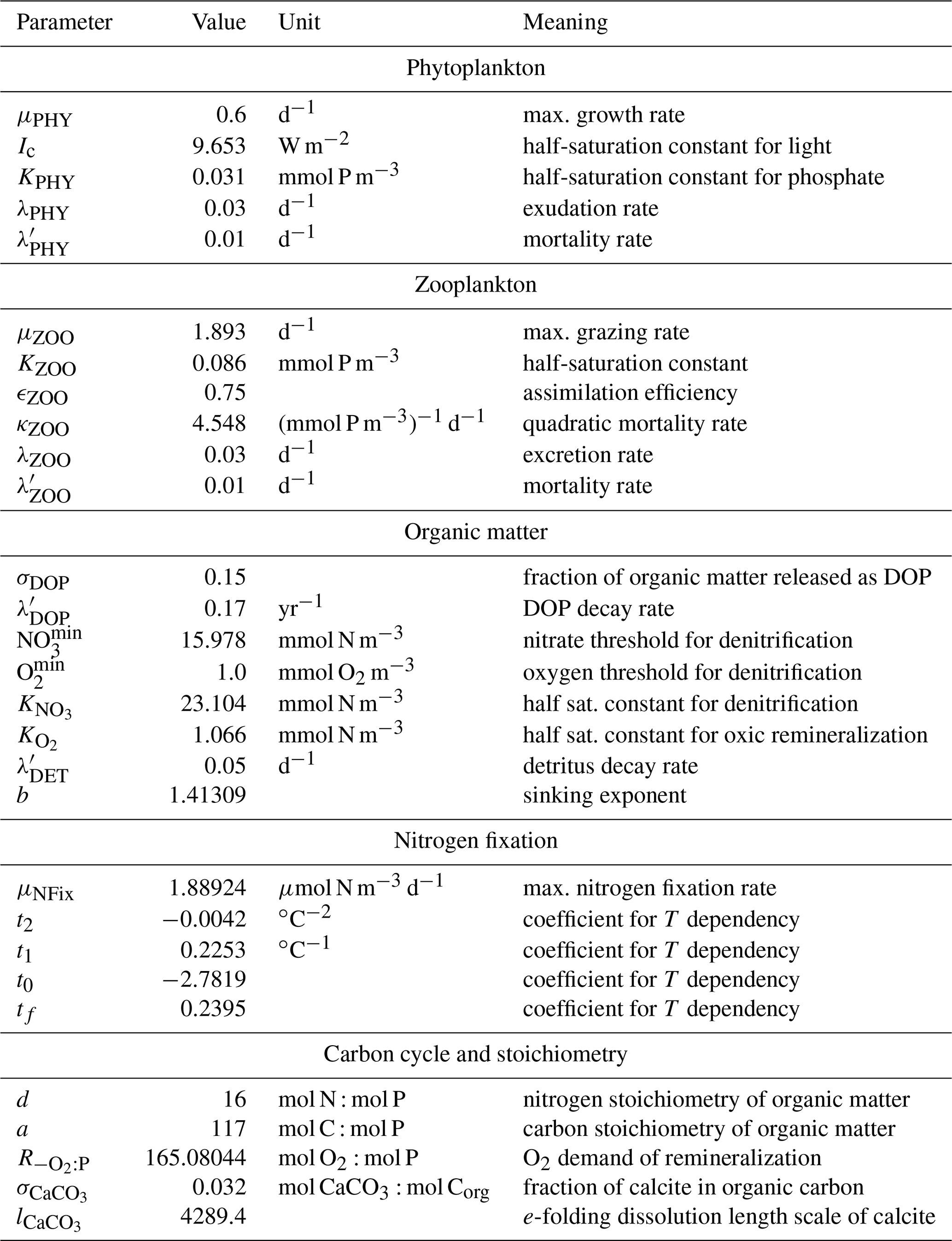
To adjust the parameters regarding the calcite cycle, we have extended MOPS in the setup ECCO described by Kriest et al. (2020) to include the carbon cycle described above but with a slightly different air–sea gas exchange and computation of the carbonate system, and we have optimized and after a spin-up of 10 years against a data set of alkalinity and preindustrial DIC. The resulting parameters are only slightly different from those applied by Schmittner et al. (2008), namely mol CaCO3: mol Corg (instead of 0.035 mol CaCO3: mol Corg) and m (instead of 3500 m).
B1 Model postprocessing
The model geometry is based on a curvilinear grid, complicating a direct comparison to observations, which are mostly available on regular (rectangular) grids. Thus, we have mapped the model output onto a horizontal grid defined by using Ferret's functions curv_to_rect_map (with a radius of 2∘ for map creation) and curv_to_rect. The vertical grid of NEMO was maintained. All further analysis of model fit was carried out on these remapped quantities unless stated otherwise.
B2 Data sets for model validation
For a complete biogeochemical model evaluation we used data sets of phosphate, nitrate, oxygen, DIC, total alkalinity, surface chlorophyll, mesozooplankton, and particulate and dissolved organic matter. Because many of the observed quantities are available in different spatial resolutions, they were gridded onto the rectangular model grid. Further details, including conversion from different units, are described below.
B2.1 Nutrients, oxygen, DIC, and alkalinity
For the spatial distribution (Sect. 3.2.1) comparisons of dissolved inorganic tracers we used the interpolated data, and for model evaluation with statistical metrics (Sect. 3.2.3) we used the non-interpolated data of the Global Ocean Data Analysis Project version 2 mapped climatology (GLODAPv2.2016b, Lauvset et al., 2016; Olsen et al., 2016), as available at https://www.nodc.noaa.gov/ocads/oceans/GLODAPv2_2020/ (last access: 12 May 2016). Observed concentrations of all inorganic tracers have been converted from μmol kg−1 to mmol m−3 using in situ density computed from GLODAP's temperature and salinity. Originally the non-interpolated data set contained between 158 401 and 252 808 data points for the different tracers because the NEMO grid, onto which the data are interpolated, has a higher vertical resolution; the final data set contains between 183 213 and 295 603 data points (see Table B1).
Lauvset et al. (2016)Olsen et al. (2016)Melin (2013)Moriarty and O'Brien (2013)Martiny et al. (2014)Torres-Valdés et al. (2009)Moutin et al. (2008)Yoshimura et al. (2007)Table B1Statistics for observations, regridded onto model grid: number of observations, minimum and maximum concentration, volume-weighted mean, and standard deviation. See Sect. B2 for further details.
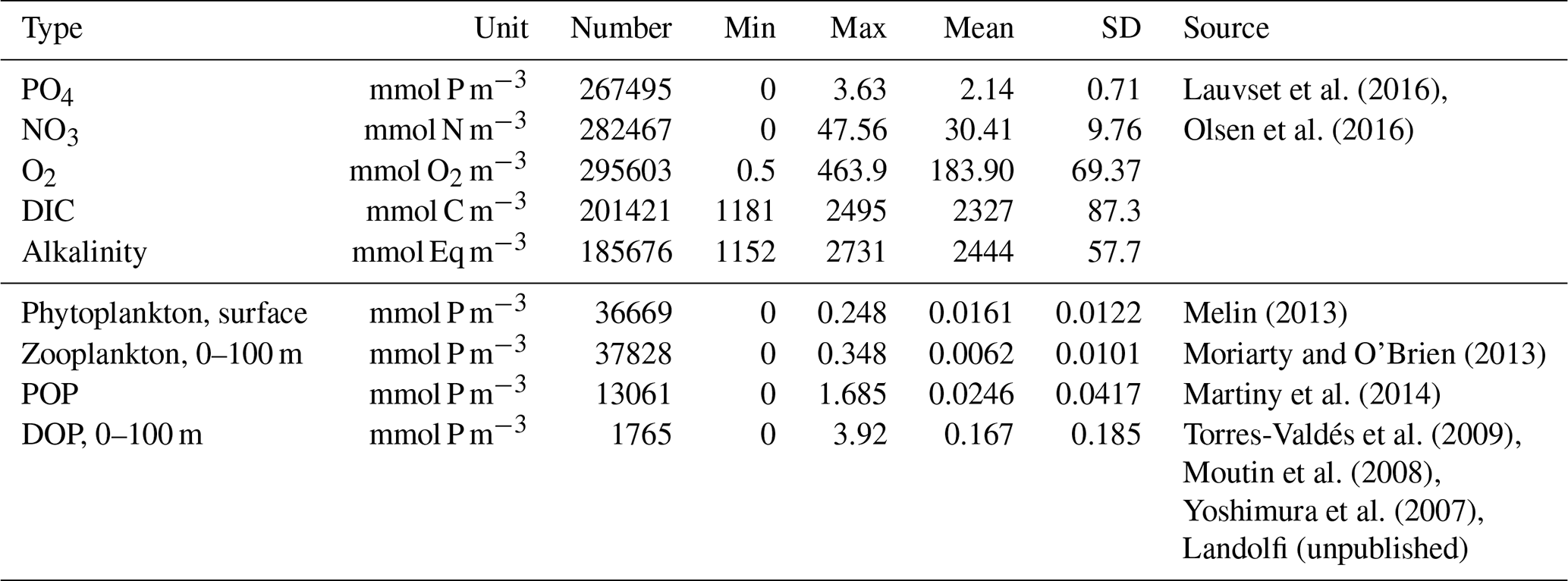
B2.2 Phytoplankton
For the assessment of simulated phytoplankton we use chlorophyll data derived from remote sensing (MODIS-Aqua; Melin, 2013, https://jeodpp.jrc.ec.europa.eu/ftp/public/JRC-OpenData/GMIS/satellite/9km/climatology/, last access: 20 January 2021). The original surface data are available as a monthly climatology on a 9 km grid. After averaging to annual mean chlorophyll, the data are gridded (by averaging) onto a horizontal grid defined by . Chlorophyll was converted to carbon using the algorithm derived by Sathyendranath et al. (2009) and then to phosphorus using a C : P ratio of 117 mol C : mol P. The resulting data set contains 36.669 data points, which are all located in the surface layer, with minimum and maximum values of 0 and 0.25 mmol P m−3, respectively, an unweighted mean of 0.0161 mmol P m−3, and a standard deviation of 0.0122 mmol P m−3 (see Table B1).
B2.3 Zooplankton
For the evaluation of simulated zooplankton we use the MAREDAT data set of mesozooplankton (Moriarty and O'Brien, 2013). This sparse, quasi-climatological data set contains 42.245 data points of monthly mean mesozooplankton (in mg C m−3) on a degree grid. After averaging over a year, and mapping onto the spatial grid of NEMO, we obtained a total of 37.838 data points for the upper 100 m. Conversion to phosphorus was carried out by assuming a C : P ratio of 117 mol C : mol P.
Many groups of mesozooplankton carry out diurnal vertical migration, meaning that they descend to depths between ≈200–500 m depth at dawn and ascend to the surface layers for feeding at dusk (e.g., Kiko et al., 2017, 2020). This process is so far not included in the model (see Aumont et al., 2017), and may lead to an overestimation of simulated zooplankton biomass when compared only against surface data. Therefore, to account for the maximum total potential biomass of grazers in the observations, we integrated all observed biomass within the upper 500 m and distributed it evenly over the upper 100 m for model comparison.
Further, the biogeochemical model does not distinguish between microzooplankton and mesozooplankton but aggregates both types into one single component. Unfortunately, samples for microzooplankton are much more sparse (only 2029 monthly data in the data set by Buitenhuis et al., 2012) than those of mesozooplankton and are often taken at other locations and during other times. Based on an analysis at stations where both small and large zooplankton observations are available, we estimated an approximate micro-to-mesozooplankton ratio of 1. For comparison with the model we therefore doubled the observed concentrations of mesozooplankton, resulting in minimum and maximum concentrations of 0 and 0.348 mmol P m−3, an average of 0.0062 mmol P m−3, and a standard deviation of 0.0101 mmol P m−3 (see Table B1).
B2.4 POP
There is no direct observational equivalent to simulated detritus; the closest type of observation are those of particulate organic phosphorus (POP), nitrogen (PON), or carbon (POC). For model evaluation we downloaded the data set by Martiny et al. (2014, https://datadryad.org/stash/downloads/file_stream/87679, last access: 16 April 2020), which contains observations of POP, PON, and POC. After omitting some entries where depth was not given, we obtained 6940 data points for POP and 46 705 data points for PON. Because of the much higher data frequency for PON, we used this variable as further diagnostic, and converted it to POP using a stoichiometric ratio of 16 mol N : mol P.
To map data onto a regular grid we averaged all data that fall within boxes defined by a horizontal resolution of and 23 depth intervals centred at 5, 15, 27.5, 45, 65, 87.5, 117.5, 160, 222.5, 310, 435, 610, 847.5, 1160, 1542.5, 1975, 2450, 2950, 3450, 3950, 4450, 4950 and 5450 m. The resulting data set contained 6887 data points for PON, with minimum and maximum concentrations (after conversion to POP) of 0 and 1.69 mmol P m−3, respectively, an average of 0.0266 mmol P m−3, and a standard deviation of 0.0499 mmol P m−3. Following this mapping, we interpolated the data onto the NEMO grid. Because of the higher vertical resolution of NEMO, this data set contains more observations but similar statistics (see Table B1).
Particulate organic matter is usually collected with Niskin bottles and then filtered; thus it entails not only detritus (dead organic particles) but also phytoplankton and possibly a fraction of zooplankton. We therefore compare these observations to the sum of simulated detritus and phytoplankton plus half of the zooplankton, thereby assuming that microzooplankton is caught in the Niskin bottles and remains on filters for PON analysis.
B2.5 DOP
Most observations of dissolved organic phosphorus applied for model evaluation have been compiled by Angela Landolfi. They include data from cruises 36N, AMT10, AMT12, AMT14, AMT15, AMT16, and AMT17 (Torres-Valdés et al., 2009); the BIOSOPE cruise (Moutin et al., 2008); a cruise of the North Atlantic (cruise D279, April–May 2004; Landolfi et al., 2016); and the unpublished data from the Indian Ocean (cruise CD139, March–April 2002; Landolfi, unpublished). The coefficient of variation of DOP measurements is about 10 % in Landolfi et al. (2016). In the compilation we only included data with a positive (good) quality flag. We further included data from the northern Pacific from Fig. 2 of Yoshimura et al. (2007). Data were gridded onto a grid with 23 vertical layers, as applied for mapping of PON. After mapping onto this grid we obtained 814 data points in the upper 100 m, with minimum and maximum values of 0 and 3.92 mmol P m−3, an average of 0.178 mmol P m−3, and a standard deviation of 0.21 mmol P m−3. Gridding onto the finer NEMO grid increases the number of observations but largely maintains the statistics (see Table B1). Note that the majority of the surface observational data (phytoplankton, zooplankton, POP, and DOP) were collected between spring and autumn, and potential biases could exist when compared with annual mean model results.
B3 Metrics
To assess the performance of the biogeochemical model we apply six statistical measures and metrics that account in different ways for potential errors in average concentrations (biases), the spatial variability of observations, and the match to spatial patterns. In particular we evaluated the model bias (both absolute and normalized by the observed mean), the model's standard deviation σM normalized by the standard deviation of observations σO, the root-mean-squared error (RMSE), the pattern error or centred rms difference RMSE′ (RMSE minus bias), and the correlation coefficient r between model and observations. All calculations take into account the spatial dimensions of the model, thereby emphasizing deviations in the deep ocean, where box thicknesses are large. To investigate the model's representation of dissolved inorganic tracers in different vertical domains, beside the global model fit we also evaluated the metrics in different vertical domains, namely for 0–100, 100–200, 200–500, 500–1000, 1000–2000, and 2000–5000 m. Vertical domains of the organic tracers are surface for phytoplankton, the upper 100 m for zooplankton and DOP (see above for treatment of zooplankton observations), and the full domain for POP.
A slight distortion in the physical model (e.g. a current being located slightly off) may cause a large RMSE and thereby induce a large model error, even if the biogeochemical model is dynamically correct. To account for this, and to compare this model with the results by Ilyina et al. (2013), we further added a seventh metric, namely the Bhattacharyya distance (BD), which evaluates the similarity between observed and simulated frequency distributions of tracers. In particular, to evaluate BD we binned simulated and observed tracer concentrations into N=50 concentration classes over a typical range of concentrations (phosphate: 0–4 mmol P m−3; nitrate: 0–50 mmol N m−3; oxygen: 0–400 mmol O2 m−3; DIC and alkalinity: 1700–2500 mmol m−3; phytoplankton and zooplankton: 0–0.1 mmol P m−3; POP: 0–0.5 mmol P m−3; DOP: 0–1 mmol P m−3). Examples for different distributions are given in Figs. B1 and 16. Following binning, BD was evaluated as
where mi and oi are the frequencies of simulated and observed model boxes with concentration of class i. We note that BD relates to the Hellinger distance (HD) via BD as follows:
In contrast to the BD, the HD is bounded by . Finally, the L1 norm of distributions as given by the following equation is evaluated (note that this norm is bounded by ).
Figures B1 and 16 list the different metrics of inorganic and organic tracers in different vertical domains. In all cases, the smaller the area of overlap between the two distributions, the larger the metric will be.
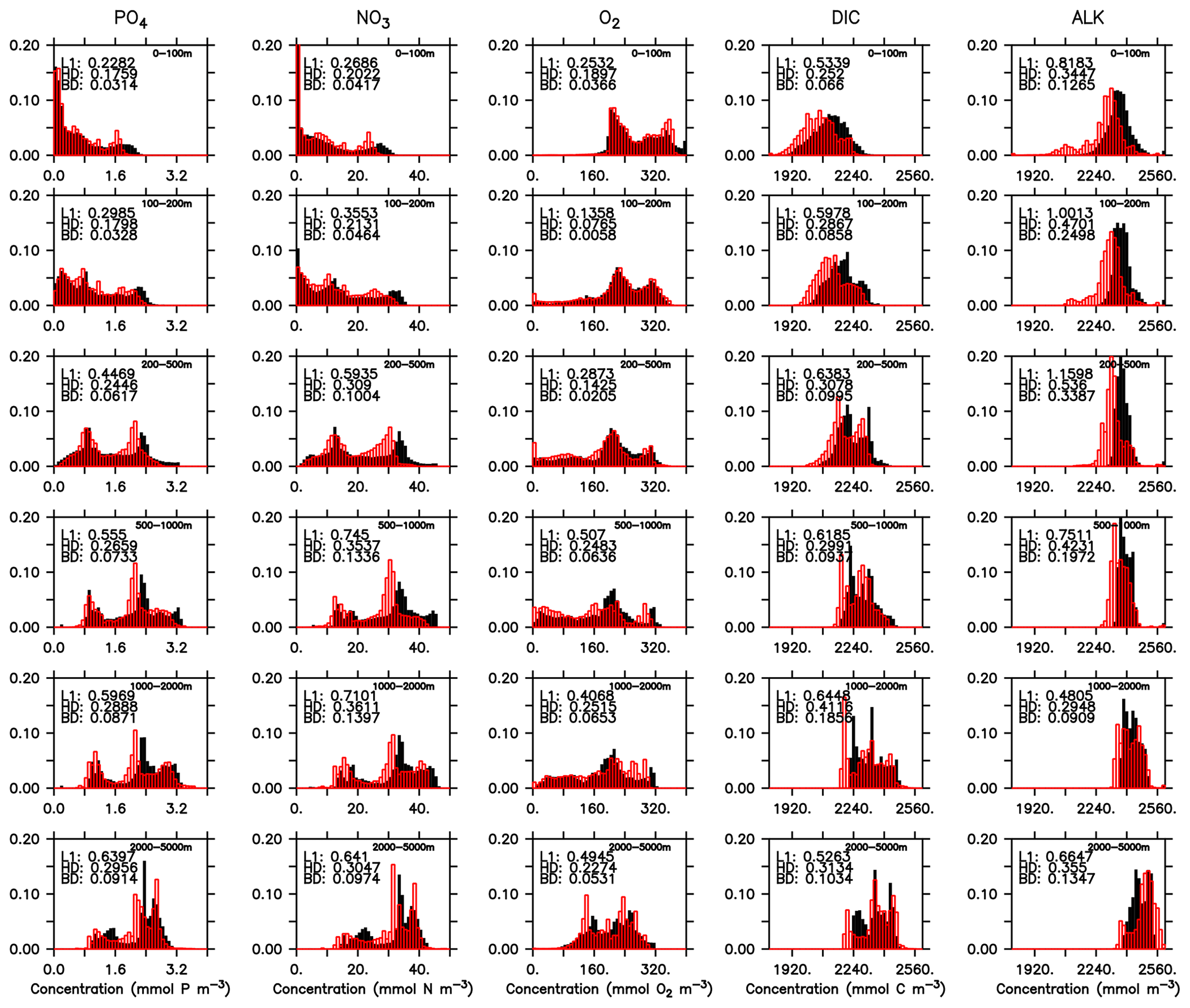
Figure B1Frequency distribution of phosphate, nitrate, oxygen, DIC, and alkalinity (left to right) from observations (black filled bars) and the model (red bars) for different vertical domains (top to bottom). Numbers denote three different metrics for the similarity of the distributions, namely L1 (Eq. B3), HD (Eq. B2), and BD (Eq. B1).
Table B2Different metrics for surface (0–100 m), total domain (0–8000 m) and range of metrics over seven different vertical domains (0–100, 100–200, 200–500, 500–1000, 1000–2000, 2000–5000, 0–8000 m) of historical experiments ensemble mean from 1972 to 2013 for PO4, NO3, O2, ALK; 2002 for DIC; and 2005–2014 for Phy, Zoo, POP, and DOP. Different metrics include the correlation coefficient (r), the root-mean-squared error (RMSE), the pattern error (RMSE′, RMSE minus global bias), the global bias (in mmol m−3), bias normalized by observed global mean, normalized standard deviation, and the Bhattacharyya distance (BD) for each model component. Except for BD, all metrics have been calculated on a volume-weighted basis. See the text for further details.
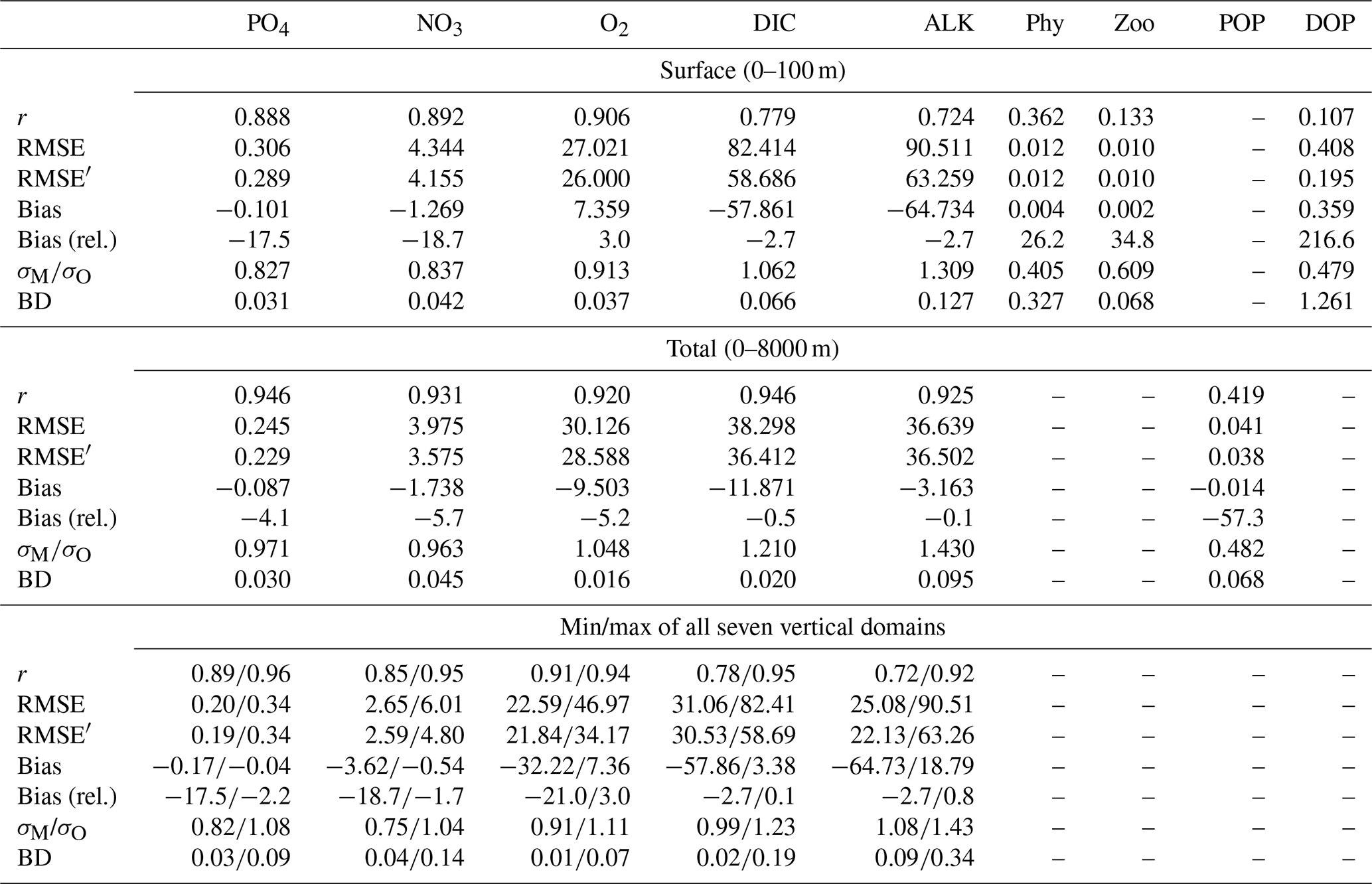
The FOCI-MOPS is build based on a published FOCI version (Matthes et al., 2020). All modifications to the published version code and full runtime environment are provided at https://doi.org/10.5281/zenodo.6772175 (Chien et al., 2022). Model data and codes necessary to reproduce the figures present here are available at the same location. All data used in this paper are publicly accessible, including World Ocean Atlas 2013 (https://www.ncei.noaa.gov/products/ocean-climate-laboratory, last access: 15 August 2020, Garcia et al., 2013a, b), Global Ocean Data Analysis Project version 2 mapped climatology (GLODAPv2.2016b, https://www.glodap.info/index.php/mapped-data-product/, last access: 12 May 2016, Lauvset et al., 2016; Olsen et al., 2016), surface pCO2 and air–sea CO2 fluxes (https://www.ncei.noaa.gov/access/ocean-carbon-acidification-data-system/oceans/SPCO2_1982_2015_ETH_SOM_FFN.html, last access: 21 July 2022, Landschützer et al. , 2017), chlorophyll (https://jeodpp.jrc.ec.europa.eu/ftp/public/JRC-OpenData/GMIS/satellite/9km/climatology/, last access: 20 January 2021, Melin, 2013), microzooplankton (https://doi.org/10.1594/PANGAEA.779970, Buitenhuis et al., 2012), mesozooplankton (https://doi.org/10.1594/PANGAEA.785501, O'Brien and Moriarty, 2012; Moriarty and O'Brien, 2013), AMOC (RAPID, https://rapid.ac.uk/rapidmoc/rapid_data/datadl.php, last access: 21 July 2022, McCarthy et al., 2015), POM (https://datadryad.org/stash/downloads/file_stream/87679, last access: 21 July 2022, Martiny et al., 2014), SST (HadISST, https://www.metoffice.gov.uk/hadobs/hadisst/data/download.html, last access: 21 July 2022, Rayner et al., 2003), SST anomaly (HadCRUT5, https://www.metoffice.gov.uk/hadobs/hadisst/data/download.html, last access: 21 July 2022, Morice et al., 2021), and air–sea CO2 flux (Global Carbon Project, https://www.icos-cp.eu/science-and-impact/global-carbon-budget/2020, Global Carbon Project, 2020; Friedlingstein et al., 2020).
The supplement related to this article is available online at: https://doi.org/10.5194/gmd-15-5987-2022-supplement.
DE, IK, JVD, and LP implemented the MOPS codes into the FOCI. CTC and JVD carried out simulations with assistance of SW. JVD designed the experiment with assistance from DPK, WK, IF, AO, and IK. AL compiled the DOP data. All authors discussed the results and wrote the manuscript.
The contact author has declared that none of the authors has any competing interests.
Publisher's note: Copernicus Publications remains neutral with regard to jurisdictional claims in published maps and institutional affiliations.
Parallel supercomputing resources have been provided by the North German Supercomputing Alliance (HLRN). The authors wish to acknowledge use of the Ferret program of NOAA's Pacific Marine Environmental Laboratory for analysis and graphics featured in this paper.
Dana Ehlert and Jonathan V. Durgadoo were supported by the Helmholtz-Gemeinschaft for the research project “Advanced Earth System Modelling Capacity” (grant no. ZT-0003). Chia-Te Chien was supported by the OceanNETs project, which has received funding from the European Union's Horizon 2020 research and innovation programme under grant no. 869357, and the Deutsche Forschungsgemeinschaft (DFG; project no: CH 2605/1-1). Lavinia Patara was financially supported by the GEOMAR Helmholtz Centre for Ocean Research Kiel and by the project CP1219 of the Cluster of Excellence “The Future Ocean” funded by the DFG.
The article processing charges for this open-access publication were covered by the GEOMAR Helmholtz Centre for Ocean Research Kiel.
This paper was edited by Paul Halloran and reviewed by Jerry Tjiputra and Timothée Bourgeois.
Anderson, L. A. and Sarmiento, J. L.: Redfield ratios of remineralization determined by nutrient data analysis, Global Biogeochem. Cy., 8, 65–80, https://doi.org/10.1029/93GB03318, 1994. a
Arneth, A., Harrison, S. P., Zaehle, S., Tsigaridis, K., Menon, S., Bartlein, P. J., Feichter, J., Korhola, A., Kulmala, M., O'Donnell, D., Schurgers, G., Sorvari, S., and Vesala, T.: Terrestrial biogeochemical feedbacks in the climate system, Nat. Geosci., 3, 525–532, https://doi.org/10.1038/ngeo905, 2010. a
Aumont, O., van Hulten, M., Roy-Barman, M., Dutay, J.-C., Éthé, C., and Gehlen, M.: Variable reactivity of particulate organic matter in a global ocean biogeochemical model, Biogeosciences, 14, 2321–2341, https://doi.org/10.5194/bg-14-2321-2017, 2017. a
Balch, W., Drapeau, D., Bowler, B., and Booth, E.: Prediction of pelagic calcification rates using satellite measurements, Deep Sea Research Part II: Topical Studies in Oceanography, 54, 478–495, https://doi.org/10.1016/j.dsr2.2006.12.006, 2007. a
Bastos, A., Ciais, P., Barichivich, J., Bopp, L., Brovkin, V., Gasser, T., Peng, S., Pongratz, J., Viovy, N., and Trudinger, C. M.: Re-evaluating the 1940s CO2 plateau, Biogeosciences, 13, 4877–4897, https://doi.org/10.5194/bg-13-4877-2016, 2016. a
Berthet, S., Séférian, R., Bricaud, C., Chevallier, M., Voldoire, A., and Ethé, C.: Evaluation of an Online Grid-Coarsening Algorithm in a Global Eddy-Admitting Ocean Biogeochemical Model, J. Adv. Model. Earth Sy., 11, 1759–1783, https://doi.org/10.1029/2019MS001644, 2019. a
Bhattacharyya, A.: On a Measure of Divergence between Two Multinomial Populations, Sankhya, 7, 401–406, 1946. a
Bianchi, D., Dunne, J. P., Sarmiento, J. L., and Galbraith, E. D.: Data-based estimates of suboxia, denitrification, and N2O production in the ocean and their sensitivities to dissolved O2, Global Biogeochem. Cy., 26, GB2009, https://doi.org/10.1029/2011GB004209, 2012. a
Breitbarth, E., Oschlies, A., and LaRoche, J.: Physiological constraints on the global distribution of Trichodesmium – effect of temperature on diazotrophy, Biogeosciences, 4, 53–61, https://doi.org/10.5194/bg-4-53-2007, 2007. a
Brovkin, V., Raddatz, T., Reick, C. H., Claussen, M., and Gayler, V.: Global biogeophysical interactions between forest and climate, Geophys. Res. Lett., 36, L07405, https://doi.org/10.1029/2009GL037543, 2009. a
Buitenhuis, E. T., Rivkin, R. B., Sailley, S., and Le Quéré, C.: Global distributions of microzooplankton abundance and biomass – Gridded data product (NetCDF) - Contribution to the MAREDAT World Ocean Atlas of Plankton Functional Types, PANGAEA [data set], https://doi.org/10.1594/PANGAEA.779970, 2012. a, b
Buitenhuis, E. T., Hashioka, T., and Quéré, C. L.: Combined constraints on global ocean primary production using observations and models, Global Biogeochem. Cy., 27, 847–858, https://doi.org/10.1002/gbc.20074, 2013. a
Buitenhuis, E. T., Le Quéré, C., Bednaršek, N., and Schiebel, R.: Large Contribution of Pteropods to Shallow CaCO3 Export, Global Biogeochem. Cy., 33, 458–468, https://doi.org/10.1029/2018GB006110, 2019. a
Cabré, A., Marinov, I., Bernardello, R., and Bianchi, D.: Oxygen minimum zones in the tropical Pacific across CMIP5 models: mean state differences and climate change trends, Biogeosciences, 12, 5429–5454, https://doi.org/10.5194/bg-12-5429-2015, 2015. a
Carr, M.-E., Friedrichs, M. A., Schmeltz, M., Aita, M. N., Antoine, D., Arrigo, K. R., Asanuma, I., Aumont, O., Barber, R., Behrenfeld, M., Bidigare, R., Buitenhuis, E. T., Campbell, J., Ciotti, A., Dierssen, H., Dowell, M., Dunne, J., Esaias, W., Gentili, B., Gregg, W., Groom, S., Hoepffner, N., Ishizaka, J., Kameda, T., Quere, C. L., Lohrenz, S., Marra, J., Melin, F., Moore, K., Morel, A., Reddy, T. E., Ryan, J., Scardi, M., Smyth, T., Turpie, K., Tilstone, G., Waters, K., and Yamanaka, Y.: A comparison of global estimates of marine primary production from ocean color, Deep Sea Res. Part II Top. Stud. Oceanogr., 53, 741–770, https://doi.org/10.1016/j.dsr2.2006.01.028, 2006. a
Cheng, L., Trenberth, K. E., Fasullo, J., Boyer, T., Abraham, J., and Zhu, J.: Improved estimates of ocean heat content from 1960 to 2015, Sci. Adv., 3, e1601545, https://doi.org/10.1126/sciadv.1601545, 2017. a
Chien, C.-T., Durgadoo, J., Ehlert, D., Frenger, I., Keller, D., Koeve, W., Kriest, I., Landolfi, A., Patara, L., Wahl, S., and Oschlies, A.: FOCI-MOPS v1 – Integration of Marine Biogeochemistry within the Flexible Ocean and Climate Infrastructure version 1 (FOCI 1) Earth system model, Zenodo [data set], https://doi.org/10.5281/zenodo.6772175, 2022. a
Debreu, L., Vouland, C., and Blayo, E.: AGRIF: Adaptive grid refinement in Fortran, Comput. Geosci., 34, 8–13, https://doi.org/10.1016/j.cageo.2007.01.009, 2008. a
DeVries, T., Deutsch, C., Primeau, F., Chang, B., and Devol, A.: Global rates of water-column denitrification derived from nitrogen gas measurements, Nat. Geosci., 5, 547–550, https://doi.org/10.1038/ngeo1515, 2012. a, b
DeVries, T., Deutsch, C., Rafter, P. A., and Primeau, F.: Marine denitrification rates determined from a global 3-D inverse model, Biogeosciences, 10, 2481–2496, https://doi.org/10.5194/bg-10-2481-2013, 2013. a
Dickson, A., Sabine, C., and Christian, J.: Guide to best practices for ocean CO2 measurements, PICES Special Publication, 3, 191 pp., https://doi.org/10.25607/OBP-1342, 2007. a
Dickson, A. G.: Standard potential of the reaction: AgCl(s) + 12H2(g) =Ag(s) + HCl(aq), and and the standard acidity constant of the ion HSO in synthetic sea water from 273.15 to 318.15 K, J. Chem. Thermodyn., 22, 113–127, https://doi.org/10.1016/0021-9614(90)90074-Z, 1990. a
Dietze, H. and Loeptien, U.: Revisiting “nutrient trapping” in global coupled biogeochemical ocean circulation models, Global Biogeochem. Cy., 27, 265–284, https://doi.org/10.1002/gbc.20029, 2013. a
Dong, F., Li, Y., Wang, B., Huang, W., Shi, Y., and Dong, W.: Global Air–Sea CO2 Flux in 22 CMIP5 Models: Multiyear Mean and Interannual Variability, J. Climate, 29, 2407–2431, https://doi.org/10.1175/JCLI-D-14-00788.1, 2016. a, b
Dunne, J. P., Sarmiento, J. L., and Gnanadesikan, A.: A synthesis of global particle export from the surface ocean and cycling through the ocean interior and on the seafloor, Global Biogeochem. Cy., 21, GB4006, https://doi.org/10.1029/2006GB002907, 2007. a, b
Duteil, O., Koeve, W., Oschlies, A., Aumont, O., Bianchi, D., Bopp, L., Galbraith, E., Matear, R., Moore, J. K., Sarmiento, J. L., and Segschneider, J.: Preformed and regenerated phosphate in ocean general circulation models: can right total concentrations be wrong?, Biogeosciences, 9, 1797–1807, https://doi.org/10.5194/bg-9-1797-2012, 2012. a
Eppley, R. W.: Temperature and phytoplankton growth in the sea, Fishery Bulletin, 70, 1063–1085, 1972. a
Eugster, O. and Gruber, N.: A probabilistic estimate of global marine N-fixation and denitrification, Global Biogeochem. Cy., 26, GB4013, https://doi.org/10.1029/2012GB004300, 2012. a, b
Evans, G. T. and Garçon, V.: One–dimensional models of water column biogeochemistry, JGOFS Report 23, Scientific Committee on Oceanic Research, Bergen, Norway, 85 pp., http://ijgofs.whoi.edu/Publications/Report_Series/JGOFS_23.pdf (last access: 21 July 2022), 1997. a, b, c
Evans, G. T. and Parslow, J. S.: A Model of Annual Plankton Cycles, Biological Oceanography, 3, 327–347, https://www.tandfonline.com/doi/abs/10.1080/01965581.1985.10749478 (last access: 27 July 2022), 1985. a
Eyring, V., Bony, S., Meehl, G. A., Senior, C. A., Stevens, B., Stouffer, R. J., and Taylor, K. E.: Overview of the Coupled Model Intercomparison Project Phase 6 (CMIP6) experimental design and organization, Geosci. Model Dev., 9, 1937–1958, https://doi.org/10.5194/gmd-9-1937-2016, 2016. a, b
Falkowski, P. G.: Evolution of the nitrogen cycle and its influence on the biological sequestration of CO2 in the ocean, Nature, 387, 272–275, https://doi.org/10.1038/387272a0, 1997. a
Fassbender, A. J., Sabine, C. L., and Palevsky, H. I.: Nonuniform ocean acidification and attenuation of the ocean carbon sink, Geophys. Res. Lett., 44, 8404–8413, https://doi.org/10.1002/2017GL074389, 2017. a
Follows, M. J., Ito, T., and Dutkiewicz, S.: On the solution of the carbonate chemistry system in ocean biogeochemistry models, Ocean Model., 12, 290–301, https://doi.org/10.1016/j.ocemod.2005.05.004, 2006. a
Friedlingstein, P., Cox, P., Betts, R., Bopp, L., von Bloh, W., Brovkin, V., Cadule, P., Doney, S., Eby, M., Fung, I., Bala, G., John, J., Jones, C., Joos, F., Kato, T., Kawamiya, M., Knorr, W., Lindsay, K., Matthews, H. D., Raddatz, T., Rayner, P., Reick, C., Roeckner, E., Schnitzler, K.-G., Schnur, R., Strassmann, K., Weaver, A. J., Yoshikawa, C., and Zeng, N.: Climate–Carbon Cycle Feedback Analysis: Results from the C4MIP Model Intercomparison, J. Climate, 19, 3337–3353, https://doi.org/10.1175/JCLI3800.1, 2006. a
Friedlingstein, P., O'Sullivan, M., Jones, M. W., Andrew, R. M., Hauck, J., Olsen, A., Peters, G. P., Peters, W., Pongratz, J., Sitch, S., Le Quéré, C., Canadell, J. G., Ciais, P., Jackson, R. B., Alin, S., Aragão, L. E. O. C., Arneth, A., Arora, V., Bates, N. R., Becker, M., Benoit-Cattin, A., Bittig, H. C., Bopp, L., Bultan, S., Chandra, N., Chevallier, F., Chini, L. P., Evans, W., Florentie, L., Forster, P. M., Gasser, T., Gehlen, M., Gilfillan, D., Gkritzalis, T., Gregor, L., Gruber, N., Harris, I., Hartung, K., Haverd, V., Houghton, R. A., Ilyina, T., Jain, A. K., Joetzjer, E., Kadono, K., Kato, E., Kitidis, V., Korsbakken, J. I., Landschützer, P., Lefèvre, N., Lenton, A., Lienert, S., Liu, Z., Lombardozzi, D., Marland, G., Metzl, N., Munro, D. R., Nabel, J. E. M. S., Nakaoka, S.-I., Niwa, Y., O'Brien, K., Ono, T., Palmer, P. I., Pierrot, D., Poulter, B., Resplandy, L., Robertson, E., Rödenbeck, C., Schwinger, J., Séférian, R., Skjelvan, I., Smith, A. J. P., Sutton, A. J., Tanhua, T., Tans, P. P., Tian, H., Tilbrook, B., van der Werf, G., Vuichard, N., Walker, A. P., Wanninkhof, R., Watson, A. J., Willis, D., Wiltshire, A. J., Yuan, W., Yue, X., and Zaehle, S.: Global Carbon Budget 2020, Earth Syst. Sci. Data, 12, 3269–3340, https://doi.org/10.5194/essd-12-3269-2020, 2020. a, b, c, d
Frölicher, T. L., Sarmiento, J. L., Paynter, D. J., Dunne, J. P., Krasting, J. P., and Winton, M.: Dominance of the Southern Ocean in Anthropogenic Carbon and Heat Uptake in CMIP5 Models, J. Climate, 28, 862–886, https://doi.org/10.1175/JCLI-D-14-00117.1, 2015. a, b
Fu, W., Randerson, J. T., and Moore, J. K.: Climate change impacts on net primary production (NPP) and export production (EP) regulated by increasing stratification and phytoplankton community structure in the CMIP5 models, Biogeosciences, 13, 5151–5170, https://doi.org/10.5194/bg-13-5151-2016, 2016. a
Garcia, H. E., Locarnini, R. A., Boyer, T. P., Antonov, J. I., Mishonov, A. V., Baranova, O. K., Zweng, M. M., Reagan, J. R., and Johnson, D. R.: Dissolved Oxygen, Apparent Oxygen Utilization, and Oxygen Saturation, in: World Ocean Atlas 2013, edited by: Levitus, S., vol. 3, NOAA Atlas NESDIS 75, http://www.nodc.noaa.gov/OC5/indprod.html (last access: 15 August 2020), 2013a. a, b
Garcia, H. E., Locarnini, R. A., Boyer, T. P., Antonov, J. I., Mishonov, A. V., Baranova, O. K., Zweng, M. M., Reagan, J. R., and Johnson, D. R.: Dissolved Inorganic Nutrients (phosphate, nitrate, silicate), in: World Ocean Atlas 2013, edited by Levitus, S., vol. 4, NOAA Atlas NESDIS 76, http://www.nodc.noaa.gov/OC5/indprod.html (last access: 15 August 2020), 2013b. a, b
Global Carbon Project: Supplemental data of Global Carbon Budget 2020 (Version 1.0), Global Carbon Project [data set], https://doi.org/10.18160/gcp-2020, 2020. a
Gruber, N., Clement, D., Carter, B. R., Feely, R. A., van Heuven, S., Hoppema, M., Ishii, M., Key, R. M., Kozyr, A., Lauvset, S. K., Lo Monaco, C., Mathis, J. T., Murata, A., Olsen, A., Perez, F. F., Sabine, C. L., Tanhua, T., and Wanninkhof, R.: The oceanic sink for anthropogenic CO2 from 1994 to 2007, Science, 363, 1193–1199, https://doi.org/10.1126/science.aau5153, 2019. a, b, c, d
Guidi, L., Legendre, L., Reygondeau, G., Uitz, J., Stemmann, L., and Henson, S. A.: A new look at ocean carbon remineralization for estimating deepwater sequestration, Global Biogeochem. Cy., 29, 1044–1059, https://doi.org/10.1002/2014GB005063, 2015. a
Hauck, J., Zeising, M., Le Quéré, C., Gruber, N., Bakker, D. C. E., Bopp, L., Chau, T. T. T., Gürses, Ö., Ilyina, T., Landschützer, P., Lenton, A., Resplandy, L., Rödenbeck, C., Schwinger, J., and Séférian, R.: Consistency and Challenges in the Ocean Carbon Sink Estimate for the Global Carbon Budget, Front. Mar. Sci., 7, 852, https://doi.org/10.3389/fmars.2020.571720, 2020. a
Hellinger, E.: Neue Begründung der Theorie quadratischer Formen von unendlichvielen Veränderlichen., J. reine angew. Math., 1909, 210–271, https://doi.org/10.1515/crll.1909.136.210, 1909. a
Holling, C. S. and Buckingham, S.: A behavioral model of predator-prey functional responses, Behav. Sci., 21, 183–195, https://doi.org/10.1002/bs.3830210305, 1976. a
Honjo, S., Manganini, S. J., Krishfield, R. A., and Francois, R.: Particulate organic carbon fluxes to the ocean interior and factors controlling the biological pump: A synthesis of global sediment trap programs since 1983, Prog. Oceanogr., 76, 217–285, https://doi.org/10.1016/j.pocean.2007.11.003, 2008. a, b, c
Iglesias-Rodriguez, M. D., Armstrong, R., Feely, R., Hood, R., Kleypas, J., Milliman, J. D., Sabine, C., and Sarmiento, J.: Progress made in study of ocean's calcium carbonate budget, Eos, 83, 365–375, https://doi.org/10.1029/2002EO000267, 2002. a
Ilyina, T., Six, K. D., Segschneider, J., Maier-Reimer, E., Li, H., and Núñez-Riboni, I.: Global ocean biogeochemistry model HAMOCC: Model architecture and performance as component of the MPI-Earth system model in different CMIP5 experimental realizations, J. Adv. Model. Earth Sy., 5, 287–315, https://doi.org/10.1029/2012MS000178, 2013. a, b, c, d, e
Shukla, P. R., Skea, J., Calvo Buendia, E., Masson-Delmotte, V., Pörtner, H. O., Roberts, D. C., Zhai, P., Slade, R., Connors, S., and Van Diemen, R.: Climate change and land: An IPCCspecial report on climate change, desertification, land degradation, sustainable land management, food security, and greenhouse gas fluxes in terrestrial ecosystems, https://www.ipcc.ch/srccl/chapter/technical-summary/ (last access: 27 July 2022), 2019. a
Ishii, M., Fukuda, Y., Hirahara, S., Yasui, S., Suzuki, T., and Sato, K.: Accuracy of Global Upper Ocean Heat Content Estimation Expected from Present Observational Data Sets, SOLA, 13, 163–167, https://doi.org/10.2151/sola.2017-030, 2017. a
Jones, C. D., Arora, V., Friedlingstein, P., Bopp, L., Brovkin, V., Dunne, J., Graven, H., Hoffman, F., Ilyina, T., John, J. G., Jung, M., Kawamiya, M., Koven, C., Pongratz, J., Raddatz, T., Randerson, J. T., and Zaehle, S.: C4MIP – The Coupled Climate–Carbon Cycle Model Intercomparison Project: experimental protocol for CMIP6, Geosci. Model Dev., 9, 2853–2880, https://doi.org/10.5194/gmd-9-2853-2016, 2016. a, b
Khatiwala, S.: A computational framework for simulation of biogeochemical tracers in the ocean, Global Biogeochem. Cy., 21, GB3001, https://doi.org/10.1029/2007GB002923, 2007. a
Khatiwala, S., Graven, H., Payne, S., and Heimbach, P.: Changes to the Air-Sea Flux and Distribution of Radiocarbon in the Ocean Over the 21st Century, Geophys. Res. Lett., 45, 5617–5626, https://doi.org/10.1029/2018GL078172, 2018. a
Kiko, R., Biastoch, A., Brandt, P., Cravatte, S., Hauss, H., Hummels, R., Kriest, I., Marin, F., McDonnell, A. M. P., Oschlies, A., Picheral, M., Schwarzkopf, F. U., Thurnherr, A. M., and Stemmann, L.: Biological and physical influences on marine snowfall at the equator, Nat. Geosci., 10, 852–858, https://doi.org/10.1038/ngeo3042, 2017. a
Kiko, R., Brandt, P., Christiansen, S., Faustmann, J., Kriest, I., Rodrigues, E., Schütte, F., and Hauss, H.: Zooplankton-Mediated Fluxes in the Eastern Tropical North Atlantic, Front. Mar. Sci., 7, 358, https://doi.org/10.3389/fmars.2020.00358, 2020. a
Kriest, I. and Oschlies, A.: On the treatment of particulate organic matter sinking in large-scale models of marine biogeochemical cycles, Biogeosciences, 5, 55–72, https://doi.org/10.5194/bg-5-55-2008, 2008. a
Kriest, I. and Oschlies, A.: Swept under the carpet: organic matter burial decreases global ocean biogeochemical model sensitivity to remineralization length scale, Biogeosciences, 10, 8401–8422, https://doi.org/10.5194/bg-10-8401-2013, 2013. a, b
Kriest, I. and Oschlies, A.: MOPS-1.0: towards a model for the regulation of the global oceanic nitrogen budget by marine biogeochemical processes, Geosci. Model Dev., 8, 2929–2957, https://doi.org/10.5194/gmd-8-2929-2015, 2015. a, b, c, d, e, f, g, h, i, j, k
Kriest, I., Sauerland, V., Khatiwala, S., Srivastav, A., and Oschlies, A.: Calibrating a global three-dimensional biogeochemical ocean model (MOPS-1.0), Geosci. Model Dev., 10, 127–154, https://doi.org/10.5194/gmd-10-127-2017, 2017. a
Kriest, I., Kähler, P., Koeve, W., Kvale, K., Sauerland, V., and Oschlies, A.: One size fits all? Calibrating an ocean biogeochemistry model for different circulations, Biogeosciences, 17, 3057–3082, https://doi.org/10.5194/bg-17-3057-2020, 2020. a, b, c, d, e, f, g, h
Kwiatkowski, L., Yool, A., Allen, J. I., Anderson, T. R., Barciela, R., Buitenhuis, E. T., Butenschön, M., Enright, C., Halloran, P. R., Le Quéré, C., de Mora, L., Racault, M.-F., Sinha, B., Totterdell, I. J., and Cox, P. M.: iMarNet: an ocean biogeochemistry model intercomparison project within a common physical ocean modelling framework, Biogeosciences, 11, 7291–7304, https://doi.org/10.5194/bg-11-7291-2014, 2014. a, b, c
Kwiatkowski, L., Torres, O., Bopp, L., Aumont, O., Chamberlain, M., Christian, J. R., Dunne, J. P., Gehlen, M., Ilyina, T., John, J. G., Lenton, A., Li, H., Lovenduski, N. S., Orr, J. C., Palmieri, J., Santana-Falcón, Y., Schwinger, J., Séférian, R., Stock, C. A., Tagliabue, A., Takano, Y., Tjiputra, J., Toyama, K., Tsujino, H., Watanabe, M., Yamamoto, A., Yool, A., and Ziehn, T.: Twenty-first century ocean warming, acidification, deoxygenation, and upper-ocean nutrient and primary production decline from CMIP6 model projections, Biogeosciences, 17, 3439–3470, https://doi.org/10.5194/bg-17-3439-2020, 2020. a, b, c
Landolfi, A., Dietze, H., and Volpe, G.: Longitudinal variability of organic nutrients in the North Atlantic subtropical gyre, Deep Sea Res. Part I Oceanogr. Res. Pap., 111, 50–60, https://doi.org/10.1016/j.dsr.2015.11.009, 2016. a, b, c, d, e
Landschützer, P., Gruber, N., and and Bakker, D. C. E.: An updated observation-based global monthly gridded sea surface pCO2 and air-sea CO2 flux product from 1982 through 2015 and its monthly climatology (NCEI Accession 0160558), Version 2.2, NOAA National Centers for Environmental Information [data set], https://www.ncei.noaa.gov/access/ocean-carbon-acidification-data-system/oceans/SPCO2_1982_2015_ETH_SOM_FFN.html (last access: 21 July 2022), 2017. a, b, c
Lauvset, S. K., Key, R. M., Olsen, A., van Heuven, S., Velo, A., Lin, X., Schirnick, C., Kozyr, A., Tanhua, T., Hoppema, M., Jutterström, S., Steinfeldt, R., Jeansson, E., Ishii, M., Perez, F. F., Suzuki, T., and Watelet, S.: A new global interior ocean mapped climatology: the GLODAP version 2, Earth Syst. Sci. Data, 8, 325–340, https://doi.org/10.5194/essd-8-325-2016, 2016. a, b, c, d, e, f, g, h, i, j, k, l, m, n, o, p
Le Quéré, C., Rödenbeck, C., Buitenhuis, E. T., Conway, T. J., Langenfelds, R., Gomez, A., Labuschagne, C., Ramonet, M., Nakazawa, T., Metzl, N., Gillett, N., and Heimann, M.: Saturation of the Southern Ocean CO2 Sink Due to Recent Climate Change, Science, 316, 1735, https://doi.org/10.1126/science.1136188, 2007. a
Lee, K.: Global net community production estimated from the annual cycle of surface water total dissolved inorganic carbon, Limnol. Oceanogr., 46, 1287–1297, https://doi.org/10.4319/lo.2001.46.6.1287, 2001. a
Lee, K., Kim, T.-W., Byrne, R. H., Millero, F. J., Feely, R. A., and Liu, Y.-M.: The universal ratio of boron to chlorinity for the North Pacific and North Atlantic oceans, Geochim. Cosmochim. Ac, 74, 1801–1811, https://doi.org/10.1016/j.gca.2009.12.027, 2010. a
Liddicoat, S. K., Wiltshire, A. J., Jones, C. D., Arora, V. K., Brovkin, V., Cadule, P., Hajima, T., Lawrence, D. M., Pongratz, J., Schwinger, J., Séférian, R., Tjiputra, J. F., and Ziehn, T.: Compatible Fossil Fuel CO2 Emissions in the CMIP6 Earth System Models' Historical and Shared Socioeconomic Pathway Experiments of the Twenty-First Century, J. Climate, 34, 2853–2875, https://doi.org/10.1175/JCLI-D-19-0991.1, 2021. a, b
Lin, D., Xia, J., and Wan, S.: Climate warming and biomass accumulation of terrestrial plants: a meta-analysis, New Phytol., 188, 187–198, https://doi.org/10.1111/j.1469-8137.2010.03347.x, 2010. a
Luo, Y.-W., Doney, S. C., Anderson, L. A., Benavides, M., Berman-Frank, I., Bode, A., Bonnet, S., Boström, K. H., Böttjer, D., Capone, D. G., Carpenter, E. J., Chen, Y. L., Church, M. J., Dore, J. E., Falcón, L. I., Fernández, A., Foster, R. A., Furuya, K., Gómez, F., Gundersen, K., Hynes, A. M., Karl, D. M., Kitajima, S., Langlois, R. J., LaRoche, J., Letelier, R. M., Marañón, E., McGillicuddy Jr., D. J., Moisander, P. H., Moore, C. M., Mouriño-Carballido, B., Mulholland, M. R., Needoba, J. A., Orcutt, K. M., Poulton, A. J., Rahav, E., Raimbault, P., Rees, A. P., Riemann, L., Shiozaki, T., Subramaniam, A., Tyrrell, T., Turk-Kubo, K. A., Varela, M., Villareal, T. A., Webb, E. A., White, A. E., Wu, J., and Zehr, J. P.: Database of diazotrophs in global ocean: abundance, biomass and nitrogen fixation rates, Earth Syst. Sci. Data, 4, 47–73, https://doi.org/10.5194/essd-4-47-2012, 2012. a, b
Lutz, M. J., Caldeira, K., Dunbar, R. B., and Behrenfeld, M. J.: Seasonal rhythms of net primary production and particulate organic carbon flux to depth describe the efficiency of biological pump in the global ocean, J. Geophys. Res.-Oceans, 112, C10011, https://doi.org/10.1029/2006JC003706, 2007. a
Madec, G. and the NEMO team: NEMO ocean engine, Note du Pôle de modélisation, 27, Institut Pierre-Simon Laplace (IPSL), France, ISSN 1288-1619, 2016. a, b, c
Martin, J. H., Knauer, G. A., Karl, D. M., and Broenkow, W. W.: VERTEX: carbon cycling in the northeast Pacific, Deep Sea Res. Part I Oceanogr. Res. Pap., 34, 267–285, https://doi.org/10.1016/0198-0149(87)90086-0, 1987. a
Martiny, A. C., Vrugt, J. A., and Lomas, M. W.: Concentrations and ratios of particulate organic carbon, nitrogen, and phosphorus in the global ocean, Sci. data, 1, 140048, https://doi.org/10.1038/sdata.2014.48, 2014. a, b, c, d, e, f
Matthes, K., Biastoch, A., Wahl, S., Harlaß, J., Martin, T., Brücher, T., Drews, A., Ehlert, D., Getzlaff, K., Krüger, F., Rath, W., Scheinert, M., Schwarzkopf, F. U., Bayr, T., Schmidt, H., and Park, W.: The Flexible Ocean and Climate Infrastructure version 1 (FOCI1): mean state and variability, Geosci. Model Dev., 13, 2533–2568, https://doi.org/10.5194/gmd-13-2533-2020, 2020. a, b, c, d, e, f, g
McCarthy, G., Smeed, D., Johns, W., Frajka-Williams, E., Moat, B., Rayner, D., Baringer, M., Meinen, C., Collins, J., and Bryden, H.: Measuring the Atlantic Meridional Overturning Circulation at 26∘ N, Prog. Oceanogr., 130, 91–111, https://doi.org/10.1016/j.pocean.2014.10.006, 2015. a, b, c
Melin, F.: GMIS – MODIS-AQUA Monthly climatology sea surface Chlorophyll-a concentration (9 km) in mg m−3, European Commission, Joint Research Centre (JRC) [data set], https://jeodpp.jrc.ec.europa.eu/ftp/public/JRC-OpenData/GMIS/satellite/9km/climatology/ (last access: 20 January 2021), 2013. a, b, c, d, e, f, g
Moriarty, R. and O'Brien, T. D.: Distribution of mesozooplankton biomass in the global ocean, Earth Syst. Sci. Data, 5, 45–55, https://doi.org/10.5194/essd-5-45-2013, 2013. a, b, c, d, e, f
Morice, C. P., Kennedy, J. J., Rayner, N. A., Winn, J. P., Hogan, E., Killick, R. E., Dunn, R. J. H., Osborn, T. J., Jones, P. D., and Simpson, I. R.: An Updated Assessment of Near-Surface Temperature Change From 1850: The HadCRUT5 Data Set, J. Geophys. Res.-Atmos., 126, e2019JD032361, https://doi.org/10.1029/2019JD032361, 2021. a, b
Morris, A. and Riley, J.: The bromide/chlorinity and sulphate/chlorinity ratio in sea water, Deep Sea Res. Oceanogr. Abstr., 13, 699–705, https://doi.org/10.1016/0011-7471(66)90601-2, 1966. a
Moutin, T., Karl, D. M., Duhamel, S., Rimmelin, P., Raimbault, P., Van Mooy, B. A. S., and Claustre, H.: Phosphate availability and the ultimate control of new nitrogen input by nitrogen fixation in the tropical Pacific Ocean, Biogeosciences, 5, 95–109, https://doi.org/10.5194/bg-5-95-2008, 2008. a, b, c, d, e
Muller-Karger, F. E., Varela, R., Thunell, R., Luerssen, R., Hu, C., and Walsh, J. J.: The importance of continental margins in the global carbon cycle, Geophys. Res. Lett., 32, L01602, https://doi.org/10.1029/2004GL021346, 2005. a
O'Brien, T. and Moriarty, R.: Global distributions of mesozooplankton abundance and biomass – Gridded data product (NetCDF) – Contribution to the MAREDAT World Ocean Atlas of Plankton Functional Types, PANGAEA [data set], https://doi.org/10.1594/PANGAEA.785501, 2012. a
Oka, A.: Ocean carbon pump decomposition and its application to CMIP5 earth system model simulations, Prog. Earth Planet. Sci., 7, 25, https://doi.org/10.1186/s40645-020-00338-y, 2020. a
Olsen, A., Key, R. M., van Heuven, S., Lauvset, S. K., Velo, A., Lin, X., Schirnick, C., Kozyr, A., Tanhua, T., Hoppema, M., Jutterström, S., Steinfeldt, R., Jeansson, E., Ishii, M., Pérez, F. F., and Suzuki, T.: The Global Ocean Data Analysis Project version 2 (GLODAPv2) – an internally consistent data product for the world ocean, Earth Syst. Sci. Data, 8, 297–323, https://doi.org/10.5194/essd-8-297-2016, 2016. a, b, c, d, e, f, g, h, i, j, k, l, m, n, o
Orr, J. C., Najjar, R., Sabine, C. L., and Joos, F.: Abiotic-HOWTO, Internal OCMIP Report, LSCE/CEA Saclay, Gifsur-Yvette, France, 25 pp., https://www.cgd.ucar.edu/oce/OCMIP/HOWTO-Abiotic.pdf (last access: 22 July 2022), 1999. a, b
Orr, J. C., Najjar, R. G., Aumont, O., Bopp, L., Bullister, J. L., Danabasoglu, G., Doney, S. C., Dunne, J. P., Dutay, J.-C., Graven, H., Griffies, S. M., John, J. G., Joos, F., Levin, I., Lindsay, K., Matear, R. J., McKinley, G. A., Mouchet, A., Oschlies, A., Romanou, A., Schlitzer, R., Tagliabue, A., Tanhua, T., and Yool, A.: Biogeochemical protocols and diagnostics for the CMIP6 Ocean Model Intercomparison Project (OMIP), Geosci. Model Dev., 10, 2169–2199, https://doi.org/10.5194/gmd-10-2169-2017, 2017. a, b, c
Oschlies, A., Brandt, P., Stramma, L., and Schmidtko, S.: Drivers and mechanisms of ocean deoxygenation, Nat. Geosci., 11, 467–473, https://doi.org/10.1038/s41561-018-0152-2, 2018. a
Oschlies, A., Koeve, W., Landolfi, A., and Kähler, P.: Loss of fixed nitrogen causes net oxygen gain in a warmer future ocean, Nat. Commun., 10, 2805, https://doi.org/10.1038/s41467-019-10813-w, 2019. a
Paulmier, A., Kriest, I., and Oschlies, A.: Stoichiometries of remineralisation and denitrification in global biogeochemical ocean models, Biogeosciences, 6, 923–935, https://doi.org/10.5194/bg-6-923-2009, 2009. a, b, c
Paulsen, H., Ilyina, T., Jungclaus, J. H., Six, K. D., and Stemmler, I.: Light absorption by marine cyanobacteria affects tropical climate mean state and variability, Earth Syst. Dynam., 9, 1283–1300, https://doi.org/10.5194/esd-9-1283-2018, 2018. a
Pugnaire, F. I., Morillo, J., Peñuelas, J., Reich, P. B., Bardgett, R. D., Gaxiola, A., Wardle, D. A., and van der Putten, W. H.: Climate change effects on plant-soil feedbacks and consequences for biodiversity and functioning of terrestrial ecosystems, Sci. Adv., 5, eaaz1834, https://doi.org/10.1126/sciadv.aaz1834, 2019. a
Qu, B., Song, J., Li, X., Yuan, H., Zhang, K., and Xu, S.: Global air-sea CO2 exchange flux since 1980s: results from CMIP6 Earth System Models, J. Oceanol. Limnol., https://doi.org/10.1007/s00343-021-1096-8, 2022. a
Rayner, N. A., Parker, D. E., Horton, E. B., Folland, C. K., Alexander, L. V., Rowell, D. P., Kent, E. C., and Kaplan, A.: Global analyses of sea surface temperature, sea ice, and night marine air temperature since the late nineteenth century, J. Geophys. Res.-Atmos., 108, 4407, https://doi.org/10.1029/2002JD002670, 2003. a, b
Reick, C. H., Raddatz, T., Brovkin, V., and Gayler, V.: Representation of natural and anthropogenic land cover change in MPI-ESM, J. Adv. Model. Earth Sy., 5, 459–482, https://doi.org/10.1002/jame.20022, 2013. a
Riebesell, U., Körtzinger, A., and Oschlies, A.: Sensitivities of marine carbon fluxes to ocean change, P. Natl. Acad. Sci. USA, 106, 20602–20609, https://doi.org/10.1073/pnas.0813291106, 2009. a
Riley, J. P.: The occurence of anomalously high fluoride concentrations in the North Atlantic, Deep-Sea Res., 12, 219–220, 1965. a
Sabine, C. L., Feely, R. A., Gruber, N., Key, R. M., Lee, K., Bullister, J. L., Wanninkhof, R., Wong, C. S., Wallace, D. W. R., Tilbrook, B., Millero, F. J., Peng, T.-H., Kozyr, A., Ono, T., and Rios, A. F.: The Oceanic Sink for Anthropogenic CO2, Science, 305, 367–371, https://doi.org/10.1126/science.1097403, 2004. a
Sarmiento, J. L. and Gruber, N.: Sinks for Anthropogenic Carbon, Phys. Today, 55, 30–36, https://doi.org/10.1063/1.1510279, 2002. a, b
Sathyendranath, S., Stuart, V., Nair, A., Oka, K., Nakane, T., Bouman, H., Forget, M., Maass, H., and Platt, T.: Carbon-to-chlorophyll ratio and growth rate of phytoplankton in the sea, Mar. Ecol. Prog. Ser., 383, 73–84, 2009. a, b
Schmidtko, S., Stramma, L., and Visbeck, M.: Decline in global oceanic oxygen content during the past five decades, Nature, 542, 335–339, https://doi.org/10.1038/nature21399, 2017. a
Schmittner, A., Oschlies, A., Matthews, H. D., and Galbraith, E. D.: Future changes in climate, ocean circulation, ecosystems, and biogeochemical cycling simulated for a business-as-usual CO2 emission scenario until year 4000 AD, Global Biogeochem. Cy., 22, GB1013, https://doi.org/10.1029/2007GB002953, 2008. a, b, c, d
Schultz, M. G., Stadtler, S., Schröder, S., Taraborrelli, D., Franco, B., Krefting, J., Henrot, A., Ferrachat, S., Lohmann, U., Neubauer, D., Siegenthaler-Le Drian, C., Wahl, S., Kokkola, H., Kühn, T., Rast, S., Schmidt, H., Stier, P., Kinnison, D., Tyndall, G. S., Orlando, J. J., and Wespes, C.: The chemistry–climate model ECHAM6.3-HAM2.3-MOZ1.0, Geosci. Model Dev., 11, 1695–1723, https://doi.org/10.5194/gmd-11-1695-2018, 2018. a
Séférian, R., Bopp, L., Gehlen, M., Orr, J. C., Ethé, C., Cadule, P., Aumont, O., Salas y Mélia, D., Voldoire, A., and Madec, G.: Skill assessment of three earth system models with common marine biogeochemistry, Clim. Dynam., 40, 2549–2573, https://doi.org/10.1007/s00382-012-1362-8, 2013. a, b, c
Séférian, R., Berthet, S., Yool, A., Palmiéri, J., Bopp, L., Tagliabue, A., Kwiatkowski, L., Aumont, O., Christian, J., Dunne, J., Gehlen, M., Ilyina, T., John, J. G., Li, H., Long, M. C., Luo, J. Y., Nakano, H., Romanou, A., Schwinger, J., Stock, C., Santana-Falcón, Y., Takano, Y., Tjiputra, J., Tsujino, H., Watanabe, M., Wu, T., Wu, F., and Yamamoto, A.: Tracking Improvement in Simulated Marine Biogeochemistry Between CMIP5 and CMIP6, Curr. Clim. Change Rep., 6, 95–119, https://doi.org/10.1007/s40641-020-00160-0, 2020. a, b
Siegel, D. A., Buesseler, K. O., Doney, S. C., Sailley, S. F., Behrenfeld, M. J., and Boyd, P. W.: Global assessment of ocean carbon export by combining satellite observations and food-web models, Global Biogeochem. Cy., 28, 181–196, https://doi.org/10.1002/2013GB004743, 2014. a
Smith, E. L.: Photosynthesis in Relation to Light and Carbon Dioxide, P. Natl. Acad. Sci. USA, 22, 504–511, https://doi.org/10.1073/pnas.22.8.504, 1936. a
Somes, C. J., Oschlies, A., and Schmittner, A.: Isotopic constraints on the pre-industrial oceanic nitrogen budget, Biogeosciences, 10, 5889–5910, https://doi.org/10.5194/bg-10-5889-2013, 2013. a, b
Somes, C. J., Dale, A. W., Wallmann, K., Scholz, F., Yao, W., Oschlies, A., Muglia, J., Schmittner, A., and Achterberg, E. P.: Constraining Global Marine Iron Sources and Ligand-Mediated Scavenging Fluxes With GEOTRACES Dissolved Iron Measurements in an Ocean Biogeochemical Model, Global Biogeochem. Cy., 35, e2021GB006948, https://doi.org/10.1029/2021GB006948, e2021GB006948 2021GB006948, 2021. a
Terhaar, J., Frölicher, T. L., and Joos, F.: Southern Ocean anthropogenic carbon sink constrained by sea surface salinity, Sci. Adv., 7, eabd5964, https://doi.org/10.1126/sciadv.abd5964, 2021. a, b, c
Tjiputra, J. F., Assmann, K., and Heinze, C.: Anthropogenic carbon dynamics in the changing ocean, Ocean Sci., 6, 605–614, https://doi.org/10.5194/os-6-605-2010, 2010. a
Torres-Valdés, S., Roussenov, V. M., Sanders, R., Reynolds, S., Pan, X., Mather, R., Landolfi, A., Wolff, G. A., Achterberg, E. P., and Williams, R. G.: Distribution of dissolved organic nutrients and their effect on export production over the Atlantic Ocean, Global Biogeochem. Cy., 23, GB4019, https://doi.org/10.1029/2008GB003389, 2009. a, b, c, d, e
Valcke, S.: The OASIS3 coupler: a European climate modelling community software, Geosci. Model Dev., 6, 373–388, https://doi.org/10.5194/gmd-6-373-2013, 2013. a
Wallmann, K.: Phosphorus imbalance in the global ocean?, Global Biogeochem. Cy., 24, GB4030, https://doi.org/10.1029/2009GB003643, 2010. a
Wang, W.-L., Moore, J. K., Martiny, A. C., and Primeau, F. W.: Convergent estimates of marine nitrogen fixation, Nature, 566, 205–211, https://doi.org/10.1038/s41586-019-0911-2, 2019. a, b
Wanninkhof, R.: Relationship between wind speed and gas exchange over the ocean revisited, Limnol. Oceanogr.-Meth., 12, 351–362, https://doi.org/10.4319/lom.2014.12.351, 2014. a
Weijer, W., Cheng, W., Garuba, O. A., Hu, A., and Nadiga, B. T.: CMIP6 Models Predict Significant 21st Century Decline of the Atlantic Meridional Overturning Circulation, Geophys. Res. Lett., 47, e2019GL086075, https://doi.org/10.1029/2019GL086075, 2020. a
Weiss, R.: Carbon dioxide in water and seawater: the solubility of a non-ideal gas, Mar. Chem., 2, 203–215, https://doi.org/10.1016/0304-4203(74)90015-2, 1974. a
Weiss, R. and Price, B.: Nitrous oxide solubility in water and seawater, Mar. Chem., 8, 347–359, https://doi.org/10.1016/0304-4203(80)90024-9, 1980. a
Yoshimura, T., Nishioka, J., Saito, H., Takeda, S., Tsuda, A., and Wells, M. L.: Distributions of particulate and dissolved organic and inorganic phosphorus in North Pacific surface waters, Mar. Chem., 103, 112–121, https://doi.org/10.1016/j.marchem.2006.06.011, 2007. a, b, c, d, e
Zalesak, S. T.: Fully multidimensional flux-corrected transport algorithms for fluids, J. Comput. Phys., 31, 335–362, https://doi.org/10.1016/0021-9991(79)90051-2, 1979. a
Zickfeld, K., Fyfe, J. C., Saenko, O. A., Eby, M., and Weaver, A. J.: Response of the global carbon cycle to human-induced changes in Southern Hemisphere winds, Geophys. Res. Lett., 34, L12712, https://doi.org/10.1029/2006GL028797, 2007. a
- Abstract
- Introduction
- Model description
- Evaluation of model results
- Conclusions
- Appendix A: Biogeochemical model equations and parameters
- Appendix B: Biogeochemical model evaluation
- Code and data availability
- Author contributions
- Competing interests
- Disclaimer
- Acknowledgements
- Financial support
- Review statement
- References
- Supplement