The Earth system model CLIMBER-X v1.0 – Part 1: Climate model description and validation​​​​​​​​​​​​​​

The newly developed fast Earth system model CLIMBER-X is presented. The climate component of CLIMBER-X consists of a 2.5-D semi-empirical statistical–dynamical atmosphere model, a 3-D frictional–geostrophic ocean model, a dynamic–thermodynamic sea ice model and a land surface model. All the model components are discretized on a regular lat–long grid with a horizontal resolution of $\mathrm{5}{}^{\circ }\times \mathrm{5}{}^{\circ }$. The model has a throughput of ∼ 10 000 simulation years per day on a single node with 16 CPUs on a high-performance computer and is designed to simulate the evolution of the Earth system on temporal scales ranging from decades to >100 000 years. A comprehensive evaluation of the model performance for the present day and the historical period shows that CLIMBER-X is capable of realistically reproducing many observed climate characteristics, with results that generally lie within the range of state-of-the-art general circulation models. The analysis of model performance is complemented by a thorough assessment of climate feedbacks and model sensitivities to changes in external forcings and boundary conditions. Limitations and applicability of the model are critically discussed. CLIMBER-X also includes a detailed representation of the global carbon cycle and is coupled to an ice sheet model, which will be described in separate papers. CLIMBER-X is available as open-source code and is expected to be a useful tool for studying past climate changes and for the investigation of the long-term future evolution of the climate.

1 Introduction

Contemporary Earth system models (ESMs), based on relatively coarse-resolution (i.e. order of 200–300 km) atmosphere general circulation models (GCMs) and non-eddy resolving ocean models, currently reach simulation speeds of up to several hundred model years per day. This is sufficient to perform a single simulation or a small ensemble of simulations with the duration of several thousand years, the time typically needed to reach full equilibrium of the climate system and to perform near-future climate projections (IPCC, 2021​​​​​​​). However, there is also a need for much more computationally efficient climate models and ESMs suitable for performing simulations on orbital and even longer timescales as well for large multi-millennial ensembles of model simulations. This is why a certain ecological niche still remains for models of intermediate complexity, usually referred to as Earth system models of intermediate complexity (EMICs) (Claussen et al., 2002). These computationally efficient models historically have rather coarse spatial resolution and, usually, employ simplified atmospheric components based on energy balance (i.e. UVic, Weaver et al., 2001, BERN-3D, Ritz et al., 2011), statistical–dynamical (CLIMBER-2, Petoukhov et al., 2000, CLIMBER-3α, Montoya et al., 2005), quasi-geostrophic (LOVECLIM, e.g. Goosse et al., 2010) and 3-D (GENIE, Lenton et al., 2007, and GENIE-PLASIM, Holden et al., 2016) atmospheric models. Their oceanic components range from 2-D zonally averaged to full 3-D ocean general circulation models. Additionally, simplified and therefore fast GCMs have also been developed to fill the gap between EMICs and state-of-the-art GCMs (e.g. PlaSim, Fraedrich et al., 2005, FAMOUS, Smith et al., 2008, and ICCM, Farneti and Vallis, 2009). Since EMICs are positioned as Earth system models, they usually include a number of modules representing long-term processes, such as the global carbon cycle, ice sheets, or dynamical vegetation.

One such model is CLIMBER-2 (Ganopolski et al., 2001; Petoukhov et al., 2000). Its climate component was originally developed more than 20 years ago and has been widely used, primarily but not exclusively, for the study of past climates (e.g. Willeit et al., 2019; Ganopolski and Brovkin, 2017; Ganopolski et al., 2016). This model has a very coarse spatial resolution (minimal geographically explicit models), which had been dictated by the need to perform transient simulations on orbital timescales with the computers available at that time. Significant progress in computer performance made such coarse resolution unnecessary. At the same time, the availability of a vast number of both observational data and results of complex climate and Earth system models opens up the possibility of improving model performance and ensuring its consistency with more complex models.

Since on the one hand there is still demand for such models and, on the other hand, the availability of data and faster computers now enables the development of much better models but with a similarly low computational cost, we decided to develop a new model, CLIMBER-X. CLIMBER-X is based on a similar philosophy to CLIMBER-2 but with higher resolution, more internally consistent components and better treatment of individual processes.

A schematic illustration of all components of CLIMBER-X is presented in Fig. 1. Here we describe only the climate core of CLIMBER-X, which consists of the Semi-Empirical dynamical-Statistical Atmosphere Model (SESAM), the ocean model GOLDSTEIN, the SImple Sea Ice Model (SISIM) and the land surface–vegetation model PALADYN. CLIMBER-X also represents the global carbon cycle and therefore allows interactive simulation of the atmospheric CO₂ and CH₄ concentrations. Besides PALADYN, which simulates carbon cycle processes on land, the model includes HAMOCC (Maier-Reimer and Hasselmann, 1987; Ilyina et al., 2013) as the ocean biogeochemistry and marine-sediment model. The ice sheet models SICOPOLIS (Greve, 1997) and Yelmo (Robinson et al., 2020) are both included in CLIMBER-X as optional land ice components and are coupled with the climate component via an updated version of the physically based surface energy and mass balance interface SEMI (Calov et al., 2005) and a basal ice shelf melt module. The viscoelastic mantle model VILMA (Klemann et al., 2008; Martinec et al., 2018) is used to simulate the bedrock response to changes in loading by solving the sea-level equation. The global carbon cycle model and ice sheet coupling will be described in detail in forthcoming papers.

2 Model description

The climate components of CLIMBER-X include SESAM, the frictional–geostrophic 3-D ocean model GOLDSTEIN, SISIM and the land model PALADYN (Fig. 1). They are coupled through fluxes of energy and water, the properties which are conserved in the entire system. Momentum is not conserved in the system, but surface wind stress is computed in the atmosphere and passed to the ocean component. The atmosphere, ocean, sea ice and land models are all discretized on the same regular longitude–latitude grid with a horizontal resolution of $\mathrm{5}{}^{\circ }\times \mathrm{5}{}^{\circ }$, which facilitates exchanges among them. The climate model components also share the same base time step of 1 d, which is also the coupling frequency between modules. Shorter time steps are used internally in the atmosphere and sea ice models for reasons of numerical stability. CLIMBER-X is designed to simulate the mean climatological state. It does not explicitly resolve the diurnal cycle and synoptic variability, although the effect of synoptic weather systems on the transport of energy and water is accounted for. The model does not represent interannual internal climate variability such as El Niño–Southern Oscillation (ENSO).

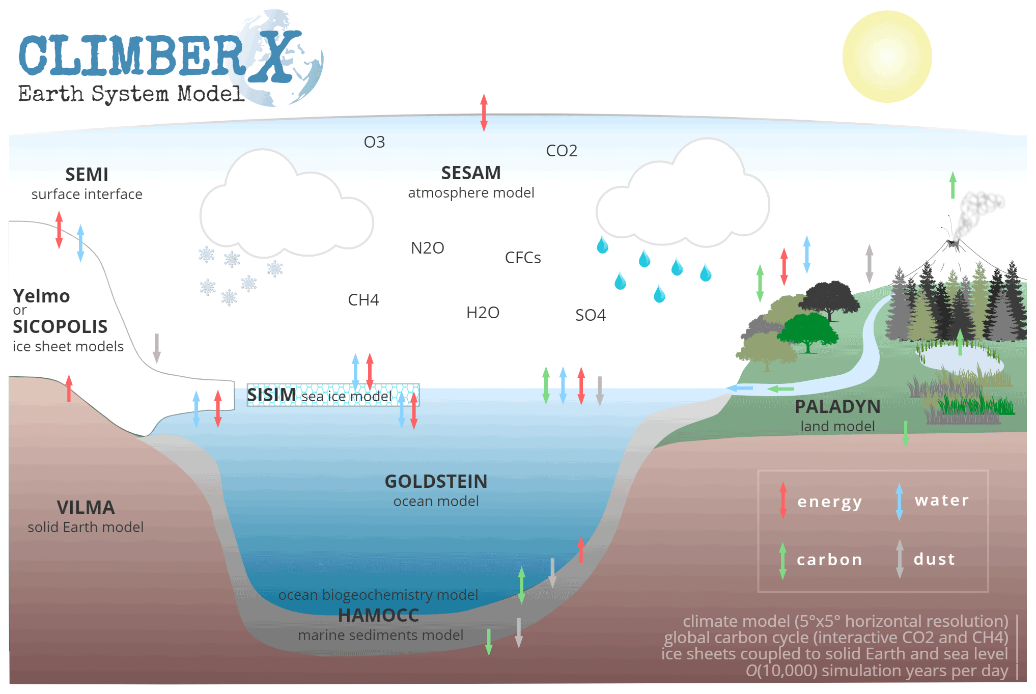
Figure 1 Schematic illustration of the CLIMBER-X model, including exchanges and coupling between the different modules.

In CLIMBER-X the land–ocean distribution, topography and land cover can evolve with time. A high-resolution (≈ 10 arcmin) topography input file is used to automatically generate the land–sea mask, the topography, the orographic roughness and the ocean bathymetry. For the present day the RTopo-2 data of Schaffer et al. (2016) are used. Runoff routing is also derived automatically from the high-resolution topography by following the steepest slope and using the algorithm of Planchon and Darboux (2002) to fill depressions. No manual intervention is needed in the process, so that CLIMBER-X can in principle also be applied for simulations of times in the past when the distribution of continents was very different from the present day. CLIMBER-X also allows for dynamic transient changes in the land–sea mask, which is important for simulations on long timescales, when sea-level changes or ice sheet expansion and retreat can cause substantial changes to the land and ocean areas, with important effects on the fluxes of energy and water between the surface and the atmosphere. Furthermore, because the model resolution is relatively coarse and the removal or addition of a whole cell could cause a large perturbation in the model, we have implemented land–sea fractions in each grid cell to ensure more continuous transitions. This fractional approach, common to many models, also increases the effective horizontal model resolution.

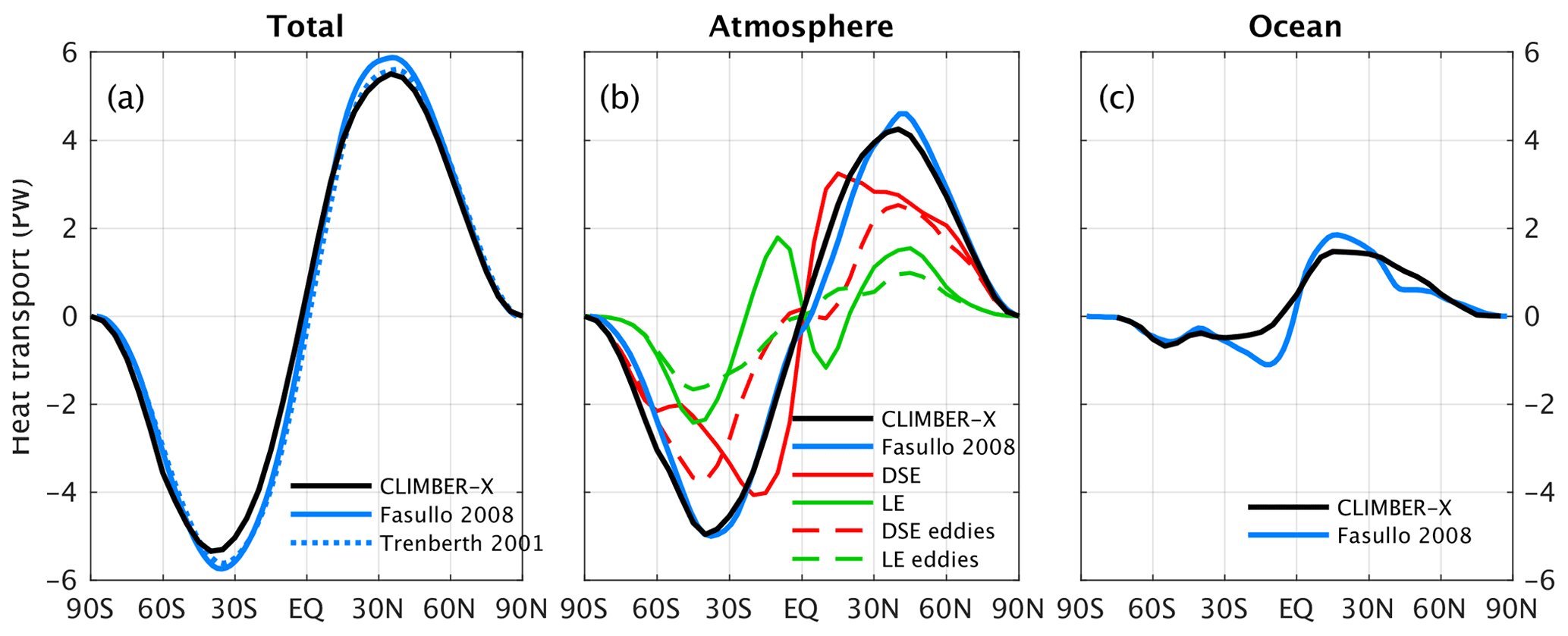
Figure 2 Meridional energy transport. (a) Total simulated meridional energy transport by ocean and atmosphere compared to observations (Trenberth and Caron, 2001; Fasullo and Trenberth, 2008). (b) Meridional energy transport by the atmosphere compared to estimates from Fasullo and Trenberth (2008) and modelled decomposition into dry static energy (DSE) and latent heat (LE) fluxes and contribution by eddies. (c) Global ocean meridional energy transport compared to observations (Fasullo and Trenberth, 2008).

CLIMBER-X is written entirely in Fortran 90+, making use of derived types to structure the single model components in a way which makes information transfer and exchange between different modules more transparent. The code is parallelized using the shared-memory OpenMP standard and integrates around 10 000 model years in 1 d on a single node with 2 × 8-core CPUs on a high-performance computer (Lenovo NeXtScale nx360M5, Xeon E5-2667v3 8C 3.2 GHz). The model is therefore ≈ 100–1000 times faster than state-of-the-art climate models that simulate weather when using comparable computational resources. Model input/output relies completely on the NetCDF data standard and uses the NCIO package (Robinson and Perrette, 2015) to read from and write to files. It therefore depends on the NetCDF library being available on the system where the model is run. Experimental settings and model parameters are defined in namelists, with one for each model component. A Python script is used to easily generate ensembles of simulations with different settings and parameters.

A conceptual overview of the individual model components is given in the following sections, while more details and equations are given in the Appendix.

2.1 Atmosphere model: SESAM

The atmospheric component of CLIMBER-X is designed as SESAM, based on a similar approach to the atmosphere of CLIMBER-2 (Petoukhov et al., 2000). Originally, the atmospheric component of CLIMBER-2 was positioned as a model based on equations derived (with some assumptions) from first principles. However, it has been found that the governing equations and some key parameterizations are hard to derive from first principles, and a number of modifications have been necessary to match results with observational data or results of more physically based models. This approach is explicitly and extensively used during the development of SESAM. Compared to CLIMBER-2, the new atmospheric component of CLIMBER-X has a much higher spatial resolution ($\mathrm{5}{}^{\circ }\times \mathrm{5}{}^{\circ }$), and most key parameterizations have been modified to improve performance against present-day climate and GCM sensitivity experiments. We made extensive use of available high-quality climatological data and results of complex climate model simulations which were not available when the CLIMBER-2 model was developed. This approach is reflected by the term “semi-empirical” in the model acronym.

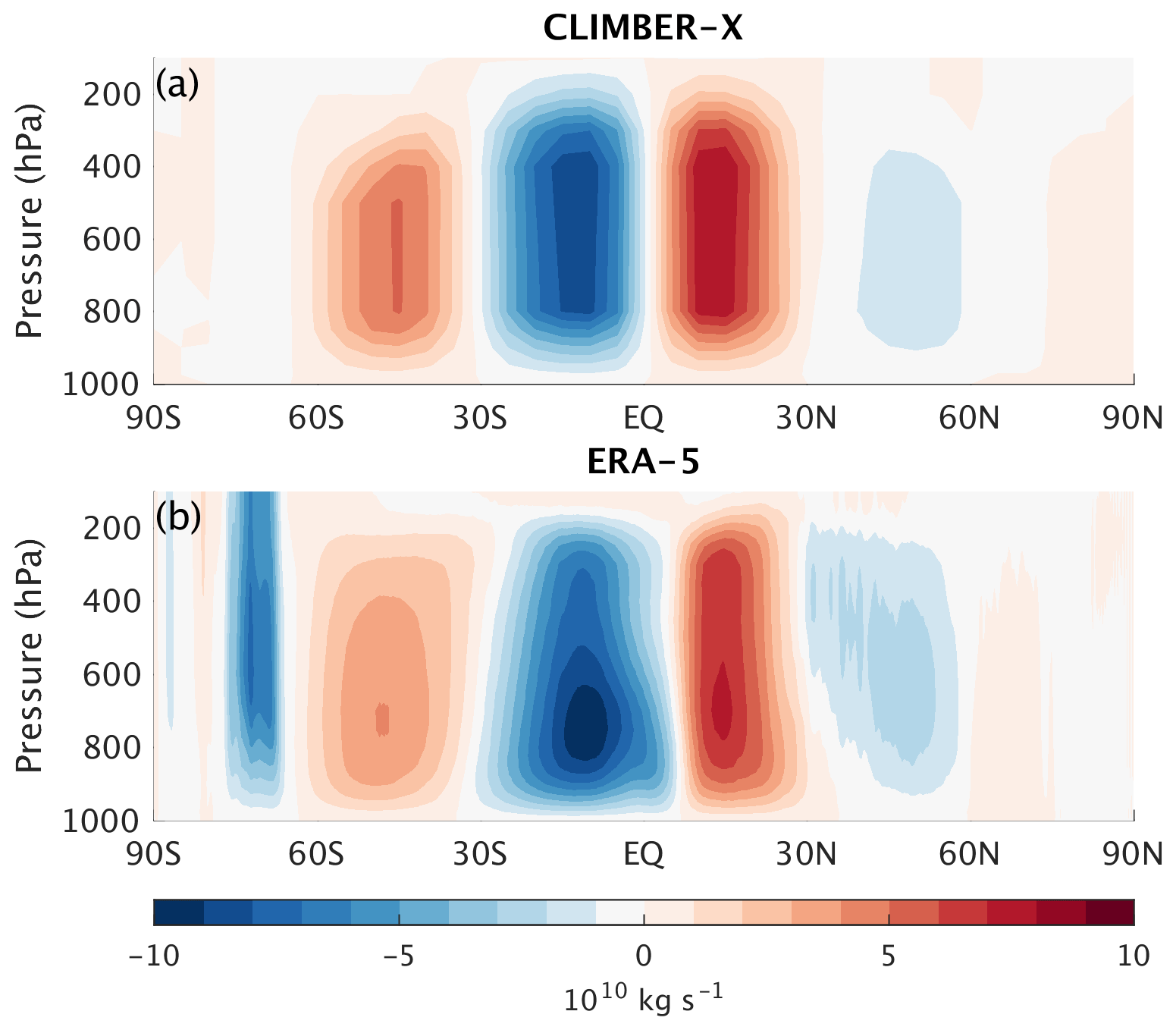
Figure 3 Annual mean (a) simulated meridional atmospheric streamfunction compared to (b) ERA-5 reanalysis (Hersbach et al., 2020).

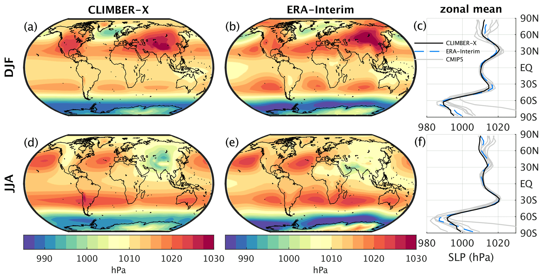
Figure 4 Sea-level pressure in CLIMBER-X for (a) DJF and (d) JJA compared to ERA-Interim reanalysis (Dee et al., 2011) (b, e). The zonal mean is additionally compared to CMIP5 models in panels (c) and (f).

The spatial resolution of SESAM, in terms of its representation of atmospheric fields, can be characterized as 2.5-D. This is related to the fact that, although prognostic variables (temperature, specific humidity, dust and eddy kinetic energy) as well as many diagnostic characteristics (cloudiness, condensation, shortwave radiation, etc.) are 2-D (latitude and longitude), the calculation of horizontal energy and water transport and the vertical fluxes of longwave radiation make use of information about the 3-D distribution of temperature, humidity, and wind velocity. All the vertical variations are purely diagnostic in the model. At the surface, each model grid cell is divided into different macro surface types, namely ocean, sea ice, land, lakes, and ice sheets. The macro surface types share the same atmospheric column but differ in surface elevation, albedo, and surface temperature and humidity. Sensible heat flux, evaporation, and shortwave and longwave radiation fluxes are computed separately for each macro surface type.

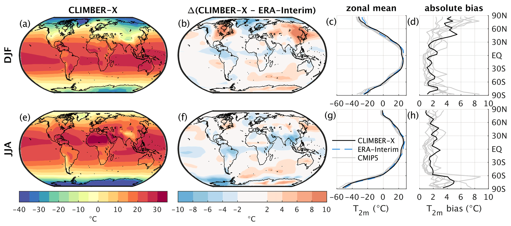
Figure 5 Near-surface air temperature in CLIMBER-X for (a) DJF and (e) JJA and model bias relative to ERA-Interim reanalysis (Dee et al., 2011) (b, f). The zonal mean is additionally compared to CMIP5 models in panels (c) and (g). The zonal mean absolute model bias in CLIMBER-X and a selection of CMIP5 models relative to ERA-Interim are shown in panels (d) and (h) for DJF and JJA, respectively.

The 3-D atmospheric structure is derived using assumptions about the universal vertical structure of temperature and relative humidity in the atmosphere. The temperature profile through the troposphere is a quadratic function of height, except in a 1500 m layer close to the surface where the lapse rate is a function of the near-surface atmospheric stability. Inversion strength is determined by the surface radiative balance and the difference between near-surface air temperature and skin temperature. Temperature is vertically uniform in the stratosphere. The tropopause height is derived assuming that the stratosphere is in radiative equilibrium. Relative humidity is taken to be constant within the planetary boundary layer, to decay exponentially in the low troposphere and to remain constant throughout the rest of the troposphere. Stratospheric relative humidity is prescribed at a uniform constant value. This approach differs from that used in CLIMBER-2, where specific humidity profiles were prescribed instead of relative humidity. This can lead to large biases in relative humidity in the mid–upper troposphere, where humidity is important for its effect on longwave radiation. Therefore, in SESAM the vertical profile of relative humidity is parameterized instead. See Appendix A1 for more details on the parameterization of the vertical structure.

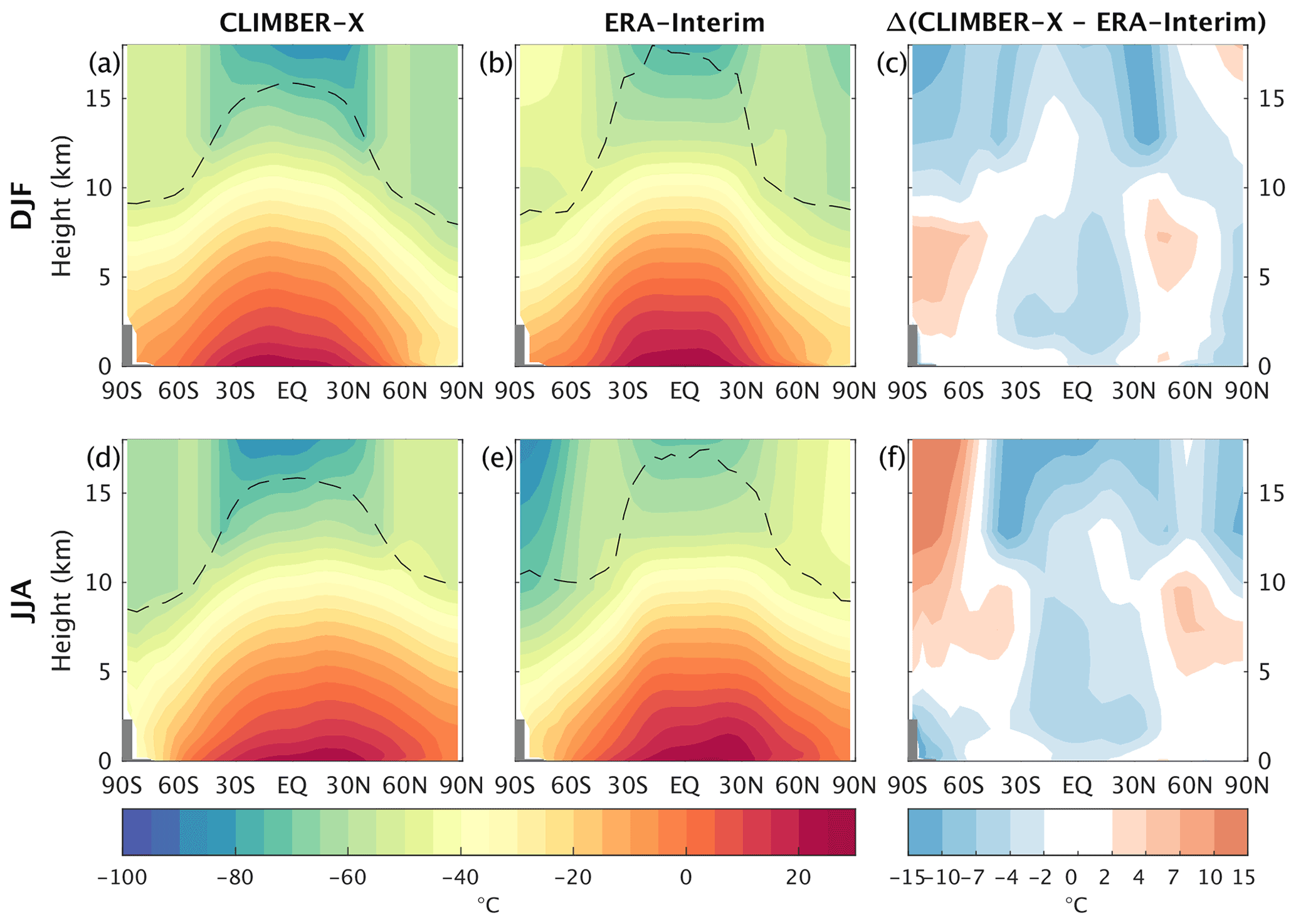
Figure 6 Zonal mean temperature simulated by CLIMBER-X for (a) DJF and (d) JJA compared to ERA-Interim reanalysis (Dee et al., 2011) (b, e). The temperature bias relative to ERA-Interim is shown in panels (c) and (f). The dashed black line indicates the height of the tropopause.

Figure 7 Near-surface air temperature seasonality in (a) CLIMBER-X compared to (b) ERA-Interim reanalysis (Dee et al., 2011) computed as the difference between maximum and minimum monthly temperature.

Similarly to CLIMBER-2, in SESAM the horizontal wind velocity is divided into geostrophic and ageostrophic components. The geostrophic components of velocity at sea level are computed from sea-level pressure (SLP) and at any height through the troposphere by using the thermal wind approximation. The components of the surface wind are computed using the Taylor model (see e.g. Hansen et al., 1983). The ageostrophic wind components in the planetary boundary layer are computed from the SLP gradient and the cross-isobar angle. SLP is the sum of zonally averaged and azonal components. The zonal component of SLP is derived based on the assumption that the strength and position of the major cells of the atmospheric meridional overturning circulation are controlled by average meridional temperature gradients and zonally averaged surface drag, similarly to Petoukhov et al. (2000). An additional dependence on zonal mean surface elevation has been added in SESAM to account for the effect of topography. The zonally averaged SLP is directly related to the zonal mean meridional (ageostrophic) wind in the planetary boundary layer and therefore the mean meridional circulation. The vertical structure of the zonally averaged meridional circulation is parameterized following the approach of Petoukhov et al. (2000). The azonal component of mean SLP resulting from stationary planetary waves is separated into a thermal component and an orographic component. The thermal component is assumed to be proportional to the azonal surface temperature anomaly reduced to sea level using the interrelation between long-term large-scale azonal temperature and pressure in quasi-stationary planetary-scale waves, similarly to Petoukhov et al. (2000). The effect of topographic stationary waves is particularly important for the Northern Hemisphere (NH) mid-latitude winter. The simple 1-D barotropic model for forced topographic Rossby waves of Charney and Eliassen (1949), applied to each latitudinal belt separately, is used to account for this effect in SESAM. Note that in CLIMBER-2 topographic waves were not represented because of the low spatial model resolution, whereas this limitation does not exist for CLIMBER-X. The main limitation in atmospheric dynamics in SESAM lies in the employed geostrophic approximation, which is not valid close to the Equator, resulting in deficiencies in the simulated dynamics in the tropics. See Appendix A2 for more details on the model dynamics.

SESAM includes a prognostic equation for vertically integrated energy and another for total-column water content, from which surface air temperature and humidity are derived. Sources and sinks of energy in the column include net longwave and shortwave radiation, surface sensible heat flux and latent heat release from condensation. Sources and sinks of water in the column are given by surface evaporation and precipitation. The 3-D wind field is used to advect the 3-D potential temperature field and 3-D specific humidity fields. Horizontal transport due to synoptic-scale processes is described as macroturbulent diffusion with an isotropic coefficient of horizontal diffusion expressed through the eddy kinetic energy (EKE). Precipitation is generated in the model whenever near-surface air relative humidity exceeds a critical threshold of 95 %. The water excess is then instantaneously added to precipitation. Over land, precipitation is additionally generated from column water content with a specified turnover time that is inversely proportional to atmospheric relative humidity. See Appendices A3 and A4 for more details on the energy and water balance equations.

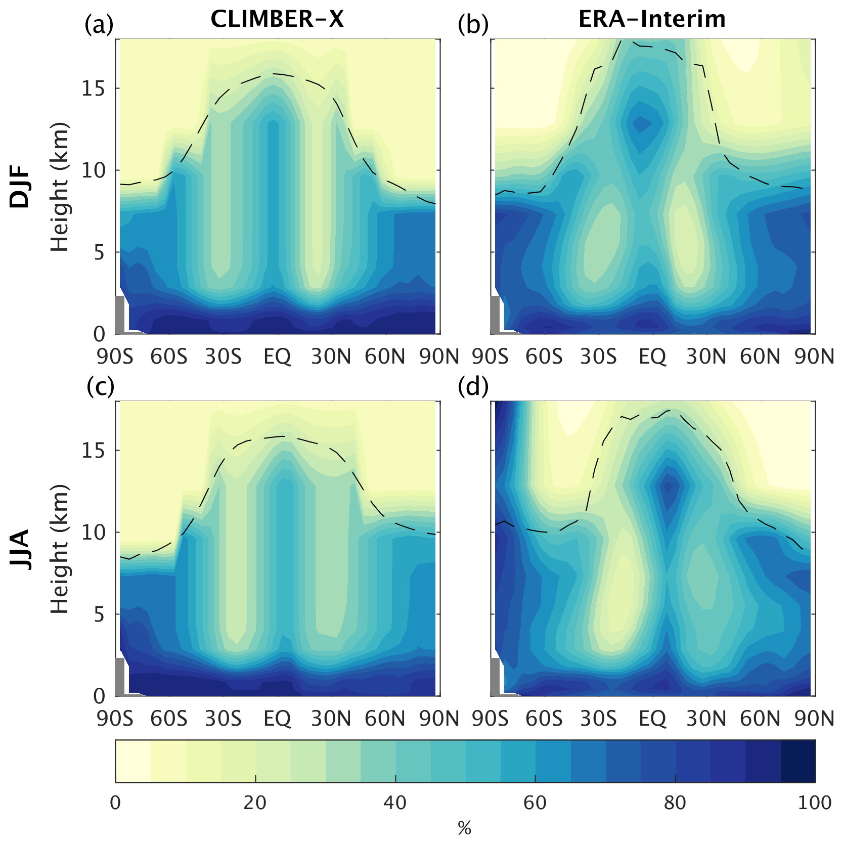
Figure 8 Zonal mean relative humidity simulated by CLIMBER-X for (a) DJF and (c) JJA compared to ERA-Interim reanalysis (Dee et al., 2011) (b, d). The dashed black line indicates the height of the tropopause.

Figure 9 Precipitation modelled by CLIMBER-X for (a) DJF and (d) JJA compared to ERA-Interim reanalysis (Dee et al., 2011) (b, e). The zonal mean is additionally compared to CMIP5 models in panels (c) and (f).

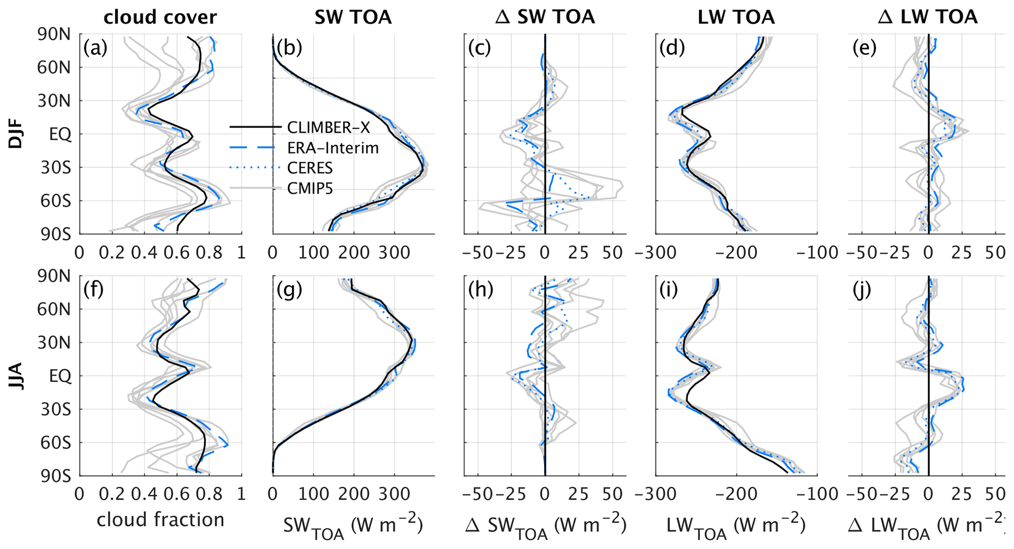
Figure 10 Simulated zonal mean cloud fraction and top-of-the-atmosphere net radiation fluxes for (top) DJF and (bottom) JJA compared to satellite observations (Loeb et al., 2018), reanalysis (Dee et al., 2011), and CMIP5 models.

The (vertically integrated) EKE is a prognostic variable in the model. EKE production is proportional to the baroclinicity of the atmosphere as defined by the Eady baroclinicity measure (e.g. Hoskins and Valdes, 1990). EKE dissipation depends on the surface aerodynamic drag coefficient and is proportional to ${\mathrm{EKE}}^{\mathrm{3}/\mathrm{2}}$. EKE is itself transported by macroturbulent diffusion and advected by the wind at 700 hPa. The synoptic component of surface wind speed is then taken to be proportional to $\sqrt{\mathrm{EKE}}$. See Appendix A5 for more details on the model representation of synoptic processes.

SESAM includes a single effective cloud layer. In this respect it is therefore even simpler than CLIMBER-2, which separately treats stratiform and convective clouds. We did not find any advantages in a separate treatment of different types of clouds in the framework of our modelling approach. Cloud fraction is a function of atmospheric relative humidity, effective vertical velocity and near-surface temperature inversion strength. Cloud top height is related to the height of the troposphere, modified by a factor depending on the vertical velocity at the cloud base. Cloud optical thickness is a function of surface air temperature, cloud fraction, column water content and sulfate aerosol load. Since CLIMBER-X does not include an atmospheric chemistry module, the spatial distribution of sulfate aerosol load must be prescribed as input to the model. See Appendix A6 for more details on cloud parameterizations.

The shortwave radiation scheme accounts for water vapour, clouds, sulfate aerosols, dust and ozone. The total shortwave radiation range is divided into two subintervals: ultraviolet + visible and near-infrared. The cloud albedo is a function of solar zenith angle and the optical thickness of the clouds (Feigelson et al., 1975). The optical properties of dust are treated following the Yamamoto and Tanaka (1972) scheme. The integral transmission function of ozone is taken from Lacis and Hansen (1974). In the near-infrared band the absorption due to water vapour is described according to Feigelson et al. (1975). The effect of sulfate aerosols is included following the approach of Bauer et al. (2008). The scheme accounts for both the direct radiative forcing and the indirect effect through changes in cloud optical thickness. For simplicity, the radiative effect of black carbon and organic carbon aerosols is not represented in the model, as it is implicitly assumed that their combined net effect is negligible to a first approximation. See Appendix A7 for more details on shortwave radiation.

Figure 11 Simulated ocean overturning circulation: (a) global and (b) Atlantic.

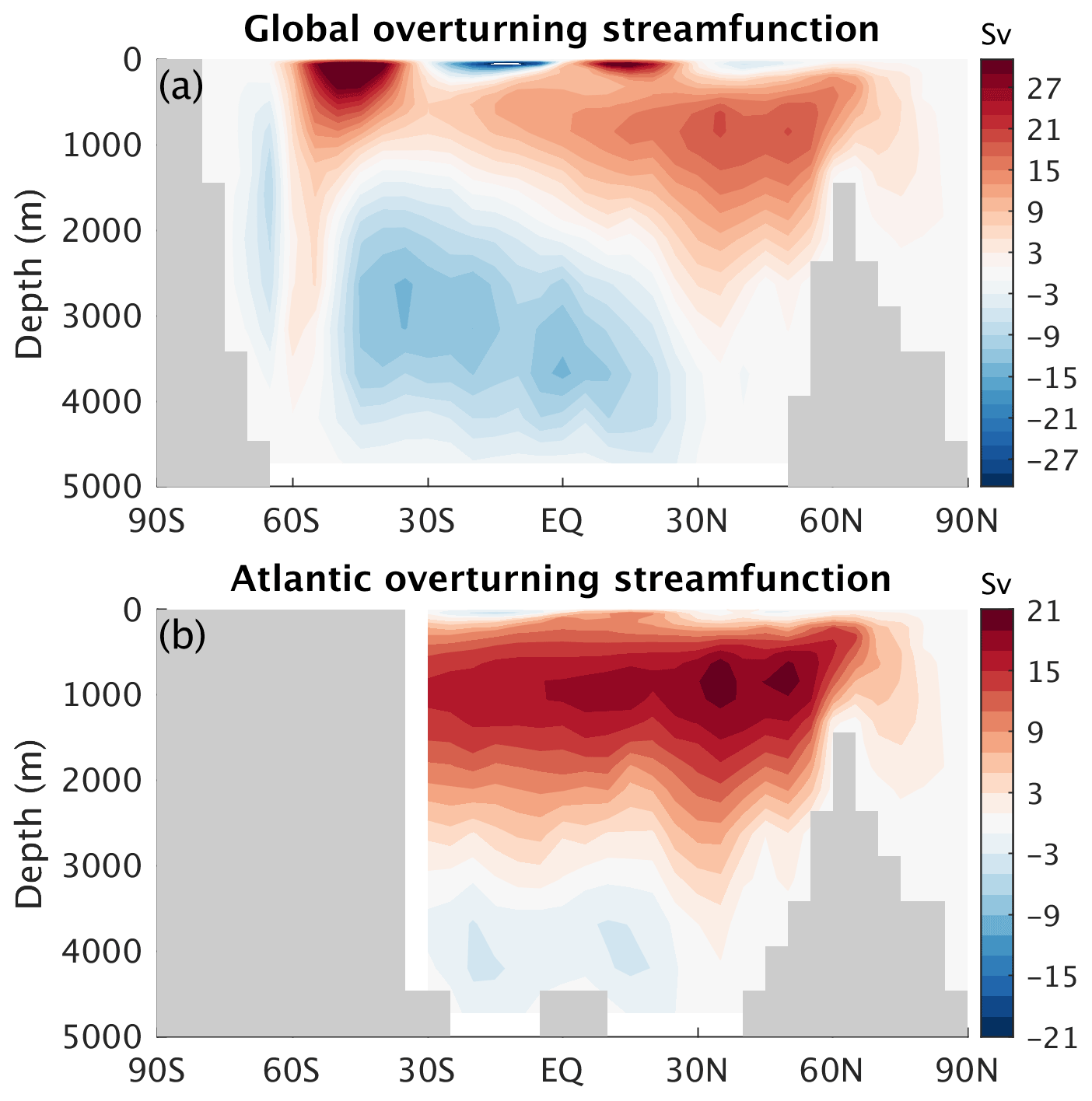
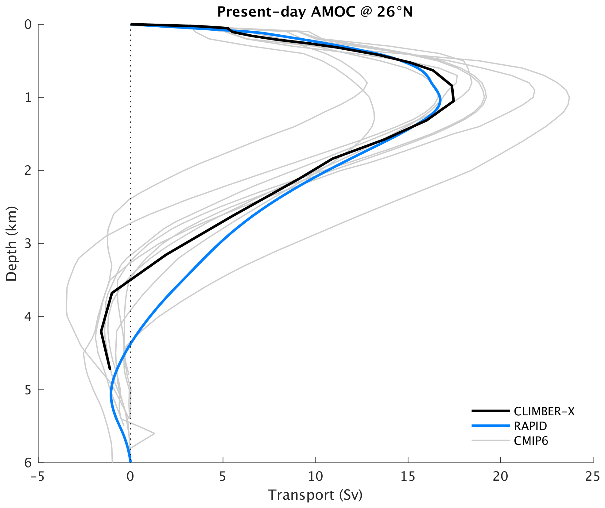
Figure 12 Vertical profile of the simulated Atlantic meridional overturning streamfunction at 26^∘ N (black) compared to observations from the RAPID array (Frajka-Williams et al., 2021) (blue) and a selection of CMIP6 models (grey). The CLIMBER-X and CMIP6 streamfunction is computed from historical simulations as the average over the time period from 2000 to 2014, while the RAPID values represent an average from 2004 to 2020.

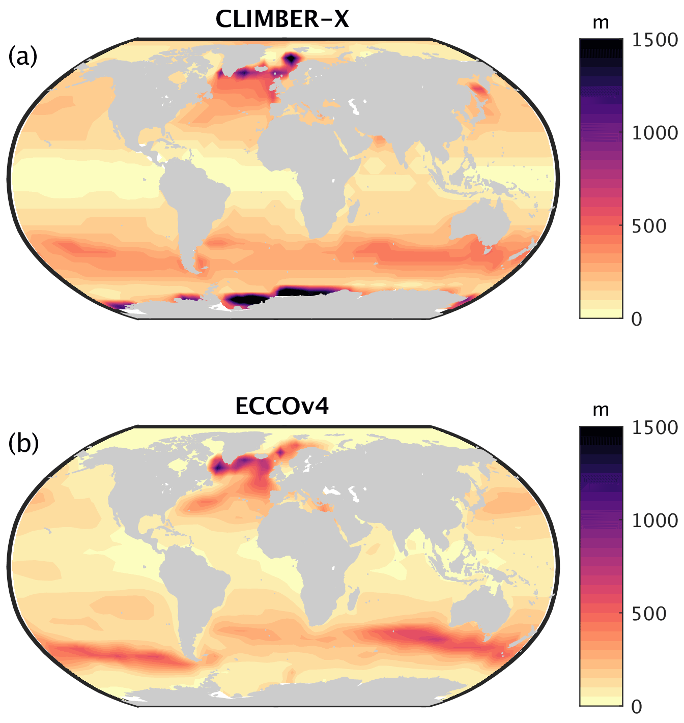
Figure 13 Maximum monthly mixed-layer depth simulated by CLIMBER-X (a) compared to ECCOv4 reanalysis (ECCO Consortium et al., 2021) (b).

To compute the longwave radiation fluxes, the atmosphere column is subdivided into 15 unevenly spaced levels. The longwave radiative scheme accounts explicitly for water vapour, carbon dioxide, and ozone through their integral transmission functions. The longwave radiative effect of the well-mixed greenhouse gases CH₄, N₂O and CFCs is accounted for through the use of an equivalent CO₂ concentration in the radiative scheme, using the respective radiative forcing following Etminan et al. (2016). Similarly to sulfate aerosols, the 3-D field of ozone concentration must be prescribed as input to the model. It can be time-dependent. See Appendix A8 for more details on longwave radiation.

A simple representation of the global dust cycle is included in SESAM based on a single representative dust particle diameter (Bauer and Ganopolski, 2010). Dust emissions are computed in the land model and are an input to the atmosphere, where the dust concentration is assumed to decrease exponentially with height with a fixed height scale of 2 km. Dust is transported by the 3-D wind field and by macroturbulent diffusion. Dust sinks include both dry and wet deposition.

Figure 14 Zonal mean ocean temperature simulated by CLIMBER-X (a, d, g) compared to WOA13 data (Levitus et al., 2015) (b, e, h) for the (a, b, c) Atlantic, (d, e, f) Pacific, and (g, h, i) Indian and Southern oceans. Panels (c), (f), and (i) show the model bias.​​​​​​​

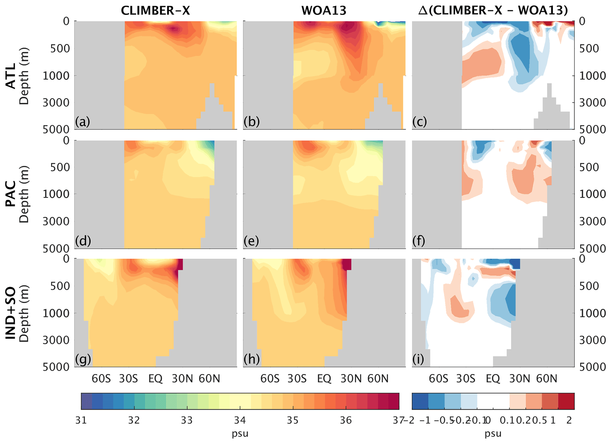
Figure 15 Zonal mean ocean salinity simulated by CLIMBER-X (a, d, g) compared to WOA13 data (Levitus et al., 2015) (b, e, h) for the (a, b, c) Atlantic, (d, e, f) Pacific, and (g, h, i) Indian and Southern oceans. The right panels show the model bias.

2.2 Ocean model: GOLDSTEIN

The ocean component of CLIMBER-X is based on GOLDSTEIN (Edwards et al., 1998; Edwards and Shepherd, 2002; Edwards and Marsh, 2005). GOLDSTEIN is a 3-D frictional–geostrophic balance model and is also employed in several other existing EMICs, e.g. GENIE (Marsh et al., 2011) and Bern3D (Müller et al., 2006). In the original GOLDSTEIN implementation, the equations were coded in terms of non-dimensional quantities. For the inclusion in CLIMBER-X, the code has been dimensionalized for better readability and more efficient debugging.

The horizontal velocity in the ocean is diagnosed from a frictional–geostrophic balance and the vertical velocity is then derived from the continuity equation. The model assumes hydrostatic balance. The velocity relaxation to the velocities of the previous time step employed in GENIE and Bern3D has been removed in CLIMBER-X without drawbacks for model stability. Islands for barotropic flow are automatically derived from the topography, but the actual islands around which barotropic flow is permitted can be controlled by namelist settings. By default, non-zero barotropic flow is allowed through the Drake Passage and through the Indonesian archipelago. The Bering and Davis straits are closed for barotropic flow, but baroclinic tracer exchange is permitted. The friction for baroclinic velocities is set to be 4 d⁻¹ and is globally uniform, while the friction for barotropic velocities is increased by a factor of 3 near continental boundaries and shallow topographic features. Close to the Equator the minimum absolute value of the Coriolis parameter is set to $\mathrm{5}\times {\mathrm{10}}^{-\mathrm{6}}$ s⁻¹. In contrast to other models using GOLDSTEIN (e.g. Holden et al., 2016; Marsh et al., 2011; Müller et al., 2006) in CLIMBER-X, the wind stress as simulated by the atmospheric model is applied at the ocean surface, without any enhancement factor. Seawater density is computed using the UNESCO equation of state of Millero and Poisson (1981).

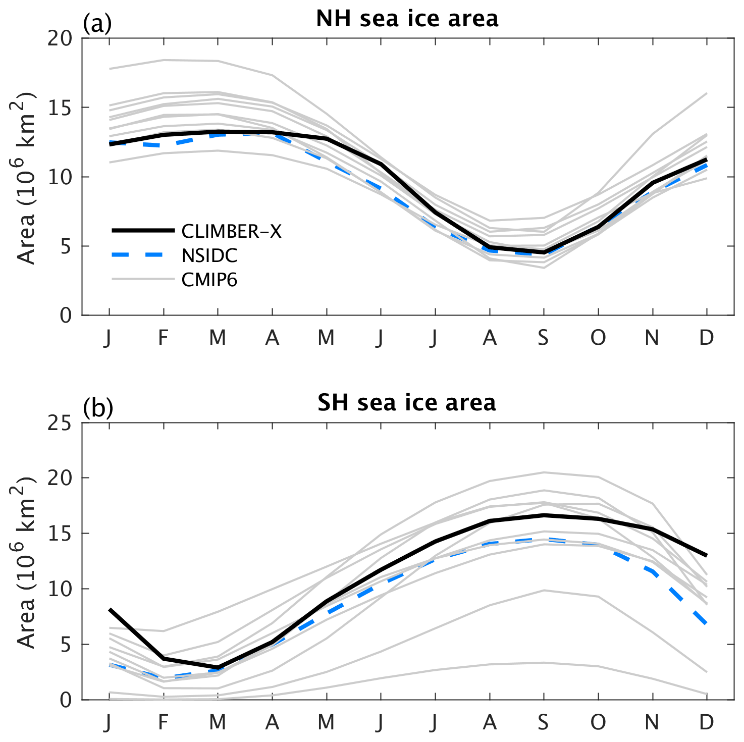
Figure 16 Seasonal variation of total sea ice area for (a) the NH and (b) the SH as simulated by CLIMBER-X (black) compared to observations (Meier et al., 2021) (blue) and CMIP6 models (grey).

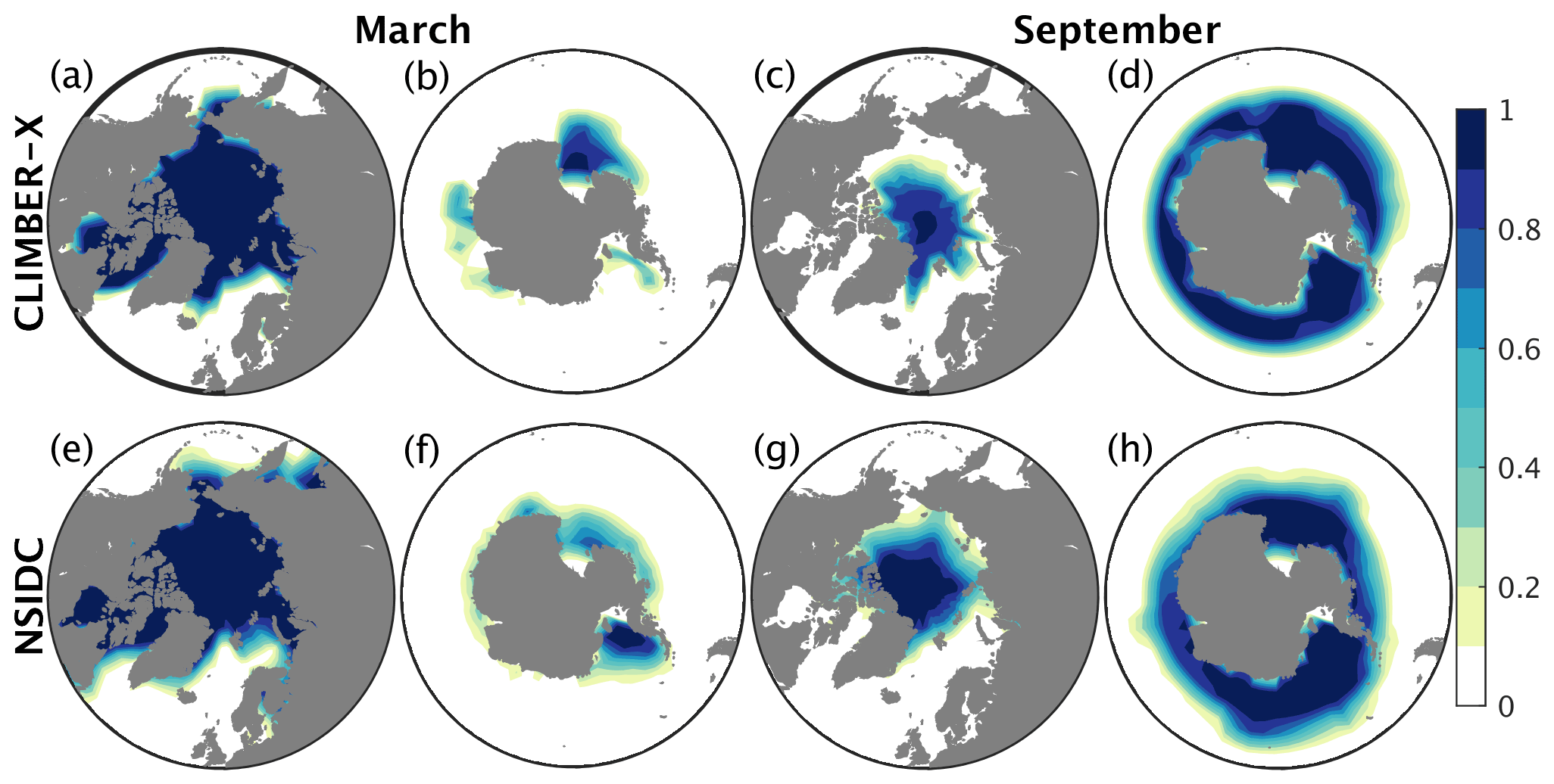
Figure 17 Sea ice concentration in the NH and SH in CLIMBER-X (top) compared to observations (Meier et al., 2021) (bottom) for (left) March and (right) September.

The principal limitations to the ocean dynamics follow from reduced resolution and the neglect of non-linear momentum advection. The result is that there are no ocean eddies and hence no mechanism for internally generated variability and that boundary currents are unrealistically broad. One notable consequence of the strong momentum damping is a generally weak Antarctic Circumpolar Current and Gulf Stream. See Edwards and Marsh (2005) and Müller et al. (2006) for a more detailed discussion of the limitations of the frictional–geostrophic dynamics.

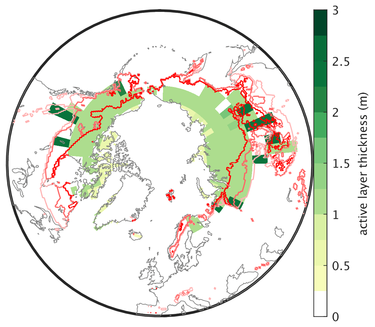
Figure 18 Modelled permafrost extent and active layer thickness compared to the observed extent of continuous, discontinuous, and isolated permafrost (red lines, from dark red to light red) from Brown et al. (1998). The active layer thickness is calculated as the mean over the period 1981–2010 in grid cells that are permafrost during the whole time period.

The tracer transport is described by an advection–diffusion equation, written in flux form. To reduce numerical diffusion associated with the original advection scheme, we have implemented a flux-corrected transport scheme following Zalesak (1979). The model uses an explicit isopycnal and diapycnal diffusion scheme in its small-angle approximation (Redi, 1982) combined with a diffusive parameterization of the eddy-induced transport following the Gent–McWilliams skew flux (Gent and Mcwilliams, 1990; Griffies, 1998). The coefficients for both eddy-induced transport and isopycnal mixing are assumed to be equal by default (1500 m²s⁻¹). Slopes of the isoneutral surfaces above $\mathrm{1}\times {\mathrm{10}}^{-\mathrm{3}}$ are tapered following Gerdes et al. (1991). The diapycnal diffusivity profile follows Bryan and Lewis (1979) with a minimum diffusivity of 0.1 cm² s⁻¹ at the surface and a maximum of 1.5 cm² s⁻¹ at the ocean floor. If the stratification of a water column is statically unstable, convective adjustment is applied using the scheme of Rahmstorf (1993). A simple mixed-layer scheme, based on Kraus and Turner (1967), is used in the model. Heat and freshwater fluxes at the ocean surface provide the top boundary conditions for the temperature and salinity prognostic equations. Since GOLDSTEIN is based on the rigid-lid approximation, the freshwater flux is implemented in terms of a virtual salinity flux, computed using local salinity. A global correction is employed to ensure that the global annual net freshwater flux into the ocean is zero, in the absence of changes in land ice volume. This is not sufficient to ensure conservation of salinity in the ocean because of the anti-correlation between surface freshwater flux and surface salinity (e.g. Yin et al., 2010). Hence, the virtual salinity flux is additionally corrected to ensure that the annual mean global net surface flux is zero. The geothermal heat flux of Lucazeau (2019) is applied as a bottom ocean boundary condition.

The model is discretized on a regular lat–long grid with $\mathrm{5}{}^{\circ }\times \mathrm{5}{}^{\circ }$ resolution, matching the atmosphere model resolution, and 23 unequally spaced vertical layers, with a 10 m top layer and layer thickness increasing with depth and reaching 500 m at the ocean bottom. Ocean bathymetry is smoothed by convolving bathymetry with a directly neighbouring four-grid-point kernel to remove strong gradients that would lead to numerical instabilities. To improve model stability, an additional limitation on the topographic slope entering in the Coriolis term (planetary vorticity advection) of the barotropic velocity equation is applied.

Since the land–sea mask is fully flexible in CLIMBER-X, GOLDSTEIN has been adapted to deal with newly forming and disappearing oceanic grid cells. It is always ensured that all grid cells of the ocean domain are connected. If “ocean lakes” are formed at any point in time, the isolated ocean cells are removed from the ocean model domain and are treated as lake in the land model instead. A minimum ocean fraction of 0.1 in a $\mathrm{5}{}^{\circ }\times \mathrm{5}{}^{\circ }$ grid cell is required for a cell to be considered part of the ocean domain. Newly formed cells are initialized using information from neighbouring grid cells. Changes in sea level, and therefore ocean volume, are additionally accounted for by scaling the thicknesses of the ocean layers below a depth of 1000 m to match the actual ocean volume derived from the high-resolution topography and provided as input to the ocean model. Total tracer inventories in the ocean are conserved in this process. Islands for barotropic flow are automatically updated with the mask. Velocities are diagnostic quantities in the model, and therefore no intervention on velocity fields is required when updating the land–sea mask.

Information on sea surface height is needed in the sea ice momentum equation. The rigid-lid formulation employed in GOLDSTEIN does imply a surface pressure (e.g. Pinardi et al., 1995), the so-called rigid-lid pressure, which is directly related to the sea surface height. However, instead of solving the non-trivial equation for surface pressure, in the model an approximate approach is used in which surface pressure is simply diagnosed from integrating density above a reference depth of 1500 m.

Additional tracers, including CFCs, dye and age tracers, have been added to the model as useful diagnostics. The air–sea fluxes of CFCs are computed following the Ocean Model Intercomparison Project (OMIP) protocol (Orr et al., 2017).

Additional details of the ocean model are provided in Appendix B.

Figure 19 (a) Historical global mean near-surface air temperature simulated by CLIMBER-X (black) compared to observations (blue) (Morice et al., 2012) and CMIP6 models (grey). (b–d) Global mean near-surface air temperature in CLIMBER-X and CMIP6 models for idealized historical simulations with greenhouse gas concentration forcing only, natural (solar and volcanic) forcing only, and aerosol forcing only, respectively.

2.3 Sea ice model: SISIM

SISIM is a dynamic–thermodynamic sea ice model, with a single ice layer and a snow layer on top. SISIM also serves as a coupler between the atmosphere and ocean, and hence all surface energy fluxes over both sea ice and open ocean are computed in the sea ice model.

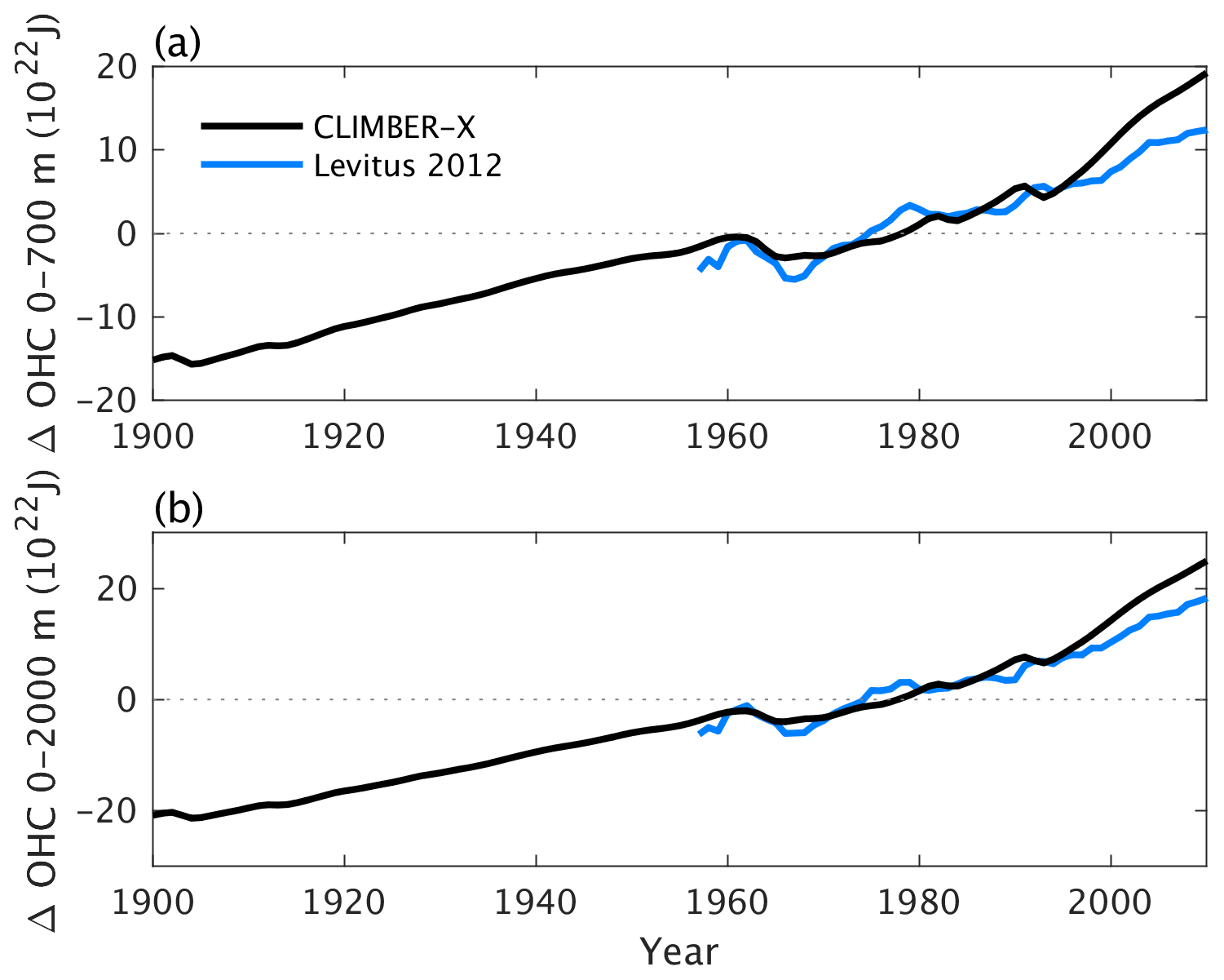
Figure 20 Historical ocean heat content anomalies in (a) the top 700 m and (b) the top 2000 m simulated by CLIMBER-X (black) and derived from observations (blue) (Levitus et al., 2012).

Sea ice thermodynamics are based on the zero-layer model of Semtner (1976). This involves the determination of accumulation and melting of snow/sea ice from above and accretion and melting of sea ice from below.

The surface energy balance equation is solved separately for the ice-free and ice-covered areas of each oceanic grid cell. Over sea ice, it is solved implicitly for the skin temperature, which is the temperature that balances all energy fluxes at the surface. The fluxes to be balanced include the net shortwave and longwave radiation at the surface, the sensible and latent heat fluxes to the atmosphere and the conductive heat flux into the snow/ice. Whenever the skin temperature over the snow/sea ice layer is above the melting point, the skin temperature is reset to 0 ^∘C and the excess energy is used to melt snow/sea ice. Snowfall increases snow thickness, and if the snow depth exceeds 1 m, the snow excess is converted to sea ice. The net energy at the base of the ice layer is determined by the conductive heat flux through the snow/ice layer and the turbulent heat flux between the ice and the seawater below. Whether accretion or ablation occurs depends on the sign of the net energy at the ice–water interface. Over seawater, the heat flux into the ocean is computed as the residual of the radiation and surface energy fluxes, whereby the surface energy fluxes are computed using sea surface temperature. Sea ice forms whenever the top-layer ocean temperature drops below the freezing point of seawater.

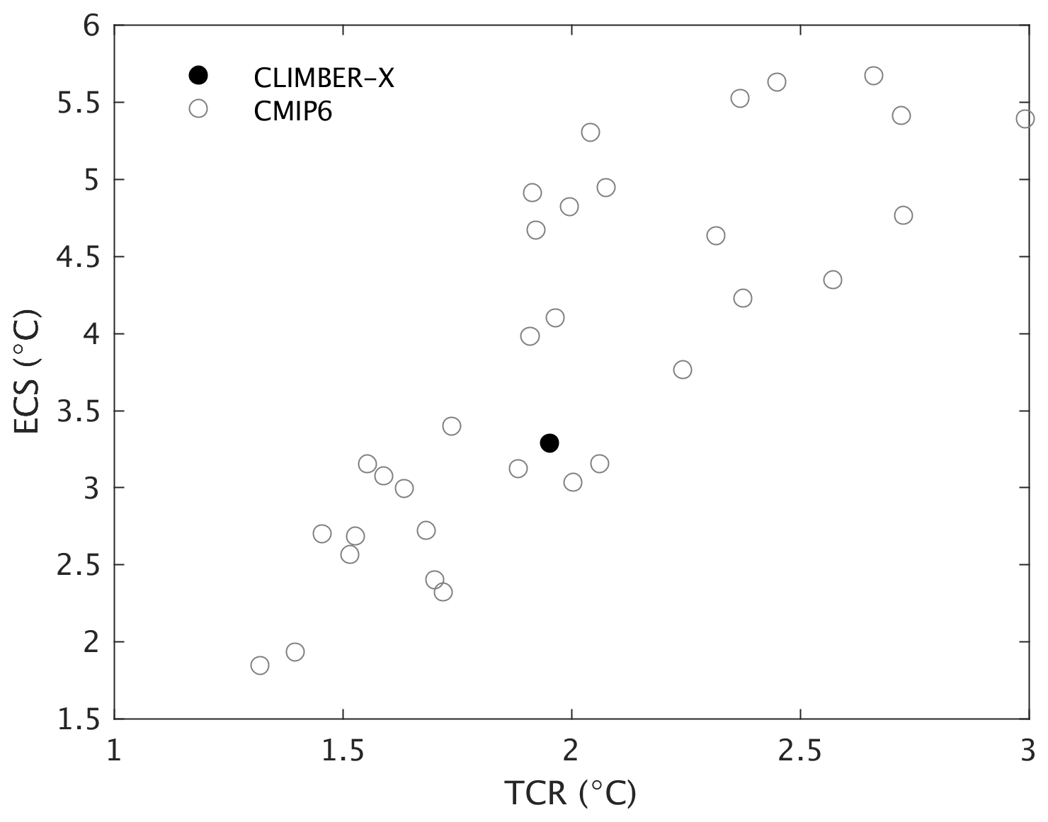
Figure 21 Equilibrium climate sensitivity versus transient climate response for the CLIMBER-X and CMIP6 models. CMIP6 model data are from Nijsse et al. (2020).

The surface sensible and latent heat fluxes are proportional to the temperature and moisture gradients between the surface and near-surface air, with the exchange coefficients depending on atmospheric stability through a bulk Richardson number. Sea ice albedo is temperature-dependent, with a decrease in albedo as the sea ice skin temperature approaches the melting point. This represents the decrease in albedo following the formation of meltwater ponds on the ice surface. The snow albedo scheme is the same as used in the land model and includes a dependence on snow grain size and dust and soot concentration following Dang et al. (2015). The conductive heat flux within the sea ice/snow layer is assumed to be directly proportional to the temperature difference between the surface skin and the salinity-dependent freezing temperature at the base of the ice layer (Semtner, 1976). The sea ice heat conductivity is scaled to represent sub-grid thickness distribution following Fichefet and Maqueda (1997). The turbulent heat flux at the ice base is determined from the difference between salinity-dependent freezing point temperature and top-layer ocean temperature using a constant exchange coefficient following McPhee (1992) and Weaver et al. (2001).

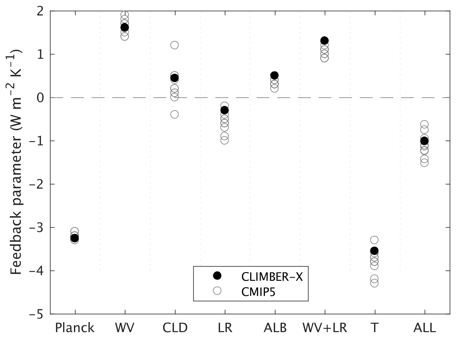
Figure 22 Global feedback parameters for the CLIMBER-X and CMIP5 models. The feedbacks are (from left to right) Planck, water vapour, cloud, lapse rate, albedo, water vapour + lapse rate, temperature (Planck + lapse rate), and the sum of all feedbacks. CMIP5 data are from IPCC AR5.

Sea ice drift velocities are computed from the momentum balance equation (e.g. Hibler, 1979) with the elastic–viscous–plastic rheology of Hunke and Dukowicz (1997) and Bouillon et al. (2009). Numerically the solution of the momentum equation follows the implementation in GFDL model SIS2 (Adcroft et al., 2019; Delworth et al., 2006), discretized on the Arakawa C grid to match the ocean model grid. The derived velocities are then used to advect the grid cell mean ice and snow thicknesses and the sea ice concentration using a flux-corrected transport scheme (Zalesak, 1979). No explicit diffusion is applied.

Sea ice is allowed to cover the ocean fraction of the grid cell that is not occupied by shelf ice. That is, floating shelf ice restricts the domain available to sea ice.

Additional details of the sea ice model are provided in Appendix C.

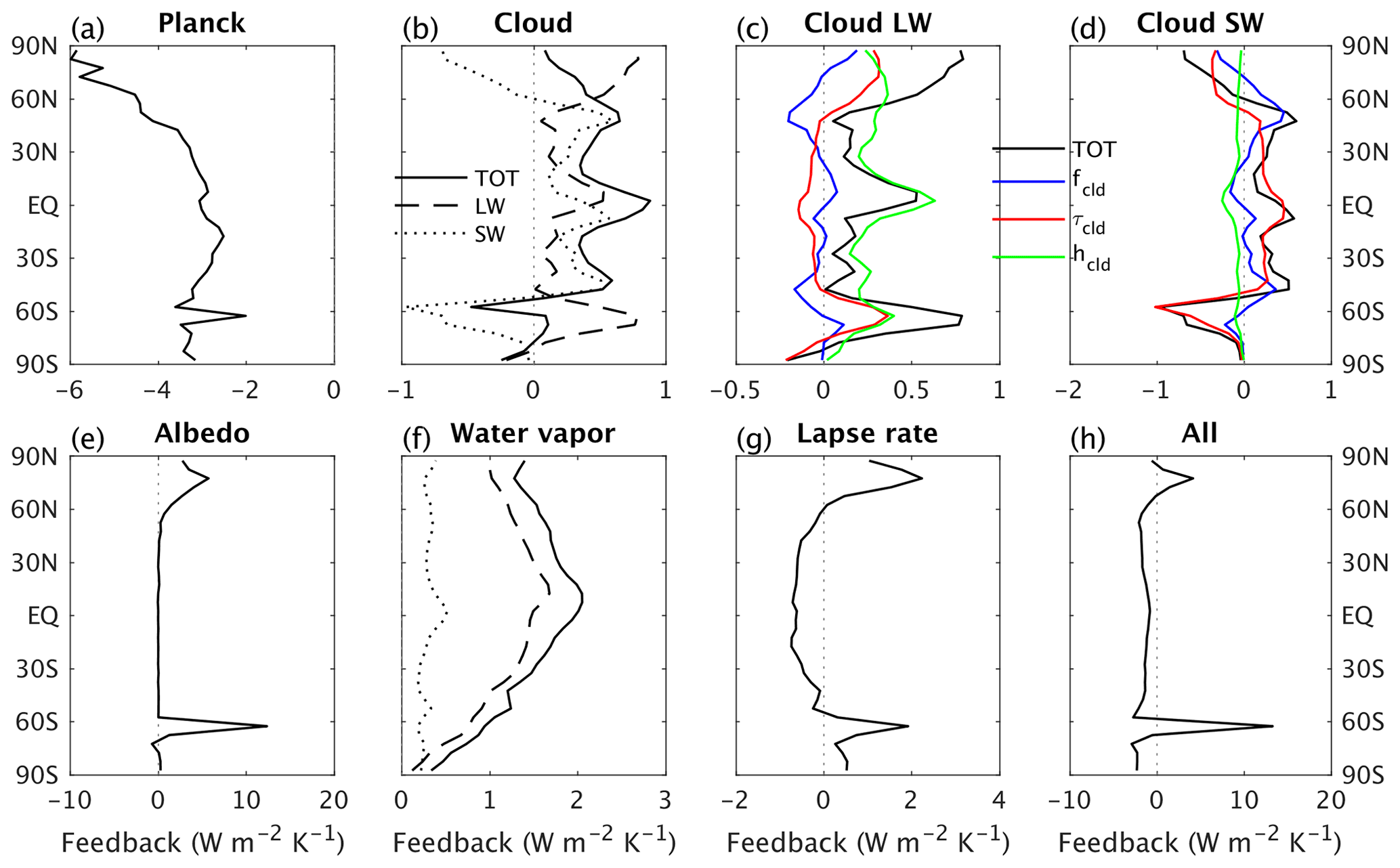
Figure 23 Zonal mean feedback parameters for CLIMBER-X. The total feedbacks (black solid lines) are further separated into contributions from longwave (LW, dashed black lines) and shortwave (SW, dotted black lines) radiation. Cloud feedbacks are additionally explicitly decomposed into LW and SW in panels (c) and (d), with the different colours representing feedbacks from changes in cloud fraction (blue), cloud optical thickness (red), and cloud top height (green).

2.4 Land model: PALADYN

CLIMBER-X includes the land model PALADYN (Willeit and Ganopolski, 2016), which serves as a land surface scheme for the exchange of energy and water between the surface and the atmosphere but also represents vegetation dynamics and, more generally, the land carbon cycle processes. The model treats in a consistent manner the interaction between atmosphere, terrestrial vegetation and soil through the fluxes of energy, water and carbon. Permafrost is treated explicitly, both in physical processes and as an important carbon pool. PALADYN distinguishes eight surface types, namely five plant functional types, bare soil, land ice and lakes. Over each surface type the model solves the surface energy balance and computes the fluxes of sensible, latent and ground heat and upward shortwave and longwave radiation. It includes a single snow layer. Vegetation and bare soil share a single soil column. The soil is vertically discretized into five layers where prognostic equations for temperature, water and carbon are consistently solved. Phase changes of water in the soil are explicitly considered. A surface hydrology module computes precipitation interception by vegetation, surface runoff and soil infiltration. The soil water equation is based on Darcy's law. Given soil water content, the wetland fraction is computed based on a topographic index. Modifications to the model relative to the description in Willeit and Ganopolski (2016) are described next.

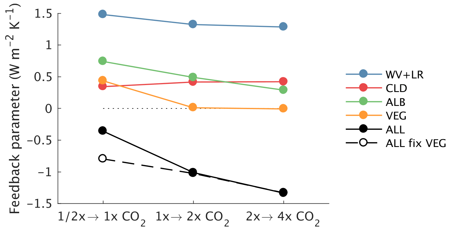
Figure 24 State dependence of global feedback parameters for CLIMBER-X. The feedbacks are for CO₂ doubling starting from different initial CO₂ concentrations (140, 280 and 560 ppm, from left to right). The feedbacks are computed from simulations where vegetation is prescribed at its pre-industrial state. The vegetation feedback is diagnosed from the difference in the sum of all feedbacks between simulations with dynamic and fixed vegetation. The sum of all the feedbacks also includes the contribution from the Planck feedback, which is not shown.

PALADYN has been complemented with a parameterization of dust emissions following the CLIMBER-2 scheme as described in Bauer and Ganopolski (2010). Dust is emitted into the atmosphere from deserts and grasslands whenever the soil is dry enough and the wind speed exceeds a critical threshold.

The snow albedo scheme has been refined with the inclusion of the effect of dust and soot on snow albedo following Dang et al. (2015), and the snow grain size parameterization has been retuned using output of the regional climate model MARv3.6 simulations for Greenland (Fettweis et al., 2017). The parameterization for sub-grid snow cover fraction has been updated with a dependence on the standard deviation of orography following Roesch et al. (2001). More details on the updated surface albedo scheme can be found in Appendix D.

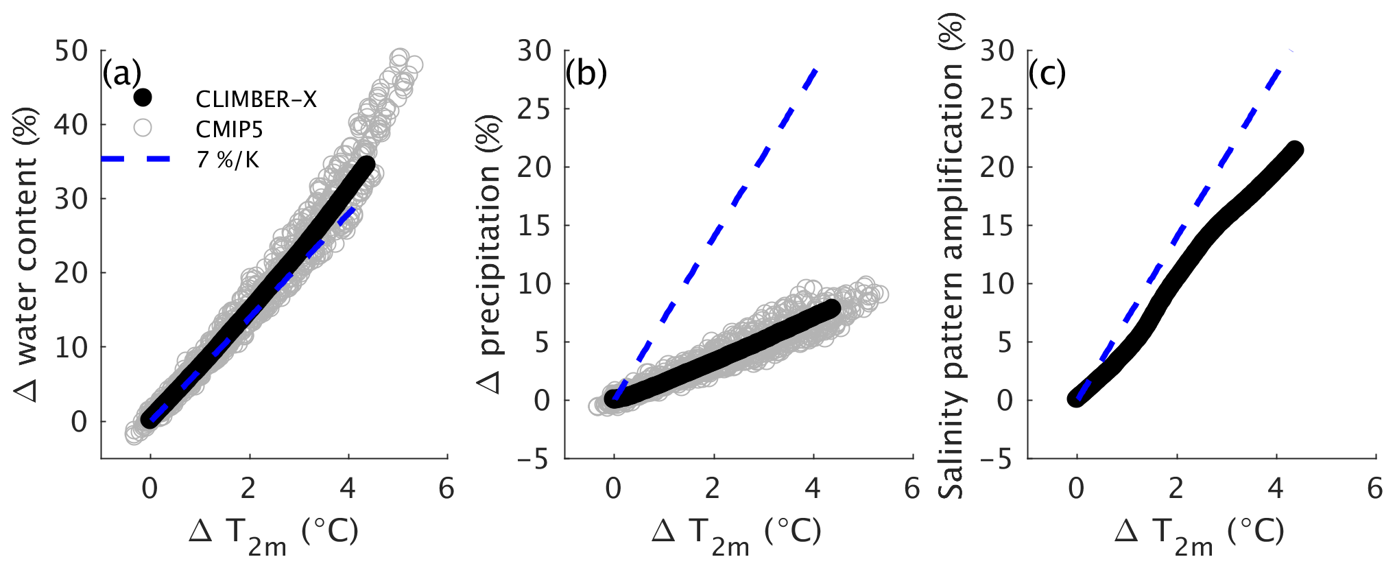
Figure 25 Relative (a) global water content change, (b) global precipitation change and (c) salinity pattern amplification versus global temperature change for the CLIMBER-X and CMIP5 models from the 1 % yr⁻¹ CO₂ increase experiment. Each circle represents 1 year of the simulations.

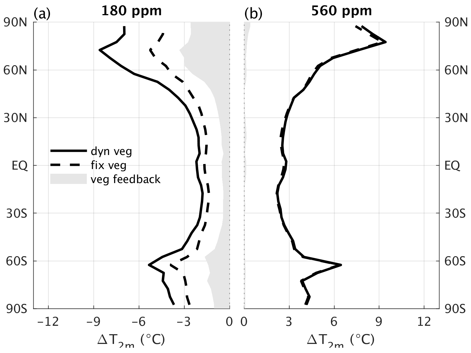
Figure 26 Zonal mean temperature response for atmospheric CO₂ concentrations of (a) 180 ppm and (b) 560 ppm relative to 280 ppm with (solid) and without (dashed) vegetation feedback.

Figure 27 Simulated dominant plant functional types at equilibrium for (a) the pre-industrial control, (b) 180 ppm and (c) 560 ppm of atmospheric CO₂.

CLIMBER-X, and therefore also PALADYN, does not resolve the diurnal cycle. However, diurnal variations can be important, particularly for highly non-linear processes such as snowmelt. For instance, even if the daily mean surface air temperature is below freezing, the daily maximum temperature could still be substantially above the freezing point, thus leading to snowmelt during the day. In the presence of a relatively thin snow layer it is likely that the snow melted during the day would not completely refreeze during the night but would infiltrate into the soil or contribute to surface runoff. Following this line of thought, a parameterization of the diurnal cycle for snowmelt, partly following Krapp et al. (2017), has been implemented to accelerate the spring-time retreat of snow-covered area, which was too slow in the original PALADYN formulation (Willeit and Ganopolski, 2016). The diurnal cycle of skin temperature is assumed to have a sinusoidal shape with the amplitude depending on the difference between daily mean and daily minimum net shortwave radiation at the surface. The latter is computed from the diurnal cycle of insolation at the top of the atmosphere, which is available from the insolation module, using the daily mean surface albedo. If the resulting daily maximum skin temperature is above the freezing point, the energy flux available for snowmelt is computed following Krapp et al. (2017).

The possibility of prescribing land use changes has also been introduced into PALADYN following Burton et al. (2019). A fraction of each grid cell is prescribed as being used for agriculture, with no distinction between cropland and pasture being made. Land use is then represented as a limitation to the space available for a plant functional type (PFT) to expand into. For instance, the three woody PFTs (broadleaf trees, needleleaf trees and shrubs) are prevented from growing in the agricultural fraction, while the two grass PFTs (C₃ grass and C₄ grass) are allowed to grow anywhere in the grid cell and are simply interpreted as agricultural grasses if they grow into the pasture or cropland grid cell fraction. The representation of the effect of land use change on land carbon fluxes will be discussed in more detail in the CLIMBER-X companion paper about the global carbon cycle.

Since the original PALADYN publication, lakes have been introduced as an additional surface type in the model. Lake fractions are prescribed. Lake thermodynamics follows the implementation in CLM4.5 (Oleson et al., 2013; Subin et al., 2012) and includes freezing and melting of lake water and a single snow layer on top of lake ice. Temperatures and ice fractions are simulated for seven vertical layers, with a top-layer thickness of 1 m and the bottom-layer thickness depending on the depth of the lake, which is determined from lake bathymetry. For unfrozen lakes, convective mixing occurs in the lake if the density stratification becomes unstable. Additional vertical mixing occurs when partly frozen layers exist below not fully frozen layers in order to keep ice contiguous at the top of the lake. It is additionally always ensured that the lake is mixed to a minimum depth of 20 m. The surface energy fluxes over lakes are computed similarly to the other surface types as described in Willeit and Ganopolski (2016).

3 Model tuning

Tuning is an essential step in the development of any Earth system model. In such models a number of parameters are uncertain, either because they are poorly constrained by observations or because they are used to describe processes that cannot be explicitly represented in the model (e.g. Mauritsen et al., 2012). These uncertain parameters are then adjusted in such a way as to minimize some measure of the distance between simulated and observed characteristics. In CLIMBER-X some processes that are explicitly represented in state-of-the-art climate models are parameterized instead, introducing some additional parameters that have to be properly calibrated. This refers in particular to the vertical structure of the atmosphere and friction in the ocean.

CLIMBER-X in general has been tuned to present-day climatological fields that are available from observations, reanalysis products and, in some cases, results from state-of-the-art model simulations. Climate feedbacks and model sensitivities have been considered an additional source of information in the process of model calibration, in particular for the parameterization of cloud properties.

The atmosphere model tuning involved a few steps. In the first step the longwave and shortwave radiative transfer schemes have been tuned offline. Shortwave and longwave radiation parameters were tuned in offline mode in order to minimize the root mean square error in top-of-the-atmosphere and surface radiation fluxes. Additional constraints on model parameters are provided by the total greenhouse effect separation presented in Schmidt et al. (2010) and by the radiative kernels of Shell et al. (2008), Block and Mauritsen (2013), Smith et al. (2018) and Pendergrass et al. (2018). More details on the offline tuning of shortwave and longwave radiation are available in Appendices A7 and A8. In the second step, the atmosphere model has been tuned in a coupled model set-up but using sea surface temperature relaxation for the ocean model in order to ensure that sea surface temperatures are close to present-day observations. Tuning parameters in the atmosphere model include parameters describing cloud cover fraction, cloud top height, cloud optical thickness, temperature lapse rate, height of the tropopause, strength of the Hadley and Ferrel cells and macro diffusivities for heat and water.

The land model has been tuned offline forced by prescribed climate variables as described in Willeit and Ganopolski (2016). The tuning of the snow grain size needed in the snow albedo parameterization has been performed offline using results of simulations with the regional climate model MAR for Greenland (Appendix D).

The ocean model tuning has been performed offline using sea surface temperature and sea surface salinity relaxation to observations. Ocean tuning parameters include friction and isopycnal and diapycnal diffusivities.

The sea ice model has been tuned in the fully coupled model set-up. Sea ice model tuning parameters include the thickness of newly formed sea ice, bare sea ice albedo and friction velocity below sea ice.

The coupling between the different model components introduces feedbacks that can substantially alter the performance of the model compared to the various offline or semi-coupled set-ups. A fine-tuning of the fully coupled model is therefore essential and has constituted a substantial part of the CLIMBER-X tuning procedure. The coupled model tuning was performed relying on a largely subjective and heuristic approach, with the goal of primarily minimizing the model–data mismatch in terms of global mean and zonal mean surface air temperature, global mean radiative fluxes at the top of the atmosphere (TOA) and at the surface and seasonal sea ice cover.

In the following we present results of model simulations performed using a single set of model parameters, produced based mainly on subjective ideas about “good” model performance. In the future we are planning to generate an ensemble of model versions selected using more formalized criteria to allow for a quantitative assessment of model uncertainties.

4 Model evaluation for the historical period and present day

The historical period, with its extensive availability of climate data from direct observations, forms the basis for the evaluation of any climate model. Here we evaluate the performance of CLIMBER-X for the climatological period from 1981 to 2010 and for the period of time from 1850 to 2015, corresponding to the historical period covered by CMIP (Coupled Model Intercomparison Project) simulations. For that we compare the results of CLIMBER-X simulations to different observation-based datasets as well as atmosphere and ocean reanalysis data. To give an overview of how CLIMBER-X compares to state-of-the-art general circulation models, we also include results from model simulations from the recent coupled model intercomparison projects. CMIP5 (Taylor et al., 2012) and CMIP6 (Eyring et al., 2016) model data are used interchangeably according to data availability.

The forcings for the historical CLIMBER-X simulations include variations in solar radiation (Matthes et al., 2017), radiative forcing of volcanic eruptions (IPCC, 2013), globally uniform CO₂, CH₄ and N₂O concentrations from Köhler et al. (2017), globally uniform CFC11 and CFC12 concentrations from Meinshausen et al. (2017), and 3-D O₃ concentrations and 2-D SO₄ load from the ensemble mean of CMIP6 models and land use change (pasture and cropland fractions) from Ma et al. (2020). The model is initialized from a 5000-year equilibrium simulation with pre-industrial boundary conditions.

4.1 1981–2010 climatology

In the following, different simulated climatological characteristics are compared to observations to assess the model performance for the present day. Unless stated otherwise, the comparison to observations is for the time interval from 1981 to 2010.

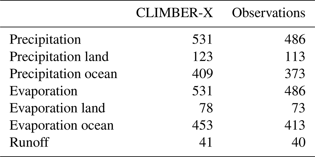
The global mean near-surface air temperature averaged over the time period 1981–2010 in CLIMBER-X is 14.1 ^∘C, which compares well to the 14.35 ^∘C in ERA-Interim reanalysis and is in the middle of the wide range of roughly 13–15 ^∘C spanned by CMIP5/6 models (e.g. Bock et al., 2020). Global temperature is largely determined by the global radiation and energy budget, whose components are in good agreement with observations and CMIP5 models, as shown in detail in Table 1. The strength of the hydrological cycle is a bit overestimated in the model, resulting in higher evaporation and precipitation than observed, particularly over the ocean (Table 2). Note that, while the global latent heat flux in CLIMBER-X is underestimated compared to the observations in Table 1, the global evaporation is overestimated relative to the observational estimates in Table 2. This is a result of the use of different observation-based estimates for the energy fluxes and for the hydrological cycle and is thus ultimately a consequence of the uncertainty in these estimates.

Table 1 Earth's radiation and energy budget in CLIMBER-X compared to observations and CMIP5 models from Wild et al. (2013). The unit is W m⁻².

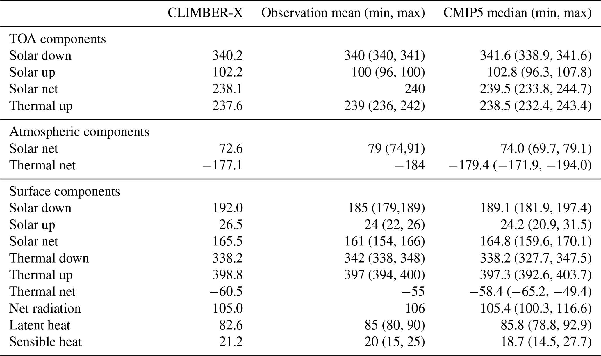
Table 2 Global hydrological cycle in CLIMBER-X compared to observations (Trenberth et al., 2007). The unit is 10¹⁵ kg yr⁻¹.

Atmosphere and ocean dynamics play an important role in the climate system by transferring energy from low to high latitudes, thereby reducing the Equator-to-pole temperature gradient arising from differential solar heating. The total meridional energy transport simulated by CLIMBER-X is compared to observation-based estimates in Fig. 2a. Overall the agreement is good, with a slight underestimate of the peak poleward energy transport. The meridional energy transport by the atmosphere, which constitutes the dominant contribution to total energy transport, matches well with observations (Fig. 2b). A separation of the different atmospheric processes contributing to latitudinal energy transport is also shown in Fig. 2b, including the partition between dry static energy and latent heat fluxes and the contribution by eddies. Eddies dominate the meridional energy transport at mid to high latitudes, while the Hadley cells are the most important contribution in the tropics, in agreement with a similar decomposition performed with other models (e.g. Yang et al., 2015).

The mean meridional circulation in the atmosphere is characterized by the presence of six cells and is a defining feature of atmospheric dynamics. Figure 3 shows that the parameterization of the meridional circulation employed in CLIMBER-X does a reasonable job at describing the Hadley cells in the tropics and the Ferrel cells at mid latitudes.

The zonal mean SLP, which is directly related to the mean meridional circulation, shows good agreement with reanalysis data for both December–February (DJF) and June–August (JJA) (Fig. 4c, f). The model also reproduces the main features of observed azonal SLP, such as the highs over land and lows over the ocean in Northern Hemisphere winter (Fig. 4a, b) and vice versa during summer (Fig. 4d, e).

The simulated near-surface air temperature is compared to reanalysis in Fig. 5. In the zonal mean, the simulated temperatures fall mostly within the range given by different CMIP6 models (Fig. 5c, g). The main model biases include too warm temperatures over eastern continents in NH winter, too cold tropics, particularly over land, and a warm bias over East Antarctica (Fig. 5b, f). The absolute model bias is generally comparable to the bias seen in CMIP6 models, except for the tropics (Fig. 5d, h). The cold bias in the tropics is not only a surface feature, but is also persistent throughout the troposphere (Fig. 6). The rest of the 3-D temperature structure is well simulated by the model, indicating that the vertical variations in temperature can be reasonably well-described by the employed lapse rate parameterization. Zonal mean temperature biases are below a few degrees over large parts of the domain. During the winter months, CLIMBER-X also captures the near-surface temperature inversions at high latitudes. The simulated tropopause height shows a realistic latitudinal profile but is generally a few kilometres too low in the tropics (Fig. 6). CLIMBER-X also reproduces the higher seasonal variations in temperature over the continents compared to the ocean, in particular at high latitudes (Fig. 7).

The simulated atmospheric relative humidity is generally high in the planetary boundary layer and shows pronounced minima in the subtropics, broadly in agreement with observations (Fig. 8). The model does a reasonably good job at reproducing the observed precipitation distribution (Fig. 9). In terms of zonal mean precipitation, the peak associated with the intertropical convergence zone (ITCZ), the minima in the subtropics and the maxima at mid latitudes are well captured by the model (Fig. 9c, f). The main deficiencies are found in the subtropics, with too much precipitation simulated over the ocean in the subsidence areas (Fig. 9a, b, d, e). This is partly related to the too weak subtropical high-pressure systems (Fig. 4).

Cloud cover in CLIMBER-X shows the characteristic latitudinal profile, with minima in the subtropical subsidence areas and maxima in the tropics and at mid to high latitudes (Fig. 10a, f). A realistic simulation of cloud cover is a prerequisite for a good representation of radiation fluxes. Both shortwave and longwave radiation fluxes at the top of the atmosphere are in good agreement with satellite observations and reanalysis (Fig. 10b, d, g, i). The zonal mean radiative fluxes are generally within the range of CMIP5 models (Fig. 10c, e, h, j). Net shortwave radiation at TOA is slightly overestimated at high latitudes in NH summer (Fig. 10h), while net longwave TOA radiation exhibits some systematic biases in the tropics (Fig. 10e, j).

The ocean overturning circulation in CLIMBER-X is characterized by the presence of an Atlantic overturning cell and by Antarctic bottom water formation (Fig. 11). The maximum of the Atlantic overturning streamfunction at 26^∘ N is 18.5 Sv, a bit higher than indicated by observations (Frajka-Williams et al., 2021) (Fig. 12). The simulated Atlantic meridional circulation (AMOC) penetration depth of ∼ 3800 m, as measured by the zero crossing in the streamfunction, is about 500 m too shallow compared to that directly observed, a problem common also to many CMIP6 models (Fig. 12). The maximum meridional heat transport by the Atlantic Ocean is ∼ 1.12 PW, slightly lower than observation-based estimates of ∼ 1.25 PW (e.g. Johns et al., 2011). The discrepancy between stronger-than-observed AMOC and the weaker-than-observed Atlantic meridional heat transport can be explained by biases in the simulated vertical structure of the transport (Fig. 12) and in the Atlantic Ocean temperature field (Fig.14). Deep water forms in the model at several locations in the northern North Atlantic, i.e. in the Labrador Sea south of Greenland and in the Nordic Seas, in agreement with observational estimates (Fig. 13). Deep water is also formed at several locations around Antarctica, mostly on the continental shelf, as shown by the annual maximum mixed-layer depth in Fig. 13. No deep water is formed in the North Pacific.

Ocean temperature and salinity fields compare well to observations in the deep ocean (Figs. 14, 15), with model biases mostly concentrated in the upper 1000 m. Biases in simulated temperature include too cold intermediate waters in the subtropics in the Atlantic and Indian oceans and too warm surface water in the North Pacific (Fig. 14c, f, i). Salinity biases of up to 1 psu are present in all ocean basins in the upper ∼ 1000 m (Fig. 15c, f, i).

The seasonality in sea ice area in both the NH and Southern Hemisphere (SH) is well reproduced by CLIMBER-X (Fig. 16) and is mostly within the range of CMIP6 models. The spatial extent of minimum and maximum sea ice cover is also in generally good agreement with observations (Fig. 17). Arctic winter sea ice cover is overestimated in the Fram Strait, while it is underestimated in the Sea of Okhotsk (Fig. 17a, e). Minimum and maximum sea ice extents in the Southern Ocean are well represented in the model (Fig. 17b, d, f, h).

The simulated total permafrost area is 18.5×10⁶ km², close to the observed value of 18.8×10⁶ km² (e.g. Tarnocai et al., 2009). In terms of spatial extent, permafrost area is in good agreement with observations over Eurasia, while it is underestimated in eastern Canada (Fig. 18).

4.2 Simulations for the historical period

The CLIMBER-X-simulated historical evolution of global mean temperature is compared to observations (Morice et al., 2012) and CMIP6 models in Fig. 19a. The model reproduces rather well the observed historical temperature trends and the response to volcanic eruptions. CLIMBER-X does not represent internal climate variability, and its results therefore cannot be compared one to one to observations. However, the simulated temperature shows a very good match with the ensemble mean of CMIP6 models, where internal variability has effectively been removed. The contribution of the different forcings to the historical temperature evolution also shows good agreement with the corresponding CMIP6 ensemble means, except for the last 2 decades, when CMIP6 models tend to overestimate the observed temperature change (Fig. 19b–d).

The rate of heat uptake by the ocean is consistent with observations (Levitus et al., 2012) until around the year 2000 but is overestimated after that (Fig. 20). However, the historical ocean heat uptake in CLIMBER-X is in better agreement with observations compared to most EMICs, including CLIMBER-2 (Eby et al., 2013).

5 Model sensitivities

Present-day observations provide a relatively poor constraint on model sensitivities to different climate forcings. Comparison to state-of-the-art general circulation models for experiments with different forcings and boundary conditions is therefore crucial for a model like CLIMBER-X. To this end we performed a comprehensive analysis of climate feedbacks, compared the response to changes in CO₂ for standard CMIP abrupt4xCO2 ​​​​​​​ and 1 % yr⁻¹ CO₂ increase experiments, evaluated the vegetation feedback and tested the response to last glacial maximum boundary conditions, which provides insights into the model response to different orbital configurations, topographies and land–sea masks. We also performed standard freshwater hosing experiments to investigate the stability properties of the Atlantic meridional ocean circulation. An overview of the results of these experiments is presented next.

5.1 Transient climate response, climate sensitivity and Charney feedbacks

The equilibrium climate sensitivity of the standard version of CLIMBER-X is 3.3 K as computed from the temperature change at equilibrium (5000-year-long experiment) for a doubling of atmospheric CO₂. This is in the middle of the range of 1.5–4.5 initially derived by Charney et al. (1979), which is also the estimated range given by the latest IPCC report (IPCC, 2021). The transient climate response of CLIMBER-X, defined as the global temperature change at the time of CO₂ doubling in 1 % yr⁻¹ CO₂ increase experiments, is 1.9 K. A plot of equilibrium climate sensitivity versus transient climate response shows that CLIMBER-X is also well within the range of CMIP6 models (Fig. 21).

CLIMBER-X includes code to diagnose the strength of the different climate feedbacks, which allows for a more detailed analysis of the processes controlling climate sensitivity in the model. The feedbacks are evaluated using the partial radiation perturbation method (Bony et al., 2006; Wetherald and Manabe, 1988). In this method, partial derivatives of model top-of-the-atmosphere radiation with respect to changes in modelled fields (such as water vapour, lapse rate and clouds) are determined by diagnostically rerunning the model radiation code.

The global feedback parameters for CLIMBER-X computed for CO₂ doubling relative to 280 ppm are shown in Fig. 22 and generally compare well to feedback parameters computed for different models (e.g. Bony et al., 2006). The water vapour feedback is the largest positive feedback in the model, followed by cloud and albedo feedbacks. The lapse rate feedback is globally negative, in agreement with CMIP5 models (Fig. 22).

A look at the zonal mean feedback parameters gives further insight into the spatial distribution of the feedbacks (Fig. 23). The albedo feedback is large at high latitudes and is related to the sea ice retreat and reduced snow cover in a warmer climate (Fig. 23e). The water vapour feedback is associated with an increase in water vapour content in a warmer atmosphere and is larger in the tropics than at the poles (Fig. 23f). The lapse rate feedback is negative in the tropics because of the larger warming of the mid–upper troposphere relative to the surface, while it is large and positive at high latitudes as a result of a pronounced erosion of surface temperature inversions mainly due to retreating sea ice (Fig. 23g). These results are all in agreement with feedbacks diagnosed in different general circulation models (e.g. Colman et al., 2001; Crook et al., 2011). Feedbacks related to clouds are the most uncertain and account for a large portion of the spread in climate sensitivity within current general circulation models (e.g. Zelinka et al., 2020). Clouds affect both longwave and shortwave radiation at the top of the atmosphere through different processes. Cloud feedbacks in CLIMBER-X are shown in Fig. 23b–d, including a separation into contributions from changes in cloud fraction, cloud optical thickness and cloud height. The net cloud feedback is positive at all latitudes, with the notable exception of the Southern Ocean, where a pronounced increase in optical thickness with warming causes a large negative shortwave cloud feedback. Shortwave and longwave radiation cloud feedbacks generally act to (at least partly) compensate in CLIMBER-X (Fig. 23c–d), in agreement with ESMs (e.g. Zelinka et al., 2012). The effects of cloud optical depth changes are generally larger in the shortwave, while changes in cloud height have a larger effect on longwave radiation. Combined, all feedbacks are mostly negative, except at high latitudes, where sea ice melting leads to large positive albedo and lapse rate feedbacks (Fig. 23h).

Climate feedbacks can be state-dependent. This is explored in CLIMBER-X by repeating the feedback analysis for a CO₂ doubling but starting from different baseline CO₂ concentrations, i.e. 140 and 560 ppm, in addition to the standard feedback analysis shown above, which was performed starting from a pre-industrial CO₂ of 280 ppm. The albedo feedback shows a pronounced state dependence in CLIMBER-X, as shown in Fig. 24. In particular, the albedo feedback strongly increases in colder climates due to extended snow and sea ice cover. This is in agreement with previous studies, e.g. Colman and McAvaney (2009). The cloud feedback increases slightly with global temperature, while the sum of water vapour and lapse rate feedbacks decreases as climate warms.

Hydrological sensitivity, which quantifies the relative global precipitation change per unit change in global temperature, is an important measure of the response of the hydrological cycle to climate change (e.g. Held and Soden, 2006). In agreement with CMIP models, CLIMBER-X shows an increase in global precipitation by ∼ 2 % per degree global temperature increase in the 1 %-per-year CO₂ increase experiment (Fig. 25b), while the atmospheric water content increase approximately follows the Clausius–Clapeyron increase of 7 % K⁻¹ (Fig. 25a). It has also been observed that the sea surface salinity pattern is amplified under global warming, with salinity increasing in high-salinity regions and decreasing in low-salinity regions due to an intensification of existing patterns of precipitation–evaporation (e.g. Durack et al., 2012). The salinity pattern amplification (as defined by e.g. Durack et al., 2012) in the 1 %-per-year CO₂ increase simulation in CLIMBER-X is ∼ 5 % per degree global warming (Fig. 25c), in good agreement with estimates from Zika et al. (2018) for the historical period. The salinity pattern amplification is therefore larger than the hydrological sensitivity of the model, possibly due to the effect of ocean warming on surface salinity (Zika et al., 2018).

5.2 Vegetation feedback

Changes in vegetation structure and its spatial distribution can affect the climate through the effect on surface energy and water fluxes (e.g. Levis et al., 1999; Bala et al., 2006; Falloon et al., 2012). In CLIMBER-X, the vegetation feedback amplifies temperature change by more than 1 ^∘C at mid to high northern latitudes for a reduction of CO₂ to 180 ppm (Fig. 26a), while it is small for CO₂ doubling (Fig. 26b). A similar asymmetry in the vegetation feedback between low and high CO₂ has also been found in CLIMBER-2 (Willeit et al., 2014). The reason for the strong positive vegetation feedback for low CO₂ originates from a pronounced southward retreat of boreal forest (Fig. 27b), which causes a substantial increase in surface albedo through the missing snow-masking effect of trees (e.g. Bonan, 2008). In CLIMBER-X, a CO₂ increase leads in general to an expansion of forests and a reduction in desert area, while the opposite happens for lower CO₂ levels (Fig. 27). The strong state dependence of the vegetation feedback can also be seen in Fig. 24, with a very strong feedback for a CO₂ concentration of 140 ppm and negligible vegetation feedback for climates warmer than the present day.

5.3 Last glacial maximum

For the last glacial maximum (LGM), we prescribe boundary conditions following the PMIP4 protocol (Kageyama et al., 2017), with the GLAC-1D ice sheet, bathymetry and land–sea mask reconstruction (Tarasov et al., 2012). The simulation is started from the present-day equilibrium followed by a switch to LGM boundary conditions during which the topography, bathymetry and ocean volume are adjusted. Total ocean salinity is conserved in this process. The model is then run for 5000 years to ensure equilibrium is reached.

The simulated global cooling at the LGM relative to the pre-industrial is 6.2 K, similar to the cooling produced by CLIMBER-2 (Ganopolski et al., 1998). This matches the most recent reconstruction-based estimate by Tierney et al. (2020); however, it is on the cold side of range produced by PMIP4 models (3.3–7.2 K) (Kageyama et al., 2021). The vegetation feedback in the model is responsible for ∼ 0.5 K of the simulated cooling. The zonal mean annual temperature change is compared to PMIP3/4 models in Fig. 28. CLIMBER-X shows a cooling in the tropics that is more pronounced than in most other models, while at high latitudes the temperature difference falls well inside the PMIP3/4 range. In terms of sea surface temperatures, the model results agree well with the proxy-based reconstruction by Tierney et al. (2020) (Fig. 29), which also shows a pronounced cooling in the tropics as opposed to e.g. Paul et al. (2021) (Fig. 29c).

Figure 28 Last glacial maximum annual mean zonal near-surface air temperature differences relative to pre-industrial compared to PMIP3/4 models (Kageyama et al., 2021).

Figure 29 Last glacial maximum annual mean sea surface temperature differences relative to pre-industrial compared to reconstructions (Paul et al., 2021; Tierney et al., 2020).

The global ocean cools by 2.4 ^∘C, in good agreement with 2.57 ± 0.24 ^∘C in Bereiter et al. (2018), with the deep ocean temperature being close to the freezing point of seawater ($<-\mathrm{1}$ ^∘C) in all ocean basins, in accordance with Adkins et al. (2002). The AMOC is weaker and shallower at the LGM relative to the pre-industrial, with a maximum overturning strength of ∼ 14 Sv at 26^∘ N and extending down to a depth of ∼ 2500 m (Fig. 30a). This is contrary to most PMIP3/4 models, which tend to produce a more vigorous and deeper Atlantic overturning at the LGM (Weber et al., 2007; Kageyama et al., 2021) but is possibly in better agreement with proxy reconstructions (e.g. McManus et al., 2004; Bohm et al., 2015). The AMOC weakening is accompanied by a strengthening of Antarctic bottom water formation (Fig. 30b), which is related to an increase in brine rejection associated with a pronounced expansion of sea ice in the Southern Ocean (Fig. 31b), similarly to what has been found in other models (e.g. Nadeau et al., 2019; Shin et al., 2003; Stouffer and Manabe, 2003). The large simulated sea ice expansion in the Southern Ocean is also largely consistent with the latest proxy reconstructions by Lhardy et al. (2021) (Fig. 31b).

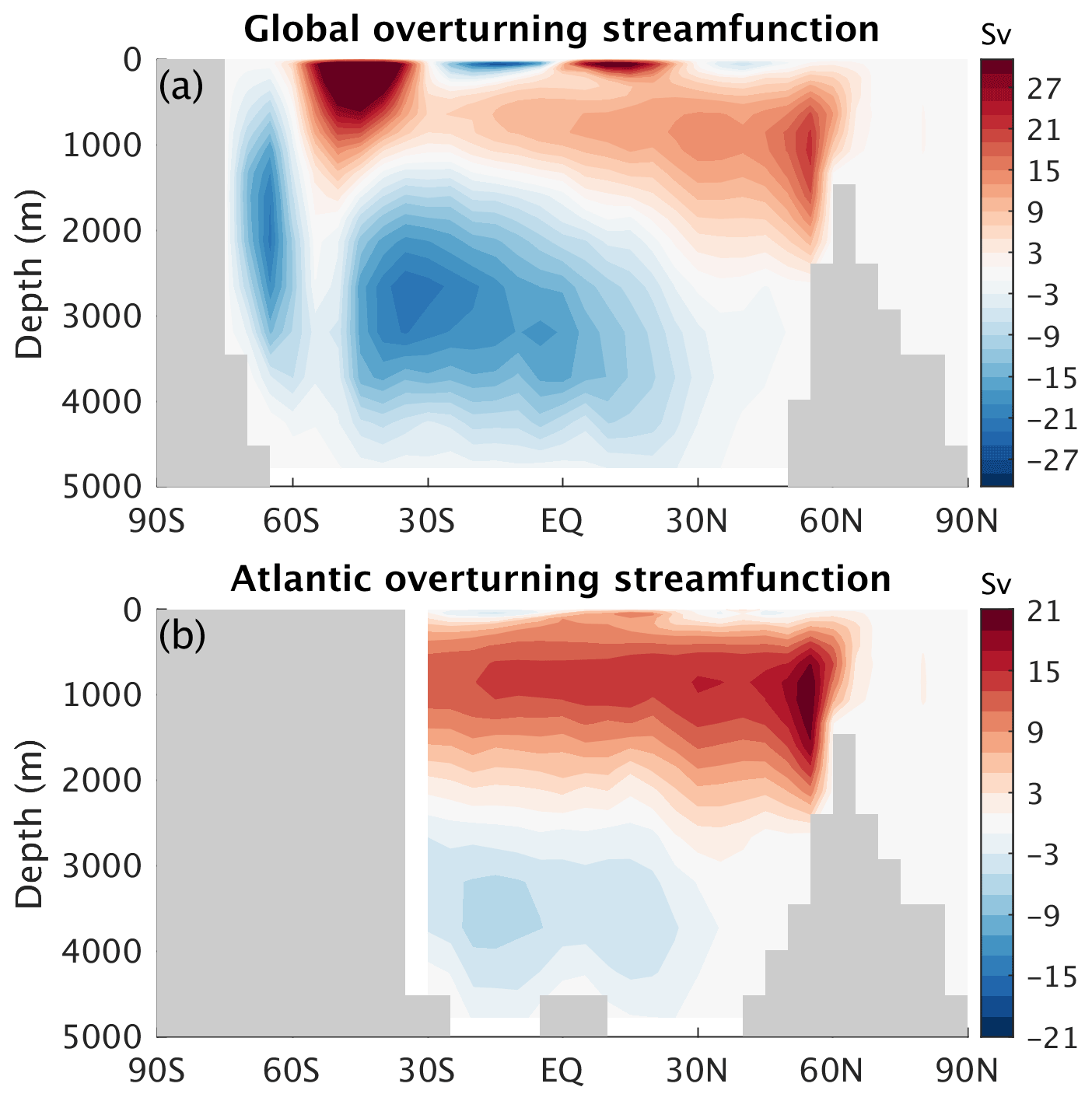
Figure 30 Ocean overturning circulation at the last glacial maximum: (a) global and (b) Atlantic.

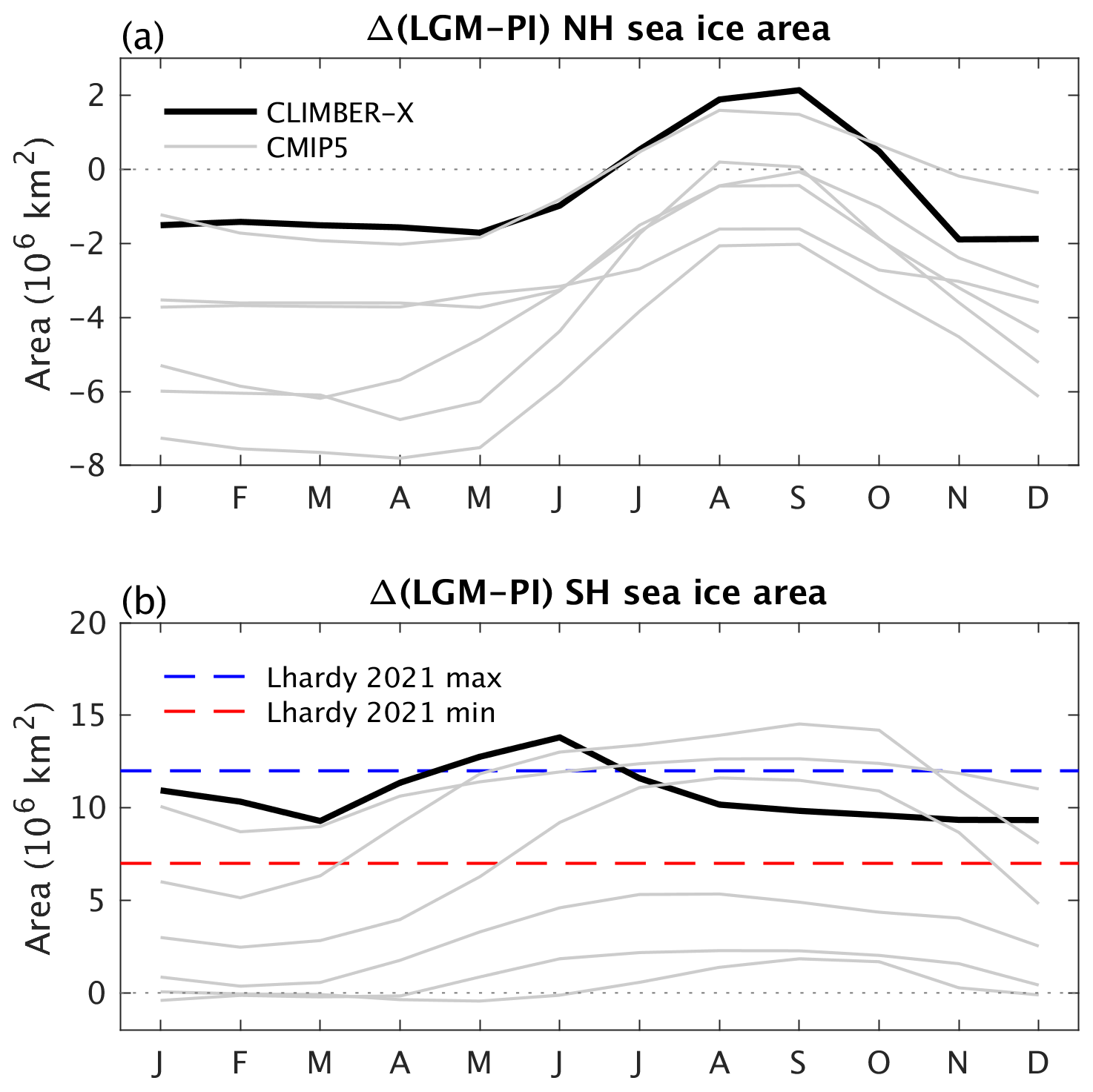
Figure 31 Difference in seasonal sea ice area in the (a) NH and (b) SH between the last glacial maximum and the pre-industrial. CLIMBER-X results (black) are compared to CMIP5 models (grey). In panel (b) the seasonal minimum and maximum changes in SH sea ice area from proxy estimates of Lhardy et al. (2021) are also indicated.

5.4 AMOC stability

The meridional overturning circulation in the Atlantic Ocean plays an important role in the global climate system. Since the pioneering work of Stommel (1961), who used a simple box model to show that the AMOC could have multiple stable states, the stability of the AMOC has received considerable attention, with several studies using ocean general circulation models confirming the bi-stable nature of the system (e.g. Manabe and Stouffer, 1988; Rahmstorf, 1995).

Consistent with findings by other EMICs (Rahmstorf et al., 2005) and low-resolution atmosphere–ocean GCMs (Hawkins et al., 2011), CLIMBER-X also shows a hysteresis behaviour of the AMOC when the freshwater balance of the North Atlantic is perturbed (Fig. 32). The width of the hysteresis for a rate of change of 0.05 Sv kyr⁻¹, which was also used by Rahmstorf et al. (2005), is ∼ 0.25 Sv. However, when quasi-equilibrium simulations (5000 years long) are performed with the model starting from AMOC on and off states for a given constant freshwater hosing flux, the width of the hysteresis is reduced by about a factor of 2 (Fig. 32). This indicates that a rate of change of 0.05 Sv kyr⁻¹ is too high to allow a precise tracking of the actual AMOC stability diagram. Under pre-industrial conditions, the AMOC is in a mono-stable regime in the model although relatively close to the bi-stable regime. The present-day stability of the AMOC is still debated (e.g. Weijer et al., 2019).

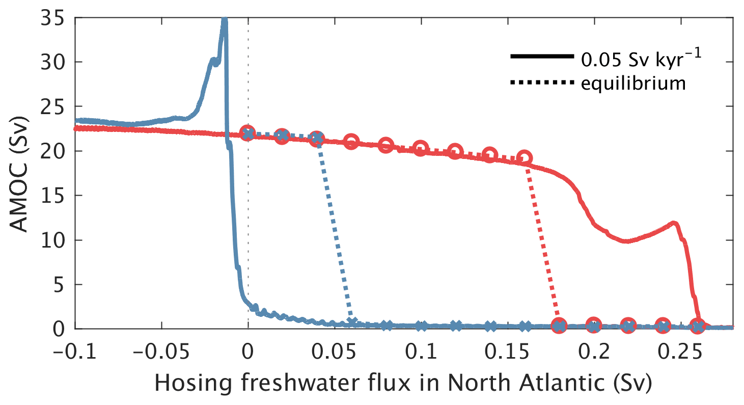
Figure 32 AMOC hysteresis for freshwater hosing applied to the latitudinal belt between 20 and 50 ^∘ N in the Atlantic. The hysteresis curve for experiments where the freshwater hosing is changed at a rate of 0.05 Sv per 1000 years is shown by the solid lines. The symbols and the connecting dotted lines indicate the AMOC strength for quasi-equilibrium simulations with a prescribed constant freshwater hosing rate initialized from an AMOC on state (red circles) and from an AMOC off state (blue crosses).

The different climatic conditions associated with the two equilibrium states of the AMOC are illustrated by mean annual surface air temperature and precipitation differences in Fig. 33. The temperature difference shows the classic seesaw pattern, with cooling in the NH and warming in the SH as a response to AMOC shutdown (Fig. 33a). The cooling reaches up to 10 K in the North Atlantic and is compensated by a warming of up to 10 K in the Southern Ocean. The cooling produced in the North Atlantic is consistent with GCM simulations (e.g. Vellinga and Wood, 2002; Jackson et al., 2015; Pedro et al., 2018), while the large warming in the Southern Ocean is not seen in these GCMs, possibly because they are not run into equilibrium. Precipitation changes in the AMOC off state compared to the on state are clearly seen in the tropics as a result of a pronounced southward shift in the intertropical convergence zone (Fig. 33b). Precipitation is also reduced in the North Atlantic, simply as a consequence of the colder climatic conditions.

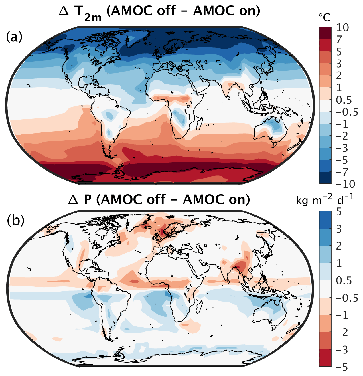
Figure 33 Annual mean (a) near-surface air temperature and (b) precipitation differences between AMOC off and on states.

6 Applicability and limitations of CLIMBER-X

CLIMBER-X does not resolve synoptic variability and does not exhibit interannual internal variability and is therefore not suited to investigating weather extremes or internal climate oscillations like ENSO. The atmospheric component of CLIMBER-X is based on a statistical–dynamical approach, which employs a number of significant simplifications and assumptions. Such an approach allows us to develop a model that is several orders of magnitude faster than GCMs with similar resolution; however, these simplifications and a set of parameterizations explicitly derived from present-day climate limit the model's applicability to climate states fundamentally different from the present.

7 Conclusions

We have described the major features of the climate component of the newly developed CLIMBER-X Earth system model. CLIMBER-X relies on the geostrophic approximation for the description of both atmospheric and oceanic circulation. It does not explicitly resolve atmospheric and oceanic eddies, but the effect of both is parameterized as a diffusive process. The simplified dynamics, together with the use of a daily time step for most processes and the lower spatial resolution of $\mathrm{5}{}^{\circ }\times \mathrm{5}{}^{\circ }$, provides a substantial advantage in terms of computational costs relative to general circulation models, which are based on the primitive equations. Nevertheless, in terms of the number of physical processes which are represented in the model, CLIMBER-X is comparable to state-of-the-art climate models. This is highlighted for instance by the realistic representation of climate feedbacks in the model. Moreover, CLIMBER-X also includes a model for the global carbon cycle and is coupled to an ice sheet model (both of which will be described in detail in forthcoming papers) and thus allows simulations of the evolution of the Earth system as a whole and the investigation of complex interactions and feedbacks between different components of the Earth system on timescales ranging from decades to hundreds of thousands of years. CLIMBER-X is therefore an ideal tool to explore the long-term past and future evolution of the Earth system.

Appendix A: SESAM detailed description

A1 Vertical structure

SESAM is based on a number of simplifications compared to current state-of-the-art atmospheric models. One such simplification is that, in all equations apart from that describing atmospheric dynamics, the atmospheric pressure at each model level is not computed using the hydrostatic approximation but is assumed to be an exponential function of the height above sea level only:

$$\begin{array}{}\text{(A1)}& p\left(z\right)=p_{\mathrm{0}}{e}^{-\frac{z}{H_{\mathrm{a}}}},\end{array}$$

where $H_{\mathrm{a}}=R_{\mathrm{d}}{T}_{\mathrm{0}}/g$ is the atmospheric height scale. The mean sea-level pressure p₀ is determined from the atmospheric mass conservation condition:

$$\begin{array}{}\text{(A2)}& \underset{\mathrm{\Omega }}{\int }p\left(z_{\mathrm{s}}\right)\mathrm{d}\mathit{\omega }={\displaystyle \frac{M_{\mathrm{a}}g}{A_{\mathrm{e}}}},\end{array}$$

where Ω indicates the surface of the Earth, z_s is surface elevation above sea level, M_a is the total atmospheric mass and A_e is the area of the Earth's surface. Hence, the mean sea-level pressure will change with changing topography.

For atmospheric dynamics the dependence of pressure on atmospheric temperature is explicitly accounted for through the parameterization of sea-level pressure and through the thermal wind equation (see Appendix A2 below).

Air density is described as a function of elevation:

$$\begin{array}{}\text{(A3)}& \mathit{\rho }\left(z\right)={\mathit{\rho }}_{\mathrm{0}}{e}^{-\frac{z}{H_{\mathrm{a}}}},\end{array}$$

with the reference density at sea level computed from the ideal gas law:

$$\begin{array}{}\text{(A4)}& {\mathit{\rho }}_{\mathrm{0}}={\displaystyle \frac{p_{\mathrm{0}}}{R_{\mathrm{d}}{T}_{\mathrm{0}}}}.\end{array}$$

The vertical profile of temperature is computed as follows:

$$\begin{array}{}\text{(A5)}& T\left(z\right)=T_{\mathrm{a}}-\underset{z_{\mathrm{s}}}{\overset{z}{\int }}\mathrm{\Gamma }\left(z^{\prime }\right)\mathrm{d}{z}^{\prime },\end{array}$$

where T_a is the prognostic atmospheric temperature at the surface and Γ is the lapse rate. Although the atmospheric temperature lapse rate is remarkably close to a constant value of ∼ 6.5 K km⁻¹, the deviations from this value are important in order to reproduce both a realistic present-day climate and climate feedbacks. In SESAM, Γ is parameterized as

$$\begin{array}{}\text{(A6)}& \mathrm{\Gamma }\left(z\right)=\left\{\begin{array}{l}{\mathrm{\Gamma }}_{\mathrm{s}},z\le z_{\mathrm{s}}+H_{\mathrm{\Gamma },\mathrm{s}},\\ {\mathrm{\Gamma }}_{\mathrm{b}}+\left({\mathrm{\Gamma }}_{\mathrm{t}}-{\mathrm{\Gamma }}_{\mathrm{b}}\right)\frac{z}{H_{\mathrm{\Gamma },\mathrm{t}}},z>z_{\mathrm{s}}+H_{\mathrm{\Gamma },\mathrm{s}}\\ \text{and}z\le H_{\mathrm{T}},\\ \mathrm{0},z>H_{\mathrm{T}}.\end{array}\right.\end{array}$$

In general, the lapse rate therefore linearly increases with height, with Γ_b and Γ_t depending on atmospheric humidity q_a only:

$$\begin{array}{}\text{(A7)}& {\displaystyle }& {\displaystyle }{\mathrm{\Gamma }}_{\mathrm{b}}=c_{\mathrm{1}}^{\mathrm{\Gamma }}-c_{\mathrm{2}}^{\mathrm{\Gamma }}{q}_{\mathrm{a}},\text{(A8)}& {\displaystyle }& {\displaystyle }{\mathrm{\Gamma }}_{\mathrm{t}}={\mathrm{\Gamma }}_{\mathrm{b}}-c_{\mathrm{2}}^{\mathrm{\Gamma }}{q}_{\mathrm{a}}+c_{\mathrm{3}}^{\mathrm{\Gamma }}.\end{array}$$

In a layer close to the surface, the lapse rate depends on near-surface stability:

$$\begin{array}{}\text{(A9)}& {\mathrm{\Gamma }}_{\mathrm{s}}=\left\{\begin{array}{l}{c}_{\mathrm{4}}^{\mathrm{\Gamma }}\sqrt{max\left(\mathrm{0},T_{\mathrm{a}}-T_{\star }\right)},\text{ocean},\\ c_{\mathrm{5}}^{\mathrm{\Gamma }}\left(T_{\mathrm{a}}-T_{\star }\right),\text{land and}{T}_{\mathrm{a}}-T_{\star }>\mathrm{0},\\ c_{\mathrm{6}}^{\mathrm{\Gamma }}\left(T_{\mathrm{a}}-T_{\star }\right),\text{land and}{T}_{\mathrm{a}}-T_{\star }<\mathrm{0},\\ c_{\mathrm{5}}^{\mathrm{\Gamma }}\left(T_{\mathrm{a}}-T_{\star }\right),\text{ice},\end{array}\right.\end{array}$$

where T_⋆ is the skin temperature and Γ_s is limited to be lower than $\mathrm{7.5}\times {\mathrm{10}}^{-\mathrm{3}}$ K m⁻¹ over ocean and $\mathrm{10}\times {\mathrm{10}}^{-\mathrm{3}}$ K m⁻¹ over land and ice. In particular, Eq. (A9) allows SESAM to reproduce near-surface inversions which are important for surface climate.

The tropopause height H_T is derived assuming that the stratosphere is in radiative equilibrium:

$$\begin{array}{}\text{(A10)}& {\displaystyle \frac{\partial H_{\mathrm{T}}}{\partial t}}=-c_{\mathrm{1}}^{\mathrm{tp}}\left(R_{\mathrm{str},\mathrm{net}}+S\right).\end{array}$$

The net radiation in the stratosphere, R_str,net, includes the balance of longwave radiation and the shortwave radiation absorbed by ozone. The effect of atmospheric dynamics on tropopause height is explicitly included in the prescribed latitudinal profile of S, which only depends on the position (ϕ_ITCZ) and width (Δϕ_Had) of the Hadley cells:

$$\begin{array}{}\text{(A11)}& S=c_{\mathrm{2}}^{\mathrm{tp}}\left[\mathrm{1}-c_{\mathrm{3}}^{\mathrm{tp}}\left(\mathrm{1}-{\sin }^{\mathrm{8}}{\displaystyle \frac{\mathrm{0.85}\left(\mathit{\varphi }-{\mathit{\varphi }}_{\mathrm{ITCZ}}\right)}{\mathrm{0.5}\mathrm{\Delta }{\mathit{\varphi }}_{\mathrm{Had}}}}\right)\right].\end{array}$$

Potential temperature, which is a conserved quantity for adiabatic motions, is computed as

$$\begin{array}{}\text{(A12)}& \mathit{\theta }\left(z\right)=T\left(z\right)+{\mathrm{\Gamma }}_{\mathrm{d}}z,\end{array}$$

where ${\mathrm{\Gamma }}_{\mathrm{d}}=g/c_{\mathrm{p}}$ is the dry adiabatic lapse rate and c_p is the specific heat capacity of air at constant pressure.

In CLIMBER-2 specific humidity was specified as decaying exponentially with height, but this can imply unrealistic relative humidities in the upper troposphere, where humidity is important for longwave radiation. This problem is also highlighted by the fact that there is no tight coupling between water vapour and lapse rate feedbacks in CLIMBER-2, contrary to what is observed in most climate models. To overcome this limitation, in SESAM the vertical profile of specific humidity is expressed through temperature and a parameterization of the relative humidity variation with height:

$$\begin{array}{}\text{(A13)}& r\left(z\right)=\left\{\begin{array}{ll}{r}_{\mathrm{a}}& z\le z_{\mathrm{pbl}},\\ r_{\mathrm{a}}{e}^{-\frac{z-z_{\mathrm{pbl}}}{H_{\mathrm{r}}}}& z>z_{\mathrm{pbl}}\text{and}z\le z_{\mathrm{s}}+c_{\mathrm{4}}^{\mathrm{r}},\\ r_{\mathrm{a}}{e}^{-\frac{z_{\mathrm{s}}+c_{\mathrm{4}}^{\mathrm{r}}-z_{\mathrm{pbl}}}{H_{\mathrm{r}}}}& z>z_{\mathrm{s}}+c_{\mathrm{4}}^{\mathrm{r}}\text{and}z\le H_{\mathrm{T}},\\ r_{\mathrm{st}}& z>H_{\mathrm{T}},\end{array}\right.\end{array}$$

where $z_{\mathrm{pbl}}=z_{\mathrm{s}}+c_{\mathrm{5}}^{\mathrm{r}}$ is the elevation of the planetary boundary layer. The relative humidity height scale H_r is constant and uniform in the extratropics and depends on vertical velocity at 700 hPa in the tropics:

$$\begin{array}{}\text{(A14)}& H_{\mathrm{r}}=f_{\mathrm{trop}}\cdot c_{\mathrm{1}}^{\mathrm{r}}\cdot e^{c_{\mathrm{2}}^{\mathrm{r}}\cdot w_{\mathrm{700}}}+(\mathrm{1}-f_{\mathrm{trop}})\cdot c_{\mathrm{1}}^{\mathrm{r}}\cdot c_{\mathrm{3}}^{\mathrm{r}},\end{array}$$

with $f_{\mathrm{trop}}=\mathrm{1}-{\sin }^{\mathrm{8}}\mathit{\phi }$, where φ is defined below in Appendix A2. Specific humidity is then computed as

$$\begin{array}{}\text{(A15)}& q\left(z\right)=r\left(z\right)\cdot q_{\mathrm{sat}}\left(T\right(z),p(z\left)\right),\end{array}$$

where the specific humidity at saturation q_sat is computed assuming saturation over ice at temperatures below −15 ^∘C, saturation over water at temperatures above T₀ and a weighted mean of saturation over water and ice in the intermediate temperature range.

Table A1 Parameters for vertical structure.

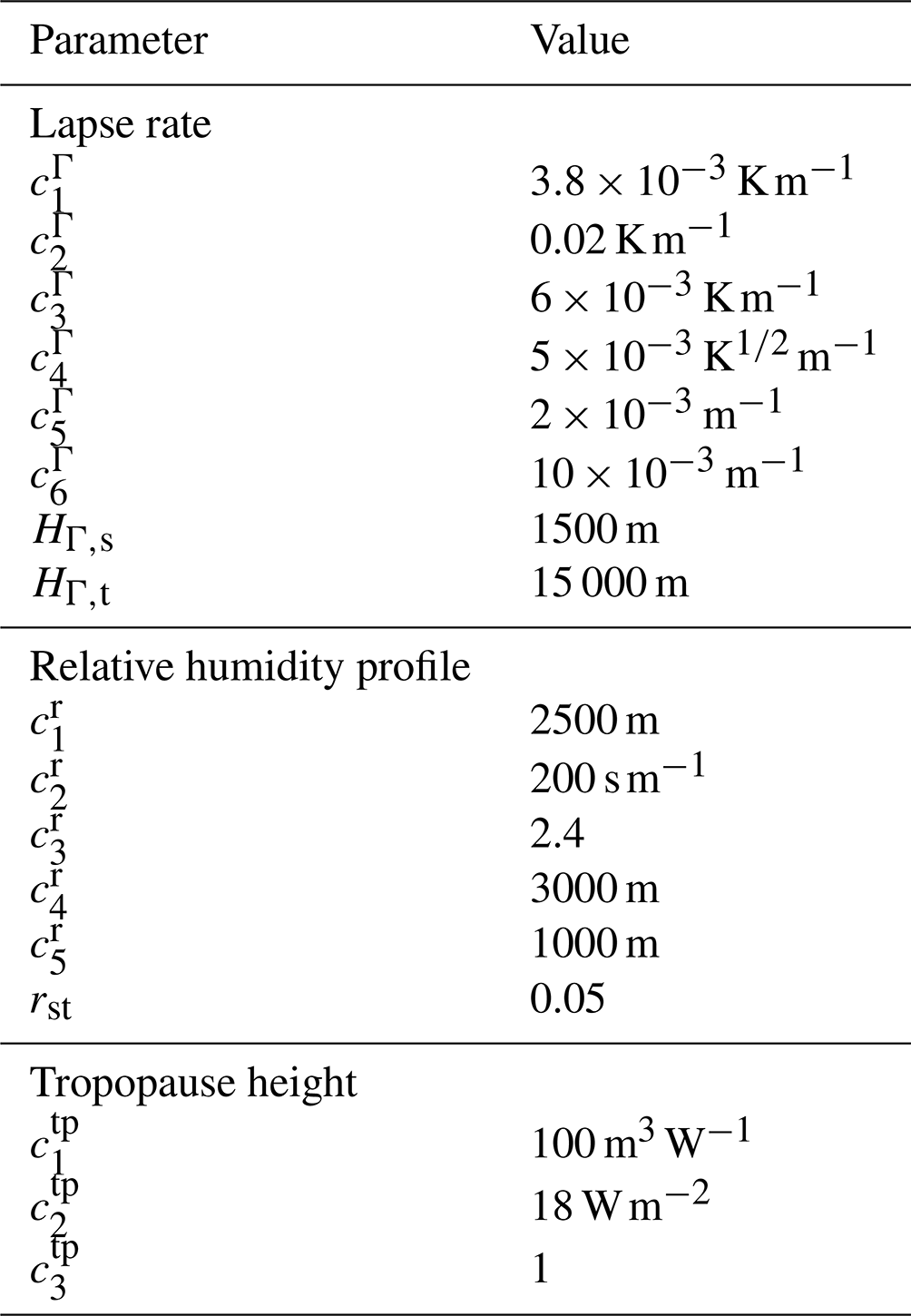
A2 Dynamics

The dynamics of the atmosphere in SESAM is similar to that in CLIMBER-2 but with several notable improvements.

Horizontal velocity in the atmosphere is computed as the sum of geostrophic and ageostrophic components:

$$\begin{array}{}\text{(A16)}& \mathit{u}={\mathit{u}}_{\mathrm{g}}+{\mathit{u}}_{\mathrm{a}}.\end{array}$$

The geostrophic components of velocity at any height within the troposphere are obtained using the thermal wind approximation:

$$\begin{array}{}\text{(A17)}& {\displaystyle }& {\displaystyle }{u}_{\mathrm{g}}\left(z\right)=-{\displaystyle \frac{\mathrm{1}}{{\mathit{\rho }}_{\mathrm{0}}f{R}_{\mathrm{e}}}}{\displaystyle \frac{\partial p_{\mathrm{sl}}}{\partial \mathit{\varphi }}}-\underset{\mathrm{0}}{\overset{z}{\int }}{\displaystyle \frac{g}{T_{\mathrm{0}}f{R}_{\mathrm{e}}}}{\displaystyle \frac{\partial T}{\partial \mathit{\varphi }}}\mathrm{d}z,\text{(A18)}& {\displaystyle }& {\displaystyle }{v}_{\mathrm{g}}\left(z\right)={\displaystyle \frac{\mathrm{1}}{{\mathit{\rho }}_{\mathrm{0}}f{R}_{\mathrm{e}}\cos \mathit{\varphi }}}{\displaystyle \frac{\partial p_{\mathrm{sl}}}{\partial \mathit{\lambda }}}+\underset{\mathrm{0}}{\overset{z}{\int }}{\displaystyle \frac{g}{T_{\mathrm{0}}f{R}_{\mathrm{e}}\cos \mathit{\varphi }}}{\displaystyle \frac{\partial T}{\partial \mathit{\lambda }}}\mathrm{d}z,\end{array}$$

where p_sl is the sea-level pressure, f is the Coriolis parameter, R_e is the radius of the Earth and λ and ϕ are longitude and latitude, respectively. The ageostrophic wind components in the planetary boundary layer are computed from sea-level pressure and cross-isobar angle, α, as

$$\begin{array}{}\text{(A19)}& {\displaystyle }& {\displaystyle }{u}_{\mathrm{a}}=-{\displaystyle \frac{\sin \mathit{\alpha }\cos \mathit{\alpha }}{{\mathit{\rho }}_{\mathrm{0}}\left|f\right|R_{\mathrm{e}}\cos \mathit{\varphi }}}{\displaystyle \frac{\partial p_{\mathrm{sl}}}{\partial \mathit{\lambda }}},\text{(A20)}& {\displaystyle }& {\displaystyle }{v}_{\mathrm{a}}=-{\displaystyle \frac{\sin \mathit{\alpha }\cos \mathit{\alpha }}{{\mathit{\rho }}_{\mathrm{0}}\left|f\right|R_{\mathrm{e}}}}{\displaystyle \frac{\partial p_{\mathrm{sl}}}{\partial \mathit{\varphi }}}.\end{array}$$

As in Petoukhov et al. (2000) the ageostrophic wind in the planetary boundary layer is compensated in the upper troposphere in order to conserve mass in the atmospheric column. Since the geostrophic approximation is not valid close to the Equator, the Coriolis parameter is limited to $\left|f\right|>\mathrm{3}\times {\mathrm{10}}^{-\mathrm{5}}$ s⁻¹ in the geostrophic and $\left|f\right|>\mathrm{1}\times {\mathrm{10}}^{-\mathrm{5}}$ s⁻¹ in the ageostrophic wind equations.

The cross-isobar angle is determined from the condition that the shear stress is continuous between the Ekman layer and the surface layer (Petoukhov et al., 2000):

$$\begin{array}{}\text{(A21)}& C_{\mathrm{D}}{U}_{\mathrm{s}}^{\mathrm{2}}={\displaystyle \frac{U_{\mathrm{s}}}{\mathit{ϵ}}}\sin \mathit{\alpha }\sqrt{\mathrm{2}\left|f\right|K_{\mathrm{v}}},\end{array}$$

where $\mathit{ϵ}=\sqrt{\mathrm{1}-\sin \mathrm{2}\mathit{\alpha }}$, U_s is the module of the surface wind, K_v is the kinematic vertical viscosity coefficient in the planetary boundary layer and the drag coefficient C_D is

$$\begin{array}{}\text{(A22)}& C_{\mathrm{D}}={\left({\displaystyle \frac{\mathit{\kappa }}{\ln \frac{z_{\mathrm{ref}}}{z_{\mathrm{0}}+z_{\mathrm{oro}}}}}\right)}^{\mathrm{2}},\end{array}$$

where κ is the von Karman constant, z₀=100 m a reference height, z₀ the surface roughness length and z_oro the orographic roughness, computed from the sub-grid-scale standard deviation of orography as

$$\begin{array}{}\text{(A23)}& z_{\mathrm{oro}}=\mathrm{0.004}{\mathit{\sigma }}_{\mathrm{oro}}.\end{array}$$

Equation (A21) is solved for α with the approximation $U_{\mathrm{s}}\approx \sqrt{\mathrm{2}K}$.

The near-surface wind components are computed using the Taylor model (see e.g. Hansen et al., 1983) with the addition of a simple representation of katabatic winds:

$$\begin{array}{}\text{(A24)}& {\displaystyle }& {\displaystyle }{u}_{\mathrm{s}}=\mathit{ϵ}\left(u_{\mathrm{g}}\left(\mathrm{0}\right)\cos \mathit{\alpha }-v_{\mathrm{g}}\left(\mathrm{0}\right)\sin \mathit{\alpha }\right)+u_{\mathrm{k}},\text{(A25)}& {\displaystyle }& {\displaystyle }{v}_{\mathrm{s}}=\mathit{ϵ}\left(v_{\mathrm{g}}\left(\mathrm{0}\right)\cos \mathit{\alpha }+u_{\mathrm{g}}\left(\mathrm{0}\right)\sin \mathit{\alpha }\right)+v_{\mathrm{k}}.\end{array}$$

Katabatic winds (u_k, v_k) are important in surface inversion conditions over slopes, as is at present mainly the case over the large Greenland and Antarctic ice sheets. They are included in the model based on a simple balance of buoyancy force and friction, ignoring Coriolis and background pressure gradients, following the Prandtl 1942 model (e.g. Fedorovich and Shapiro, 2009):

$$\begin{array}{}\text{(A26)}& {\displaystyle }{u}_{\mathrm{k}}=\sqrt{{\displaystyle \frac{gh}{C_{\mathrm{D}}}}{\displaystyle \frac{T_{\mathrm{2}\mathrm{m}}-T_{\star }}{T_{\mathrm{2}\mathrm{m}}}}{\displaystyle \frac{\mathrm{1}}{R_{\mathrm{e}}\cos \mathit{\varphi }}}\left|{\displaystyle \frac{\partial z_{\mathrm{s}}}{\partial \mathit{\lambda }}}\right|}\cdot \text{sign}\left(-{\displaystyle \frac{\partial z_{\mathrm{s}}}{\partial \mathit{\lambda }}}\right),\text{(A27)}& {\displaystyle }{v}_{\mathrm{k}}=\sqrt{{\displaystyle \frac{gh}{C_{\mathrm{D}}}}{\displaystyle \frac{T_{\mathrm{2}\mathrm{m}}-T_{\star }}{T_{\mathrm{2}\mathrm{m}}}}{\displaystyle \frac{\mathrm{1}}{R_{\mathrm{e}}}}\left|{\displaystyle \frac{\partial z_{\mathrm{s}}}{\partial \mathit{\varphi }}}\right|}\cdot \text{sign}\left(-{\displaystyle \frac{\partial z_{\mathrm{s}}}{\partial \mathit{\varphi }}}\right),\end{array}$$

with h=100 m and T_2 m the near-surface air temperature.

Sea-level pressure is computed as the sum of zonally averaged and azonal components:

$$\begin{array}{}\text{(A28)}& p_{\mathrm{sl}}=\stackrel{\mathrm{‾}}{p_{\mathrm{sl}}}+p_{\mathrm{sl}}^{*}.\end{array}$$

The zonal component of sea-level pressure is computed using a parameterization similar to that described in Petoukhov et al. (2000). This parameterization is based on the assumption that the strength and position of the major cells of atmospheric meridional overturning circulation are controlled by average meridional temperature gradients, the zonally averaged surface drag and surface elevation. The zonally averaged sea-level pressure is defined through the zonal mean meridional (ageostrophic) wind component in the PBL:

$$\begin{array}{}\text{(A29)}& {\displaystyle \frac{\partial \stackrel{\mathrm{‾}}{p_{\mathrm{sl}}}}{\partial \mathit{\varphi }}}=-\stackrel{\mathrm{‾}}{v_{\mathrm{a}}}\left(\mathit{\varphi }\right){\displaystyle \frac{{\mathit{\rho }}_{\mathrm{0}}f{R}_{\mathrm{e}}}{\stackrel{\mathrm{‾}}{\sin \mathit{\alpha }\cos \mathit{\alpha }}}},\end{array}$$

where the zonally averaged meridional (sea-level) ageostrophic velocity is parameterized as

$$\begin{array}{}\text{(A30)}& \stackrel{\mathrm{‾}}{v_{\mathrm{a}}}\left(\mathit{\varphi }\right)=-C_i\mathrm{\Delta }{T}_i^j{F}_z\left(\mathit{\varphi }\right)\sin \mathit{\phi },(i-\mathrm{1})\mathit{\pi }<\mathit{\phi }<i\mathit{\pi },\end{array}$$

with

$$\begin{array}{}\text{(A31)}& \mathit{\phi }=\mathrm{6}\cdot D_{\mathrm{had}}\left(\mathit{\varphi }-{\displaystyle \frac{{\mathit{\varphi }}_{\mathrm{ITCZ}}}{c_{\mathrm{1}}^{\mathrm{mmc}}{\left(\mathit{\varphi }-{\mathit{\varphi }}_{\mathrm{ITCZ}}\right)}^{\mathrm{2}}+\mathrm{1}}}\right).\end{array}$$

C_i are empirical parameters, i=1 corresponds to the Hadley cell, i=2 to the Ferrel cell and i=3 to the polar cell, and j=1 corresponds to the Northern Hemisphere and j=2 to the Southern Hemisphere. In contrast to CLIMBER-2, the same C_i values are used for the Northern Hemisphere and Southern Hemisphere. The position of the intertropical convergence zone, ϕ_ITCZ, depends on the temperature difference between the two hemispheres:

$$\begin{array}{}\text{(A32)}& {\mathit{\varphi }}_{\mathrm{ITCZ}}=c_{\mathrm{2}}^{\mathrm{mmc}}\left(T_{\mathrm{NH}}-T_{\mathrm{SH}}\right).\end{array}$$

D_had controls the width of the Hadley cells and is a function of tropical temperature:

$$\begin{array}{}\text{(A33)}& D_{\mathrm{had}}={\displaystyle \frac{c_{\mathrm{3}}^{\mathrm{mmc}}}{T_{\mathrm{trp}}-c_{\mathrm{4}}^{\mathrm{mmc}}}}.\end{array}$$

This ensures that the Hadley cells are expanding with warming, consistent with empirical evidence (e.g. Hu et al., 2018) and models (Frierson et al., 2007). $T_i^j$ is the mean temperature of each cell. The temperature gradients are proportional to meridional differences in zonal mean sea-level temperature:

$$\begin{array}{}\text{(A34)}& \mathrm{\Delta }{T}_i^j=\left\{\begin{array}{l}\stackrel{\mathrm{‾}}{T}\left({\mathit{\varphi }}_i^j\right)-max\left(\stackrel{\mathrm{‾}}{T}\right(\mathit{\varphi }\left)\right),i=\mathrm{1},\\ \stackrel{\mathrm{‾}}{T}\left({\mathit{\varphi }}_i^j\right)-\stackrel{\mathrm{‾}}{T}\left({\mathit{\varphi }}_{i-\mathrm{1}}^j\right),i=\mathrm{2},\mathrm{3}.\end{array}\right.\end{array}$$

The latitudes used to compute the gradients are fixed at $\left|{\mathit{\varphi }}_{\mathrm{1}}^j\right|=\mathit{\pi }/\mathrm{6}$, $\left|{\mathit{\varphi }}_{\mathrm{2}}^j\right|=\mathit{\pi }/\mathrm{3}$ and $\left|{\mathit{\varphi }}_{\mathrm{3}}^j\right|=\mathit{\pi }/\mathrm{2}$. The topography factor is defined as

$$\begin{array}{}\text{(A35)}& F_z\left(\mathit{\varphi }\right)=\stackrel{\mathrm{‾}}{\mathrm{1}-z_{\mathrm{s}}/c_{\mathrm{5}}^{\mathrm{mmc}}}.\end{array}$$

The azonal sea-level pressure is the sum of thermal and orographic components:

$$\begin{array}{}\text{(A36)}& p_{\mathrm{sl}}^{*}=p_{\mathrm{sl},\mathrm{T}}^{*}+p_{\mathrm{sl},\mathrm{O}}^{*}.\end{array}$$

The azonal sea-level pressure component arising from the thermally induced stationary planetary waves is computed following Petoukhov et al. (2000) and Petoukhov et al. (2003):

$$\begin{array}{}\text{(A37)}& p_{\mathrm{sl},\mathrm{T}}^{*}=-{\displaystyle \frac{g{p}_{\mathrm{0}}{H}_{\mathrm{0}}}{\mathrm{2}{R}_{\mathrm{d}}{T}_{\mathrm{0}}^{\mathrm{2}}}}{T}_{\mathrm{sl}}^{*},\end{array}$$

where T_sl is the skin temperature reduced to sea level using a constant lapse rate of 6.5 K km⁻¹. The effect of topographic stationary waves is accounted for using the simple 1-D barotropic model for forced topographic Rossby waves of Charney and Eliassen (1949) as described in Held (1983) and Holton (2004), with the linearized vorticity equation written as

$$\begin{array}{}\text{(A38)}& \stackrel{\mathrm{‾}}{u}{\displaystyle \frac{\partial \mathit{\zeta }}{\partial \mathit{\lambda }}}+\mathit{\beta }v+{\displaystyle \frac{\mathit{\zeta }}{{\mathit{\tau }}_{\mathrm{e}}}}=-{\displaystyle \frac{f}{\stackrel{\mathrm{‾}}{H_{\mathrm{T}}}}}\mathrm{0.4}\cdot \stackrel{\mathrm{‾}}{u}{\displaystyle \frac{\partial z_{\mathrm{s}}}{\partial \mathit{\lambda }}},\end{array}$$

where ζ is the relative vorticity, β is the meridional derivative of the Coriolis parameter f, τ_e is the damping timescale due to Ekman pumping and $\stackrel{\mathrm{‾}}{u}$ is taken to be the zonal mean zonal wind at 500 hPa. A meridional wave number corresponding to a latitudinal half-wavelength of 35 ^∘ is assumed. The equation is solved independently for each latitudinal belt by Fourier expansion of the topography z_s(λ) by writing the geostrophic wind vector and the relative vorticity in terms of a streamfunction Ψ. The FFTW3 library (Frigo and Johnson, 2005) is used for the Fourier transform. The sea-level pressure perturbation due to topographic stationary waves is then derived as

$$\begin{array}{}\text{(A39)}& p_{\mathrm{sl},\mathrm{O}}^{*}=\mathrm{\Psi }f\mathit{\rho }\left(\mathrm{500}\mathrm{hPa}\right).\end{array}$$

Table A2 Parameters for atmospheric dynamics.

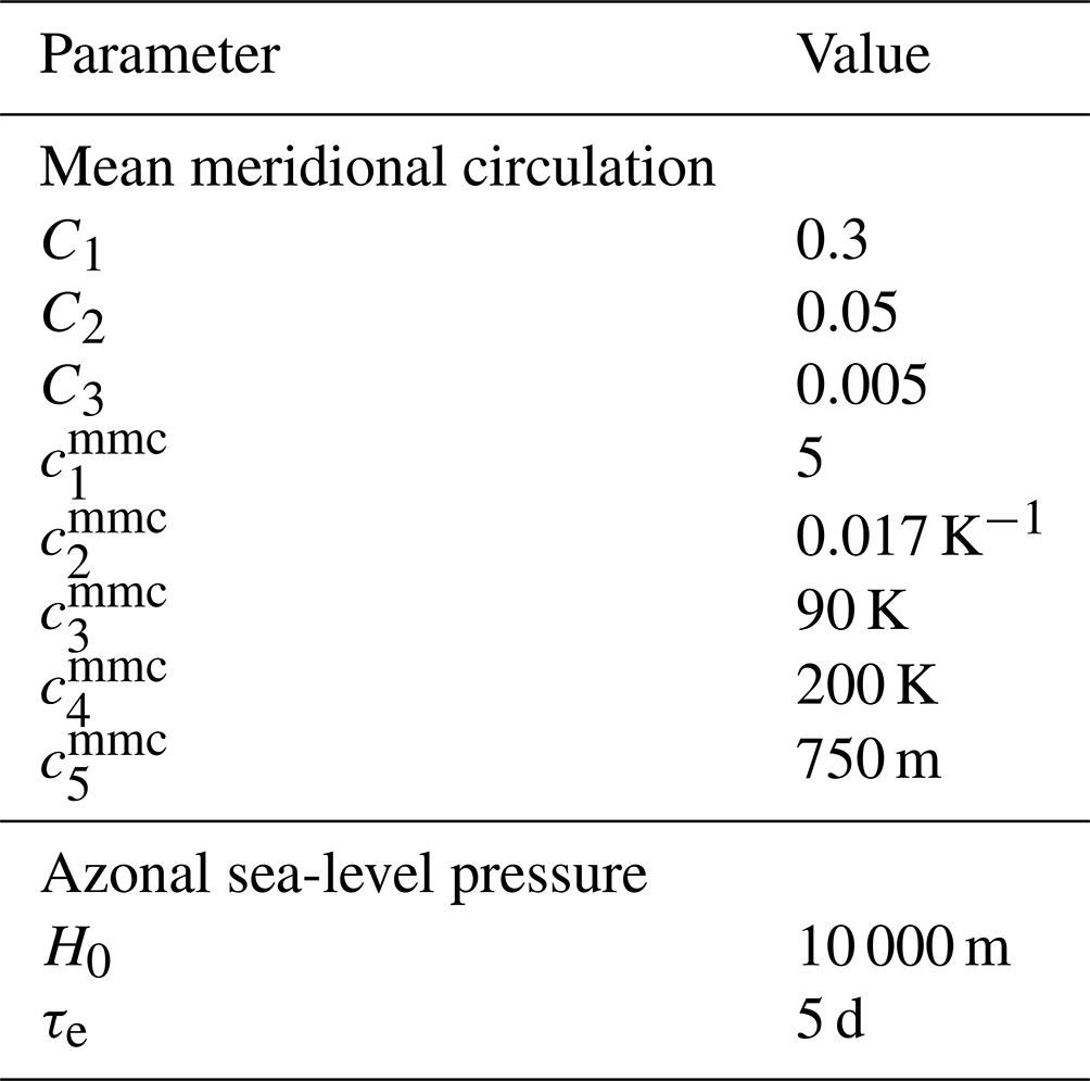
A3 Thermodynamics

The energy balance equation, vertically integrated from the surface to the top of the atmosphere, is written as

$$\begin{array}{}\text{(A40)}& \begin{array}{rl}& {\displaystyle \frac{\partial Q_{\mathrm{T}}}{\partial t}}=-{\displaystyle \frac{\mathrm{1}}{R_{\mathrm{e}}\cos \mathit{\varphi }}}\\ & \times \left[{\displaystyle \frac{\partial }{\partial \mathit{\lambda }}}\underset{z_{\mathrm{s}}}{\overset{H_{\mathrm{T}}}{\int }}\mathit{\rho }(u\mathit{\theta }+\widehat{u^{\prime }{\mathit{\theta }}^{\prime }})\mathrm{d}z+{\displaystyle \frac{\partial }{\partial \mathit{\varphi }}}\underset{z_{\mathrm{s}}}{\overset{H_{\mathrm{T}}}{\int }}\cos \mathit{\varphi }\mathit{\rho }(v\mathit{\theta }+\widehat{v^{\prime }{\mathit{\theta }}^{\prime }})\mathrm{d}z\right]\\ & +c_{\mathrm{v}}^{-\mathrm{1}}\left({\mathrm{SW}}_{\mathrm{a}}+{\mathrm{LW}}_{\mathrm{a}}+L_{\mathrm{e}}{P}_{\mathrm{w}}+L_{\mathrm{s}}{P}_{\mathrm{s}}+\mathrm{SH}\right),\end{array}\end{array}$$

where $Q_{\mathrm{T}}={\int }_{z_{\mathrm{s}}}^{H_{\mathrm{TOA}}}\mathit{\rho }T\mathrm{d}z$ is the heat content of the atmospheric column, SW_a is the shortwave radiation absorbed by the atmosphere, LW_a is the net atmosphere longwave radiation balance, P_w is rainfall and P_s is snowfall, L_e is the latent heat of evaporation and L_s the latent heat of sublimation, SH is the surface sensible heat flux, and c_v is the heat capacity of air at constant volume. The horizontal heat transport due to synoptic processes, $\widehat{u^{\prime }{\mathit{\theta }}^{\prime }}$ and $\widehat{v^{\prime }{\mathit{\theta }}^{\prime }}$, is represented as macroturbulent diffusion as described in Appendix A5. In CLIMBER-2 only the non-thermal wind is used in the energy balance equation, with the beta effect accounted for separately. This allowed a large time step of up to 1 d. Because the CLIMBER-X horizontal resolution is much higher than in CLIMBER-2, a relatively short time step of ∼ 2 h is needed, and with such a small time step the energy equation is stable even using the full wind vector. The energy balance equation is solved for T_a and the near-surface air temperature is diagnosed as

$$\begin{array}{}\text{(A41)}& T_{\mathrm{2}\mathrm{m}}={\displaystyle \frac{T_{\mathrm{a}}+T_{\star }}{\mathrm{2}}}.\end{array}$$

T_2 m is also the temperature that is used to compute the surface turbulent sensible heat flux.

A4 Hydrology

The water balance equation, vertically integrated from the surface to the top of the atmosphere, is written as

$$\begin{array}{}\text{(A42)}& \begin{array}{rl}& {\displaystyle \frac{\partial Q_{\mathrm{q}}}{\partial t}}=-{\displaystyle \frac{\mathrm{1}}{R_{\mathrm{e}}\cos \mathit{\varphi }}}\\ & \times \left[{\displaystyle \frac{\partial }{\partial \mathit{\lambda }}}\underset{z_{\mathrm{s}}}{\overset{H_{\mathrm{T}}}{\int }}\mathit{\rho }(uq+\widehat{u^{\prime }{q}^{\prime }})\mathrm{d}z+{\displaystyle \frac{\partial }{\partial \mathit{\varphi }}}\underset{z_{\mathrm{s}}}{\overset{H_{\mathrm{T}}}{\int }}\cos \mathit{\varphi }\mathit{\rho }(vq+\widehat{v^{\prime }{q}^{\prime }})\mathrm{d}z\right]\\ & +E-P,\end{array}\end{array}$$

where $Q_{\mathrm{q}}={\int }_{z_{\mathrm{s}}}^{H_{\mathrm{TOA}}}\mathit{\rho }q\mathrm{d}z$ is the water vapour content of the atmospheric column, E is surface evaporation and P is total precipitation. The horizontal moisture transport due to synoptic processes, $\widehat{u^{\prime }{q}^{\prime }}$ and $\widehat{v^{\prime }{q}^{\prime }}$, is represented as macroturbulent diffusion as described in Appendix A5.

The water balance equation is solved for q_a, and the near-surface air-specific humidity, which is used to compute the surface latent heat flux, is diagnosed as

$$\begin{array}{}\text{(A43)}& q_{\mathrm{2}\mathrm{m}}=r_{\mathrm{2}\mathrm{m}}\cdot q_{\mathrm{sat}}\left(T_{\mathrm{2}\mathrm{m}}\right),\end{array}$$

with $r_{\mathrm{2}\mathrm{m}}=(r_{\mathrm{a}}+r_{\star })/\mathrm{2}$ and $r_{\star }=q_{\mathrm{a}}/q_{\mathrm{sat}}\left(T_{\star }\right)$. Precipitation in the model is generated as follows:

$$\begin{array}{}\text{(A44)}& P=max\left(\mathrm{0},C+C_{\mathrm{slope}}+E\right){\displaystyle \frac{r_{\mathrm{a}}}{r_{\mathrm{a}}^{\max }}}+{\displaystyle \frac{Q_{\mathrm{q}}{r}_{\mathrm{a}}}{{\mathit{\tau }}_{\mathrm{p}}}},\end{array}$$

where C is moisture convergence into the atmospheric column by advection and diffusion and C_slope explicitly represents an additional moisture convergence due to synoptic activity on slopes. The first term on the right-hand side of Eq. (A44) represents a gradual removal of converging moisture by precipitation as atmospheric relative humidity increases, with all water entering an atmospheric column being added to precipitation when the atmospheric relative humidity reaches a maximum value $r_{\mathrm{a}}^{\max }$. The second term on the right-hand side of Eq. (A44) generates additional precipitation by removing atmospheric moisture with a given timescale τ_p and is applied only over land. The moisture convergence due to synoptic activity on slopes is computed assuming that moisture convergence is proportional to the vertical velocity induced by synoptic winds impacting on the slope:

$$\begin{array}{}\text{(A45)}& C_{\mathrm{slope}}=c_{\mathrm{slope}}^{\mathrm{p}}\sqrt{K}\left|\mathrm{\nabla }{z}_{\mathrm{s}}\right|{\mathit{\rho }}_{\mathrm{0}}{q}_{\mathrm{a}},\end{array}$$

where the synoptic wind is expressed through the eddy kinetic energy, K.

Table A3 Parameters for the hydrological cycle.

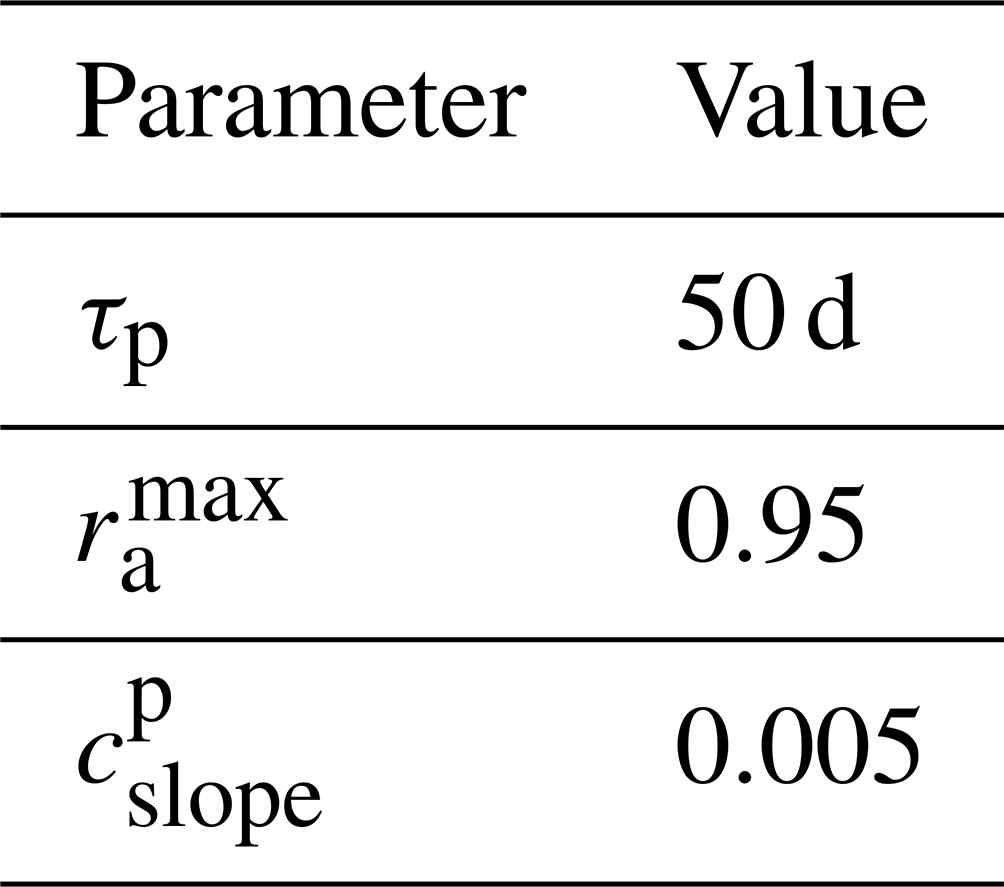
A5 Synoptic processes

Horizontal fluxes of energy and water originating from unresolved synoptic variability are represented as a macroturbulent diffusion process (Petoukhov et al., 2000):

$$\begin{array}{}\text{(A46)}& {\displaystyle }& {\displaystyle }\widehat{u^{\prime }{\mathit{\theta }}^{\prime }}=\widehat{u^{\prime }{T}^{\prime }}=-A_{\mathrm{T}}{\displaystyle \frac{\mathrm{1}}{R_{\mathrm{e}}\cos \mathit{\varphi }}}{\displaystyle \frac{\partial T}{\partial \mathit{\lambda }}},\text{(A47)}& {\displaystyle }& {\displaystyle }\widehat{v^{\prime }{\mathit{\theta }}^{\prime }}=\widehat{v^{\prime }{T}^{\prime }}=-A_{\mathrm{T}}{\displaystyle \frac{\mathrm{1}}{R_{\mathrm{e}}}}{\displaystyle \frac{\partial T}{\partial \mathit{\varphi }}},\text{(A48)}& {\displaystyle }& {\displaystyle }\widehat{u^{\prime }{q}^{\prime }}=-A_{\mathrm{q}}{\displaystyle \frac{\mathrm{1}}{R_{\mathrm{e}}\cos \mathit{\varphi }}}{\displaystyle \frac{\partial q}{\partial \mathit{\lambda }}},\text{(A49)}& {\displaystyle }& {\displaystyle }\widehat{v^{\prime }{q}^{\prime }}=-A_{\mathrm{q}}{\displaystyle \frac{\mathrm{1}}{R_{\mathrm{e}}}}{\displaystyle \frac{\partial q}{\partial \mathit{\varphi }}}.\end{array}$$

The diffusivities A_T and A_q are isotropic, are vertically uniform and depend on eddy kinetic energy K:

$$\begin{array}{}\text{(A50)}& {\displaystyle }& {\displaystyle }{A}_{\mathrm{T}}=c_{\mathrm{5}}^{\mathrm{syn}}\sqrt{K},\text{(A51)}& {\displaystyle }& {\displaystyle }{A}_{\mathrm{q}}=c_{\mathrm{6}}^{\mathrm{syn}}\cdot K.\end{array}$$

The different dependence of the diffusivities on eddy kinetic energy follows from Caballero and Hanley (2012).

The kinetic energy of synoptic eddies is described by an evolution equation:

$$\begin{array}{}\text{(A52)}& {\displaystyle \frac{\partial K}{\partial t}}=-\mathrm{\nabla }\cdot \left(\mathit{u}K\right)+\mathrm{\nabla }\left(A_{\mathrm{T}}\mathrm{\nabla }K\right)+P_{\mathrm{K}}-D_{\mathrm{K}}.\end{array}$$

Kinetic energy production is proportional to the maximum Eady model baroclinic growth rate (e.g. Hoskins and Valdes, 1990):

$$\begin{array}{}\text{(A53)}& P_{\mathrm{K}}=c_{\mathrm{1}}^{\mathrm{syn}}+c_{\mathrm{2}}^{\mathrm{syn}}{\displaystyle \frac{f}{N}}\left|{\displaystyle \frac{\partial \mathit{u}}{\partial z}}\right|,\end{array}$$

where the Brunt–Vaisala frequency N is defined as

$$\begin{array}{}\text{(A54)}& N=\sqrt{{\displaystyle \frac{g}{\mathit{\theta }}}{\displaystyle \frac{\partial \mathit{\theta }}{\partial z}}},\end{array}$$

and all vertical gradients are computed between 850 and 500 hPa. The dissipation of eddy kinetic energy is given by

$$\begin{array}{}\text{(A55)}& D_{\mathrm{K}}=\left(c_{\mathrm{3}}^{\mathrm{syn}}+c_{\mathrm{4}}^{\mathrm{syn}}{C}_{\mathrm{D}}\right)K^{\mathrm{3}/\mathrm{2}}.\end{array}$$

The synoptic component of near-surface wind is computed from eddy kinetic energy as follows:

$$\begin{array}{}\text{(A56)}& U_{\mathrm{syn}}=c_{\mathrm{7}}^{\mathrm{syn}}\mathit{ϵ}\cos \mathit{\alpha }\sqrt{K}.\end{array}$$

The synoptic vertical velocity at 700 hPa is calculated as

$$\begin{array}{}\text{(A57)}& w_{\mathrm{syn}}=c_{\mathrm{8}}^{\mathrm{syn}}\sqrt{K}.\end{array}$$

The module of surface wind, which is used for calculation of the turbulent surface fluxes, is defined as

$$\begin{array}{}\text{(A58)}& U_{\mathrm{s}}=\sqrt{u_{\mathrm{s}}^{\mathrm{2}}+v_{\mathrm{s}}^{\mathrm{2}}+U_{\mathrm{syn}}^{\mathrm{2}}},\end{array}$$

and the wind stress over the ocean is computed as

$$\begin{array}{}\text{(A59)}& {\displaystyle }& {\displaystyle }{\mathit{\tau }}_{\mathit{\lambda }}=C_{\mathrm{D}}{\mathit{\rho }}_{\mathrm{0}}{u}_{\mathrm{s}}{U}_{\mathrm{s}},\text{(A60)}& {\displaystyle }& {\displaystyle }{\mathit{\tau }}_{\mathit{\varphi }}=C_{\mathrm{D}}{\mathit{\rho }}_{\mathrm{0}}{v}_{\mathrm{s}}{U}_{\mathrm{s}}.\end{array}$$

Table A4 Parameters for synoptic processes.

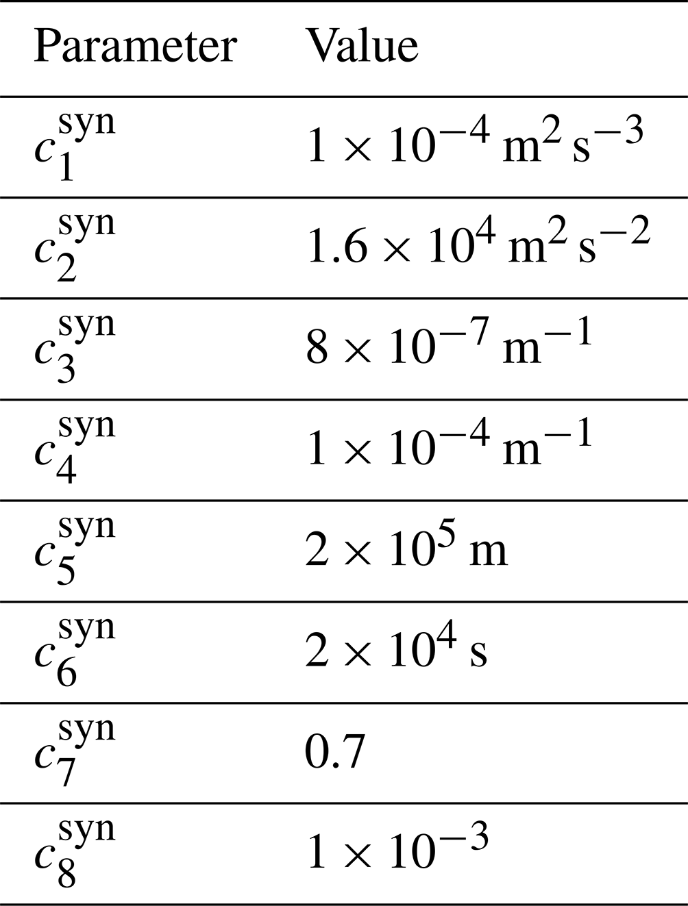
A6 Clouds

Total cloud cover fraction in SESAM is a combination of clouds related to atmospheric relative humidity and vertical velocity ($f_{\mathrm{cld}}^{\mathrm{r}}$) and clouds related to surface temperature inversion conditions ($f_{\mathrm{cld}}^{\mathrm{low}}$):

$$\begin{array}{}\text{(A61)}& f_{\mathrm{cld}}=\mathrm{1}-\left(\mathrm{1}-f_{\mathrm{cld}}^{\mathrm{r}}\right)\cdot \left(\mathrm{1}-f_{\mathrm{cld}}^{\mathrm{low}}\right).\end{array}$$

The relative humidity- and vertical-velocity-mediated cloud fraction, which provides the main contribution to cloud cover in the model, is given by

$$\begin{array}{}\text{(A62)}& f_{\mathrm{cld}}^{\mathrm{r}}=\left(c_{\mathrm{1}}^{\mathrm{cld}}+c_{\mathrm{2}}^{\mathrm{cld}}\tanh \left(c_{\mathrm{3}}^{\mathrm{cld}}{w}_{\mathrm{eff}}\right)\right)\cdot r_{\mathrm{a}}^{c_{\mathrm{4}}^{\mathrm{cld}}}.\end{array}$$

It is therefore proportional to $r_{\mathrm{a}}^{c_{\mathrm{cld}}^{\mathrm{4}}}$, with the proportionality factor depending on the effective vertical velocity at cloud level (w_eff). In addition to the mean vertical velocity, w_eff also includes contributions from vertical velocities resulting from synoptic disturbances and sub-grid-scale orography:

$$\begin{array}{}\text{(A63)}& w_{\mathrm{eff}}=w\left(\mathrm{700}\mathrm{hPa}\right)+c_{\mathrm{weff}}\cdot \left(w_{\mathrm{syn}}+w_{\mathrm{oro}}\right).\end{array}$$

The synoptic vertical velocity is given by Eq. (A57), while the orographic component is a function of surface wind speed and grid cell standard deviation of surface elevation (σ_oro):

$$\begin{array}{}\text{(A64)}& w_{\mathrm{oro}}=c_{\mathrm{woro}}{U}_{\mathrm{s}}{\mathit{\sigma }}_{\mathrm{oro}}.\end{array}$$

The fraction of low clouds related to the presence of surface temperature inversion, when $r_{\star }>r_{\mathrm{a}}$, is defined as

$$\begin{array}{}\text{(A65)}& f_{\mathrm{cld}}^{\mathrm{low}}=c_{\mathrm{5}}^{\mathrm{cld}}{f}_{\mathrm{freezedry}}{\displaystyle \frac{(r_{\star }-r_{\mathrm{a}})+c_{\mathrm{6}}^{\mathrm{cld}}}{\mathrm{2}{c}_{\mathrm{6}}^{\mathrm{cld}}}}\cdot r_{\mathrm{a}}^{c_{\mathrm{4}}^{\mathrm{cld}}}.\end{array}$$

The factor f_freezedry represents the freeze-dry mechanism following Vavrus and Waliser (2008) and decreases the low cloud amount in very cold and dry conditions,

$$\begin{array}{}\text{(A66)}& f_{\mathrm{freezedry}}=\mathrm{0.1}+\mathrm{0.9}{\displaystyle \frac{q_{\mathrm{a}}}{c_{\mathrm{7}}^{\mathrm{cld}}}},\end{array}$$

and is limited to the range [0,1].

The cloud base height is assumed to coincide with the top of the planetary boundary layer, H_pbl. Cloud top height follows the height of the tropopause, modified by a factor depending on the mean vertical velocity at 700 hPa:

$$\begin{array}{}\text{(A67)}& H_{\mathrm{cld}}=c_{\mathrm{1}}^{\mathrm{hcld}}+c_{\mathrm{2}}^{\mathrm{hcld}}{H}_{\mathrm{T}}\cdot \left(\mathrm{1}+c_{\mathrm{3}}^{\mathrm{hcld}}w\left(\mathrm{700}\mathrm{hPa}\right)\right).\end{array}$$

Cloud optical thickness is parameterized as a function of surface air temperature, cloud fraction and column water content,

$$\begin{array}{}\text{(A68)}& {\mathit{\tau }}_{\mathrm{cld}}=c_{\mathrm{3}}^{\mathit{\tau }}\left[\mathrm{1}+\tanh \left(-{\displaystyle \frac{T_{\mathrm{2}\mathrm{m}}-T_{\mathrm{0}}-c_{\mathrm{1}}^{\mathit{\tau }}}{c_{\mathrm{2}}^{\mathit{\tau }}}}\right)\right]{\left(f_{\mathrm{cld}}{Q}_{\mathrm{q}}\right)}^{c_{\mathrm{4}}^{\mathit{\tau }}},\end{array}$$

and is further modified to account for the indirect effect of sulfate aerosols following Bauer et al. (2008).

Table A5 Cloud parameters.

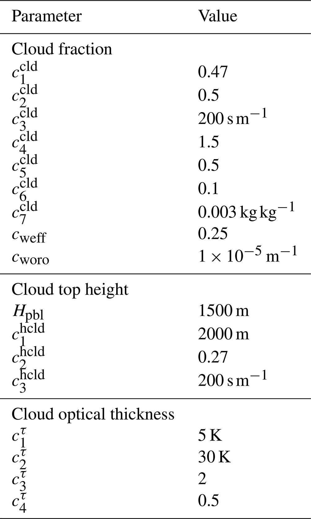
A7 Shortwave radiation

The computation of shortwave radiation fluxes is based on a two-stream delta-Eddington approximation of the transport equation in a gas–aerosol atmosphere (see Petoukhov et al., 2003, for a more detailed description). The net downward shortwave radiation fluxes are computed at the top of the atmosphere and at the surface as a weighted mean of clear-sky (cs) and cloudy (cld) fluxes:

$$\begin{array}{}\text{(A69)}& {\displaystyle }& {\displaystyle }{\mathrm{SW}}_{\mathrm{top}}=f_{\mathrm{cld}}{\mathrm{SW}}_{\mathrm{top}}^{\mathrm{cld}}+(\mathrm{1}-f_{\mathrm{cld}}){\mathrm{SW}}_{\mathrm{top}}^{\mathrm{cs}},\text{(A70)}& {\displaystyle }& {\displaystyle }{\mathrm{SW}}_{\mathrm{sur}}=f_{\mathrm{cld}}{\mathrm{SW}}_{\mathrm{sur}}^{\mathrm{cld}}+(\mathrm{1}-f_{\mathrm{cld}}){\mathrm{SW}}_{\mathrm{sur}}^{\mathrm{cs}}.\end{array}$$

The clear-sky and cloudy fluxes are computed separately for two spectral bands – visible (vu) and near-infrared (ir) – and for each macro surface type. The individual components of the shortwave radiation flux are computed as

$$\begin{array}{}\text{(A71)}& {\displaystyle }{\mathrm{SW}}_{\mathrm{top}}^{\mathrm{cs}}={\mathrm{SW}}_{\mathrm{top}}^{\downarrow }-{\mathrm{SW}}_{\mathrm{top}}^{\downarrow }(f_{\mathrm{vu}}{\mathit{\alpha }}_{\mathrm{atm},\mathrm{vu}}^{\mathrm{cs}}+(\mathrm{1}-f_{\mathrm{vu}}\left){\mathit{\alpha }}_{\mathrm{atm},\mathrm{ir}}^{\mathrm{cs}}\right),\text{(A72)}& {\displaystyle }{\mathrm{SW}}_{\mathrm{top}}^{\mathrm{cld}}={\mathrm{SW}}_{\mathrm{top}}^{\downarrow }-{\mathrm{SW}}_{\mathrm{top}}^{\downarrow }(f_{\mathrm{vu}}{\mathit{\alpha }}_{\mathrm{atm},\mathrm{vu}}^{\mathrm{cld}}+(\mathrm{1}-f_{\mathrm{vu}}\left){\mathit{\alpha }}_{\mathrm{atm},\mathrm{ir}}^{\mathrm{cld}}\right),\text{(A73)}& {\displaystyle }{\mathrm{SW}}_{\mathrm{sur}}^{\mathrm{cs}}={\mathrm{SW}}_{\mathrm{top}}^{\downarrow }(f_{\mathrm{vu}}{I}_{\mathrm{atm},\mathrm{vu}}^{\mathrm{cs}}+(\mathrm{1}-f_{\mathrm{vu}}\left)I_{\mathrm{atm},\mathrm{ir}}^{\mathrm{cs}}\right),\text{(A74)}& {\displaystyle }{\mathrm{SW}}_{\mathrm{sur}}^{\mathrm{cld}}={\mathrm{SW}}_{\mathrm{top}}^{\downarrow }(f_{\mathrm{vu}}{I}_{\mathrm{atm},\mathrm{vu}}^{\mathrm{cld}}+(\mathrm{1}-f_{\mathrm{vu}}\left)I_{\mathrm{atm},\mathrm{ir}}^{\mathrm{cld}}\right),\end{array}$$

where f_vu is the fraction of solar radiation in the visible and ultraviolet spectral range, α_atm is the planetary albedo and I_atm is the atmosphere integral transmission function. Planetary albedos used to compute the net shortwave fluxes at TOA are defined as

$$\begin{array}{}\text{(A75)}& {\displaystyle }\begin{array}{rl}{\mathit{\alpha }}_{\mathrm{atm},\mathrm{vu}}^{\mathrm{cs}}& =\left({\mathit{\alpha }}_{\mathrm{sct},\mathrm{vu}}+{\displaystyle \frac{(\mathrm{1}-{\mathit{\alpha }}_{\mathrm{sct},\mathrm{vu}}{)}^{\mathrm{2}}{\mathit{\alpha }}_{\mathrm{sur},\mathrm{vu}}^{\mathrm{cs}}}{\mathrm{1}-{\mathit{\alpha }}_{\mathrm{sct},\mathrm{vu}}{\mathit{\alpha }}_{\mathrm{sur},\mathrm{vu}}^{\mathrm{cs}}}}\right)\\ & \times I_{\mathrm{wv},\mathrm{vu}}^{\mathrm{cs}}{I}_{\mathrm{aer},\mathrm{vu}}^{\mathrm{cs}}{I}_{{\mathrm{O}}_{\mathrm{3}},\mathrm{vu}},\end{array}\text{(A76)}& {\displaystyle }\begin{array}{rl}{\mathit{\alpha }}_{\mathrm{atm},\mathrm{ir}}^{\mathrm{cs}}& =\left({\mathit{\alpha }}_{\mathrm{sct},\mathrm{ir}}+{\displaystyle \frac{(\mathrm{1}-{\mathit{\alpha }}_{\mathrm{sct},\mathrm{ir}}{)}^{\mathrm{2}}{\mathit{\alpha }}_{\mathrm{sur},\mathrm{ir}}^{\mathrm{cs}}}{\mathrm{1}-{\mathit{\alpha }}_{\mathrm{sct},\mathrm{ir}}{\mathit{\alpha }}_{\mathrm{sur},\mathrm{ir}}^{\mathrm{cs}}}}\right)\\ & \times I_{\mathrm{wv},\mathrm{ir}}^{\mathrm{cs}}{I}_{\mathrm{aer},\mathrm{ir}}^{\mathrm{cs}}{I}_{{\mathrm{O}}_{\mathrm{3}},\mathrm{ir}},\end{array}\text{(A77)}& {\displaystyle }\begin{array}{rl}{\mathit{\alpha }}_{\mathrm{atm},\mathrm{vu}}^{\mathrm{cld}}& =\left({\mathit{\alpha }}_{\mathrm{cld},\mathrm{vu}}+{\displaystyle \frac{(\mathrm{1}-{\mathit{\alpha }}_{\mathrm{cld},\mathrm{vu}}{)}^{\mathrm{2}}{\mathit{\alpha }}_{\mathrm{sur},\mathrm{vu}}^{\mathrm{cld}}}{\mathrm{1}-{\mathit{\alpha }}_{\mathrm{cld},\mathrm{vu}}{\mathit{\alpha }}_{\mathrm{sur},\mathrm{vu}}^{\mathrm{cld}}}}\right)\\ & \times I_{\mathrm{wv},\mathrm{vu}}^{\mathrm{cld}}{I}_{\mathrm{aer},\mathrm{vu}}^{\mathrm{cld}}{I}_{{\mathrm{O}}_{\mathrm{3}},\mathrm{vu}}{I}_{\mathrm{cld},\mathrm{vu}},\end{array}\text{(A78)}& {\displaystyle }\begin{array}{rl}{\mathit{\alpha }}_{\mathrm{atm},\mathrm{ir}}^{\mathrm{cld}}& =\left({\mathit{\alpha }}_{\mathrm{cld},\mathrm{ir}}+{\displaystyle \frac{(\mathrm{1}-{\mathit{\alpha }}_{\mathrm{cld},\mathrm{ir}}{)}^{\mathrm{2}}{\mathit{\alpha }}_{\mathrm{sur},\mathrm{ir}}^{\mathrm{cld}}}{\mathrm{1}-{\mathit{\alpha }}_{\mathrm{cld},\mathrm{ir}}{\mathit{\alpha }}_{\mathrm{sur},\mathrm{ir}}^{\mathrm{cld}}}}\right)\\ & \times I_{\mathrm{wv},\mathrm{ir}}^{\mathrm{cld}}{I}_{\mathrm{aer},\mathrm{ir}}^{\mathrm{cld}}{I}_{{\mathrm{O}}_{\mathrm{3}},\mathrm{ir}}{I}_{\mathrm{cld},\mathrm{ir}}.\end{array}\end{array}$$

The atmospheric scattering albedo depends on the cosine of the solar zenith angle (μ) and the optical thickness (τ_aer) and imaginary part of the refractive index ($R_{\mathrm{aer}}^{\mathrm{im}}$) of the aerosol load:

$$\begin{array}{}\text{(A79)}& {\displaystyle }\begin{array}{rl}{\mathit{\alpha }}_{\mathrm{sct},\mathrm{vu}}& =\mathrm{1}-(\mathrm{1}-r_{\mathrm{sct}})\exp (-{\mathit{\mu }}^{{\mathrm{p}}_{\mathrm{1}}}{\left(\mathrm{0.55}{\mathit{\tau }}_{\mathrm{aer}}\right)}^{{\mathrm{p}}_{\mathrm{2}}}\\ & \times \left({\mathit{\alpha }}_{\mathrm{1}}-{\mathit{\alpha }}_{\mathrm{2}}\log (\mathrm{1}+{\mathit{\alpha }}_{\mathrm{3}}{R}_{\mathrm{aer}}^{\mathrm{im}})\right)),\end{array}\text{(A80)}& {\displaystyle }\begin{array}{rl}{\mathit{\alpha }}_{\mathrm{sct},\mathrm{ir}}& =\mathrm{1}-\exp (-{\mathit{\mu }}^{{\mathrm{p}}_{\mathrm{1}}}{\left(\mathrm{0.55}{\mathit{\tau }}_{\mathrm{aer}}\right)}^{{\mathrm{p}}_{\mathrm{2}}}\\ & \times \left({\mathit{\alpha }}_{\mathrm{1}}-{\mathit{\alpha }}_{\mathrm{2}}\log (\mathrm{1}+{\mathit{\alpha }}_{\mathrm{3}}{R}_{\mathrm{aer}}^{\mathrm{im}})\right)).\end{array}\end{array}$$

Cloud albedo is computed from cloud optical thickness as follows:

$$\begin{array}{}\text{(A81)}& {\displaystyle }& {\displaystyle }{\mathit{\alpha }}_{\mathrm{cld},\mathrm{vu}}=\mathrm{1}-(\mathrm{1}-{\mathit{\alpha }}_{\mathrm{sct},\mathrm{vu}})\exp (-g_{\mathrm{cld}}{\displaystyle \frac{{\mathit{\tau }}_{\mathrm{cld}}^{p_{\mathrm{4}}}}{{\mathit{\mu }}^{p_{\mathrm{3}}}}}),\text{(A82)}& {\displaystyle }& {\displaystyle }{\mathit{\alpha }}_{\mathrm{cld},\mathrm{ir}}=\mathrm{1}-(\mathrm{1}-{\mathit{\alpha }}_{\mathrm{sct},\mathrm{ir}})\exp (-g_{\mathrm{cld}}{\displaystyle \frac{{\mathit{\tau }}_{\mathrm{cld}}^{p_{\mathrm{4}}}}{{\mathit{\mu }}^{p_{\mathrm{3}}}}}).\end{array}$$

The atmospheric integral transmission functions used to derive the net shortwave fluxes at the surface are calculated as

$$\begin{array}{}\text{(A83)}& {\displaystyle }\begin{array}{rl}{I}_{\mathrm{atm},\mathrm{vu}}^{\mathrm{cs}}& =(\mathrm{1}-{\mathit{\alpha }}_{\mathrm{sct},\mathrm{vu}})(\mathrm{1}-{\mathit{\alpha }}_{\mathrm{sur},\mathrm{vu}}^{\mathrm{cs}})I_{\mathrm{wv},\mathrm{vu}}^{\mathrm{cs},\mathrm{1}}{I}_{\mathrm{aer},\mathrm{vu}}^{\mathrm{cs},\mathrm{1}}{I}_{{\mathrm{O}}_{\mathrm{3}},\mathrm{vu}}\\ & +(\mathrm{1}-{\mathit{\alpha }}_{\mathrm{sct},\mathrm{vu}}){\mathit{\alpha }}_{\mathrm{sur},\mathrm{vu}}^{\mathrm{cs}}{\mathit{\alpha }}_{\mathrm{sct},\mathrm{vu}}^{\mathrm{0}}\\ & \times {\displaystyle \frac{\mathrm{1}-{\mathit{\alpha }}_{\mathrm{sur},\mathrm{vu}}^{\mathrm{cs}}}{\mathrm{1}-{\mathit{\alpha }}_{\mathrm{sct},\mathrm{vu}}^{\mathrm{0}}{\mathit{\alpha }}_{\mathrm{sur},\mathrm{vu}}^{\mathrm{cs}}}}{I}_{\mathrm{wv},\mathrm{vu}}^{\mathrm{cs},\mathrm{2}}{I}_{\mathrm{aer},\mathrm{vu}}^{\mathrm{cs},\mathrm{2}}{I}_{{\mathrm{O}}_{\mathrm{3}},\mathrm{vu}},\end{array}\text{(A84)}& {\displaystyle }\begin{array}{rl}{I}_{\mathrm{atm},\mathrm{ir}}^{\mathrm{cs}}& =(\mathrm{1}-{\mathit{\alpha }}_{\mathrm{sct},\mathrm{ir}})(\mathrm{1}-{\mathit{\alpha }}_{\mathrm{sur},\mathrm{ir}}^{\mathrm{cs}})I_{\mathrm{wv},\mathrm{ir}}^{\mathrm{cs},\mathrm{1}}{I}_{\mathrm{aer},\mathrm{ir}}^{\mathrm{cs},\mathrm{1}}{I}_{{\mathrm{O}}_{\mathrm{3}},\mathrm{ir}}\\ & +(\mathrm{1}-{\mathit{\alpha }}_{\mathrm{sct},\mathrm{ir}}){\mathit{\alpha }}_{\mathrm{sur},\mathrm{ir}}^{\mathrm{cs}}{\mathit{\alpha }}_{\mathrm{sct},\mathrm{ir}}^{\mathrm{0}}\\ & \times {\displaystyle \frac{\mathrm{1}-{\mathit{\alpha }}_{\mathrm{sur},\mathrm{ir}}^{\mathrm{cs}}}{\mathrm{1}-{\mathit{\alpha }}_{\mathrm{sct},\mathrm{ir}}^{\mathrm{0}}{\mathit{\alpha }}_{\mathrm{sur},\mathrm{ir}}^{\mathrm{cs}}}}{I}_{\mathrm{wv},\mathrm{ir}}^{\mathrm{cs},\mathrm{2}}{I}_{\mathrm{aer},\mathrm{ir}}^{\mathrm{cs},\mathrm{2}}{I}_{{\mathrm{O}}_{\mathrm{3}},\mathrm{ir}},\end{array}\text{(A85)}& {\displaystyle }\begin{array}{rl}{I}_{\mathrm{atm},\mathrm{vu}}^{\mathrm{cld}}& =(\mathrm{1}-{\mathit{\alpha }}_{\mathrm{cld},\mathrm{vu}})(\mathrm{1}-{\mathit{\alpha }}_{\mathrm{sur},\mathrm{vu}}^{\mathrm{cld}})I_{\mathrm{cld},\mathrm{vu}}^{\mathrm{1}}{I}_{\mathrm{wv},\mathrm{vu}}^{\mathrm{cld},\mathrm{1}}{I}_{\mathrm{aer},\mathrm{vu}}^{\mathrm{cld},\mathrm{1}}{I}_{{\mathrm{O}}_{\mathrm{3}},\mathrm{vu}}\\ & +(\mathrm{1}-{\mathit{\alpha }}_{\mathrm{cld},\mathrm{vu}}){\mathit{\alpha }}_{\mathrm{sur},\mathrm{vu}}^{\mathrm{cld}}{\mathit{\alpha }}_{\mathrm{cld},\mathrm{vu}}\\ & \times {\displaystyle \frac{\mathrm{1}-{\mathit{\alpha }}_{\mathrm{sur},\mathrm{vu}}^{\mathrm{cld}}}{\mathrm{1}-{\mathit{\alpha }}_{\mathrm{cld},\mathrm{vu}}{\mathit{\alpha }}_{\mathrm{sur},\mathrm{vu}}^{\mathrm{cld}}}}{I}_{\mathrm{cld},\mathrm{vu}}^{\mathrm{2}}{I}_{\mathrm{wv},\mathrm{vu}}^{\mathrm{cld},\mathrm{2}}{I}_{\mathrm{aer},\mathrm{vu}}^{\mathrm{cld},\mathrm{2}}{I}_{{\mathrm{O}}_{\mathrm{3}},\mathrm{vu}},\end{array}\text{(A86)}& {\displaystyle }\begin{array}{rl}{I}_{\mathrm{atm},\mathrm{ir}}^{\mathrm{cld}}& =(\mathrm{1}-{\mathit{\alpha }}_{\mathrm{cld},\mathrm{ir}})(\mathrm{1}-{\mathit{\alpha }}_{\mathrm{sur},\mathrm{ir}}^{\mathrm{cld}})I_{\mathrm{cld},\mathrm{ir}}^{\mathrm{1}}{I}_{\mathrm{wv},\mathrm{ir}}^{\mathrm{cld},\mathrm{1}}{I}_{\mathrm{aer},\mathrm{ir}}^{\mathrm{cld},\mathrm{1}}{I}_{{\mathrm{O}}_{\mathrm{3}},\mathrm{ir}}\\ & +(\mathrm{1}-{\mathit{\alpha }}_{\mathrm{cld},\mathrm{ir}}){\mathit{\alpha }}_{\mathrm{sur},\mathrm{ir}}^{\mathrm{cld}}{\mathit{\alpha }}_{\mathrm{cld},\mathrm{ir}}\\ & \times {\displaystyle \frac{\mathrm{1}-{\mathit{\alpha }}_{\mathrm{sur},\mathrm{ir}}^{\mathrm{cld}}}{\mathrm{1}-{\mathit{\alpha }}_{\mathrm{cld},\mathrm{ir}}{\mathit{\alpha }}_{\mathrm{sur},\mathrm{ir}}^{\mathrm{cld}}}}{I}_{\mathrm{cld},\mathrm{ir}}^{\mathrm{2}}{I}_{\mathrm{wv},\mathrm{ir}}^{\mathrm{cld},\mathrm{2}}{I}_{\mathrm{aer},\mathrm{ir}}^{\mathrm{cld},\mathrm{2}}{I}_{{\mathrm{O}}_{\mathrm{3}},\mathrm{ir}}.\end{array}\end{array}$$

The first terms on the right-hand side represent the direct effect on radiation reaching the surface, while the second terms represent the effect of multiple reflections between the surface and atmospheric scatterers and clouds.

The integral transmission functions for water vapour, aerosols, ozone and clouds are given by

$$\begin{array}{}\text{(A87)}& {\displaystyle }& {\displaystyle }{I}_{\mathrm{wv},\mathrm{uv}}=a_{\mathrm{1}}^{\mathrm{wv}}\exp (-b_{\mathrm{1}}^{\mathrm{wv}}{M}_{\mathrm{wv}})+a_{\mathrm{2}}^{\mathrm{wv}}\exp (-b_{\mathrm{2}}^{\mathrm{wv}}{M}_{\mathrm{wv}}),\text{(A88)}& {\displaystyle }& {\displaystyle }{I}_{\mathrm{wv},\mathrm{ir}}=\mathrm{1},\text{(A89)}& {\displaystyle }& {\displaystyle }{I}_{\mathrm{aer},\mathrm{vu}}=I_{\mathrm{aer},\mathrm{ir}}=\exp (-{\mathit{\gamma }}_{\mathrm{1}}^{\mathrm{aer}}{M}_{\mathrm{aer}}(R_{\mathrm{aer}}^{\mathrm{im}}{)}^{{\mathit{\gamma }}_{\mathrm{2}}^{\mathrm{aer}}}),\text{(A90)}& {\displaystyle }& {\displaystyle }{I}_{{\mathrm{O}}_{\mathrm{3}},\mathrm{uv}}=\mathrm{0.96},\text{(A91)}& {\displaystyle }& {\displaystyle }{I}_{{\mathrm{O}}_{\mathrm{3}},\mathrm{ir}}=\mathrm{1},\text{(A92)}& {\displaystyle }& {\displaystyle }{I}_{\mathrm{cld},\mathrm{uv}}=\mathrm{0.9},\text{(A93)}& {\displaystyle }& {\displaystyle }{I}_{\mathrm{cld},\mathrm{ir}}=\mathrm{0.9},\end{array}$$

where M_w and M_aer are the effective absorber mass of water and aerosols in the column, respectively. In general, M_w and M_aer are different for clear sky and cloudy sky and for the top of the atmosphere and the surface:

$$\begin{array}{}\text{(A94)}& {\displaystyle }{M}_{\mathrm{w}}^{\mathrm{cs}}=\left({\displaystyle \frac{\mathrm{1}}{\mathit{\mu }}}+{\displaystyle \frac{\mathrm{1}}{{\mathit{\mu }}_{\mathrm{0}}}}\right)W,\text{(A95)}& {\displaystyle }{M}_{\mathrm{w}}^{\mathrm{cs},\mathrm{1}}={\displaystyle \frac{\mathrm{1}}{\mathit{\mu }}}W,\text{(A96)}& {\displaystyle }{M}_{\mathrm{w}}^{\mathrm{cs},\mathrm{2}}=M_{\mathrm{w}}^{\mathrm{cs},\mathrm{1}}+\left(\mathrm{1}-e^{-\mathrm{0.25}}\right){\displaystyle \frac{\mathrm{2}}{{\mathit{\mu }}_{\mathrm{0}}}}W,\text{(A97)}& {\displaystyle }{M}_{\mathrm{w}}^{\mathrm{cld}}=e^{-H_{\mathrm{cld}}/H_{\mathrm{q}}}\left({\displaystyle \frac{\mathrm{1}}{\mathit{\mu }}}+{\displaystyle \frac{\mathrm{1}}{{\mathit{\mu }}_{\mathrm{0}}}}+\left(\mathrm{1}-e^{D_{\mathrm{cld}}/H_{\mathrm{q}}}\right)\right)W,\text{(A98)}& {\displaystyle }{M}_{\mathrm{w}}^{\mathrm{cld},\mathrm{1}}=\left[e^{-H_{\mathrm{cld}}/H_{\mathrm{q}}}{\displaystyle \frac{\mathrm{1}}{\mathit{\mu }}}+f_{\exp }^{\mathrm{1}}+f_{\exp }^{\mathrm{2}}\right]W,\text{(A99)}& {\displaystyle }{M}_{\mathrm{w}}^{\mathrm{cld},\mathrm{2}}=M_{\mathrm{w}}^{\mathrm{cld},\mathrm{1}}+\left(f_{\exp }^{\mathrm{1}}+\mathrm{2}{f}_{\exp }^{\mathrm{2}}\right)W,\text{(A100)}& {\displaystyle }{M}_{\mathrm{aer}}^{\mathrm{cs}}=\left({\displaystyle \frac{\mathrm{1}}{\mathit{\mu }}}+{\displaystyle \frac{\mathrm{1}}{{\mathit{\mu }}_{\mathrm{0}}}}\right)\mathrm{0.55}{\mathit{\tau }}_{\mathrm{aer}},\text{(A101)}& {\displaystyle }{M}_{\mathrm{aer}}^{\mathrm{cs},\mathrm{1}}={\displaystyle \frac{\mathrm{1}}{\mathit{\mu }}}\mathrm{0.55}{\mathit{\tau }}_{\mathrm{aer}},\text{(A102)}& {\displaystyle }{M}_{\mathrm{aer}}^{\mathrm{cs},\mathrm{2}}=M_{\mathrm{aer}}^{\mathrm{cs},\mathrm{1}}+\left(\mathrm{1}-e^{-\mathrm{0.25}}\right){\displaystyle \frac{\mathrm{2}}{{\mathit{\mu }}_{\mathrm{0}}}}\mathrm{0.55}{\mathit{\tau }}_{\mathrm{aer}},\text{(A103)}& {\displaystyle }{M}_{\mathrm{aer}}^{\mathrm{cld}}=e^{-H_{\mathrm{cld}}/H_{\mathrm{q}}}\left({\displaystyle \frac{\mathrm{1}}{\mathit{\mu }}}+{\displaystyle \frac{\mathrm{1}}{{\mathit{\mu }}_{\mathrm{0}}}}+\left(\mathrm{1}-e^{D_{\mathrm{cld}}/H_{\mathrm{q}}}\right)\right)\mathrm{0.55}{\mathit{\tau }}_{\mathrm{aer}},\text{(A104)}& {\displaystyle }{M}_{\mathrm{aer}}^{\mathrm{cld},\mathrm{1}}=\left[e^{-H_{\mathrm{cld}}/H_{\mathrm{q}}}{\displaystyle \frac{\mathrm{1}}{\mathit{\mu }}}+f_{\exp }^{\mathrm{1}}+f_{\exp }^{\mathrm{2}}\right]\mathrm{0.55}{\mathit{\tau }}_{\mathrm{aer}},\text{(A105)}& {\displaystyle }{M}_{\mathrm{aer}}^{\mathrm{cld},\mathrm{2}}=M_{\mathrm{aer}}^{\mathrm{cld},\mathrm{1}}+\left(f_{\exp }^{\mathrm{1}}+\mathrm{2}{f}_{\exp }^{\mathrm{2}}\right)\mathrm{0.55}{\mathit{\tau }}_{\mathrm{aer}}.\end{array}$$

W is the column water content in g cm⁻² and μ₀ is the effective cosine of the zenith angle for diffuse radiation, H_q is the humidity height scale, D_cld is the geometrical thickness of clouds, $f_{\exp }^{\mathrm{1}}=\exp (-H_{\mathrm{cld}}/H_{\mathrm{q}})-\exp (-(H_{\mathrm{cld}}+D_{\mathrm{cld}})/H_{\mathrm{q}})$ and $f_{\exp }^{\mathrm{2}}=\mathrm{1}-\exp (-H_{\mathrm{cld}}/H_{\mathrm{q}})/{\mathit{\mu }}_{\mathrm{0}}$.

Shortwave radiation parameters are tuned in offline mode using prescribed column water content, surface albedo and total cloud cover fraction from ERA-Interim reanalysis (Dee et al., 2011) and cloud top height and cloud optical thickness from the ISCCP climatology (Rossow and Schiffer, 1999). The target is to minimize the root mean square error in top-of-the-atmosphere and surface shortwave radiation fluxes for clear sky and total sky. The resulting zonal mean net top-of-the-atmosphere shortwave radiation is shown in Figs. A1 and A2 for clear sky and total sky, respectively.

Additional constraints on model parameters are provided by the shortwave radiative kernels at the top of the atmosphere and at the surface, which are available for several climate models (Shell et al., 2008; Block and Mauritsen, 2013; Smith et al., 2018; Pendergrass et al., 2018). The TOA kernels computed using the CLIMBER-X shortwave radiation code are compared to those available from the different climate models in Fig. A3. The sensitivity of TOA shortwave flux to changes in surface albedo is well captured by the shortwave radiation scheme of CLIMBER-X (Fig. A3a), while the sensitivity to water vapour changes is too large in the tropics (Fig. A3b). Note, however, that changes in water vapour have a generally small effect on TOA shortwave radiation, so that this bias is expected to have only minor implications for model results.

Table A6 Shortwave radiation parameters.

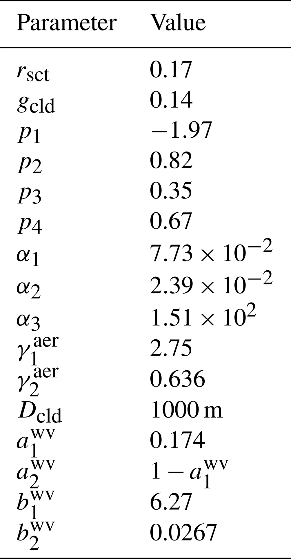
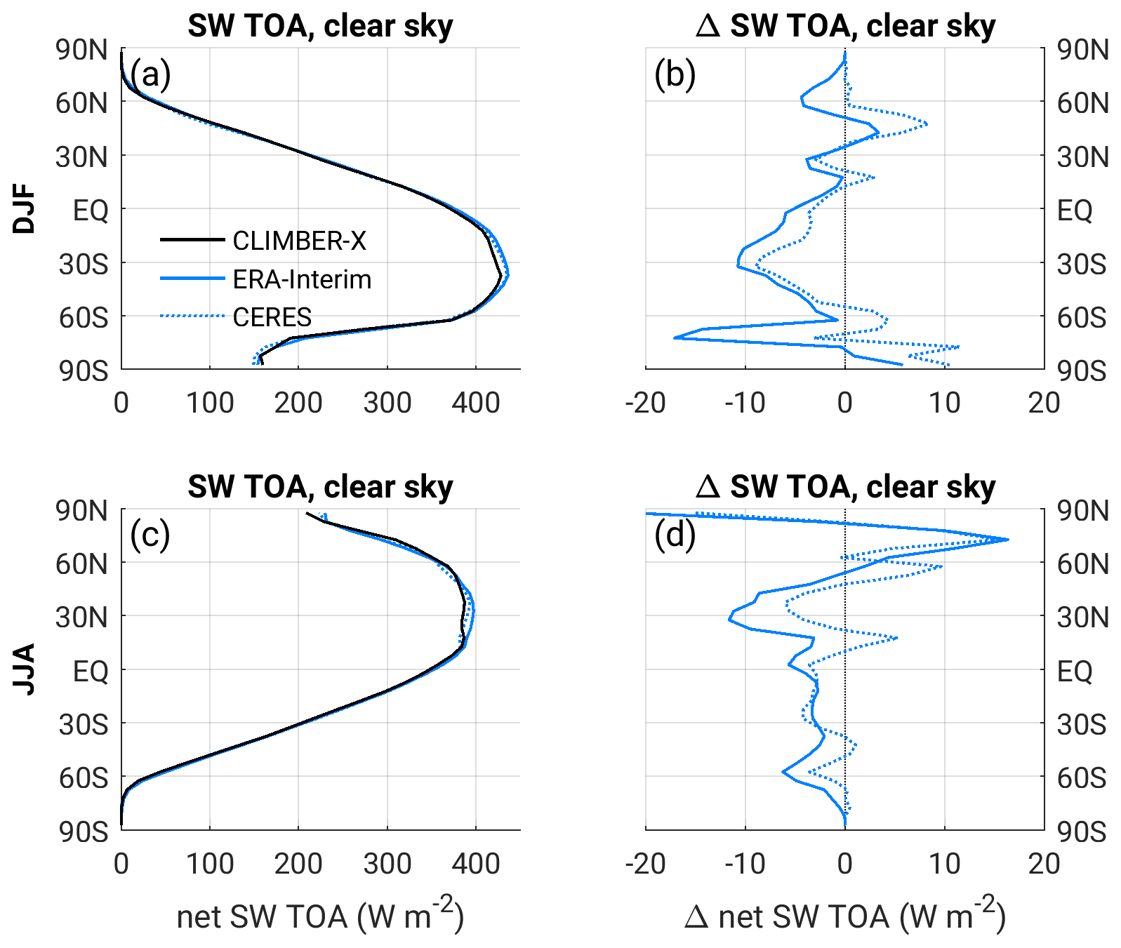
Figure A1 Zonal mean net shortwave radiation at the top of the atmosphere for clear-sky conditions as computed by the CLIMBER-X radiation code in the offline set-up compared to ERA-Interim reanalysis (Dee et al., 2011) and CERES satellite observations (Loeb et al., 2018). Panels (a) and (b) are for December–January–February and panels (c) and (d) are for June–July–August. Panels (a) and (c) show absolute values, while panels (b) and (d) show model biases.

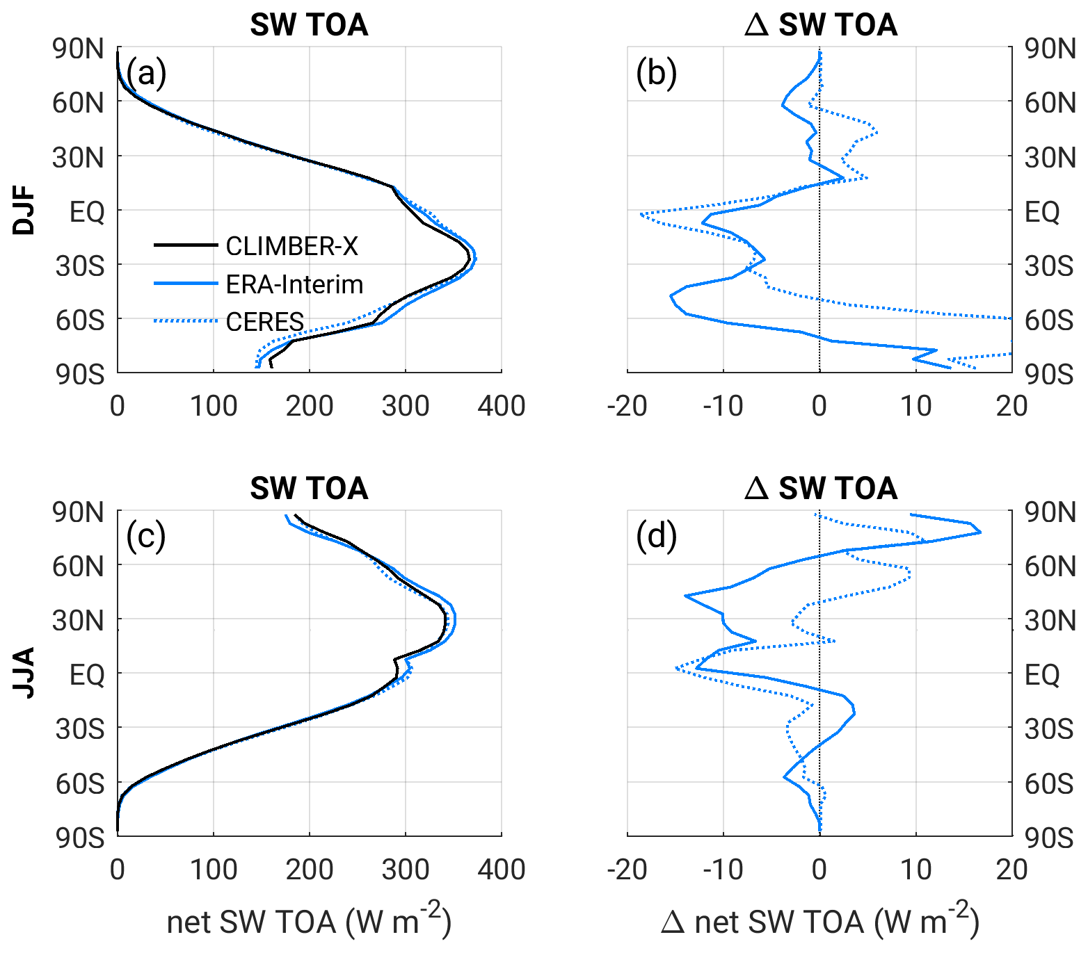
Figure A2 Zonal mean net shortwave radiation at the top of the atmosphere as computed by the CLIMBER-X radiation code in an offline set-up compared to ERA-Interim reanalysis (Dee et al., 2011) and CERES satellite observations (Loeb et al., 2018). Panels (a) and (b) are for December–January–February and panels (c) and (d) are for June–July–August. Panels (a) and (c) show absolute values, while panels (b) and (d) show model biases.

Figure A3 Shortwave radiative kernels at the top of the atmosphere for (a) a 1 % increase in surface albedo and (b) water vapour increase corresponding to a 1 K warming of the atmosphere. The kernels computed using the CLIMBER-X radiation code are compared to kernels available from different climate models (Shell et al., 2008; Block and Mauritsen, 2013; Smith et al., 2018; Pendergrass et al., 2018). Solid lines are for total-sky conditions, while dashed lines are for clear-sky conditions.

A8 Longwave radiation

Longwave radiative transfer follows in part from CLIMBER-2 as described in Petoukhov et al. (2003). Improvements relative to CLIMBER-2 include

• relaxing the assumption that clouds act as black bodies for longwave radiation, which is not strictly true for thin clouds in cold regions,

• a specific humidity profile derived from temperature and relative humidity, giving more consistent humidity/temperature values in the upper troposphere,

• CH₄, N₂O, CFC11 and CFC12 being considered through the use of an equivalent CO₂ concentration, and

• extensive retuning in an offline set-up using observations and output of atmospheric GCMs, including radiative kernels.

The computation of longwave radiative transfer is based on the two-stream approximation, where the downward and upward longwave radiative fluxes at any height z are computed as

$$\begin{array}{}\text{(A106)}& {\displaystyle }\begin{array}{rl}{F}_{\mathrm{LW}}^{\downarrow }\left(z\right)& =B\left(z\right)-B\left(H_{\mathrm{TOA}}\right)D(z,H_{\mathrm{TOA}})\\ & +\underset{z}{\overset{{\mathrm{H}}_{\mathrm{TOA}}}{\int }}D(z,z^{\prime }){\displaystyle \frac{\mathrm{d}B\left(z^{\prime }\right)}{\mathrm{d}{z}^{\prime }}}\mathrm{d}{z}^{\prime },\end{array}\text{(A107)}& {\displaystyle }\begin{array}{rl}{F}_{\mathrm{LW}}^{\uparrow }\left(z\right)& =B\left(z\right)+(B_{\mathrm{s}}-B(z_{\mathrm{s}}\left)\right)D(z_{\mathrm{s}},z)\\ & -\underset{{\mathrm{z}}_{\mathrm{s}}}{\overset{\mathrm{z}}{\int }}D(z,z^{\prime }){\displaystyle \frac{\mathrm{d}B\left(z^{\prime }\right)}{\mathrm{d}{z}^{\prime }}}\mathrm{d}{z}^{\prime },\end{array}\end{array}$$

where B(z)=σT⁴(z) is the longwave emission at height z, $B_{\mathrm{s}}=\mathit{ϵ}\mathit{\sigma }{T}_{\mathrm{s}}^{\mathrm{4}}$ the long wave emitted by the surface with an emissivity ϵ, σ the Stefan–Boltzmann constant, and $D(z,z^{\prime })$ the integral transmission function of the atmospheric layer confined between levels z and z^′. Longwave radiation fluxes are computed separately for clear sky and cloudy sky using the following integral transmission functions, which explicitly include the effect of water vapour, CO₂, O₃ and clouds:

$$\begin{array}{}\text{(A108)}& {\displaystyle }& {\displaystyle }{D}^{\mathrm{cs}}=D_{\mathrm{wv}}{D}_{{\mathrm{CO}}_{\mathrm{2}}}{D}_{{\mathrm{O}}_{\mathrm{3}}},\text{(A109)}& {\displaystyle }& {\displaystyle }{D}^{\mathrm{cld}}=D_{\mathrm{wv}}{D}_{{\mathrm{CO}}_{\mathrm{2}}}{D}_{{\mathrm{O}}_{\mathrm{3}}}{D}_{\mathrm{cld}}.\end{array}$$

The integral transmission functions for water vapour, CO₂, O₃ and clouds are given by

$$\begin{array}{}\text{(A110)}& {\displaystyle }\begin{array}{rl}{D}_{\mathrm{wv}}(z_{\mathrm{1}},z_{\mathrm{2}})& =\left(\mathrm{1}+a_{\mathrm{1}}^{\mathrm{wv}}\left({\mathit{\beta }}_{\mathrm{0}}{M}_{\mathrm{wv}}\right(z_{\mathrm{1}},z_{\mathrm{2}}){)}^{{\mathit{\beta }}_{\mathrm{1}}^{\mathrm{wv}}}\right.\\ & +a_{\mathrm{2}}^{\mathrm{wv}}\left({\mathit{\beta }}_{\mathrm{0}}{M}_{\mathrm{wv}}\right(z_{\mathrm{1}},z_{\mathrm{2}}){)}^{{\mathit{\beta }}_{\mathrm{2}}^{\mathrm{wv}}}\\ & {\left.+a_{\mathrm{3}}^{\mathrm{wv}}\left({\mathit{\beta }}_{\mathrm{0}}{M}_{\mathrm{wv}}\right(z_{\mathrm{1}},z_{\mathrm{2}}){)}^{{\mathit{\beta }}_{\mathrm{3}}^{\mathrm{wv}}}\right)}^{-\mathrm{1}},\end{array}\text{(A111)}& {\displaystyle }\begin{array}{rl}{D}_{{\mathrm{CO}}_{\mathrm{2}}}(z_{\mathrm{1}},z_{\mathrm{2}})& =\left(\mathrm{1}-\mathrm{0.1}{\left({\displaystyle \frac{M_{{\mathrm{CO}}_{\mathrm{2}}(z_{\mathrm{1}},z_{\mathrm{2}})}}{\mathrm{1000}}}\right)}^{\mathrm{2}}\right)\\ & \times {\displaystyle \frac{\mathrm{1}+a_{\mathrm{0}}^{{\mathrm{CO}}_{\mathrm{2}}}{a}_{\mathrm{1}}^{{\mathrm{CO}}_{\mathrm{2}}}\left({\mathit{\beta }}_{\mathrm{0}}{M}_{{\mathrm{CO}}_{\mathrm{2}}}\right(z_{\mathrm{1}},z_{\mathrm{2}}){)}^{{\mathit{\beta }}_{\mathrm{1}}^{{\mathrm{CO}}_{\mathrm{2}}}}}{\mathrm{1}+a_{\mathrm{0}}^{{\mathrm{CO}}_{\mathrm{2}}}\left({\mathit{\beta }}_{\mathrm{0}}{M}_{{\mathrm{CO}}_{\mathrm{2}}}\right(z_{\mathrm{1}},z_{\mathrm{2}}){)}^{{\mathit{\beta }}_{\mathrm{2}}^{{\mathrm{CO}}_{\mathrm{2}}}}}},\end{array}\text{(A112)}& {\displaystyle }{D}_{{\mathrm{O}}_{\mathrm{3}}}(z_{\mathrm{1}},z_{\mathrm{2}})=\mathrm{1}-a^{{\mathrm{O}}_{\mathrm{3}}}\left(M_{{\mathrm{O}}_{\mathrm{3}}}\right(z_{\mathrm{1}},z_{\mathrm{2}}){)}^{{\mathit{\beta }}^{{\mathrm{O}}_{\mathrm{3}}}},\text{(A113)}& {\displaystyle }\begin{array}{rl}{D}_{\mathrm{cld}}(z_{\mathrm{1}},z_{\mathrm{2}})& =\exp \left(-{\displaystyle \frac{|z-z^{\prime }|}{H_{\mathrm{cld}}^{\mathrm{top}}-H_{\mathrm{cld}}^{\mathrm{base}}}}{\mathit{\tau }}_{\mathrm{cld}}\right)\\ & \text{only inside cloud layers}.\end{array}\end{array}$$

The first term on the right-hand side of Eq. (A111) ensures that the radiative forcing of CO₂ increases with increasing CO₂, in accordance with Hansen (2005) and Colman and McAvaney (2009). The effective absorber mass of water vapour, CO₂ and O₃ is computed from

$$\begin{array}{}\text{(A114)}& {\displaystyle }& {\displaystyle }{M}_{\mathrm{wv}}(z_{\mathrm{1}},z_{\mathrm{2}})=\underset{z_{\mathrm{1}}}{\overset{z_{\mathrm{2}}}{\int }}q\left(z\right)\mathit{\rho }\left(z\right){\left({\displaystyle \frac{p\left(z\right)}{p\left(\mathrm{0}\right)}}\right)}^{k_{\mathrm{wv}}}\mathrm{d}z,\text{(A115)}& {\displaystyle }& {\displaystyle }{M}_{{\mathrm{CO}}_{\mathrm{2}}}(z_{\mathrm{1}},z_{\mathrm{2}})={\mathrm{CO}}_{\mathrm{2}}\underset{z_{\mathrm{1}}}{\overset{z_{\mathrm{2}}}{\int }}\mathit{\rho }\left(z\right){\left({\displaystyle \frac{p\left(z\right)}{p\left(\mathrm{0}\right)}}\right)}^{k_{{\mathrm{CO}}_{\mathrm{2}}}}\mathrm{d}z,\text{(A116)}& {\displaystyle }& {\displaystyle }{M}_{{\mathrm{O}}_{\mathrm{3}}}(z_{\mathrm{1}},z_{\mathrm{2}})=\underset{z_{\mathrm{1}}}{\overset{z_{\mathrm{2}}}{\int }}{\mathrm{O}}_{\mathrm{3}}\left(z\right)\mathit{\rho }\left(z\right){\left({\displaystyle \frac{p\left(z\right)}{p\left(\mathrm{0}\right)}}\right)}^{k_{{\mathrm{O}}_{\mathrm{3}}}}\mathrm{d}z.\end{array}$$

The effect of the well-mixed greenhouse gases CH₄, N₂O and CFCs on longwave radiation is accounted for through a CO₂ equivalent following Etminan et al. (2016):

$$\begin{array}{}\text{(A117)}& \begin{array}{rl}& {\mathrm{CO}}_{\mathrm{2}}^{\mathrm{eq}}={{\mathrm{CO}}_{\mathrm{2}}}^{\mathrm{0}}\exp \\ & \left({\displaystyle \frac{R\left({\mathrm{CO}}_{\mathrm{2}}\right)+R\left({\mathrm{CH}}_{\mathrm{4}}\right)+R\left({\mathrm{N}}_{\mathrm{2}}\mathrm{O}\right)+R\left(\mathrm{CFC}\mathrm{11}\right)+R\left(\mathrm{CFC}\mathrm{12}\right)}{a_{\mathrm{1}}{\left({\mathrm{CO}}_{\mathrm{2}}-{{\mathrm{CO}}_{\mathrm{2}}}^{\mathrm{0}}\right)}^{\mathrm{2}}+b_{\mathrm{1}}\left|{\mathrm{CO}}_{\mathrm{2}}-{{\mathrm{CO}}_{\mathrm{2}}}^{\mathrm{0}}\right|+c_{\mathrm{1}}\stackrel{\mathrm{‾}}{{\mathrm{N}}_{\mathrm{2}}\mathrm{O}}+\mathrm{5.36}}}\right)\end{array}\end{array}$$

The radiative forcing R of CO₂, CH₄ and N₂O is computed as in Table 1 of Etminan et al. (2016) and the radiative forcing of CFC11 and CFC12 as in Table 3 of Myhre et al. (1998).

Similarly to shortwave radiation, longwave radiation is computed for each macro surface type individually. Atmospheric characteristics for each type within a given grid cell are the same but surface elevation and surface temperature are different. By default, for longwave radiation the atmosphere is divided into 15 vertical levels: 6 between surface and base of clouds, 3 between the base and top of clouds, 3 between the top of clouds and the tropopause and 3 in the stratosphere. Total longwave radiation fluxes in each grid cell are taken as cloud fraction weighted sum of clear sky and cloudy sky fluxes.

Longwave radiation parameters (in particular those related to the integral transmission functions) are tuned in offline mode using prescribed 3-D temperature and water vapour fields and cloud cover fraction from ERA-Interim reanalysis (Dee et al., 2011), cloud top height and cloud optical thickness from the ISCCP climatology Rossow and Schiffer (1999), and O₃ concentration from historical simulations of selected CMIP6 models. The target is to minimize the root mean square error in top-of-the-atmosphere and surface longwave radiation fluxes for clear sky and total sky. The resulting zonal mean net top-of-the-atmosphere longwave radiation is shown in Figs. A4 and A5, for clear-sky and total sky, respectively. Additional constraints on model parameters are provided by the longwave radiative kernels at the TOA and at the surface, which are available for several climate models (Shell et al., 2008; Block and Mauritsen, 2013; Smith et al., 2018; Pendergrass et al., 2018). The TOA kernels computed using the CLIMBER-X longwave radiation code are compared to those available from the different climate models in Fig. A6, demonstrating that the simplified longwave radiation scheme employed in CLIMBER-X also represents well the sensitivities of longwave radiation fluxes to changes in temperature, humidity and CO₂. The total greenhouse effect separation presented in Schmidt et al. (2010) is used as a further constraint on longwave radiation parameters. The effect of removing different longwave absorbers on the net longwave radiation at TOA is computed and compared to the values of Schmidt et al. (2010) in Table A8.

Table A7 Longwave radiation parameters.

Schmidt et al. (2010)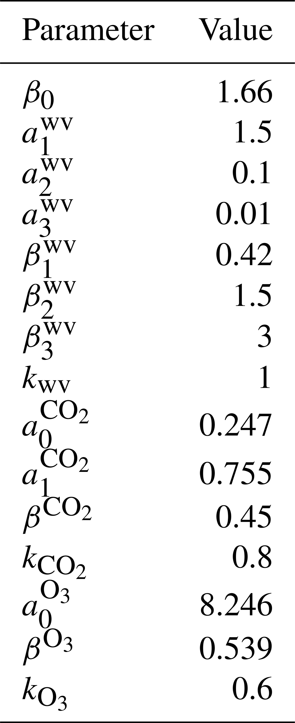

Table A8 Effect of removing different longwave absorbers on the net longwave absorbed by the circa 1980 atmosphere. The unit is W m⁻². The reference values are from Schmidt et al. (2010).

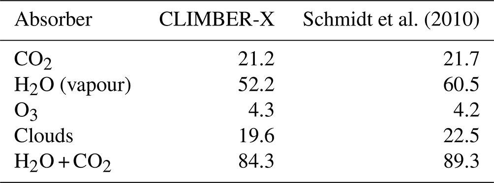
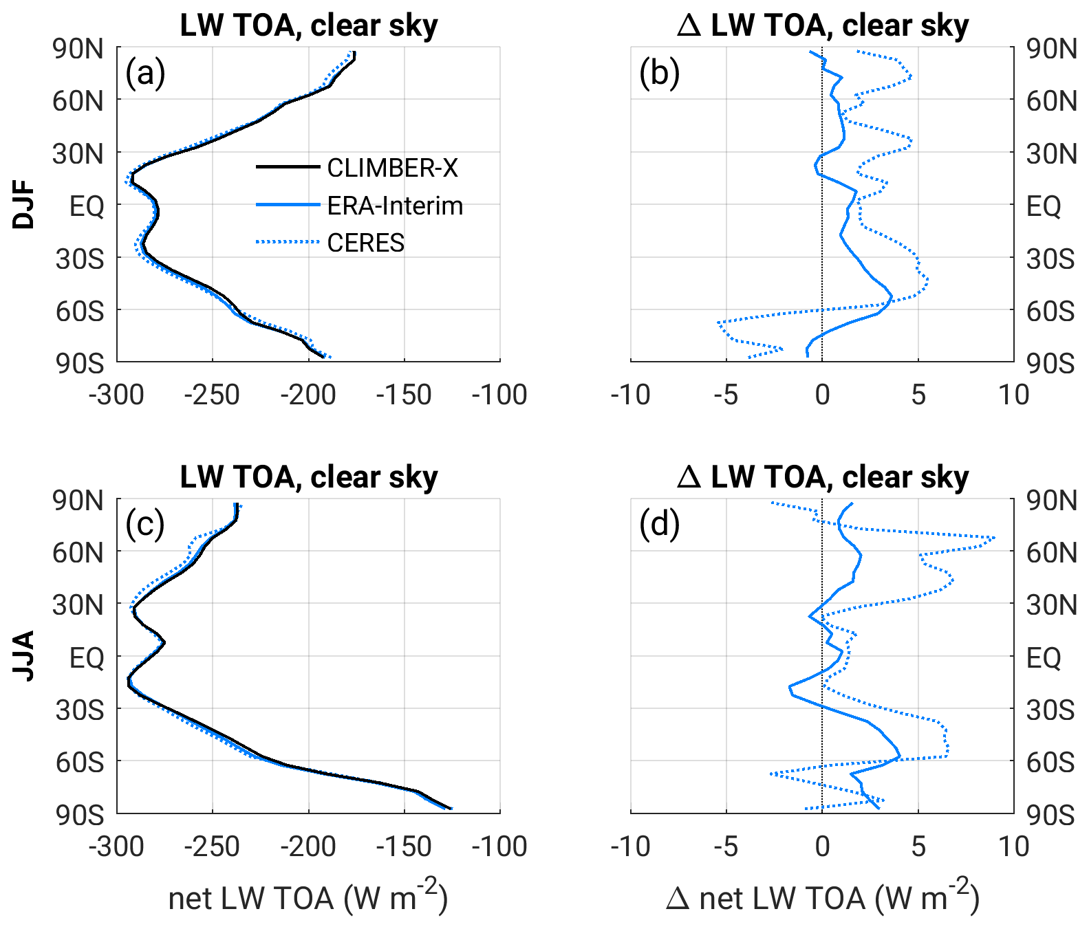
Figure A4 Zonal mean net longwave radiation at the top of the atmosphere for clear-sky conditions as computed by the CLIMBER-X radiation code in an offline set-up compared to ERA-Interim reanalysis (Dee et al., 2011) and CERES satellite observations (Loeb et al., 2018). Panels (a) and (b) are for December–January–February and panels (c) and (d) are for June–July–August. Panels (a) and (c) show absolute values, while panels (b) and (d) show model biases.

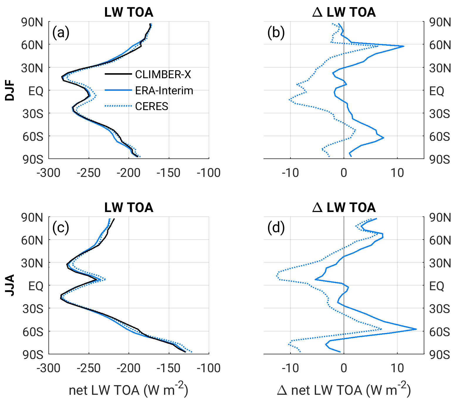
Figure A5 Zonal mean net longwave radiation at the top of the atmosphere as computed by the CLIMBER-X radiation code in an offline set-up compared to ERA-Interim reanalysis (Dee et al., 2011) and CERES satellite observations (Loeb et al., 2018). Panels (a) and (b) are for December–January–February and panels (c) and (d) are for June–July–August. Panels (a) and (c) show absolute values, while panels (b) and (d) show model biases.

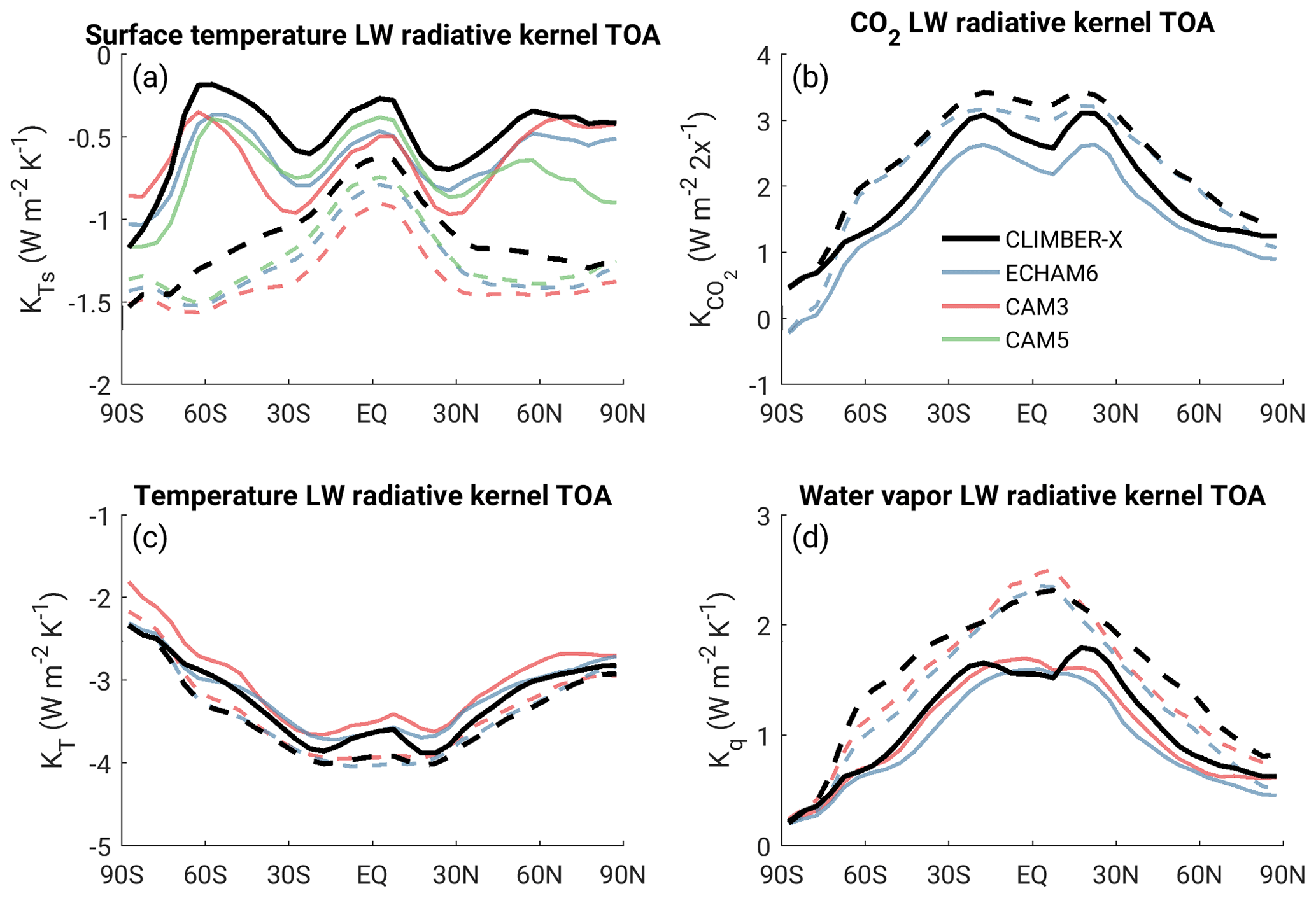
Figure A6 Longwave radiative kernels at the top of the atmosphere for (a) surface temperature warming by 1 K, (b) atmospheric CO₂ doubling, (c) air temperature warming by 1 K and (d) water vapour increase corresponding to 1 K warming in the atmosphere. The kernels computed using the CLIMBER-X radiation code are compared to kernels available from different climate models (Shell et al., 2008; Block and Mauritsen, 2013; Pendergrass et al., 2018). Solid lines are for total-sky conditions, while dashed lines are for clear-sky conditions.

Appendix B: GOLDSTEIN detailed description

The horizontal ocean velocity in GOLDSTEIN is diagnosed from a frictional–geostrophic balance:

$$\begin{array}{}\text{(B1)}& {\displaystyle }-fv+\mathit{\mu }u-{\displaystyle \frac{\mathrm{1}}{{\mathit{\rho }}_{\mathrm{0}}}}{\displaystyle \frac{\partial {\mathit{\tau }}_{\mathit{\lambda }}}{\partial z}}& {\displaystyle }=-{\displaystyle \frac{\mathrm{1}}{{\mathit{\rho }}_{\mathrm{0}}{R}_{\mathrm{e}}\cos \mathit{\varphi }}}{\displaystyle \frac{\partial p}{\partial \mathit{\lambda }}}\text{(B2)}& {\displaystyle }fu+\mathit{\mu }v-{\displaystyle \frac{\mathrm{1}}{{\mathit{\rho }}_{\mathrm{0}}}}{\displaystyle \frac{\partial {\mathit{\tau }}_{\mathit{\varphi }}}{\partial z}}& {\displaystyle }=-{\displaystyle \frac{\mathrm{1}}{{\mathit{\rho }}_{\mathrm{0}}{R}_{\mathrm{e}}}}{\displaystyle \frac{\partial p}{\partial \mathit{\varphi }}},\end{array}$$

The drag coefficient μ is composed of a uniform background value μ₀, which, for barotropic velocities, is enhanced by a factor of 3 in waters shallower than 1000 m. The definition of the wind or sea ice stress τ is given in Appendix A5 above. Hydrostatic balance is assumed:

$$\begin{array}{}\text{(B3)}& {\displaystyle \frac{\partial p}{\partial z}}=-g\mathit{\rho }(\mathit{\theta },S,p_{\mathrm{0}}(z\left)\right),\end{array}$$

where $p_{\mathrm{0}}\left(z\right)=\mathrm{0.1}\cdot z$. Seawater density, $\mathit{\rho }(\mathit{\theta },S,p_{\mathrm{0}}(z\left)\right)$, is computed using the UNESCO equation of state of Millero and Poisson (1981) with the bulk secant modulus expressed in terms of potential temperature using the coefficients of Jackett and McDougall (1995). For computational efficiency only 7 of the originally 26 terms are kept in the bulk secant modulus polynomial. A comparison between the full equation of state of Jackett and McDougall (1995) and the truncated version showed negligible differences in the simulated ocean state. The vertical velocity is then derived from the continuity equation:

$$\begin{array}{}\text{(B4)}& \mathrm{\nabla }\cdot \mathit{u}=\mathrm{0}.\end{array}$$

Equations (B1) through (B4) are solved by separation of the velocity into a barotropic and a baroclinic component, as described in detail in Edwards et al. (1998) and Müller et al. (2006). More details on the treatment of barotropic flow around islands are given in Edwards and Shepherd (2002).

The transport equation for tracers takes the following form:

$$\begin{array}{}\text{(B5)}& {\displaystyle \frac{\partial X}{\partial t}}+\mathrm{\nabla }\cdot \left(\mathit{u}X\right)=\mathrm{\nabla }\left(\mathit{A}\mathrm{\nabla }X\right)+\mathrm{SMS}.\end{array}$$

X is the tracer concentration, SMS represents source minus sinks and A is the diffusive mixing tensor:

$$\begin{array}{}\text{(B6)}& A=\left(\begin{array}{rrr}{K}_{\mathrm{I}}& \mathrm{0}& (K_{\mathrm{I}}-\mathit{\kappa })S_{\mathit{\lambda }}\\ \mathrm{0}& K_{\mathrm{I}}& (K_{\mathrm{I}}-\mathit{\kappa })S_{\mathit{\varphi }}\\ (K_{\mathrm{I}}+\mathit{\kappa })S_{\mathit{\lambda }}& (K_{\mathrm{I}}+\mathit{\kappa })S_{\mathit{\varphi }}& K_{\mathrm{I}}{\mathit{S}}^{\mathrm{2}}+K_{\mathrm{D}}\end{array}\right),\end{array}$$

with K_I and K_D the isopycnal and diapycnal diffusivities, respectively, κ the Gent–McWilliams parameter which parameterizes sub-scale eddies and the slope of the isopycnals is:

$$\begin{array}{}\text{(B7)}& \mathit{S}=\left(S_{\mathit{\lambda }},S_{\mathit{\varphi }},\mathrm{0}\right)=\left(-{\displaystyle \frac{\frac{\mathrm{1}}{R_{\mathrm{e}}\cos \mathit{\varphi }}\frac{\partial \mathit{\rho }}{\partial \mathit{\lambda }}}{\frac{\partial \mathit{\rho }}{\partial z}}},-{\displaystyle \frac{\frac{\mathrm{1}}{R_{\mathrm{e}}}\frac{\partial \mathit{\rho }}{\partial \mathit{\varphi }}}{\frac{\partial \mathit{\rho }}{\partial z}}},\mathrm{0}\right).\end{array}$$

Diapycnal diffusivity is a prescribed function of depth:

$$\begin{array}{}\text{(B8)}& \begin{array}{rl}{K}_{\mathrm{D}}& =K_{\mathrm{D}}^{\min }+{\displaystyle \frac{\arctan \left(\frac{z-z_{\mathrm{ref}}}{\mathrm{1000}}\right)-\arctan \left(\frac{-z_{\mathrm{ref}}}{\mathrm{1000}}\right)}{\arctan \left(\frac{\mathrm{5000}-z_{\mathrm{ref}}}{\mathrm{1000}}\right)-\arctan \left(\frac{-z_{\mathrm{ref}}}{\mathrm{1000}}\right)}}\\ & \cdot \left(K_{\mathrm{D}}^{\max }-K_{\mathrm{D}}^{\min }\right).\end{array}\end{array}$$

If the stratification of a water column is statically unstable, convective adjustment is applied using the scheme of Rahmstorf (1993). A simple mixed-layer scheme based on Kraus and Turner (1967) is used in the model.

The equations are discretized on a staggered Arakawa C grid.

Table B1 Ocean model parameters.

Appendix C: SISIM detailed description

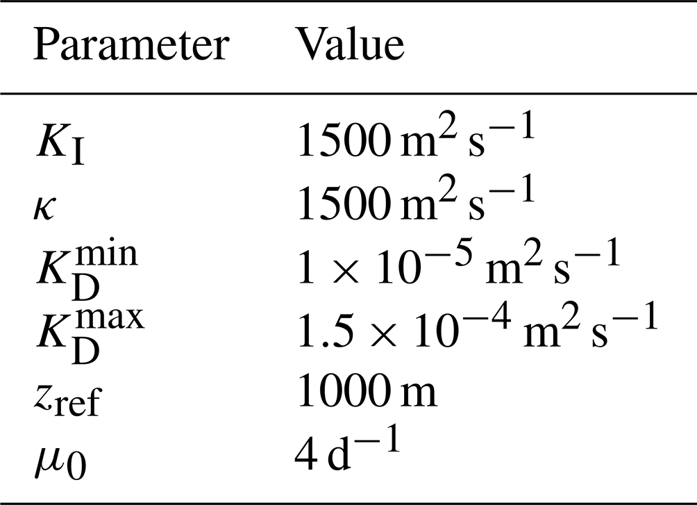
Sea ice thermodynamics is based on the zero-layer model of Semtner (1976). The surface energy fluxes are computed separately over sea ice and over open ocean. Over sea ice, the surface energy balance equation is written as

$$\begin{array}{}\text{(C1)}& (\mathrm{1}-\mathit{\alpha }){\mathrm{SW}}^{\downarrow }+\mathit{ϵ}{\mathrm{LW}}^{\downarrow }-{\mathrm{LW}}^{\uparrow }-\mathrm{SH}-\mathrm{LE}-G=\mathrm{0},\end{array}$$

where α is surface albedo, SW^↓ is the incoming shortwave radiation, ϵ is the surface emissivity for longwave radiation, LW^↓ and LW^↑ are the incoming and outgoing longwave radiation at the surface, SH is the sensible heat flux, LE is the latent heat flux and G the heat flux into the snow/ice. Equation (C1) is then solved for the skin temperature, T_⋆, using the formulations for the energy fluxes described next. Bare sea ice albedo is temperature-dependent following

$$\begin{array}{}\text{(C2)}& {\displaystyle }& {\displaystyle }{\mathit{\alpha }}_{\mathrm{vu}}=\mathrm{0.8}-\mathrm{0.075}\left(T_{\star }-T_{\mathrm{0}}+\mathrm{1}\right),\text{(C3)}& {\displaystyle }& {\displaystyle }{\mathit{\alpha }}_{\mathrm{ir}}=\mathrm{0.6}-\mathrm{0.075}\left(T_{\star }-T_{\mathrm{0}}+\mathrm{1}\right).\end{array}$$

The snow albedo scheme is the same as used in the land model and includes a dependence on snow grain size and dust and soot concentration following Dang et al. (2015). The fraction of sea ice covered by snow is computed from snow thickness as

$$\begin{array}{}\text{(C4)}& f_{\mathrm{snow}}={\displaystyle \frac{h_{\mathrm{snow}}}{h_{\mathrm{snow}}+\mathrm{0.02}}}.\end{array}$$

The surface emitted longwave radiation is given by the Stefan–Boltzmann law:

$$\begin{array}{}\text{(C5)}& {\mathrm{LW}}^{\uparrow }=\mathit{ϵ}\mathit{\sigma }{T}_{\star }^{\mathrm{4}}.\end{array}$$

The sensible heat flux is computed from the temperature gradient between the skin and near-surface air, using the bulk aerodynamic formula:

$$\begin{array}{}\text{(C6)}& \mathrm{SH}={\displaystyle \frac{{\mathit{\rho }}_{\mathrm{a}}{c}_{\mathrm{p}}}{r_{\mathrm{aer}}}}(T_{\star }-T_{\mathrm{2}\mathrm{m}}),\end{array}$$

where ρ_a is air density, c_p is the specific heat of air, r_aer is the aerodynamic resistance and T_2 m is the near-surface air temperature. Similarly, the latent heat flux over sea ice is expressed in terms of the specific humidity gradient between the surface and near-surface air:

$$\begin{array}{}\text{(C7)}& \mathrm{LE}=L{\displaystyle \frac{{\mathit{\rho }}_{\mathrm{a}}}{r_{\mathrm{aer}}}}\left(q_{\mathrm{sat}}\left(T_{\star }\right)-q_{\mathrm{2}\mathrm{m}}\right).\end{array}$$

L is the latent heat of sublimation, q_sat is the specific humidity at saturation and q_2 m is the specific humidity of near-surface air. The aerodynamic resistance is computed from wind speed, surface exchange coefficient and bulk Richardson number following Willeit and Ganopolski (2016).

The conductive heat flux into the snow/ice (G) is computed as

$$\begin{array}{}\text{(C8)}& G={\mathit{\lambda }}_{\mathrm{eff}}\left(T_{\star }-T_{\mathrm{f}}\right),\end{array}$$

where T_f is the salinity-dependent freezing temperature at the base of the ice (Millero and Poisson, 1981):

$$\begin{array}{}\text{(C9)}& T_{\mathrm{f}}=-\mathrm{0.0575}\cdot S_{\mathrm{o}}+\mathrm{0.0017}\cdot S_{\mathrm{o}}^{\mathrm{1.5}}-\mathrm{0.0002}\cdot S_{\mathrm{o}}^{\mathrm{2}}+T_{\mathrm{0}}\end{array}$$

and the effective snow/ice heat conductivity is

$$\begin{array}{}\text{(C10)}& {\mathit{\lambda }}_{\mathrm{eff}}=k_{\mathit{\lambda }}{\displaystyle \frac{{\mathit{\lambda }}_{\mathrm{snow}}\cdot }{h_{\mathrm{snow}}+\left(h_{\mathrm{ice}}\right){\mathit{\lambda }}_{\mathrm{snow}}/{\mathit{\lambda }}_{\mathrm{ice}}}}.\end{array}$$

The k_λ factor accounts for sub-grid ice thickness distribution following Eq. (2) in (Fichefet and Maqueda, 1997). The prognostic terms in T_⋆ in the formulation of the surface energy fluxes are then linearized using Taylor series expansion assuming that the temperature at the new time step, $T_{\star ,n+\mathrm{1}}=T_{\star ,n}+\mathrm{\Delta }T$ with $\mathrm{\Delta }{T}_{\star }\ll T_{\star }$:

$$\begin{array}{}\text{(C11)}& {\displaystyle }{T}_{\star ,n+\mathrm{1}}^{\mathrm{4}}=T_{\star ,n}^{\mathrm{4}}+\mathrm{4}{T}_{\star ,n}^{\mathrm{3}}(T_{\star ,n+\mathrm{1}}-T_{\star ,n}),\text{(C12)}& {\displaystyle }{q}_{\mathrm{sat}}\left(T_{\star ,n+\mathrm{1}}\right)=q_{\mathrm{sat}}\left(T_{\star }\right)+{\displaystyle \frac{\mathrm{d}{q}_{\mathrm{sat}}}{\mathrm{d}{T}_{\star }}}{|}_{T_{\star }=T_{\star ,n}}(T_{\star ,n+\mathrm{1}}-T_{\star ,n}).\end{array}$$

Equation (C1) can then be solved explicitly for the skin temperature at the new time step, $T_{\star ,n+\mathrm{1}}$. If the skin temperature is above freezing the surface energy fluxes are diagnosed first with the skin temperature greater then 0 ^∘C and then with skin temperature set to 0 ^∘C. The difference between the sum of the energy fluxes is then used to melt snow and/or ice.

Whether bottom ice accretion or ablation occurs depends on the sign of the net energy flux at the ice–water interface, which is determined by the balance between the conductive heat flux through the snow/ice layer (G) and the turbulent heat flux between the ice and the seawater below (McPhee, 1992; Weaver et al., 2001):

$$\begin{array}{}\text{(C13)}& H=C_{\mathrm{h}}{u}_{\star }{\mathit{\rho }}_{\mathrm{w}}{c}_{\mathrm{w}}\cdot \left(T_{\mathrm{f}}-T_{\mathrm{o}}\right).\end{array}$$

C_h is a constant exchange coefficient, u_⋆ the (constant) friction velocity, ρ_w water density and c_w the specific heat capacity of water.

Over seawater, the heat flux into the ocean is derived as the residual of the radiation and surface energy fluxes, which are computed similarly to the surface energy fluxes over sea ice, but using sea surface temperature instead of skin temperature. The albedo of seawater for diffuse radiation is 0.06, while the clear-sky albedo includes a dependence on the cosine of the solar zenith angle (μ):

$$\begin{array}{}\text{(C14)}& \mathit{\alpha }=min\left(\mathrm{0.2},{\displaystyle \frac{\mathrm{0.03}}{\mathit{\mu }}}\right).\end{array}$$

The longwave emissivity of water is set to 0.98. Sea ice in leads forms whenever the top-layer ocean temperature drops below the freezing point of seawater.

Table C1 Sea ice model parameters.

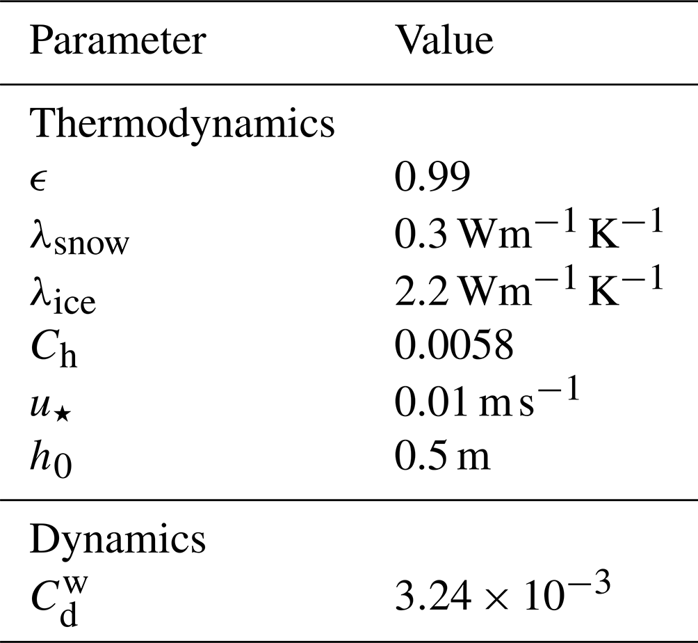
Sub-grid-scale thermodynamic processes of sea ice growth and melt are assumed to affect the sea ice concentration (f_ice) within a grid cell following Marsland et al. (2003) and Fichefet and Maqueda (1997):

$$\begin{array}{}\text{(C15)}& {\displaystyle \frac{\partial f_{\mathrm{ice}}}{\partial t}}=\mathrm{\Delta }{f}_{\mathrm{ice}}{|}_{\mathrm{frz}}+\mathrm{\Delta }{f}_{\mathrm{ice}}{|}_{\mathrm{melt}}.\end{array}$$

When freezing occurs over open water the sea ice concentration increases at a rate given by

$$\begin{array}{}\text{(C16)}& \mathrm{\Delta }{f}_{\mathrm{ice}}{|}_{\mathrm{frz}}=\sqrt{\mathrm{1}-f_{\mathrm{ice}}^{\mathrm{2}}}\cdot \left(\mathrm{1}-f_{\mathrm{ice}}\right){\displaystyle \frac{\mathrm{\Delta }{h}_{\mathrm{ice}}{|}_{\mathrm{frz}}}{h_{\mathrm{0}}}},\end{array}$$

where Δh_ice|_frz is the thickness of new sea ice formed and h₀ is an arbitrary demarcation thickness. Melting of sea ice results in a decrease in sea ice concentration:

$$\begin{array}{}\text{(C17)}& \mathrm{\Delta }{f}_{\mathrm{ice}}{|}_{\mathrm{melt}}=f_{\mathrm{ice}}{\displaystyle \frac{\mathrm{\Delta }{h}_{\mathrm{ice}}{|}_{\mathrm{melt}}}{\mathrm{2}{h}_{\mathrm{ice}}}},\end{array}$$

where Δh_ice|_melt is the change in sea ice thickness due to melting. This formulation is based on the assumption that sea ice thickness within a grid cell has a uniform distribution between 0 and 2h_ice.

Sea ice drift velocities are computed from the momentum balance equation (e.g. Hibler, 1979):

$$\begin{array}{}\text{(C18)}& m{\displaystyle \frac{\partial {\mathit{u}}_{\mathrm{i}}}{\partial t}}=\mathrm{\nabla }\cdot \mathit{\sigma }+{\mathit{\tau }}_{\mathrm{a}}+{\mathit{\tau }}_{\mathrm{o}}-\widehat{\mathit{k}}\times mf{\mathit{u}}_{\mathrm{i}}-mg\mathrm{\nabla }{H}_{\mathrm{o}},\end{array}$$

where ${\mathit{u}}_{\mathrm{i}}=\left(u_{\mathrm{i}},v_{\mathrm{i}}\right)$ is the sea ice velocity vector, m is the mass of ice and snow per unit area, f is the Coriolis parameter, H_o is the sea surface height and τ_a and τ_o are the wind and ocean stresses, respectively. The mechanical properties of the ice are represented by the internal stress tensor σ, and the elastic–viscous–plastic rheology of Hunke and Dukowicz (1997); Bouillon et al. (2009) is used as a constitutive law relating the internal stress to the strain rate. The numerical solution follows the implementation in the GFDL model SIS2 (Adcroft et al., 2019; Delworth et al., 2006). The sea surface height is diagnosed to a first approximation from the seawater density above a reference depth of 1500 m. The zonal and meridional components of the wind stress on sea ice are computed as

$$\begin{array}{}\text{(C19)}& {\displaystyle }& {\displaystyle }{\mathit{\tau }}_{\mathrm{a}}^{\mathrm{u}}=C_{\mathrm{d}}{\mathit{\rho }}_{\mathrm{a}}{u}_{\mathrm{s}}{U}_{\mathrm{s}},\text{(C20)}& {\displaystyle }& {\displaystyle }{\mathit{\tau }}_{\mathrm{a}}^{\mathrm{v}}=C_{\mathrm{d}}{\mathit{\rho }}_{\mathrm{a}}{v}_{\mathrm{s}}{U}_{\mathrm{s}},\end{array}$$

with the symbols defined in Appendix A2 above. The components of the stress exerted by the ocean on sea ice are given by

$$\begin{array}{}\text{(C21)}& {\displaystyle }& {\displaystyle }{\mathit{\tau }}_{\mathrm{o}}^{\mathrm{u}}=C_{\mathrm{d}}^{\mathrm{w}}{\mathit{\rho }}_{\mathrm{w}}\sqrt{{\left(u_{\mathrm{i}}-u_{\mathrm{o}}\right)}^{\mathrm{2}}+{\left(v_{\mathrm{i}}-v_{\mathrm{o}}\right)}^{\mathrm{2}}}\cdot \left(u_{\mathrm{i}}-u_{\mathrm{o}}\right),\text{(C22)}& {\displaystyle }& {\displaystyle }{\mathit{\tau }}_{\mathrm{o}}^{\mathrm{v}}=C_{\mathrm{d}}^{\mathrm{w}}{\mathit{\rho }}_{\mathrm{w}}\sqrt{{\left(u_{\mathrm{i}}-u_{\mathrm{o}}\right)}^{\mathrm{2}}+{\left(v_{\mathrm{i}}-v_{\mathrm{o}}\right)}^{\mathrm{2}}}\cdot \left(v_{\mathrm{i}}-v_{\mathrm{o}}\right),\end{array}$$

where $C_{\mathrm{d}}^{\mathrm{w}}$ is the drag coefficient between the sea ice and water and (u_o,v_o) the top-layer ocean velocity. The derived sea ice velocities are then used to advect the grid cell mean ice and snow thicknesses and the sea ice concentration using a flux-corrected transport scheme (Zalesak, 1979). No explicit diffusion is applied.

Appendix D: PALADYN surface albedo

Several changes to the surface albedo scheme have been introduced into the model compared to the description in Willeit and Ganopolski (2016).

The parameterization of sub-grid snow cover fraction has been updated considering also the effect of topographic roughness following Niu and Yang (2007) and Roesch et al. (2001):

$$\begin{array}{}\text{(D1)}& f_{\mathrm{sn}}=\tanh \left({\displaystyle \frac{h_{\mathrm{sn}}}{\mathrm{10}\cdot z_{\mathrm{0}}}}\right){\displaystyle \frac{h_{\mathrm{sn}}}{h_{\mathrm{sn}}+\mathrm{1}\times {\mathrm{10}}^{-\mathrm{4}}\cdot {\mathit{\sigma }}_{\mathrm{oro}}}},\end{array}$$

where h_sn is snow thickness, z₀ is the surface roughness length and σ_oro is the sub-grid standard deviation of the orography.

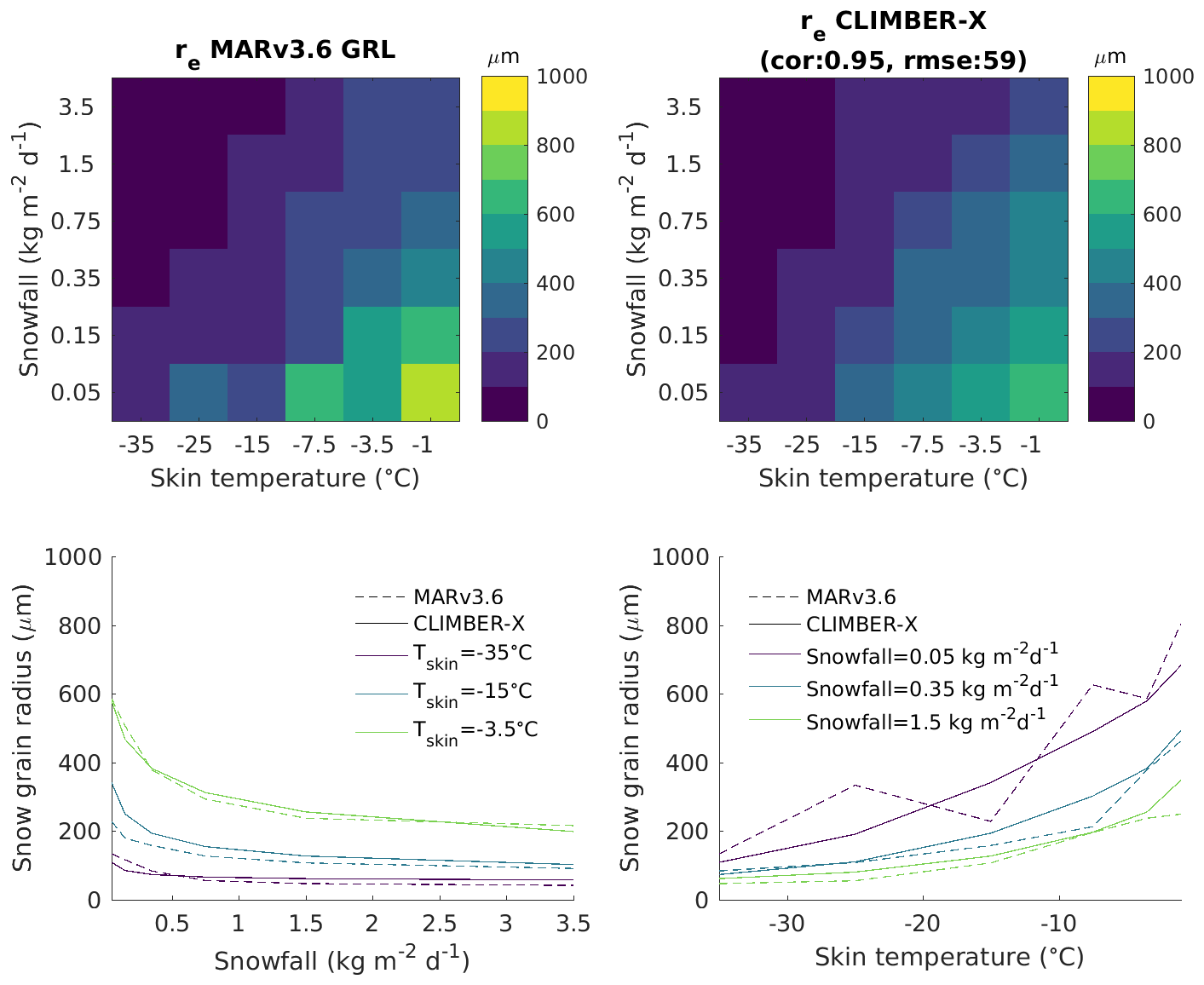
Figure D1 Snow grain size parameterization as a function of skin temperature and snowfall rate.

The snow albedo scheme has been refined with the inclusion of the effect of dust and soot on snow albedo following Dang et al. (2015) and the snow grain size parameterization has been retuned using output of the regional climate model MARv3.6 simulations for Greenland (Fettweis et al., 2017). The resulting dependence of snow grain size on climatological values of skin temperature and snowfall rate are shown in Fig. D1.