the Creative Commons Attribution 4.0 License.
the Creative Commons Attribution 4.0 License.
 | 21 Jul 2022
LAND-SUITE V1.0: a suite of tools for statistically based landslide susceptibility zonation
Txomin Bornaetxea
Paola Reichenbach
In the past 50 years, a large variety of statistically based models and methods for landslide susceptibility mapping and zonation have been proposed in the literature. The methods, which are applicable to a large range of spatial scales, use a large variety of input thematic data, different model combinations, and several approaches to evaluate the models' performance. Despite the numerous applications available in the literature, a standard approach for susceptibility modeling and zonation is still missing.
The literature search revealed that several software program and tools are available to evaluate regional slope stability using physically based analysis, but only a few use statistically based approaches. Among them, LAND-SE (LANDslide Susceptibility Evaluation) provides the possibility to perform and combine different statistical susceptibility models and to evaluate their performances and associated uncertainties. This paper describes the structure and the functionalities of LAND-SUITE, a suite of tools for statistically based landslide susceptibility modeling which integrates LAND-SE. LAND-SUITE completes and extends LAND-SE, adding functionalities to (i) facilitate input data preparation, (ii) perform preliminary and exploratory analysis of the available data, and (iii) test different combinations of variables and select the optimal thematic/explanatory set. LAND-SUITE provides a tool to assist the user during the data preparatory phase and to perform diversified statistically based landslide susceptibility applications.
- Article
(8861 KB) - Full-text XML
-
Supplement
(1627 KB) - BibTeX
- EndNote


Landslide susceptibility measures the degree to which a terrain can be affected by future slope movements and provides an estimate of where landslides are likely to occur (Chacon et al., 2006; Guzzetti et al., 2005). A wide variety of statistically based models and methods for landslide susceptibility mapping and zonation have been proposed in the literature in the past 50 years (Aleotti and Chowdhury, 1999; Huabin et al., 2005; Chacón et al., 2006; Fell et al., 2008; van Westen et al., 2008; Kanungo et al., 2012; Pardeshi et al., 2013; Reichenbach et al., 2018). Statistically based susceptibility models are applied to identify the functional (statistical) relationship between instability factors described by sets of geo-environmental (independent) variables and the known distribution of landslides, which is taken as the dependent model variable. This functional relationship is used to ascertain the propensity of the terrain to generate landslides and to predict susceptibility.
A recent review article published by Reichenbach et al. (2018) has shown that more than 163 model type names are listed in the literature by different authors. The models were classified into 19 groups that allowed highlighting the fact that logistic regression, neural networks, and data overlay model are the most often used modeling approaches. The literature review also revealed a considerable variability of landslide and thematic data types, scales selected for the modeling, and diversified choice of criteria used to evaluate the model performances. All these different issues, as well as their possible combinations, suggest that it is possible to select and apply a vast and heterogeneous number of methodologies to assess landslide susceptibility. As a matter of fact, a standardized methodology, procedure, and software for susceptibility assessment are still missing.
As an attempt to fill this gap, Reichenbach et al. (2018) suggest nine interrelated steps to prepare a reliable landslide susceptibility assessment and for the proper use of the associated terrain zonations (see Table 3 in Reichenbach et al., 2018). Such a methodological guideline allows for proceduralized but flexible susceptibility assessments, although it assumes basic expertise and skills in geomorphology, data preparation, data analysis, and geo-computation.
In the literature, several articles describe tools suitable for the analysis of shallow landslides using physically based slope stability simulators (for example, SHALSTAB by Dietrich and Montgomery, 1998; SINMAP by Pack et al., 1988; GEOtop-FS by Simoni at al., 2008; HIRESSS by Rossi et al., 2013; TRIGRS by Baum et al., 2008; https://www.landslidemodels.org/r.slope.stability/ by Mergili et al., 2014, last access: 6 July 2022), but very few articles propose software for statistically based landslide susceptibility zonation. Among them, Brenning et al. (2008) provide an example of how GIS-based tools can be combined with powerful statistical models. Osna et al. (2014) implemented GeoFIS, a tool developed with MATLAB, for the assessment of landslide susceptibility. GeoFIS includes two main open-source libraries, one for GIS operations and the other for creating a Mamdani fuzzy inference system. Bragagnolo et al. (2020) developed r.landslide, a free and open-source add-on to the open-source GRASS software for landslide susceptibility mapping. The tool is written in the Python language and works on top of an artificial neural network fed with environmental parameters and landslide databases. In 2020, Sahin et al. (2020) proposed a tool package called the Landslide Susceptibility Mapping Tool Pack (LSM Tool Pack) for producing landslide susceptibility maps based on integrating R with ArcMap Software.
Rossi and Reichenbach (2016), following the previous experience described in Rossi et al. (2010), proposed LAND-SE (LANDslide Susceptibility Evaluation), which is software designed to perform susceptibility modeling and zonation using different statistical models, combining ensembles of models, and quantifying their performances and the associated uncertainties. The software, coded in R, is released with an open-source license and has the main intent to distribute a widely accessible and repeatable tool to generate high-ranked quality landslide susceptibility zonation (Guzzetti et al., 2006; Reichenbach et al., 2018).
Despite this effort, the quality of the zonations produced with LAND-SE is still extremely variable, with the main sources of errors and uncertainty coming from the landslide susceptibility assessment preparatory phases (Reichenbach et al., 2018). Indeed, great complexity and a number of obstacles are present in these apparently basic but highly relevant steps for susceptibility evaluations.
To better support the overall landslide susceptibility assessment process, we have designed and implemented the LAND-SUITE software (LANDslide – SUsceptibility Inferential Tool Evaluator), which integrates LAND-SE, able to execute different susceptibility model types and evaluate their performance and uncertainty. LAND-SUITE completes and extends LAND-SE, adding functionalities to (i) facilitate input data preparation, (ii) perform preliminary and exploratory analysis of the available data, and (iii) test different combinations of variables and select the optimal thematic/explanatory set. In synthesis, LAND-SUITE provides the user with the possibility to perform easier, more flexible, and more informed statistically based landslide susceptibility applications and zonations.
The article illustrates the major functionalities offered by LAND-SUITE, including inputs and outputs. Section 2 describes the main software data requirements and specifications. Section 3 describes the software modules and their functionalities, providing a basic background for their usage and/or interpretation, Sect. 4 illustrates the tool application in a test area, and Sect. 5 formalizes some final remarks. We have introduced a test area only for the purpose of showing the most relevant results and outputs in a real application, but the critical analysis and discussion of the results are out of the scope of the article. The paper is completed by a Supplement containing the software code and a user guide.
LAND-SUITE is a suite of R (R Core Team, 2021) tools aimed to support the landslide susceptibility inference process. It basically extends the LAND-SE software (Rossi and Reichenbach, 2016), which is mainly designed to perform statistically based susceptibility modeling.
LAND-SUITE requires different input data:
- i.
a landslide inventory map (e.g., historical, geomorphological, event, and multi-temporal landslide inventories) used as a dependent or grouping variable in the susceptibility analysis and
- ii.
a set of thematic maps to be used as independent explanatory variables that can be continuous (e.g., slope, elevation) or categorical (e.g., lithology, land use).
The maximum extension of the study area and the relative calculation times are strongly controlled by the data size and resolution and by the hardware characteristics, chiefly the RAM size and CPU speed. The code, which is essentially an R script, is executed in memory. During the execution and computations, the data are converted in a tabular format and stored at intermediate software execution steps in the file system in the binary RDATA format.
During the software execution, LAND-SUITE provides outputs of specific analyses and evaluations in textual or graphical formats. At the end of the modeling computation, maps are also available as output in the classical GIS geographical formats.
LAND-SUITE is composed of three modules, listed as follows.
-
LAND-SIP: LANDslide – Susceptibility Input Preparation
-
LAND-SVA: LANDslide – Susceptibility Variable Analysis
-
LAND-SE: LANDslide – Susceptibility Evaluation
The three modules are coded as separate R script files and can be executed under different operating systems (Fig. 1).
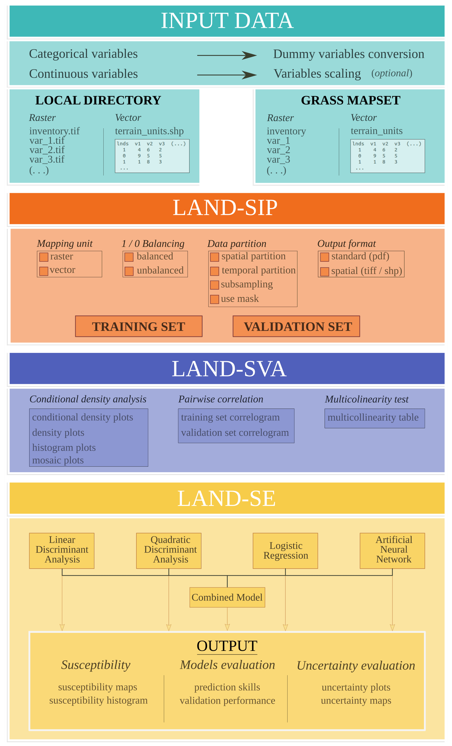
The common LAND-SUITE run starts with LAND-SIP, which is able to execute LAND-SVA and successively LAND-SE in cascade. Alternatively, only one of these last two modules can be executed after LAND-SIP, depending on the user needs and on the type of software applications. The three modules can also be executed separately, as long as the user is able to provide the appropriate data input.
2.1 LAND-SIP: LANDslide – Susceptibility Input Preparation
LAND-SIP is designed for input preparation and has high relevance for susceptibility analysis because its main purpose is the subdivision and preparation of the training and validation datasets that will be used by the other two modules.
The dataset partition is controlled and customized by the user, who can select the type of the mapping unit (i.e., raster or polygons), choose the appropriate combination of variables, define the extent (i.e., using a mask) of the training and the validation areas, and choose the output types. This large number of options allows the user to decide and perform largely diversified types of susceptibility applications. LAND-SIP allows the user to select different functionalities and criteria to partition the training and validation datasets.
-
Balanced or unbalanced random sampling. In the balanced sampling, an equal number of mapping units with grouping values equal to 0 and 1 are selected randomly. Conversely, in the unbalanced sampling the proportions of mapping units with grouping values equal to 0 and 1 is different and is defined by the user. In the raster-based analyses, the user may choose two ways to select the mapping units with landslides: (i) pixel sampling based on a pixel's random sampling within mapped landslides and (ii) landslide sampling based on a random landslide sampling (using an additional landslide vector layer), whereby all the pixels of a selected landslide are considered either part of the training or of the validation datasets.
-
Subsampling or sampling reducing partitions. In subsampling the size of the original dataset is randomly reduced by the user by specifying the proportion of data used. This criterion is particularly helpful for preliminary investigations, in applications with large datasets, or in the case of limited computation resources.
-
Spatially or temporally based datasets partition. This criterion uses different input layers for the training and validation.
-
Combinations of the criteria described above can also be used.
The criteria are fully customizable by the user. Once a given criterion is chosen and training and validation datasets correctly partitioned, all the subsequent analyses will be performed accordingly. As previously mentioned, such datasets are always stored in RDATA format to guarantee full data handling and control. Detailed information on LAND-SIP configurations can be found in the user guide.
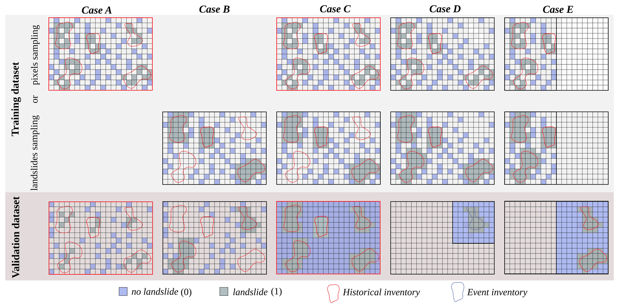
Figure 2Simplified representations of the five LAND-SUITE applications, referred to as “cases” in the figures and text, representing common susceptibility investigations. Red boxes highlight the cases described in the application (Sect. 4).
The flexibility of the choices in the configuration phase allows the user to draw and execute many diversified susceptibility applications. It is out of the scope of this paper, if not impossible, to identify all the possible potential software applications. However, in the following, five applications (hereafter referred to as “cases”) are listed and discussed with the purpose of explaining how LAND-SIP, and in turn LAND-SUITE, can be configured and used for executing the most common susceptibility investigations (Fig. 2).
-
In Case A the susceptibility modeling is performed by applying a regular cross-validation approach. A balanced random sampling is used to select the grouping variable mapping units following the “pixel sampling” selection criteria, with the size of training and validation datasets (e.g., 70 % training and 30 % validation) selected by the user (Fig. 2, Case A). This configuration is usually applied for exploratory analysis mainly focused on the preliminary evaluation of the explanatory variables (see LAND-SVA section) and of the statistical performance of the model. This execution can be performed by the user to select, add, or remove explanatory variables before the application of the trained model to the entire study area (Case C).
-
In Case B the application considers a cross-validation approach similar to Case A, but the training and validation dataset partition uses the “landslide sampling” selection criteria. As before, a balanced random sampling and a specific size of the training and validation datasets (e.g., 70 % training and 30 % validation) are chosen (Fig. 2, Case B). As in Case A, it can be used to analyze the explanatory variables and to test the modeling results as well as its dependency from the selection of different landslide samples.
-
In Case C the training configuration can be similar either to Case A or B, but the validation is applied to the entire study area. This case should be applied when the definitive set of explanatory variables is selected and the statistical performance of the model is satisfactory and acceptable. The validation map will show the susceptibility zonation for the entire extent of the study area (Fig. 2 Case C).
-
Case D performs a temporal validation, applicable when a geomorphological–historical inventory map is available to train the model and an event (or a successive) landslide inventory map is used for validation. In such a case the landslide event map used for the model validation may cover only a portion of the study area, with a spatial extent different from the inventory map used for the calibration (Fig. 2 Case D). This configuration requires two different mask files, one covering the entire study area and the other only the area affected by the event. The selection of the explanatory variables and the preliminary evaluation of the model can be performed by applying Case A or B. The temporal validation may cover the entire study area when an event inventory is available for its total extent.
-
Case E performs a spatial validation, with the model calibration performed in a given region of the study area and the validation in a different one. For example, the model training and validation can be performed in two contiguous but not overlapping river basins. In such a case, the variable selection and the preliminary model testing could be performed only in one of the two basins, similarly to Case A or B. In this case the explanatory variables and landslide inventory map should be available in the two regions with the same characteristics (Fig. 2 Case E). This configuration requires two different landslide inventory maps, two mask files and two explanatory variables datasets, respectively, for the calibration and for the validation region.
2.2 LAND-SVA: LANDslide – Susceptibility Variable Analysis
LAND-SVA is designed for the explorative analysis of the LAND-SE training and validation input datasets and facilitates the selection of the optimal set of variables. The tool automatically detects continuous or dummy variables (i.e., derived from categorical data and normally represented with numerical discrete values) and selects the outputs accordingly. All the analyses are performed separately for the training and validation datasets, with the main purpose of providing the possibility to analyze and control the dataset differences.
In this step, the user may decide whether or not to scale the variables, and the option is applied jointly to the two datasets to guarantee the comparability and applicability of the trained susceptibility model to the validation datasets. The variable scaling introduces advantages, particularly during numerical model convergence, avoiding working with variables with diversified ranges. However, two susceptibility analyses, performed with scaled or non-scaled variables, lead to the same results when both are able to converge. It is important to note that two analyses performed using scaled variables in two different areas do not necessarily guarantee the comparability of the variable coefficients. Similarly, such comparability does not hold for coefficients of variables derived at different data resolutions (e.g., coefficients of slope derived using two different DEM resolutions; DEM: digital elevation model).
LAND-SVA performs the following analyses on continuous and categorical input variables (Figs. 3 and 4, Table 1).
-
Conditional density analysis (Fig. 3) includes the following.
-
Density plots for continuous variables that show the distribution of the values of numeric variables, stratified by the corresponding grouping variable value (0 and 1). Such plots use a kernel density estimator to show the probability density function of the variable. It basically corresponds to a smoothed version of a histogram plot and can be interpreted similarly.
-
Conditional density plots for continuous variables that examine the proportion of the grouping variable values (0 and 1) against the variation of a given continuous variable.
-
Histogram plots for categorical variables that, similarly to density plots, show the distribution of the values of categorical variables stratified by the corresponding grouping variable value (0 and 1). These plots use a normalized histogram counting to estimate the probability density function.
-
Mosaic plots for categorical variables that, similarly to conditional density plots, show the proportion of the grouping variable values (0 and 1) for different variable categories.
-
-
Pairwise correlation analysis (Fig. 4) of the input variables: in the analysis a correlogram chart and a correlation matrix are prepared to show pairwise correlation statistics among the different explanatory variables. The correlogram shows the following: in the upper triangular matrix, the values of the Pearson correlation coefficient for each pair of variables (i.e., R coefficient ranging between −1 and 1, respectively, for a perfect negative and positive correlation); in the lower triangular matrix, a graphical representation of the level of correlation (i.e., flattened negatively and positively oriented ellipses, respectively, for a negative and positive correlation); in the diagonal, the R value for the correlation of a variable with itself (R = 1). Colors indicate different levels of correlation (i.e., white for no correlation, red and blue, respectively, for negative and positive correlations).
-
Multicollinearity test (Table 1) of the input variables: the analysis follows the diagnostic procedures described by Belsley et al. (1980), which examines the conditioning of the matrix of independent variables by computing a test statistic called the condition index. In LAND-SVA, a multicollinearity table is prepared to identify multicollinearity among the explanatory variables. Multicollinearity exists whenever a variable is highly correlated with one or more of the other variables and represents a problem undermining the statistical significance of the independent variables. Multicollinearity implies that one variable in a multiple regression model can be linearly predicted from the others with a substantial degree of accuracy.

Figure 3Example of the conditional density analysis outputs generated by LAND-SVA for five synthetic explanatory variables.
Some guidance is provided for the interpretation of the conditional density outputs shown in Fig. 3. The density and histogram plots highlight significant numerical and categorical variables when the distributions of the values corresponding to the grouping variable categories (0 or 1) are significantly different (i.e., different shapes and lack of overlapping). Only under these circumstances, a variable may have high significance in the modeling. The conditional density and mosaic plots need to be interpreted considering the variation and trend of the proportion of the grouping variable categories (i.e., the proportion of 0 or 1 along the vertical axis) along with the variable value (i.e., along the horizontal axis). A distinct increase or decrease in such proportion, along with a reduced oscillation of it, and without lack of data, is the expected behavior to identify a variable significantly contributing to the susceptibility zonation. Under these circumstances, an independent explanatory variable may have an unambiguous effect on the dependent grouping variable used in the modeling (i.e., the presence or absence of landslides in the mapping unit). Following these considerations, only the variables A and D should be considered in the susceptibility modeling (Fig. 3).
The pairwise correlation analysis and multicollinearity test are easier to interpret. When a significant high correlation is detected among two or more variables, one or more of the correlated variables should be excluded from the analysis. This is relevant for the following reasons.
-
The joint use of two or more correlated variables does not introduce a significant advance for the multivariate modeling.
-
Generally, multivariate models assume independence among explanatory variables and when correlation exists, the independence assumption is not verified.
-
When the degree of correlation among variables is high, it can introduce problems during the model fitting and for the interpretation of the model results.
-
Multicollinearity can introduce two main types of problems: (i) the coefficient estimates can vary largely depending on the other independent variables considered in the model, with such coefficients' values becoming very sensitive to small model changes. (ii) Multicollinearity may reduce the precision of the estimated coefficients, weakening the statistical significance of the model and leading to a limited p-value reliability when identifying statistically significant independent variables.
-
When collinearity occurs, the model coefficient values and their signs may change significantly depending on the specific variables included in the model, leading to difficulties evaluating the results. Slightly different models may lead to different conclusions, making the actual contribution of variables impossible to understand.
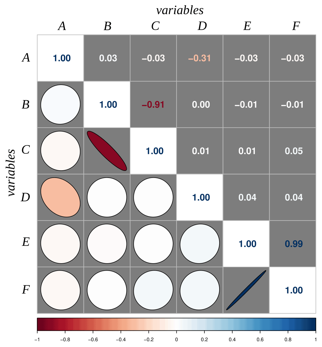
Figure 4Example of the graph showing the output of the pairwise correlation analysis generated by LAND-SVA.
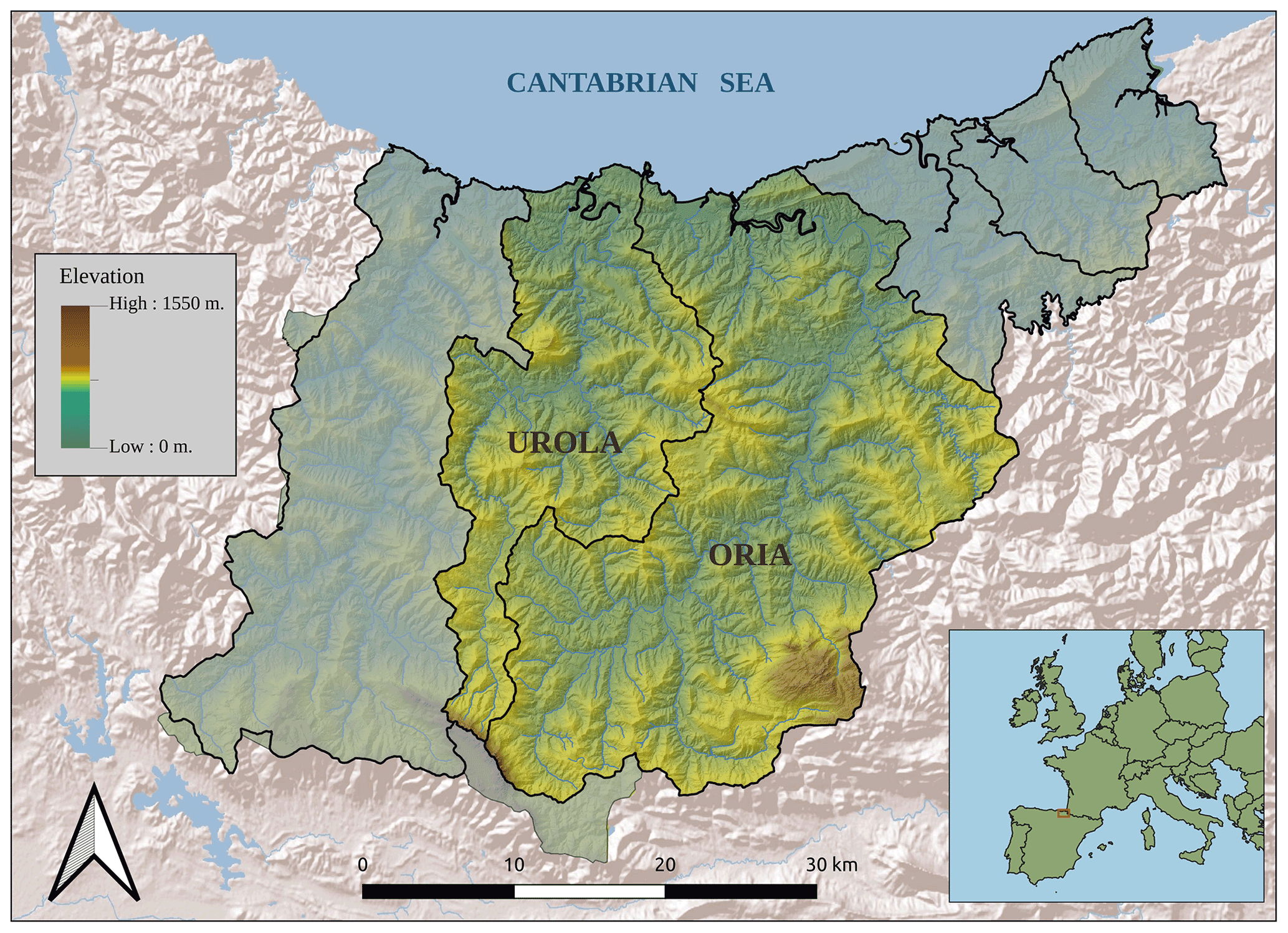
Figure 5Location of the Gipuzkoa Province study area and the two river basins Urola and Oria.
Pairwise correlated variables are those with Pearson R values in the correlogram matrix close to +1 or −1 (Fig. 4). Instead, multicollinearity is detected when the test statistic (i.e., the condition index in Table 1) is greater than 30 (Belsley, 1991). When a large condition index (rows with condition index >30) is associated with two or more variables with large variance decomposition proportions (values corresponding to variables >0.5), these variables may cause collinearity problems. Based on the above considerations, the variables B, C, E, and F show multicollinearity (Table 1) and the correlogram (Fig. 4) helps to identify correlations between B and C and between E and F. These results suggest alternatively excluding B or C (negatively correlated) and E or F (positively correlated).
Table 1Example of the table showing the output of the multicollinearity test generated by LAND-SVA.

2.3 LAND-SE: LANDslide – Susceptibility Evaluation
LAND-SE is the module for landslide susceptibility modeling and zonation that is described in detail in Rossi and Reichenbach (2016). The software holds the possibility to perform and combine different statistical susceptibility modeling methods, evaluate the results, and estimate the associated uncertainty. In particular, it allows for (i) the selection of different combinations of multivariate approaches; (ii) the evaluation of the model prediction skills and performances using success contingency matrices and plots, ROC (receiver operating characteristic) curves, and prediction rate curves; (iii) the estimation of the associated uncertainty and errors; (iv) the production of results in standard geographical formats (shapefiles, geotiff); and (v) the usage of additional computational parameters to tune the calculation procedure for the analysis of large datasets.
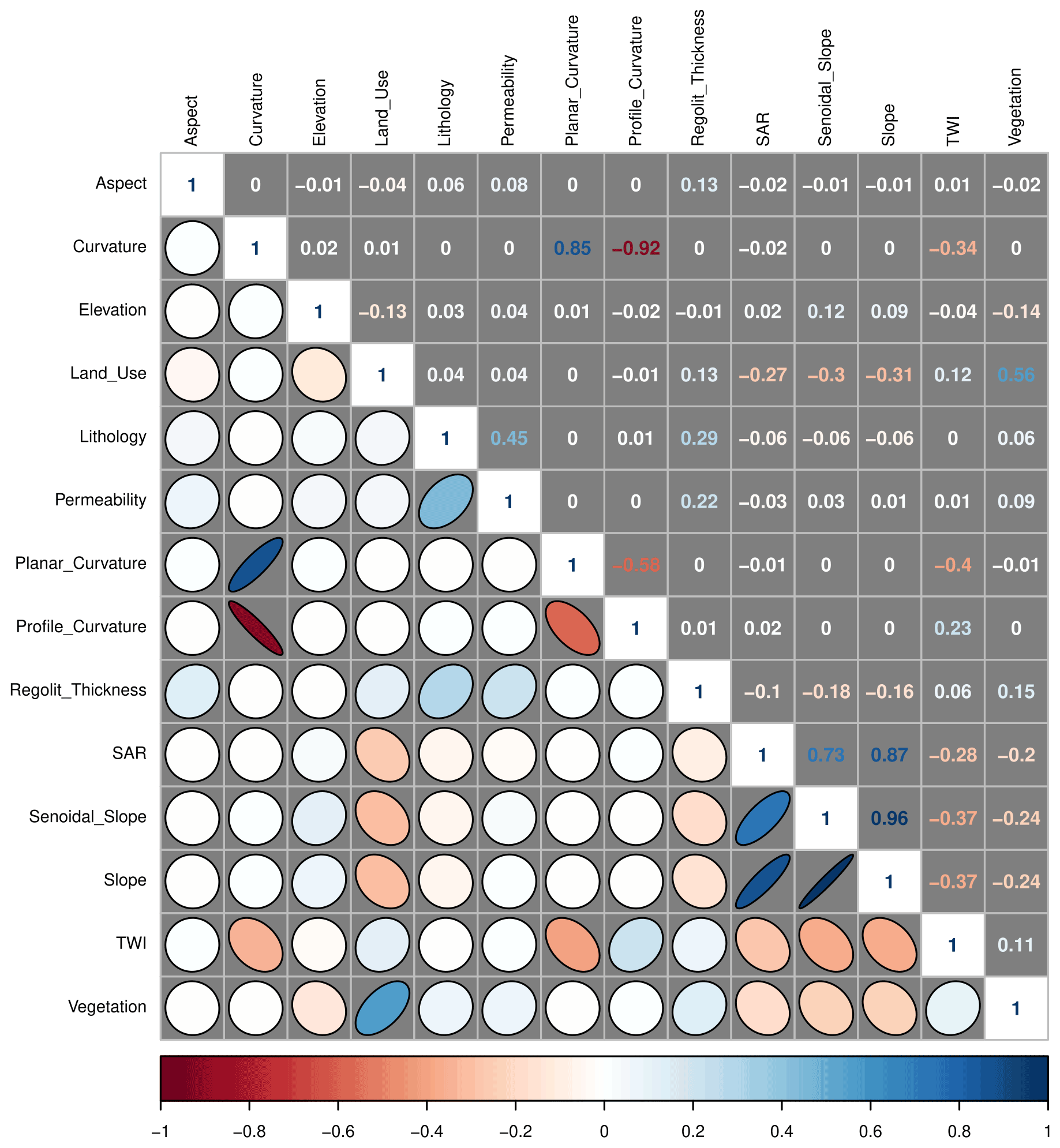
Figure 6The figure shows the correlogram obtained by LAND-SVA for the complete set of variables available in the Gipuzkoa study area (Case A).
The basic LAND-SE execution flow involves the following steps:
-
the single susceptibility models' executions and zonation production;
-
the combination of the single susceptibility models using a logistic regression approach;
-
the evaluation of the single and combined susceptibility models; and
-
the estimation of the uncertainty of the single and combined susceptibility models.
Additional details on the LAND-SE tool specifications, configuration, functioning, and scientific assumption can be found in Rossi and Reichenbach (2016), Rossi et al. (2010), and the LAND-SUITE user guide.
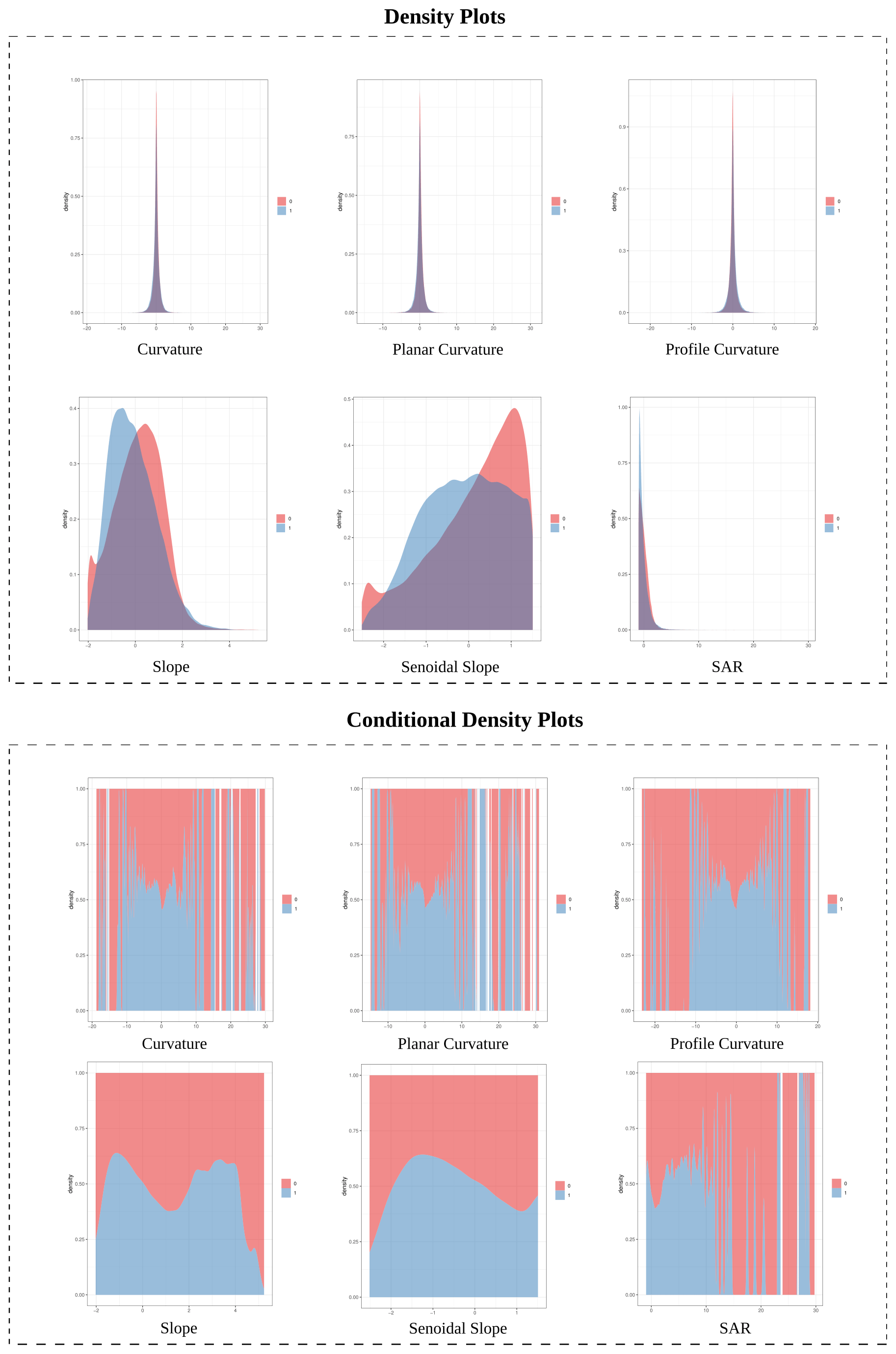
Figure 7Density plots and conditional density plots for some continuous explanatory variables available in the Gipuzkoa study area.
To better illustrate the LAND-SUITE functionalities, we selected a portion of the study area located in the Gipuzkoa Province (northern sector of the Iberian Peninsula), where a landslide inventory and 14 explanatory variables were mapped (Bornaetxea et al., 2018). This set of thematic data is used to describe different applications of LAND-SUITE (i.e., Case A and C in Fig. 2) and to provide examples of the susceptibility analysis outputs, including plots and maps. The critical discussion of results and their scientific relevance is out of the scope of this article and requires dedicated analysis, such as those described by Bornaetxea et al. (2018) and Rossi et al. (2021).
3.1 Description of the study area and available data
The Gipuzkoa Province is located in the northern part of the Iberian Peninsula along the western end of the Pyrenees and covers an area of 1980 km2, with an altitude ranging from sea level to 1528 m a.s.l. The province, characterized by a steep morphology, is subdivided into six main watersheds that drain the territory toward the Cantabrian Sea (Fig. 5). The investigated area is lithologically heterogeneous, with materials ranging from Paleozoic rocks to Quaternary deposits, corresponding to a hilly and mountainous Atlantic landscape (Mücher et al., 2010). The average annual precipitation is 1597 mm (González-Hidalgo et al., 2011) with two maximum rainy seasons: November–January and April.
The landslide inventory was prepared by an experienced geomorphologist during field surveys. The map shows the location and shape of 793 individual landslides in polygon format, mainly classified as shallow mass movements. A total of 14 geo-environmental maps were available as explanatory variables. Morphometric variables, such as elevation, slope, sinusoidal slope (Santacana Quintas, 2001; Amorim, 2012), aspect, surface area ratio (SAR), terrain wetness index (TWI), curvature, plan curvature, and profile curvature, were derived from a DEM with a 5 m × 5 m spatial resolution. Lithology, permeability, regolith thickness, land use, and vegetation were downloaded from the official spatial data repository of the Basque Country (GeoEuskadi). Relative landslide incidence, by means of the frequency ratio (Bonham-Carter, 1994; Lee et at., 2002), was used to assign a numerical value to each category (hence transformed into dummy variables). For simplicity, we limited the model application to the two central and largest watersheds, which correspond to the Urola and Oria basins.
3.2 LAND-SIP: preparation of the training and validation datasets
Among all the possible LAND-SUITE applications, we selected the cross-validation approach with the pixel sampling method (Case A). Moreover, we applied the balanced random sampling criteria to select the same number of pixels with and without landslides for both the training and validation datasets. The susceptibility model was calibrated using 70 % of the data and validated using the remaining 30 %.
As a first step, using LAND-SVA, we performed a preliminary evaluation of the available data. After the selection of the most significant explanatory variables, we evaluated the statistical performance of the calibrated model with the inspection of the susceptibility outputs produced by LAND-SE. At the final step, we applied Case C (Fig. 2) to obtain a susceptibility zonation for the entire area.
3.3 LAND-SVA: variable analysis and selection for the training and validation datasets
We selected Case A and ran LAND-SVA with the complete set of variables for the explorative analysis of training and validation datasets in order to select the optimal combination of explanatory variables. The multicollinearity table (Table 2) shows one condition index larger than 30 and one close to this value (29 722), with variance decomposition proportion values larger than 0.5. Thereby, the test detected two groups of variables (group I: curvature, planar curvature, and profile curvature; group II: SAR, slope, senoidal slope) with multicollinearity problems.
Table 2Multicollinearity table generated by LAND-SVA for the Gipuzkoa study area.
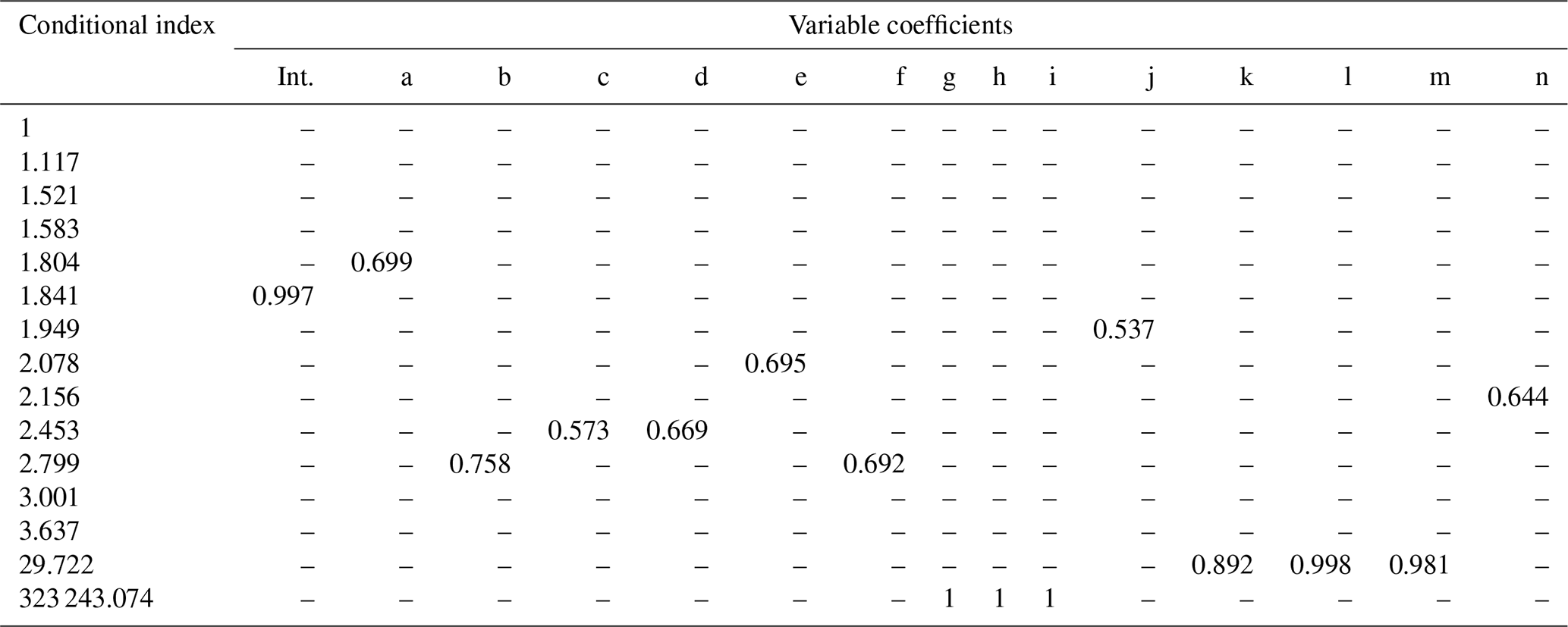
Int: intercept, a: aspect, b: land use, c: lithology, d: permeability, e: regolith thickness, f: vegetation, g: curvature, h: planar curvature, i: profile curvature, j: elevation, k: SAR, l: slope, m: senoidal slope, n: TWI.
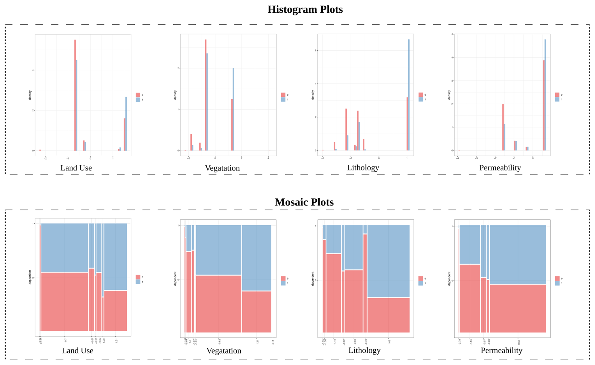
Figure 8Histogram plots and mosaic plots for two categorical explanatory variables available in the Gipuzkoa study area.
Inspection of the correlogram (Fig. 6) confirms the pairwise correlations within groups I and II and highlights an additional correlation between vegetation and land use, assuming a Pearson R absolute value of 0.5 as a threshold for detecting correlations.
To obtain additional information on the highly correlated continuous variables, the relation of each explanatory layer with the dependent variable was analyzed through the density plots and conditional density plots reported in Fig. 7. Similarly, we checked the histogram plots and mosaic plots (Fig. 8) to analyze the categorical variables. All the remaining outputs of the conditional density analysis were also evaluated, to check their relevance for the susceptibility modeling.
The evaluation of LAND-SVA outputs allowed the following:
-
the removal of all the variables in group I due to high correlation and to the lack of relevant differences between 1 and 0 in the density plots and conditional plots;
-
the selection of slope in group II based on the better distribution separation and trend shown in the density and conditional plots; and
-
the selection of both vegetation and land use, with a weak correlation, confirmed by their Pearson R values only slightly higher than 0.5.
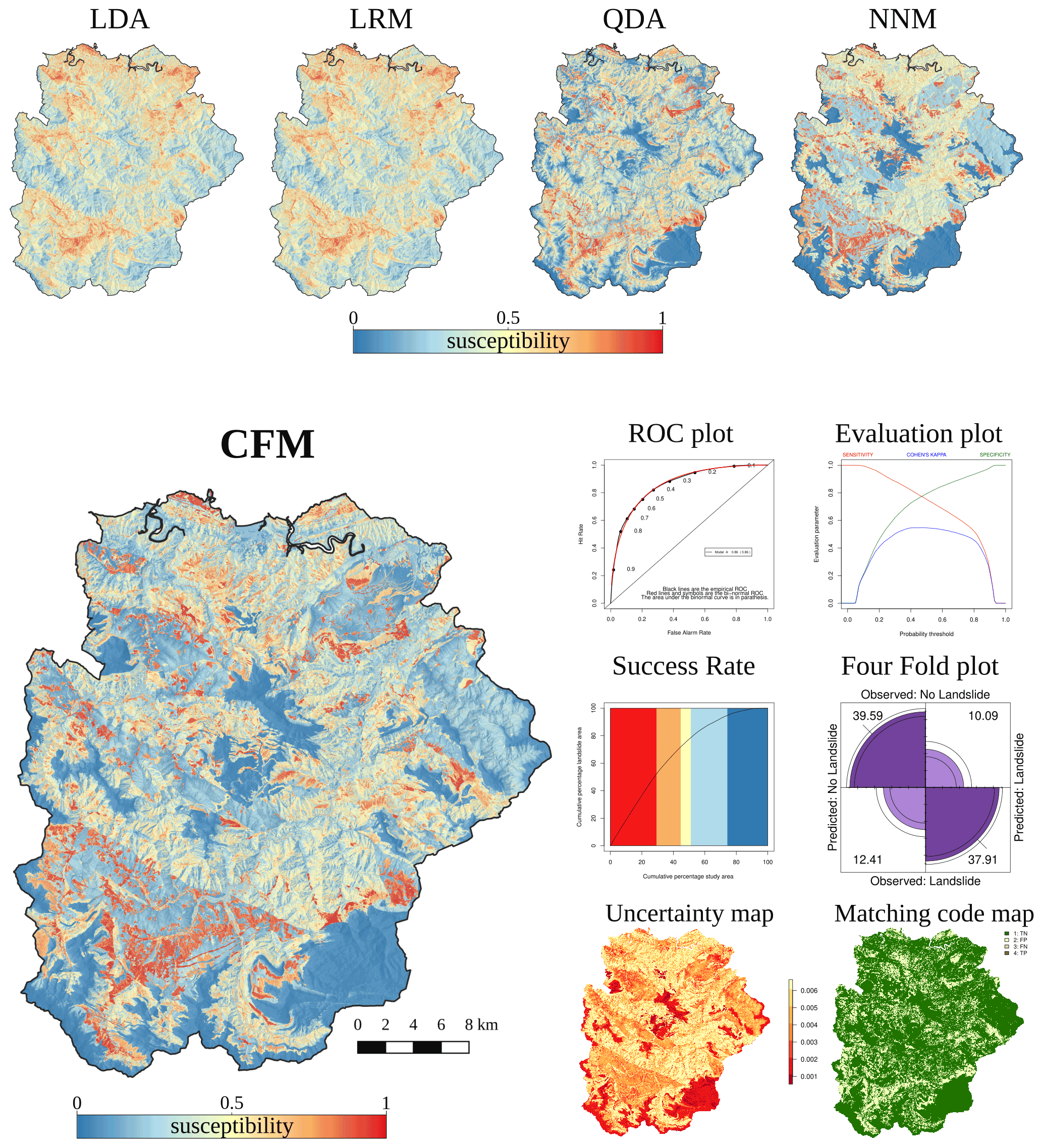
Figure 9Examples of the most relevant outputs of LAND-SE obtained in the Gipuzkoa study area. LDA: linear discriminant analysis; LRM: logistic regression model; QDA: quadratic discriminant analysis; NNM: neural network analysis; CFM: combined model function.
3.4 LAND-SE: susceptibility of model execution and zonation production
After the analysis of the results produced by LAND-SVA, the final set of explanatory variables used to run LAND-SE included aspect, land use, lithology, permeability, regolith thickness, vegetation, elevation, slope, and topographic wetness index. The same training set was used to prepare the four single landslide susceptibility models and the combined model (Fig. 9). The figure shows the different landslide zonation maps and the plots (i.e., ROC plot, evaluation plot, success rate plot, and contingency or fourfold plot) used to evaluate the training performance of the combined model. The two small maps at the bottom illustrate the errors and uncertainty values associated with the combined susceptibility model (Rossi et al, 2010). This set of outputs, restituted by LAND-SE, is commonly used for the verification and analysis of the susceptibility zonations obtained by LAND-SUITE.
LAND-SUITE was developed to support the landslide susceptibility inference process, which is a complex task. LAND-SUITE includes a suite of tools for statistically based landslide susceptibility zonation implemented in R and released with an open-source license. As highlighted by Reichenbach et al. (2018), there are only a reduced number of scientific contributions on statistical landslide susceptibility modeling, properly selecting and combining the suitable variables, and applying the relevant statistical evaluations for realizing high-quality zonations. This is mainly due to the lack of a comprehensive and shared approach for susceptibility modeling. LAND-SUITE can be used for the preparation and selection of the variables and/or data required for a reliable statistical analysis, and it is designed to support the geomorphological–geological experience and competence of the operator. LAND-SUITE facilitates and simplifies the testing of diversified geomorphological hypotheses, allowing the verification and discussion of the initial modeling assumptions, the preparation of less subjective statistically based susceptibility zonation, and the evaluation of the quality of the modeling results. A key step for a reliable landslide susceptibility modeling is the preparation of robust and unbiased input data, which largely depends on the user's skill and experience. In many cases, the data classification approaches as well as the reliability and representativeness of the thematic information are more important than the statistical methods and tools used for the landslide susceptibility estimation. Low-quality output and errors often derive from incomplete or non-significant data. The tool has the ambition to help a skilled user with the preparation of statistically correct and robust models, allowing easily applying and testing different classical statistical procedures (e.g., random sampling, data scaling, use of common machine learning approaches, and commonly used evaluation metrics).
Using LAND-SUITE, the user can compare results of different mapping units (e.g., pixel, slope units, administrative units) with distinct configurations and data resolution at diverse spatial scales. LAND-SUITE does not consider all the statistical approaches for landslide susceptibility modeling and zonation, which can be potentially included in future software upgrades. Possible LAND-SUITE advancements can also be achieved by implementing new procedures to evaluate the variables' significance across the different statistical approaches.
The suite has high flexibility and allows performing different partitions of the training and validation dataset as well as diversified validation tests (e.g., temporal, spatial, cross-validation), which are relevant evaluation steps to realize robust scientific susceptibility modeling exercises.
LAND-SUITE can be used to model and evaluate the spatial probability of the occurrence of other types of natural phenomena (such as floods, forest fires, and rockfall source areas; see, e.g., Rossi et al., 2021), and this use may highlight the need for specific code modifications and refinements.
LAND-SUITE is composed of three modules (LAND-SIP, LAND-SVA, LAND-SE) coded as separate R script files and can be executed under different operating systems. The software was mainly tested under WindowsOS and LinuxOS, with the version of R-4.1.1 (64-bit). Some code functionalities of LAND-SIP require GRASS GIS binding. We tested the script using GRASS GIS version 7 under WindowsOS and LinuxOS. We recommend LinuxOS due to the better software integration at a bash scripting level. LAND-SUITE is free software; it can be redistributed or modified under the terms of the GNU General Public (either version 2 of the license or any later version) as published by the Free Software Foundation. The program is distributed in the hope that it will be useful, but without any warranty, without even the implied warranty of merchantability or fitness for a particular purpose. See the GNU General Public License for more details. LAND-SUITE V1.0 is archived in the Zenodo repository at https://doi.org/10.5281/zenodo.5650810 (Rossi and Bornaetxea, 2021).
In this work, example data have been used only to show different LAND-SUITE applications and they are not needed to apply LAND-SUITE elsewhere. The software can in fact be used in other areas using the appropriate input data. Upon request, the authors can provide the Gipuzkoa data used in the analyses to allow replication of the results.
The supplement related to this article is available online at: https://doi.org/10.5194/gmd-15-5651-2022-supplement.
MR conceptualized the work, designed the overall methodology behind the software, and supervised the research activity. MR wrote the core of codes LAND-SIP, LAND-SVA, and LAND-SE. TB implemented specific functionalities of LAND-SIP and LAND-SVA, reviewed the codes, and performed the overall LAND-SUITE code validation and testing. PR participated in the LAND-SUITE code validation and testing. MR wrote the original draft of the paper. TB and PR largely contributed to the review, editing, and writing of the paper.
The contact author has declared that none of the authors has any competing interests.
Publisher's note: Copernicus Publications remains neutral with regard to jurisdictional claims in published maps and institutional affiliations.
We thank the editor and the anonymous reviewers for their valuable comments and suggestions.
The implementation and improvement of LAND-SUITE with respect to the version published by Rossi and Reichenbach (2016) were funded mainly using internal funds. Txomin Bornaetxea was financially supported by the postdoctoral fellowship program of the Basque Government (grant numbers POS_2020_2_0010) and hosted by the University of the Basque Country (UPV/EHU, group IT1678) in the framework of a scientific collaboration with the Geological Survey of Canada as well as during scientific collaborations with the Geomorphological Group of the Research Institute for the Geo-Hydrological Protection in Perugia, Italian National Research Council (CNR-IRPI).
This paper was edited by Le Yu and reviewed by two anonymous referees.
Aleotti, P. and Chowdhury, R.: Landslide hazard assessment: summary review and new perspectives, B. Eng. Geol. Environ., 58, 21–44, 1999.
Amorim, S. F.: Estudio comparativo de métodos para la evaluación de la susceptibilidad del terreno a la formación de deslizamientos superficiales: Aplicación al Pirineo Oriental, PhD, Universidad Politécnica de Catalunya, Barcelona, http://futur.upc.edu/10953986 (last access: 6 July 2022), 2012.
Baum, R. L., Savage, W. Z., and Godt, J. W.: TRIGRS: a Fortran program for transient rainfall infiltration and grid-based regional slope-stability analysis, version 2.0, Reston, VA, USA: US Geological Survey, 2008–1159, 2008.
Belsley, D. A.: A guide to using the collinearity diagnostics, Comput. Sci. Eco. Manage., 4, 33–50, 1991.
Belsley, D. A., Kuh, E., and Welsch, R. E. (Eds.): Regression Diagnostics, John Wiley and Sons, New York, https://doi.org/10.1002/0471725153, 1980.
Bonham-Carter, G. F.: Geographic information systems for geoscientists-modeling with GIS, Comput. Meth. Geosci., 13, 398 pp., 1994.
Bornaetxea, T., Rossi, M., Marchesini, I., and Alvioli, M.: Effective surveyed area and its role in statistical landslide susceptibility assessments, Nat. Hazards Earth Syst. Sci., 18, 2455–2469, https://doi.org/10.5194/nhess-18-2455-2018, 2018.
Bragagnolo, L., da Silva, R. V., and Grzybowski, J. M. V.: Landslide susceptibility mapping with r, landslide: A free open-source GIS-integrated tool based on Artificial Neural Networks, Environ. Modell. Softw., 123, 104565, https://doi.org/10.1016/j.envsoft.2019.104565, 2020.
Brenning, A.: Statistical geocomputing combining R and SAGA: The example of landslide susceptibility analysis with generalized additive models, in: SAGA–Seconds Out, Hamburger Beiträge Zur Physischen Geographie und Landschaftsökologie, Vol. 19, edited by: Böhner, J., Blaschke, T., Montanarella, L., 23–32, 2008.
Chacón, J., Irigaray, C., Fernandez, T., and El Hamdouni, R.: Engineering geology maps: landslides and geographical information systems, Bull. Eng. Geol. Environ., 65, 341–411, https://doi.org/10.1007/s10064-006-0064-z, 2006.
Fell, R., Corominas, J., Bonnard, C., Cascini, L., Leroi, E., and Savage, W. Z.: Guidelines for landslide susceptibility, hazard and risk zoning for land-use planning, Eng. Geol., 102, 99–111, 2008.
Dietrich, W. E. and Montgomery, D. R.: SHALSTAB: a digital terrain model for mapping shallow landslide potential, University of California, http://calm.geo.berkeley.edu/geomorph/shalstab/index.htm (last access: 7 July 2022), 1998.
González-Hidalgo, J. C., Brunetti, M., and de Luis, M.: A new tool for monthly precipitation analysis in Spain: MO-PREDAS database (monthly precipitation trends December 1945–November 2005), Int. J. Climatol., 31, 715–731, https://doi.org/10.1002/joc.2115, 2011.
Guzzetti, F., Reichenbach, P., Cardinali, M., Galli, M., and Ardizzone, F.: Probabilistic landslide hazard assessment at the basin scale, Geomorphology, 72, 272–299, https://doi.org/10.1016/j.geomorph.2005.06.002, 2005.
Guzzetti, F., Reichenbach, P., Ardizzone, F., Cardinali, M., and Galli, M.: Estimating the quality of landslide susceptibility models, Geomorphology, 81, 166–184, https://doi.org/10.1016/j.geomorph.2006.04.007, 2006.
Huabin, W., Gangjun, L., Weiya, X., and Gonghui, W.: GIS-based landslide hazard assessment: an overview. Prog. Phys. Geogr., 29, 548–567, 2005.
Kanungo, D. P., Arora, M. K., Sarkar, S. and Gupta, R. P.: Landslide Susceptibility Zonation (LSZ) mapping – A Review, J. South Asia Disaster Studies, 2, 81–105, 2009.
Lee, S. and Min, K.: Statistical analysis of landslide susceptibility at Yongin, Korea, Environ. Geol., 40, 1095–1113, https://doi.org/10.1007/s002540100310, 2001.
Lee, S., Chwae, U., and Min, K.: Landslide susceptibility mapping by correlation between topography and geological structure: the Janghung area, Korea, Geomorphology, 46, 149–162, https://doi.org/10.1016/S0169-555X(02)00057-0 2002.
Mergili, M., Marchesini, I., Alvioli, M., Metz, M., Schneider-Muntau, B., Rossi, M., and Guzzetti, F.: A strategy for GIS-based 3-D slope stability modelling over large areas, Geosci. Model Dev., 7, 2969–2982, https://doi.org/10.5194/gmd-7-2969-2014, 2014.
Mücher, C. A., Klijn, J. A., Wascher, D. M., and Scham-inée, J. H.: A new European Landscape Classification (LAN-MAP): A transparent, flexible and user-oriented method-ology to distinguish landscapes, Ecol. Indic., 10, 87–103, https://doi.org/10.1016/j.ecolind.2009.03.018, 2010.
Osna, T., Sezer, E. A., and Akgun, A.: GeoFIS: an integrated tool for the assessment of landslide susceptibility, Comput. Geosci., 66, 20–30, https://doi.org/10.1016/j.cageo.2013.12.016, 2014.
Pack, R. T., Tarboton, D. G., and Goodwin, C. N.: The SINMAP approach to terrain stability mapping, https://digitalcommons.usu.edu/cee_facpub/2583/ (last access: 6 July 2022), 1998.
Pardeshi, S. D., Autade, S. E., and Pardeshi, S. S.: Landslide hazard assessment: recent trends and techniques, Springer Plus, 2, 1–11, 2013.
R Core Team: R: A language and environment for statistical computing, R Foundation for Statistical Computing, Vienna, Austria, https://www.R-project.org/, last access: 20 September 2021.
Reichenbach, P., Rossi, M., Malamud, B. D., Mihir, M., and Guzzetti, F.: A review of statistically based landslide susceptibility models, Earth-Sci. Rev., 180, 60–91, https://doi.org/10.1016/j.earscirev.2018.03.001, 2018.
Rossi, G., Catani, F., Leoni, L., Segoni, S., and Tofani, V.: HIRESSS: a physically based slope stability simulator for HPC applications, Nat. Hazards Earth Syst. Sci., 13, 151–166, https://doi.org/10.5194/nhess-13-151-2013, 2013.
Rossi, M. and Bornaetxea, T.: LAND-SUITE V1.0: a suite of tools for statistically-based landslide susceptibility zonation, Zenodo [code], https://doi.org/10.5281/ZENODO.5650810, 2021.
Rossi, M. and Reichenbach, P.: LAND-SE: a software for statistically based landslide susceptibility zonation, version 1.0, Geosci. Model Dev., 9, 3533–3543, https://doi.org/10.5194/gmd-9-3533-2016, 2016.
Rossi, M., Guzzetti F., Reichenbach P., Mondini A. C., and Peruccacci S.: Optimal landslide susceptibility zonation based on multiple forecasts, Geomorphology, 114, 129–142, https://doi.org/10.1016/j.geomorph.2009.06.020, 2010.
Rossi, M., Sarro, R., Reichenbach, P., and Mateos, R. M.: Probabilistic identification of rockfall source areas at regional scale in El Hierro (Canary Islands, Spain), Geomorphology, 381, 107661, https://doi.org/10.1016/j.geomorph.2021.107661, 2021.
Santacana Quintas, N.: Análisis de la susceptibilidad del terreno a la formación de deslizamientos superficiales y grandes deslizamientos mediante el uso de sistemas de información geográfica, Aplicación a la cuenca alta del río Llobregat, PhD, Universitat Politècnica de Catalunya, Barcelona, https://www.tdx.cat/handle/10803/6213, 2001.
Sahin, E. K., Colkesen, I., Acmali, S. S., Akgun, A., and Aydinoglu, A. C.: Developing comprehensive geocomputation tools for landslide susceptibility mapping: LSM tool pack, Comput. Geosci., 144, 104592, https://doi.org/10.1016/j.cageo.2020.104592, 2020.
Simoni, S., Zanotti, F., Bertoldi, G., and Rigon, R.: Modelling the probability of occurrence of shallow landslides and channelized debris flows using GEOtop-FS, Hydrol. Process., 22, 532–545, 2008.
van Westen, C. J.: Statistical landslide hazard analysis, ILWIS 2.1 for Windows application guide, ITC publication, 2, 73–84, 1997.
van Westen, C. J., Castellanos, E., and Kuriakose, S. L.: Spatial data for landslide susceptibility, hazard, and vulnerability assessment: An overview, Eng. Geol.,, 102, 112–131, 2008.