the Creative Commons Attribution 4.0 License.
the Creative Commons Attribution 4.0 License.
 | 14 Jul 2022
Effects of point source emission heights in WRF–STILT: a step towards exploiting nocturnal observations in models
Fabian Maier
Christoph Gerbig
Ingeborg Levin
Ingrid Super
Julia Marshall
Samuel Hammer
An appropriate representation of point source emissions in atmospheric transport models is very challenging. In the Stochastic Time-Inverted Lagrangian Transport model (STILT), all point source emissions are typically released from the surface, meaning that the actual emission stack height plus subsequent plume rise is not considered. This can lead to erroneous predictions of trace gas concentrations, especially during nighttime when vertical atmospheric mixing is minimal. In this study we use two Weather Research and Forecasting (WRF)–STILT model approaches to simulate fossil fuel CO2 (ffCO2) concentrations: (1) the standard “surface source influence (SSI)” approach and (2) an alternative “volume source influence (VSI)” approach where nearby point sources release CO2 according to their effective emission height profiles. The comparison with 14C-based measured ffCO2 data from 2-week integrated afternoon and nighttime samples collected at Heidelberg, 30 m above ground level shows that the root-mean-square deviation (RMSD) between modelled and measured ffCO2 is indeed almost twice as high during the night (RMSD =6.3 ppm) compared to the afternoon (RMSD =3.7 ppm) when using the standard SSI approach. In contrast, the VSI approach leads to a much better performance at nighttime (RMSD =3.4 ppm), which is similar to its performance during afternoon (RMSD =3.7 ppm). Representing nearby point source emissions with the VSI approach could thus be a first step towards exploiting nocturnal observations in STILT. The ability to use nighttime observations in atmospheric inversions would dramatically increase the observational data and allow for the investigation of different source mixtures or diurnal cycles. To further investigate the differences between these two approaches, we conducted a model experiment in which we simulated the ffCO2 contributions from 12 artificial power plants with typical annual emissions of 1 million tonnes of CO2 and with distances between 5 and 200 km from the Heidelberg observation site. We find that such a power plant must be more than 50 km away from the observation site in order for the mean modelled ffCO2 concentration difference between the SSI and VSI approach to fall below 0.1 ppm during situations with low mixing heights smaller than 500 m.
- Article
(2079 KB) - Full-text XML
- BibTeX
- EndNote


The Integrated Carbon Observation System (ICOS) research infrastructure was established to set up a dense European monitoring network of high-precision greenhouse gas measurements of concentrations and fluxes, therewith providing the observational basis to better understand the European carbon budget (Heiskanen et al., 2022). In Europe, one major challenge is the quantification of anthropogenic fossil fuel CO2 (ffCO2) emissions, but it is similarly important to understand “their redistribution among the atmosphere, ocean and terrestrial biosphere in a changing climate” (Friedlingstein et al., 2020). If the share of ffCO2 in the total continental signal is modelled correctly, the remaining biogenic share can be used as a top-down constraint on the continental biospheric CO2 fluxes (Basu et al., 2016). In this study, we use the term ffCO2 to refer to not only CO2 emissions resulting from the combustion of fossil fuels but also fossil CO2 emissions that occur during cement production. A well-established approach to determine the regional ffCO2 component in the observed atmospheric CO2 concentration is via Δ14CO2 measurements (e.g. Levin et al., 2003). Since CO2 emissions from fossil fuel combustion are devoid of 14C (the half-life of 14C is 5700 years; Currie, 2004), the atmospheric Δ14CO2 depletion measured in polluted areas relative to clean background air allows the regional (or “recently added”) ffCO2 surplus to be determined. Many studies have used this approach at various urban and rural sites (e.g. Levin et al., 2008; Turnbull et al., 2015; Wenger et al., 2019). Some 2-week integrated air samples and hourly flask samples are collected at ICOS class-1 stations for 14C analysis to estimate regional ffCO2 concentrations (Levin et al., 2020), thus helping to separate biospheric from fossil CO2 fluxes, e.g. in an inverse modelling framework (Wang et al., 2018; Basu et al., 2020).
Estimating ffCO2 fluxes from atmospheric CO2 and 14C measurements within an inverse modelling framework requires a correct representation of the atmospheric transport and mixing processes. Geels et al. (2007) evaluated five different Eulerian atmospheric transport models with continuous CO2 observations from various European sites, as well as aircraft flask samples, and showed that the model predictions are much better in the afternoon hours during well-mixed atmospheric conditions than during stable nocturnal conditions. That is why they recommend to only use afternoon observations from low-altitude sites to constrain CO2 sources or sinks. In addition, Lagrangian transport models like the Stochastic Time-Inverted Lagrangian Transport model (STILT) are very sensitive to the representation of the planetary boundary layer height (PBLH). STILT determines the sensitivity of atmospheric trace gas mixing ratios at an observation site to upwind surface fluxes (Lin et al., 2003). This so-called footprint defines the catchment area of the observation site, and in STILT it is by default sensitive to emissions from the bottom half of the planetary boundary layer (PBL). In STILT it is assumed that surface emissions are instantaneously mixed by turbulence in the bottom half of the PBL within one model time step. Gerbig et al. (2008) compared radiosonde-derived mixing heights with mixing heights derived from the European Centre for Medium-Range Weather Forecasts (ECMWF) meteorological data for 2 European summer months in 2005 and used STILT to assess the propagated uncertainty in the CO2 mole fraction. During daytime, they found no significant relative bias between radiosonde and ECMWF-derived mixing heights, but they found a relative standard deviation of about 40 % for the difference between both estimates. However, nighttime situations showed a relative bias of more than 50 % with a relative standard deviation of almost 100 %, meaning that the ECMWF-derived nocturnal mixing heights are on average larger compared to the radiosonde estimates. The authors showed that the 40 % uncertainty in daytime mixing heights already resulted in CO2 mole fraction uncertainties of 3 ppm on average during the 2 summer months studied, which corresponds to about 30 % of the simulated biogenic signals.
There is an additional problem in a time-reversed Lagrangian particle dispersion model (LPDM) like STILT, namely the incorrect representation of point source emissions. First, the calculated footprints are usually stored on a horizontal grid with limited resolution, which may lead to false attribution of point source emissions in cases where a higher-resolution footprint may actually have missed the point source. Since STILT dynamically coarsens the footprint resolution with distance to the receptor location, this problem may be more important for distant point sources. However, false attribution may also happen for nearby point sources due to a limited and inappropriate near-field footprint resolution. Second, point source emissions are often released from chimneys, whose stack height can be above the bottom half of the PBL during the night depending on the meteorological situation. However, in STILT the default is that all emissions, including point sources, are released from the ground and mixed into the bottom half of the PBL. Under stable conditions this can result in large overestimations of concentrations near the surface and large underestimations of concentrations above the PBL.

Figure 1(a) European ffCO2 point source emissions according to Super et al. (2020, red dots) and the locations of ICOS atmosphere class-1 and class-2 stations (black crosses). (b) ICOS atmosphere stations with a total of more than 1 million tonnes of ffCO2 emissions from point sources within a 50 km×50 km box around the station.
In central Europe, about 45 % of the ffCO2 emissions are released from point sources (Super et al., 2020), underlining the potential impact of these elevated emissions on downwind measurement sites. Figure 1 shows the distributions of ffCO2 point sources in Europe and illustrates how close some of the ICOS stations are located to these big ffCO2 point source emitters. An attempt was made to avoid station locations with strong emissions in the vicinity when designing the ICOS atmosphere station network. Nevertheless, there are eight ICOS class-1 or class-2 stations for which the emissions of the energy and industrial ffCO2 point sources within a 50 km×50 km box around the station sum up to more than 1 million tonnes of CO2 per year. This calls for an appropriate representation of point source emissions when modelling ffCO2 concentrations at these ICOS stations.
Together, the inadequate representation of atmospheric transport processes during stable (nighttime) conditions and the incorrect release of point source emissions at ground level restrict the use of observational data in STILT inversions to daytime situations only. Atmospheric transport processes are more reliably modelled for daytime situations and the exact representation of the point source emission heights is less important when atmospheric mixing is strong (Brunner et al., 2019). However, using nighttime observations would have several advantages. First, they contain more data. Usually (e.g. at ICOS stations) continuous greenhouse gas measurements are available at all hours of the day and night. A restriction to the afternoon hours means that about 75 % of the available observations are not used. Second, they provide a different field of view. The average daytime footprint differs significantly from the average nighttime footprint. For tall towers (above the nocturnal PBL), the nighttime footprint is usually larger and more sensitive to distant sources, whereas the daytime (convective) footprint is often dominated by more local sources. For observation sites with sampling heights within the nocturnal PBL this may be reversed. Third, they provide different source mixtures. Nighttime (morning and evening) measurements sample different source mixtures than afternoon measurements. As an example, diffuse sources such as heating or traffic are more dominant during nighttime and the morning or evening rush hours, respectively. Finally, they allow for the analysis of diurnal cycles. Including nighttime observations could help to constrain diurnal emission patterns. For instance, Super et al. (2021) showed that a correct representation of temporal emission profiles is essential for inverse modelling in urban areas. An important goal for the future should therefore be to also exploit nighttime observations in modelling frameworks. However, the important prerequisite for this is that atmospheric transport models are able to realistically reproduce nighttime stable boundary layers and their erosion in the morning hours.
In this study, we want to focus on point source emissions and show the improvement in the agreement between model and observations when using a more realistic representation of point source emission heights. Instead of using the classical approach in STILT, where footprints describe the surface influence on the bottom half of the PBL (hereafter called “surface source influence” approach), we introduce the so-called “volume source influence” approach that allows point source emissions to be better represented in STILT. In the volume source influence (VSI) approach, point source emissions are distributed to pre-defined height intervals in the catchment area of the observation site. If the height profile of a point source emission is known, its contribution at the observation site can then be estimated with this VSI approach. In the following, we first evaluate the VSI approach against the standard surface source influence (SSI) approach (Sect. 3.1). For this, we model the ffCO2 concentrations for our study site, Heidelberg, from July 2018 to June 2020 by applying (a) the SSI approach and (b) the VSI approach to the point source emissions in the surroundings of Heidelberg. We then compare modelled ffCO2 concentrations to ffCO2 estimates based on 2-week integrated daytime and nighttime Δ14CO2 data from samples collected in Heidelberg during these 2 years. In a second step, we investigate how the surface and volume source influence approaches behave for point sources at increasing distances from the observation site during different atmospheric conditions (Sect. 3.2). For this, we placed 12 artificial (“pseudo”) power plants at distances of 5 to 200 km from our study site and modelled their mean contribution during different atmospheric conditions.
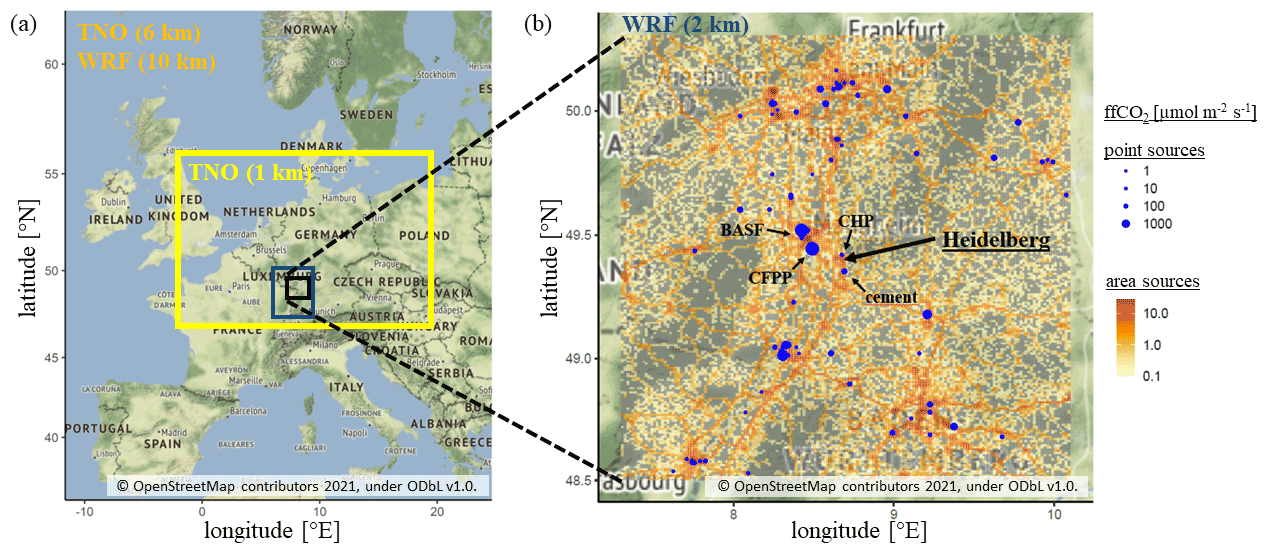
Figure 2(a) Model domain and spatial resolution (in brackets) of nested WRF meteorological fields and TNO emission inventories. In the blue-grey box, TNO has a resolution of about 1 km×1 km and WRF has a resolution of 2 km×2 km. Outside the blue-grey box, the WRF resolution is decreased to 10 km×10 km. Outside the yellow box the TNO inventory has a horizontal resolution of ca. 6 km×6 km. Panel (b) shows a closer view of the Rhine Valley with the TNO area (orange) and point (in blue) source emissions shown (from Super et al., 2020). The observation site Heidelberg and the four closest point sources, i.e. a combined heat and power station (CHP), a cement production facility (cement), a coal-fired power plant (CFPP) and the BASF company in Ludwigshafen, are labelled. The Map tiles are by Stamen Design and used here under CC BY 3.0 (http://maps.stamen.com/terrain/, last access: 4 May 2022). The data are © OpenStreetMap contributors 2021 and distributed under the Open Data Commons Open Database License (ODbL) v1.0.
2.1 Site description
Heidelberg is a medium-sized city with about 160 000 inhabitants located in the Upper Rhine valley in southwestern Germany. It is part of the Rhine–Neckar metropolitan area and includes the heavily industrialised cities of Mannheim (310 000 inhabitants) and Ludwigshafen (170 000 inhabitants) about 15–20 km northwest of Heidelberg. The measurement site is in the northern outskirts of Heidelberg at the Institute of Environmental Physics, which is located on the university campus. There, continuous greenhouse gas measurements and 14CO2 sampling are performed with the sample air intake on the roof of the Institute's building about 30 m above the ground. A more detailed description of the Heidelberg measurement site can be found in Hammer (2008). Figure 2 shows the main ffCO2 point sources in the surroundings of Heidelberg. The largest nearby ffCO2 emitters are the coal-fired power plant in Mannheim, the BASF company in Ludwigshafen, a cement production facility (Heidelberg Zement) south of Heidelberg, and a combined heat and power station about 500 m north of the measurement site.
2.2 Model configuration
We use the coupled Weather Research and Forecasting–Stochastic Time-Inverted Lagrangian Transport model (WRF–STILT) to simulate hourly ffCO2 concentrations for our measurement site in Heidelberg. STILT is a well-established particle dispersion model that uses the mean advection scheme from the Hybrid Single-Particle Lagrangian Integrated Trajectory (HYSPLIT) model (Stein et al., 2015) but with a different representation of turbulence. A detailed description of the WRF–STILT model can be found in Nehrkorn et al. (2010). Hourly ERA5 (European ReAnalysis 5) model estimates at 0.25∘ resolution from the European Centre for Medium-Range Weather Forecasts (ECMWF) are used as input for the WRF model to generate two nested WRF domains. The inner domain covers the Upper Rhine valley with a horizontal resolution of 2 km. The outer domain with a 10 km horizontal resolution includes most of Europe. STILT is driven by these nested WRF fields to calculate hourly back-trajectories for 100 released particles with a maximum backward runtime of 72 h for the Heidelberg observation site. Sensitivity studies with 500 released particles and a maximum backward runtime of 10 d, respectively, showed only minor differences. Thus, we used the mentioned configuration to save computational power for the high-resolution simulations. Highly resolved ffCO2 emission inventories from the Netherlands Organisation for Applied Scientific Research (TNO) are used to describe the European ffCO2 area and point source emissions separately (Super et al., 2020). The area and point source ffCO2 emissions are again divided into 15 different emission source sectors, each with its own temporal (diurnal, weekly and seasonal) profiles. There are two inventories with different horizontal resolutions available, which we nested for this study. The ffCO2 emissions from Germany and its surroundings are resolved on a horizontal grid of about 1 km2 ( longitude × latitude). Emissions from the rest of Europe have a horizontal resolution of . Moreover, TNO provides source sector-specific vertical height profiles for the point source emissions, which we will use for the VSI approach. In the following we explain the mapping of the ffCO2 emissions to the back-trajectories calculated with WRF–STILT.
2.2.1 Surface source influence (SSI) approach
According to Lin et al. (2003) concentration changes ΔC(xr,tr) at the observation site at xr and at time tr can be described by
where S(x,t) describes volume ffCO2 sources (in ppm h−1) and is the influence function for the observation site (with units of m−3), which links the sources to concentration enhancements. The time and volume integration of the influence function can be realised by tallying the total length of time each released particle p spends in a volume element () over time step m (see Lin et al., 2003) and then normalising to the number of released particles Ntot:
Moreover, the volume source S(x,t) can be linked to surface fluxes (in units of mol m−2 s−1) by assuming that turbulent mixing is strong enough to completely mix the surface emissions from the ground into an air column with height h within one model time step m. In STILT, this height h is usually set to half of the planetary boundary layer height hPBL: . Using this method, one receives the following equation:
with the molar mass of air mair and the average air density below h. Inserting Eqs. (2) and (3) into Eq. (1) yields the contribution from each surface grid cell (i,j) and time step m to the total ffCO2 concentration enhancement ΔC(xr,tr) at the observation site:
Here, we call the footprint or surface source influence element, which connects the surface fluxes from grid cell (xi, yj) at time tm to a surface source contribution to the concentration enhancement at the observation site. The sum over all grid cells and times then yields the total concentration enhancement ΔC(xr,tr) at the observation site at xr and time tr.
Fasoli et al. (2018) showed that nearby area sources in the so-called hyper near field (i.e. typically within a distance of less than 10 km) of the observation site are often diluted to only a fraction of the PBLH due to insufficient mixing. Since STILT assumes a complete dilution below this leads to an underestimation of the contribution of the nearby surface fluxes at the observation site. A solution for this is to calculate an effective mixing depth h′ in the hyper near field based on homogeneous turbulence theory (Fasoli et al., 2018; Taylor, 1922), which grows with the distance from the receptor site until it reaches outside the hyper near field. The growth of this effective emission height h′ depends on the meteorological conditions.
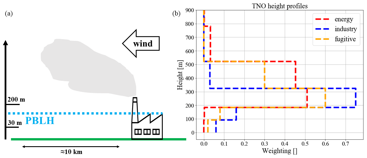
Figure 3(a) Sketch of a possible nocturnal situation when the planetary boundary layer height (PBLH) lies above the measurement height at 30 m a.g.l. but below the exhaust of a nearby power plant stack. (b) TNO height profiles for the public power (energy), industry and fugitive sectors, which were used to calculate the volume influences for the associated point sources. These height profiles are source sector-specific averages, which are representative for Europe.
2.2.2 Volume source influence (VSI) approach
Here, we focus on nearby point source emissions, which are released from stack heights of up to several hundred metres. Handling these nearby point source emissions as surface fluxes will cause errors in the concentration estimates. Consider, for example, a sample collection at 30 m a.g.l. and a 200 m coal power plant exhaust at a distance of about 10 km, which is the situation at our measurement site in Heidelberg (see sketch in Fig. 3a). During typical summer nights with nocturnal inversions, the emissions of the power plant can be above the planetary boundary layer and its influence on the Heidelberg measurements would be very small. But in the surface source influence (SSI) approach, where all emissions from this power plant are mixed into the bottom half of the boundary layer, this will result in large ffCO2 overestimations at the measurement site. To tackle this problem and improve the representation of nearby point source emissions in STILT, we use sector-specific height profiles of the point source emissions from TNO and calculate the so-called volume source influence (VSI) for each height interval. Figure 3b shows the discrete TNO emission height profiles for the relevant point source sectors, i.e. those which are present in the 200 km×200 km area around Heidelberg. These effective emission heights take the stack heights of the point sources as well as subsequent plume rise into account (Kuenen et al., 2022); however, these profiles are source-sector-specific averages, which are representative for Europe. We also used the sector-specific diurnal, weekly and seasonal temporal emission profiles from TNO to consider time-varying area and point source emissions.
The point source fluxes can be distributed into these individual height intervals κ with the TNO sector-specific and height-dependent weighting factors gκ so that the volume source S(x,t) can be expressed for each height interval κ by
For this, we simply assume the molar volume to be constant throughout the different TNO height intervals (from 0 to 1106 m), i.e. , with being the average of the air densities at the particle positions in the air column above (i,j) at time step m. We now can calculate the contribution to the total concentration enhancement at the observation site for each height interval κ by tallying the total length of time each released particle p spends in the volume element () over time step m:
In analogy to the surface source influence, we here call the volume source influence and the volume source contribution to the total concentration enhancement at the observation site.
In this study we used the volume source influence approach to model the contributions from the TNO point sources within a 200 km×200 km box around Heidelberg. All point sources that were further away and the area sources were treated with the surface source approach.
2.3 CO2 sampling for 14C analysis
Since in Heidelberg separate nighttime (from 18:00 to 06:00 UTC) and daytime (from 11:00 to 16:00 UTC) 2-week integrated CO2 samples for 14C analysis are available, the model performance can be investigated separately for night and day. The CO2 sampling technique is described in detail by Levin et al. (1980), and the analysis technique is described by Kromer and Münnich (1992). To estimate regional ffCO2 concentration enhancements from the measured Δ14CO2, the Δ14CO2 signature of background air must be known. Here we use a harmonic fit curve calculated through the Δ14CO2 observations from Mace Head on the western coast of Ireland (MHD, 53∘20′ N, 9∘54′ W, 25 m a.s.l.) and Izaña on Tenerife (IZO, 28∘18′ N, 16∘29′ W, 2400 m a.s.l.), which are both presumably mainly influenced by clean Atlantic air masses (at Mace Head only clean Atlantic air masses are collected for Δ14CO2 analysis). We assume this marine background to be most comparable to the model ffCO2 background, which is set to zero at the border of the model domain (Fig. 2a). Footprint analyses also confirmed that Heidelberg is predominantly influenced by westerly winds and air masses with Atlantic origin. However, for situations with easterly winds and continental air masses from Russia, neither the chosen observational background nor the model background may be fully appropriate. The ffCO2 enhancement cff based on the Heidelberg Δ14CO2 measurements can then be calculated according to
with being the average CO2 concentration in Heidelberg during the 2-week integrated sampling period and Δ14CO2,BG being the Δ14CO2 signature of background air. The Δ14CO2,NUC term describes the contributions from 14CO2 emissions from nuclear facilities and is modelled with the volume source influence approach by assuming that all nuclear 14CO2 emissions are released within a 20 m height interval above a typical stack height of 120 m. In order to avoid interference with our results, we used the VSI approach to calculate the nuclear corrections regardless of whether we later use the VSI or SSI approach for the comparison between modelled and observed ffCO2. To calculate the nuclear corrections, we used the annual mean 14CO2 emissions from the European Commission RAdioactive Discharges Database (RADD, 2021) for the year 2019. We calculated a mean nuclear contribution of and 1.4±0.7 ‰ for the daytime and nighttime samples, respectively. This corresponds to about 7 % of the mean difference between the background and measurement sites for both the daytime and nighttime samples. A detailed derivation of Eq. (7) can be found, e.g. in Levin et al. (2003).
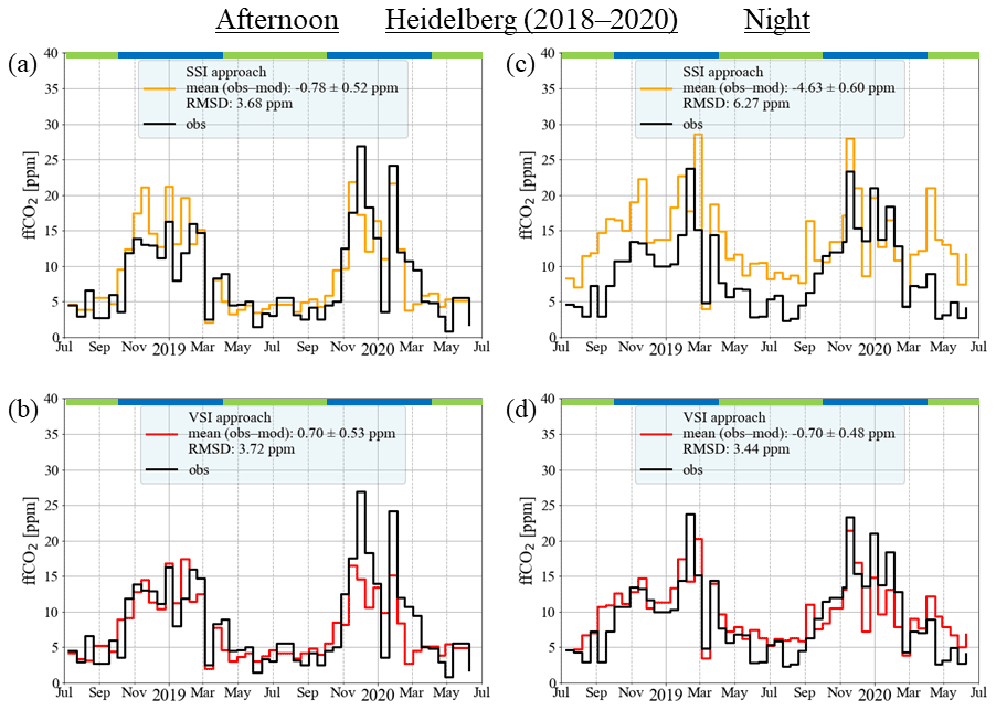
Figure 4Comparison of 2-week integrated 14C-based measured (black) and modelled (coloured) ffCO2 concentration enhancements during afternoon hours (between 11:00 and 16:00 UTC; a and b) and during nighttime (between 18:00 and 06:00 UTC; c and d) for the time period of July 2018 until June 2020 in Heidelberg. The follow two modelling approaches were tested: the standard surface source influence (SSI) approach (orange; a and c) and the volume source influence (VSI) approach (red; b and d); see the text for further details. For each of the comparisons, the root-mean-square deviation (RMSD) between the model and observations, as well as the mean difference (observation minus model) and the standard error of the mean, are given. At the top of each panel the winter and summer periods are marked in blue and green, respectively.
3.1 Comparison of observed and modelled ffCO2 in Heidelberg
In the following section we present the ffCO2 concentrations estimated based on the Heidelberg afternoon and nighttime 2-week integrated samples and compare them to two different WRF–STILT model runs, i.e. the SSI and the VSI approach. Figure 4 shows the measured and modelled 2-week integrated afternoon (left column) and nighttime (right column) ffCO2 enhancements for Heidelberg from July 2018 to June 2020. The black lines show the Δ14CO2 observation-based ffCO2 concentrations calculated using Eq. (7). They represent the ffCO2 enhancement compared to a maritime background introduced in Sect. 2.3. During these 2 years, the 2-week integrated regional ffCO2 concentrations of the afternoon and nighttime samples range from 0.8 to 26.9 and from 2.3 to 23.7 ppm, respectively, with quite similar mean concentrations of 8.2 ppm in the afternoon and 9.0 ppm during the night. Both the afternoon and the nighttime samples show a clear seasonal cycle, with about 3 to 4 times larger ffCO2 concentrations during winter than during summer.
For the afternoon situations, the SSI and the VSI model runs lead to similar root-mean-square deviation (RMSD) between modelled and measured ffCO2 concentrations of 3.7 ppm considered over the whole 2-year period. Whereas the SSI approach leads on average to a small (10 %) overestimation of the ffCO2 concentrations by 0.8 ppm, the VSI approach tends to underestimate ffCO2 by 0.7 ppm (9 %). To put the observed ffCO2 variability and the variability that cannot be explained by the model into perspective, we calculated the coefficient of determination (R2) of linear regression. Both model approaches show similar R2 values of 0.67 (SSI) and 0.63 (VSI) during the afternoon. However, there are seasonal differences in the performance of the two approaches. Whereas both model runs lead to an RMSD between modelled and measured ffCO2 concentrations of 2.0 ppm during the summer half year (from April to September), the RMSD during the winter half year (between October and March) is more than twice as high (4.6 and 4.7 ppm with the SSI approach and the VSI approach, respectively). The worse model performance during winter could be caused by synoptic events with suppressed atmospheric mixing, which frequently occur in winter and are not well represented by transport models. There are, however, differences between the two modelled winters: whereas the VSI approach leads to an improvement compared to the SSI approach during the winter 2018/2019 (RMSD of 2.9 ppm vs. 4.3 ppm), the subsequent winter 2019/2020 shows poorer performance by both modelling approaches (RMSD of 5.9 ppm for the VSI approach and RMSD of 4.9 ppm for the SSI approach).
During nighttime situations we observe large differences between the SSI and VSI approaches. The VSI approach leads to a model–data mismatch comparable to the afternoon situations, with a mean offset between model and observations of −0.7 ppm (8 %) and an RMSD of 3.4 ppm (the RMSD is 3.3 ppm during summertime and 3.6 ppm during wintertime). In contrast, the nighttime SSI run shows by far the largest ffCO2 overestimations throughout the 2 years, with the largest model–observations deviations seen during summer (the RMSD is 6.7 ppm during summertime and 5.8 ppm during wintertime). Over the whole 2 years the average offset is −4.6 ppm (51 %), and the RMSD of 6.3 ppm is almost twice as high as the RMSD of the VSI approach and that of the SSI approach in the afternoon. The poorer SSI performance during the night can also be seen in the R2 values. The VSI approach leads to a R2 of 0.62, which is comparable to the afternoon performance, but the SSI approach shows a lower R2 of 0.48 during the night. To check if the representation of the variability beyond the bias has been improved in the case of the VSI approach, we calculated the bias-corrected (centred) RMSD (CRMSD). It turns out that during the night the SSI approach leads to a CRMSD of 4.2 ppm and the VSI approach leads to a CRMSD of 3.4 ppm. Thus, there is also a slight improvement of the VSI approach in the CRMSD during the night. However, whereas the RMSD is reduced by 46 % in the VSI approach compared to the SSI approach during nighttime, the CRMSD is only reduced by 19 %. This indicates that the VSI approach mainly improves the mean bias between observed and modelled ffCO2 concentrations.

Figure 5Modelled ffCO2 differences between the SSI and VSI approaches for Heidelberg afternoon (blue) and nighttime (red) samples plotted against the modelled mean height of the planetary boundary layer (PBL) during sampling.
We further investigated why the VSI approach is better than the SSI approach during nighttime, whereas both approaches are comparable during afternoon situations. For this we extracted the modelled planetary boundary layer height for Heidelberg from the simulations and averaged it over the nighttime or afternoon times for the full 2 weeks. Figure 5 shows the ffCO2 concentration difference between the SSI and VSI approaches plotted vs. the planetary boundary layer height for all 2-week integrated afternoon (in blue) and nighttime (in red) situations over the 2 years of measurements. During most of the afternoon situations the PBLHs are large, indicating strong convective mixing. The SSI approach with emissions into the bottom half of the PBL then yields similar concentrations at the measurement point as the VSI approach because the VSI height profiles do not (or only slightly) exceed the bottom half of the PBL. On the other hand, low PBLHs result in large concentration differences between the SSI and VSI approaches, which is the case in most of the nighttime and in some afternoon situations between mid-October and February with suppressed convective mixing. During these situations, the SSI approach releases all point source emissions into a shallow layer below the bottom half of the PBL, thus overestimating concentrations at 30 m a.g.l. In contrast, the VSI approach releases emissions at the actual plume height; however, due to the shallow PBL and suppressed convective mixing this leads to only small contributions for an observation site inside the PBL (as is the case for low sampling heights such as at the measurement site in Heidelberg).
3.2 Surface and volume source contributions from nearby point sources in a “pseudo power plant experiment”
Next, we wanted to evaluate if the VSI approach is also relevant for typical continental tall tower stations with elevated sampling heights of, e.g. 200 m a.g.l. For this we conducted a so-called “pseudo power plant experiment”. This experiment should also help determine up to which distance from the measurement site point source emissions should be modelled with the VSI approach to avoid strong overestimations in modelled concentrations during nighttime. Figure 6 shows the aggregated footprints for Heidelberg in 2019, calculated with the SSI approach and our WRF–STILT configuration presented in Sect. 2.2. This mean footprint shows a tail towards the southwestern direction, which can be explained by the channelling effect of the Rhine valley. In our experiment we placed 12 artificial (pseudo) power plants along this footprint tail at distances of 5 to 200 km from Heidelberg, as indicated by the black crosses, so that many situations with contributions from these locations reaching the measurement site in Heidelberg could be expected. All power plants were assigned a CO2 emission rate of 106 t yr−1, which corresponds to typical emissions of small hard coal power plants in Germany (Fraunhofer, 2021). For every hour in 2019, the ffCO2 contribution from each pseudo power plant was modelled with the SSI and VSI approach. In the case of the VSI approach, we used the TNO emission height profile for the public power (energy) sector (see Fig. 3b). We then selected only those hours for which the volume source influence matrix of Heidelberg for a height range between 0 and 1106 m a.g.l. has nonzero entries in each of the 12 pseudo power plant grid cells. By doing so, we have for each pseudo power plant the identical number of selected events (with nonzero contributions) for which we can compare the SSI and the VSI approach. This yields 2060 selected hours in 2019. We then extracted the PBLH at Heidelberg from the WRF–STILT simulation and divided these events into two PBLH regimes (PBLH <500 and PBLH >500 m). The PBLH <500 m situations are predominantly nighttime situations, and those at PBLH >500 m are mainly daytime situations (in 2019, 84 % of the nighttime hours have a PBLH <500 m and 75 % of the daytime situations have a PBLH >500 m).
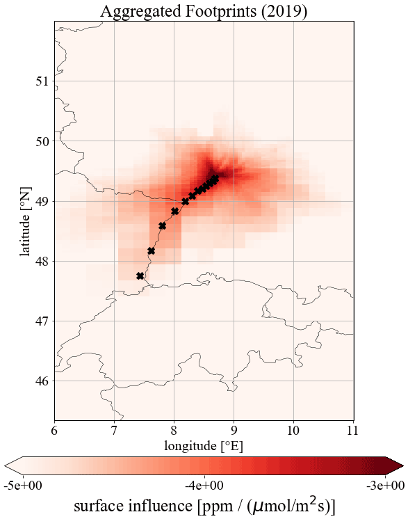
Figure 6Aggregated hourly footprints in 2019, calculated with the SSI approach for the observation site Heidelberg at 30 m height a.g.l. The black crosses indicate the locations of the 12 pseudo power plants, which are located at distances of 5, 10, 15, 20, 25, 30, 40, 50, 70, 100, 150 and 200 km from the Heidelberg observation site.

Figure 7Mean ffCO2 contributions from pseudo power plants, which were placed at distances between 5 and 200 km from the observation site Heidelberg at 30 m (a–c) and at a virtual 200 m height (d–f). Shown are the results from the SSI (a and d) and VSI approach when using the TNO public power (energy) profile (b and e), as well as the mean difference between the SSI and VSI ffCO2 contributions (c and f). From all hours in 2019, only those situations were selected for which each pseudo power plant grid cell is hit by at least 1 of the 100 back-trajectories, which were calculated for each hour. These selected hours are then divided into two planetary boundary layer height (PBLH) regimes (blue and red) and averaged. For this, we always used the PBLH at the Heidelberg measurement site at the time when the air parcels from the power plants arrived in Heidelberg. In (f), negative values are indicated with red (PBLH <500 m) and blue (PBLH >500 m) arrows.
Figure 7a (7b) shows the mean ffCO2 contributions from the individual pseudo power plants vs. their distances from Heidelberg when the SSI (VSI) approach is used. Events were separated into situations when the PBLH in Heidelberg was smaller than 500 m (red dots) or larger than 500 m (blue dots). The mean ffCO2 contribution differences between the SSI and VSI approach (SSI minus VSI) for the individual pseudo power plants are shown in Fig. 7c. It is obvious that the mean ffCO2 contributions from the power plants decrease with increasing distance from the observation site in both modelling approaches. This can be explained by the dispersion of the power plant plumes and the associated dilution. To restrict the mean ffCO2 contribution from these power plants to below 0.1 ppm, the observation site should be more than 100 km (SSI) or 50 km (VSI) away from this power plant. This is in line with the ICOS recommendations that suggest a distance of at least 40 km from strong anthropogenic sources (ICOS RI, 2020). Figure 7a shows that the SSI approach yields larger contributions for stable PBLH <500 m situations compared to (daytime) situations with PBLH >500 m. Since in the SSI approach the emissions are homogeneously mixed into the bottom half of the PBL, the smaller mixing volume during PBLH <500 m situations leads to larger ffCO2 concentrations. This is what we have already seen from our daytime and nighttime simulations of real-world ffCO2 (see Fig. 5). The reduction of the ffCO2 contributions with increasing PBLH could be seen as an increased vertical dispersion of the power plant plumes. In the “pseudo power plant experiment” the VSI approach shows the same behaviour as the SSI approach with larger ffCO2 contributions during stable PBLH <500 m situations for most power plants, which can also be explained by less dispersion of the power plant plumes. However, there is one exception in the VSI approach. The power plant with a 5 km distance yields lower ffCO2 contributions during stable PBLH <500 m conditions than during PBLH >500 m situations (in contrast to the SSI approach). A possible explanation is that during stable PBL conditions the mixing is too weak to transport the emissions from the power plant stack down to the sampling height at 30 m within the time the air mass needs to travel the 5 km from the power plant to the observation site (see Fasoli et al., 2018).
Looking at the mean ffCO2 contribution differences (Fig. 7c) between the two model approaches reveals that for the 30 m high observation site the SSI approach simulates almost 5 ppm larger ffCO2 contributions on average than the VSI approach for the closest (5 km distance) power plant during stable conditions. This can be explained by (i) the large SSI contributions due to the shallow boundary layer and (ii) the low VSI contributions due to suppressed downward mixing of the power plant plume to the 30 m high observation site. During PBLH >500 m situations and for more distant power plants the mean difference between the SSI and VSI contributions decreases due to stronger mixing or more time for mixing over the longer air mass travel time between the power plant and observation site. In both cases, the assumption in the SSI approach, i.e. an instantaneous and homogeneous dilution of all power plant emissions in the bottom half of the PBL, seems to be more justified than during PBLH <500 m situations and for power plants very close to the measurement site. Further, the difference between PBLH <500 m and PBLH >500 m situations decreases with distance to the power plants. One reason for this could be that, due to the longer travel time (e.g. >12 h for the furthest power plant during wind velocities of <5 m s−1), a power plant plume arriving at nighttime in Heidelberg was still well mixed over a large boundary layer during the previous day.
Since ICOS tower stations have most of their air inlets above 30 m a.g.l. (typically between 30 and 250 m), we also investigated the behaviour of the SSI and VSI approach for a virtual Heidelberg sampling height at 200 m a.g.l. The results are shown in Fig. 7d–f. In contrast to the 30 m air inlet, for the 200 m air inlet the SSI approach shows less enhancements compared to the VSI approach during stable conditions and for power plants very close by. Whereas for example the closest 5 km distant power plant leads to an SSI minus VSI ffCO2 difference of 4.9 ppm in the case of the 30 m air inlet, this difference is reduced to 0.6 ppm in the case of the 200 m air inlet. This means that the SSI contribution in the case of the 30 m air inlet is 17.4 times larger than the VSI contribution. In the case of the 200 m air inlet, the SSI contribution from the closest power plant is only 1.8 times larger during PBLH <500 m situations. This could be explained by situations with very stable conditions (with for PBLH <200 m), when the sampling height at 200 m a.g.l. is above the PBL and hardly sensitive to emissions that are mixed within the bottom half of the PBL (in the SSI approach). In contrast, the VSI approach yields larger ffCO2 contributions from nearby power plants compared to the case with the 30 m sampling height, since the sampling height (200 m a.g.l.) is now closer to the effective emission height. Consequently, the 200 m sampling height shows (in contrast to the 30 m sampling height) on average lower ffCO2 contribution differences between SSI and VSI approach, especially for contributions from very close power plants and during stable PBL situations.
4.1 Effects of emission uncertainties on the comparison between observed and modelled ffCO2 in Heidelberg
The model–data mismatch presented in Fig. 4 depends not only on the representation of atmospheric transport and the handling of point source emissions but also on uncertainties in the emission inventory. Since we interpret the model–data mismatch difference for the evaluation of the SSI and VSI approach, we need to ensure that it is not caused by incorrect area or point source distribution or temporal profiles in the emission inventory. If, for example, the nocturnal point source emissions were overestimated in the inventory, we would consider the VSI approach to yield better agreement with observations for the wrong reason. Therefore, we first want to discuss uncertainties in the inventory and assess which theoretical overestimation in the inventory would be needed to generate the apparent improvement of the model–data mismatch going from SSI to the VSI approach. Super et al. (2020) identified four sources of uncertainties in the high-resolution TNO inventory: (1) uncertainties in the national activity data, (2) uncertainties in the emission factors, which quantify the ffCO2 emissions that are released per unit of activity and are related to the carbon content of the fuels, (3) uncertainties in the spatial distribution of the national emissions, which rely on spatial proxies like population or traffic density and finally (4) uncertainties in the temporal profiles of emissions. Super et al. (2020) used a Monte Carlo approach to produce 10 high-resolution TNO inventory ensembles for the annual emissions in 2015 by incorporating uncertainties (1) to (3) for the area sources. They regard the point source emission uncertainties as quite low and thus excluded them from the Monte Carlo simulations. For a 200 km×200 km area around Heidelberg, the annual total ffCO2 area source emission calculated from the 10 emission grid realisations spreads by about ±3 %. Based on the results of Super et al. (2020), we may thus assume a very low uncertainty for the area and point sources, which could not explain the observed differences in the model–data mismatch between SSI and VSI.
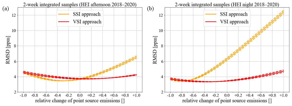
Figure 8Root-mean-square deviation (RMSD) between measured and modelled ffCO2 concentrations of 2-week integrated afternoon (a) and nighttime (b) Δ14CO2 samples collected during July 2018 and June 2020 in Heidelberg (HEI) at 30 m a.g.l. for the surface (SSI, in orange) and volume source influence (VSI, in red) approaches for different relative changes in the TNO point source emissions. A relative change of −1 means that all point source emissions are switched off, and a relative change of +1 means that the actual emissions of all point sources are doubled. For instance, the actual point source emissions would have to be decreased by about 70 % (corresponds to −0.7 on the x axis), and thus SSI and VSI approach lead to a similar RMSD for nighttime situations. The dashed lines show the additional impact of a TNO area source emission uncertainty of ±3 % (see Super et al., 2020) on the RMSD between measured and modelled ffCO2 concentrations.
In a thought experiment we tested how much we would have to change the actual point source emissions so that SSI and VSI approach lead to a similarly good agreement with observations during nighttime. In Fig. 8 we show that the point source emissions would have to be reduced by as much as 70 % during nighttime to show a similar model–data mismatch for the SSI approach to that of the VSI approach. Such large point source emission uncertainties are unrealistic and unexpected. Based on these considerations, we conclude that it is highly unlikely that the improved model–data mismatch of the nocturnal VSI approach is due to biases in the temporal profile of the emissions. The improvement in the VSI approach can therefore be attributed to the different vertical representation of the point sources.
4.2 Representation of nearby point source emissions in models
Typically, flask samples for model–observation comparisons or inversions are collected in the afternoon during well-mixed conditions when the atmospheric transport and mixing processes can be best simulated (Geels et al., 2007). However, the inclusion of nighttime observations into inversion modelling frameworks would drastically increase the number of observational data that could be used to optimise emissions and could help draw conclusions about the mixture and the diurnal emission profiles of source sectors that are more active during night or in the morning and evening hours. The exploitation of nighttime observations in inverse modelling studies relies on the model's ability to realistically reproduce stable nocturnal boundary layers. Here, we discuss the effect of point source emission heights on the model–data mismatch, especially during nighttime, and assess when and where the volume source influence approach should be applied.
The pseudo power plant experiment yields a mean SSI minus VSI contribution difference between about 0.5 ppm (for a 15 km distant power plant) and 4.9 ppm (for a 5 km distant power plant) during stable conditions with low PBLHs. Since the Heidelberg measurement site is surrounded by several point sources, some of them emitting more than 106 t CO2 yr−1 (see Fig. 2), we decided to apply the VSI approach to all point sources within a 200 km×200 km area around Heidelberg and use the SSI approach for the point sources further away, where we expect only small differences between the VSI and SSI approach. The ffCO2 results for the 2-week integrated nighttime samples showed that the model–data mismatch could already be reduced by about 3 ppm (RMSD =3.4 ppm) when using this VSI approach for nearby point sources instead of the standard SSI approach (RMSD =6.3 ppm). During well-mixed conditions the pseudo power plant experiment showed smaller differences between the VSI and SSI approach, which can also be seen in the ffCO2 results for the 2-week integrated afternoon samples, where the VSI approach and the SSI approach differ by merely ca. 1 % (both approaches lead to an RMSD of about 3.7 ppm). Thus, we strongly recommend the application of the VSI approach for measurement sites with sampling heights typically within the nocturnal boundary layer and with nearby point sources so that also nighttime observations could be used, e.g. for a model–observation comparison. However, the VSI approach is accompanied by larger computational costs since the volume influence field v must be calculated for each height interval. In contrast, in the SSI approach only one surface influence field f must be calculated (see Sect. 2.2). To save computational power we therefore suggest that the VSI approach only be used for nearby point sources and to use the SSI approach for more distant point sources where both model approaches lead to similar results. Depending on the distribution and the emission strength of the point sources around the measurement site and the intake height of the measurement site, the results from the pseudo power plant experiment can help to decide for which point sources the VSI approach should be applied. From this experiment it follows that the SSI minus VSI differences are substantial for low intake heights (e.g. 30 m) and power plants within a radius of 5 to 15 km. When averaged over the two PBLH regimes (<500 and >500 m), these differences come to 3.9 and 0.5 ppm respectively, equivalent to a 12- or 2-fold increase in the absolute VSI contribution for a point source emitting 1 MtCO2 yr−1. Such a station and point source configuration is realistic for urban observations. For ICOS-like background stations, which should typically be located 50 km from point sources, the SSI minus VSI difference is less than 0.1 ppm and thus even less than the World Meteorological Organization (WMO) compatibility goal for CO2 (WMO, 2018).
Since the 14CO2 samples are collected at many ICOS stations from a higher intake, we performed the pseudo power plant experiment also for a (virtual) Heidelberg observation site at 200 m a.g.l. (where we do not have real measurements). The results show that for nearby power plants the mean SSI minus VSI contribution differences are roughly an order of magnitude smaller than in the case of the observation site at 30 m a.g.l. However, one has to keep in mind that although the SSI minus VSI contribution differences are smaller in the case of the 200 m high observation site, the SSI approach does not represent the atmospheric transport processes any better than in the case of the observation site at 30 m a.g.l. It simply means that the 200 m intake height is less sensitive to the bottom half of the PBL during stable conditions, which leads to less overestimations for the SSI compared to the VSI approach. The randomness of the SSI contributions becomes immediately clear if one considers the 15 and 20 km distant power plant. Here, the SSI approach yields even smaller contributions than the VSI approach during stable conditions. Moreover, the 200 m intake height is vertically closer to the effective emission height of the power plants, which leads to larger VSI contributions compared to the 30 m level. These two circumstances cause the smaller mean SSI minus VSI contribution differences for nearby point sources in the case of the 200 m level. The mean SSI minus VSI contribution difference for a 106 t CO2 yr−1 emitting point source is below 0.1 ppm if the point source is at least 10 km away from the measurement site. However, one has to keep in mind that this absolute difference in SSI minus VSI contribution increases linearly with the emission strength of the point sources. Thus, for ICOS-like stations and point sources at least 10 km away, the SSI approach again seems to be well suited when there is enough time for mixing throughout the PBL and the SSI assumptions are justified.
Inaccurate representation of point source emissions from stacks is not limited to Lagrangian models but is found in many Eulerian modelling setups as well. Super et al. (2017) investigated how well a Eulerian model (WRF–Chem) alone, as well as in combination with a Gaussian plume model, agrees with CO2 and CO mixing ratios at an urban site in the Netherlands. In the case of the Eulerian model, the point source emissions are distributed over the different vertical model levels according to the emission height profiles shown in Fig. 3, which is rather similar to the VSI approach we used in WRF–STILT. The Gaussian plume model is able to represent the exact emission stack heights and improves the description of the transport and dispersion of the point source plumes, which in the case of Eulerian models are instantly mixed within individual grid boxes (Super et al., 2017). The authors could show that both the exact representation of the stack heights and the more appropriate description of the plume dispersion will lead to a better agreement to the observations in the case of the WRF–Chem model in combination with the Gaussian plume model. Therefore, they recommend to treat all large point source emissions within a 10 km radius around the observation site with such a plume model.
In this study we used a 2-year record of afternoon and nighttime 2-week integrated 14C-based ffCO2 measurements conducted in Heidelberg at 30 m a.g.l. to examine the performance of the standard STILT surface source influence (SSI) approach. We find that it is almost twice as good for afternoon situations (RMSD =3.7 ppm) than for the nighttime situations (RMSD =6.3 ppm) when comparing modelled and observed ffCO2 concentrations. The lower performance during the night could be explained by the large overestimation of the contributions from nearby point sources. We therefore introduced an alternative modelling approach – the volume source influence (VSI) approach – which is able to represent the emission height and the plume rise of the point source emissions more correctly. With this approach, the performance of STILT is similar for the afternoon (RMSD =3.7 ppm) and nighttime samples (RMSD =3.4 ppm).
We further investigated the behaviour of the SSI and VSI approach for point sources at different distances to the measurement site and under different atmospheric conditions. For this we performed a pseudo power plant experiment by modelling the ffCO2 contributions from 12 virtual power plants with distances between 5 and 200 km from the observation site and annual emissions of one million tonnes of CO2. This model experiment could confirm what we already observed in the model–observation comparison of the 2-week integrated samples, namely that the standard SSI approach leads to strong overestimations compared to the VSI approach given stable atmospheric conditions with low planetary boundary layer heights, especially for point sources close to the observation site. For instance, point sources with a distance between 5 and 15 km from the observation site lead to a mean SSI minus VSI difference of 3.9 to 0.5 ppm ffCO2, which is 12 to 2 times larger than the mean VSI ffCO2 contribution from these point sources. Thus, we strongly recommend the use of the VSI approach for these close-by point sources when modelling their ffCO2 contribution at low-altitude measurement sites. For ICOS-like background stations, which should typically be located more than 50 km away from point sources, the mean SSI minus VSI difference reduces to below 0.1 ppm. We also performed this model experiment for a virtual observation site with a 200 m sampling height, which is more comparable to the uppermost measurement height of typical ICOS stations. Here, the mean contribution differences between the SSI and VSI approaches for nearby point sources are smaller compared to those at the 30 m sampling height because the 200 m height is less sensitive to the bottom half of the PBL during very stable situations (leading to smaller SSI contributions) and is vertically closer to the effective power plant emission height (leading to larger VSI contributions). Whereas for low sampling heights the VSI approach is strongly recommended to model contributions from nearby point sources in order to avoid large overestimations (on the order of several parts per million for ffCO2) during stable conditions, we also suggest the use of the VSI approach in the case of sampling heights well above the nocturnal boundary layer since it is the physically more correct approach for these situations with suppressed mixing. The contributions from more distant point sources are generally smaller and also the assumptions in the SSI approach seem to be more justified for longer air mass travel times between the point source and observation site and during unstable atmospheric conditions. This explains the smaller differences between the SSI and VSI approach for these situations. Depending on the atmospheric conditions, the sampling height, the distance to the point source and the emission strength of the point source, the results of our pseudo power plant experiment can be used to assess the contribution of the point source in both modelling approaches. Then one can decide if the SSI approach is sufficient (e.g. for distant point sources with lower emissions or during unstable conditions) or if the VSI approach is the better alternative.
Whereas the modelling of transport and mixing processes is still challenging during nighttime, we showed with this study that using the VSI approach for nearby point sources will greatly reduce the overestimations of contributions from nearby point source emissions during periods with low PBLH, especially for low-altitude measurement sites. Therefore, this approach could possibly be a first step towards the usage of nighttime observations for modelling purposes in STILT. A further inevitable step towards the exploitation of nighttime observations in models is the realistic representation of stable nocturnal boundary layers and their erosion in the morning hours. Moreover, we want to underline the importance of having an inventory containing the effective point source emission heights for the whole globe, which is a prerequisite for applying this VSI approach also outside Europe.
The measurement and model results for the 2-week integrated samples collected at Heidelberg and the outcome of the pseudo power plant experiment are available at the Heidelberg University data depository (https://doi.org/10.11588/data/CK3ZTX, Maier et al., 2021). The R script (“volume.infl.ffco2.timeres.r”) to calculate ffCO2 contributions from point sources and the used trajectory information calculated with WRF–STILT and the TNO point source emissions around Heidelberg can be found at https://doi.org/10.5281/zenodo.5911518 (Maier et al., 2022). To calculate the trajectories for other locations or times, one has to download the full STILT model, which is available at http://stilt-model.org/ (last access: 7 July 2022, Lin et al., 2003) after registration. We used revision number 747 of the STILT repository.
FM designed the study together with CG, IL and SH. FM performed the STILT modelling and evaluated the data. CG helped with the implementation of STILT. SH compiled the measurement results of the 2-week integrated 14CO2 samples. IS was responsible for the TNO emission inventories. JM generated the highly resolved meteorological fields with WRF. FM wrote the manuscript with help of all co-authors.
The contact author has declared that none of the authors has any competing interests.
Publisher's note: Copernicus Publications remains neutral with regard to jurisdictional claims in published maps and institutional affiliations.
We would like to thank Sharon Gourdji and the anonymous reviewer for their inspiring comments and suggestions, which helped to improve the paper. We gratefully acknowledge Thomas Koch and Michał Gałkowski for their help with running STILT. We wish to thank the staff of TNO at the Department of Climate, Air and Sustainability in Utrecht for the emission inventories and height profiles. A special thank goes to Sabine Kühr and the whole staff of the ICOS-CRL Karl Otto Münnich Laboratory for their careful 14CO2 sampling and analysis and to Julian Della Coletta and the ICOS Atmospheric Thematic Centre for conducting and evaluating the continuous CO2 measurements in Heidelberg. We further would like to thank Ida Storm and the members of the ICOS Carbon Portal for their cooperation in developing tools for estimating nuclear 14CO2 contamination at European ICOS stations.
This research has been supported by the German Weather Service (DWD), the ICOS Research Infrastructure and VERIFY (grant no. 776810, Horizon 2020 Framework). The ICOS Central Radiocarbon Laboratory is funded by the German Federal Ministry of Transport and Digital Infrastructure. Fabian Maier was paid by the DWD.
This paper was edited by Christoph Knote and reviewed by Sharon Gourdji and one anonymous referee.
Basu, S., Miller, J. B., and Lehman, S.: Separation of biospheric and fossil fuel fluxes of CO2 by atmospheric inversion of CO2 and 14CO2 measurements: Observation System Simulations, Atmos. Chem. Phys., 16, 5665–5683, https://doi.org/10.5194/acp-16-5665-2016, 2016.
Basu, S., Lehman, S. J., Miller, J. B., Andrews, A. E., Sweeney, C., Gurney, K. R., Xue, X., Southon, J., and Tans, P. P.: Estimating US fossil fuel CO2 emissions from measurements of 14C in atmospheric CO2, P. Natl. Acad. Sci. USA, 117, 13300–13307, https://doi.org/10.1073/pnas.1919032117, 2020.
Brunner, D., Kuhlmann, G., Marshall, J., Clément, V., Fuhrer, O., Broquet, G., Löscher, A., and Meijer, Y.: Accounting for the vertical distribution of emissions in atmospheric CO2 simulations, Atmos. Chem. Phys., 19, 4541–4559, https://doi.org/10.5194/acp-19-4541-2019, 2019.
Currie, L. A.: The remarkable metrological history of radiocarbon dating [II], J. Res. Natl. Inst. Stan., 109, 185–217, https://doi.org/10.6028/jres.109.013, 2004.
Fasoli, B., Lin, J. C., Bowling, D. R., Mitchell, L., and Mendoza, D.: Simulating atmospheric tracer concentrations for spatially distributed receptors: updates to the Stochastic Time-Inverted Lagrangian Transport model's R interface (STILT-R version 2), Geosci. Model Dev., 11, 2813–2824, https://doi.org/10.5194/gmd-11-2813-2018, 2018.
Fraunhofer: Fraunhofer-Institut für Solare Energiesysteme ISE, Energy-Charts, https://energy-charts.info/charts/emissions/chart.htm?l=de&c=DE&source=hard_coal, last access: 6 August 2021.
Friedlingstein, P., O'Sullivan, M., Jones, M. W., Andrew, R. M., Hauck, J., Olsen, A., Peters, G. P., Peters, W., Pongratz, J., Sitch, S., Le Quéré, C., Canadell, J. G., Ciais, P., Jackson, R. B., Alin, S., Aragão, L. E. O. C., Arneth, A., Arora, V., Bates, N. R., Becker, M., Benoit-Cattin, A., Bittig, H. C., Bopp, L., Bultan, S., Chandra, N., Chevallier, F., Chini, L. P., Evans, W., Florentie, L., Forster, P. M., Gasser, T., Gehlen, M., Gilfillan, D., Gkritzalis, T., Gregor, L., Gruber, N., Harris, I., Hartung, K., Haverd, V., Houghton, R. A., Ilyina, T., Jain, A. K., Joetzjer, E., Kadono, K., Kato, E., Kitidis, V., Korsbakken, J. I., Landschützer, P., Lefèvre, N., Lenton, A., Lienert, S., Liu, Z., Lombardozzi, D., Marland, G., Metzl, N., Munro, D. R., Nabel, J. E. M. S., Nakaoka, S.-I., Niwa, Y., O'Brien, K., Ono, T., Palmer, P. I., Pierrot, D., Poulter, B., Resplandy, L., Robertson, E., Rödenbeck, C., Schwinger, J., Séférian, R., Skjelvan, I., Smith, A. J. P., Sutton, A. J., Tanhua, T., Tans, P. P., Tian, H., Tilbrook, B., van der Werf, G., Vuichard, N., Walker, A. P., Wanninkhof, R., Watson, A. J., Willis, D., Wiltshire, A. J., Yuan, W., Yue, X., and Zaehle, S.: Global Carbon Budget 2020, Earth Syst. Sci. Data, 12, 3269–3340, https://doi.org/10.5194/essd-12-3269-2020, 2020.
Geels, C., Gloor, M., Ciais, P., Bousquet, P., Peylin, P., Vermeulen, A. T., Dargaville, R., Aalto, T., Brandt, J., Christensen, J. H., Frohn, L. M., Haszpra, L., Karstens, U., Rödenbeck, C., Ramonet, M., Carboni, G., and Santaguida, R.: Comparing atmospheric transport models for future regional inversions over Europe – Part 1: mapping the atmospheric CO2 signals, Atmos. Chem. Phys., 7, 3461–3479, https://doi.org/10.5194/acp-7-3461-2007, 2007.
Gerbig, C., Körner, S., and Lin, J. C.: Vertical mixing in atmospheric tracer transport models: error characterization and propagation, Atmos. Chem. Phys., 8, 591–602, https://doi.org/10.5194/acp-8-591-2008, 2008.
Hammer, S.: Quantification of the regional H2 sources and sinks inferred from atmospheric trace gas variability, PhD Thesis, University of Heidelberg, 2008.
Heiskanen, J., Brümmer, C., Buchmann, N., Calfapietra, C., Chen, H., Gielen, B., Gkritzalis, T., Hammer, S., Hartman, S., Herbst, M., Janssens, I. A., Jordan, A., Juurola, E., Karstens, U., Kasurinen, V., Kruijt, B., Lankreijer, H., Levin, I., Linderson, M., Loustau, D., Merbold, L., Myhre, C. L., Papale, D., Pavelka, M., Pilegaard, K., Ramonet, M., Rebmann, C., Rinne, J., Rivier, L., Saltikoff, E., Sanders, R., Steinbacher, M., Steinhoff, T., Watson, A., Vermeulen, A. T., Vesala, T., Vítková, G., and Kutsch, W.: The Integrated Carbon Observation System in Europe, B. Am. Meteorol. Soc., 103, E855–E872, https://doi.org/10.1175/BAMS-D-19-0364.1, 2022.
ICOS RI: ICOS Atmosphere Station Specifications V2.0, edited by: Laurent, O., ICOS ERIC, https://doi.org/10.18160/GK28-2188, 2020.
Kromer, B. and Münnich, K. O.: CO2 gas proportional counting in radiocarbon dating – review and perspective, in: Radiocarbon after four decades, edited by: Taylor, R. E., Long, A., and Kra, R. S., Springer, New York, 184–197, https://doi.org/10.1007/978-1-4757-4249-7_13, 1992.
Kuenen, J., Dellaert, S., Visschedijk, A., Jalkanen, J.-P., Super, I., and Denier van der Gon, H.: CAMS-REG-v4: a state-of-the-art high-resolution European emission inventory for air quality modelling, Earth Syst. Sci. Data, 14, 491–515, https://doi.org/10.5194/essd-14-491-2022, 2022.
Levin, I., Münnich, K. O., and Weiss, W.: The Effect of Anthropogenic CO2 and 14C Sources on the Distribution of 14C in the Atmosphere, Radiocarbon, 22, 379–391, https://doi.org/10.1017/S003382220000967X, 1980.
Levin, I., Kromer, B., Schmidt, M., and Sartorius, H.: A novel approach for independent budgeting of fossil fuel CO2 over Europe by 14CO2 observations, Geophys. Res. Lett., 30, 2194, https://doi.org/10.1029/2003GL018477, 2003.
Levin, I., Hammer, S., Kromer, B., and Meinhardt, F.: Radiocarbon observations in atmospheric CO2: determining fossil fuel CO2 over Europe using Jungfraujoch observations as background, Sci. Total Environ., 391, 211–216, https://doi.org/10.1016/j.scitotenv.2007.10.019, 2008.
Levin, I., Karstens, U., Eritt, M., Maier, F., Arnold, S., Rzesanke, D., Hammer, S., Ramonet, M., Vítková, G., Conil, S., Heliasz, M., Kubistin, D., and Lindauer, M.: A dedicated flask sampling strategy developed for Integrated Carbon Observation System (ICOS) stations based on CO2 and CO measurements and Stochastic Time-Inverted Lagrangian Transport (STILT) footprint modelling, Atmos. Chem. Phys., 20, 11161–11180, https://doi.org/10.5194/acp-20-11161-2020, 2020.
Lin, J. C., Gerbig, C., Wofsy, S. C., Andrews, A. E., Daube, B. C., Davis, K. J., and Grainger, C. A.: A near-field tool for simulating the upstream influence of atmospheric observations: The Stochastic Time-Inverted Lagrangian Transport (STILT) model, J. Geophys. Res., 108, 4493, https://doi.org/10.1029/2002JD003161, 2003 (data available at: http://stilt-model.org/, last access: 7/ July 2022).
Maier, F., Gerbig, C., Levin, I., Super, I., Marshall, J., and Hammer, S.: Heidelberg integrated samples 2018–2020 and pseudo power plant experiment results, Heidelberg University – Institute of Environmental Physics, heiData [data set], https://doi.org/10.11588/data/CK3ZTX, 2021.
Maier, F., Gerbig, C., and Koch, T. F.: Calculating ffCO2 contributions from nearby point sources with STILT surface source and volume source influence approach, Zenodo, https://doi.org/10.5281/zenodo.5911518, 2022.
Nehrkorn, T., Eluszkiewicz, J., Wofsy, S. C., Lin, J. C., Gerbig, C., Longo, M., and Freitas, S.: Coupled weather research and forecasting–stochastic time-inverted lagrangian transport (WRF–STILT) model, Meteorol. Atmos. Phys., 107, 51–64, https://doi.org/10.1007/s00703-010-0068-x, 2010.
RADD: European Commission RAdioactive Discharges Database, https://europa.eu/radd/query.dox?pageID=Query, last access: 8 June 2021.
Stein, A. F., Draxler, R. R., Rolph, G. D., Stunder, B. J. B., Cohen, M. D., and Ngan, F.: NOAA's HYSPLIT Atmospheric Transport and Dispersion Modeling System, B. Am. Meteorol. Soc., 96, 2059–2077, https://doi.org/10.1175/BAMS-D-14-00110.1, 2015.
Super, I., Denier van der Gon, H. A. C., van der Molen, M. K., Sterk, H. A. M., Hensen, A., and Peters, W.: A multi-model approach to monitor emissions of CO2 and CO from an urban–industrial complex, Atmos. Chem. Phys., 17, 13297–13316, https://doi.org/10.5194/acp-17-13297-2017, 2017.
Super, I., Dellaert, S. N. C., Visschedijk, A. J. H., and Denier van der Gon, H. A. C.: Uncertainty analysis of a European high-resolution emission inventory of CO2 and CO to support inverse modelling and network design, Atmos. Chem. Phys., 20, 1795–1816, https://doi.org/10.5194/acp-20-1795-2020, 2020.
Super, I., Dellaert, S. N. C., Tokaya, J. P., and Schaap, M.: The impact of temporal variability in prior emissions on the optimization of urban anthropogenic emissions of CO2, CH4 and CO using in-situ observations, Atmos. Environ., 11, 100119, https://doi.org/10.1016/j.aeaoa.2021.100119, 2021.
Taylor, G. I.: Diffusion by continuous movements, P. Lond. Mathe. Soc., s2–20, 196–212, https://doi.org/10.1112/plms/s2-20.1.196, 1922.
Turnbull, J. C., Sweeney, C., Karion, A., Newberger, T., Lehman, S. J., Tans, P. P., Davis, K. J., Lauvaux, T., Miles, N. L., Richardson, S. J., Cambaliza, M. O., Shepson, P. B., Gurney, K., Patarasuk, R., and Razlivanov, I.: Toward quantification and source sector identification of fossil fuel CO2 emissions from an urban area: Results from the INFLUX experiment, J. Geophys. Res.-Atmos., 120, 292–312, https://doi.org/10.1002/2014JD022555, 2015.
Wang, Y., Broquet, G., Ciais, P., Chevallier, F., Vogel, F., Wu, L., Yin, Y., Wang, R., and Tao, S.: Potential of European 14CO2 observation network to estimate the fossil fuel CO2 emissions via atmospheric inversions, Atmos. Chem. Phys., 18, 4229–4250, https://doi.org/10.5194/acp-18-4229-2018, 2018.
Wenger, A., Pugsley, K., O'Doherty, S., Rigby, M., Manning, A. J., Lunt, M. F., and White, E. D.: Atmospheric radiocarbon measurements to quantify CO2 emissions in the UK from 2014 to 2015, Atmos. Chem. Phys., 19, 14057–14070, https://doi.org/10.5194/acp-19-14057-2019, 2019.
WMO: GAW Report No. 242, 19th WMO/IAEA Meeting on Carbon Dioxide, Other Greenhouse Gases and Related Tracers Measurement Techniques (GGMT-2017), edited by: Crotwell, A. and Steinbacher, M., World Meteorological Organization, Geneva, Dübendorf, Switzerland, 27–31 August 2017, https://library.wmo.int/doc_num.php?explnum_id=5456 (last access: 7 July 2022), 2018.