the Creative Commons Attribution 4.0 License.
the Creative Commons Attribution 4.0 License.
 | 07 Jul 2022
Computation of longwave radiative flux and vertical heating rate with 4A-Flux v1.0 as an integral part of the radiative transfer code 4A/OP v1.5
Cyril Crevoisier
Raymond Armante
Jean-Louis Dufresne
Nicolas Meilhac
Based on advanced spectroscopic databases, line-by-line and layer-by-layer radiative transfer codes numerically solve the radiative transfer equation with very high accuracy. Taking advantage of its pre-calculated optical depth lookup table, the fast and accurate radiative transfer model Automatized Atmospheric Absorption Atlas OPerational (4A/OP) calculates the transmission and radiance spectra for a user-defined layered atmospheric model. Here, we present a module called 4A-Flux, which is developed and implemented into 4A/OP in order to include the calculation of the clear-sky longwave radiative flux profiles and heating rate profiles at a very high spectral resolution. Calculations are performed under the assumption of local thermodynamic equilibrium, a plane-parallel atmosphere, and specular reflection on the surface. The computation takes advantage of pre-tabulated exponential integral functions that are used instead of a classic angular quadrature. Furthermore, the sub-layer variation of the Planck function is implemented to better represent the emission of layers with a high optical depth. Thanks to the implementation of 4A-Flux, 4A/OP models have participated in the Radiative Forcing Model Intercomparison Project (RFMIP-IRF) along with other state-of-the-art radiative transfer models. 4A/OP hemispheric flux profiles are compared to other models over the 1800 representative atmospheric situations of RFMIP, yielding an outgoing longwave radiation (OLR) mean difference between 4A/OP and other models of −0.148 W m−2 and a standard deviation of 0.218 W m−2, showing a good agreement between 4A/OP and other models. 4A/OP is applied to the Thermodynamic Initial Guess Retrieval (TIGR) atmospheric database to analyze the response of the OLR and vertical heating rate to several perturbations of temperature or gas concentration. This work shows that 4A/OP with 4A-Flux module can successfully be used to simulate accurate flux and heating rate profiles and provide useful sensitivity studies including sensitivities to minor trace gases such as HFC134a, HCFC22, and CFC113. We also highlight the interest for the modeling community to extend intercomparison between models to comparisons between spectroscopic databases and modeling to improve the confidence in model simulations.
- Article
(4136 KB) - Full-text XML
- BibTeX
- EndNote


Atmospheric radiative transfer is the main driver of the climate system and plays a central role in many atmospheric processes (Hartmann et al., 1986; Trenberth et al., 2009). Accurate models that calculate radiative variables such as optical depths, transmittance, radiance, radiative fluxes (irradiances), or vertical heating rates are currently used for multiple purposes. A certain family of algorithms called line-by-line models are commonly used as forward models in the retrieval of geophysical parameters from indirect measurements. Such codes are also needed in the development and exploitation of Earth observation satellite missions. Another family of algorithms called parameterized models are central to general circulation models (GCMs) as the energy balance between net shortwave and net longwave radiation fundamentally drives the climate system. Thus, radiative transfer models participate in the improvement of our understanding of the atmosphere and the climate.
By resolving the individual spectral lines for every absorbing species at every layer of the atmosphere, line-by-line and layer-by-layer radiative transfer codes offer a very accurate way to compute radiative transfer. Their precision relies on spectroscopic databases such as GEISA1 (Jacquinet-Husson et al., 2016, 1999) or HITRAN2 (Rothman et al., 2013) that contain the parameters of absorption lines. Being resource-intensive, these line-by-line calculations are not used in GCMs that instead use fast models based on a radiation parameterization that approximates the radiative transfer. However, thanks to its high accuracy, line-by-line radiative transfer codes can be, and have been, used as a reference to improve the performances of GCMs by improving their radiation parameterization (Buehler et al., 2006).
Several line-by-line models have recently participated in numerical experiments within the Radiative Forcing Model Intercomparison Project (RFMIP, see Pincus et al., 2016), endorsed by the sixth phase of the Coupled Model Intercomparison Project (CMIP6, see Eyring et al., 2016), that aimed at characterizing the clear-sky GCM radiation parameterization error. Pincus et al. (2020) have presented the clear-sky instantaneous radiative forcing (IRF) by greenhouse gases (GHGs) computed with these six benchmark models including the line-by-line radiative transfer code 4A/OP.
Many line-by-line radiative transfer models have been developed to provide high-accuracy radiative flux and heating rates (Buehler et al., 2006, and references therein). Among these codes we can cite LBLRTM (the Line-by-line Radiative Transfer Model – Clough et al., 2005; Clough and Iacono, 1995), ARTS (the Atmospheric Radiative Transfer Simulator – Buehler et al., 2018; Eriksson et al., 2011), and RFM (the Reference Forward Model – Dudhia, 2017). These codes have been used for many purposes such as, among many other applications, retrieval of atmospheric and surface parameters from indirect measurements (Dogniaux et al., 2020; Alvarado et al., 2013) and sensitivity studies (Clough et al., 1992; Huang et al., 2007).
The Automatized Atmospheric Absorption Atlas OPerational (4A/OP) is a fast and accurate line-by-line radiative transfer model particularly efficient in the infrared region of the spectrum. It offers the calculation of the transmittance, the Jacobians, and the radiance from a user-defined atmospheric and surface description. The concept of 4A/OP (Scott and Chedin, 1981; Cheruy et al., 1995) relies on a compressed lookup table of optical depths, called the atlas, that are computed from reference atmospheres using STRANSAC, the complete line-by-line and layer-by-layer model developed at the Laboratoire de Météorologie Dynamique (Scott, 1974; Tournier et al., 1995). 4A/OP interpolates the atlas to compute the transmittance and the radiance at the correct layer temperature and pressure levels as well as for the desired absorber composition and viewing angle.
4A/OP has a long history of validation within the framework of the international radiative transfer community. Numerous intercomparison exercises have taken place, in particular in the framework of the Intercomparison of Transmittance and Radiance Algorithms working groups of the International Radiation Commission (Chédin et al., 1988) and during the ICRCCM (Intercomparison of Radiation Codes in Climate Models) campaigns (Luther et al., 1988). However, these intercomparisons did not include the modeling of outgoing longwave radiation (OLR) and heating rates. The first developments of the computation of OLR and vertical heating rates using 4A/OP were performed in the 1990s (Chéruy et al., 1996; Chevallier et al., 1998, 2000). The computation took advantage of the readily available radiances computed by 4A/OP to calculate the radiative quantities by a spectral and an angular integration. At the time, for computation efficiency reasons, the angular quadratures were often performed after a spectral integration of the radiance spectra, which lead to errors in the modeled fluxes. The angular integration was performed with either a Gaussian quadrature or at a single angle under the diffuse approximation. Here, different integration approaches have been used. Firstly, the spectral integration is systematically performed at the finest resolution available. And secondly, exponential integral functions applied to optical depth to directly compute the fluxes have been chosen instead of the quadrature of the radiances.
The main objective of this article is to describe the new implementation of the calculation of the clear-sky longwave radiative flux profiles and vertical cooling rates into 4A/OP radiative transfer code. This module, called 4A-Flux, takes advantage of the efficiency and accuracy of 4A/OP to compute the radiative quantities. Here, we first describe the implementation of 4A-Flux into 4A/OP. The radiative flux profiles are then compared to the outputs of the five other radiative transfer models that have contributed to RFMIP. Finally, we have applied the 4A-Flux module to the computation of the outgoing longwave radiation (OLR) and vertical heating rate sensitivities to several surface and atmospheric parameters.
2.1 General approach to flux computation
The 4A-Flux module computes the clear-sky longwave downwelling, upwelling, and net radiative fluxes (or irradiance) as well as the vertical heating rate at every pressure level of the user-defined atmospheric model and at the finest spectral resolution offered by the line-by-line radiative transfer model 4A/OP of 5 × 10⁻⁴ cm−1 (Scott and Chedin, 1981). The 4A/OP model offers a standard atlas that extends from 0 to 14 000 cm−1. As the model can handle any atlas, this spectral range can be extended by generating a new atlas in the required regions. In the context of the development of 4A-Flux that computes radiative flux, OLR, and heating rates without the contribution of the solar flux, we have concentrated on the spectral range from 10 to 3250 cm−1.
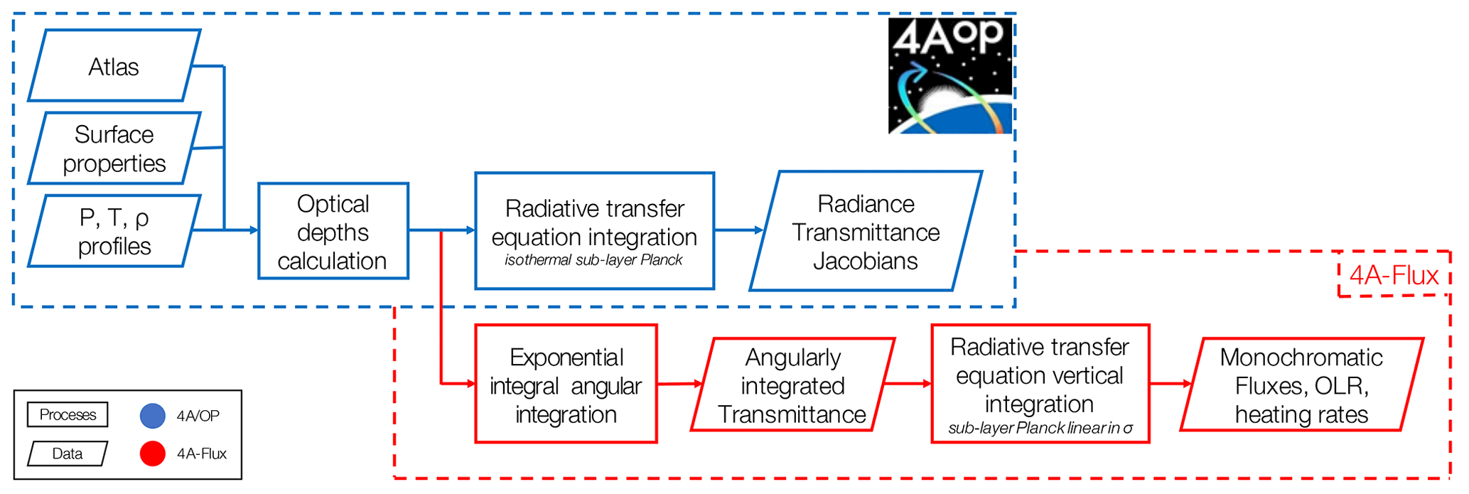
Figure 14A/OP and 4A-Flux flowchart. P, T, and ρ are the pressure grid, the temperature profile, and the profiles of gas concentrations, respectively.
Figure 1 presents the flowchart of 4A/OP with its new module 4A-Flux. The 4A/OP model provides a suitable basis for the computation of the radiative fluxes as it computes the vertical distribution of total optical depths at the spectral resolution of absorption lines. The inputs of 4A/OP are the atlases, a user-defined description of the pressure grid, the vertical distribution of temperature and gas concentrations, and surface properties such as surface temperature and spectral emittance. In this work, the spectroscopic database used in the calculation of the atlases is GEISA-2015 (Jacquinet-Husson et al., 2016); the continuum used is the MT_CKD 3.2 continuum (Mlawer et al., 2012), and the CO2 line mixing is the Lamouroux et al. (2015). Note that Lamouroux et al. (2015) is based on the parameters of HITRAN2012. Ongoing efforts will soon lead to a CO2 line mixing that will be based on the 2020 edition of the GEISA database (Delahaye et al., 2021). The pressure grid, the vertical distribution of temperature and gas concentrations, and surface properties such as surface temperature and spectral emittance can be specified by the user. Based on this description of the atmosphere and optical properties of gases, 4A-Flux computes the upwelling and downwelling monochromatic radiative flux profiles, also referred to as hemispherical monochromatic flux profiles [unit: ]. This computation is based on an exponential integral evaluation to perform the angular integration and a vertical integration. In the distributed version of 4A/OP, the vertical integration of the radiative transfer equation is performed under the assumption of isothermal layers (emission at the mean layer temperature), whereas in 4A-Flux, to better represent the real emission of each layer, we have implemented a sub-layer Planck function that varies linearly with the optical depth. 4A-Flux also offers the option of computing the monochromatic outgoing longwave radiation (OLR) instead of the full vertical description of fluxes, allowing a gain of computational time whenever the user does not require the complete vertical description of fluxes. The output spectral resolution is set by default to 1 cm−1 but can be specified by the user at any other value. The net monochromatic flux profile and the monochromatic heating rate vertical profile are then derived from the hemispheric profiles. The following section defines the radiative quantities and all the assumptions that have been made. We first focus on the definition of the downwelling flux, and then we treat the upwelling flux; finally, all the derived quantities that are computed by 4A-Flux are defined.
2.2 The computation of fluxes and heating rate profiles
The monochromatic3 hemispheric fluxes [unit: ], denoted F↓(σ) for the downwelling flux and F↑(σ) for the upwelling flux, are represented here by functions of σ, the monochromatic optical depth [unit: dimensionless] for all accounted gases in the model, as seen from the top of the atmosphere (TOA), where σ is null, to the bottom of the atmosphere (BOA) where it reaches its maximum value σBOA. Here, σ serves as a vertical coordinate as it increases monotonically with the pressure. The hemispheric fluxes are defined as the integrals of the monochromatic hemispheric radiances and [unit: ] over the respective hemispheres (Stamnes et al., 2017; Liou, 2002). These are defined as functions of the vertical coordinate σ, the azimuthal angle ϕ, and the direction μ=|cos (θ)|, which is the absolute value of the cosine of the zenith angle θ, where for the downwelling flux and for the upwelling flux:
As our computations are performed on the longwave spectrum and for clear-sky conditions, we assume the atmosphere to be non-scattering, and we neglect the radiance of the sun. We also assume an isotropic thermal emission of gases. Under such assumptions, the radiance is independent of the azimuthal angle, and thus we replace by . By integration with respect to ϕ we obtain
2.2.1 Downwelling flux
We focus on the downwelling flux in this section. Under the hypotheses of local thermodynamic equilibrium and local stratification of the atmosphere (plane-parallel geometry), the radiative transfer equation can be solved for the radiance. As we focus on the longwave only, the radiative contribution of deep space (less than 3 K) to the downwelling flux is negligible compared to the atmospheric contribution. Thus, the only remaining term in the solution of the radiative transfer equation is the atmospheric component, commonly referred to as the Schwarzschild equation:
Thus, by inserting Eq. (3) into Eq. (2), we obtain
where B[T(σ′)] is the Planck function [unit: ] evaluated at wavenumber ν (omitted in the notation) and at temperature T(σ′) [unit: K]. By switching the integration order, we can rewrite the downwelling flux as
Here, we have used the exponential integral of order n defined for n>0 and x≥0 as
In addition to the notation simplifications they allow, these series of functions present convenient mathematical properties. Their values at the origin are
They also follow simple recurrence relations:
This formulation is commonly used to compute fluxes (Stamnes et al., 2017; Feigelson et al., 1991; Ridgway et al., 1991). The exponential integral functions can be evaluated numerically even though the computational time is significant in the context of a line-by-line flux calculation. To overcome this limitation, 4A-Flux uses a tabulation of the En functions that is pre-calculated using the GNU Scientific Library (https://www.gnu.org/software/gsl/, last access: 12 June 2022).
In order to compute the downwelling flux for the discretized model of the atmosphere used in the 4A/OP model, we decompose the vertical integral into sums over every layer of the atmosphere. The atmospheric column is decomposed into N+1 levels using subscripts denoted k ranging from 0 to N or N layers using subscripts denoted with k ranging from 1 to N. We denote the value of the optical depth between the TOA and any level k as σk. At the TOA σ0=0, and at the surface σN=σBOA. At the TOA, the downwelling flux is supposed null, , and for every level k>0, we have
To compute the atmospheric contributions of each layer to the fluxes (the integrand of Eq. 9) an assumption has to be made about the variation of the Planck function at sub-layer scale. The simplest assumption considers the Planck function to be uniform at the sub-layer scale (isothermal layer) and evaluated at the average temperature of the layer , where . This assumption is a rather coarse approximation of the effective emission of the layer, especially when the optical depth is important. In such a case, the effective temperature is closer to the lower (upper) boundary of the layer for the downwelling (upwelling flux). A better assumption should take into account that the effective emission temperature is related to the optical depth of the layer. Thus, in our approach we have considered a sub-layer variation of the Planck function as linear in optical depth (also referred to as B(σ) linear). According to Ridgway et al. (1991), this approach dates back to Schuster (1905). Under such an assumption, the sub-layer variation of the Planck function in the layer and for the downwelling flux at level i is approximated by
The assumption of an isothermal layer would lead to a systematic cold (warm) bias in estimated downwelling (upwelling) fluxes (Ridgway et al., 1991), whereas the B(σ) linear assumption substantially reduces this bias (the remaining bias is discussed by Wiscombe, 1976). To better understand this approximation, one can verify that Eq. (10) is equivalent to the isothermal layer assumption when the layer optical depth tends to zero and is equivalent to the Planck function taken at the lower (upper) layer boundary temperature for the downwelling (upwelling) flux when the layer optical depth tends to infinity. For a more detailed explanation the reader can refer to Clough et al. (1992). Thanks to the B(σ) linear approximation, the downwelling flux can be integrated. To simplify the notations, we introduce the optical depth between two levels i and j as (for ). The downwelling flux, for every level k>0, can finally be expressed as
The first sum in Eq. (11) can be viewed as the cumulative downwelling flux emitted at the temperature of the lower boundary of every layer, whereas the second sum brings the correction needed to account for the fact that the equivalent temperature of emission is somewhere between lower boundary temperature T(σi) and the average layer temperature depending on the value of the optical depth of the layer .
2.2.2 Upwelling flux
Now that the downwelling flux has been treated, we will focus on the monochromatic upwelling flux. Unlike for the downwelling flux of Eq. (4) where the downwelling radiance only accounts for the atmospheric component, the upwelling radiance must also account for the surface emission and the reflection of the downwelling flux on the surface. Thus, the upwelling flux is written as
The first term of this equation is the contribution of the atmospheric emission to the upwelling flux, which is analogous to the downwelling flux of Eq. (4), replacing the boundaries of the integral and the argument of the exponential function. The second term is the contribution of the surface emission at temperature Ts considering a surface spectral diffuse emittance ϵ [unit: dimensionless] at wavenumber ν (omitted in the notation). The third term represents the contribution of the downwelling flux that is reflected on the surface and consequently contributes to the upwelling flux. The presence of a reflected contribution to the upwelling flux is the consequence of the fact that the surface does not behave exactly as a black body. The flux emerging from the surface must take the spectral emittance of the surface into account. Under the assumption of specular reflection we have .
For the atmospheric component at level k, denoted , we follow the same rationale as we previously have for the downwelling flux. However, we have to rewrite Eq. (10), replacing B[T(σi)] by B[T(σi−1)] and by , to account for the change in direction of propagation. And, we also have to integrate the radiance from the BOA to level σk instead of integrating from the TOA to level σk. We have , and for every level k<N we finally obtain
The surface component at level k, denoted , can be rewritten using the E3 function as
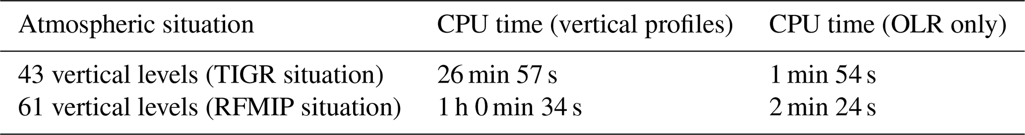
Table 1CPU time of the complete radiative transfer including calculation of radiative quantities for a single atmospheric situation.
For the reflected component at level k, denoted , the integration of the third term of Eq. (12) leads to
This equation can be understood by comparison to the equation for the downwelling flux (Eq. 11). The first difference is the (1−ϵ) factors before the sums that correspond to the fraction of downwelling radiation that is reflected by the surface. The second difference to Eq. (11) is that we sum all the layers from 1 to N because the reflected flux is a fraction of the downwelling flux that reaches the BOA. Finally, the third difference is the argument of the En functions. These arguments are now incremented by ΔN,k, which corresponds to the optical depth from the surface to the level k (upwelling propagation after the reflection).
2.2.3 Radiative quantities
In 4A-Flux, the total upwelling flux is finally obtained by adding the three contributions described above:
Once the monochromatic hemispherical fluxes are computed using Eqs. (11) and (16), 4A-Flux computes the net flux denoted F(σk) using the following convention:
The monochromatic OLR is simply defined as the net flux at the TOA F(σ0).
The monochromatic vertical heating rate, denoted H (omitted spectral dependence), is defined as the divergence of the net flux and is conventionally expressed in units of Kelvin per day [unit: K d−1]. It is the radiatively induced time rate of change in temperature T within a layer of the atmosphere. In the plane-parallel geometry, it is defined as
where g is the acceleration due to gravity and cp is the specific heat of dry air at constant pressure. The heating rate is usually negative for the longwave, and thus the expression cooling rate is sometimes preferred to the expression heating rate that we are using here. This quantity represents the rate of change in temperature caused by radiative properties of the atmosphere. In 4A-Flux, the computation of the heating rate at every layer is performed from the net flux of adjacent levels k and k−1 by calculating the difference quotient:
We then convert the heating rate from SI units to the commonly used K d−1 unit.
The computation time of the total radiative transfer including the calculation of the hemispherical fluxes, the net flux, and the heating rate profile is indicated in Table 1. The longwave fluxes are computed at the spectral resolution of the 4A/OP model (5 × 10⁻⁴ cm−1) from 10 to 3250 cm−1. The computation in the “OLR-only” option is a lot faster than the complete vertical profile computation. Indeed, to calculate the OLR the only requirement is to add up the contributions of the emission of all layers i that are transmitted to the TOA level. Therefore, the computational time is approximately proportional to the number of levels N. On top of the previous computation of linear computational complexity, the complete vertical profile requires the addition of the contributions of the emission of every layer i transmitted to every level k above layer i (below) for the upwelling (downwelling) flux. Therefore, the computational time is proportional to , and the computational complexity is quadratic. The additional terms required for the complete vertical profile are not required for the OLR calculation. This can be deduced from Eqs. (11), (13), and (15) in which it can be seen that the factors not only depend on the emission layers, but also on the level at which the fluxes are computed.
Cheruy et al. (1995)Scott and Chedin (1981)Buehler et al. (2018)Dudhia (2017)Edwards and Slingo (1996)Walters et al. (2019)Clough et al. (2005)Table 2List of the six benchmark models that have contributed to RFMIP-IRF and that are compared in this study.
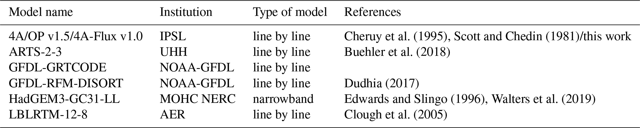
IPSL: Institut Pierre Simon Laplace; UHH: Universität Hamburg; NOAA-GFDL: National Oceanic and Atmospheric Administration, Geophysical Fluid Dynamics Laboratory; MOHC: Met Office Hadley Centre; NERC: Natural Environment Research Council; AER: Research and Climate Group, Atmospheric and Environmental Research.
The Radiative Forcing Model Intercomparison Project (RFMIP4; protocol paper: Pincus et al., 2016) is one of the 23 intercomparison projects supported by the World Climate Research Program (WRCP) in the context of the 6th phase of the Coupled Model Intercomparison Project (CMIP6, see Eyring et al., 2016). The objective of the experiment RFMIP-IRF (RFMIP Instantaneous Radiative Forcing from greenhouse gases) is to characterize the accuracy of the parameterization of the IRF used in climate models under clear-sky and aerosol-free conditions. This characterization is performed in comparison to line-by-line radiative transfer models that are recognized for their very high accuracy. Thanks to the new implementation of the 4A-Flux module, the 4A/OP radiative transfer model contributed to RFMIP-IRF by providing longwave downwelling and upwelling fluxes. Calculations of radiative forcing by greenhouse gases with the six benchmark models that are participating in RFMIP-IRF, 4A/OP included, are listed in Table 2. These models and the radiative forcing evaluation results are presented in Pincus et al. (2020).
RFMIP provides a sample of 100 atmospheric situations from reanalysis of present-day conditions containing profiles of pressure, temperature, greenhouse gas concentration, and surface properties. When averaged using the provided weights, the fluxes estimated from individual profiles can be used to estimate the time-averaged global mean fluxes with very small sampling errors (relative to disagreements between models). Along with the 100 present-day atmospheric situations, 17 perturbations around the present day are also provided, leading to a total sample size of 1800 atmospheric situations (perturbations are listed in Appendix A). All six benchmark models have provided longwave integrated upwelling and downwelling flux profiles for the whole set of atmospheric profiles.
Participating models have usually provided several sets of spectrally integrated longwave flux profiles for slightly different sets of greenhouse gases, called forcing variants as described in Meinshausen et al. (2017). For the first forcing variant (denoted f1), models are free to use any subset of the 43 greenhouse gases specified in Meinshausen et al. (2017). For forcing variant f1, 4A/OP takes into account 16 gases out of the 43 gases included into the RFMIP database5. Both the second and third forcing variant (respectively denoted f2 and f3) use CO2, CH4, and N2O. In addition to those three gases, forcing variant f2 also uses CFC-12 concentration and a modified concentration of CFC-11 to account for all omitted gases, whereas forcing variant f3 uses modified concentrations of CFC-11 and HFC-134a to represent all omitted gases.
Some participating models have also provided several sets of results based on slightly different model configurations, called physics variants. As described in Pincus et al. (2020), the model ARTS 2.3 only includes CO2 line mixing for physics variant p2 and not for physics variant p1. The model HadGEM3-GC3.1 physics variant p1 uses a lower spectral resolution than physics variant p2 that corresponds to the high-resolution configuration. The physics variant p3 is the high-resolution configuration with MT_CKD 3.2 treatment of the water vapor continuum instead of the CAVIAR continuum.
Using the RFMIP database, we have evaluated the downwelling and upwelling fluxes computed with the 4A-Flux module of the 4A/OP model against calculations of other participating radiative transfer models. To perform this comparison, we have averaged downwelling and upwelling fluxes for the 1800 atmospheric situations using the provided weights to average the 100 atmospheric situations and uniformly averaging the 18 perturbations. For any given pair of model and physics variant, we have also averaged the downwelling and upwelling fluxes for every provided forcing variant. Forcing variants are averaged for clarity purposes as for every model, variability between forcing variants is smaller than the variability between models and physics variants (not shown here). For HadGEM3-GC3.1, we have not retained the physics variant p1 for the comparison as it uses a lower spectral resolution and thus would not usefully serve as a reference. Figure 2 shows the distance from the mean downwelling and upwelling flux profiles of each model i to the mean of all profiles for the eight retained model–physics variant pairs. This distance is computed as
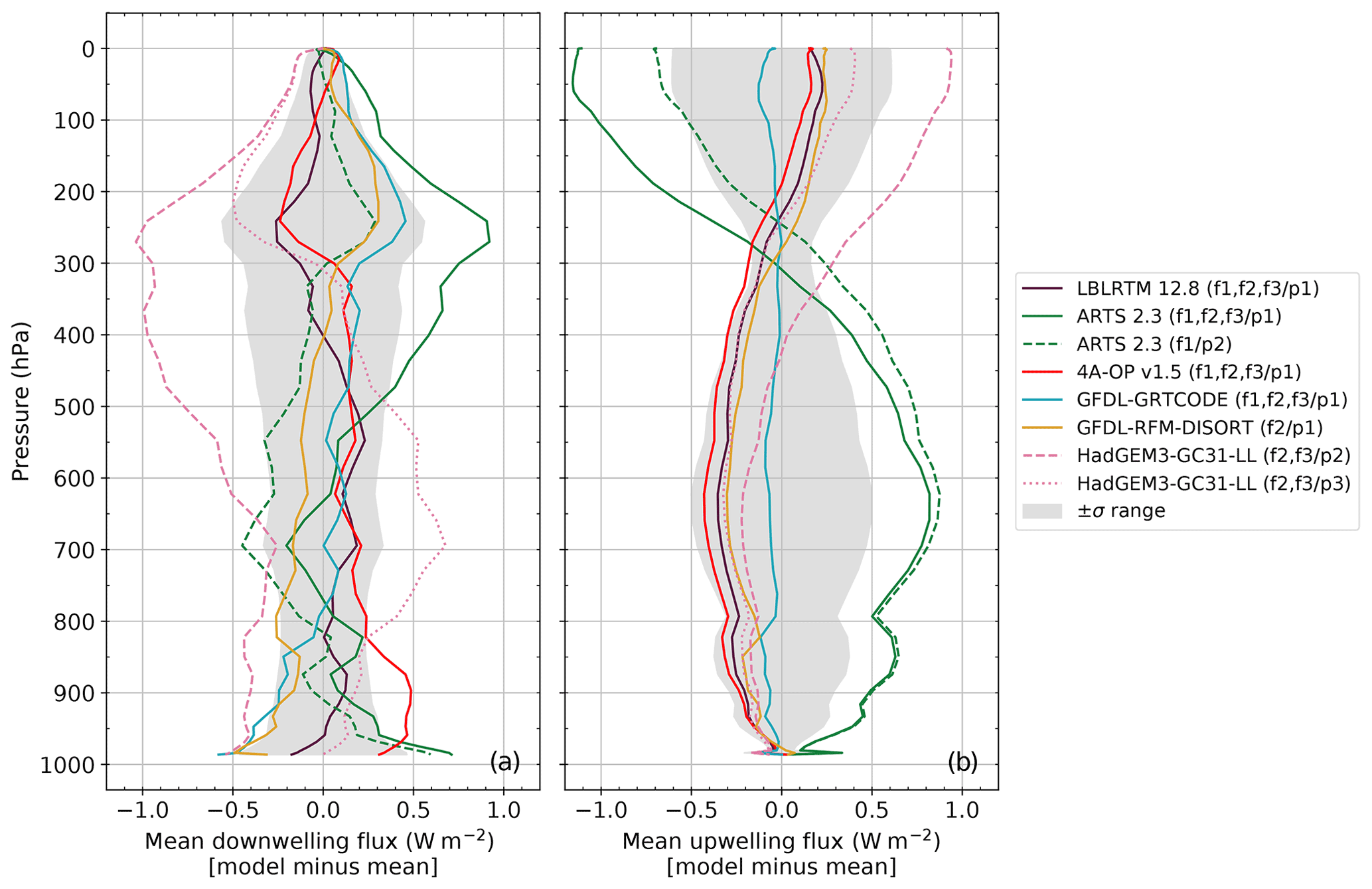
Figure 2Comparison of net flux profiles between line-by-line models participating in RFMIP-IRF. Panels (a) and (b) respectively show the distance to the mean of the mean downwelling and upwelling flux profiles for every pair of model and physics variant. The averaging is first performed on the 100 atmospheric profiles using provided weights and then on the 18 perturbations (uniformly weighted). Finally, for every pair of model and physics variant, all available forcing variants are averaged. The ± 1 standard deviation range (±σ) is represented by the gray shaded area.
The ± 1 standard deviation range between models is also displayed in Fig. 2 (gray shaded area). We first notice the strong agreement between all compared models. The standard deviation between models is smaller than 0.61 W m−2 for the downwelling flux and 0.75 W m−2 for the upwelling flux. 4A/OP model outputs are included in the ± 1 standard deviation range at almost every level with the exceptions of the 993–976 hPa pressure range for the downwelling flux and of the 300–401 hPa pressure range for the upwelling flux; they nonetheless stay close to the ± 1 standard deviation range. The extremum difference for the 4A/OP model ranges from −0.24 to 0.49 W m−2 for the downwelling flux profile and from −0.43 to 0.20 W m−2 for the upwelling flux profile.
Table 3Means and standard deviations of OLR differences (model minus 4A/OP) in W m−2.
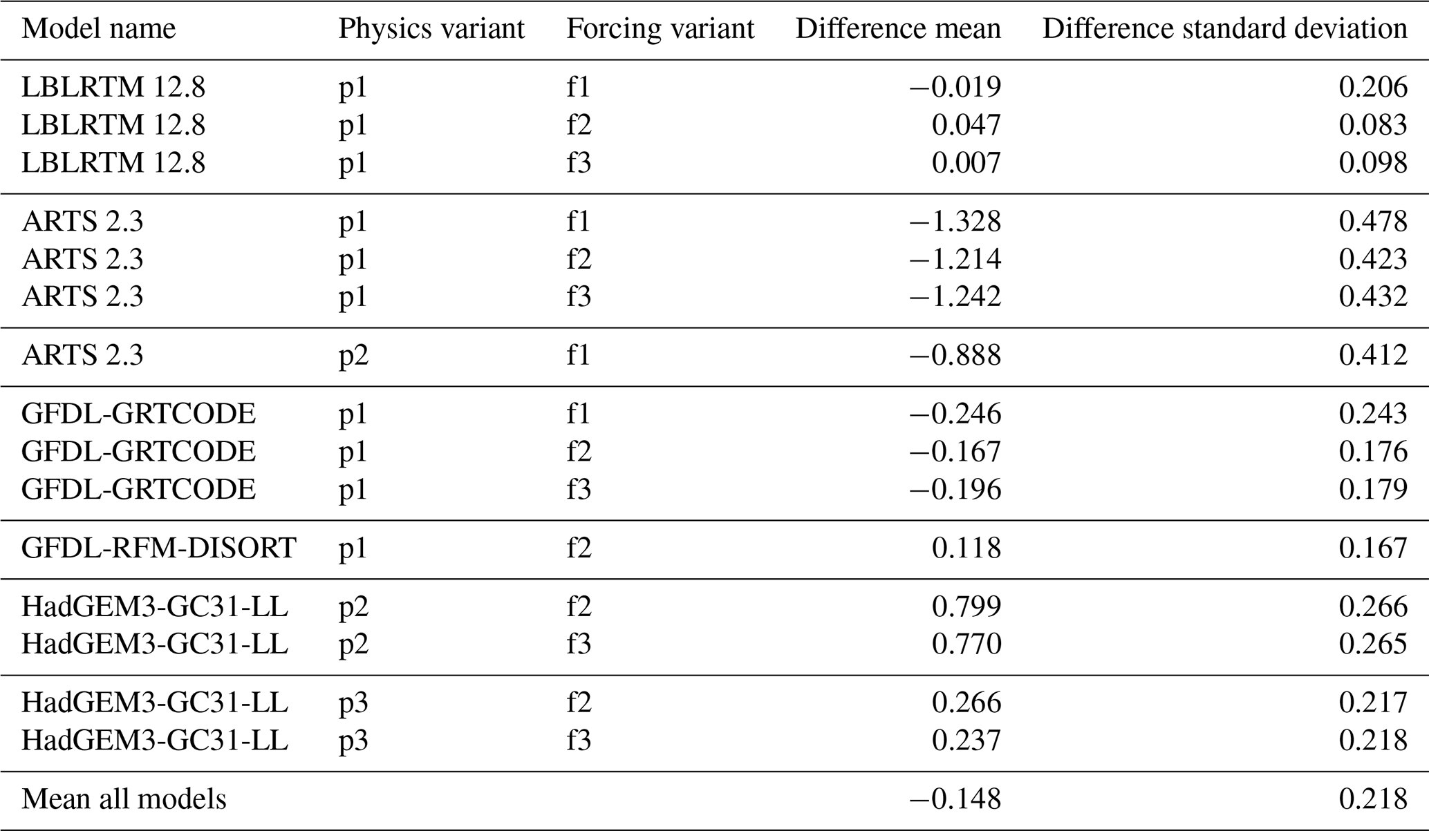
The OLR estimations are compared using the same averaging methodology. However, we have not averaged forcing variants to give more detailed results. The statistics for all models are calculated by first averaging forcing variants for every model–physics variant pair, and then we average these pairs together. Table 3 presents these statistics (model minus 4A/OP). The mean difference between 4A/OP and other models is −0.148 W m−2 and the mean standard deviation is 0.218 W m−2. This shows very good agreement between 4A/OP and other models. Note that 4A/OP simulates OLR values that are very close to the LBLRTM simulations, especially for forcing index f2 and f3 for which the exact same gas list has been simulated. In the forcing index f3, the mean difference between 4A/OP and LBLRTM is 0.007 W m−2 with a difference standard deviation of no more than 0.098 W m−2. The difference to all models is always smaller than 1 W m−2 except for ARTS physics index p1 that does not include CO2 line mixing. The greater observed difference in standard deviation noticeable for forcing variant f1 compared to f2 and f3 variants is due to the gases that are not yet implemented in 4A/OP and thus not simulated in f1, whereas all gases of f2 and f3 are identical between models. This is further explained in Appendix A where experiments, forcing, and physics variants are compared without any averaging.
The results of this comparison show very good agreement of 4A/OP with the five other participating models. The 4A/OP simulation yields results to LBLRTM, especially for the longwave upwelling flux and the OLR. This good very close agreement, while the two models differ completely in both numerical methods and the spectroscopic databases used (GEISA for 4A/OP, HITRAN for LBLRTM), is an important factor in the confidence that we can have in their results. Furthermore, these deviations between models are well below the sensitivities to typical perturbations of surface and atmospheric parameters that we will describe next.
In this section, we present a first application of the 4A-Flux module newly implemented in the radiative transfer code 4A/OP. Following Clough and Iacono (1995), we perform a sensitivity study of the OLR and the vertical heating rate to various atmospheric and surface parameters. This sensitivity is based on the Thermodynamic Initial Guess Retrieval (TIGR) atmospheric database that is developed at the Laboratoire de Météorologie Dynamique. We will first present the TIGR database and then describe the sensitivity study that we have performed on the OLR and on the longwave vertical heating rate.
4.1 TIGR atmospheric database
The Thermodynamic Initial Guess Retrieval (TIGR) atmospheric database is a climatological library containing 2311 atmospheric situations that have been carefully selected by statistical methods from radiosonde reports (Chédin et al., 1985; Achard, 1991; Chevallier et al., 1998). The atmospheric samples are described by their vertical profiles of temperature, water vapor, and ozone concentration on a pressure grid of 43 levels. The pressure levels range from the surface at 1013 up to 0.0026 hPa and the density of points along the vertical increases, while pressure decreases to correctly account for the upper atmospheric layers. The 2311 atmospheres are classified into five air mass types. The Tropical class contains situations in the tropics, the Midlat 1 class contains midlatitude situations, the Midlat 2 class contains cold midlatitude and summer polar situations, the Polar 1 class contains Northern Hemisphere very cold polar situations, and the Polar 2 class contains winter polar situations for both hemispheres. This classification has been performed by a hierarchical ascending classification depending on their virtual temperature profiles (Achard, 1991; Chédin et al., 1994).
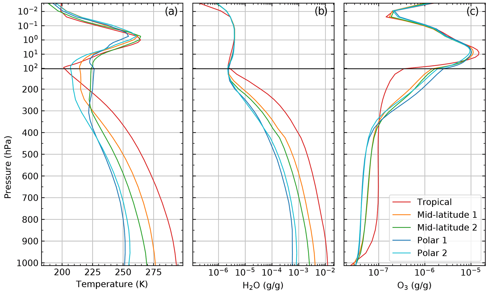
Figure 3Average atmospheric profiles of temperature (a), water vapor concentration (b), and ozone concentration (c) of the mean atmosphere of each of the five classes of TIGR. The temperature profile is presented on a linear scale, whereas the concentration profiles are presented on a logarithmic scale in units of grams of gas per gram of dry air. The upper panels present the profiles on a logarithmic pressure scale, and the lower panels present them on a linear pressure scale.
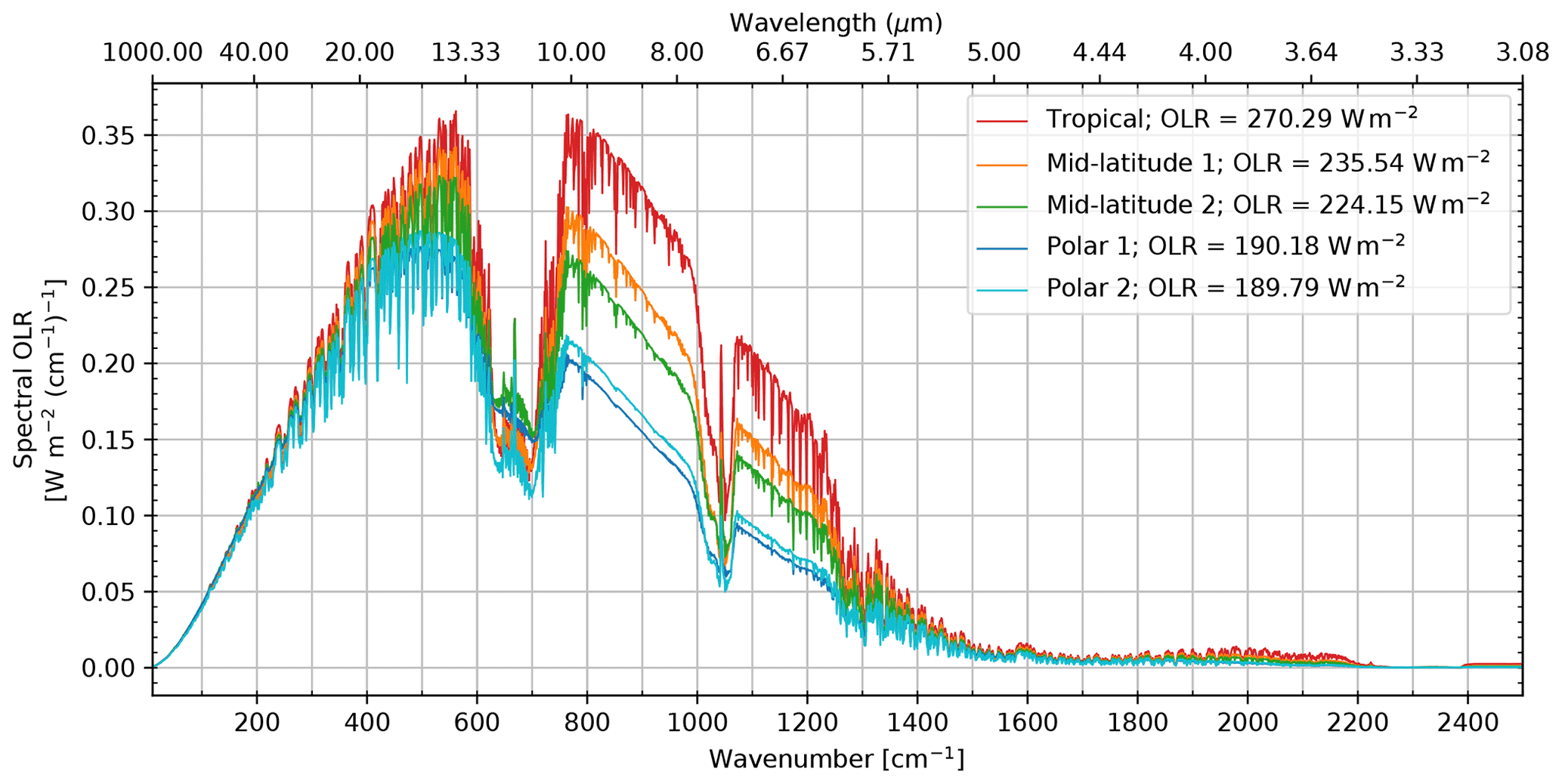
Figure 4Spectral OLR at a resolution of 1 cm−1 computed for the mean atmosphere of each of the five classes of TIGR. Spectrally integrated OLR values in the 10–2500 cm−1 range are displayed in the legend.
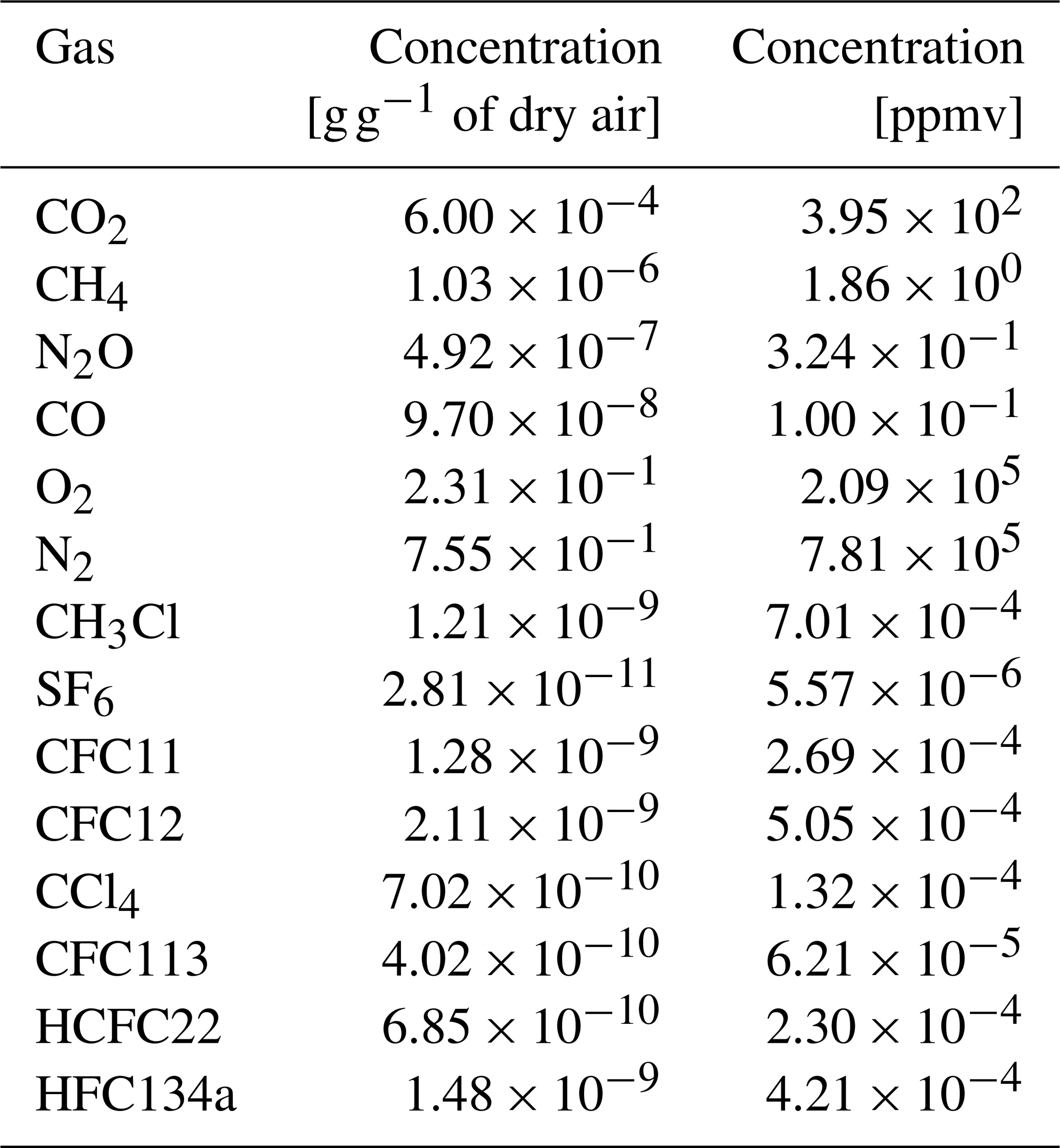
Figure 3 represents the mean profiles of temperature, water vapor, and ozone concentration computed for each of the five classes of the TIGR database. OLR value calculated by 4A-Flux using these five averaged atmospheres are represented in Fig. 4. Except for temperature, water vapor, and ozone, other simulated variables are identical for all five atmospheres. Table 4 presents the concentration of well-mixed greenhouse gases (WMGHGs) considered as a reference for our simulations. For all the simulations we perform here, the surface spectral diffuse emittance is set at a constant value of 0.98 on the entire longwave spectrum. To be more concise, the averaged atmospheres of the five classes will be called by the name of their class (e.g., Tropical atmosphere or Tropical situation instead of mean atmosphere of the Tropical class).
Table 4Concentration of WMGHGs and minor gases used for the simulation. The concentrations of all these gases are assumed to be vertically constant.
The Tropical temperature at the surface and in the troposphere is significantly higher than all other classes, especially both Polar situations that exhibit lower temperatures. Higher temperatures lead to a higher OLR, which is especially noticeable in the atmospheric IR window. This difference is lower where the absorption is important such as on the carbon dioxide ν2 absorption band. At the tropopause, the temperature profile of the Tropical situation is the lowest. Above the tropopause, the temperature profiles are closer together.
Mainly present in the troposphere, water vapor is 15 times more concentrated at the surface of the Tropical atmosphere than at the surface of both Polar atmospheres. The Tropical atmosphere has the highest water vapor content compared to all other classes, especially compared to the dry atmospheres of the Polar classes. Consequently, we observe less of an impact of water vapor absorption on the OLR spectra of the drier atmospheres.
In all atmospheres, the ozone concentration is high in the stratosphere and in the mesosphere and relatively low in the troposphere. However, it is less spread and peaks higher in the Tropical class compared to other classes. Thus, the OLR of the mean Tropical atmosphere has more of an impact on the ozone absorption band than all other classes.
As they represent very different and opposite situations, we will only focus next on two specific classes: the hot and humid Tropical class and the cold and dry Polar 2 class. We will now present the results of a sensitivity study of the OLR and longwave heating rate profile to several perturbations of surface and atmospheric parameters using TIGR Tropical and Polar 2 atmospheric situations as input of the 4A/OP model.
4.2 OLR sensitivity
Here, we seek to quantify the effects of perturbations applied to atmospheric and surface parameters on the OLR spectrum and on the spectrally integrated OLR. To perform this analysis, we have calculated the OLR differences between a reference atmosphere and a modified atmosphere affected by a series of perturbations. The reference atmospheres used here are computed with the TIGR mean Tropical and mean Polar 2 atmospheric situations that are presented in Sect. 4.1. We first present the reference OLR spectra in both Tropical and Polar 2 situations, and then we present the effects of several thermodynamic and composition perturbations. We will describe the effects of an increase in surface temperature of 1 K above the reference and of a vertically uniform increase in the atmospheric temperature of 1 K. And, we will analyze the effects doubling the concentrations of the three main WMGHGs: carbon dioxide, methane, and nitrous oxide. Each perturbation is studied independently of one another and applied uniformly on the vertical profile. And then, we will examine the effects of a +1 % vertically uniform increase in water vapor concentration and ozone concentration.
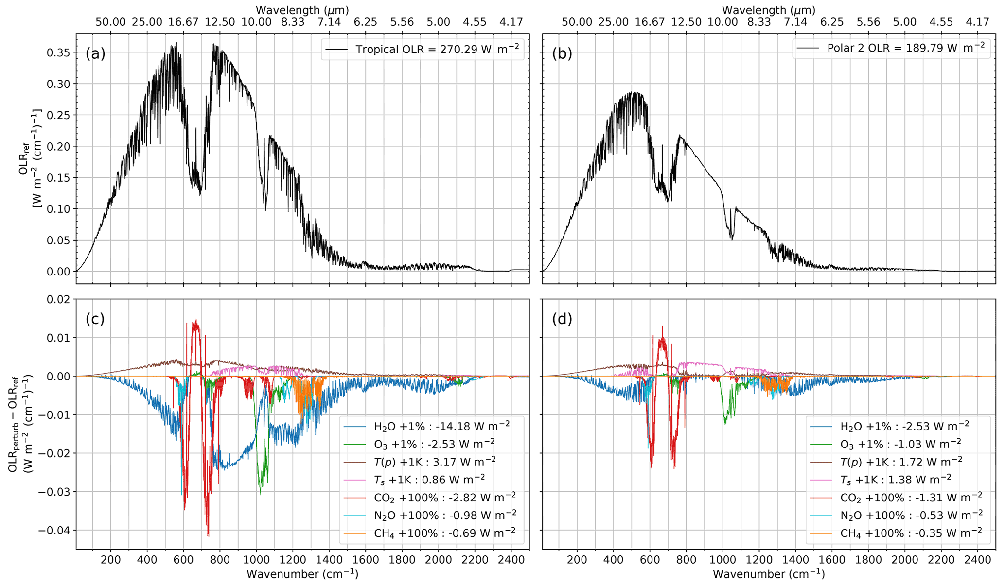
Figure 5Spectral OLR at a spectral resolution of 1 cm−1 computed for the TIGR mean Tropical atmosphere (a) and TIGR mean Polar 2 atmosphere (b). Corresponding OLR values spectrally integrated between 10 and 2500 cm−1 are provided in the legends. Spectral OLR sensitivity to temperature and composition change for the TIGR mean Tropical (c) and mean Polar 2 (d) atmospheres. Results are expressed as [OLRperturb.−OLRref.] as a function of the wavenumber. The spectrally integrated sensitivities are specified in the legends and in Table 5.
Table 5Spectrally integrated OLR sensitivity to the variations of thermodynamic and composition variables.
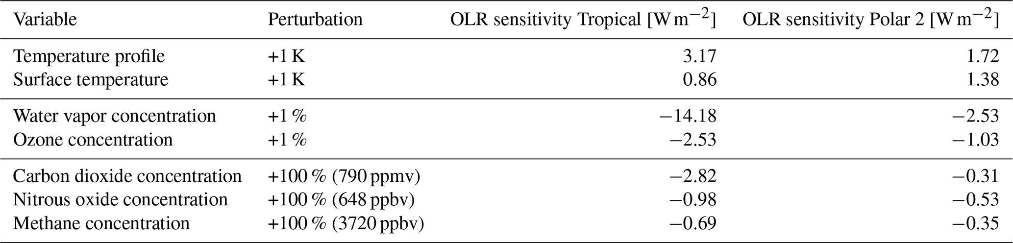
Figure 5 presents the OLR spectra at resolution 1 cm−1 simulated by the 4A-Flux module in the Tropical situation in Fig. 5a and in the Polar 2 situation in Fig. 5b. Figure 5 also shows the effects of the studied perturbations on OLR as a function of the wavenumber in the Tropical situation in Fig. 5c and in the Polar 2 situation in Fig. 5d. Table 5 summarizes the spectrally integrated OLR variation caused by these perturbations.
The Tropical OLR spectrum and longwave integrated OLR (panel a) are greater than the Polar 2 OLR spectrum (panel b). This is mainly due to the substantially higher surface and atmospheric temperatures of the Tropical situation compared to the Polar 2 situation (almost 40 K difference between the surface temperatures). The well-known signatures of the main longwave active gases are also clearly visible in Fig. 5: carbon dioxide (580–750, 2200–2400 cm−1), ozone (980–1080 cm−1), water vapor (especially the far infrared and large band around 1600 cm−1), methane, and nitrous oxide (1250–1350 cm−1).
According to Eq. (14), the increase in the surface temperature is expected to lead to an increase in the surface Planck emission for all wavenumbers at the BOA. At the TOA, the OLR is expected to increase only in the atmospheric IR window. This is well verified here in panels (c) and (d) (pink curve). With the Tropical atmosphere being optically thicker (higher humidity), the OLR sensitivity is spectrally confined to the infrared atmospheric window compared to the Polar 2 atmosphere. Because the atmospheric window spectral range is relatively free from absorbers other than water vapor, a lower concentration of water vapor leads to a higher OLR sensitivity to the surface temperature in this spectral range.
The vertically uniform increase in the atmospheric temperature profile is expected to lead to an increase in the Planck emission of every layer of the atmosphere (Eq. 13), leading to an increase in the OLR on bands where there is gas absorption (assuming the absorption lines of the gases are marginally impacted by the temperature perturbation). This is also verified in Fig. 5. In the Tropical case, the increase extends to the whole longwave spectrum. However, for the dry Polar 2 atmosphere, there is very low absorption and emission on the infrared window.
The increase in the WMGHG concentration leads to a decrease in the surface contribution to the OLR (Eq. 14) as the total surface-to-space optical depth increases. For the contribution of the atmospheric layers to the OLR, however (Eq. 13), there is competition between the increase in the thermal emission of atmospheric layers (increasing the OLR) and the increase in absorption by gases (decreasing the OLR). The ν2 absorption band of CO2 shows a remarkable pattern. The increase in CO2 causes an OLR decrease in the band wings, where the absorption dominates; however, it causes an OLR increase in the band center, where the emission dominates. Integrated over the entire longwave, the absorption dominates, causing an OLR decrease in the longwave. Jeevanjee et al. (2021) clearly explain that in the absence of H2O, the CO2 forcing can be considered a swap of surface emission in band wings for the stratospheric emission in the band center and that, in the presence of H2O, the surface emission in band wings is being replaced by the emission of a colder atmosphere. In Fig. 5, in the tropical atmosphere (high RH) we observe on the CO2 band wings a high sensitivity shared between H2O and CO2, whereas in the Polar 2 atmosphere (low RH) the high sensitivity is shared between the surface temperature and CO2. The sensitivity of N2O (550–640, 1140–1320 cm−1) is dominated by the absorption, and we do not observe any local increase in OLR. The CH4 sensitivity (1200–1370 cm−1) is also dominated by the absorption.
Unlike for the WMGHGs, water vapor absorbs on the entire longwave region. The sensitivity to water vapor concentration is especially important in the Tropical situation and less important in the drier Polar 2 situation. In the Tropical case, the OLR decreases almost everywhere on the longwave spectrum, except where the ν2 carbon dioxide band dominates the absorption. In the Polar 2 case, the sensitivity to water vapor almost completely disappears in the atmospheric window. A reduction in water vapor sensitivity is also notable on spectral bands where other gases absorb and compete with water vapor absorption (O3 at 1000–1080 cm−1 as well as both CH4 and N2O at 1250–1350 cm−1). With water vapor being more concentrated in the lower troposphere, the WMGHGs play a relatively greater part at the TOA.
An increase in ozone concentration leads to an OLR reduction (600–800, 980–1080 cm−1). With ozone being more concentrated in the stratosphere around 100 hPa, an increase in its concentration leads to a decrease in the surface and the tropospheric and lower stratospheric contributions to the OLR. The increase in the emission to space is also present but remains small as it can be seen in the 600–700 cm−1 range wherein there is a local increase in the spectral OLR.
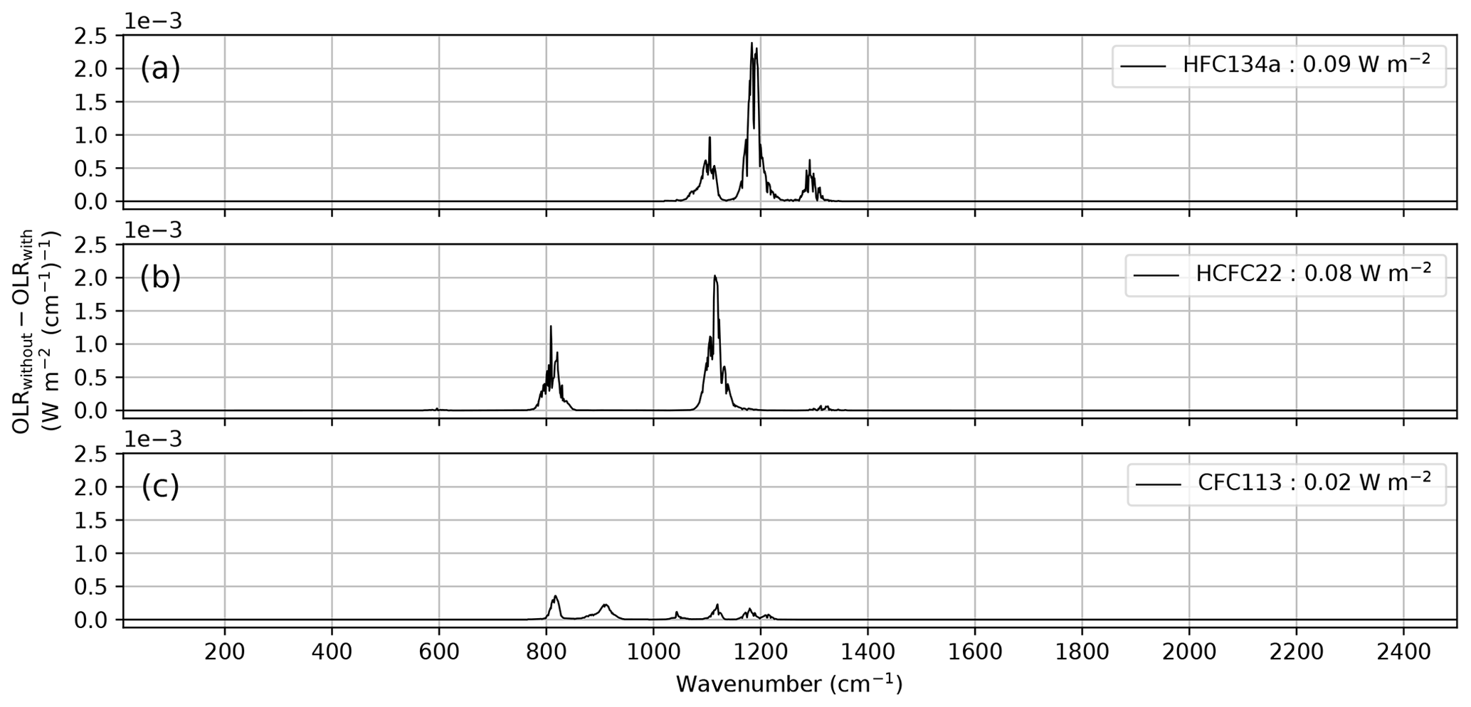
Figure 6Spectral OLR variation due to a complete removal of atmospheric HFC134a (a), HCFC22 (b), and CFC113 (c) calculated from the TIGR mean Tropical atmosphere. The total longwave OLR variations are reported in the legends. Note that the y axis ranges from 0 to 2.5 × 10⁻³ .
Figure 6 shows the OLR sensitivity to three anthropogenic trace gases: HFC134a, HCFC22, and CFC113. Even if their individual contributions to the total OLR are small, these three gases together represent 0.19 W m−2 for the tropical atmosphere, which is approximately the standard deviation between 4A/OP and other RFMIP benchmark models. However, as demonstrated and discussed by Pincus et al. (2020), the standard deviation between the six RFMIP benchmark models in terms of radiative forcing is less than 0.025 W m−2 – way below the standard deviation obtained from fluxes because of the cancelations when computing the radiative forcing as a difference of hemispheric fluxes (Pincus et al., 2020; Mlynczak et al., 2016). Accounting for more minor gases in line-by-line radiative transfer models could also improve our understanding of model intercomparison discrepancies.
These applications show that the 4A-Flux module of 4A/OP can be used to study OLR sensitivity to thermodynamic variables and composition of the atmosphere. Thanks to its very fine spectral resolution (down to 5 × 10⁻⁴ cm−1), 4A/OP can help evaluate the subtle impacts of minor longwave active gases such as HFC134a, HCFC22, and CFC113.
4.3 Vertical heating rate sensitivity
In this section, we focus on the sensitivity of the vertical heating rate profile caused by a vertically uniform increase of 1 % in the water vapor concentration and by a doubling in carbon dioxide concentration using the TIGR mean Tropical atmospheric situation and the TIGR Polar 2 atmospheric situation as reference atmospheres. First, we describe the longwave heating rate vertical and spectral distribution for the two reference atmospheric situations, and then we analyze the sensitivities that are calculated as the difference between the perturbed atmospheric state and the reference state: Hperturb.(p)−Href.(p).
Figure 7 presents the vertical heating rate as computed by 4A-Flux for the Tropical (Fig. 7a1 to c1) and Polar 2 (Fig. 7d1 to f1) atmospheric situations. Figure 7a1 and d1 show the vertical heating rate spectrum as a function of the wavenumber (horizontal axis) and the pressure level (vertical axis). Figure 7b1 and e1 show the heating rate profile spectrally integrated between 10 and 2500 cm−1. In Fig. 7c1 and f1, the range of the x axis has been modified to focus on the tropospheric variations. In all panels, the vertical representation has been divided into two separate pressure scales. The lower sub-panels, wherein the pressure scale is linear, highlight the tropospheric heating rate, and the upper sub-panels, wherein the pressure scale is logarithmic, give better insight into the heating rate above the tropopause. The color scale has been chosen to emphasize the main radiative signature of the different gases at multiple scales. Cool colors represent a net cooling, while warm colors represent a net heating, except magenta, which represents extreme cooling values.
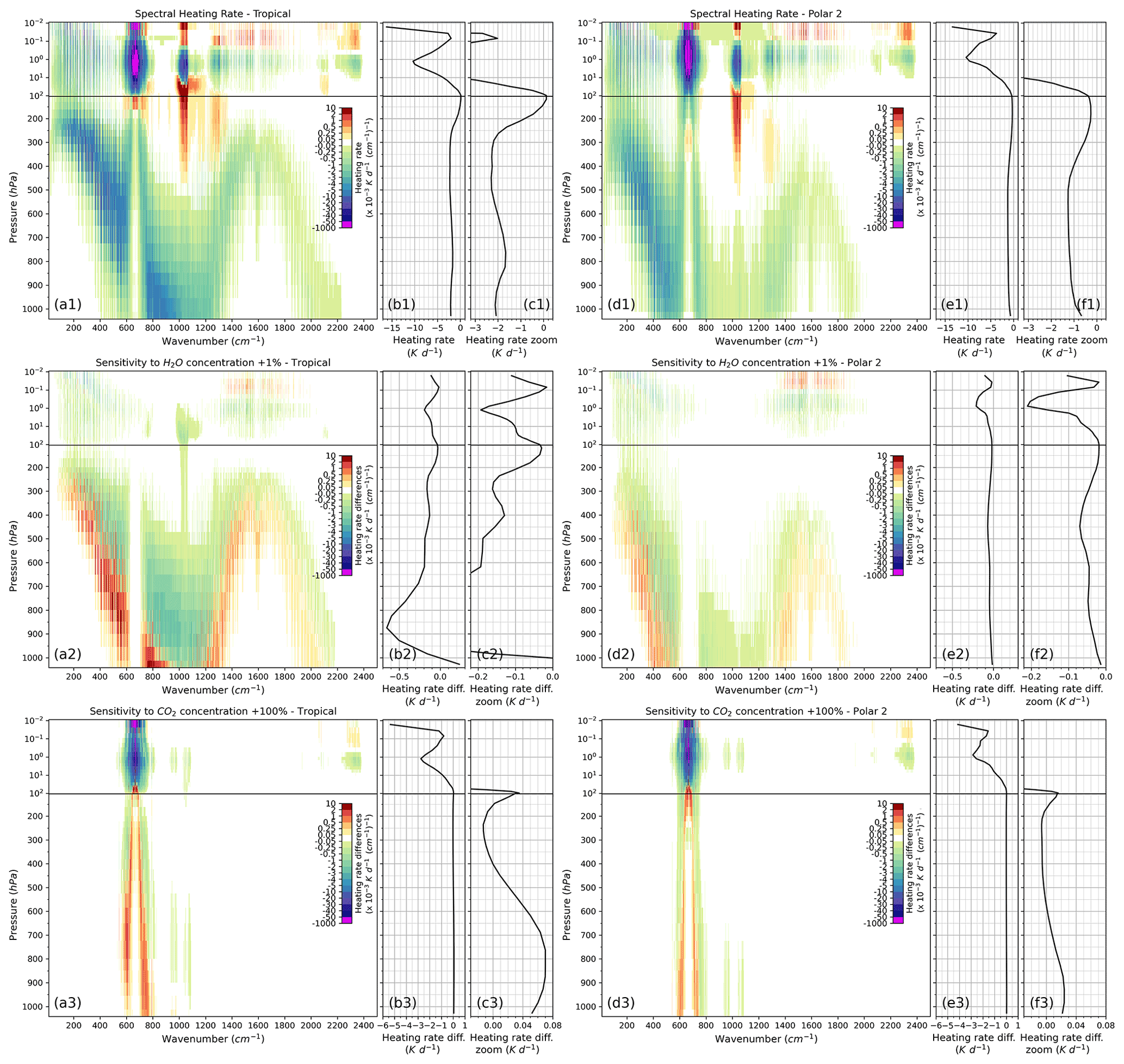
Figure 7Top row (a1–f1): vertical heating rate computed by 4A-Flux using TIGR mean Tropical (Polar 2) atmospheric situation in the left (right) panels. Panels (a1) and (d1) present the spectral heating rate profile as a function of the wavenumber and the pressure level. The heating rate profile integrated on the 10–2500 cm−1 spectral range is represented in panels (b1) and (e1), and a focus on the tropospheric variations is displayed in panels (c1) and (f1). Middle row (a2–f2): vertical heating rate sensitivity to a 1 % increase in H2O concentration. Panels (a2) and (d2) present the spectral heating rate sensitivity profiles [Hperturb.(p)−Href.(p)] as a function of the wavenumber (horizontal axis) and the pressure level (vertical axis). The heating rate sensitivity profile integrated on the 10–2500 cm−1 spectral range is represented in panels (b2) and (e2), and a focus on the stratospheric variations is displayed in panels (c2) and (f2). Bottom row (a3–f3): analog to the middle row for a doubling of CO2 concentration (instead of H2O). Panels (c3) and (f3) show a focus on the tropospheric variations.
Tropical and Polar 2 longwave integrated heating rate profiles show similarities (Fig. 7b1, c1, e1 and f1). The heating rate profiles are negative almost everywhere on the vertical and show a characteristic shape. In both cases, we notice that the profiles are almost constant in the troposphere before increasing around a certain pressure level, referred to as the kink, which is recognized to be associated with several atmospheric processes (Jeevanjee and Fueglistaler, 2020, and references therein). Above the kink, the heating rate increases and reaches its maximum value around 100 hPa where the heating rate is close to 0 K d−1. Above 100 hPa, the heating rate profile decreases again until 1 hPa, then increases until 0.1 hPa to finally decrease at the TOA. We also notice differences of heating rate profiles between the two atmospheric situations. First, the values of the heating rate until the kink are not the same (around −2 K d−1 in the Tropical case and −1 K d−1 in the Polar 2 case). Second, the kink occurs around 250 hPa in the Tropical atmosphere and around the 400 hPa in the Polar 2 atmosphere, which approximately corroborates the Tkink = 220 K specified in Jeevanjee and Fueglistaler (2020). Above the kink, we notice a greater slope in the Tropical atmosphere than in the Polar 2 atmosphere. As demonstrated in Jeevanjee and Fueglistaler (2020), the upper-tropospheric kink in the heating rate profile originates from the distribution of absorption coefficients in the water vapor rotational band. More precisely, in the H2O rotational band, the occurrence of more weakly absorbing wavenumbers is relatively constant, whereas the occurrence of more strongly absorbing wavenumbers sharply declines above a certain threshold corresponding to the kink observed in the heating rate profile. Being linked to the water vapor absorption, this also explains why the kink appears at different altitudes for the different scenarios.
The characteristic variations of the heating rate profile previously described can be further analyzed using the spectral and vertical distribution of absorption by longwave active gases. The representation in Fig. 7a1 and d1 give insight into these distributions. In both atmospheric situations, the spectra of heating rate profile display similarities. We observe the signatures of the greenhouse gases accounted for in the model. The water vapor effects dominate the Earth longwave cooling as it absorbs on a wide portion of the longwave spectrum. This is primarily due to the strong absorption of the pure rotational band peaking in the 100–200 cm−1 range but extending from the 10–1000 cm−1 range in the Tropical case. The water vapor effects are also caused by the relatively lower absorption by the rotational–vibrational band centered on 1600 cm−1 and by the continuum of absorption. The radiative cooling induced by the ν2 absorption band of carbon dioxide is dominant in the 580–750 cm−1 range. Due to the very high absorption of carbon dioxide in the band center, most of the radiative cooling occurs in the stratosphere. The cooling is very small under the tropopause temperature inversion, whereby a net heating occurs. Above this tropopause heating, an intense cooling occurs in the stratosphere and mesosphere until the TOA. On the band wings of the carbon dioxide ν2 absorption band, we observe a net cooling in the whole profile except at the tropopause in the Tropical case in which we observe a net heating. We observe the effects of the ozone absorption in its main absorption region: the 980–1080 cm−1 range. A strong heating occurs in the upper troposphere, tropopause, lower stratosphere, and high in the mesosphere, with an intense cooling in the upper stratosphere and stratopause. The same pattern, with a lower amplitude, appears in the 1250–1350 cm−1 range wherein methane and nitrous oxide absorb. The main differences of the heating rate profile spectrum between the Tropical and the Polar 2 atmospheres is the amplitude of cooling and the pressure range at which the cooling occurs. In the troposphere of the Tropical atmosphere, the cooling is more intense due to the association of a steeper temperature gradient and a higher water vapor concentration. We also notice that, due to the more vertically spread ozone concentration profile in the Polar 2 atmosphere compared to the Tropical atmosphere, the ozone cooling pressure range is wider.
The vertical heating rate sensitivity to a 1 % increase in water vapor concentration is presented in Fig. 7a2, b2, and c2 for the Tropical atmosphere and Fig. 7d2, e2, and f2 for the Polar 2 atmosphere. For the Tropical atmosphere, the spectrally integrated heating rate sensitivity profile shows a decrease in the heating rate at almost every level except for the first levels near the surface. The decrease is especially important in the 800–950 hPa range. Figure 7a2 informs us about the spectral distribution of this decrease. On both the pure rotational and rotational–vibrational transition bands, where water vapor absorption is important, we observe a heating rate increase at the level of minimum heating rate (maximum cooling rate) and a heating rate decrease of the same magnitude above the level of minimum heating rate. This behavior corresponds to an elevation of the altitude of the minimum heating rate. The decrease in heating rate in the ozone absorption band (980–1080 cm−1 range) in the upper troposphere and the stratosphere illustrates the competition between water vapor absorption and ozone absorption in this region of the longwave spectrum. Compared to the Tropical atmosphere, the impact of a 1 % increase in water vapor concentration on the relatively dry Polar 2 atmosphere is less important. As represented in Fig. 7e2 and f2, the vertical heating rate sensitivity is negative for all levels. In the troposphere, the decrease is limited to −0.07 K d−1. A noticeable decrease reaching −0.2 K d−1 is present in the upper atmosphere with the same amplitude as in the Tropical atmosphere. Visible in Fig. 7d2, this decrease is caused by the combination of contributions of the pure rotational and rotational–vibrational transition bands of water vapor adding up at levels between 0.1 and 1 hPa, while they compensate at higher levels. Here, we also notice the elevation of the altitude of the minimum heating rate in the troposphere.
Figure 7a3 to f3 present the vertical heating rate sensitivity to a doubling in carbon dioxide concentration. As can be seen in Fig. 7b3 and e3, the heating rate profile is slightly affected in the troposphere and highly affected in the stratosphere. In the Tropical case, we notice a small increase in the heating rate in the lower troposphere until 400 hPa. Above this level, the heating rate stays constant until the tropopause. In the Polar 2 atmosphere, we observe the same tropospheric effect with a diminished amplitude. The heating rate profile stops increasing at 400 hPa. In the stratosphere and above, Tropical and Polar 2 atmospheres show a sensitivity similar to the doubling of CO2 concentration. In this pressure range, we observe an important decrease in the heating rate. At the TOA, the cooling to space is more intense in the Tropical atmosphere than in the Polar atmosphere.
The analysis of the sensitivity spectrum shows that the main impact of doubling the CO2 concentration on the heating rate is located in the ν2 absorption band. In band wings, we notice an increase in the heating rate in the lower troposphere and a small decrease in the upper troposphere, followed by an important heating rate decrease in the stratosphere and above. In the band core, however, no change occurs under the tropopause. We notice a small increase in the lower stratosphere followed by a very high decrease in the upper stratosphere. In both atmospheres, we notice a small sensitivity in the stratosphere and mesosphere in the 2200–2400 cm−1 range.
Taking advantage of its pre-calculated optical depth lookup table, the fast and accurate radiative transfer model 4A/OP calculates the radiance spectra for a user-defined layered atmospheric model. In an effort to enhance the capabilities offered by 4A/OP, we have developed a module called 4A-Flux that computes the hemispheric radiative flux profiles, the net flux profile, and the heating rate profile in clear-sky conditions under the assumption of local thermodynamic equilibrium, a plane-parallel atmosphere, and specular reflection on the surface. When the only required output is the OLR, it is possible to set an option that substantially decreases computation time. The angular integration is performed using the exponential integral functions En. The linear variation of the sub-layer Planck function for the optical depth has been implemented to better represent the emission of layers with a high optical depth.
With its 4A-Flux module, 4A/OP has contributed to RFMIP-IRF, providing the hemispheric radiative flux profiles. The hemispheric radiative flux profiles and OLR calculated by 4A/OP have been compared to the outputs of other contributing state-of-the-art radiative transfer models, showing good agreement between 4A/OP and the other models in terms of hemispheric flux profiles, with the difference to the mean of all models always being lower than 0.49 W m−2 and almost always included in the standard deviation of all models. In terms of OLR, the mean difference between 4A/OP and other models is −0.148 W m−2 and the mean standard deviation is 0.218 W m−2, also showing good agreement between 4A/OP and other models. We have also shown that 4A/OP outputs are especially close to LBLRTM.
Using 4A/OP models with the 4A-Flux module, we have computed the sensitivities of the OLR and vertical heating rate to several perturbations of atmospheric and surface parameters. Our study confirms the typical OLR sensitivities to thermodynamic and composition variables. We have also seen that the increase in the water vapor concentration leads to an elevation of the altitude of the minimum monochromatic heating rate. The spectral resolution of 5 × 10⁻⁴ cm−1 offered by 4A/OP allows very fine spectral sensitivity studies such as the effects of minor trace gases (e.g., HFC134a, HCFC22, and CFC113) on the OLR and vertical heating rate.
The development the 4A-Flux module and its implementation into 4A/OP radiative transfer code offer multiple possibilities for studies on the clear-sky radiative fluxes and vertical heating rate at a very high spectral resolution and on any arbitrary atmospheric and surface description. It has already contributed to the RFMIP-IRF – along with several other reference radiative transfer models – to serve as benchmark models to characterize the accuracy of the parameterization of the IRF used in climate models. The very good agreement among these reference models, while they differ in numerical methods, coding, and spectroscopic databases, is an important factor in the confidence that we can have in their results. To go further and improve our understanding of the remaining discrepancies between them, we plan to compare 4A/OP outputs using either the GEISA or HITRAN spectroscopic databases and thus be able to identify the differences in results and discriminate between those that are due to the spectroscopic properties of gases and those that are due to the radiative transfer modeling.
This Appendix presents further information on the differences between 4A-Flux and the other benchmark models of RFMIP-IRF. Table A1 lists the 18 experiments used in RFMIP; more detailed information is provided in the protocol paper of RFMIP (Pincus et al., 2016). Figure A1 presents the detailed comparison of global mean OLR (weighted average of the 100 atmospheric situations) between 4A/OP and the five other benchmark models of RFMIP-IRF. Here, experiments, forcing variants, and physics variants are not averaged, allowing a thorough comparison. Conditional errors that can possibly be hidden in the averaging process are clearly visible here. The results displayed in Table 3 are simply the averaged values over the experiment indices presented in this figure.
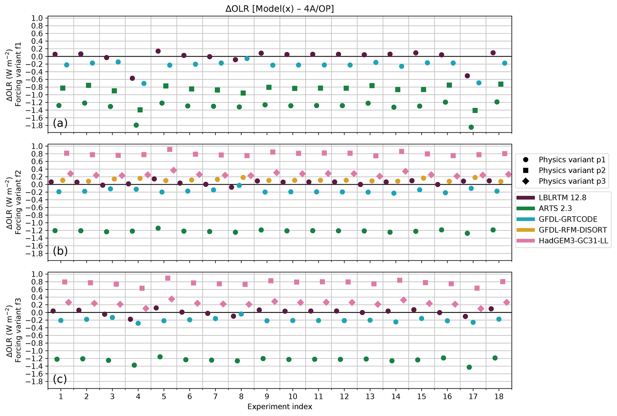
Figure A1Means and standard deviations of OLR differences (model minus 4A/OP; W m−2) as a function of the experiment index. The five models compared to 4A/OP are represented by colors. The three forcing indices f1, f2, and f3 are respectively represented in individual panels (a–c). The different physics variants are differentiated with marker shapes.
Table A1List of atmospheric conditions and gas concentrations defining the 18 experiment variants of RFMIP.
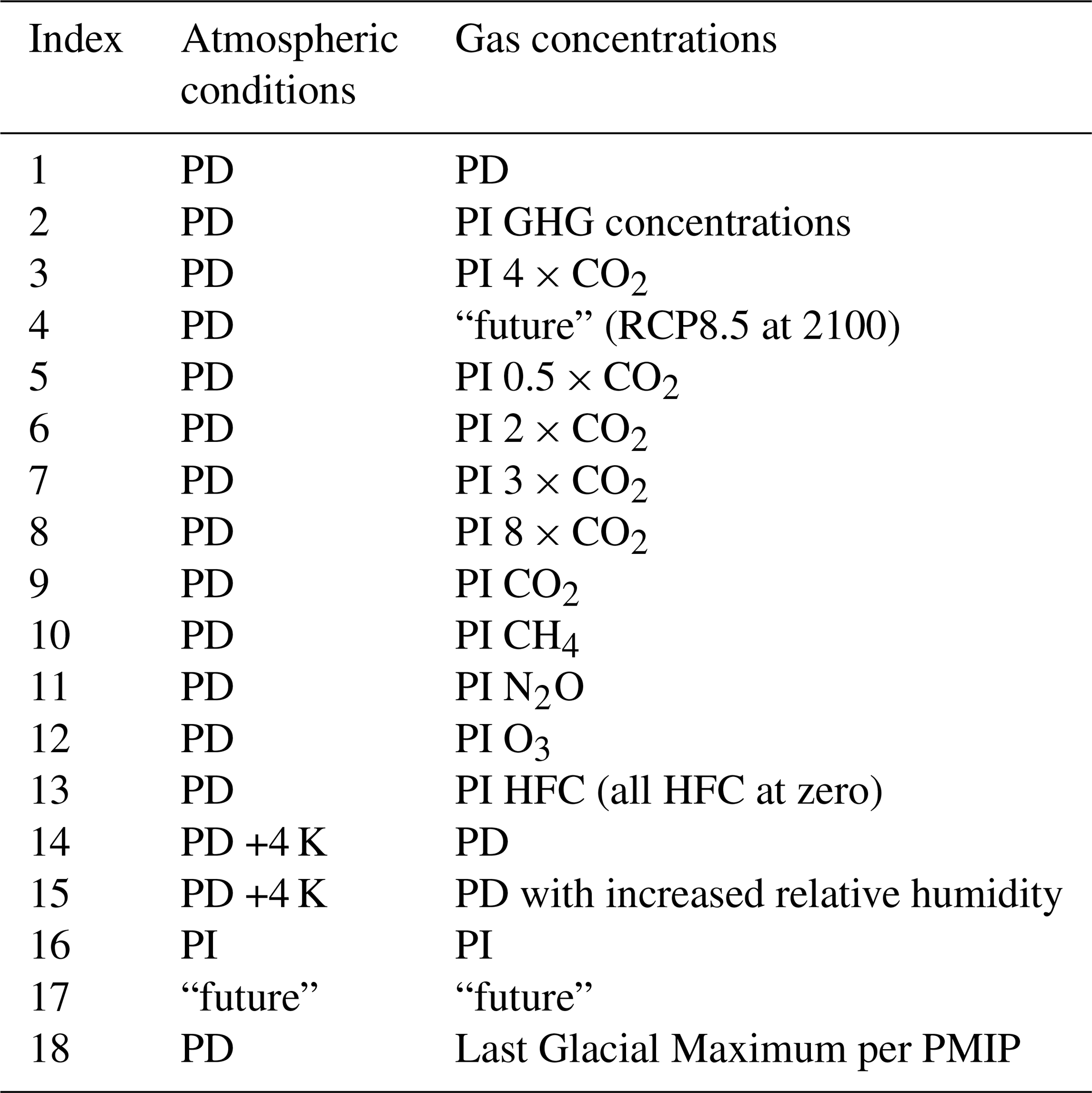
Note: for a complete presentation, please refer to the protocol paper of RFMIP (Pincus et al., 2016); PMIP stands for Paleoclimate Modelling Intercomparison Project (Kageyama et al., 2016).
As discussed in the main discussion, the 4A/OP model is especially close to the results of LBLRTM for the three forcing indices. We notice here that in terms of OLR, the three models GFDL-GRTCODE, LBLRTM, and 4A/OP are close together. The distance between 4A/OP OLR is higher for the forcing variant f1 and experiments 4 and 17 that correspond to “future” gas concentrations. The OLR computed with 4A/OP is significantly higher due to the limited gas list that has been accounted for in the simulation (16 out of the 43 specified in the RFMIP database). These minor gases have a small impact on the pre-industrial and present-day radiative forcing but play a greater part in the future radiative forcing. The concentration of some of these gases increases by orders of magnitude in the future scenario compared to the present-day situation. The difference completely disappears for forcing variants f2 and f3 for which the same ensemble of gases has been considered for all models. Gases that are neglected in the present-day forcing can play an important part in the future forcing as their concentrations increase and should thus be accounted for in such cases. If we exclude experiments 4 and 17 as well as ARTS physics variant p1 that does not include CO2 line mixing, the difference between 4A/OP and other models never exceeds ± 1 W m−2.
The distributed version of the 4A/OP radiative transfer model version 1.5 is available at https://4aop.aeris-data.fr/ (last access: 12 June 2022). This version of 4A/OP does not include the 4A-Flux module version 1.0 yet. However, the development version of 4A/OP v1.5 including 4A-Flux v1.0 – described in this paper – is available on the Zenodo platform (https://doi.org/10.5281/zenodo.5667737; Tellier et al., 2021). The spectroscopic database GEISA (Gestion et Etude des Informations Spectroscopiques Atmosphériques: Management and Study of Atmospheric Spectroscopic Information) is available at https://geisa.aeris-data.fr/ (last access: 12 June 2022). The Thermodynamic Initial Guess Retrieval (TIGR) atmospheric database is available at https://ara.lmd.polytechnique.fr/index.php?page=tigr (last access: 12 June 2022). All inputs and results for the RFMIP experiment rad-irf are available from the Earth System Grid Federation at https://esgf-node.llnl.gov/search/cmip6/ (last access: 12 June 2022). Input data are referenced as https://doi.org/10.22033/ESGF/CMIP6.6320 (Pincus, 2019) and results data used for the calculations in Sect. 3 are referenced as follows: 4A/OP v1.5 (https://doi.org/10.22033/ESGF/CMIP6.12369; Boucher et al., 2020), ARTS 2.3 (https://doi.org/10.22033/ESGF/CMIP6.8919; Brath, 2019), GRTCODE (https://doi.org/10.22033/ESGF/CMIP6.10708; Paynter et al., 2018a), RFM-DISORT (https://doi.org/10.22033/ESGF/CMIP6.10709; Paynter et al., 2018b), HadGEM3-GC3.1 (https://doi.org/10.22033/ESGF/CMIP6.6320; Andrews, 2019), and LBLRTM 12.8 (https://doi.org/10.22033/ESGF/CMIP6.2528; Mlawer and Pernak, 2019).
YT developed and implemented the 4A-Flux module and handled the different applications with fruitful inputs from all authors. CC supervised the whole work and, along with all authors, provided both scientific and technical expertise. JLD also made the participation in RFMIP-IRF possible. YT prepared the paper with contributions from all authors.
The contact author has declared that neither they nor their co-authors have any competing interests.
Publisher's note: Copernicus Publications remains neutral with regard to jurisdictional claims in published maps and institutional affiliations.
Authors acknowledge Robert Pincus for the fruitful collaboration on RFMIP project along with all the teams that have contributed to RFMIP-IRF and publicly provided their model outputs used in this work. We acknowledge the World Climate Research Programme, which, through its Working Group on Coupled Modelling, coordinated and promoted CMIP6. We thank the climate modeling groups for producing and making available their model output, the Earth System Grid Federation (ESGF) for archiving the data and providing access, and the multiple funding agencies who support CMIP6 and ESGF. Further acknowledgements are expressed to the IPSL and the support team of Climserv (the computation cluster of the IPSL) for the provision of both the computational power and the technical support that have been necessary to the completion of this work.
This research has been supported by CNES, CNRS, and Ecole Polytechnique. Yoann Tellier has been funded by Thales and CNES in the framework of scientific collaboration with Institut Polytechnique de Paris doctoral school.
This paper was edited by Volker Grewe and reviewed by two anonymous referees.
Achard, V.: Trois problèmes clés de l'analyse 3D de la structure thermodynamique de l'atmosphère par satellite: Mesure du contenu en ozone; classification des masses d'air; modélisation hyper rapide du transfert radiatif, PhD thesis, Université Paris VI, LMD, Ecole Polytechnique, 91128 Palaiseau CEDEX, France, 1991. a, b
Alvarado, M. J., Payne, V. H., Mlawer, E. J., Uymin, G., Shephard, M. W., Cady-Pereira, K. E., Delamere, J. S., and Moncet, J.-L.: Performance of the Line-By-Line Radiative Transfer Model (LBLRTM) for temperature, water vapor, and trace gas retrievals: recent updates evaluated with IASI case studies, Atmos. Chem. Phys., 13, 6687–6711, https://doi.org/10.5194/acp-13-6687-2013, 2013. a
Andrews, T.: MOHC HadGEM3-GC31-LL model output prepared for CMIP6 RFMIP rad-irf. Version 20191030, WCRP [data set], https://doi.org/10.22033/ESGF/CMIP6.6320, 2019. a
Boucher, O., Denvil, S., Levavasseur, G., Cozic, A., Caubel, A., Foujols, M.-A., Meurdesoif, Y., Dufresne, J.-L., Sima, A., and Tellier, Y.: IPSL 4AOP-v1-5 model output prepared for CMIP6 RFMIP rad-irf. Version 20200611, WCRP [data set], https://doi.org/10.22033/ESGF/CMIP6.12369, 2020. a
Brath, M.: UHH ARTS2.3 model output prepared for CMIP6 RFMIP rad-irf. Version 20190620, WCRP [data set], https://doi.org/10.22033/ESGF/CMIP6.8919, 2019. a
Buehler, S. A., von Engeln, A., Brocard, E., John, V. O., Kuhn, T., and Eriksson, P.: Recent developments in the line-by-line modeling of outgoing longwave radiation, J. Quant. Spectrosc. Ra., 98, 446–457, https://doi.org/10.1016/j.jqsrt.2005.11.001, 2006. a, b
Buehler, S. A., Mendrok, J., Eriksson, P., Perrin, A., Larsson, R., and Lemke, O.: ARTS, the Atmospheric Radiative Transfer Simulator – version 2.2, the planetary toolbox edition, Geosci. Model Dev., 11, 1537–1556, https://doi.org/10.5194/gmd-11-1537-2018, 2018. a, b
Cheruy, F., Scott, N. A., Armante, R., Tournier, B., and Chedin, A.: Contribution to the development of radiative transfer models for high spectral resolution observations in the infrared, J. Quant. Spectrosc. Ra., 53, 597–611, https://doi.org/10.1016/0022-4073(95)00026-H, 1995. a, b
Chevallier, F., Chéruy, F., Scott, N. A., and Chédin, A.: A Neural Network Approach for a Fast and Accurate Computation of a Longwave Radiative Budget, J. Appl. Meteorol., 37, 1385–1397, https://doi.org/10.1175/1520-0450(1998)037<1385:ANNAFA>2.0.CO;2, 1998. a, b
Chevallier, F., Chéruy;, F., Armante, R., Stubenrauch, C. J., and Scott, N. A.: Retrieving the Clear-Sky Vertical Longwave Radiative Budget from TOVS: Comparison of a Neural Network–Based Retrieval and a Method Using Geophysical Parameters, J. Appl. Meteorol., 39, 1527–1543, https://doi.org/10.1175/1520-0450(2000)039<1527:RTCSVL>2.0.CO;2, 2000. a
Chédin, A., Scott, N. A., Wahiche, C., and Moulinier, P.: The Improved Initialization Inversion Method: A High Resolution Physical Method for Temperature Retrievals from Satellites of the TIROS-N Series, J. Appl. Meteorol., 24, 128–143, https://doi.org/10.1175/1520-0450(1985)024<0128:TIIIMA>2.0.CO;2, 1985. a
Chédin, A., Scott, N. A., Husson, N., Flobert, J., Levy, C., and Moine, P.: Satellite meteorology and atmospheric spectroscopy. Recent progress in earth remote sensing from the satellites of the Tiros-N series., J. Quant. Spect. Ra., 40, 257–273, https://doi.org/10.1016/0022-4073(88)90119-7, 1988. a
Chédin, A., Scott, N. A., Claud, C., Bonnet, B., Escobar, J., Dardaillon, S., Cheruy, F., and Husson, N.: Global scale observation of the earth for climate studies, Adv. Space Res., 14, 155–159, https://doi.org/10.1016/0273-1177(94)90364-6, 1994. a
Chéruy, F., Chevallier, F., Morcrette, J.-J., Scott, N. A., and Chédin, A.: A fast method using neural networks for computing the vertical distribution of the thermal component of the Earth radiative budget, C. R. Acad. Sci. Paris, 322, série II, 665–672, 1996. a
Clough, S. A. and Iacono, M. J.: Line-by-line calculation of atmospheric fluxes and cooling rates: 2. Application to carbon dioxide, ozone, methane, nitrous oxide and the halocarbons, J. Geophys. Res.-Atmos., 100, 16519–16535, https://doi.org/10.1029/95JD01386, 1995. a, b
Clough, S. A., Iacono, M. J., and J.-L., M.: Line-by-Line Calculations of Atmospheric Fluxes and Cooling Rates: Application to Water Vapor, J. Geophys. Res., 97, 15761–15785, https://doi.org/10.1029/92JD01419, 1992. a, b
Clough, S. A., Shephard, M. W., Mlawer, E. J., Delamere, J. S., Iacono, M. J., Cady-Pereira, K., Boukabara, S., and Brown, P. D.: Atmospheric radiative transfer modeling: a summary of the AER codes, J. Quant. Spectrosc. Ra., 91, 233–244, https://doi.org/10.1016/j.jqsrt.2004.05.058, 2005. a, b
Delahaye, T., Armante, R., Scott, N. A., Jacquinet-Husson, N., Chédin, A., Crépeau, L., Crevoisier, C., Douet, V., Perrin, A., Barbe, A., Boudon, V., Campargue, A., Coudert, L. H., Ebert, V., Flaud, J.-M., Gamache, R. R., Jacquemart, D., Jolly, A., Kwabia Tchana, F., Kyuberis, A., Li, G., Lyulin, O. M., Manceron, L., Mikhailenko, S., Moazzen-Ahmadi, N., Müller, H. S. P., Naumenko, O. V., Nikitin, A., Perevalov, V. I., Richard, C., Starikova, E., Tashkun, S. A., Tyuterev, V. G., Vander Auwera, J., Vispoel, B., Yachmenev, A., and Yurchenko, S.: The 2020 edition of the GEISA spectroscopic database, J. Molecul. Spectrosc., 380, 111510, https://doi.org/10.1016/j.jms.2021.111510, 2021. a
Dogniaux, M., Crevoisier, C., Armante, R., Capelle, V., Delahaye, T., Cassé, V., De Mazière, M., Deutscher, N. M., Feist, D. G., Garcia, O. E., Griffith, D. W. T., Hase, F., Iraci, L. T., Kivi, R., Morino, I., Notholt, J., Pollard, D. F., Roehl, C. M., Shiomi, K., Strong, K., Té, Y., Velazco, V. A., and Warneke, T.: The Adaptable 4A Inversion (5AI): description and first retrievals from Orbiting Carbon Observatory-2 (OCO-2) observations, Atmos. Meas. Tech., 14, 4689–4706, https://doi.org/10.5194/amt-14-4689-2021, 2021. a
Dudhia, A.: The Reference Forward Model (RFM), J. Quant. Spectrosc. Ra., 186, 243–253, https://doi.org/10.1016/j.jqsrt.2016.06.018, 2017. a, b
Edwards, J. M. and Slingo, A.: Studies with a flexible new radiation code. I: Choosing a configuration for a large-scale model, Q. J. Roy. Meteor. Soc., 122, 689–719, https://doi.org/10.1002/qj.49712253107, 1996. a
Eriksson, P., Buehler, S. A., Davis, C. P., Emde, C., and Lemke, O.: ARTS, the atmospheric radiative transfer simulator, version 2, J. Quant. Spectrosc. Ra., 112, 1551–1558, https://doi.org/10.1016/j.jqsrt.2011.03.001, 2011. a
Eyring, V., Bony, S., Meehl, G. A., Senior, C. A., Stevens, B., Stouffer, R. J., and Taylor, K. E.: Overview of the Coupled Model Intercomparison Project Phase 6 (CMIP6) experimental design and organization, Geosci. Model Dev., 9, 1937–1958, https://doi.org/10.5194/gmd-9-1937-2016, 2016. a, b
Feigelson, E. M., Fomin, B. A., Gorchakova, I. A., Rozanov, E. V., Timofeyev, Y. M., Trotsenko, A. N., and Schwarzkopf, M. D.: Calculation of longwave radiation fluxes in atmospheres, J. Geophys. Res.-Atmos., 96, 8985–9001, https://doi.org/10.1029/91JD00449, 1991. a
Hartmann, D. L., Ramanathan, V., Berroir, A., and Hunt, G. E.: Earth Radiation Budget data and climate research, Rev. Geophys., 24, 439–468, https://doi.org/10.1029/RG024i002p00439, 1986. a
Huang, Y., Ramaswamy, V., and Soden, B.: An investigation of the sensitivity of the clear-sky outgoing longwave radiation to atmospheric temperature and water vapor, J. Geophys. Res.-Atmos., 112, D05104, https://doi.org/10.1029/2005JD006906, 2007. a
Jacquinet-Husson, N., Arié, E., Ballard, J., Barbe, A., Bjoraker, G., Bonnet, B., Brown, L. R., Camy-Peyret, C., Champion, J. P., Chédin, A., Chursin, A., Clerbaux, C., Duxbury, G., Flaud, J. M., Fourrié, N., Fayt, A., Graner, G., Gamache, R., Goldman, A., Golovko, V., Guelachvili, G., Hartmann, J. M., Hilico, J. C., Hillman, J., Lefèvre, G., Lellouch, E., Mikhaïlenko, S. N., Naumenko, O. V., Nemtchinov, V., Newnham, D. A., Nikitin, A., Orphal, J., Perrin, A., Reuter, D. C., Rinsland, C. P., Rosenmann, L., Rothman, L. S., Scott, N. A., Selby, J., Sinitsa, L. N., Sirota, J. M., Smith, A. M., Smith, K. M., Tyuterev, V. G., Tipping, R. H., Urban, S., Varanasi, P., and Weber, M.: The 1997 Spectroscopic GEISA Databank, J. Quant. Spectrosc. Ra., 62, 205–254, https://doi.org/10.1016/S0022-4073(98)00111-3, 1999. a
Jacquinet-Husson, N., Armante, R., Scott, N. A., Chédin, A., Crépeau, L., Boutammine, C., Bouhdaoui, A., Crevoisier, C., Capelle, V., Boonne, C., Poulet-Crovisier, N., Barbe, A., Chris Benner, D., Boudon, V., Brown, L. R., Buldyreva, J., Campargue, A., Coudert, L. H., Devi, V. M., Down, M. J., Drouin, B. J., Fayt, A., Fittschen, C., Flaud, J.-M., Gamache, R. R., Harrison, J. J., Hill, C., Hodnebrog, Ø., Hu, S.-M., Jacquemart, D., Jolly, A., Jiménez, E., Lavrentieva, N. N., Liu, A.-W., Lodi, L., Lyulin, O. M., Massie, S. T., Mikhailenko, S., Müller, H. S. P., Naumenko, O. V., Nikitin, A., Nielsen, C. J., Orphal, J., Perevalov, V. I., Perrin, A., Polovtseva, E., Predoi-Cross, A., Rotger, M., Ruth, A. A., Yu, S. S., Sung, K., Tashkun, S. A., Tennyson, J., Tyuterev, V. G., Vander Auwera, J., Voronin, B. A., and Makie, A.: The 2015 edition of the GEISA spectroscopic database, J. Molecul. Spectrosc., 327, 31–72, https://doi.org/10.1016/j.jms.2016.06.007, 2016. a, b
Jeevanjee, N. and Fueglistaler, S.: Simple Spectral Models for Atmospheric Radiative Cooling, J. Atmos. Sci., 77, 479–497, https://doi.org/10.1175/JAS-D-18-0347.1, 2020. a, b, c
Jeevanjee, N., Seeley, J. T., Paynter, D., and Fueglistaler, S.: An Analytical Model for Spatially Varying Clear-Sky CO2 Forcing, J. Climate, 34, 9463–9480, https://doi.org/10.1175/JCLI-D-19-0756.1, 2021. a
Kageyama, M., Braconnot, P., Harrison, S. P., Haywood, A. M., Jungclaus, J. H., Otto-Bliesner, B. L., Peterschmitt, J.-Y., Abe-Ouchi, A., Albani, S., Bartlein, P. J., Brierley, C., Crucifix, M., Dolan, A., Fernandez-Donado, L., Fischer, H., Hopcroft, P. O., Ivanovic, R. F., Lambert, F., Lunt, D. J., Mahowald, N. M., Peltier, W. R., Phipps, S. J., Roche, D. M., Schmidt, G. A., Tarasov, L., Valdes, P. J., Zhang, Q., and Zhou, T.: The PMIP4 contribution to CMIP6 – Part 1: Overview and over-arching analysis plan, Geosci. Model Dev., 11, 1033–1057, https://doi.org/10.5194/gmd-11-1033-2018, 2018. a
Lamouroux, J., Régalia, L., Thomas, X., Vander Auwera, J., Gamache, R. R., and Hartmann, J.-M.: CO2 line-mixing database and software update and its tests in the 2.1 µm and 4.3 µm regions, J. Quant. Spectrosc. Ra., 151, 88–96, https://doi.org/10.1016/j.jqsrt.2014.09.017, 2015. a, b
Liou, K. N.: An Introduction to Atmospheric Radiation (second edition), International Geophysics Series, vol. 84, Academic Press, London UK, December 2002. a
Luther, F. M., Ellingson, R. G., Fouquart, Y., Fels, S., Scott, N. A., and Wiscombe, W. J.: Intercomparison of Radiation Codes in Climate Models (ICRCCM): longwave clear sky results., B. Am. Meteorol. Soc., 69, 40–48, https://doi.org/10.1175/1520-0477-69.1.40, 1988. a
Meinshausen, M., Vogel, E., Nauels, A., Lorbacher, K., Meinshausen, N., Etheridge, D. M., Fraser, P. J., Montzka, S. A., Rayner, P. J., Trudinger, C. M., Krummel, P. B., Beyerle, U., Canadell, J. G., Daniel, J. S., Enting, I. G., Law, R. M., Lunder, C. R., O'Doherty, S., Prinn, R. G., Reimann, S., Rubino, M., Velders, G. J. M., Vollmer, M. K., Wang, R. H. J., and Weiss, R.: Historical greenhouse gas concentrations for climate modelling (CMIP6), Geoscientific Model Development, 10, 2057–2116, https://doi.org/10.3929/ethz-b-000191830, 2017. a, b
Mlawer, E. and Pernak, R.: AER LBLRTM model output prepared for CMIP6 RFMIP rad-irf. Version 20190517, WCRP [data set], https://doi.org/10.22033/ESGF/CMIP6.2528, 2019. a
Mlawer, E. J., Payne, V. H., Moncet, J.-L., Delamere, J. S., Alvarado, M. J., and Tobin, D. C.: Development and recent evaluation of the MT_CKD model of continuum absorption, Philos. T. R. Soc. A, 370, 2520–2556, https://doi.org/10.1098/rsta.2011.0295, 2012. a
Mlynczak, M. G., Daniels, T. S., Kratz, D. P., Feldman, D. R., Collins, W. D., Mlawer, E. J., Alvarado, M. J., Lawler, J. E., Anderson, L. W., Fahey, D. W., Hunt, L. A., and Mast, J. C.: The spectroscopic foundation of radiative forcing of climate by carbon dioxide, Geophys. Res. Lett., 43, 5318–5325, https://doi.org/10.1002/2016GL068837, 2016. a
Paynter, D. J., Menzel, R., Freidenreich, S., Schwarzkopf, D. M., Jones, A., Wright, G., and Rand, K.: NOAA-GFDL GFDL-GRTCODE model output prepared for CMIP6 RFMIP rad-irf. Version 20180701, WCRP [data set], https://doi.org/10.22033/ESGF/CMIP6.10708, 2018a. a
Paynter, D. J., Menzel, R., Freidenreich, S., Schwarzkopf, D. M., Jones, A., Wright, G., and Rand, K.: NOAA-GFDL GFDL-RFM-DISORT model output prepared for CMIP6 RFMIP rad-irf. Version 20180701, WCRP [data set], https://doi.org/10.22033/ESGF/CMIP6.10709, 2018b. a
Pincus, R.: input4MIPs.CMIP6.RFMIP.UColorado.UColorado-RFMIP-1-2. Version: 20190401, WCRP [data set], https://doi.org/10.22033/ESGF/input4MIPs.10421, 2019. a
Pincus, R., Forster, P. M., and Stevens, B.: The Radiative Forcing Model Intercomparison Project (RFMIP): experimental protocol for CMIP6, Geosci. Model Dev., 9, 3447–3460, https://doi.org/10.5194/gmd-9-3447-2016, 2016. a, b, c, d
Pincus, R., Buehler, S. A., Brath, M., Crevoisier, C., Jamil, O., Evans, K. F., Manners, J., Menzel, R. L., Mlawer, E. J., Paynter, D., Pernak, R. L., and Tellier, Y.: Benchmark Calculations of Radiative Forcing by Greenhouse Gases, J. Geophys. Res.-Atmos., 125, https://doi.org/10.1029/2020jd033483, 2020. a, b, c, d, e
Ridgway, W. L., Harshvardhan, and Arking, A.: Computation of atmospheric cooling rates by exact and approximate methods, J. Geophys. Res.-Atmos., 96, 8969–8984, https://doi.org/10.1029/90JD01858, 1991. a, b, c
Rothman, L. S., Gordon, I. E., Babikov, Y., Barbe, A., Chris Benner, D., Bernath, P. F., Birk, M., Bizzocchi, L., Boudon, V., Brown, L. R., Campargue, A., Chance, K., Cohen, E. A., Coudert, L. H., Devi, V. M., Drouin, B. J., Fayt, A., Flaud, J.-M., Gamache, R. R., Harrison, J. J., Hartmann, J.-M., Hill, C., Hodges, J. T., Jacquemart, D., Jolly, A., Lamouroux, J., Le Roy, R. J., Li, G., Long, D. A., Lyulin, O. M., Mackie, C. J., Massie, S. T., Mikhailenko, S., Müller, H. S. P., Naumenko, O. V., Nikitin, A. V., Orphal, J., Perevalov, V., Perrin, A., Polovtseva, E. R., Richard, C., Smith, M. A. H., Starikova, E., Sung, K., Tashkun, S., Tennyson, J., Toon, G. C., Tyuterev, V. G., and Wagner, G.: The HITRAN2012 molecular spectroscopic database, J. Quant. Spectrosc. Ra., 130, 4–50, https://doi.org/10.1016/j.jqsrt.2013.07.002, 2013. a
Schuster, A.: Radiation Through a Foggy Atmosphere, Astrophys. J., 21, 1, https://doi.org/10.1086/141186, 1905. a
Scott, N. A.: A direct method of computation of the transmission function of an inhomogeneous gaseous medium – I: Description of the method, J. Quant. Spectrosc. Ra., 14, 691–704, https://doi.org/10.1016/0022-4073(74)90116-2, 1974. a
Scott, N. A. and Chedin, A.: A Fast Line-by-Line Method for Atmospheric Absorption Computations: The Automatized Atmospheric Absorption Atlas, J. Appl. Meteorol., 20, 802–812, https://doi.org/10.1175/1520-0450(1981)020<0802:AFLBLM>2.0.CO;2, 1981. a, b, c
Stamnes, K., Thomas, G. E., and Stamnes, J. J.: Radiative Transfer in the Atmosphere and Ocean, 2 edn., https://doi.org/10.1017/9781316148549, Cambridge University Press, 2017. a, b
Tellier, Y., Crevoisier, C., Armante, R., Dufresne, J.-L., and Meilhac, N.: 4A-Flux v1.0: the radiative flux and heating rate module integrated into 4A/OP v1.5 radiative transfer code, Zenodo [code], https://doi.org/10.5281/zenodo.5667737, 2021. a
Tournier, B., Armante, R., and Scott, N. A.: Stransac-93, 4A-93. Développement et validation des nouvelles versions des codes de transfert radiatif pour application au projet IASI, Internal Rep. LMD, No. 201, LMD/CNRS, Ecole Polytechnique, Palaiseau, France, 1995. a
Trenberth, K. E., Fasullo, J. T., and Kiehl, J.: Earth's Global Energy Budget, B. Am. Meteorol. Soc., 90, 311–324, https://doi.org/10.1175/2008BAMS2634.1, 2009. a
Walters, D., Baran, A. J., Boutle, I., Brooks, M., Earnshaw, P., Edwards, J., Furtado, K., Hill, P., Lock, A., Manners, J., Morcrette, C., Mulcahy, J., Sanchez, C., Smith, C., Stratton, R., Tennant, W., Tomassini, L., Van Weverberg, K., Vosper, S., Willett, M., Browse, J., Bushell, A., Carslaw, K., Dalvi, M., Essery, R., Gedney, N., Hardiman, S., Johnson, B., Johnson, C., Jones, A., Jones, C., Mann, G., Milton, S., Rumbold, H., Sellar, A., Ujiie, M., Whitall, M., Williams, K., and Zerroukat, M.: The Met Office Unified Model Global Atmosphere 7.0/7.1 and JULES Global Land 7.0 configurations, Geosci. Model Dev., 12, 1909–1963, https://doi.org/10.5194/gmd-12-1909-2019, 2019. a
Wiscombe, W. J.: Extension of the doubling method to inhomogeneous sources, J. Quant. Spectrosc. Ra., 16, 477–489, https://doi.org/10.1016/0022-4073(76)90083-2, 1976. a
Gestion et Étude des Informations Spectroscopiques Atmosphériques (Management and Study of Spectroscopic Information).
High Resolution Transmission.
For clarity purposes, the dependence on the wavenumber ν [unit: cm−1] is not mentioned explicitly in variable names. For instance, where we should have written , we simply write F↓(σ). All variables referred to as monochromatic follow the same notation convention.
RFMIP website: https://rfmip.leeds.ac.uk/ (last access: 12 June 2022).
The gases that have been taken into account in 4A/OP simulations for forcing variant f1 are H2O, O3, CO2, CH4, N2O, CO, O2, N2, CH3Cl, SF6, CFC-11, CFC-12, CCl4, CFC-113, HCFC-22, and HFC-134a.
- Abstract
- Introduction
- Implementation of 4A-Flux into the 4A/OP radiative transfer model
- Evaluation of 4A-Flux over the RFMIP database
- Sensitivity of radiative fluxes and vertical heating rate to temperature and composition
- Conclusions
- Appendix A: Complementary information on the evaluation of 4A-Flux over the RFMIP database
- Code and data availability
- Author contributions
- Competing interests
- Disclaimer
- Acknowledgements
- Financial support
- Review statement
- References