the Creative Commons Attribution 4.0 License.
the Creative Commons Attribution 4.0 License.
 | 23 Jun 2022
An online ensemble coupled data assimilation capability for the Community Earth System Model: system design and evaluation
Jingzhe Sun
Yingjing Jiang
Shaoqing Zhang
Weimin Zhang
Lv Lu
Guangliang Liu
Yuhu Chen
Xiang Xing
Xiaopei Lin
Lixin Wu
The Community Earth System Model (CESM) developed by the National Center for Atmospheric Research (NCAR) has been used worldwide for climate studies. This study extends the efforts of CESM development to include an online (i.e., in-core) ensemble coupled data assimilation system (CESM-ECDA) to enhance CESM's capability for climate predictability studies and prediction applications. The CESM-ECDA system consists of an online atmospheric data assimilation (ADA) component implemented in both the finite-volume and spectral-element dynamical cores and an online ocean data assimilation (ODA) component. In ADA, surface pressures (Ps) are assimilated, while in ODA, gridded sea surface temperature (SST) and ocean temperature and salinity profiles at real Argo locations are assimilated. The system has been evaluated within a perfect twin experiment framework, showing significantly reduced errors of the model atmosphere and ocean states through “observation” constraints by ADA and ODA. The weakly coupled data assimilation (CDA) in which both the online ADA and ODA are conducted during the coupled model integration shows smaller errors of air–sea fluxes than the single ADA and ODA, facilitating the future utilization of cross-covariance between the atmosphere and ocean at the air–sea interface. A 3-year CDA reanalysis experiment is also implemented by assimilating Ps, SST and ocean temperature and salinity profiles from the real world spanning the period 1978 to 1980 using 12 ensemble members. The success of the online CESM-ECDA system is the first step to implementing a high-resolution long-term climate reanalysis once the algorithm efficiency is much improved.
- Article
(20263 KB) - Full-text XML
- BibTeX
- EndNote


The author's copyright for this publication is transferred to Ocean University of China.
The Community Earth System Model (CESM) is a fully coupled global Earth system model developed by the National Center for Atmospheric Research (NCAR), consisting of several geophysical component models (atmosphere, ocean, land, land ice, sea ice, river runoff, and ocean wave) and a central infrastructure for coupling component models. It can simulate the past, present, and future climate states of the Earth system (e.g., Chiodo et al., 2016; Glotfelty et al., 2017; Chang et al., 2020) and has been used worldwide in numerous climate studies (e.g., Goldenson et al., 2012; Cheng et al., 2014; Gantt et al., 2014; Fasullo and Nerem, 2016) to study the evolution mechanisms of climate and environment (e.g., Goosse and Holland, 2005; Bitz, 2008; Chandan and Peltier, 2018), the impact of natural processes and human activities on climate change, and the prediction of climate change (e.g., Coelho and Goddard, 2009; Arblaster et al., 2011; Asefi-Najafabady et al., 2018).
Developing coupled data assimilation (CDA) is an inevitable requirement to improve initialization, state estimation, and prediction of coupled models with observations available in multiple components of the Earth system (Zhang et al., 2020b). Traditionally, data assimilation (DA) is carried out independently in an uncoupled model, such as assimilating atmospheric observations into an atmosphere component model or assimilating oceanic observations into an ocean component model, which is referred to as uncoupled DA (Derber and Rosati, 1989; Rosati et al., 1997; Saha et al., 2006; Balmaseda and Anderson, 2009). When the uncoupled DA is used to initialize the coupled model integration, it is necessary to first combine the single-component analyses obtained independently from the single-component DA to form the coupled initial conditions for the coupled model. With the wide application of coupled models in the study of weather and climate systems, the demand for CDA is rising rapidly (Penny et al., 2017). CDA refers to the joint assimilation of observations in different component systems and allows observational information to be transferred and exchanged among different components dynamically and statistically (e.g., Lu et al., 2015; Zhang et al., 2020b). It has been shown that CDA is able to improve the interannual climate prediction skills of coupled models (e.g., Collins, 2002; Zhang et al., 2010). Therefore, CDA is considered an effective method for the initialization of multi-component coupled Earth system models and the production of coupled reanalysis (Zhang, 2011).
As described by Penny et al. (2017), CDA can be broadly categorized into two approaches: weakly CDA (WCDA) and strongly CDA (SCDA). WCDA is defined by the fact that the coupling occurs during the forecast stage using a coupled forecast model as DA is ongoing. WCDA assimilates the observations into the corresponding single model component of the coupled model system and then transfers the observational information to other model components through flux exchange of the coupled model. The second approach, SCDA, uses the cross-covariance of model components to directly assimilate the observations of an Earth system component into other coupled model components. The advantage of SCDA is that observations at a given time have instantaneous impacts across all components during all available analyses (Penny et al., 2017; Zhang et al., 2020b). Due to the difficulties in obtaining a high signal-to-noise ratio of the covariance between model components (Han et al., 2013), by now the WCDA is still the common choice for assimilating observations into coupled models (e.g., Laloyaux et al., 2016; Browne et al., 2019; Skachko et al., 2019; Tang et al., 2020; Mu et al., 2020), and meanwhile some studies have also discussed the SCDA (e.g., Penny et al., 2017). In this study, we use WCDA.
According to the mode of data transfer between the numerical model and assimilation algorithm, ensemble-based CDA can be divided into two categories: offline CDA and online CDA. In offline CDA, data are transferred between the model ensemble and assimilation algorithm through data reading and writing. The data assimilation research test bed (DART; Anderson et al., 2009) developed by NCAR and the Gridpoint Statistical Interpolation (GSI) ensemble Kalman filter (EnKF) system (Kleist et al., 2009) released by the Developmental Testbed Center (DTC) are both based on an offline mode. Although the offline CDA is a convenient way to implement a CDA procedure on a relatively short scale, and the majority of the I/O cost in DART is low compared to the total time (Karspeck et al., 2018), an online CDA system is more efficient and necessary for climate studies. The online CDA is usually realized by integrating a numerical model and DA algorithm into one executable program, so that data exchange between model and assimilation is generally realized by memory management. For example, the ensemble CDA (ECDA) system developed by Zhang et al. (2005, 2007), based on the Geophysical Fluid Dynamics Laboratory (GFDL) coupled climate model, and the Parallel Data Assimilation Framework (PDAF) developed by Nerger and Hiller (2013), based on the fully coupled Alfred Wegener Institute, Helmholtz Center for Polar and Marine Research Climate Model (Mu et al., 2020; Nerger et al., 2020), are online CDA systems.
Extensive offline DA works with CESM have been explored in previous studies (e.g., Anderson et al., 2009; Raeder et al., 2012; Karspeck et al., 2013, 2018). All these studies are based on an offline DA framework which needs to read and write restart files at every assimilating time step. This time-consuming method makes it difficult to produce a long-term climate reanalysis. In order to develop a coupled prediction and climate reanalysis, especially toward the goal of high-resolution CESM (CESM-HR; Zhang et al., 2020a) CDA for HR coupled model prediction initialization and reanalysis, a continuous CDA within CESM is highly desirable, although the DART exists and the next-generation DA system (Joint Center for Satellite Data Assimilation JEDI DA system) is designed and has been under development to replace the GSI and other US agency DA systems. This paper serves as documentation for the initial step of CESM-HR CDA development and the ensemble coupled data assimilation system (CESM-ECDA) design and its performance.
In the filtering algorithm, the DA method used in this study (which is the ensemble adjustment Kalman filter, EAKF) is the same as previous studies (Zhang and Anderson, 2003; Anderson et al., 2009; Karspeck et al., 2018), but we implement the CESM-ECDA as an online CDA system which uses computer memory management to compile the assimilation codes and the model codes into an executable file. Avoiding frequent huge data reading and writing is extremely important to realize efficient climate reanalysis, especially for high-resolution model cases. Although a lot of CESM DA work using DART has been done and a 12-year reanalysis has been presented (Karspeck et al., 2018), longer-term climate reanalysis is still a challenge. Our motivation is to develop an online CESM-ECDA system that can support long-time integration and assimilation in the near future. By that, we can make a series of long-timescale (such as 40-year or even 100-year) climate reanalysis experiments in different resolutions for climate assessment. This study is different from Karspeck et al. (2018) in the following two aspects: (1) the CESM-ECDA system passes data through memory instead of files, and (2) the online DA system within the spectral-element (SE) dynamic-core atmosphere model can support high-resolution simulation.
This paper is organized as follows. Section 2 describes the CGCM (Coupled General Circulation Model) used in this work, the ensemble filtering algorithm, and the perfect twin experiment design for the evaluation. The implementation of the ensemble-based online CESM DA capability is described in Sect. 3. More specifically, Sect. 3.1 describes the atmospheric data assimilation (ADA) system within the Community Atmosphere Model (CAM) using the finite-volume dynamical core (dynamic core; hereafter CAM-FV), Sect. 3.2 describes the ADA system within CAM using the spectral-element dynamic-core CAM (hereafter CAM-SE), and Sect. 3.3 discusses the ocean DA (ODA) system with the Parallel Ocean Program (POP) model. Section 4 describes the establishment and evaluation of online CESM-ECDA system. Finally, summary and discussions are given in Sect. 5.
2.1 Brief description of CESM
The version of CESM used in this work is not the latest version of CESM2 (Danabasoglu et al., 2020) but is based on an earlier version tagged as CESM1.3-beta17_sehires38, which is a version specifically developed to better support high-resolution CESM simulations (Small et al., 2014; Chang et al., 2020). The corresponding component model versions are the CAM version 5 (CAM5; Neale et al., 2012), the POP version 2 (POP2; Smith et al., 2010), the Community Ice Code version 4 (CICE4; Hunke and Lipscomb, 2008), and the Community Land Model version 4 (CLM4; Lawrence et al., 2011).
2.2 Brief summary of EAKF
The ensemble adjustment Kalman filter (EAKF) was first designed by Anderson (2001) followed by some modifications (Anderson, 2003) and immediately applied to comprehensive general circulation models (Zhang and Anderson, 2003; Zhang et al., 2005, 2007). As a popular variant of the traditional ensemble Kalman filter (EnKF; Evensen, 1994, 2003), the EAKF has been widely used in DA research and applications. Compared with the traditional EnKF that randomly perturbs the observations, the advantage of EAKF is that it can retain the higher-order moments (i.e., nonlinear information) in the prior samples (Zhang and Anderson, 2003). The EAKF does not need to perturb observations, thus avoiding the generating of extra noise into the analysis system. Based on a systematic analysis of the existing ensemble filtering algorithms, Tippett et al. (2003) pointed out that the EAKF method is one realization of the ensemble square root filter (EnSRF) and a deterministic filtering algorithm. When the error distribution of each scalar observation is independent of each other, a sequential filtering method can be used to assimilate each scalar observation one by one. When the observation errors are correlated, the singular value decomposition (SVD) can be used to first decorrelate the errors, and then the sequential filtering can be carried out.
As a sequential filter, the EAKF can be conveniently implemented by two steps consisting of two key equations (Anderson, 2001, 2003; Zhang and Rosati, 2010). The first equation computes the observational increment as
where i is the ensemble index, y represents the observable state variable, and σ is the error standard deviation. The superscript p always denotes the prior quantity estimated by the model, and o always denotes the prior quantity estimated by observation. The overbar denotes the ensemble mean. The first term on the right hand is the adjusted ensemble mean, and the second term with the third term on the right hand is called the adjusted ensemble spread.
The second step regresses the observational increment computed by the first step onto the relevant model grids. That can be expressed as
where cov(Δx,Δy) is the covariance, and σy is the standard deviation, which are both evaluated by the model ensemble. Once all observations are looped over all the relevant model variables on the model grids, the analysis step is completed, and the model is initialized for the integration of the next step. For more details, please refer to Zhang and Rosati (2010).
2.3 Twin experiment design
The implementation of CDA is a complex multi-task problem, which involves many factors, such as the coupled model bias, sampling of the observation system, and verification of the analysis scheme. The uncertainty in any of these aspects may make the evaluation of a CDA system very difficult. In order to reduce the uncertainty and the evaluation complexity, a perfect model framework based on pseudo-observations (i.e., the perfect twin experiment) is adopted here to eliminate the influence of model bias and observation system sampling on the assessment of the CDA system. The advantage of the perfect twin experiment design is that the known “truth” can be used as an accurate and reliable reference in evaluating the analysis quality of the CDA system. A similar framework has been used in Browne and Leeuwen (2015) to assess the performance of the equivalent weight filter within a coupled ocean–atmosphere general circulation model. In addition, when new assimilation components or observation types are added into the CDA system, the change of the assimilation performance can be effectively quantified.
In the perfect twin experiment design, a time series of single-member model states are taken as the truth, which can start from an arbitrary date (e.g., denoted as January 1980 in this paper). White noise is then added onto the truth to generate the pseudo-observations assimilated in the analysis stage. Thus, the assimilated observations here are gridded data at the grid points as the model variables. The added white noise is a parameter that determines the intensity of the observational constraint. It is used to account for the random measurement error of the observation system but does not include the representation error reflecting the limitation of the sampling scale. To sufficiently decorrelate the truth and the free integration of the model ensemble (i.e., the control experiment without assimilation of any observations), we use the restart of a 20-model-year free integration as the initial condition of the experiments.
The surface pressure reflects the total air mass of the atmosphere column at a location on the Earth's surface (terrain or ocean). Previous studies (e.g., Whitaker et al., 2004; Anderson et al., 2005; Compo et al., 2006) have emphasized several advantages of using surface pressure observations to produce historical reanalyses. As described in Compo et al. (2006), the surface pressure information through geostrophy can be expected to yield a reasonable approximation to the barotropic part of the flow, which accounts for a substantial part of the total flow. There are usually two approaches to implementing surface pressure assimilation. One is projecting the observational surface pressure increments to three-dimensional atmospheric variables through the geostrophic relationship (Poli et al., 2013). The other is using the ensemble covariance between the surface pressure and other atmospheric variables to adjust the three-dimensional atmosphere (e.g., Compo et al., 2011; Yang et al., 2021). The Twentieth Century Reanalysis (20CR) is the first centurial reanalysis to only assimilate surface pressure observations (Compo et al., 2006). Since then, other reanalysis products have been generated by assimilating mainly surface pressure observations, such as ERA-20C (Poli et al., 2013), 20CRv2c (Compo et al., 2011), 20CRv3 (Slivinski et al., 2019), and GFDL's DCIS (Yang et al., 2021).
Using the covariance of surface pressure to adjust three-dimensional atmospheric variables can increase the observational constraint from surface pressure (Yang et al., 2021), but it often requires a large ensemble size. Here, in order to make the assimilation algorithm more portable and suitable for future high-resolution data assimilation, and considering the development feasibility and efficiency with finite computational resources, we use 12 ensemble members instead of a very large ensemble size as used in 20CR. Such a small-size ensemble may not be suitable to resolve three-dimensional increments of atmospheric variables via the ensemble covariance with surface pressure observation. Although we only assimilate the surface pressure, other three-dimensional variables are also adjusted through a geostrophic relationship and a thermal wind relationship. Further justification will be provided in Sect. 4.2.
The observation assimilated by ADA is surface pressure (Ps), and the standard deviation of the added observation error is 10 hPa; the observations assimilated by ODA are sea surface temperature (SST), three-dimensional temperature, and salinity from in situ ocean profiles which are generated from the truth. The corresponding standard deviations of observation errors are 0.5 K for temperature and 0.1 PSU for salinity at the sea surface (typical error levels for SST and sea surface salinity) and exponentially decay to one-tenth of the surface values at 2000 m depth. These standard deviations have been trialed and adopted in previous similar studies (e.g., Zhang et al., 2007). The in situ ocean profiles are sampled using the real locations of Argo data in 2007.
The ADA assimilation frequency is 6 h, and the ODA is 1 d. As an initial verification of the CESM-ECDA system, we do not directly use a high-resolution experimental setup but use a standard resolution (100 km in ocean and 200 km (100 km) in FV (SE) atmosphere). Following previous studies (Zhang et al., 2005, 2007) on the covariance localization technique, and under computational resource constraint, trial and error is used to determine the ensemble size to be 12 in this perfect model study. And the ensembles of initial conditions are constructed using the atmosphere states of 12 consecutive days.
Referring to the 20CRv2 (Compo et al., 2011), CFSR (NCEP Climate Forecast System Reanalysis; Saha et al., 2010), and CM2.1-ECDA (Zhang et al., 2007), the horizontal localization radius is 2000 km in FV core and 2500 km in SE core in ADA in this work. Referring to Zhang et al. (2007) and Karspeck et al. (2018), the horizontal localization radius of SST observations is set to be 1000 km in ODA. In the vertical direction, SST observations are allowed to affect the ocean temperature of the 10 topmost model levels (100 m depth). The horizontal localization radiuses are 1000 km for temperature profiles and 500 km for salinity profiles. In addition, the horizontal correlation scale is multiplied by a cos(θ) (θ is the grid latitude) factor up to 80∘ N (S) to make the scale consistent with the characteristics of the Rossby deformation radius for a global analysis scheme (for more details, please see Zhang et al., 2005, 2007). Each observation is only allowed to impact at most two neighboring levels (one above and one below), and the deepest profile layer corrects the model values of all layers below.
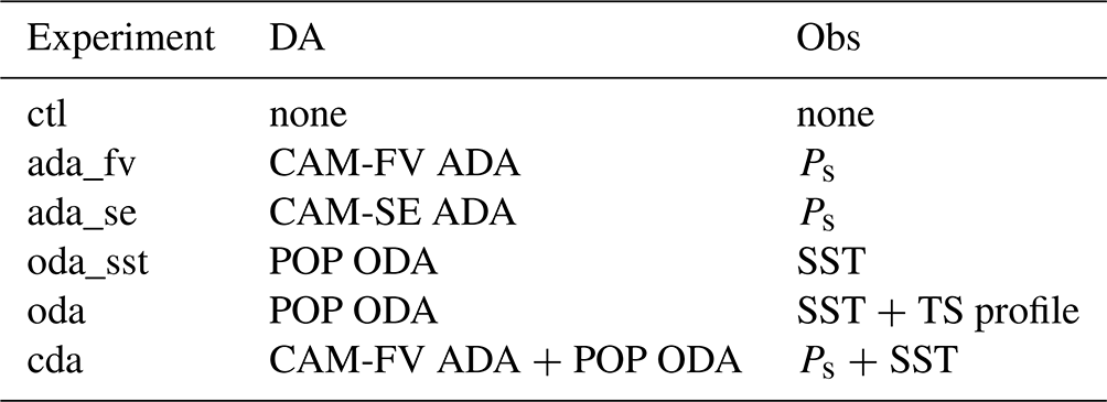
The design of the evaluation experiments for the ADA, ODA, and CDA is shown in Table 1. Given that our main purpose is to document the development of the online CDA system for the community rather than provide reanalysis products, and the constraint of computational resources, we only run 1 model year to verify the reliability of the algorithm in this perfect twin experiment. We can see that the DA in the atmosphere and upper ocean has sufficiently converged. The ensemble experiments include the control experiment (ctl) without assimilating any observations, the ADA experiments which only assimilate the Ps observations with CAM-FV (ada_fv) and CAM-SE (ada_se), the ODA experiments assimilating only the SST observations (oda_sst) and both the SST and in situ ocean profiles of temperature and salinity (TS profile; oda), and the CDA experiment assimilating both the Ps and SST observations with CAM-FV (cda). The experiments' component settings in this study are BHISTC5 (historical run with CAM5) in FV and B1850CN in SE.
The validation of assimilation results is based on the root mean square error (RMSE), which is the most widely used statistic in system evaluation. RMSE is the standard deviation of the prediction errors, which measures how much the simulated data differ from the reference data (i.e., the truth). Since both atmosphere and ocean observations assimilated in this paper are located near the air–sea interface, and in principle, CDA can make more effective use of the observations near the interface and thus improve the coupled state estimation there, this paper mainly analyzes the model variables and fluxes near the interface. The atmosphere model variables near the interface used in this paper include the atmosphere (Ps), surface temperature (Ts), surface wind components (Us and Vs), and surface specific humidity (Qs). The analyzed ocean model variables include SST and ocean subsurface temperature and salinity. The fluxes at the air–sea interface used here include the sensible heat flux (SHF) and the latent heat flux (LHF).
This section describes the framework and implementation of the online DA components of the CESM-ECDA system, which include the ADA components with CAM and the ODA component with POP. The ADA components are implemented in both CAM-FV and CAM-SE.
3.1 ADA with CAM-FV
3.1.1 Online ensemble collection and distribution with CAM-FV data structure
CAM-FV adopts regular latitude–longitude grid in the horizontal direction, and both the model and assimilation are performed in parallel modes. The parallel domain decomposition in the model integration space is realized by dividing the global field in the horizontal direction based on the adjacent geophysical location. During the forecast stage, each processing element (PE) is responsible for a sub-domain of the global field of a single ensemble member, and different ensemble members are completely independent when the model integrated forward. When the model ensemble reaches the analysis time, a “super-parallel” technique (Zhang et al., 2007) is used to transmit the data between the model space and the analysis space. The super-parallel technique allows us to make full use of the available computing resources and enables the model integration and the analysis to be carried out online in an iterative manner.
Online data interaction based on the super-parallel technique mainly includes two stages: online ensemble collection and online ensemble distribution. Online collection refers to the transformation of the parallel domain decomposition and corresponding data storage form of the model space to those of the analysis space. As a result, each PE can obtain the ensemble data required by the ensemble filtering algorithm. Conversely, online distribution indicates the transformation of the domain decomposition and data storage form of the analysis space back to those of the model space. In this way, the updated analysis ensemble can be used as the initial conditions for the model integration of the next assimilation cycle. The transformation between the model space and the analysis space is mainly based on the data collection and distribution functions of the Message Passing Interface (MPI; Gropp et al., 1996), and it is an online data interaction mode via the memory-based reading and writing. An online coupling strategy and implementation of standards using MPI in an ensemble data assimilation system have been detailed in Browne and Wilson (2015).
Figure 1a is an example of the parallel domain decomposition and online collection and distribution with a total of 16 PEs and four ensemble members with CAM-FV. In order to conduct the parallel task decomposition in the analysis space, the global field is divided into 16 PEs of the global PE list. To some extent, the parallel decomposition in the analysis space is arbitrary, while Fig. 1a just shows a global domain decomposition according to a layout with 4×4 PEs. It should be noted that we can also specify other decomposition layout types, such as 2×8 PEs. The halo is 12 grids in our experiments. In theory, the halo should depend on the localization scale. But practically, we choose an appropriate halo according to some previous experiments and model resolutions.

Figure 1(a) The parallel domain decomposition and the online ensemble collection and distribution of a scalar field with CAM-FV. The four ensemble members are integrated forward in time in parallel, using four processors for each member. At analysis time, the ensemble members are synchronized, and the global four-element ensemble vectors are decomposed onto all 16 analysis processors. For each physical field, each analysis processor sequentially uses the observations to update the ensemble vectors at each grid point in its core domain (green) and halo (yellow). Once all nearby observations have been assimilated, the updated ensemble vectors in the core domains are transmitted back to the integration processors, completing the cycle. (b) The parallel domain decomposition and the online ensemble collection and distribution of a scalar field with CAM-SE. Different from CAM-FV, CAM-SE uses the cubed-sphere grid. To address this grid change, the implementation of domain decomposition with CAM-SE adopts a similar fashion to that used in DART (Anderson et al., 2009). This new method allows us to “randomly” assign model states to different PEs. And the calculation of the forward operator is realized based on the MPI2 remote memory access (RMA). At analysis time, the ensemble members are synchronized, and the global ensemble vectors are randomly decomposed onto all eight PEs (grid points with same color in the figure). (c) Schematic of the CESM-ECDA system. During the forecast stage of a DA cycle, ensembles of various components, including CAM and POP, of the CESM system are integrated forward. The atmosphere model and ocean model are dynamically coupled together during the forecast phase (the double arrow between CAM and POP). Taking the atmosphere component as an example, when the analysis time of the atmosphere is reached, the CESM ensemble integration is suspended and the forecast ensemble of CAM is used as the background for the assimilation of the atmospheric observations (the red upward-pointing curved arrow) using the EAKF algorithm (the red solid ellipse). When all the atmospheric observations have been assimilated, the analysis ensemble of CAM is used as the initial conditions of the forecast stage in the next DA cycle (the red downward-pointing curved arrow). The ODA cycle for the POP model is similar and marked as blue in the figure. The ADA and ODA may have the same or different frequencies.
3.1.2 Implementation of sequential EAKF algorithm with CAM-FV
The implementation of the sequential EAKF with CAM-FV uses an approximate algorithm of the compute domain–data domain strategy of Anderson (Anderson, 2001) to parallelize the filter. Figure 2 shows a schematic of the implementation of the sequential EAKF algorithm with CAM-FV. The algorithm assumes that the observations will only impact the “nearby” model grids. Here nearby is generally defined by two conditions: one is that the nearby model grids must be located on the current PE, and the other is that the use of the localization scheme requires that the nearby model grids should be within the localization radius of the current observation. In the analysis space, the global field is divided into a group of analysis core domains (i.e., compute domain; see Fig. 1a) in the horizontal direction. Each core domain is surrounded by a certain number of nearby grids, which are referred to as the halo (see Fig. 2). An analysis core domain and its halo jointly constitute an analysis domain (i.e., data domain). The analysis process is based on the analysis domain, and each PE is responsible for the assimilation of one analysis domain. When a set of observations are available, the online collection process transforms the required subset of ensemble model states for each analysis domain to the corresponding PE. In each analysis domain, all available observations are assimilated one by one using the EAKF algorithm (see Sect. 2.2) sequentially.
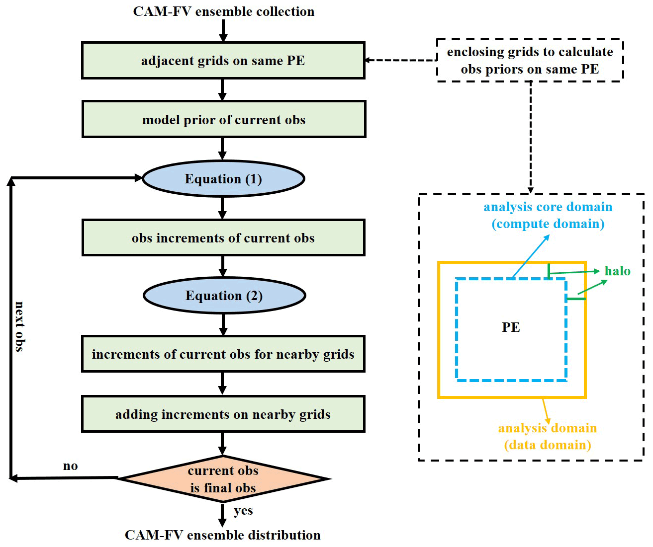
Figure 2Schematic of the implementation of the sequential EAKF algorithm with CAM-FV. The implementation is based on the two-step method of EAKF. The decomposition strategy allows adjacent grids to be divided into the same analysis domain (i.e., onto the same analysis PE). One analysis core domain (compute domain) and its halo constitute one analysis domain (data domain). When the observations at a given time are available, only the prior ensemble of a single observation is first computed. Then each observation is assimilated sequentially according to the two-step EAKF algorithm. The observational increments of an observation only regress on the nearby model states.
The ADA system with CAM-FV is realized using the two-step method of EAKF (Anderson, 2003; Zhang and Rosati, 2010) based on the online ensemble collection and distribution processes. As Fig. 1a shows, after the online ensemble collection, each PE obtains the ensemble vector of model states for an analysis domain. Then, the observational increment is calculated based on Eq. (1) on all PEs in parallel. It should be noted that one observation will be assimilated only if the ensemble of all state variables required for the forward operator calculation is available on the current PE. After the observational increments are obtained, they are projected onto the nearby model states to get the analysis increments via linear regression expressed by Eq. (2). Thus, the nearby model states can be updated by this observation via adding the analysis increments onto the background model states. Therefore, the model states used in the assimilation of the current observation have already been updated by all previous assimilated observations. This two-step assimilation process is repeated sequentially for the subsequent observations until all available observations of the current analysis step are processed. Finally, the analysis ensemble in the analysis core domains needs to be converted back to each member model space by online ensemble distribution to be ready for the next integration stage.
3.2 ADA with CAM-SE
3.2.1 Online ensemble collection and distribution with CAM-SE data structure
Unlike the regular latitude–longitude horizontal grid used in CAM-FV, CAM-SE uses a cubed-sphere grid in the horizontal direction (Dennis et al., 2012; Evans et al., 2013), which is no longer a logically rectangular grid. The direct effect of using such a grid on the form of data storage in the model space is that the model states are no longer represented as two-dimensional variables in the horizontal direction but are combined into one dimension. Taking the ne30np4 resolution of CAM-SE as an example, the two horizontal dimensions of the model variables in the geophysical space are represented by one dimension of length 48 602 in the array form. Moreover, due to the characteristics of the cubed-sphere grid, two adjacent grid points in the horizontal one-dimensional representation of the variable with CAM-SE may not represent the two grid points being adjacent in the geophysical space. Therefore, the parallel decomposition strategy of the analysis domain with CAM-FV is no longer applicable to CAM-SE because the adjacent model grid points in the geophysical space can no longer always be ensured to be divided and stored on the same PE.
In order to implement the online ensemble collection and distribution with CAM-SE, the model state variables are vectorized. When the model reaches the analysis time, the ensemble of model states is first obtained based on the collection function of MPI. This process is similar to that with CAM-FV, except that the collected state variables are all one dimension fewer than the same variables with CAM-FV. Then, all state variables of a single ensemble member are converted into a one-dimensional array. In principle, the arrangement of the model grid points in this array can be in an arbitrary order because the location information of each point will be recorded by a separate array. In this way, the ensemble of all model state variables will be represented by a two-dimensional array, where one dimension corresponds to the grid point sequence number, and the other represents the ensemble sequence number. Then, the parallel decomposition of the analysis domain is achieved by dividing the grid point dimension over all PEs. As a result, each PE obtains the information about the ensemble of a subsequence of model state variables. However, it should be emphasized that the grid points in this subsequence in principle can be arbitrarily distributed and are not required to be adjacent in the geophysical space. At this point, the data conversion from the model integration space based on the online ensemble collection to the analysis space with CAM-SE is completed. When the assimilation of all available observations at the current time is completed, the updated analysis ensemble obtained in the analysis space is converted back to the model space. This process is an inverse of the collection procedure and is implemented based on the MPI distribution function. Figure 1b shows an example of the parallel domain decomposition and online collection and distribution with a total of eight PEs and four ensemble members with CAM-SE.
3.2.2 Implementation of parallel EAKF algorithm with CAM-SE
The implementation of the ensemble filter with CAM-SE is also based on the two-step EAKF algorithm. Different from CAM-FV, the implementation needs to be adapted to the specific decomposition strategy of the analysis domains with CAM-SE. The differences are mainly in the computation of the observation prior ensemble and the regression of the observational increments. Figure 3 shows the schematic of the implementation of the parallel EAKF algorithm with CAM-SE.
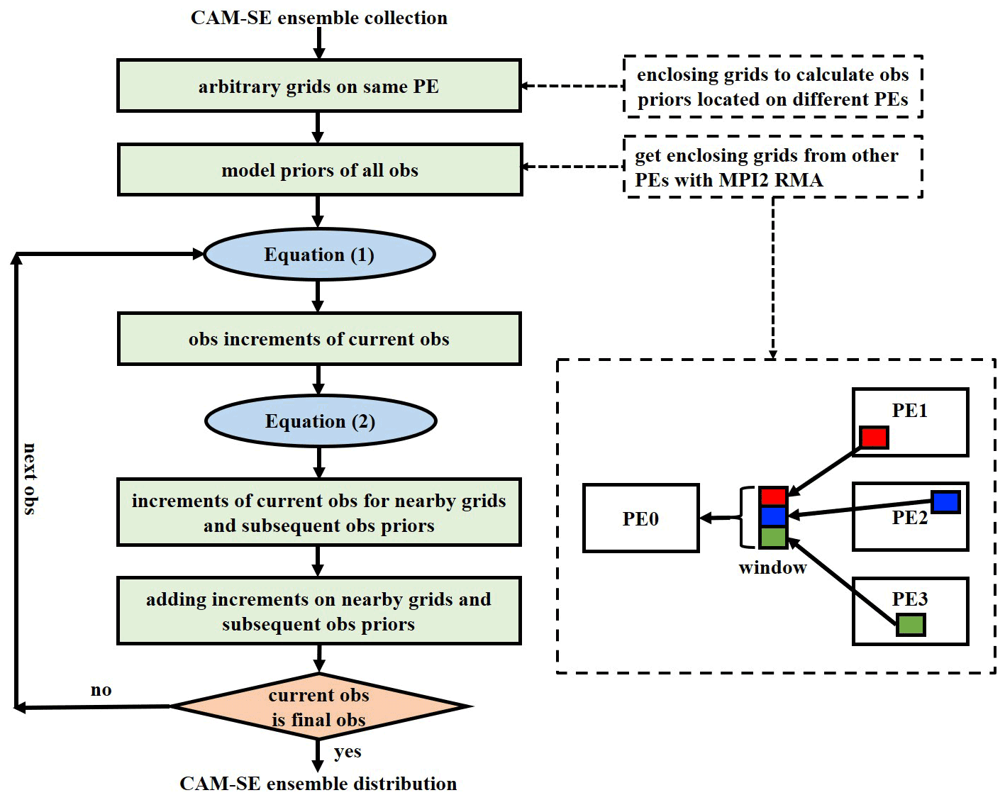
Figure 3Schematic of the implementation of the parallel EAKF algorithm with CAM-SE. The implementation is also based on the two-step method of EAKF. In CAM-SE, the grid points are decomposed onto the analysis PEs in an arbitrary way. Therefore, the computation of the forward observation operator may need to obtain values from other PEs, which is realized through the MPI2 RMA technique. The lower-right dashed rectangle illustrates an example of grabbing data from PEs 1–3 to PE0 via a virtual window of RMA. When the observations at a given time are available, the prior ensembles for all observations are computed. The observational increments of an observation regress not only on the nearby model states, but also on the subsequent observation prior ensembles.
The computation of the observation prior ensemble with CAM-SE uses the same method as DART (Anderson et al., 2009), which is implemented based on the remote memory access (RMA) technique of MPI2 (Gropp et al., 1999). Because the grid points are divided onto different PEs in an arbitrary way, the four grid points enclosing one observation for interpolation may be located on different PEs from the owner PE of the observation. In the best case, all four enclosing points are located on the same PE as the owner PE, while in the worst case, all four enclosing points are located on four different PEs. Therefore, it needs to obtain the model background from the memories of other PEs (i.e., remote memories) for computing the observation priors. In order to fulfill this requirement, the RMA technique of MPI2 is used, which allows one PE to asynchronously read or write the memories of other PEs through a virtual window. Thus, regardless of which PEs the four enclosing points of the observation are located on, the prior ensemble for this observation can be obtained with aids of the RMA technique. Then the observational increment ensemble can be calculated based on Eq. (1).
The regression of the observational increments with CAM-SE is based on a parallel implementation of the EAKF algorithm (Anderson and Collins, 2007). With CAM-FV, the observational increments are mapped onto the nearby model grids via linear regression to obtain the analysis increments of the nearby model states. With CAM-SE, the calculation of the observation priors requires access to the remote memories through RMA, which is more complex and computationally expensive than the direct access to the local memory with CAM-FV. To optimize the filtering algorithm with CAM-SE, the computation of the forward observation operator is implemented based on a parallel algorithm of Anderson and Collins (2007). This algorithm is suitable for the parallel implementation of the EAKF algorithm. It splits the traditional forward observation operator computation, executed once for each observation, into a one-time calculation for all observations and an update of the nearby subsequent observation priors which have not been assimilated. Therefore, with CAM-SE, the forward operator computation is executed only once for each assimilation step. In this parallel implementation, the prior ensembles are first computed for all observations using the model background that has not been affected by any observation. Then, when an observation comes in, its observational increments update not only the nearby model states as in CAM-FV, but also the prior ensembles of all nearby observations that have not been assimilated (i.e., the subsequent observation priors). This parallel algorithm has been shown to produce identical results to the traditional sequential algorithm. More details of this parallel implementation can be found in Anderson and Collins (2007).
3.3 ODA with POP
The online collection and distribution processes with POP are similar to those with CAM-FV (Fig. 1a). Although the horizontal grid used in POP is different from the regular latitude–longitude grid in CAM-FV, they both belong to the logically rectangular grid. More specifically, the horizontal dimensions of model variables can be represented by latitude and longitude. Therefore, similar parallel domain decomposition strategy based on the geophysical space to that with CAM-FV is used with POP to obtain the analysis domain. With CAM-FV, the decomposition of the analysis domains is based on the global horizontal field, while with POP, the analysis domain decomposition is further optimized via a so-called local secondary decomposition on the model integration domain. In this local secondary decomposition strategy, the same model integration domains of all ensemble members are directly decomposed onto the PEs responsible for the integration calculation of these integration domains of all ensemble members. Taking Fig. 1a as an example, the southwest (i.e., lower-left) integration domains of four ensemble members are decomposed onto PEs 0, 4, 8, and 12 to obtain the analysis domains. Because the collection of the entire global field of model states can be avoided (replaced by the collection of a subset of the global field), this local secondary decomposition strategy with POP reduces the hard limit on the PE storage capability. However, it should be pointed out that one disadvantage of this decomposition method is that the halo width in the analysis domain cannot exceed that of the integration domain. The implementation of the sequential EAKF algorithm with POP is the same as that of CAM-FV (see Fig. 2); thus it is not repeated here.
3.4 The online CESM-ECDA system
When the DA systems in CAM and POP have each been developed, the ocean–atmosphere CESM-ECDA system can be constructed. Figure 1c shows the implementation framework of the CESM-ECDA system. In one assimilation cycle, the execution of the CESM-ECDA system can be described as follows. The CESM model reads in the initial condition ensemble to start the forward integration of the model ensemble. When the model integration reaches the observation time, the model ensemble integration is suspended. Then the forecast fields of CAM and/or POP are obtained as the background fields of the assimilation by the ADA and/or ODA components through the online ensemble collection, then the two-step update of EAKF is used for the sequential assimilation of the observations in each component. After the assimilation process has been completed, the analysis fields obtained by ADA and/or ODA are transformed back to corresponding model spaces through the online ensemble distribution. Then the analysis ensemble updated by the observations is used as the initial states for the model ensemble to continue the integration in the next forecast stage. It should be noted that the ADA and ODA components can be executed using the same or different frequencies. Generally, the ODA interval is longer than that of ADA to account for the different characteristic timescales between the ocean and the atmosphere because the background fields used in ADA and ODA come from the atmosphere and ocean components of the coupled CESM, and the dynamic coupling between the atmosphere and ocean components is performed through the interface fluxes in the model forecast stage. The observed information in the atmosphere and ocean can be exchanged with each other, so that the coupled state estimation obtained by the CESM-ECDA is more self-consistent and balanced. In addition, because the coupled covariance between the atmosphere and the ocean is not used in the current CESM-ECDA system, the observation in one component is not allowed to directly update the model state in the other component in the assimilation stage, which makes it a weakly coupled DA (WCDA) system.
4.1 ADA with CAM-FV
The assimilation of Ps observations by ADA with CAM-FV significantly improves the atmospheric surface variables. Figure 4a–e show the time series of RMSEs of five atmospheric surface variables, and Table 2 shows the global averaged RMSEs. To focus on the impact of assimilation after the system reaches equilibrium, the globally averaged RMSEs of atmospheric variables and fluxes are calculated with the experiment output data of the first month excluded in this paper. By assimilating Ps observations, not only the surface pressure, but also other atmospheric variables are significantly improved. Compared with the ctl, the RMSEs of surface variables are clearly and rapidly reduced by assimilating Ps observations. The global averaged RMSE of Ps is reduced from 6.68 to 4.05 hPa, nearly improved by 40 %. The RMSEs of the other four variables are reduced by about 15 %–25 %.
Table 2Globally averaged RMSEs of surface pressure Ps, surface temperature Ts, surface specific humidity Qs, surface zonal wind Us, and surface meridional wind Vs from ctl and ada_fv. The RMSEs are calculated with the data of the first month excluded.
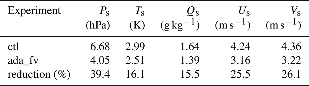
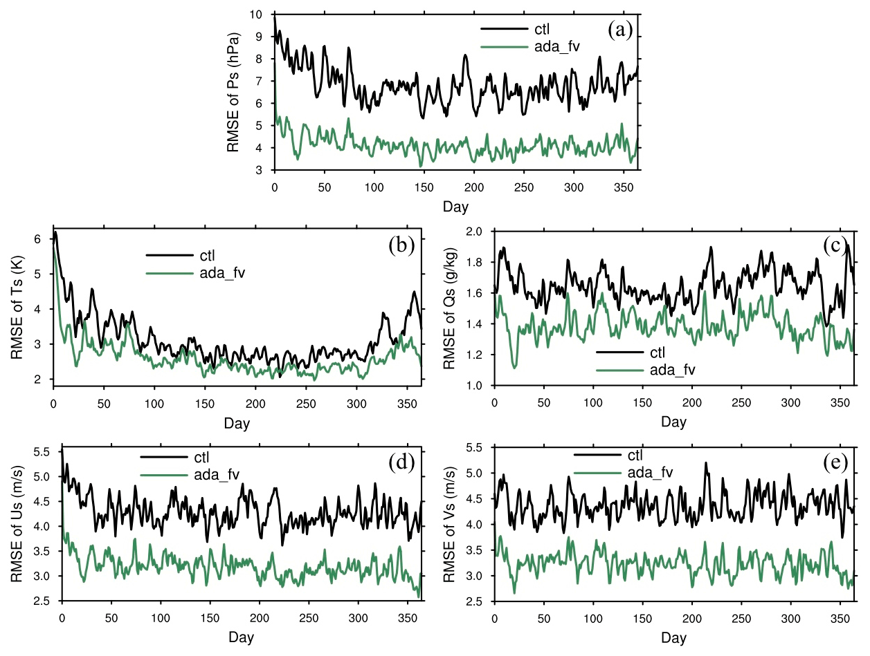
Figure 4Time series of RMSEs of (a) surface pressure Ps, (b) surface temperature Ts, (c) surface specific humidity Qs, (d) surface zonal wind Us, and (e) surface meridional wind Vs from ctl and ada_fv.
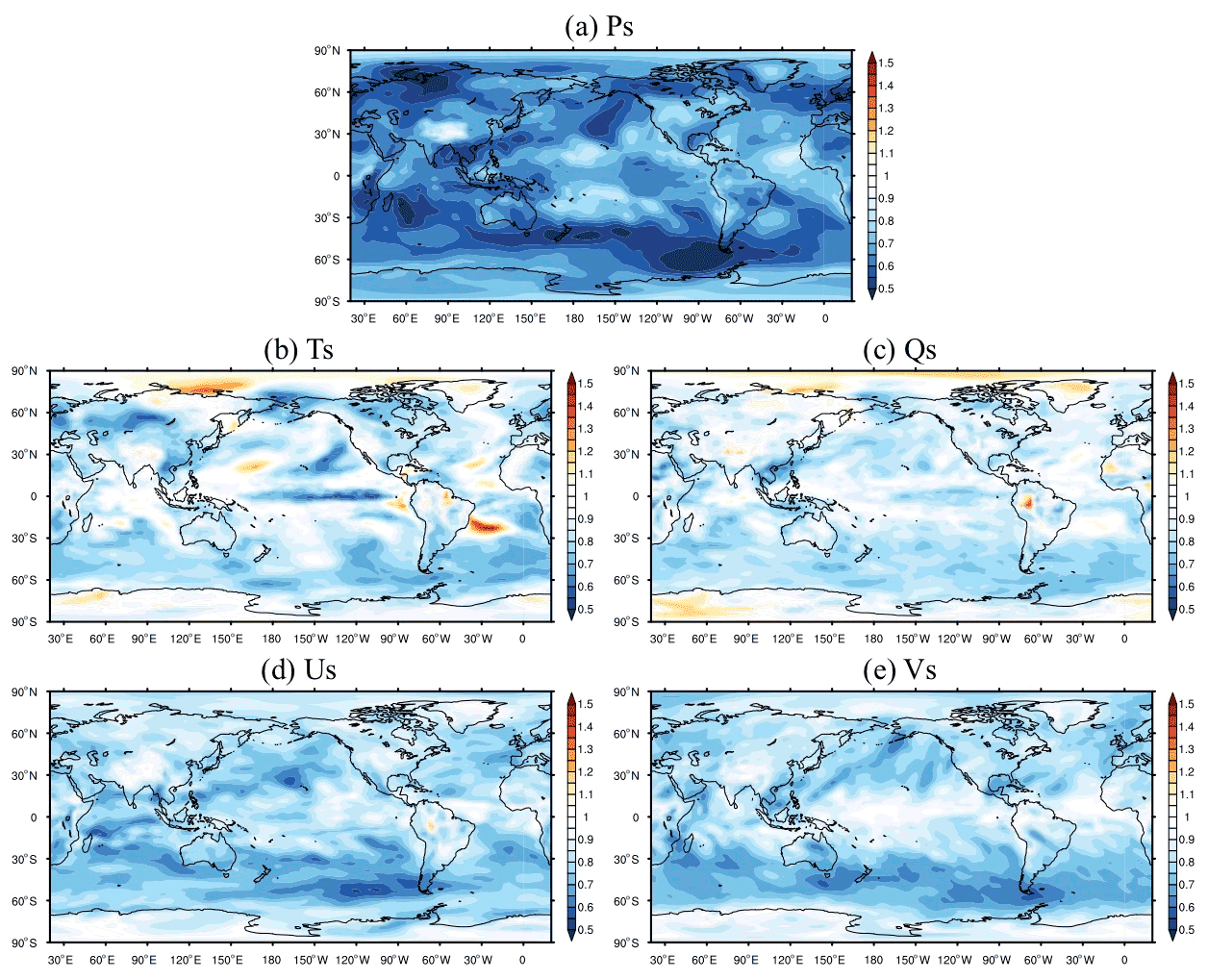
Figure 5The distribution of the RMSE ratio (ada_fv/ctl) of (a) surface pressure Ps, (b) surface temperature Ts, (c) surface specific humidity Qs, (d) surface zonal wind Us, and (e) surface meridional wind Vs. The RMSE ratios are calculated with the data of the first month excluded.
Figure 5a–e show the distribution of the ada_fv-to-ctl (hereafter ada_fv/ctl) RMSE ratio of the five atmospheric surface variables. Compared to ctl, which does not assimilate observation, the assimilation of Ps in ada_fv can significantly reduce the RMSE of Ps all over the globe. The RMSEs of Us and Vs are also reduced throughout the globe in ada_fv. Though the RMSEs of Ts and Qs are increased in some regions in ada_fv, the assimilation of Ps observations can improve the analysis accuracy over most regions. In addition, the improvements are mostly located at the midlatitudes on both hemispheres, especially in the Southern Hemisphere. Ps is a two-dimensional variable, but it contains abundant three-dimensional information of the atmosphere. Therefore, the solo assimilation of Ps observations not only significantly corrects the model Ps field, but also improves other atmospheric variables. It should be pointed out that U, V, T, and Q are not used as direct assimilating variables but are adjusted through the dynamic process and physical process of the model after assimilating Ps. And the errors of these variables are also significantly reduced, which shows that the assimilation effect of the system in the model is reasonable.
4.2 ADA with CAM-SE
The atmospheric surface variables by assimilating the Ps observations within CAM-SE are also significantly improved. Figure 6a–e show the time series of RMSEs of five atmospheric surface variables, and Table 3 shows the global averaged RMSEs. The calculation of the global averaged RMSEs also excludes the output data of the first month. Generally speaking, the assimilation effects of Ps observations with CAM-FV and CAM-SE are similar. The ADA system with CAM-SE can also significantly improve the atmospheric variables over the ctl experiment; even only the Ps observations are assimilated. Furthermore, the amplitude of the RMSE reduction with CAM-SE tends to be smaller than that with CAM-FV, especially for Ps, Us, and Vs (Table 2 vs. Table 3). For example, compared with the ctl experiment, ada_fv reduces the RMSEs of Ps, Us, and Vs by up to 39.4 %, 25.5 %, and 26.1 %, respectively, while the corresponding RMSE reductions in ada_se are 29.4 %, 20.1 %, and 17.0 %, respectively. In addition, the horizontal distribution of RMSE in SE (not shown here) is similar to that in FV.
Table 3Globally averaged RMSEs of surface pressure Ps, surface temperature Ts, surface specific humidity Qs, surface zonal wind Us, and surface meridional wind Vs from ctl and ada_se. The RMSEs are calculated with the data of the first month excluded.
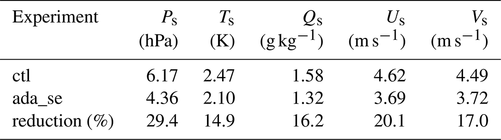
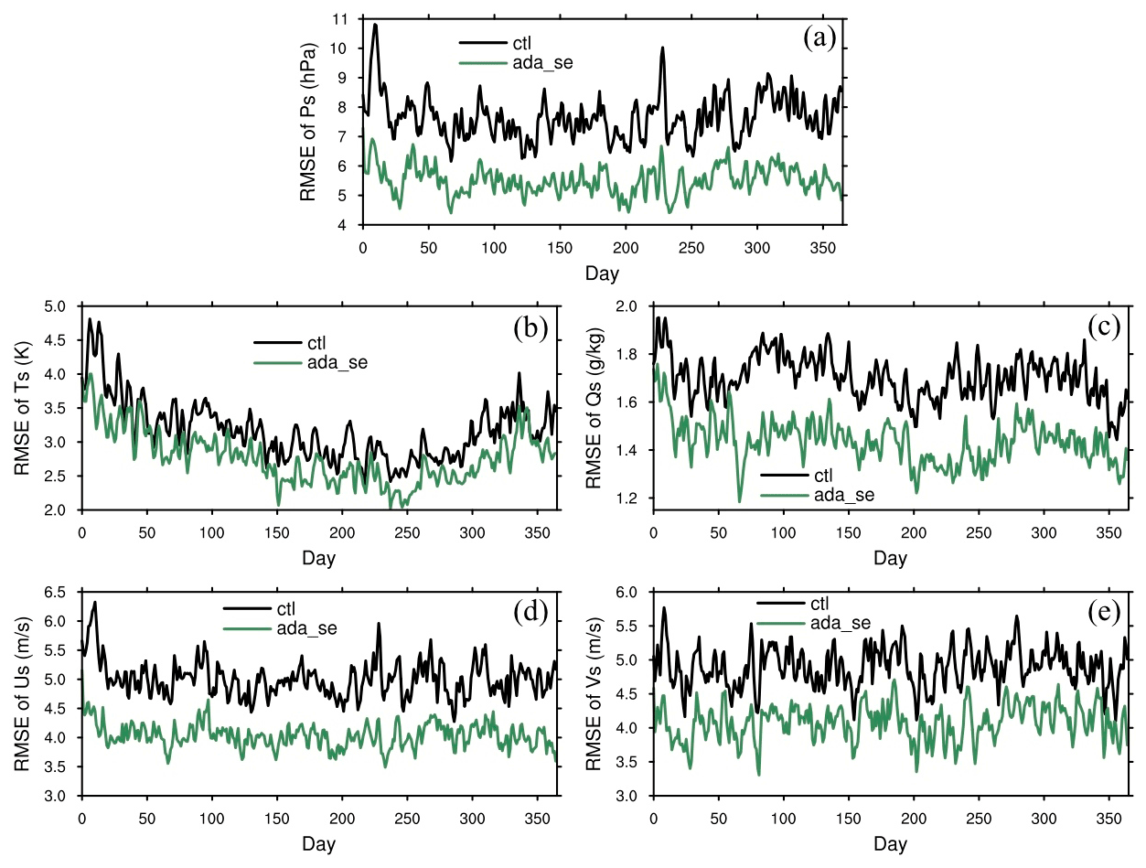
Figure 6Time series of RMSEs of (a) surface pressure Ps, (b) surface temperature Ts, (c) surface specific humidity Qs, (d) surface zonal wind Us, and (e) surface meridional wind Vs from ctl and ada_se.
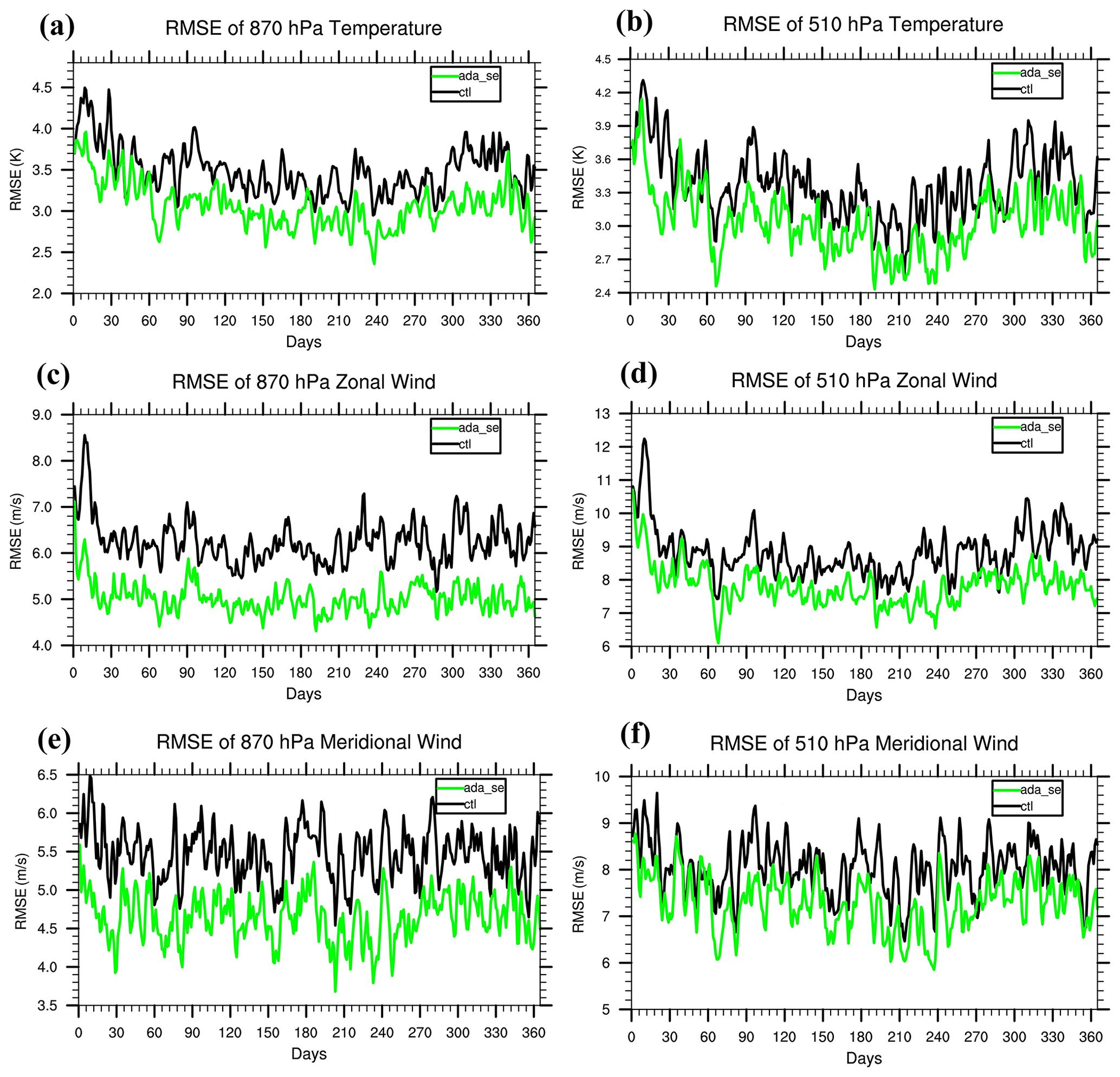
Figure 7Time series of RMSEs of (a) 870 hPa temperature, (b) 510 hPa temperature, (c) 870 hPa zonal wind, (d) 510 hPa zonal wind, (e) 870 hPa meridional wind, and (f) 510 hPa meridional wind from ctl (black lines) and ada_se (green lines).
Figure 7a–f show the time series of RMSEs of upper-layer atmospheric variables, temperature and winds at 870 and 510 hPa being examples. The RMSEs of all these three variabilities in ada_se are also smaller than those in ctl experiment in the high-level atmosphere. At the 870 hPa level, the RMSEs of temperature, zonal wind, and meridional wind from ctl are 3.43 K, 6.18 m s−1, and 5.45 m s−1. After only assimilating the surface pressure, these RMSEs are decreased to 3.02 K, 4.99 m s−1, and 4.64 m s−1 respectively. At the 510 hPa level, the RMSEs from ctl are 3.32 K, 8.72 m s−1, and 8.01 m s−1, while the RMSEs from ada_se are 3.00 K, 7.72 m s−1, and 7.24 m s−1 respectively. The model errors of other atmospheric variables are also reduced, which will not be displayed one by one here. It is worth mentioning that the reduction rate of RMSEs for the variables in the upper layers is much smaller than that in the surface. This might suggest that the simultaneous increments of three-dimensional winds, temperature, and moisture are very important for representing the atmosphere state in the whole troposphere (Yang et al., 2021). When there are enough computing resources in the future, we will consider increasing the ensemble size to assimilate three-dimensional atmospheric variables to further improve results.
One aspect of surface pressure data assimilation shown in 20CR is that it could have very similar weather-to-climate-scale variability in the troposphere to other traditional atmosphere reanalyses which use all available observations. Figure 8a–b show the distribution of the anomaly correlation coefficient (ACC) between ctl (ada_se) and truth at 500 hPa geopotential height. The ACC between ctl and truth is about 0.6–0.9 in Eurasian continent and about 0.5–0.7 in North America (Fig. 8a). In North Pacific and North Atlantic, the maximum ACC of ctl and truth is about 0.8, and the minimum is about 0.3. In the Southern Hemisphere, the ACC of ctl and truth is much smaller than that in the Northern Hemisphere. For example, south of 30∘ S, the ACC of ctl and truth is below 0.4 in the Southern Ocean. It may be related to the large simulated interannual variability of CESM in the Southern Hemisphere since we use the results of CESM in another year as truth. Globally, the areas with the smallest ACC are the equatorial Pacific and the equatorial Indian Ocean; ctl and truth are basically negatively correlated, which may be related to the high-frequency motions in the equatorial region. The ACC of ada_se and truth increases significantly after assimilation (Fig. 8b). The maximum value of ACC in the Eurasian continent can reach 0.9–1.0, and the ACC also increases significantly in North America, Southern Ocean, equatorial ocean, and other regions. Figure 9a shows the time series of 500 hPa geopotential height RMSE. Compared with ctl, the RMSE of ada_se significantly reduces. It can be considered that the weather variability in the middle troposphere is retrieved by the surface pressure data assimilation.
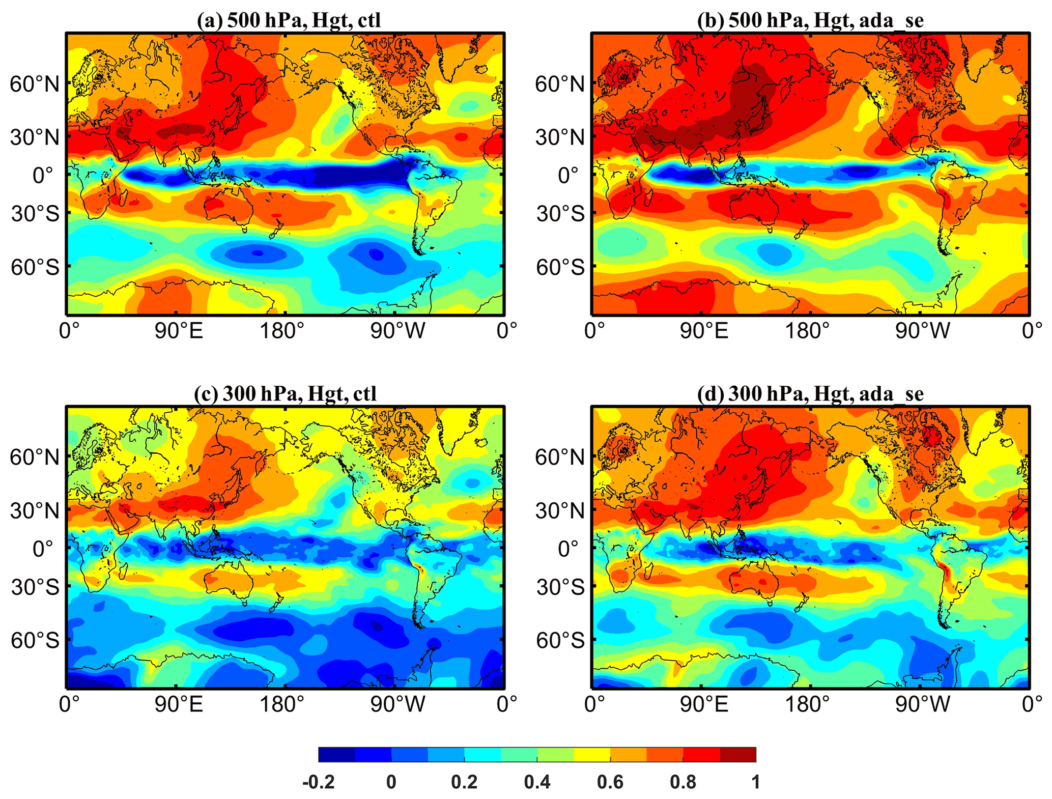
Figure 8Map of the local anomaly correlation between four-times-daily anomalies of 500 hPa (a, b) and 300 hPa (c, d) geopotential (a, c) between ctl and truth and (b, d) between ada_se and truth. Anomalies are computed separately for each dataset with respect to the mean annual cycle of the period shown.
Figure 8c–d show the distribution of ACC between ctl (ada_se) and truth at 300 hPa geopotential height. The ACC between ctl and truth in the Northern Hemisphere is higher than the Southern Hemisphere, which is similar to 500 hPa. The Northern Hemisphere is basically above 0.5, and the Southern Hemisphere is below 0.4, except for areas around 30∘ S. The ACC in the equatorial region is also relatively low, which is similar to 500 hPa. After assimilating the surface pressure, the result of geopotential height at 300 hPa is significantly improved. The ACC increases all over the world. For example, the ACC is about 0.7–0.9 in the Northern Hemisphere continent and about 0.2–0.5 in the Southern Ocean. Figure 9b shows the time series of 300 hPa geopotential height RMSE. Compared with ctl, the RMSE of ada_se significantly reduces, which is similar to 500 hPa. It can be considered evidence that the weather variability in the upper troposphere is adjusted through the dynamic process and physical process of the model after assimilating surface pressure.
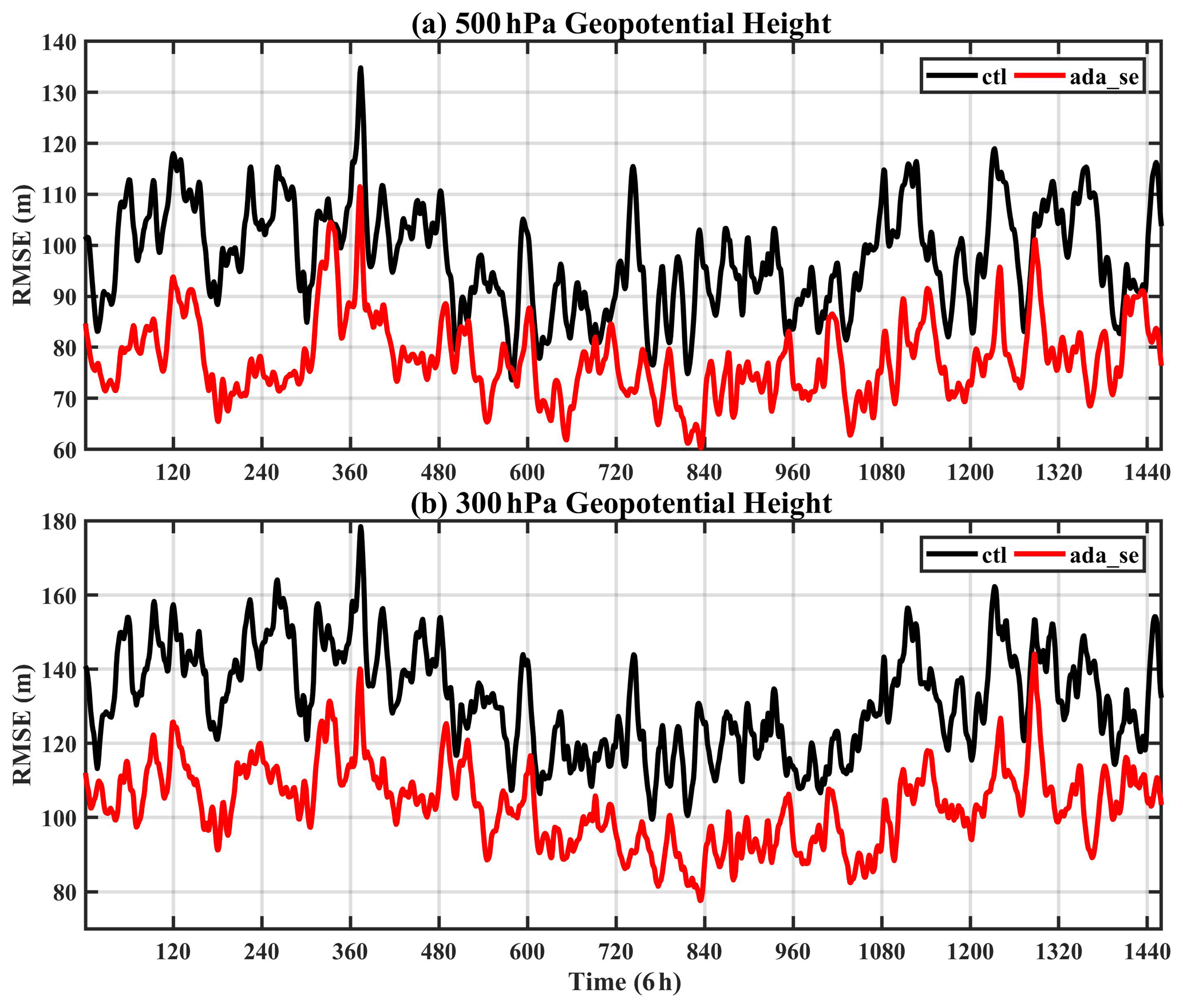
Figure 9Time series of RMSEs of (a) 500 hPa geopotential and (b) 300 hPa geopotential from ctl (black lines) and ada_se (red lines).
4.3 ODA
4.3.1 Assimilation of SST
The assimilation of SST observations by the ODA system with POP significantly improves the accuracy of the ocean states. Figure 10a–b show the time series of RMSE of SST from ctl and oda_sst and the distribution of the oda_sst-to-ctl (hereafter oda_sst ctl) RMSE ratio of SST. To focus on the impact of assimilation after the ocean system reaches equilibrium, the global averaged RMSE and the RMSE ratio of the oceanic variables are computed with the output data in which the first 3 months were excluded in this paper. Compared with the ctl experiment, the RMSE of SST in oda_sst significantly and quickly reduces at the beginning of the experiment and then gradually decreases further and stays stable. The SST RMSE in oda_sst reduces from 0.58 to 0.13 K. The distribution of the RMSE ratio (oda_sst ctl) shows that the oda_sst experiment can improve the quality of SST over almost the entire globe, except in the high-latitude regions of the Northern Hemisphere. In addition, the distribution of the improvement in oda_sst is relatively uniform compared with that in the ADA experiments discussed above. By assimilating SST, the RMSE of SST is significantly reduced, which is consistent with previous studies such as CFSR (Saha et al., 2010).

Figure 10(a) Time series of RMSE of SST from ctl and oda_sst and (b) the distribution of the RMSE ratio (oda_sst ctl) of SST. The RMSE ratio is calculated with the data of the first 3 months excluded.
4.3.2 Assimilation of in situ ocean profiles
The design of the assimilation of in situ ocean profile temperature and salinity observations with POP is similar to the EAKF algorithm of CM2.1-ECDA (Zhang et al., 2007), since the locations of the real profile observations are changing over time, and they are not coincident with the model grid points. The first step of profile assimilation is to get the model values at the positions of profiles by interpolating and then calculating the observational increment. When calculating the observational increment, eight-point interpolation is used; that is, both the upper and lower four points are used for the interpolation to obtain the model value at the observational point. The second step is to project the observational increment onto the surrounding model grid points. In the vertical direction, each profile affects one layer above and one layer below, with a total of two model layers. The same as the previous study (Zhang et al., 2007), the impact of temperature on salinity and the impact of salinity on temperature are both activated. In accordance with the SST assimilation, the frequency of profile observation assimilation is also 1 d. The distributions of the profile observations are shown in Fig. 11a–d.
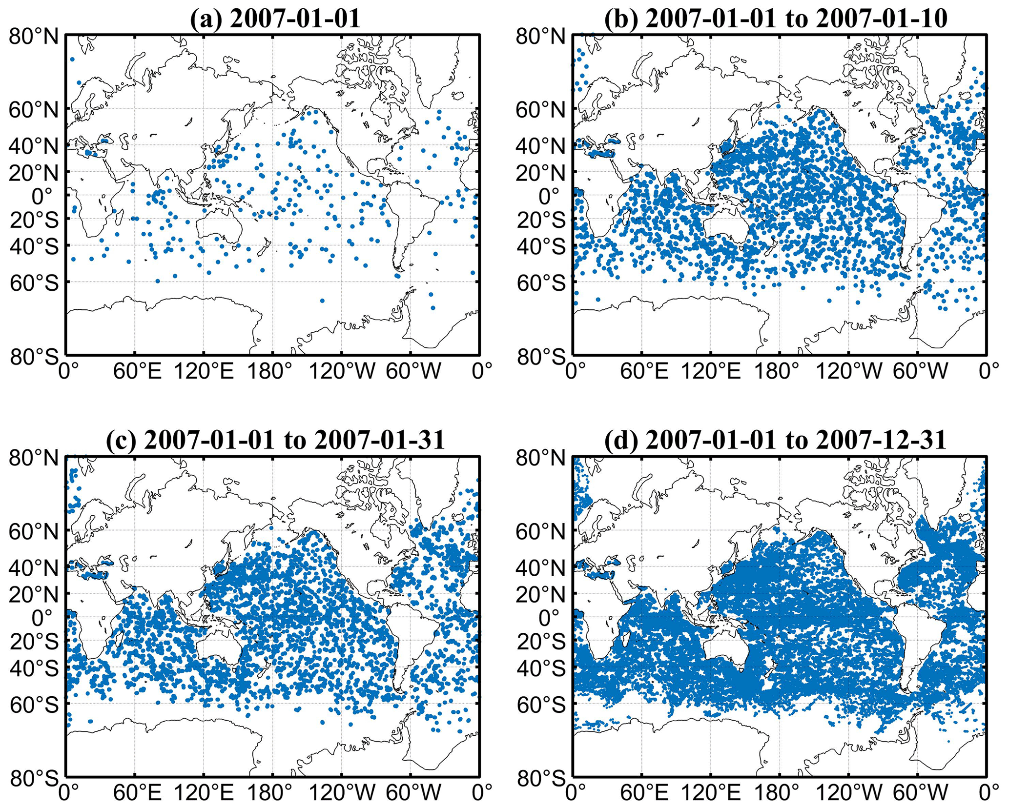
Figure 11Argo locations on (a) 1 January 2007, (b) 1 to 10 January 2007, (c) 1 to 31 January 2007, and (d) 1 January to 31 December 2007.
The addition of ocean profile observations to the ODA system further significantly improves the ocean state estimates over the control run. Figure 12a–d show the time series of RMSEs of ocean temperature and salinity vertically averaged from 0–500 and 500–2000 m from the ctl and oda experiments. And Table 4 shows the global averaged RMSEs of these four variables, with the data of the last 6 months. Compared with the ctl experiment, the RMSEs of temperature and salinity are both significantly reduced. Assimilation of temperature and salinity profile observations rapidly reduces the RMSE compared to ctl at the beginning of the experiments in 0–500 m. Compared with the salinity, the RMSE of temperature decreases more rapidly to a stable level (approximately 3–4 months for the temperature vs. 7–8 months for the salinity). In addition, at the same depth range, the improvement of the temperature tends to be larger than the salinity, with the RMSE reduction of 25.0 % (9.9 %) and 7.1 % (1.2 %) for 0–500 m (500–2000 m) temperature and salinity, respectively. And for the same variable, the reduction of RMSE in the shallower ocean is larger than the deeper ocean (Table 4), which may be caused by the slower variability of the deeper ocean.
Table 4Globally averaged RMSEs of ocean temperature and salinity vertically averaged between the surface and 500 m and between 500 and 2000 m from ctl and oda with the data of the last 6 months.
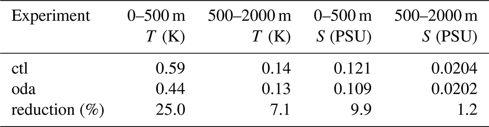
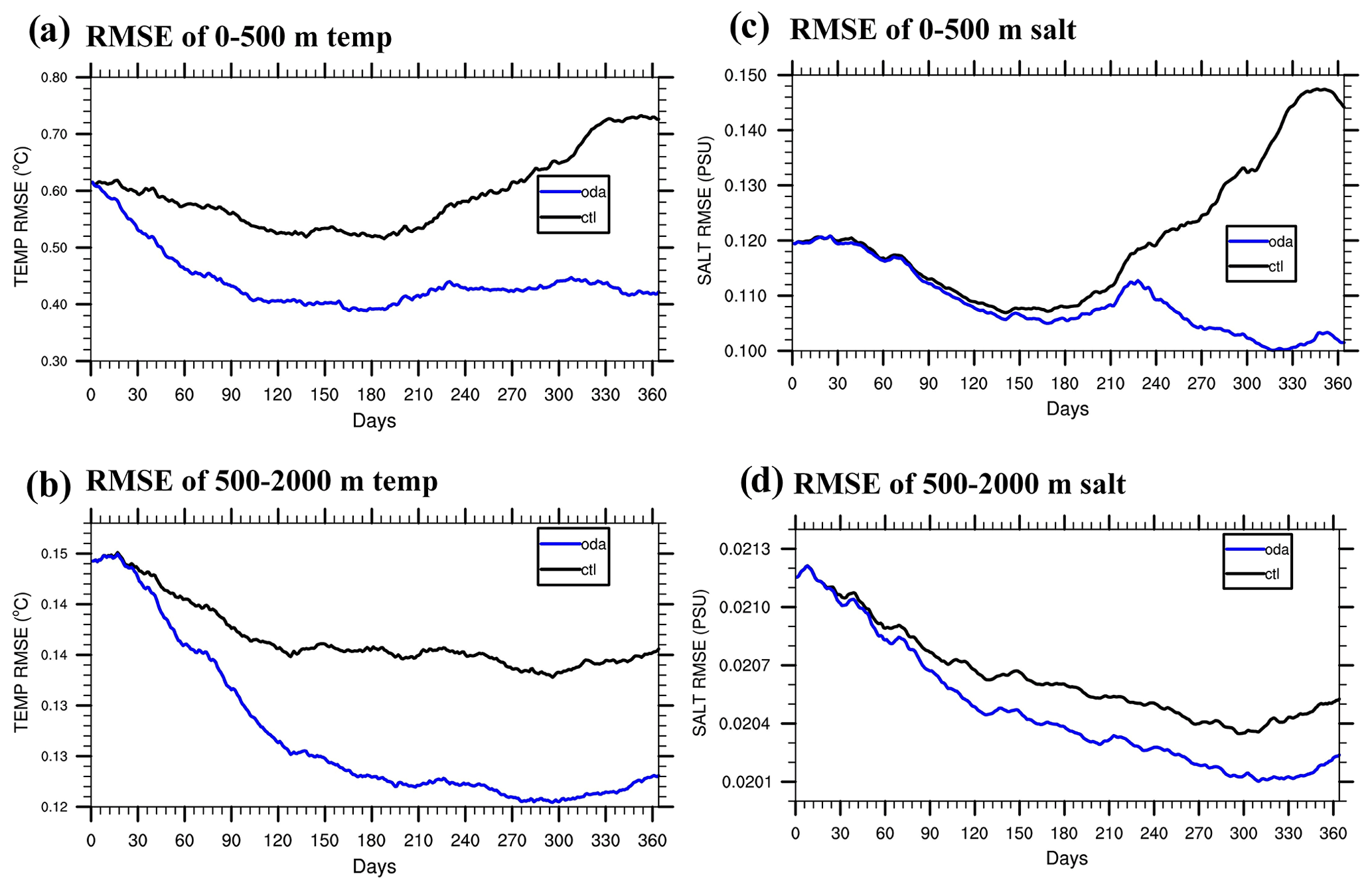
Figure 12Time series of RMSEs of (a) 0–500 m and (b) 500–2000 m ocean temperature and (c) 0–500 m and (d) 500–2000 m ocean salinity from ctl (black line) and oda (blue line).
Compared with ctl, oda greatly improves the ocean temperature and salinity estimates, especially in the shallow ocean (0–500 m). The RMSEs of ocean temperature and salinity are clearly reduced in most regions of the globe between the surface and 500 m depth, in addition to the coast of Africa and the high-latitude areas of the North Pacific. The largely improved regions are mostly located in the low-latitude to midlatitude regions, especially in the Pacific and Indian oceans. In the deeper ocean (500–2000 m), the improvement of temperature and salinity is less significant than in the upper ocean, showing a small RMSE reduction from ctl compared to the upper ocean. Overall, the improvement of salinity is smaller than temperature. This method of improving ocean model state estimate by assimilating temperature and salinity profiles has also been applied in previous studies, such as Zhang et al. (2007) and Carton et al. (2018). The conclusion in this work is basically consistent with them.
4.4 CDA
After the ADA and ODA components have been implemented based on CAM and POP, respectively, the CESM-ECDA system is also constructed. Because the ocean–atmosphere coupled error covariance is not used in the CESM-ECDA system, the observation in one component system (such as the atmosphere) cannot directly affect the model state in another component (such as the ocean) in the analysis stage. Therefore, the CESM-ECDA system is implemented in the WCDA style. In the current version of the CESM-ECDA system, the ADA component is capable of assimilating the atmospheric observations of the two-dimensional surface pressure, the three-dimensional temperature, wind components, and humidity; and the ODA component can assimilate the oceanic observations of the two-dimensional SST and the three-dimensional in situ profiles of temperature and salinity. In addition, the localization, covariance inflation, and incremental analysis update (IAU; Bloom et al., 1996) schemes are also included. More specifically, the localization schemes include the variable localization, horizontal localization, and vertical localization based on the widely used filter from Gaspari and Cohn (1999), and the covariance inflation is applied with both the classic scheme from Anderson and Anderson (1999) and the relaxation-to-prior scheme (Zhang et al., 2004).
4.4.1 Impact of CDA on atmosphere state estimation
The CESM-ECDA system can improve the quality of the atmosphere state estimation over the single ADA experiment. When the assimilation of Ps observations in the atmosphere and SST observations in the ocean are both activated, the CDA system operates in a WCDA style (i.e., the cda experiment). Compared with the single ADA experiment, the cda experiment can be used to evaluate the assimilation performance of the CESM-ECDA system in the atmosphere. Figure 13a–e show the time series of RMSEs of five atmospheric surface variables. When the Ps and SST observations are both assimilated, the cda experiment can further reduce the RMSEs of the atmospheric variables in comparison with the ada_fv experiment, which only assimilates the Ps observations into the atmosphere.
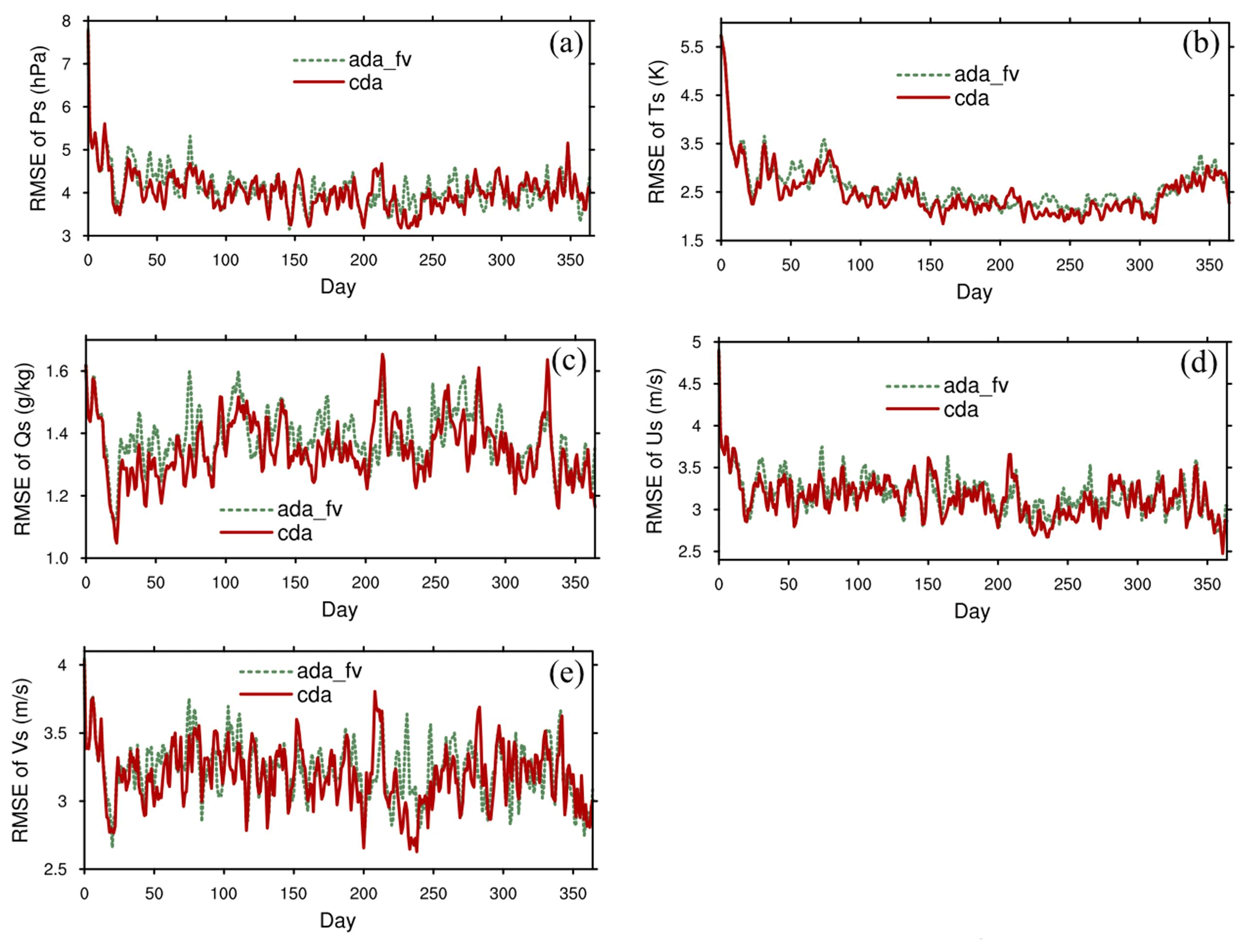
Figure 13Time series of RMSEs of (a) surface pressure Ps, (b) surface temperature Ts, (c) surface specific humidity Qs, (d) surface zonal wind Us, and (e) surface meridional wind Vs from ada_fv and cda.
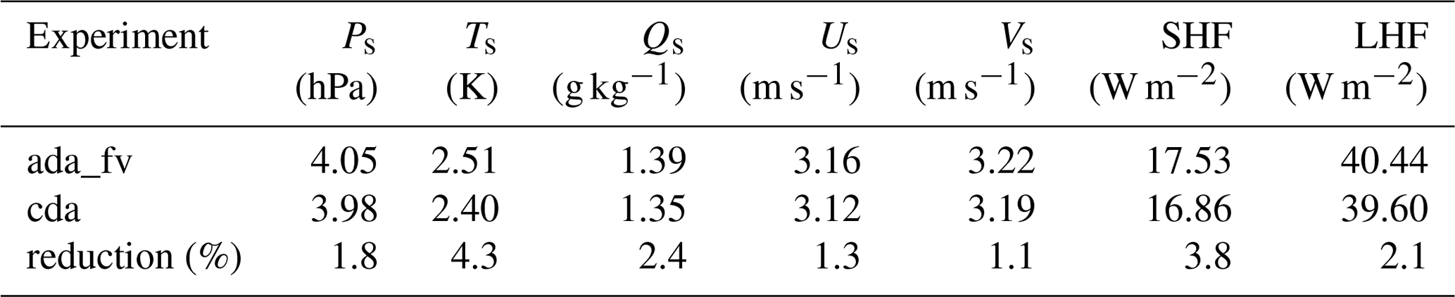
Table 5 lists the global averaged RMSEs of these five variables and three important air–sea interface fluxes with the data. Although the cda experiment can improve all the atmospheric surface variables considered here over ada_fv, the error reductions are small (approximately 1 %–2 %, and the Ts is 4.3 %). This may be caused by the strong correlation between the ocean temperature and atmosphere temperature near the air–sea interface, while the correlation between SST and other atmospheric surface variables is weak. Compared with ada_fv, the cda experiment further includes the assimilation of SST observations into the ocean component. Therefore, the model SST state is well constrained by the SST observations. The improved SST in cda can further benefit the overlying atmosphere through the ocean–atmosphere dynamic coupling. Although all atmospheric states should be improved by the better lower boundary conditions provided by the ocean, only those strongly correlated with the SST more significantly benefit from the improved SST.
Table 5Globally averaged RMSEs of surface pressure Ps, surface temperature Ts, surface specific humidity Qs, surface zonal wind Us, surface meridional wind Vs, sensible heat flux SHF, and latent heat flux LHF from ada_fv and cda. The RMSEs are calculated with the data of the first month excluded.
The cda experiment shows a mixed distribution of decreased and increased RMSE and a global averaged weak improvement for Ps, Qs, Us, and Vs. The regions of significant improvement are mostly located in the tropical eastern Indian Ocean and the tropical to subtropical Atlantic, which may indicate the more significant positive impact of the coupling between SST and air–sea fluxes. It should be noted here that the cda experiment can significantly improve the Ts state over almost the entire ocean areas, especially in the tropical Indian Ocean, the tropical to subtropical Atlantic, and the midlatitude Pacific.
The improvement of CESM-ECDA over single ADA experiment can also be reflected in the air–sea interface fluxes. Figure 14a–d show the time series and ratio (cda ada_fv) distribution of RMSEs of SHF and LHF. These fluxes can also be improved by the further assimilation of the SST observations into the ocean in the cda experiment. Compared with ada_fv, cda further reduces the RMSEs of SHF and LHF by 3.8 % and 2.1 % (Table 5), respectively. These two fluxes share significant improved regions with above variables, such as the tropical Indian Ocean and the tropical to subtropical Atlantic. The assimilation of SST observations in cda improves the air–sea coupling processes in these regions, leading to corrected interface fluxes there. Then the improved interface fluxes further transmit the correcting information to the overlying atmosphere.
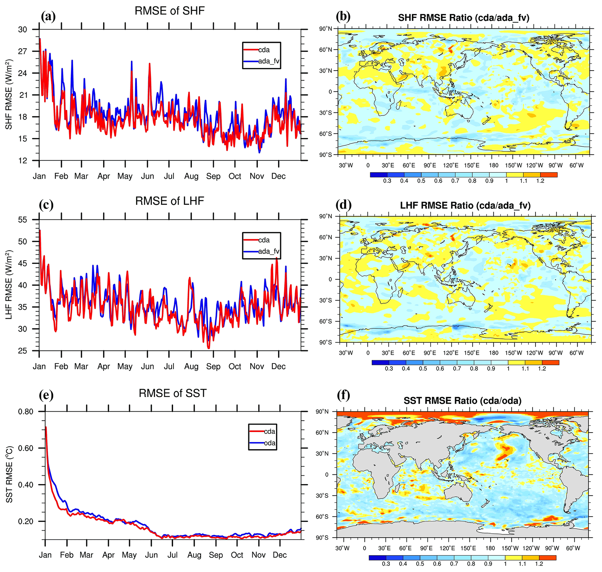
Figure 14Time series of RMSEs of (a) sensible heat flux (SHF), (c) latent heat flux (LHF) from ada_fv and cda, and (e) SST from oda_sst and cda and distribution of the RMSE ratio of (b) SHF (cda ada_fv), (d) LHF (cda ada_fv), and (f) SST(cda/oda). The RMSE ratios are calculated with the data of the first month excluded.
4.4.2 Impact of CDA on ocean state estimation
The CESM-ECDA system can obtain improved ocean states over the single ODA experiment. Figure 14e–f show the time series and distribution of the SST RMSE from the oda and cda experiments. Compared with oda which only assimilates the SST and profiles observations, cda further assimilates the Ps observations into the atmosphere component. Therefore, the comparison between oda and cda can be used to evaluate the impact of the CESM-ECDA system on the ocean state estimation. Assimilation of SST observations alone in the oda experiment has already largely reduced the SST RMSE in comparison with the ctl experiment, while cda can further reduce the SST RMSE by up to 10.4 % (from 0.134 to 0.120 K, with the data of the first 3 months excluded from the computation). The RMSE of SST can be significantly reduced in most regions except for the Arctic Ocean by further assimilating the Ps observations into the atmosphere. The SST RMSE in cda decreases about 10 %–20 % compared to oda. When Ps observations are assimilated into the atmosphere, the atmospheric states are better constrained, which provides an improved upper-boundary condition for the ocean.
4.5 Computational efficiency of online vs. offline CDA
The data assimilation can be implemented by either an offline or an online mode. In offline mode, data assimilation and model integration are independently performed in two programs, for which at each assimilation time the model integration needs to stop and write (read) model states on (from) local disks for assimilation (next model integration). In online mode, data assimilation and model integration are performed in one program, in which the model integration and assimilation are linked by memory management. Both online and offline assimilation modes share model integration and assimilation consumptions, but the offline mode needs additional I/O and initialization consumptions at each assimilation step. So, their difference of CPU (central processing unit) time mainly depends on the process of initialization and I/O, as well as the assimilation frequency.
If at an assimilation interval, the model initialization and I/O time is A, model integration time is B, analysis time is C, and the total CPU time in offline and online assimilation is respectively and for n assimilation steps. So, the ratio between online time and offline time can be expressed as
As n is large enough, . The CPU time saved by online assimilation mainly depends on the proportion of (B+C) and A. For example, if , ; if , . By the way, here we only discuss the difference of CPU times in offline and online assimilation modes. However, depending on the performance of the HPC (high-performance computing) system, the I/O process wall clock time may be much longer than the CPU time.
Table 6 presents the comparison of CPU time in offline cda experiments and online cda experiments. We use the resolution of ne30_g16 and the component setting of B1850CN for system evaluation. The assimilation frequency is daily in ocean and 6-hourly in atmosphere. The number of observations is the same every day. The ensemble size is set to 12, and each member uses 32 PEs (32 tasks, 1 thread). In Table 6, total time mainly consists of initialization time (init time) and running time (run time).
Table 6Comparison of CPU time in offline cda experiments and online cda experiments.
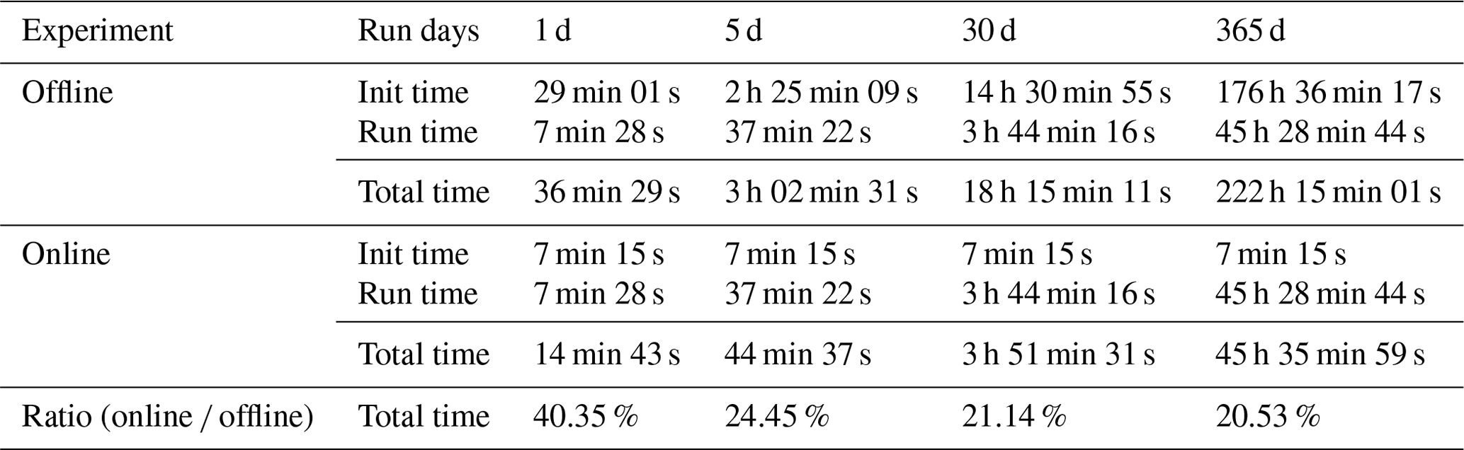
Init time is the initialization period + the input period. Run time is the model period + the analysis period + the output period.
It takes about 36 min 29 s to run 1 d offline cda, but it only takes about 14 min 43 s to run a 1 d online cda experiment. A 30 d offline cda experiment takes 18 h 15 min 11 s, and the online experiment only takes 3 h 51 min 31 s. The CPU time of online assimilation is only 21.14 % of offline assimilation. Indeed, a 365 d online cda takes about 20.53 % of offline cda time. If the reanalyses are carried out over decades, the efficiency of online assimilation will be much higher than the offline mode. Again, depending on the performance of the HPC system, the I/O process wall clock time may take much more time through offline assimilation.
The results of the perfect twin experiments show that the CESM-ECDA system can work well. To further verify its performance in the real world, a 3-year reanalysis experiment (hereafter referred to as real-CDA) from 1978 to 1980 (1-year ODA and 2-year CDA) with the component setting of BHISTC5 is conducted using 12 ensemble members. Surface pressure from ERA-Interim (Dee et al., 2011), gridded observational SST from HadISST (Rayner et al., 2003), and three-dimensional temperature and salinity profiles from XBT, CTD, MBT, and OSD are assimilated. Considering that observations below 2000 m are very sparse, and internal variability in the deep ocean is weak, we employ global restoration of climatological temperature and salinity (e.g., Levitus et al., 2001, 2005, 2012) in the deep ocean to relax the distorted ocean stratification caused by strong data constraints in upper ocean (Lu et al., 2020). A control experiment (hereafter referred to as real-CTL) is also conducted with the same setup, except that it does not employ data assimilation.
We compare the Ps and SST results of real-CDA with those of CFSR (Saha et al., 2010), 20CRv2 (Compo et al., 2011), 20CRv3 (Slivinski et al., 2019), ERA-20C (Poli et al., 2013), and CERA-20C (Laloyaux et al., 2018) in Fig. 15a–d for 1980. The RMSE of Ps in real-CDA (red line) is smaller than real-CTL (black line) and 20CRv2 (yellow) but larger than the CFSR (purple line), ERA-20C (pink line), and 20CRv3 (green line). The mean RMSEs of real-CTL, real-CDA, CFSR, 20CRv2, ERA-20C, and 20CRv3 are 15.57, 11.84, 9.21, 13.89, 6.68, and 4.82 hPa, respectively. In these reanalysis products, the RMSE of 20CRv3 is the smallest if we take ERA-Interim as truth.
The RMSE of SST in real-CDA is smaller than real-CTL (black) and CERA-20C (pink line) and close to CFSR (purple line). The mean RMSEs are 1.41, 0.16, 0.16, and 0.80∘ in real-CTL, real-CDA, CFSR, and CERA-20C, respectively. From the distributions in Fig. 15c–d, we see that the globally averaged Ps RMSE in real-CDA decreases 30 %–50 % compared to real-CTL in addition to Africa. Compared with CERA-20C, the SST RMSE is greatly reduced worldwide to an extent of about 30 %–90 %. Here, we are not saying that the results of real-CDA are better than CERA-20C because the SST in CERA-20C is relaxed toward the HadISST2 monthly ensemble product (Laloyaux et al., 2018). The limited results in Fig. 15 only show the effectiveness of the CESM-ECDA system. More real-observation assimilation experiments and more comprehensive verification analysis will be carried out in future work.
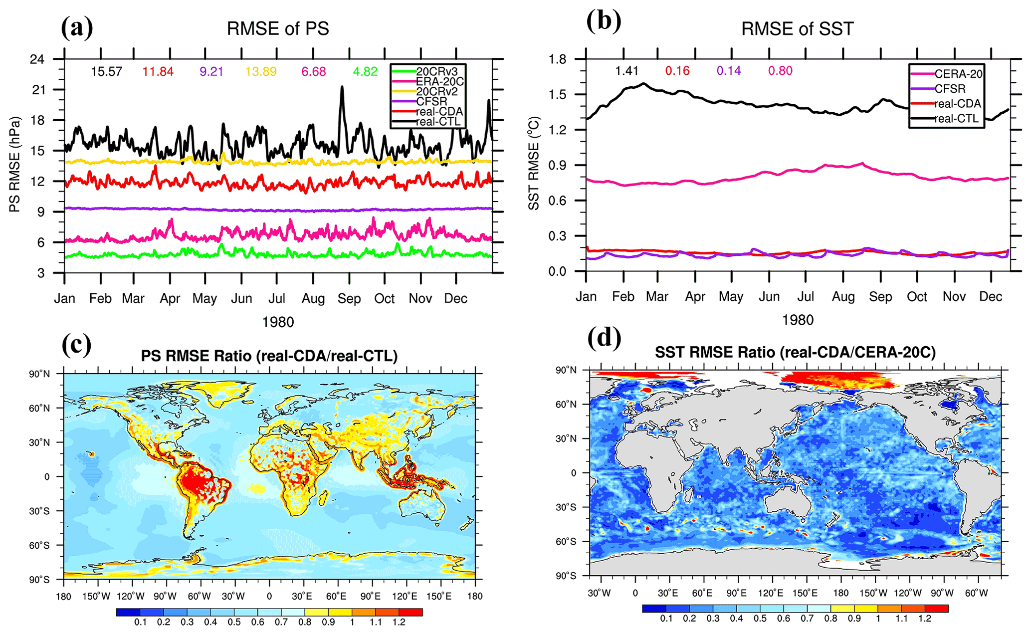
Figure 15Time series of RMSE of (a) Ps and (b) SST from the real-observation assimilation experiment and RMSE ratio distributions of Ps (real-CDA/real-CTL) and SST (real-CDA/CERA-20C) in 1980. The numbers in (a) and (b) are RMSEs of the mean value corresponding to each product.
In this paper, an online ensemble atmosphere–ocean coupled data assimilation system within the Community Earth System Model, which consists of the ODA component and the ADA components (both for the finite-volume and the spectral-element dynamical cores for ADA), is designed and evaluated systematically. In the ADA component, the surface pressure observations are assimilated. In the ODA component, the gridded SST observations and the in situ profiles of temperature and salinity are both assimilated. The perfect twin experiments have been conducted steadily for 1 model year for the single ADA components, the single ODA component, and the weakly coupled CESM-ECDA system. The results show that the CESM-ECDA system is effective in assimilating observations in both atmosphere and ocean. By assimilating the surface pressure observations alone, the RMSEs are significantly reduced by up to 39 % for Ps and 16 %–26 % for Ts, Qs, Us, and Vs within CAM-FV. The RMSE reductions for the single ADA experiment within CAM-SE are generally smaller but still more significant than those in CAM-FV. By assimilating the SST observations alone, the SST RMSE is greatly reduced by up to 77 %. When the three-dimensional in situ temperature and salinity profiles are further assimilated in the ODA system, the three-dimensional ocean temperature and salinity can be significantly improved.
When the atmospheric and oceanic observations are jointly assimilated, the CESM-ECDA system executes in a WCDA style. Results show that the CESM-ECDA system can obtain robustly improved state estimations in both atmosphere and ocean compared with the corresponding single-component DA experiments discussed above, respectively, which confirms the stability and effectiveness of the established CESM-ECDA system. The atmosphere–ocean coupled assimilation allows us to make more effective use of the available observations in both atmosphere and ocean components. Therefore, the observational information in different component systems is allowed to be transmitted and exchanged across the air–sea interface in the forecast stage of the coupled model. It is worth mentioning that due to the significant difference of the characteristic spatial and temporal scales between the atmosphere and the ocean and the difference of the air–sea coupling mechanisms in different regions, the coupled state estimation obtained shows a more complicated distribution.
This study also introduces and compares the offline and online assimilation approaches. A test which assimilates SST and TS profiles once a day and Ps four times a day shows that the online assimilation can save about 80 % CPU time, which will greatly improve the efficiency of long-term climate reanalysis. Furthermore, the reanalysis experiment with real observations shows that the Ps RMSE of CESM-ECDA is smaller than 20CRv2 if we take ERA-Interim as truth. The SST RMSE of CESM-ECDA is smaller than CERA-20C and close to CFSR when HadISST is assimilated.
A previous adaptively inflated ensemble filter study has been designed to enhance the consistency of upper- and deep-ocean adjustments, which is based on “climatological” standard deviations being adaptively updated by observations (Zhang and Rosati, 2010). But in this study, we only focus on the system design and evaluation of the CESM-ECDA; the inflation is not used in this study. The inflation scheme can be considered into the ADA system in the next work. While in ocean, the situation is more complex because the variability is different in upper and deep ocean. It needs much deeper and further work to explore the inflation in this CESM-ECDA system.
In this study, our purpose is to document the design and evaluation of the online CESM-ECDA system instead of providing a climate reanalysis product. Only several 1-year perfect twin experiments and a 3-year analysis experiment with real observations are conducted. In follow-up studies, we plan to complete a half-century climate reanalysis with an improved CDA system using ensemble optimal interpolation (EnOI)-like filtering (Yu et al., 2019), which can effectively solve the problem of redistribution between model integration and assimilation, in which only one dynamical model member is integrated.
The online CESM-ECDA system reported in this study uses multiple ensemble members to carry out the assimilation process. The required computing resources are large for such an ensemble-based CDA system with the full-complexity CGCM to execute, especially when using a high-resolution configuration (e.g., the CESM-HR, Zhang et al., 2020a). In addition, observations of other types and variables need to be further assimilated into the system. Further, the current CESM-ECDA system is only a weakly coupled system in which the observations in one component cannot directly update the state in another component. It is worth mentioning that some ocean dynamic processes (particularly in the tropics, such as ENSO, the El Niño–Southern Oscillation) have influences over a long spatial scale. However, depending on the reliability of statistical correlation, such as the ensemble size, the localization radius is a tunable parameter in practical data assimilation. Considering the compressibility and that the Rossby radius of deformation in the atmosphere is generally larger than the ocean, the impact radius of atmosphere is larger than the ocean in this work. We highlight here that an appropriate utilization of localization is important in the real-observation data assimilation and coupled reanalysis, which shall be further explored.
It is worth mentioning that a high-resolution configuration of CESM has been performed and evaluated thoroughly for century-long climate simulations (Small et al., 2014; Zhang et al., 2020a) and participated in the High-Resolution Model Intercomparison Project (HighResMIP; Roberts et al., 2020). A 500-year preindustrial control simulation and a 250-year historical and future climate simulation have also been completed and evaluated (Zhang et al., 2020a; Chang et al., 2020). In this paper, the CESM-ECDA system is only evaluated with a standard resolution. In the future, the CESM-ECDA system will be assessed with the high-resolution version of CESM. Referring to the multi-timescale EnOI-like high-efficiency approximate filter (Yu et al., 2019), our ultimate goal is to develop a computationally efficient CDA system suitable for the CESM-HR (e.g., 25 km ADA system within CAM-SE and 10 km ODA system within POP2) using only one CESM integration instead of multiple ensemble members. This CDA system with CESM-HR is expected to be used to produce a high-resolution coupled reanalysis using various real observations. Therefore, much work remains to be done in the future. The ability to assimilate real observations of various types needs to be included in the future, by which similarities and differences with the previous studies (e.g., Zhang et al., 2007; Lu et al., 2020) can be compared, and important climate phenomena such as ENSO and the Atlantic meridional overturning circulation (AMOC) can also be further explored. In addition, the cross-domain coupled error covariance is desired to be included in the future to extend the current weakly CDA system to a strongly CDA one.
The codes of the CESM-ECDA system and the data used in this work are available at Zenodo via https://doi.org/10.5281/zenodo.5733849 (Jiang et al., 2021).
SZ, WZ, JS, and YJ initiated this research, proposed most ideas, and co-led the writing of the paper.
JS and YJ led the process of development and research and contributed equally to this work as co-first authors.
All authors contributed to the improvement of ideas, software testing, experimental evaluation, and writing of the paper and proofreading.
The contact author has declared that neither they nor their co-authors have any competing interests.
Publisher's note: Copernicus Publications remains neutral with regard to jurisdictional claims in published maps and institutional affiliations.
We thank the anonymous reviewers, for their thorough examinations and useful and helpful comments on the early version of the paper. The reanalysis data and observations used to do the comparison are from ECMWF (https://www.ecmwf.int/en/forecasts/datasets, last access: 28 November 2021), 20CRv2c, (https://rda.ucar.edu/datasets/ds131.2/, last access: 28 November 2021), CFSR, (https://rda.ucar.edu/datasets/ds093.1/, last access: 28 November 2021).
The research is supported by the Chinese NFS projects 41830964, 41775100, and 311021009 and the Key R&D program of Ministry of Science and Technology of China (2017YFC1404100, 2017YFC1404104, and 2018YFC1406202), as well as Shandong Province's Taishan Scholars Program (ts201712017) and the Qingdao “Creative and Initiative” Frontier Scientist Program (19-3-2-7-zhc).
This paper was edited by Charles Onyutha and reviewed by two anonymous referees.
Anderson, J. L.: An ensemble adjustment Kalman filter for data assimilation, Mon. Weather Rev., 129, 2884–2903, 2001.
Anderson, J. L.: A local least squares framework for ensemble filtering, Mon. Weather Rev., 131, 634–642, 2003.
Anderson, J. L. and Anderson, S. L.: A monte carlo implementation of the nonlinear filtering problem to produce ensemble assimilations and forecasts, Mon. Weather Rev., 127, 2741–2758, 1999.
Anderson, J. L., Wyman, B., Zhang, S., and Hoar, T.: Assimilation of surface pressure observations using an ensemble filter in an idealized global atmospheric prediction system, J. Atmos. Sci., 62, 2925–2938, 2005.
Anderson, J. L. and Collins N.: Scalable Implementations of Ensemble Filter Algorithms for Data Assimilation, J. Atmo. Ocean Tech., 24, 1452–1463, https://doi.org/10.1175/JTECH2049.1, 2007.
Anderson, J., Hoar, T., Raeder, K., Liu, H., Collins, N., Torn, R., and Arellano, A.: The Data Assimilation Research Testbed: A community facility, B. Am. Meteorol. Soc., 90, 1283–1296, https://doi.org/10.1175/2009BAMS2618.1, 2009.
Arblaster, J. M., Meehl, G. A., and Karoly, D. J.: Future climate change in the Southern Hemisphere: Competing effects of ozone and greenhouse gases, Geophys. Res. Lett., 38, L02701, https://doi.org/10.1029/2010GL045384, 2011.
Asefi-Najafabady, S., Vandekar, K., Seimon, A., Lawrence, P., and Lawrence, D.: Climate change, population and poverty: vulnerability and exposure to heat stress in East Africa, Climatic Change, 148, 561–573, https://doi.org/10.1007/s10584-018-2211-5, 2018.
Balmaseda, M. and Anderson, D.: Impact of initialization strategies and observations on seasonal forecast skill, Geophys. Res. Lett., 36, L01701, https://doi.org/10.1029/2008GL035561, 2009.
Bitz, C. M.: Some aspects of uncertainty in predicting sea ice retreat, in: Arctic Sea Ice Decline: observations, projections, mechanisms, and implications, edited by: deWeaver, E., Bitz, C. M., and Tremblay, B., AGU Geophysical Monograph Series, American Geophysical Union, 180, 63–76, 2008.
Bloom, S. C., Takacs, L. L., da Silva, A. M., and Ledvina, D.: Data assimilation using incremental analysis updates, Mon. Weather Rev., 124, 1256, https://doi.org/10.1175/1520-0493(1996)124<1256:DAUIAU>2.0.CO;2, 1996.
Browne, P. A. and Leeuwen, P. J. van: Twin experiments with the equivalent weights particle filter and HadCM3, Q. J. Roy. Meteor. Soc., 141, 3399–3414, https://doi.org/10.1002/qj.2621, 2015.
Browne, P. A. and Wilson, S.: A simple method for integrating a complex model into an ensemble data assimilation system using MPI, Environ. Modell. Softw., 68, 122–128, 2015.
Browne, P. A., Rosnay, P., Zuo H., Bennett, A., and Dawson, A.: Weakly Coupled Ocean–Atmosphere Data Assimilation in the ECMWF NWP System, Remote Sens., 11, 234, https://doi.org/10.3390/rs11030234, 2019.
Carton, J. A., Chepurin, G. A., and Chen, L.: SODA3: A New Ocean Climate Reanalysis, J. Climate, 31, 6967–6983, https://doi.org/10.1175/JCLI-D-18-0149.1, 2018.
Chandan, D. and Peltier, W. R.: On the mechanisms of warming the mid-Pliocene and the inference of a hierarchy of climate sensitivities with relevance to the understanding of climate futures, Clim. Past, 14, 825–856, https://doi.org/10.5194/cp-14-825-2018, 2018.
Chang, P., Zhang, S., Danabasoglu, G., Yeager, S. G., Fu, H., Wang, H., et al.: An unprecedented set of high-resolution earth system simulations for understanding multiscale interactions in climate variability and change, J. Adv. Model. Earth Sy., 12, e2020MS002298, https://doi.org/10.1029/2020MS002298, 2020.
Cheng, W., Curchitser, E., Ladd, C., Stabeno, P., and Wang, M.: Influences of sea ice on the Eastern Bering Sea: NCAR CESM simulations and comparison with observations, Deep-Sea Res. Pt. II, 109, 27–38, https://doi.org/10.1016/j.dsr2.2014.03.002, 2014.
Chiodo, G., Garcia-Herrera, R., Calvo, N., Vaquero, J. A., Añel, and Matthes, K.: The impact of a future solar minimum on climate change projections in the Northern Hemisphere, Environ. Res. Lett., 11, 034015 https://doi.org/10.1088/1748-9326/11/3/034015, 2016.
Coelho, C. A. S. and Goddard, L.: El Niño–induced tropical droughts in climate change projections, J. Climate, 22, 6456–6476, https://doi.org/10.1175/2009JCLI3185.1, 2009.
Collins, M.: Climate predictability on interannual to decadal time scales: The initial value problem, Clim. Dynam., 19, 671–692, 2002.
Compo, G. P., Whitaker, J. S., Sardeshmukh, P. D., et al.: The Twentieth Century Reanalysis Project, Q. J. Roy. Meteor. Soc., 137, 1–28, https://doi.org/10.1002/qj.776, 2011.
Danabasoglu, G., Lamarque, J. F., Bacmeister, J., et al.: The Community Earth System Model version 2 (CESM2), J. Adv. Model. Earth Sy., 12, e2019MS001916, https://doi.org/10.1029/2019MS001916, 2020.
Dee, D., Uppala, S. M., Simmons, A. J., et al.: The ERA-Interim reanalysis: Configuration and performance of the data assimilation system, Q. J. Roy. Meteor. Soc., 137, 553–597, https://doi.org/10.1002/qj.828, 2011.
Dennis, J. M., Edwards, J., Evans, K. J., Guba, O., Lauritzen, P. H., Mirin, A. A., St-Cyr, A., Taylor, M. A., and Worley P. H.: CAM-SE: A scalable spectral element dynamical core for the Community Atmosphere Model, Int. J. High Perform. C, 26, 74–89, https://doi.org/10.1177/1094342011428142, 2012.
Derber, J. and Rosati, A.: A global oceanic data assimilation system, J. Phys. Oceanogr., 19, 1333–1347, 1989.
Evans, K. J., Lauritzen, P. H., Mishra, S. K., Neale, R. B., Taylor, M. A., and Tribbia, J. J.: AMIP Simulation with the CAM4 Spectral Element Dynamical Core, J. Climate, 26, 689–709, https://doi.org/10.1175/JCLI-D-11-00448.1, 2013.
Evensen, G.: Sequential data assimilation with a nonlinear quasi-geostrophic model using Monte Carlo methods to forecast error statistics, J. Geophys. Res., 99, 10143–10162, https://doi.org/10.1029/94JC00572, 1994.
Evensen, G.: The ensemble Kalman filter: Theoretical formulation and practical implementation, Ocean Dynam., 53, 343–367, https://doi.org/10.1007/s10236-003-0036-9, 2003.
Fasullo, J. T. and Nerem, R. S.: Interannual variability in global mean sea level estimated from the CESM large and last millennium ensembles, Water, 8, 491, https://doi.org/10.3390/w8110491, 2016.
Gantt, B., He, J., Zhang, X., Zhang, Y., and Nenes, A.: Incorporation of advanced aerosol activation treatments into CESM/CAM5: model evaluation and impacts on aerosol indirect effects, Atmos. Chem. Phys., 14, 7485–7497, https://doi.org/10.5194/acp-14-7485-2014, 2014.
Gaspari, G. and Cohn, S. E.: Construction of correlation functions in two and three dimensions, Q. J. Roy. Meteor. Soc., 125, 723–757, https://doi.org/10.1002/qj.49712555417, 1999.
Glotfelty, T., He, J., and Zhang, Y.: The impact of future climate policy scenarios on air quality and aerosol/cloud interactions using an advanced version of CESM/CAM5. Part II: Future trend analysis and impacts of projected anthropogenic emissions, Atmos. Environ., 152, 531–552, 2017.
Goldenson, N., Doherty, S. J., Bitz, C. M., Holland, M. M., Light, B., and Conley, A. J.: Arctic climate response to forcing from light-absorbing particles in snow and sea ice in CESM, Atmos. Chem. Phys., 12, 7903–7920, https://doi.org/10.5194/acp-12-7903-2012, 2012.
Goosse, H. and Holland, M. M.: Mechanisms of interdecadal Arctic climate variability in the Community Climate System Model CCSM2, J. Climate, 18, 3552–3570, 2005.
Gropp, W., Lusk, E., Doss, N., and Skjellum, A.: A high-performance, portable implementation of the mpi message passing interface standard, Parallel Comput., 22, 789–828, 1996.
Gropp, W., Lusk, E., and Thakur, R.: Using MPI-2: Advanced Features of the Message-Passing Interface, MIT Press, 1999.
Han, G., Wu, X., Zhang, S., Liu, Z., and Li, W.: Error covariance estimation for coupled data assimilation using a Lorenz atmosphere and a simple pycnocline ocean model, J. Climate, 26, 10218–10231, 2013.
Hunke, E. C. and Lipscomb, W. H.: CICE: The Los Alamos sea ice model user's manual, version 4, Los. Alamos. National Laboratory Tech. Rep., LA-CC-06-012, 2008.
Jiang, Y., Zhang, S., and Sun, J.: Program codes and main data for the paper “An Online Ensemble Coupled Data Assimilation Capability for the Community Earth System Model: System Design and Evaluation”, Zenodo [code and data set], https://doi.org/10.5281/zenodo.5733849, 2021.
Karspeck, A. R., Yeager, S., Danabasoglu, G., Hoar, Y., Collins, N., Raeder, K., Anderson, J., and Tribbia, J.: An Ensemble Adjustment Kalman filter for the CCSM4 ocean component, J. Climate, 26, 7392–7413, 2013.
Karspeck, A. R., Danabasoglu, G., Anderson, J., Karol, S., Karol, S., Collins, N., Vertenstein, M., Raeder, K., Hoar, T., Neale, R., Edwards, J., and Craig, A.: A global coupled ensemble data assimilation system using the community earth system model and the data assimilation research testbed, Q. J. Roy Meteor. Soc., 144, 2304–2430, https://doi.org/10.1002/qj.3308, 2018.
Kleist, D. T., Parrish, D. F., Derber, J. C., Treadon, R., Wu, W.-S., and Lord, S.: Introduction of the GSI into the NCEP Global Data Assimilation System, Mon. Weather Rev., 24, 1691–1705, 2009.
Laloyaux, P., Balmaseda, M., Dee, D., Mogensen, K., and Janssen P.: A coupled data assimilation system for climate reanalysis, Q. J. Roy. Meteor. Soc., 142, 65–78, https://doi.org/10.1002/qj.2629, 2016.
Lawrence, D. M., Oleson, K. W., Flanner, M. G., et al.: Parameterization improvements and functional and structural advances in version 4 of the Community Land Model, J. Adv. Model. Earth Sy., 3, MS000045, https://doi.org/10.1029/2011MS00045, 2011.
Levitus, S., Antonov, J. I., Wang, J., Delworth, T. L., Dixon, K. W., and Broccoli, A. J.: Anthropogenic warming of Earth's climate system, Science, 292, 267–270, 2001.
Levitus, S., Antonov, J. I., and Boyer, T. P.: Warming of the world ocean, 1955–2003, Geophys. Res. Lett., 32, L02604, https://doi.org/10.1029/2004GL021592, 2005.
Levitus, S., Antonov, J. I., Boyer, T. P., Baranova, O. K., and Zweng, M. M.: World ocean heat content and thermosteric sea level change (0–2000 m), 1955–2010, Geophys. Res. Lett., 39, L10603, https://doi.org/10.1029/2012GL051106, 2012.
Lu, F., Liu, Z., Zhang, S., and Liu, Y.: Strongly coupled data assimilation using leading averaged coupled covariance (LACC). Part II: CGCM applications, Mon. Weather Rev., 143, 4645–4659, 2015.
Lu, L., Zhang, S., Yeager, S. G., Danabasoglu, G., Chang, P., Wu, L., Lin, X., Rosati, A., and Lu, F.: Impact of coherent ocean stratification on AMOC reconstruction by coupled data assimilation with a biased model, J. Climate, 33, 7319–7334, https://doi.org/10.1175/JCLI-D-19-0735.1, 2020.
Mu, L., Nerger, L., Tang, Q., Loza, S. N., Sidorenko, D., Wang, Q., Semmler, T., Zampieri, L., Losch, M., and Goessling, H. F.: Toward a Data Assimilation System for Seamless Sea Ice Prediction Based on the AWI Climate Model, J. Adv. Model. Earth Sy., 12, e2019MS001937, https://doi.org/10.1029/2019MS001937, 2020.
Neale, R. B., Gettelman, A., Park, S., Conley, A. J., Kinnison, D., Dan, M., Smith, A. K., Vitt, F., Morrison, H., and Cameronsmith P.: Description of the NCAR Community Atmosphere Model (CAM 5.0), NCAR Tech. Note NCAR/TN-486+STR, 1–289, Boulder, CO, National Center for Atmospheric Research, 2012.
Nerger, L. and Hiller, W.: Software for Ensemble-based Data Assimilation Systems – Implementation Strategies and Scalability, Comput. Geosci., 55, 110–118, 2013.
Nerger, L., Tang, Q., and Mu, L.: Efficient ensemble data assimilation for coupled models with the Parallel Data Assimilation Framework: example of AWI-CM (AWI-CM-PDAF 1.0), Geosci. Model Dev., 13, 4305–4321, https://doi.org/10.5194/gmd-13-4305-2020, 2020.
Penny, S. G., Akella, S., Buehner, M., Chevallier, M., Counillon, F., Draper, C., Frolov, S., Fujii, Y., Karspeck, A., Kumar, A., et al.: “Coupled Data Assimilation for Integrated Earth System Analysis and Prediction: Goals, Challenges and Recommendations”, WMO, WWRP 2017-3, 2017.
Raeder, K., Anderson, J. L., Collins, N., Hoar, T. J., and Pincus, R.: DART/CAM: an ensemble data assimilation system for cesm atmospheric models, J. Climate, 25, 6304–6317, 2012.
Rayner, N., Parker, D. E., Horton, E. B., Folland, C. K., Alexander, L. V., and Rowell, D. P.: Global analyses of sea surface temperature, sea ice, and night marine air temperature since the late nineteenth century, J. Geophys. Res.-Atmos., 108, 4407, https://doi.org/10.1029/2002JD002670, 2003.
Roberts, M. J., Jackson, L. C., Roberts, C. D., et al.: Sensitivity of the Atlantic meridional overturning circulation to model resolution in CMIP6 HighResMIP simulations and implications for future changes, J. Adv. Model. Earth Sy., 12, e2019MS002014, https://doi.org/10.1029/2019MS002014, 2020.
Rosati, A., Miyakoda, K., and Gudgel, R.: The impact of ocean initial conditions on ENSO forecasting with a coupled model, Mon. Weather Rev., 125, 754–772, 1997.
Saha, S., Nadiga, S., Thiaw, C., and Wang, J.: The NCEP climate forecast system, J. Climate, 27, 2185–2208, https ://doi.org/10.1175/JCLI3812.1, 2006.
Saha, S., Moorthi, S., Pan H.-L., et al.: The NCEP Climate Forecast System Reanalysis, B. Am. Meteorol. Soc., 91, 1015–1058, https://doi.org/10.1175/2010BAMS3001.1, 2010.
Skachko, S., Buehner, M., Laroche, S., Lapalme, E., Smith, G., Roy, F., Surcel-Colan, D., Bélanger, J.-M., and Garand, L.: Weakly coupled atmosphere–ocean data assimilation in the Canadian global prediction system (v1), Geosci. Model Dev., 12, 5097–5112, https://doi.org/10.5194/gmd-12-5097-2019, 2019.
Slivinski, L. C., Compo, G. P., Whitaker, J. S., et al.: Towards a more reliable historical reanalysis: Improvements for version 3 of the Twentieth Century Reanalysis system, Q. J. Roy. Meteor. Soc., 145, 2876–2908, https://doi.org/10.1002/qj.3598, 2019.
Small, R. J., Bacmeister, J., Bailey, D., et al.: A new synoptic scale resolving global climate simulation using the community earth system model, J. Adv. Model. Earth Sy., 6, 1065–1094, https://doi.org/10.1002/2014MS000363, 2014.
Smith, R. D., Jones, P., Briegleb, B., et al.: The parallel ocean program (POP) reference manual, Los Alamos National Laboratory tech. Rep. LAUR-10-01853, 2010.
Poli, P., Hersbach, H., Tan, D. G. H., et al.: The data assimilation system and initial performance evaluation of the ECMWF pilot reanalysis of the 20th-century assimilating surface observations only (ERA-20C), ECMWF ERA Rep. 14, 59 pp., 2013.
Tang, Q., Mu, L., Sidorenko, D., Goessling, H., Semmler, T., and Nerger, L.: Improving the ocean and atmosphere in a coupled ocean–atmosphere model by assimilating satellite sea-surface temperature and subsurface profile data, Q. J. Roy. Meteor. Soc., 146, 4014–4029, 2020.
Tippett, M. K., Anderson, J. L., Bishop, C. H., Hamill, T. M., and Whitaker, J. S.: Ensemble square root filters, Mon. Weather Rev., 131, 1485–1490, 2003.
Whitaker, J. S., Compo, G. P., Wei, X., and Hamill, T. M.: Reanalysis without radiosondes using ensemble data assimilation, Mon. Weather Rev., 132, 1190–1200, 2004.
Yang, X., Delworth, T. L., Zeng, F., Zhang, L., Cooke, W. F., Harrison, M. J., Rosati, A., Underwood, S., Compo, G. P., and McColl, C.: On the Development of GFDL's decadal prediction system: initialization approaches and retrospective forecast assessment, J. Adv. Model. Earth Sy., 13, e2021MS002529, https://doi.org/10.1029/2021MS002529, 2021.
Yu, X., Zhang, S., Li, J., Lu, L., Liu, Z., Li, M., Yu, H., Han, G., Lin, X., Wu, L., and Chang, P.: A multi-timescale EnOI-Like high-efficiency approximate filter for coupled model data assimilation, J. Adv. Model. Earth Sy., 11, 45–63, https://doi.org/10.1029/2018MS001504, 2019.
Zhang, F. Q., Snyder, C., and Sun, J.: Impacts of initial estimate and observation availability on convective-scale data assimilation with an ensemble kalman filter, Mon. Weather Rev., 132, 1–16, 2004.
Zhang, S.: A study of impacts of coupled model initial shocks and state-parameter optimization on climate prediction using a simple pycnocline prediction model, J. Climate, 24, 6210–6226, 2011.
Zhang, S. and Anderson, J. L.: Impact of spatially and temporally varying estimates of error covariance on assimilation in a simple atmospheric model, Tellus A, 55, 126–147, 2003.
Zhang, S. and Rosati, A.: An Inflated Ensemble Filter for Ocean Data Assimilation with a Biased Coupled GCM, Mon. Weather Rev., 138, 3905–3931, https://doi.org/10.1175/2010MWR3326.1, 2010.
Zhang, S., Harrison, M. J., Wittenberg, A. T., Rosati, A., Anderson, J. L., and Balaji, V.: Initialization of an ENSO forecast system using a parallelized ensemble filter, Mon. Weather Rev., 133, 3176–3201, 2005.
Zhang, S., Harrison, M. J., Rosati, A., and Wittenberg, A.: System design and evaluation of coupled ensemble data assimilation for global oceanic climate studies, Mon. Weather Rev., 135, 3541–3564, https://doi.org/10.1175/MWR3466.1, 2007.
Zhang, S., Rosati, A., and Delworth, T.: The Adequacy of Observing Systems in Monitoring the Atlantic Meridional Overturning Circulation and North Atlantic Climate, J. Climate, 23, 5311–5324, 2010.
Zhang, S., Fu, H., Wu, L., Li, Y., Wang, H., Zeng, Y., Duan, X., Wan, W., Wang, L., Zhuang, Y., Meng, H., Xu, K., Xu, P., Gan, L., Liu, Z., Wu, S., Chen, Y., Yu, H., Shi, S., Wang, L., Xu, S., Xue, W., Liu, W., Guo, Q., Zhang, J., Zhu, G., Tu, Y., Edwards, J., Baker, A., Yong, J., Yuan, M., Yu, Y., Zhang, Q., Liu, Z., Li, M., Jia, D., Yang, G., Wei, Z., Pan, J., Chang, P., Danabasoglu, G., Yeager, S., Rosenbloom, N., and Guo, Y.: Optimizing high-resolution Community Earth System Model on a heterogeneous many-core supercomputing platform, Geosci. Model Dev., 13, 4809–4829, https://doi.org/10.5194/gmd-13-4809-2020, 2020a.
Zhang, S., Liu, Z., Zhang, X., et al.: Coupled data assimilation and parameter estimation in coupled ocean–atmosphere models: a review, Clim. Dynam., 54, 5127–5144, https://doi.org/10.1007/s00382-020-05275-6, 2020b.
- Abstract
- Copyright statement
- Introduction
- Model and filtering algorithm
- Development of online DA components with CESM
- The evaluation of CESM-ECDA system with perfect twin experiments
- The real-observation assimilation experiments
- Summary and discussions
- Code and data availability
- Author contributions
- Competing interests
- Disclaimer
- Acknowledgements
- Financial support
- Review statement
- References