the Creative Commons Attribution 4.0 License.
the Creative Commons Attribution 4.0 License.
 | 21 Jun 2022
The Comprehensive Automobile Research System (CARS) – a Python-based automobile emissions inventory model
Bok H. Baek
Rizzieri Pedruzzi
Minwoo Park
Chi-Tsan Wang
Younha Kim
Chul-Han Song
Jung-Hun Woo
The Comprehensive Automobile Research System (CARS) is an open-source Python-based automobile emissions inventory model designed to efficiently estimate high-quality emissions from motor vehicle emission sources. It can estimate air pollutant, greenhouse gas, and air toxin criteria at any spatial resolution based on the spatiotemporal resolutions of input datasets. The CARS is designed to utilize local vehicle activity data, such as vehicle travel distance, road-link-level network geographic information system (GIS) information, and vehicle-specific average speed by road type, to generate an automobile emissions inventory for policymakers, stakeholders, and the air quality modeling community. The CARS model adopted the European Environment Agency's on-road automobile emissions calculation methodologies to estimate the hot exhaust, cold start, and evaporative emissions from on-road automobile sources. It can optionally utilize average speed distribution (ASD) of all road types to reflect more realistic vehicle speed variations. In addition, through utilizing high-resolution road GIS data, the CARS can estimate the road-link-level emissions to improve the inventory's spatial resolution. When we compared the official 2015 national mobile emissions from Korea's Clean Air Policy Support System (CAPSS) against the ones estimated by the CARS, there is a significant increase in volatile organic compounds (VOCs) (33 %) and carbon monoxide (CO) (52 %) measured, with a slight increase in fine particulate matter (PM2.5) (15 %) emissions. Nitrogen oxide (NOx) and sulfur oxide (SOx) measurements are reduced by 24 % and 17 %, respectively, in the CARS estimates. The main differences are driven by different vehicle activities and the incorporation of road-specific ASD, which plays a critical role in hot exhaust emission estimates but was not implemented in Korea's CAPSS mobile emissions inventory. While 52 % of vehicles use gasoline fuel and 35 % use diesel, gasoline vehicles only contribute 7.7 % of total NOx emissions, whereas diesel vehicles contribute 85.3 %. However, for VOC emissions, gasoline vehicles contribute 52.1 %, whereas diesel vehicles are limited to 23 %. Diesel buses comprise only 0.3 % of vehicles and have the largest contribution to NOx emissions (8.51 % of NOx total) per vehicle due to having longest daily vehicle kilometer travel (VKT). For VOC emissions, compressed natural gas (CNG) buses are the largest contributor at 19.5 % of total VOC emissions. For primary PM2.5, more than 98.5 % is from diesel vehicles. The CARS model's in-depth analysis feature can assist government policymakers and stakeholders in developing the best emission abatement strategies.
- Article
(3324 KB) - Full-text XML
- BibTeX
- EndNote


Globally, ambient pollution causes more than 4.2 million premature deaths every year (Cohen et al., 2017), and Burnett et al. (2018) estimated the health burden is closer to 9 million deaths from ambient PM concentrations. To effectively mitigate air pollutants, governments have been implementing stringent air pollution control policies to reduce harmful regional air pollutants (Hogrefe et al., 2001a, b; Dennis et al., 2010; Rao et al., 2011; Appel et al., 2013; Luo et al., 2019). The chemical transport model (CTM) simulation results strongly rely on precise input data, such as emission inventory, meteorology, land surface parameters, and chemical mechanisms in the atmosphere.
The transportation sector is one of the major anthropogenic emission sources in urban areas. Tailpipe emissions from vehicle combustion processes contain many air pollutants, including nitrogen oxides (NOx), volatile organic compounds (VOCs), carbon monoxide (CO), ammonia (NH3), sulfur dioxide (SO2), and primary particulate matter (PM), which participate in the formation of detrimental secondary pollutants like ozone and PM2.5 in the atmosphere. In the Seoul Metropolitan Area (SMA) in South Korea, transportation automobile sources contribute the most to the total NOX and primary PM2.5 emissions across all emission sources (Choi et al., 2014; Kim et al., 2017a, b, c). Thus, it is critical to understand and better represent the emission patterns from transportation automobile sources in the CTM model. The use of process-based automobile emission models is highly recommended to meet the needs in CTM model because it can estimate high-resolution spatiotemporal automobile emissions (Moussiopoulos et al., 2009; Russell and Dennis, 2000).
There are two methodologies known in emission inventory development: top-down and bottom-up approaches. The choice of methods is determined by the input data availability. The top-down approach primarily relies on the aggregated and generalized country or regional information and is typically used in developing countries where only limited datasets and information are available. It has its limitations when representing the vehicle emission process realistically due to the lack of detailed activity and ancillary supporting data. However, the bottom-up approach requires higher-quality spatiotemporal activity datasets like road network information, vehicle composition (vehicle type, engine size, vehicle age, and fuel technology), pollutant-specific emissions factors, road segment length, traffic activity data, and fuel consumption (EEA, 2019; Ibarra-Espinosa et al., 2018; IEMA, 2017). It can generate more accurate and detailed automobile emissions across various operating processes, such as hot exhaust, evaporative, idling, and hot soak processes (Nagpure et al., 2016; Ibarra-Espinosa et al., 2018).
There are several bottom-up mobile emissions models available, like MOVES (MOtor Vehicle Emissions Simulator) from the U.S. Environmental Protection Agency (U.S. EPA), the COPERT (COmputer Programmed to calculate Emissions from Road Transport) model from the European Environment Agency (EEA), HERMES (High-Elective Resolution Modelling Emission System) from Barcelona Supercomputing Center (Guevara et al., 2019), the VEIN (Vehicular Emissions INventory) model developed by Ibarra-Espinosa et al. (2017), and the VAPI (Vehicular Air Pollution Inventory) model developed by Nagpure and Gurjar (2016) for India (Nagpure et al., 2016). While these models are all bottom-up emission inventory models, a single model cannot meet all modelers, policymakers, and stakeholders' needs because each model holds its own pros and cons. They are developed differently to meet specific user needs based on the types of traffic activity and emission factors, emission calculation methodologies, and other traffic-related inputs, such as average speed distribution and geographical resolution. Each model is developed with different levels of specificity, underlying datasets, and modeling assumptions.
The MOVES model has the ability to generate high-quality emissions for up to 16 different emission processes (running exhaust, start exhaust, evaporative, refueling, extended idling, brake, tire, etc.). It can simulate not only county-level but also road-segment-level emissions depending on data availability. It can also reflect local meteorological conditions, such as ambient temperature and relative humidity, which can significantly impact both pollutants and emissions processes (Choi et al., 2017; Perugu et al., 2018). One major disadvantage of this model is that it is difficult to update and apply to countries outside of the US because it has a high degree of specificity. The COPERT model, widely used in European countries, can model emissions at high resolution, is fully integrated with the EEA's on-road vehicle emissions factors guidelines, and can generate a complete quality assurance (QA) and visualization summary (Ntziachristos et al., 2009). The cons are that it is a proprietary commercial licensed software, limited to EEA guidance, and challenging to modify and update with any key input datasets like the latest emission factors from non-European countries (Lejri et al., 2018; Rodriguez-Rey et al., 2021; Li et al., 2019; Lv et al., 2019; Smit et al., 2019).
HERMES and VEIN are both recently released bottom-up inventory models. They have their pros in that they are both open-source models based on open-source computing languages (Python and R), which provide transparency regarding the emission calculations with a considerable amount of data behind them (Ibarra-Espinosa et al., 2018; Guevara et al., 2019). Both models are driven by comma-separated value (CSV) formatted input files, making it very easy for users to modify the input datasets. They are also based on the EEA's emission calculation method and equipped with a complete QA and visualization tool based on Python and R libraries. However, it is not an easy task to develop the emission factors and other required input datasets for other countries and implement any control strategy plan feature to generate a responsive reduced emissions inventory.
Overall, there are multiple shortcomings in incorporating these bottom-up models into CTM studies. They require strong programming skills to operate, such as collecting and preparing the input data to fit the model requirements, configuring the model variables, and changing specific variables that may be embedded in the code. Another downside is that while the geographical administration-level (e.g., county-level) emissions inventory can be estimated by these models, it requires a third-party emissions processor like the SMOKE (Sparse Matrix Operator Kernel Emissions) modeling system (Baek and Seppanen, 2021) to process and generate spatially and temporally resolved emissions inputs for CTM. Some detailed information, like link-level hourly driving patterns, can be lost in the emissions processing steps.
There is no single model capable of meeting all the requirements across various spatial and temporal scales (Pinto et al., 2020). However, transparency, simplicity, and a user-friendly interface are requirements for those who mainly work in transportation policy and air quality modeling development (Fallahshorshani et al., 2012; Kaewunruen et al., 2016; Sallis et al., 2016; Sun et al., 2016; Tominaga and Stathopoulos, 2016). Thus, the ideal motor vehicle emissions modeling system would be computationally optimized, easy-to-use, and user-friendly in terms of its interface. Additionally, the model should easily adapt detailed local activity information and the state-of-the-art emission factors as inputs to represent them in the highest resolution possible both temporally and spatially.
We have developed the Comprehensive Automobile Research System (CARS) to meet these requirements, especially for the air quality research community, policymakers, and air quality modelers. The CARS is a stand-alone, fully modularized, computationally optimized, Python-based automobile emission model. The modularization improves the efficiency of processing times as once district and road-link-level annual, monthly, and daily total emissions are computed; the rest of the processes are optional. It can generate chemically speciated, spatially gridded, hourly emissions for CTMs without any third-party programs to develop the highest-quality CTM-ready emission inputs. Details on modularization will be discussed later. The CARS model can be easily adopted and is simple for users to add new functions or modules to in the future. The application of the CARS to South Korea will be described in detail later.
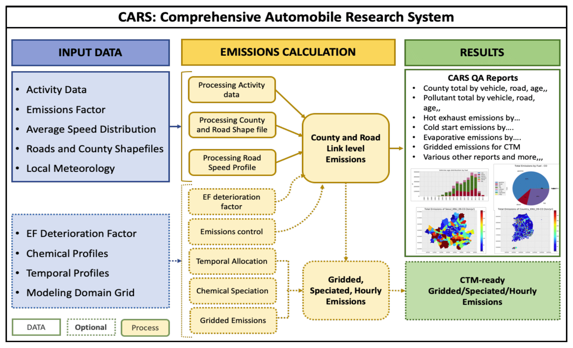
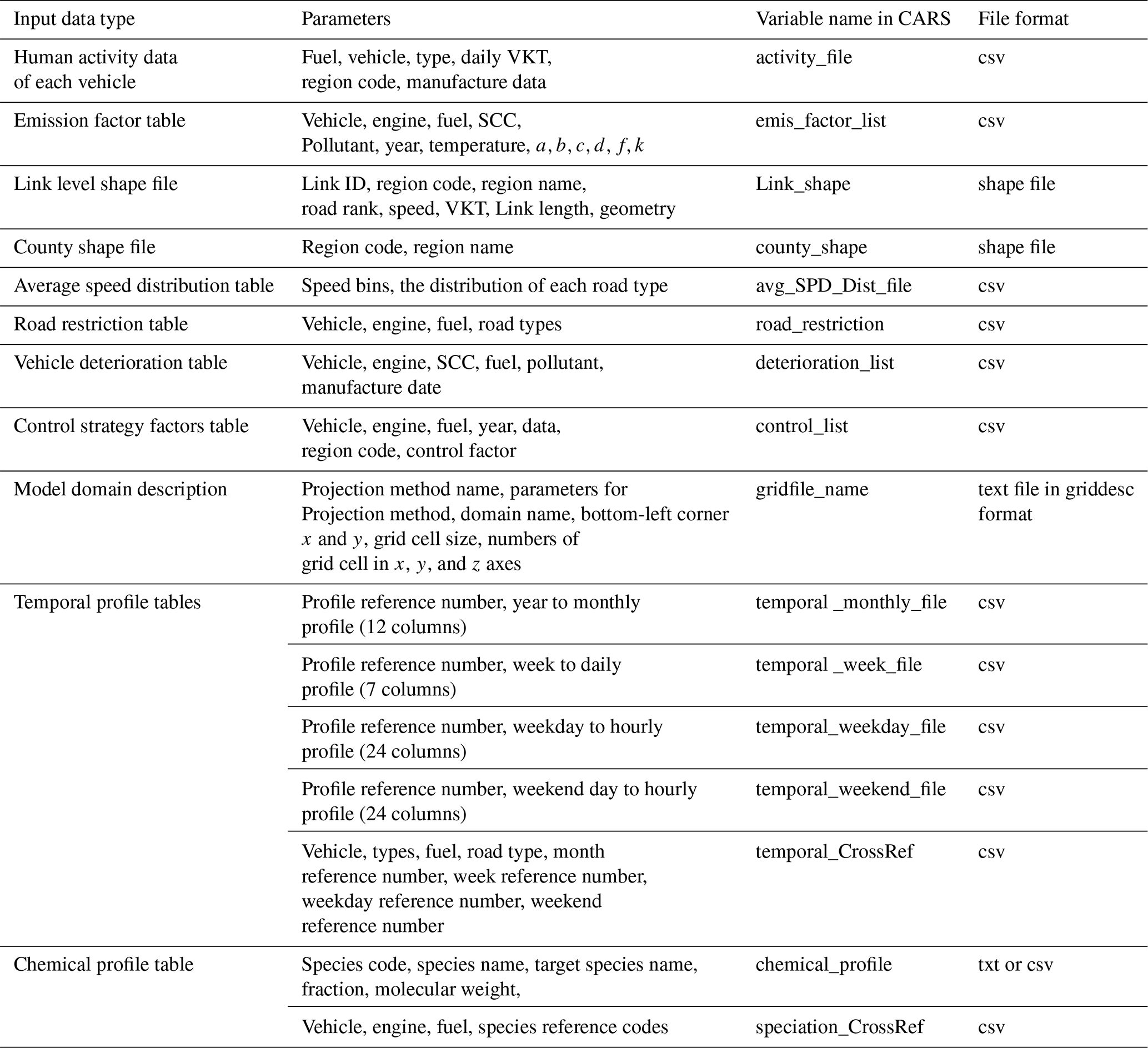
The CARS is an open-source Python-based customizable motor vehicle emissions processor that estimates on-road and off-road emissions for specific criteria and toxic air pollutants. Figure 1 is a schematic of the CARS overview. It applies vehicle-, engine-, and fuel-specific emission factors to traffic data to estimate the local-level annual, monthly, and daily total emissions inventory. The emissions inventory calculations require a list of pollutant-specific emissions factors by vehicle age, local activity data, average speed profile or distribution by road type, and geographic information system (GIS) road segment shapefile inputs. The spatial resolution of vehicle kilometer travel (VKT) determines the CARS geographic scale (i.e., district, county, state, and country) for emission calculations. Unlike the district-level Korea Clean Air Policy Support System (CAPSS) automobile emission inventory (Lee et al., 2011a, b), the CARS applies high-resolution annual average daily traffic (AADT) data from the road GIS shapefiles to distribute the total district emissions into road-link-level emissions. Optionally, these road-link-level emissions can be used to generate spatially gridded CTM-ready emissions input data once the output modeling domain is defined. The summary of input files by categories are presented in Appendix H. How the CARS estimates spatially and temporally enhanced automobile emissions inventories will be discussed in detail in Sect. 3.
South Korean traffic databases from the Korea National Institute of Environmental Research (NIER) CAPSS team (Lee et al., 2011b) were used in this study to compute the updated on-road automobile emissions inventory. The databases include individual vehicle activity data (daily total VKT), road activity data (average speed distribution by road), vehicle-age-specific emission factors, road type information, surface weather data, and GIS road shapefiles.
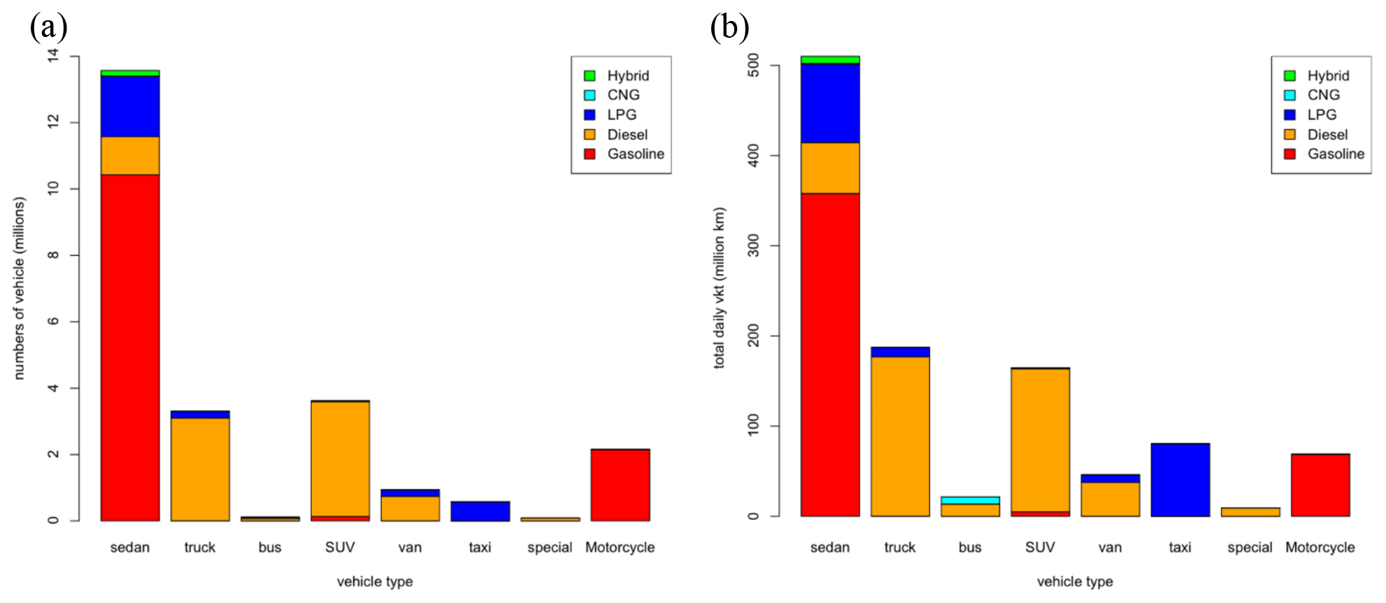
Figure 2(a) The number of vehicles by vehicle and fuel types and (b) the total daily VKT by vehicle and fuel type in South Korea.
2.1 Individual daily average VKT activity data
The individual vehicle VKT data is used to reflect human activity. This study imported the national registered vehicle-specific daily total VKT from South Korea's Vehicle Inspection Management System (VIMS), which belongs to the Korea Transportation Safety Authority (KTSA). It contains over 50 million records of vehicle-specific daily total VKT from 2013 to 2017. For the CARS model, we first sorted these records by the vehicle identification number (VIN) to remove any duplicates and then built vehicle-specific daily total VKT traffic activity data in the CSV format. The summary of those vehicle numbers and VKTs is presented in Fig. 2. Sedan vehicles using gasoline fuel comprise the greatest percentage of total vehicles at 47 % (∼10.4 million) and have the highest VKT. While most vehicles demonstrate a paired pattern between the number of vehicles and daily VKT, LPG (liquefied petroleum gas)-fueled taxis shows high VKT with low vehicle numbers due to their long-distance daily travel patterns.
The VIN (vin) information is used to calculate vehicle-specific daily average VKT (VKTvin, km d−1). In Eq. (1), the individual daily average vehicle VKT (VKTvin) is calculated based on the cumulative mileage (Mf;vin) between the last inspection date (Df;vin) and registration date (D0;vin). Each vehicle is categorized with Korea's NIER based on a combination of vehicle types (e.g., sedan, truck, bus), engine sizes (e.g., compact, full size, midsize), and fuel types (e.g., gasoline, diesel, LPG). Full details of vehicle types and daily total VKT are shown in Appendix A and B.
2.2 Emission calculations
Automobile emission sources include motorized engine sources on the paved road network and off the road network (e.g., driveways and parking lots). The CARS model does not currently simulate emissions from non-road emission sources, such as those from aviation, railways, construction, agriculture, lawnmowers, and boats. The CARS model simulates the on-road automobile emissions from network roads using their local traffic-related datasets. The following section explains the approach of the on-road automobile emission processes. The on-road emission (Eonroad) in the CARS is defined in Eq. (2), which includes three major emission processes (Ntziachristos and Samaras, 2000):
The “hot exhaust” emissions (Ehot) are the vehicle's tailpipe emissions when the internal combustion engine (ICE) combusts the fuel to generate energy under the average operating temperature. The “cold start” emissions (Ecold) are the tailpipe emissions from the ICE when the cold vehicle engine is ignited and the operational temperature is below the average conditions. The evaporative VOC emissions (Evap) are the emissions evaporated or permeated from the fuel systems (fuel tanks, injection systems, and fuel lines) of vehicles.
The CARS first applies the hot exhaust emission factors by vehicle type, age, fuel, engine, and pollutants to individual daily total VKT to compute the hot exhaust emissions. The rest of the processes for cold start and evaporative emissions are calculated afterwards. The emission calculation methodologies used in the CARS model are based on tier 2 and tier 3 methodologies from the EEA's mobile emission inventory guidebook (EEA, 2019) to be consistent with Korea's National Emission Inventory System (NEIS) (Lee et al., 2011a).
2.2.1 Hot exhaust emissions
Hot exhaust emissions are the exhaust gases produced by the combustion process in an ICE. The ICE combustion cycle generally causes incomplete combustion processes which emit hydrocarbons, carbon monoxide (CO), and particulate matter (PM). These are not completely controlled by the after-treatment equipment, such as a three-way catalytic converter, and released into the atmosphere. The sulfur compounds in the fuel are oxidized and become sulfur oxides (SOx). Nitrogen oxides (NOx) are produced due to the abundance of nitrogen (N2) and oxygen (O2) during the combustion process.
Equation (3) represents the calculation of daily individual vehicle hot exhaust emission rate, (g d−1), of the pollutant (p). An individual vehicle-specific daily VKTvin (km d−1) is estimated by Eq. (1). The EF (g km−1) is the hot exhaust emission factor of pollutants (p) for the vehicle type (v), vehicle manufacture year (vyr), and average vehicle speed (spd). The district's total emission rate is the total hot exhaust emissions from all individual vehicles within the same district.
The deterioration factor (DF) in Eq. (3) is an optional function in the CARS. The deterioration process is caused by vehicle aging and can lead to the increase of vehicle emissions. The vehicle DF is varied by vehicle type (v), pollutant (p), and vehicle manufacture year (vyr). The CARS model computes vehicle ages based on the vehicle manufacture year and model simulation year. According to NIER's guidance on calculating deterioration factors, there is no deterioration in a new vehicle during their first 5 years. After 5 years, the deterioration factors can range from 5 % to 10 % depending on the type of vehicle and pollutant. Deterioration processes can cause up to an 100 % increase of emissions in 15-year-old vehicles. Currently, the DF is an empirical coefficient that varies by vehicle age (Lee et al., 2011a).
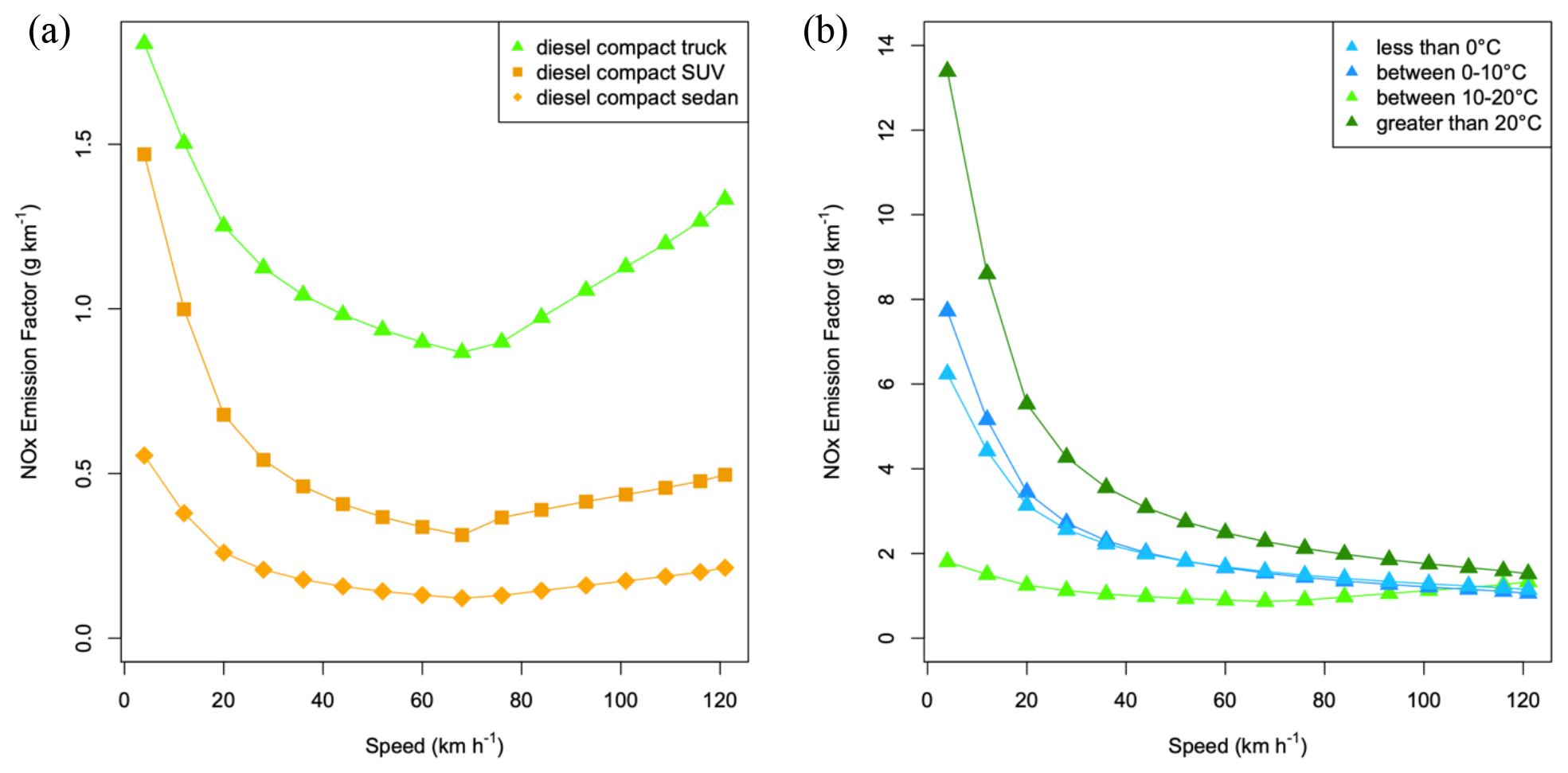
Figure 3Variation of NOx emission factors from diesel compact engines by vehicle speed and ambient temperatures: (a) NOx emission factors in relation to vehicle speed and (b) NOx emission factors of diesel compact trucks in relation to both vehicle speed and ambient temperature.
The hot exhaust emission factor, EF (g km−1), is a function of vehicle speed (spd) with other empirical coefficients: . The emission factor formula and those coefficients were developed by NIER's CAPSS (Lee et al., 2011a). These coefficients are varied by pollutants (p), vehicle type (v), vehicle manufacture year (vyr), and vehicle speed (s). The vehicle speed affects the combustion efficiency of an ICE and impacts the emission rates and its composition from the tailpipe.
While vehicle speed plays a critical role in hot exhaust emissions from most vehicles, NOx emissions from some diesel vehicles show sensitivity to local ambient temperature and humidity due to the atmospheric moisture suppression of high combustion temperatures that both lower NOx emissions at higher humidity (Choi et al., 2017; Ntziachristos and Samaras, 2000). Figure 3 shows the dependency of NOx emission factors from compact diesel vehicles on vehicle speed (Fig. 3a) and ambient temperature (Fig. 3b). Figure 3a shows a significant decrease in NOx emissions when the speed increases between 0 and 70 km. Figure 3b demonstrates the significance of local meteorology regarding NOx emissions from a compact diesel sedan. Based on these NIER's CAPSS emission factors, the sensitivity to local ambient temperature is limited to NOx pollutant emissions from diesel vehicles.
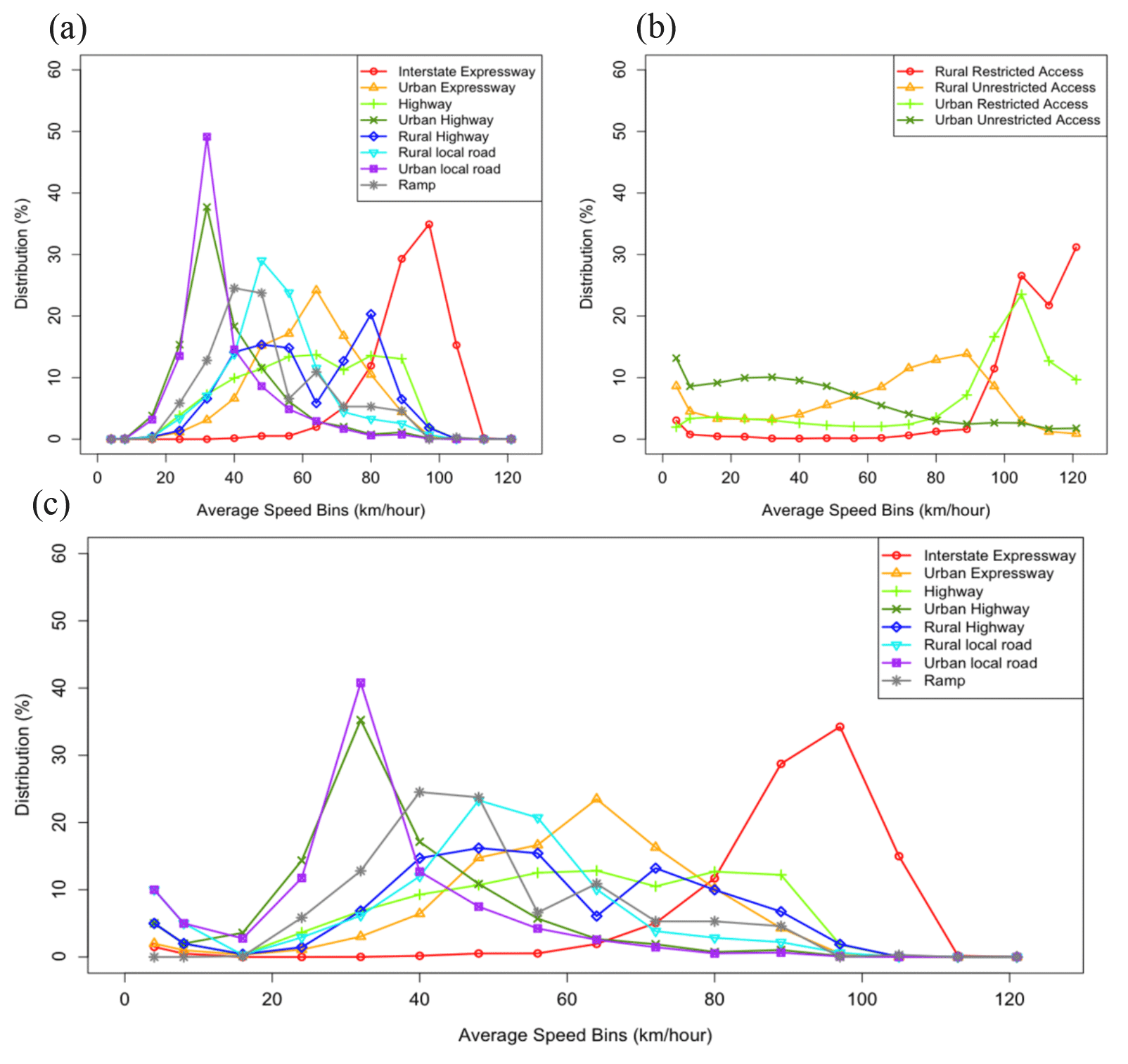
Figure 4(a) South Korean speed distribution by road type. (b) The speed distribution by road type for the state of Georgia (US). (c) The average speed distribution (ASD) by road type used in this study for South Korea.
Due to its high sensitivity to the vehicle operating speed, it is important for the CARS to simulate realistic speed patterns for accurate emissions estimates. When a single speed is assigned to compute hot exhaust emissions, it will not reflect the emissions under low-speed circumstances. To overcome this limitation, the CARS has adopted the 16 average speed bins concepts for a better representation of vehicle speed distribution that varies by road type (i.e., local, highway, expressway). We have implemented a feature for the CARS optionally to apply road-specific average speed distributions (ASDs) (Abin,r) by 16 speed bins (bin) (from 0 to 121 km h−1 defined in Appendix E) for eight different road types (r) (nos. 101–108, shown in Appendix C) as classified by CAPSS (Fig. 4a). Although ASD patterns vary by region and time, the current CARS model version does not support ASD application by region and time of day due to the lack its availability in South Korea.
We first developed the ASD (Fig. 4a) for eight different road types (nos. 101–108) in South Korea based on the latest road-link-specific average speed and the length of the link from the South Korean (SK) GIS road network shapefiles (NIER, 2018). However, the ASD based on the SK GIS road shapefiles did not capture low-speed (<16 km h−1) driving (Fig. 4a). This causes a significantly lower estimation of NOx and VOC emissions compared to the CAPSS (Appendix G). We believe the SK average speed distribution is missing low-speed driving that can occur due to traffic congestion. To address this absence of low-speed driving in the SK ASD, we incorporated data from the ASD (Fig. 4b) from the state of Georgia to the low speed ranges (speed bin nos. 1 and 2 for road types 1 to 7). We increased the total fractions of low speed bins (the 2:1 ratio of fractions of bin nos. 1 and 2) by 2 % for interstate expressways, 3 % for urban expressways, 7 % for all highways, and 15 % for all local roads. The increases in low-speed bins lowered the distributions of other higher-speed bins homogeneously due to the renormalization of fractions by road type. Figure 4c shows the renormalized hybrid ASDs of all road types based on the SK and Georgia ASDs. We understand that the hybrid ASD approach is not ideal for SK on-road emission inventory development, but it clearly demonstrates the CARS's capability and sensitivity to the vehicle speed representation.
While the application of an ASD with 16 speed bins is critical to computing more realistic hot exhaust emissions, there should be some restrictions for certain road types. Users can adjust the restricted roads control table input file to limit the vehicle types that are only operated on a particular road type. For example, motorcycles are limited on local roads (nos. 104, 106, and 107) but not on expressways (nos. 101, 102, 103, 105, and 108) due to its traffic regulation rules. Heavy trucks are only allowed on the highway (nos. 101, 102, 103, 105, and 108.) by law. The details of the road restriction control table format can be found on the CARS's user's guide from the CARS version 1 used in this paper (Baek et al., 2021).
The 16-speed-bin ASDs from Eq. (13) are added to the CARS hot exhaust emissions equation (Eq. 3). The hot exhaust emissions from individual vehicles () can be calculated by considering a road-specific speed bin distribution (Eq. 5). Although the vehicles may be operated in different districts from their registered district, this is our best method to estimate the vehicle speed for hot exhaust emissions.
2.2.2 Cold start emissions
The cold start emissions occur when a cold engine vehicle is ignited. Lower temperatures of the ICE are not optimal conditions for complete fuel combustion. This process lowers the combustion efficiency (CE) and increases the emissions of hydrocarbon and CO pollutants from the tailpipe exhaust (Lee et al., 2011). The CARS can estimate the cold start emissions for vehicles using gasoline, diesel, or liquefied petroleum gas (LPG) fuel. Besides the vehicle and engine type, road type also plays a critical role in the quantity of cold start emissions because it occurs mostly in parking lots and rarely occurs on highways.
The cold start emission, Ecold (g d−1), is derived from the hot exhaust emissions, the ratio of hot to cold exhaust emissions (EF −1.0), and the percentage of the traveled distance with a cold engine (Eq. 6).
The emission factor of cold start emissions (EFcold) is not directly calculated from measurement data like hot exhaust emissions () but measured under different ambient temperatures (T). The CARS model applies linear regression models developed by CAPSS to estimate the increasing ratio of cold start to hot exhaust emissions (EF) under different temperatures (T) (Eq. 7). In this equation, A and B are the empirical coefficients that vary by the pollutant (p) and vehicle type (v).
β is the percentage of the distance traveled under a cold engine and also depends on the ambient temperature. Cold ambient temperatures cause a longer distance traveled under a cold engine due to the slower heating time. According to the CAPSS database for the city of Seoul (Lee et al., 2011a), the empirical linear equation for β is shown in Eq. (8). This formula represents how ambient temperature affects β. For example, when the average temperature is −2 ∘C, β is 34.8 %. In summer, the monthly average temperature is 25.7 ∘C, which causes β to drop to 21 %.
2.2.3 Evaporative VOC emissions
Evaporative emissions are emissions from vehicle fuel that are evaporated into the atmosphere. This occurs in the fueling system inside the vehicle, such as fuel tanks, injection systems, and fuel lines. Diesel vehicles, however, can be exempted due to diesel fuel's low vapor pressure. The primary sources of evaporative emissions are breathing losses through tank vents and fuel permeation/leakage. The CARS model adopted the EEA's emission inventory guidebook (EEA, 2019) to account for diurnal emissions from the tank (ed), hot and warm soak emissions by fuel injection type (Sfi), and running loss emissions (R) (Eq. 9). Unlike CAPSS, there is a conversion factor (0.075) applied to Evap for motorcycles to prevent an overestimation of VOCs.
Diurnal emissions, ed (g d−1), during the daytime are caused by the ambient temperature increase and the expansion of fuel vapors inside the fuel tank. Most of the current fuel tank systems have emission control systems to limit this kind of evaporative VOC emissions. The ed can be calculated with the empirical Eq. (10), which was developed by CAPSS. Tl is the monthly average of the daily lowest temperatures, and Th is the monthly average of the daily highest temperatures. The empirical coefficient α is 0.2, which represents how 80 % of emissions are eliminated by the vehicle emission control system.
Soak emissions (Sfi) occur when a hot ICE is turned off; the remaining heat from the ICE can increase the fuel temperature in the system, which causes the increase of evaporative VOC emissions. This carburetor float bowls are the major source of the soak emissions. Newer vehicles with fuel injection and returnless fuel systems do not emit soak emissions. Because most of the current vehicles in South Korea have a new fuel system, soak emissions (Sfi) in the CARS model are set to 0.
The running loss emissions (Rl) are from vapors generated in the fuel tank when a vehicle is in operation (Eq. 11). In some older vehicles, the carburetor and engine operation can increase the temperature in the fuel tank and carburetor, which can cause a significant increase in evaporative VOC emissions. VOC emissions from running loss can be greatly increased during warmer weather. However, newer vehicles with fuel injection and returnless fuel systems are not affected by the ambient temperature. Because most vehicles in South Korea do not use carburetor technology, we expect running loss emissions to have the least impact (Lee et al., 2011b).
The empirical coefficient α is 0.1 here, which represents that 90 % of the running loss is avoided by the newer fuel system. L is the distance traveled (km) by road and is the same variable used in hot exhaust emission calculations. β is the same parameter from Eq. (8). The Rh and Rw are the average emission factors from running loss under hot and warm or cold conditions, respectively.
2.3 Road-link-level emissions calculations
In general, district-level automobile emissions calculations are driven by district-level averaged vehicle activity and operating data, which do not reflect realistic spatial patterns of on-road automobile emissions. The CARS model introduces road-link-specific traffic data by default to develop spatially enhanced road-link-specific emissions that are more representative of the emissions. This high-resolution traffic data is a GIS shapefile that is composed of many connected segments, which are called “road links”. All road links hold information such as start and end location coordinates, AADT, road link length, averaged vehicle speed, and road type (nos. 101–108).
The CARS model applies link-level AADT (AADT, d−1) and road length () to compute the road-link-specific VKT (VKT, km d−1) in Eq. (12). The road links are identified by district (dst), road type (r), and link (l) labels. The road VKT is a parameter that reflects the traffic activity of each road link and it is different from individual daily vehicle activity data (VKTv,age) in Eq. (1).
Road-link-specific VKT (VKT) is used to redistribute the district total emissions (Eonroad) from Eq. (2) into road-link-level emissions. The following three weight factors are computed: the district weight factors, ωdst (Eq. 13), the road type weight factors, ωdst,r (Eq. 14), and the road link weight factors, ωdst,l (Eq. 15). The weight district factors (ωdst) are the renormalization of each district's total VKT over state-level total VKT (N is the number of districts). The main reason we performed the renormalization over state-level total VKT is to reflect daily traffic patterns from multiple districts under the assumption that most vehicles travel within the same state. The road type weight factors by district (ωr,dst) are used to compute road-specific emissions, while road-specific averaged speed distributions (ASD; Aspd,r) from Eq. (5) are applied to capture vehicle operating speeds by road type. The road link weight factors (ωdst,l) are then applied to redistribute the district emissions into road-link-level emissions.
The CARS model is an open-source program based on Python (Van and Drake, 2009) that allows users to efficiently apply open-source modules to develop programs. Users can easily install Python development tools and load customized packages and modules to set up the CARS development environment. All CARS modules are developed using Python v3.6. Other than the GIS road shapefiles, all input files are based in the ASCII CSV format, which can be easily handled by both spreadsheet programs and programming languages, making it more accessible for users of all skill sets. The CARS is not only able to estimate district-level and spatially enhanced road-link-level emissions but is also able to generate hourly chemically speciated gridded emissions for CTMs. In addition, the CARS also generates various summary reports, graphics, and georeferenced plots for quality assurance.
The required Python modules for the CARS are “geopandas”, “shapely.geometry”, and “csv” modules to read the shapefiles and table data files. The “NumPy” and “pandas” modules are used to operate the memory arrays and scientific calculations, while the “pyproj” module deals with converting the projection coordinate systems. The “matplotlib” module is for generating any type of figures and plots. Furthermore, the CARS model can also read and write Climate and Forecast (CF)-compliant NetCDF-formatted files using “NetCDF4”.

The first process in the CARS is “Loading_function_path”, which allows users to define and check the input file paths. Once all input files are checked, there are six process modules in CARS to process inputs, compute emissions, and generate various output files, including QA reports. Figure 5 is the schematic of the CARS that consists of six process modules with various functions. The six process modules are (1) “process activity data”, (2) “process emission factors”, (3) “process shapefile”, (4) “calculate district emissions”, (5) “Grid4AQM”, and (6) “plot figures”. The main purpose of modularizing the CARS is to meet the needs of various communities, such as policymakers, stakeholders, and air quality modelers. While modules (1) through (4) are required to develop the district-level and road-link-level emissions inventories, module (5) is optional depending on whether users want to develop chemically speciated gridded hourly emissions for CTMs. In addition, the modularity of the CARS allows users to bypass certain modules if it has been previously processed without any changes. For example, if there is no change in traffic activity, emission factors table, or GIS shapefiles, users do not need to run these modules and can simply read the data frame outputs and then run Grid4AQM for the modeling dates and domain. The Grid4AQM module will not only improve the computational time for CTMs but also eliminate the need for a third-party emissions modeling system like SMOKE (Baek and Seppanen, 2021).
The rectangular boxes in Fig. 5 represent the data array and the boxes with rounded edges are the functions in the CARS. Details on the CARS code, input table format, and function setup information can be found on the CARS GitHub website (Pedruzzi et al., 2020).
The process activity data module first reads the vehicle activity data, such as an individual vehicle's daily total VKT based on its registered district. The process emission factors module reads and stores the emission factors table that holds all pollutant emission factors to estimate the emissions for all vehicles. Meteorology-sensitive emission factors are only limited to NOx pollutants. District boundary GIS shapefiles and road network shapefiles are processed through the process shape file module to generate the VKT-based redistribution weighting factors from Eqs. (13), (14), and (15) for the calculate district emissions module to compute district-level and road-link-level emission rates (metric tons per year, t yr−1).
The redistributed emission rates (t yr−1) from the calculate district emissions module present annual total emission rates until district-level VKTs from the process activity data module are added. Following this, the Grid4AQM module can generate CTM-ready chemically speciated emissions. The “read_chemical” function from the Grid4AQM module is designed to process the chemical speciation profile that can convert the inventory pollutants, such as CO, NOX, SO2, PM10, PM2.5, VOCs, and NH3, into the chemically lumped model species that CTM requires for chemical mechanisms, such as Statewide Air Pollution Research Center (SAPRC) chemical mechanism (Carter and Heo, 2013) and Carbon Bond version 6 (CB6) (Yarwood and Jung, 2010). The “read_temporal” function processes the complete set of monthly, weekly, and hourly temporal allocation profiles that can convert annual total emissions to hourly emissions. The “read_griddesc” function defines the CTM-ready modeling domain and computes the gridding fractions for all road-link-level emissions by overlaying the modeling domain over the GIS shapefiles. Once annual total emissions are chemically speciated, spatially gridded, and temporally allocated into hourly emissions, the “gridded_emis” function will combine emission source-level conversion fractions from each function (read_chemical, read_temporal, and read_griddesc) to generate the CTM-ready chemically speciated, gridded hourly emissions in the NetCDF binary format. The plot figures module is designed for generating various summary reports and graphics to assist users in understanding the estimated automobile emissions inventory computed by the CARS. The following section will describe the detailed processes of the Grid4AQM module, which includes chemical, spatial, and temporal allocations.
The influence of temperature on emission processes is considered in the CARS model. There are three temperature parameters in current CARS model: “temp_max” for maximum temperature, “temp_mean” for mean temperature, and “temp_min” for minimum temperature. These temperature parameters will be applied over the entire modeling domain during the simulation period. The current CARS model version does not yet support to process gridded meteorology data from third-party meteorology models like the Meteorology–Chemistry Interface Processor (MCIP) from the U.S. EPA and the Weather Research Forecasting (WRF) model from the National Center for Atmospheric Research (NCAR). However, CARS can easily adopt various temporally resolved temperature values by adjusting the CARS simulation period (i.e., day, week, month, season, or year).
3.1 Chemical speciation
To support CTM applications, the CARS needs to be able to convert inventory pollutants into chemical lumped model species based on the choice of CTM chemical mechanisms. NOx includes nitric oxide (NO), nitrogen dioxide (NO2), and nitrous acid (HONO). VOCs can represent hundreds of different organic carbon species, such as benzene, acetaldehyde, and formaldehyde. These grouped inventory pollutants cannot be directly imported into the chemical mechanism modules in the CTM system and require chemical speciation allocation for CTMs to process them during their chemical reactions. Therefore, the Grid4AQM module performs the chemical species allocation step prior to the temporal and spatial allocations to generate the gridded hourly emissions. The read_chemical function in the Grid4AQM module allows users to assign these emission inventory pollutants to CTM-ready surrogate chemical species (i.e., lumped chemical species) by vehicle, engine, and fuel type. For example, VOC emissions from diesel buses can be converted into the following composition based on its chemical allocation profile when the CB6 chemical mechanism is selected: alkanes (68 %), toluene (9 %), xylenes (8 %), alkenes (4 %), ethylene (2 %), benzene (1.3 %), and unreactive compounds (7 %). Further details on the chemical speciation profile input formats are available in the CARS user's guide.
3.2 Spatial allocation
The calculate district emissions module calculates both total district and road link specific emissions based on road-link-specific AADT data from road network GIS shapefiles. The calculate district emissions module first gets the district total vehicle emissions (Eq. 2) based on the district-level VKTs and then the normalized district total emissions by district weight factor, ωd (Eq. 13). Afterwards, the normalized district total emissions are redistributed into every road link using road-link-level weight factors (ωd,l) (Eq. 15). The district total emissions from Eq. (2) and Eq. (15) remain the same. Thus, the computed road-link-level emissions will then be converted into grid cell emissions using the modeling domain grid cell fractions computed in the Read_griddesc function in the Grid4AQM module.
3.3 Temporal allocation
Once chemical and spatial allocations are completed, the final step to support CTM application is a temporal allocation that converts the annual total emissions from the calculate district emissions module into hourly emissions. The Read_temporal temporal allocation function in the Grid4AQM module converts the annual emission rate (t yr−1) to the hourly emission rate (mol h−1) using monthly, weekly, and weekday–weekend diurnal temporal profiles. This module processes these temporal profile inputs, which are the monthly (January–December), weekly (Monday–Sunday), and weekday–weekend 24 h profile tables (00:00–23:00 LT, local time). The users can assign these temporal profiles with a combination of vehicle, engine, fuel, and road types to enhance their temporal representations in detail.
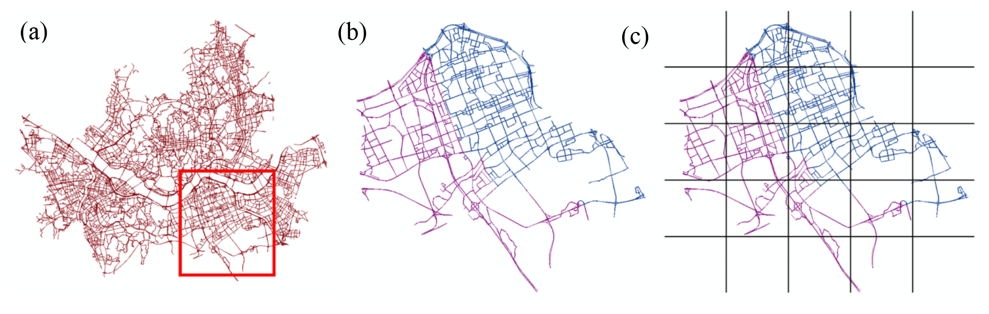
Figure 6(a) The road network GIS shapefile of Seoul, South Korea. (b) Two districts differentiated using different colors (purple and blue). (c) The modeling grid cells shown over the road segments.
3.4 Chemical transport model emissions
The main goal of the Grid4AQM module is to generate temporally, chemically, and spatially enhanced CTM-ready gridded hourly emissions. First, it reads the CTM modeling domain configuration and then overlays it over the road network GIS shapefile and district boundary shapefile to define the modeling domain. This overlaying process between the road network, district boundary GIS shapefiles, and modeling domain allows the Grid4AQM module to compute the fraction of road links that intersects with each grid cell. Figure 6 demonstrates how the district boundary and road network GIS shapefiles are used to perform the spatial allocation processes in CARS. Figure 6a is a native road link shapefile of Seoul with AADT, VKT, district ID, and road type. Figure 6b presents an overlay of two districts' road links (purple and blue) over the selected region. State total emissions will be renormalized into weighed district total emission data and then redistributed into the road link. Figure 6c illustrates how the weighted road-link-level emissions get allocated into modeling grid cells for CTMs. The link-level VKT (VKT) from Eq. (12) will be used to compute a total of traffic activity fractions by grid cell and then use that to assign the link-level emissions from Eq. (2) into each grid cell. When a road link intersects with multiple grid cells, the “Grid4AQM” module will weigh the emissions by the length of the link that intersects with each grid cell. It should be noted that current CARS model can only generate the Community Multiscale Air Quality (CAMQ)-ready gridded hourly emissions in the IOAPI (Input/Output Applications Programming Interface) format, which is based on the NetCDF format.
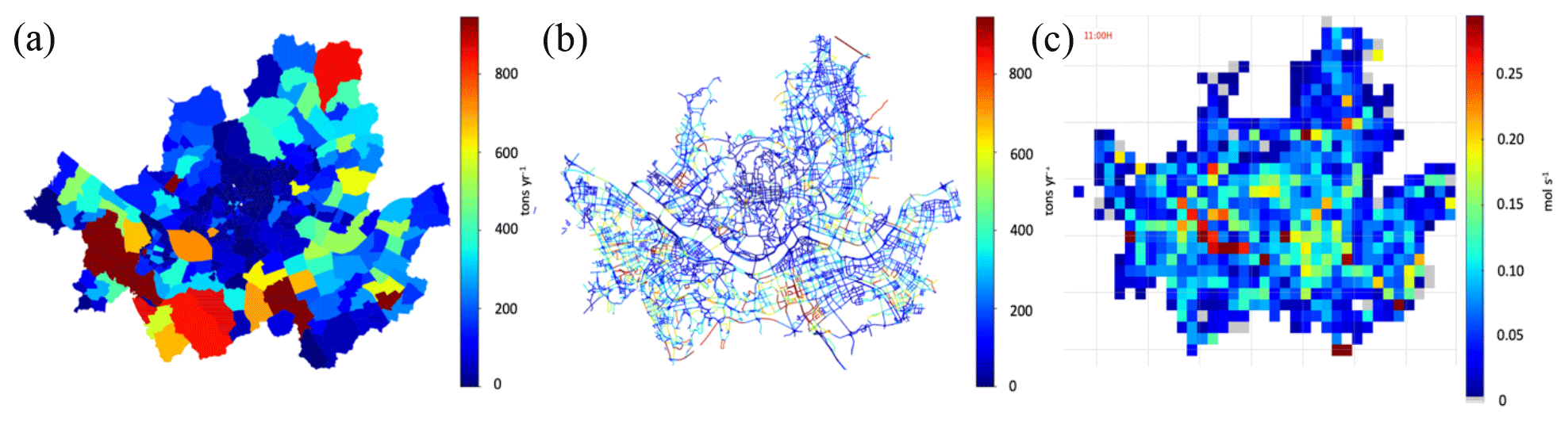
Figure 7Three different formats of CO emissions from CARS: (a) district-level total emissions (t yr−1), (b) link-level total emissions (t yr−1), (c) and CTM-ready gridded hourly total emissions (mol s−1).
Through the overlay process, the CARS model can generate various types of output data, such as total district emissions, link-level emissions, and CTM-ready gridded emissions. For example, the CO vehicle emissions from the Seoul metropolitan area in South Korea are presented in three different output formats in Fig. 7. Figure 7a shows the annual mobile PM2.5 emissions by district. The road link level annual emissions are presented in Fig. 7b. Furthermore, the CARS applies the link-level emissions from Fig. 7b to generate the hourly grid cell emission data with a 1 km×1 km resolution for the CTM in Fig. 7c.
3.5 National control strategy application
One of the unique features in the CARS compared to other mobile emissions models is that it can promptly develop a strategy to control automobile emissions in response to national emergency high PM2.5 episodes. It is very common to experience high PM2.5 episodes, especially during the wintertime in South Korea due to domestic and international primary and secondary air pollutants emissions. When the 72 h forecasted PM2.5 concentration exceeds the average. 50 µg m−3 (00:00–16:00 LT), the national PM2.5 emergency control strategy is activated for 10 d. It applies a nationwide vehicle restriction policy within 24 h. It enforces a limit on what kind of vehicles can be operated on a certain date. The restrictions can be closures of public parks and government facilities and of certain vehicles based on their fuel type and age, which is a major factor of engine deterioration. This policy will limit the number of vehicles on the network roads significantly, which could reduce primary PM2.5 and precursor pollutant (NOx, NH3, and VOCs) emissions, especially from heavily populated metropolitan regions (Choi et al., 2014; Kim et al., 2017a, b, c).
To understand the impacts of an even or odd vehicle number restriction policy in real time, we need to quickly develop a rapid controlled response to emissions for the air quality forecast modeling system based on the reduced number of vehicles on the road. The process of generating the controlled mobile emission inventory can take a long time if we start fresh. Thus, we have implemented this control strategy as an optional “control factors” function in the calculate district emissions in the module for users to quickly and easily generate the controlled mobile emission inventory with consideration of the limited number of vehicles based on the vehicle, engine, fuel, and vehicle manufacture year. A 100 % control factor means that there are no emissions from those selected vehicles.
Because of the modularization system in the CARS, we can bypass some computationally expensive data processing modules (i.e., process activity data, process emission factors, and process shape file) and let the calculate district emissions module quickly apply control factors while it computes the district-level mobile emission inventory from Eq. (2). This will allow users to reduce the computational time to generate the controlled mobile emissions under a specific control scenario and develop the controlled CTM-ready gridded hourly emissions using the Grid4AQM module.
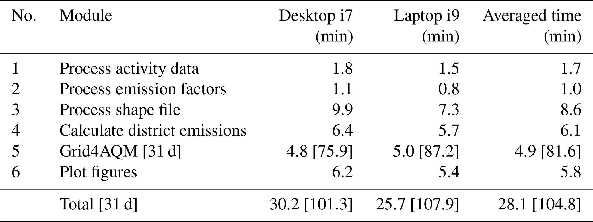
Table 1Computational processing time by CARS module based on the modeling setup. The total number of activity data is 24 383 578, there are 84 608 emission factors, there are 385 795 GIS road links, there are 5150 districts and 16 states; there are 5494 total 9 km×9 km grid cells (82 columns ×67 columns). The numbers in parentheses beside the Grid4AQM module is the computational time for 31 d (as opposed to a single day).
3.6 Computational time
While the CARS can generate a high-quality spatiotemporal emission inventory, it is quite critical for the CARS to generate them effectively and accurately without being at the expense of computational time. This is especially important to meet the needs for an air quality forecast modeling system responding to a national emergency control strategy implementation.
In this section, we will discuss the details of the CARS computational modeling performance. While the CARS model has been highly optimized, the modularization of CARS has also improved its modeling performance with its optional module runs. The breakdown of module-specific computational time estimates based on the benchmark CARS runs are listed in Table 1. The benchmark CARS case includes a total of 24 383 578 daily VKT datasets from KTSA over 2 different years, 84 608 emission factors for all pollutants across a combination of vehicle age and engine and fuel types, 385 795 road links from the GIS road network shapefiles, a 5150-district and 16-state boundary GIS shapefile, and 5494 grid cells (82 rows and 67 columns) for CTMs. Without any computational parallelization, the total processing time of all six modules usually takes around half an hour to generate a single-day CTM-ready gridded hourly emission file. However, it can be further shortened to 25–30 min on a higher-performance computer. Because of the modular system implemented in the CARS, generating 1 month (31 d) of gridded hourly emissions from CTMs takes 100 min on high-performance computers. The maximum usage of RAM can reach up to 11 GB. Table 1 shows the breakdown of computational time by each module from two different hardware setups (desktop and laptop computers). The numbers in parentheses beside the Grid4AQM module is the computational time for 31 d. While the Grid4AQM module takes an average of 4.9 min for the generation of a single day of emissions, processing a 31 d consecutively saves 46 % more time, decreasing it from 151.9 min (=4.9 min d−1 ×31 d) to 81.6 min.
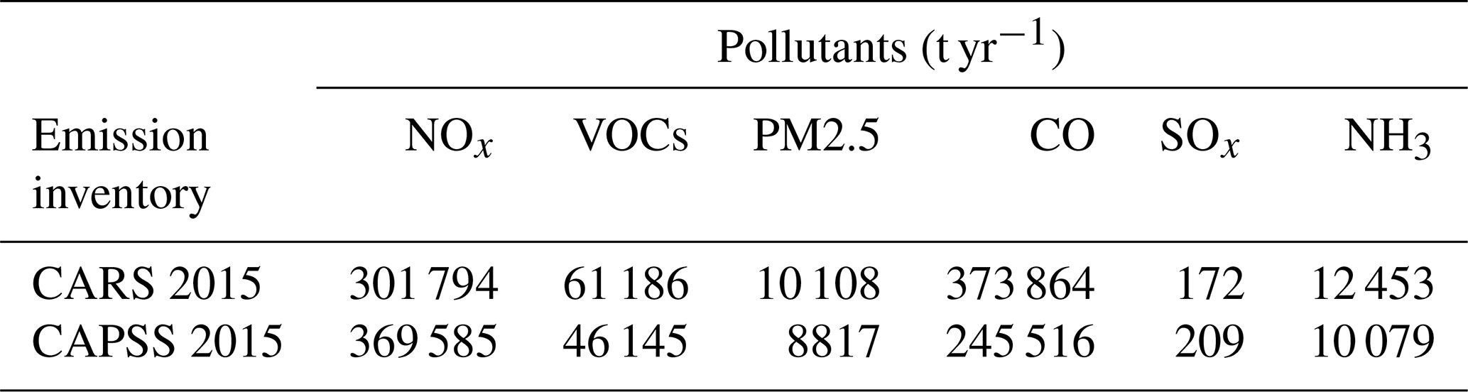
Table 2The total emissions comparison between CARS and CAPSS for 2015 emissions.
4.1 CARS and CAPSS Comparison
The CARS model calculates the 2015 on-road automobile emissions based on the latest 2015 emission factors and the 2015–2017 vehicle activity database in South Korea. The annual total emissions from CARS are compared against the ones from NIER's CAPSS in Table 2. The CARS model estimated the following annual total emissions in units of metric tons per year (t yr−1): NOx (301 794), VOCs (61 186), CO (373 864), NH3 (12 453), PM2.5 (10 108), and SOx (172.0). Compared to NIER's CAPSS, the CARS underestimated NOx (−18 % decrease) and SOx (−17 % decrease) and overestimated the emissions of VOCs by 33 %, PM2.5 by 15 %, CO by 52 %, and NH3 by 24 %. Both NIER's CAPSS and CARS shared the same emission factor tables, which hold over 84 608 emission factors for all pollutants across a combination of vehicle, age, engine, and fuel types.
The difference in results between CAPSS and CARS are caused by the three following reasons. First, the number of vehicles used in CARS is slightly higher (6 %) than CAPSS data (1.3 out of 23 million), as well as other key traffic-related activity inputs (i.e., vehicle age distribution, averaged speed distribution, etc). Secondly, the vehicle speed information assigned by vehicle and road type play a critical role. The CAPSS calculation was based on the road-specific a single average speed value or 80 % of the speed limit of the road as an input of vehicle operating speed for three road types (rural, urban, and expressway) (Lee et al., 2011b). In other words, CAPSS only assigns a “single-speed value” for each road type and does not encounter the variation of vehicle speed during its operation on roads into the emissions calculation. Most running exhaust emissions occur during a vehicle's low-speed operation due to its incomplete combustion of fuel, and it is critical to accurately represent the emissions across various speed bins in order to compute the accurate emissions (Fig. 4). A detailed analysis of the impact of vehicle speed will be discussed later in this chapter. Lastly, other advanced processes in the CARS, such as link-level AADT and district-level vehicle data (5150 districts in South Korea), can reflect more spatial detail and variation than the CAPSS. The CAPSS only considers state-level data (17 states in South Korea) and five road types (interstate expressway, urban highway, rural highway, urban local, and rural local).
Table 3Summary table of emissions (t yr−1), contributions (%) and impact factors (IFs, kg yr−1) per vehicle for criteria air pollutants (CAPs) by vehicle and fuel type (a) for NOx, (b) VOCs, (c) PM2.5, (d) CO, (e) SOx, and (f) NH3. The bold font indicates the major contributors to vehicle type and fuel type.
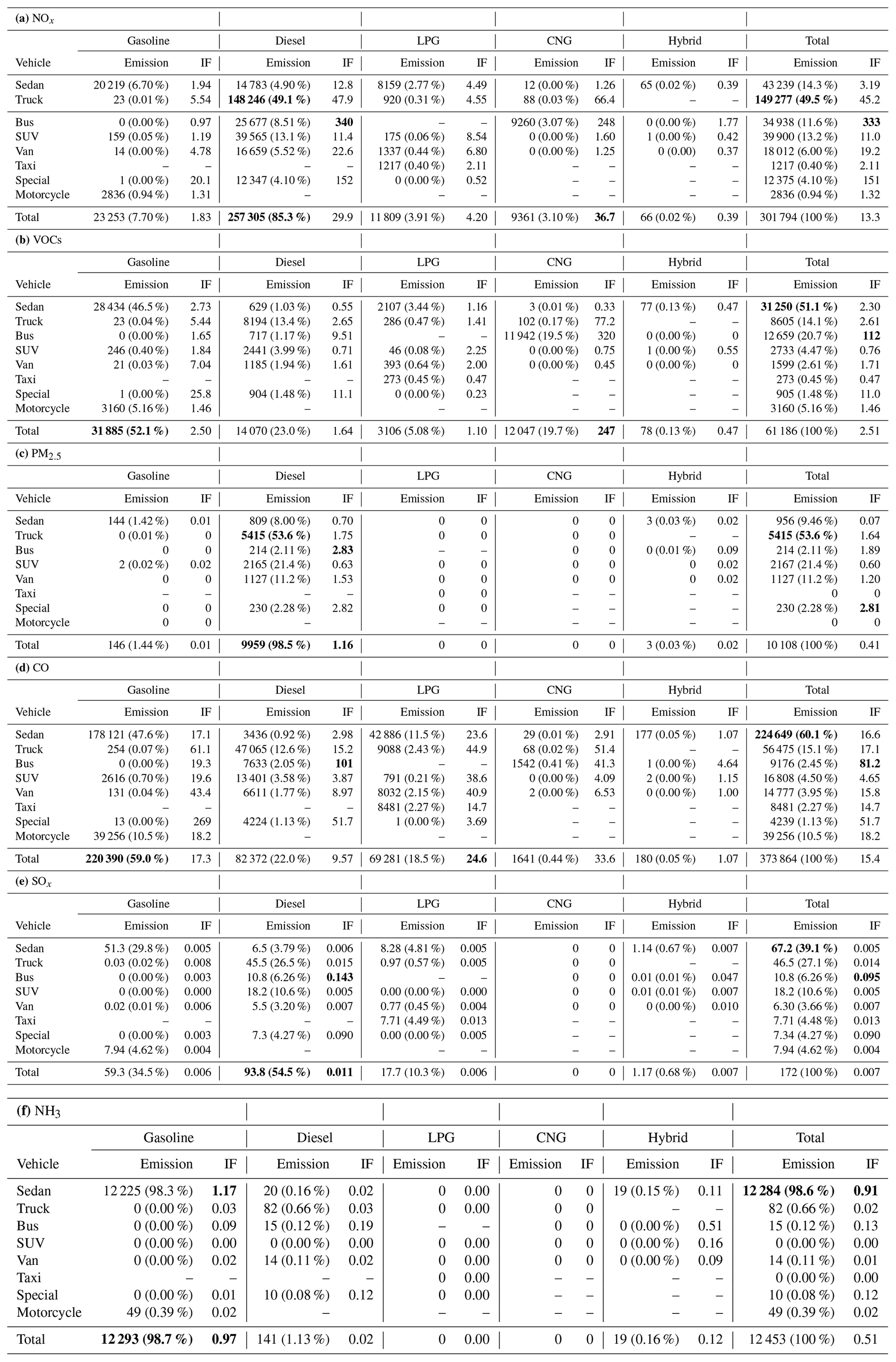
Figure 8 illustrates more details about the difference in annual emissions between CARS and CAPSS by pollutant and vehicle types. Sedan vehicles show the largest increase in VOCs (33 %), CO (41 %), and NH3 (23 %) in the CARS relative to CAPSS because almost 56 % of total vehicle count (13.5 million) is composed of sedan vehicles (Appendix B). In Table 3, sedan vehicles contribute 51 % of total VOCs and 61 % of total CO annual emissions. The VOC and CO emissions from sedans are largely affected by the average speed distribution process when compared to other vehicle types. Similarly, the largest decreases of NOx (−16 %) and SOx (−18 %) are from trucks because they are significant NOx (∼50 %) and SOx contributors (∼27 %) and their emission factors are sensitive to vehicle speed.
4.2 On-road emissions analysis
The CARS is a bottom-up emissions model that utilizes local individual vehicle activity data, detailed local emission factors for every vehicle and fuel type, and localized inputs such as average speed distribution by road type and deterioration factor. It allows users to assess a detailed breakdown of localized emission contributions. Table 3 represents the individual air pollutants (NOx, VOCs, PM2.5, CO, NH3, and SOx) emission contributions (t yr−1), fractions (%), and impact factors (IFs) by vehicle type and fuel system. The IF is defined by the normalized annual emissions with vehicle counts of each category (kg yr−1 per vehicle). The CARS also can provide the average daily VKT per vehicle, which is the total daily VKT divided by vehicle numbers, to explain the emission contributions in Appendix D.
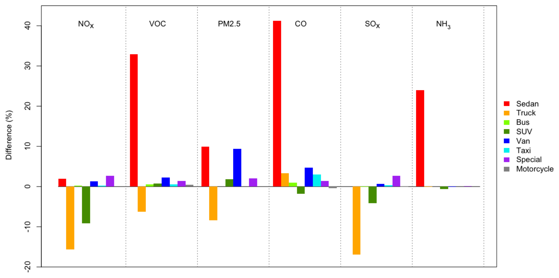
Figure 8Comparison between CARS 2015 and CAPSS 2015 on-road mobile emissions inventories by vehicle type. The standard line is CAPSS 2015 data.
Diesel-fueled vehicles contribute the most NOx emissions at over 85.3 % (257 305 t yr−1), although the number of diesel vehicles only amounts to approximately 35 % of the total vehicles (Table 3a). While diesel trucks emitted 49.1 % (148 246 t yr−1) of total NOx with an IF value of 47.9 (kg yr−1), the highest impact (IF =340 kg yr−1) occurred from diesel buses with only an 8.51 % contribution to the total NOx emissions. This is caused by the highest average daily VKT from diesel buses compared to other vehicles, which is expected in a highly populated metropolitan area like Seoul, South Korea. A diesel bus generally has a 3–5 times higher daily VKT (180 km d−1) than other common vehicles (gasoline sedan: 34 km d−1; diesel truck: 57 km d−1). The second-largest vehicle type is the compressed natural gas (CNG) bus (248 kg yr−1), which also has a high VKT at a daily average of 212 km d−1 with only a 3.1 % NOx contribution.
For VOC emissions, over 12 million gasoline vehicles cause 52.1 % (31 885 t yr−1) of the total VOC emissions, with the gasoline sedan as the highest contributor (46.5 % at 14 070 t yr−1) across all vehicle types (Table 3b). Diesel vehicles only contribute 23.0 % (14 070 t yr−1) of the total VOC emissions. The IF values from VOC indicate that CNG buses have the highest, which is 247 kg yr−1 (19 % over total VOC) with a low number of heavy CNG vehicles. The IF of the CNG bus is the highest, which is 320 kg yr−1 and emits 19.5 % of the total VOC. Comparing the IFs of buses across fuel types, the CNG bus emits less NOx but more VOCs than a diesel vehicle. Each CNG bus has about 33 times higher IF of VOCs (320 kg yr−1) than a diesel bus (9.51 kg yr−1), and CNG buses release slightly lower NOx (248 kg yr−1) than diesel buses (340 kg yr−1) (Table 3a and b).
The South Korean NIER does not currently have the PM emission factors from tire and brake wear, which are the highest contributors of PM2.5 emissions from on-road vehicles (Denier van der Gon et al., 2013; Fulvio et al., 2014). Once the emission factors of tire and brake wear are prepared, those emissions can be computed by CARS. For that reason, diesel vehicles become the major source of PM2.5 emissions, which contributes over 98.5 % (9959 t yr−1) of the PM2.5 emissions based on the CARS 2015 emissions (Table 3c). The diesel truck, SUV, and van categories are the three major sources of total PM2.5 at 53.6 %, 21.4 %, and 11.2 %, respectively. Although over 52 % of the vehicles are gasoline vehicles, their primary PM2.5 contribution is limited to 1.44 %. The diesel bus has the highest IF (2.83 kg yr−1), which is caused by the largest average daily VKTs.

Figure 9The impacts of emissions between the ASD and single-speed approach: (a) the total emission differences by pollutant and (b) the road-specific difference (%) by pollutant.
Similar to VOC emissions, CO is mostly emitted through the tailpipe due to incomplete internal combustion of fuel and shares similar emissions distributions across vehicle and fuel types (Table 3d). Gasoline vehicles contribute most of the CO (220 390 t yr−1, 59.0 %), and sedan vehicles are the primary source (178 121 t yr−1, 47.6 %) of CO out of all gasoline vehicles. Across vehicle types, buses show the highest IF of CO (81.2 kg yr−1) due to its largest daily VKT. CO is the most abundant pollutant released from vehicles (373 864 t yr−1) across all pollutants from on-road automobile sources. Although CO is much less reactive than other vehicle VOCs (Rinke and Zetzsch, 1984; Liu and Sander, 2015), CO emissions play a critical role in generating 30 % of all hydroperoxyl radicals (HO2) and cause ozone formation in urban areas (Pfister et al., 2019). Thus, CO is also another crucial precursor to ozone formation in urban areas.
SOx emissions are related to the sulfur content within the fuel component. Diesel has the highest sulfur content of any fuels, and consequently most SOx is contributed by diesel vehicles (93.8 t yr−1, 54.5 %) (Table 3e). Within diesel vehicles, trucks provide 26.5 % of SOx (45. t yr−1). Although the SOx from sedan vehicles are slightly higher (∼3.3 %) than diesel trucks, the number of diesel trucks is only 29.6 % of the number of gasoline sedans. Thus, diesel trucks have a higher IF than gasoline sedans. Across vehicle types, buses have the highest IF (0.095 kg yr−1) of SOx, and diesel buses in particular have the largest IF at 0.143 kg yr−1.
The NH3 emissions table (Table 3f) indicates that 98.7 % of NH3 is from gasoline vehicles, whereas diesel trucks only contribute 1.13 %. The IF result also shows that the gasoline sedan has the most significant impact per vehicle (1.17 kg yr−1).
According to the vehicle activity and the CARS model results, nearly half of the total vehicles (24.3 million) are gasoline sedans (10.4 million, 42.8 %), and gasoline sedan vehicles contribute the majority of VOC and CO emissions (46.5 % and 47.6 %) but only 7.7 % of the total NOx emissions. The number of diesel vehicles is at 8.6 million (35.4 %); however, they emit about 85.3 % of the total NOx and 98.5 % of the primary PM2.5. These results indicate that the annual traffic-related automobile emissions are affected not only by the number of vehicles but also by vehicle and fuel types and the age of vehicles. Therefore, this study normalized the annual emissions by the number of vehicles to confirm the emission composition by individual vehicle types.
4.3 Average speed impact study
The CARS can also optionally apply the average speed distribution (ASD) by road type to compute more realistic mobile emissions on the road network when compared to using a current single average speed value for each road type (Appendix E). Applying the ASD will generate a better representation of actual traffic patterns from each road type. To understand the impacts of ASD application, we performed sensitivity runs between using a single speed to the ASD application (Appendix F). The ASD data was described in Fig. 4, and the road-specific average single-speed values were developed based on the weighted average method using the same ASD data. Appendix E and S6 describe the details of ASD and road-specific speed values.
Figure 9a shows the differences in total emissions between two scenarios and is organized by pollutant. The single-speed scenario largely underestimates the emissions across all pollutants compared to the ones from the ASD scenario. NOx (16 %), VOC (40 %), and CO (30 %) were especially underestimated. The difference is caused by the lack of low-speed bin (<16 km h−1) representation when a single average speed approach was used. Higher emissions are emitted while vehicles are operated with low-speed bins, which decreases the combustion efficiency of ICE and releases more pollutants.
Figure 9b shows the road-specific emissions breakdown between the ASD and single-speed approaches to display the impacts of vehicle operating speeds on on-road automobile emissions. In this figure, each color indicates the emissions percentage differences by road types. Other than NH3, the most significant discrepancies are from urban local roads, highways, and urban highways, respectively. This pattern is caused by a better presentation of low-speed conditions (<16 km h−1) in CAR simulation (Appendix C). The lower speeds cause the incomplete combustion of ICE and increase the emission rate. In addition, local urban roads, highways, and urban highways have higher road VKT contributions than rural ones, at 17 %, 18 %, and 12 %, respectively (Appendix C). A better presentation of low-speed operating vehicles from highly traveled roads (urban local, urban highway, and highway) caused these significant differences between the ASD and single-speed approaches. Although the interstate expressway has the largest VKT contribution (41 %), it also has the lowest fraction of low-speed bins (2 %). That is why the difference between the ASD and single-speed scenarios on interstate expressways is less than 1 %. In general, NH3 emission factors do not change by vehicle operating speed, and thus the ASD impact is quite minimal.
The CARS is a bottom-up automobile emissions model that utilizes the localized traffic-related activity and emission factors input datasets to generate high-quality localized emissions inventories for policymakers, stakeholders, and research community as well as temporally and spatially enhanced hourly gridded emissions for CTMs. First, the CARS model employs the daily VKTs for all registered vehicles and the emission factors function to compute district-level total daily emissions for each vehicle. To reflect realistic traffic patterns, the CARS model computes and utilizes link-level VKTs (= link length × AADT) from the road network GIS shapefiles to redistribute the original district-level total emissions into spatially enhanced road-link-level emissions. It can also optionally implement a control strategy as well as road restriction rules to improve the quality of local emission inventories and meet the needs of users.
The CARS model is a fully modularized and computationally optimized Python-based model that can effectively process a huge dataset to calculate high quality spatiotemporal county-level, road-link-level, and grid-cell-level mobile emissions. We believe that the implementation of the ASD into the CARS improves the representation of on-road automobile emissions from the road network when compared to a single speed for each road type. It additionally allows the CARS to have a better representation of low-speed (<16 km h−1) vehicle emissions. We believe that the CARS model's versatile spatiotemporal bottom-up automobile emissions and in-depth analysis feature can assist government policymakers and stakeholders to quickly develop responsive emission strategies to South Korea's national PM2.5 emergency control strategy that enforces the nationwide vehicle restriction policy within 24 h.
Table A1The vehicle types classified by fuel type, vehicle body type, and engine size. The emission factors of the diesel vehicles indicated with an asterisk (*) are dependent on the ambient temperature (T).
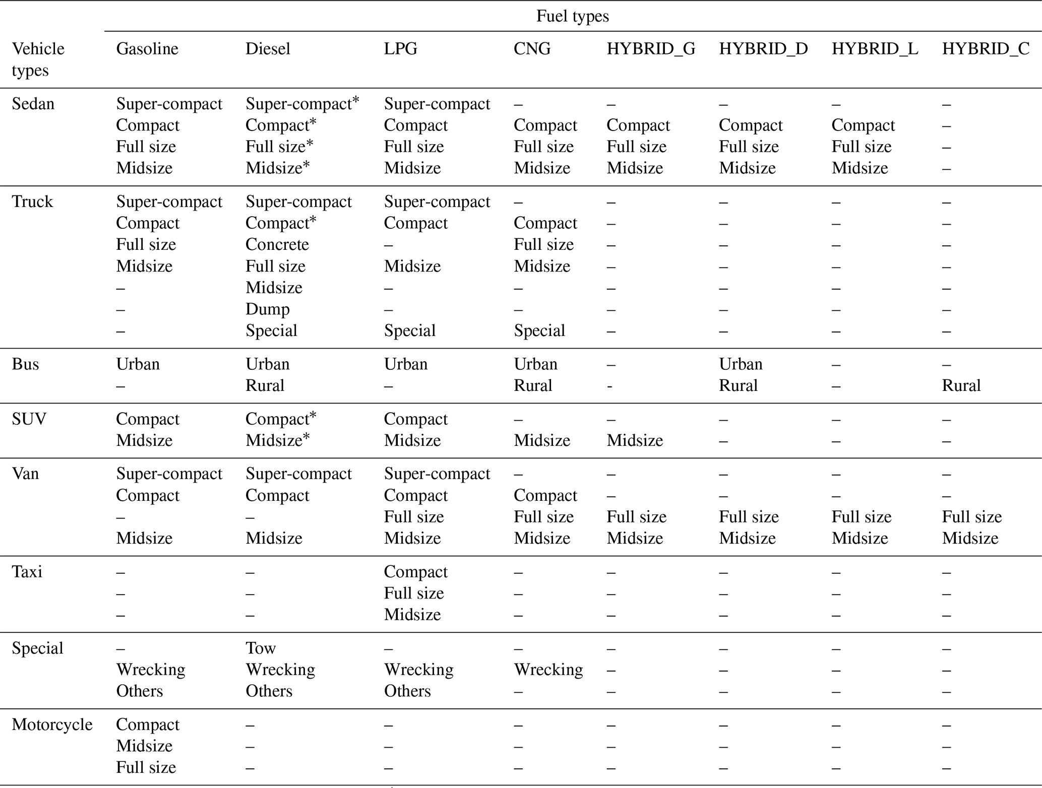
A dash indicates that the category is not applicable to the vehicle type. * Ambient-temperature-dependent diesel vehicle. LPG stands for liquefied petroleum gas. CNG stands for Connecticut natural gas. Hybrid_G stands for hybrid vehicle with gasoline. Hybrid_D stands for hybrid vehicle with diesel. Hybrid_L stands for hybrid vehicle with LPG. Hybrid_C stands for hybrid vehicle with CNG.
Table B1A summary of the activity data (number of vehicles and daily total VKTs) in South Korea by vehicle type and engine size.

A dash indicates that the category is not applicable to the vehicle type. LPG stands for liquefied petroleum gas. CNG stands for Connecticut natural gas. Hybrid is used to indicate all hybrid vehicles, i.e., electrical power mixed with fossil fuels (gasoline, diesel, LPG, or CNG).
Table C1Eight road types with assigned average vehicle operating speed and VKT fractions.
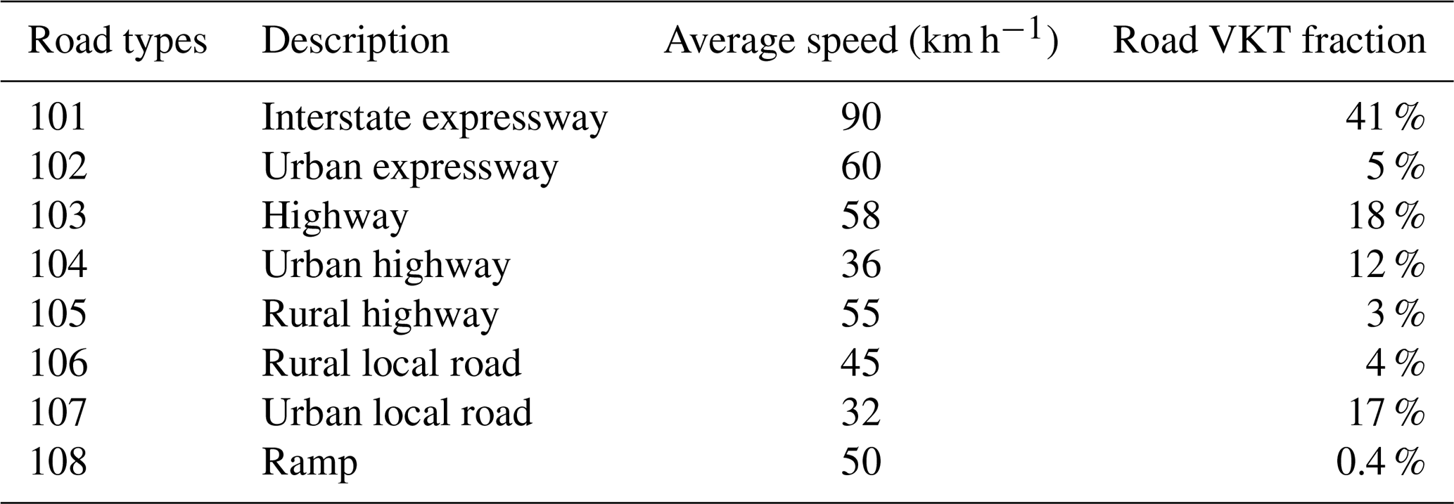
Table D1The daily average VKT (km d−1) per vehicle by vehicle and fuel type.
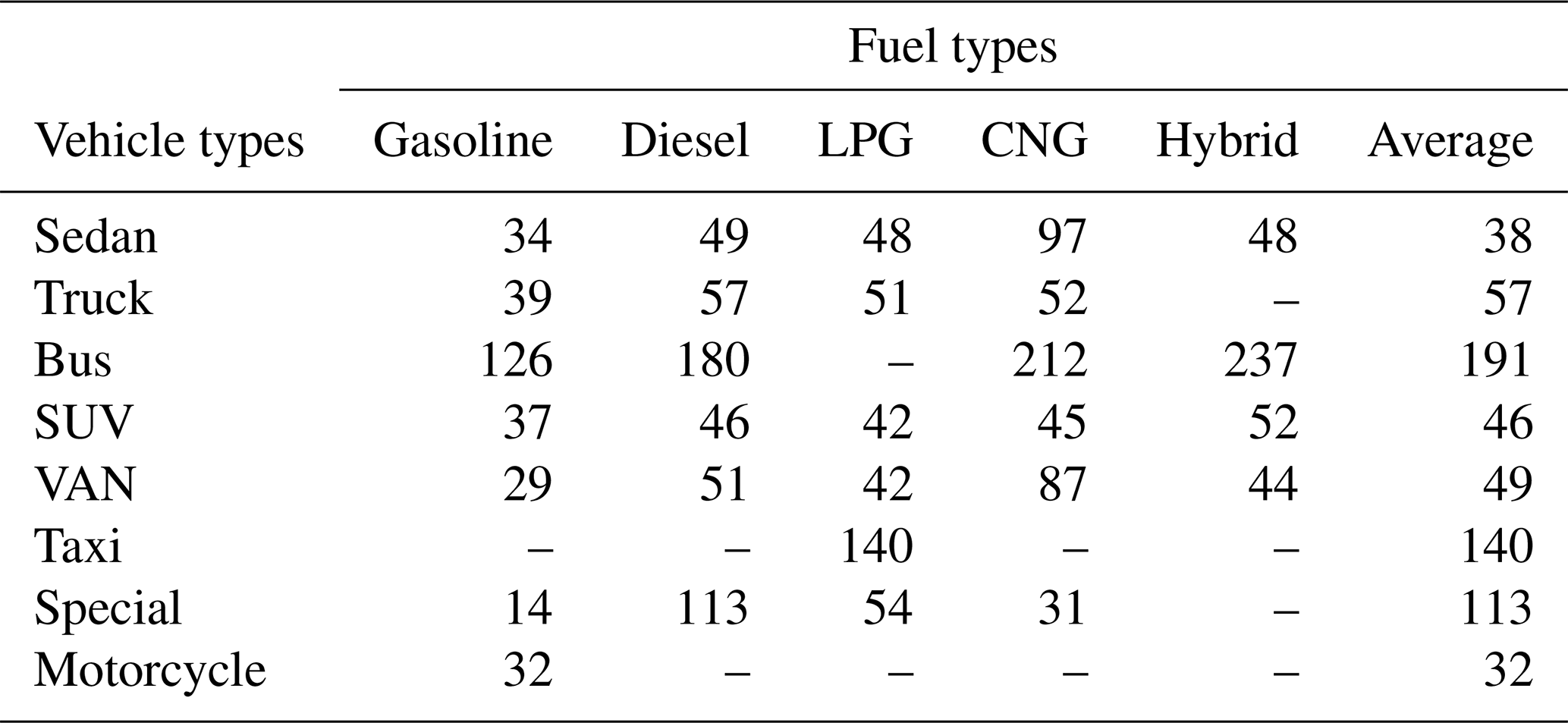
Table E1Average speed distribution (ASD) for each road type. The table columns are different road types, and the table rows are speed ranges of each speed bin.
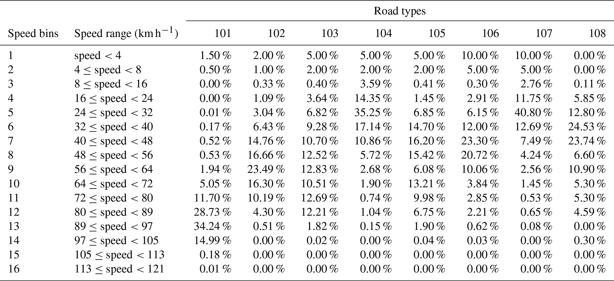
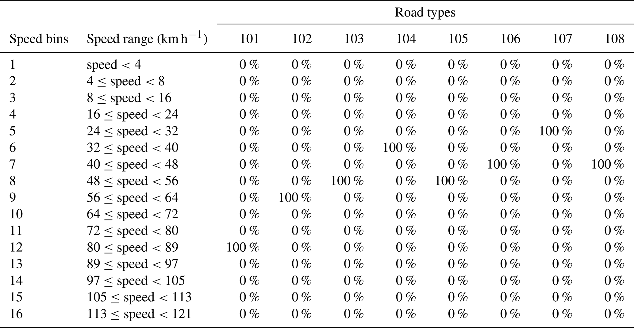
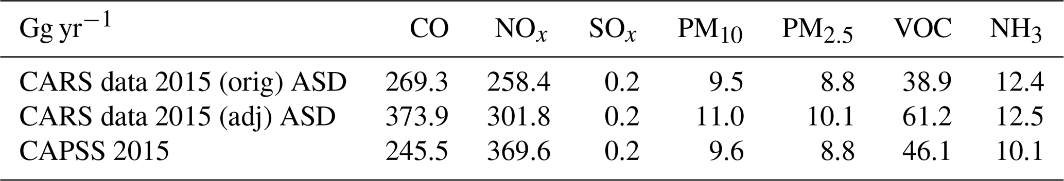
Table G1The annual emission rate between original road type ASD, adjusted road type ASD, and CAPSS result for 2015.
The source code of the CARS model public release version 1.0 can be downloaded from the GitHub release website: https://doi.org/10.5281/zenodo.5033314 (Baek et al., 2021). Digital Object Identifier (DOI) for the CARS version 1.0 is as follows: https://doi.org/10.5281/zenodo.5033314 (Baek et al., 2021). The CARS version 1.0 installation package comes with the complete input and output datasets for users to confirm the program's proper installation on their computer and can be downloaded for the CARS version 1 used in this paper (Baek et al., 2021) at https://doi.org/10.5281/zenodo.5033314 The CARS version user's guide documentation can be accessed for the CARS version 1 used in this paper (Baek et al., 2021) at https://doi.org/10.5281/zenodo.5033314 https://github.com/bokhaeng/CARS/tree/master/docs/User_Manual (last access: 18 May 2022).
All the datasets, Excel information, and Python scripts used in this paper for the data analysis have been uploaded to: https://doi.org/10.5281/zenodo.5033314 (Baek et al., 2021).
BHB and JHW are the lead researchers for this study. RP developed the source code of CARS model. MP tested the model and provided the model input data. CTW analyzed the model results and prepared the manuscript. YK and CHS also analyzed the model results and provided comments.
The contact author has declared that neither they nor their co-authors have any competing interests.
Publisher's note: Copernicus Publications remains neutral with regard to jurisdictional claims in published maps and institutional affiliations.
This research was funded by the National Strategic Project-Fine Particle of the National Research Foundation (NRF) of Korea funded by the Ministry of Science and information and communication technology (ICT) (MSIT), the Ministry of Environment (ME), the Ministry of Health and Welfare (MOHW) (NRF-2017M3D8A1092022), and the FRIEND (Fine Particle Research Initiative in East Asia Considering National Differences) Project through the National Research Foundation of Korea (NRF) funded by the Ministry of Science and ICT. (NRF-2020M3G1A1114621)
This research has been supported by the National Research Foundation of Korea (grant no. NRF-2017M3D8A1092022) and (grant no. NRF-2020M3G1A1114621).
This paper was edited by Leena Järvi and reviewed by Darrell Sonntag and one anonymous referee.
Appel, W., Chemel, C., Roselle, S., Francis, X., Hu, R.-M., Sokhi, R., Rao, S. T., and Galmarini, S.: Examination of the Community Multiscale Air Quality (CMAQ) model performance over the North American and European domains, Atmos. Environ., 53, 142–155, 10.1016/j.atmosenv.2011.11.016, 2013.
Baek, B. H. and Seppanen, C., SMOKE v4.8.1 Public Release (29 January 2021). (Version SMOKEv481_Jan2021), https://doi.org/10.5281/zenodo.4480334, 2021.
Baek, B. H., Pedruzzi, R., Wang, C.-T., and Woo, J.-H.: bokhaeng/CARS: CARS (Comprehensive Automobile Emissions Research Simulator) version 1.0 Public Release (CARSv1.0), Zenodo, https://doi.org/10.5281/zenodo.5033314, 2021.
Burnett, R., Chen, H., Szyszkowicz, M., Fann, N., Hubbell, B., Pope, C. A., Apte, J. S., Brauer, M., Cohen, A., Weichenthal, S., Coggins, J., Di, Q., Brunekreef, B., Frostad, J., Lim, S. S., Kan, H., Walker, K. D., Thurston, G. D., Hayes, R. B., Lim, C. C., Turner, M. C., Jerrett, M., Krewski, D., Gapstur, S. M., Diver, W. R., Ostro, B., Goldberg, D., Crouse, D. L., Martin, R. V., Peters, P., Pinault, L., Tjepkema, M., van Donkelaar, A., Villeneuve, P. J., Miller, A. B., Yin, P., Zhou, M., Wang, L., Janssen, N. A. H., Marra, M., Atkinson, R. W., Tsang, H., Quoc Thach, T., Cannon, J. B., Allen, R. T., Hart, J. E., Laden, F., Cesaroni, G., Forastiere, F., Weinmayr, G., Jaensch, A., Nagel, G., Concin, H., and Spadaro, J. V.: Global estimates of mortality associated with long-term exposure to outdoor fine particulate matter, P. Natl. Acad. Sci. USA, 115, 9592, 10.1073/pnas.1803222115, 2018.
Carter, W. P. L. and Heo, G.: Development of revised SAPRC aromatics mechanisms, Atmos. Environ., 77, 404–414, https://doi.org/10.1016/j.atmosenv.2013.05.021, 2013.
Choi, D., Beardsley, M., Brzezinski, D., Koupal, J., and Warila, J.: MOVES Sensitivity Analysis: The Impacts of Temperature and Humidity on Emissions, https://www3.epa.gov/ttn/chief/conference/ei19/session6/choi.pdf (last access: 18 May 2022), 2017.
Choi, K.-C., Lee, J.-J., Bae, C. H., Kim, C.-H., Kim, S., Chang, L.-S., Ban, S.-J., Lee, S.-J., Kim, J., and Woo, J.-H.: Assessment of transboundary ozone contribution toward South Korea using multiple source–receptor modeling techniques, Atmos. Environ., 92, 118–129, https://doi.org/10.1016/j.atmosenv.2014.03.055, 2014.
Cohen, A. J., Brauer, M., Burnett, R., Anderson, H. R., Frostad, J., Estep, K., Balakrishnan, K., Brunekreef, B., Dandona, L., Dandona, R., Feigin, V., Freedman, G., Hubbell, B., Jobling, A., Kan, H., Knibbs, L., Liu, Y., Martin, R., Morawska, L., Pope, C. A., III, Shin, H., Straif, K., Shaddick, G., Thomas, M., van Dingenen, R., van Donkelaar, A., Vos, T., Murray, C. J. L., and Forouzanfar, M. H.: Estimates and 25-year trends of the global burden of disease attributable to ambient air pollution: an analysis of data from the Global Burden of Diseases Study 2015, Lancet, 389, 1907–1918, https://doi.org/10.1016/S0140-6736(17)30505-6, 2017.
Denier van der Gon, H. A. C., Gerlofs-Nijland, M. E., Gehrig, R., Gustafsson, M., Janssen, N., Harrison, R. M., Hulskotte, J., Johansson, C., Jozwicka, M., Keuken, M., Krijgsheld, K., Ntziachristos, L., Riediker, M., and Cassee, F. R.: The Policy Relevance of Wear Emissions from Road Transport, Now and in the Future – An International Workshop Report and Consensus Statement, J. Air Waste Manage., 63, 136–149, https://doi.org/10.1080/10962247.2012.741055, 2013.
Dennis, R., Fox, T., Fuentes, M., Gilliland, A., Hanna, S., Hogrefe, C., Irwin, J., Rao, S. T., Scheffe, R., Schere, K., Steyn, D., and Venkatram, A.: A framework for evaluating regional-scale numerical photochemical modeling systems, Environ. Fluid. Mech., 10, 471–489, https://doi.org/10.1007/s10652-009-9163-2, 2010.
EEA: EMEP/EEO air pollutant emission inventory guidebook 2019, Passenger cars, light commercial trucks, heavy-duty vehicles including buses and motor cycles, 1.A.3.b.i-iv, European Enviromnent Agency, 2019.
Fallahshorshani, M., André, M., Bonhomme, C., and Seigneur, C.: Coupling Traffic, Pollutant Emission, Air and Water Quality Models: Technical Review and Perspectives, Proced. Soc. Behav., 48, 1794–1804, https://doi.org/10.1016/j.sbspro.2012.06.1154, 2012.
Fulvio, A., Cassee, F. R., Denier van der Gon, H. A. C., Gehrig, R., Gustafsson, M., Hafner, W., Harrison, R. M., Jozwicka, M., Kelly, F. J., Moreno, T., Prevot, A. S. H., Schaap, M., Sunyer, J., and Querol, X.: Urban air quality:The challenge of traffic non-exhaust emissions, J. Hazard. Mater., 275, 31–36, https://doi.org/10.1016/j.jhazmat.2014.04.053, 2014.
Guevara, M., Tena, C., Porquet, M., Jorba, O., and Pérez García-Pando, C.: HERMESv3, a stand-alone multi-scale atmospheric emission modelling framework – Part 1: global and regional module, Geosci. Model Dev., 12, 1885–1907, https://doi.org/10.5194/gmd-12-1885-2019, 2019.
Hogrefe, C., Rao, S. T., Kasibhatla, P., Hao, W., Sistla, G., Mathur, R., and McHenry, J.: Evaluating the performance of regional-scale photochemical modeling systems: Part II – ozone predictions, Atmos. Environ., 35, 4175–4188, https://doi.org/10.1016/S1352-2310(01)00183-2, 2001a.
Hogrefe, C., Rao, S. T., Kasibhatla, P., Kallos, G., Tremback, C. J., Hao, W., Olerud, D., Xiu, A., McHenry, J., and Alapaty, K.: Evaluating the performance of regional-scale photochemical modeling systems: Part I – meteorological predictions, Atmos. Environ., 35, 4159–4174, https://doi.org/10.1016/S1352-2310(01)00182-0, 2001b.
Ibarra-Espinosa, S., Ynoue, R., O'Sullivan, S., Pebesma, E., Andrade, M. D. F., and Osses, M.: VEIN v0.2.2: an R package for bottom–up vehicular emissions inventories, Geosci. Model Dev., 11, 2209–2229, https://doi.org/10.5194/gmd-11-2209-2018, 2018.
IEMA: Inventário de Emissões Atmosféricas do Transporte Rodoviário de Passageiros no Município de São Paulo, http://emissoes.energiaeambiente.org.br, last access: 1 May 2017.
Kaewunruen, S., Sussman, J. M., and Matsumoto, A.: Grand Challenges in Transportation and Transit Systems, Frontiers in Built Environment, 2, 1–5, https://doi.org/10.3389/fbuil.2016.00004, 2016.
Kim, B.-U., Bae, C., Kim, H. C., Kim, E., and Kim, S.: Spatially and chemically resolved source apportionment analysis: Case study of high particulate matter event, Atmos. Environ., 162, 55–70, https://doi.org/10.1016/j.atmosenv.2017.05.006, 2017a.
Kim, H. C., Kim, E., Bae, C., Cho, J. H., Kim, B.-U., and Kim, S.: Regional contributions to particulate matter concentration in the Seoul metropolitan area, South Korea: seasonal variation and sensitivity to meteorology and emissions inventory, Atmos. Chem. Phys., 17, 10315–10332, https://doi.org/10.5194/acp-17-10315-2017, 2017b.
Kim, H. C., Kim, S., Kim, B.-U., Jin, C.-S., Hong, S., Park, R., Son, S.-W., Bae, C., Bae, M., Song, C.-K., and Stein, A.: Recent increase of surface particulate matter concentrations in the Seoul Metropolitan Area, Korea, Sci. Rep.-UK, 7, 4710, https://doi.org/10.1038/s41598-017-05092-8, 2017c.
Lee, D., Lee, Y.-M., Jang, K.-W., Yoo, C., Kang, K.-H., Lee, J.-H., Jung, S.-W., Park, J.-M., Lee, S.-B., Han, J.-S., Hong, J.-H., and Lee, S.-J.: Korean National Emissions Inventory System and 2007 Air Pollutant Emissions, Asian J. Atmos. Environ., 5–4, 278–291, 2011a.
Lee, D.-G., Lee, Y.-M., Jang, K.-W., Yoo, C., Kang, K.-H., Lee, J.-H., Jung, S.-W., Park, J.-M., Lee, S.-B., Han, J.-S., Hong, J.-H., and Lee, S.-J.: Korean National Emissions Inventory System and 2007 Air Pollutant Emissions, Asian J. Atmos. Environ., 5, 278–291, https://doi.org/10.5572/ajae.2011.5.4.278, 2011b.
Lejri, D., Can, A., Schiper, N., and Leclercq, L.: Accounting for traffic speed dynamics when calculating COPERT and PHEM pollutant emissions at the urban scale, Transport. Res. D Tr. E., 63, 588–603, https://doi.org/10.1016/j.trd.2018.06.023, 2018.
Li, F., Zhuang, J., Cheng, X., Li, M., Wang, J., and Yan, Z.: Investigation and Prediction of Heavy-Duty Diesel Passenger Bus Emissions in Hainan Using a COPERT Model, Atmosphere, 10, 106, https://doi.org/10.3390/atmos10030106, 2019.
Liu, Y. and Sander, S. P.: Rate Constant for the OH + CO Reaction at Low Temperatures, J. Phys. Chem. A, 119, 10060–10066, https://doi.org/10.1021/acs.jpca.5b07220, 2015.
Luo, H., Astitha, M., Hogrefe, C., Mathur, R., and Rao, S. T.: A new method for assessing the efficacy of emission control strategies, Atmos. Environ., 199, 233–243, https://doi.org/10.1016/j.atmosenv.2018.11.010, 2019.
Lv, W., Hu, Y., Li, E., Liu, H., Pan, H., Ji, S., Hayat, T., Alsaedi, A., and Ahmad, B.: Evaluation of vehicle emission in Yunnan province from 2003 to 2015, J. Clean Prod., 207, 814–825, https://doi.org/10.1016/j.jclepro.2018.09.227, 2019.
Moussiopoulos, N., Vlachokostas, C., Tsilingiridis, G., Douros, I., Hourdakis, E., Naneris, C., and Sidiropoulos, C.: Air quality status in Greater Thessaloniki Area and the emission reductions needed for attaining the EU air quality legislation, Sci. Total Environ., 407, 1268–1285, https://doi.org/10.1016/j.scitotenv.2008.10.034, 2009.
Nagpure, A. S., Gurjar, B. R., Kumar, V., and Kumar, P.: Estimation of exhaust and non-exhaust gaseous, particulate matter and air toxics emissions from on-road vehicles in Delhi, Atmos. Environ., 127, 118–124, https://doi.org/10.1016/j.atmosenv.2015.12.026, 2016.
NIER: Study on Air Pollutant Emission Estimation Method in Transportation section(II) 11-1480523-003573-01, National Archives of Korea, https://www.archives.go.kr/next/manager/publishmentSubscriptionDetail.do?prt_seq=114054&page=1554&prt_arc_title=&prt_pub_kikwan=&prt_no (last access: 18 May 2022), 2018.
Ntziachristos, L. and Samaras, Z.: Speed-dependent representative emission factors for catalyst passenger cars and influencing parameters, Atmos. Environ., 34, 4611–4619, https://doi.org/10.1016/S1352-2310(00)00180-1, 2000.
Ntziachristos, L., Gkatzoflias, D., Kouridis, C., and Samaras, Z.: COPERT: A European Road Transport Emission Inventory Model, in: Information Technologies in Environmental Engineering, Environmental Science and Engineering, edited by: Athanasiadis, I. N., Rizzoli, A. E., Mitkas, P. A., and Gómez, J. M., Springer, Berlin, Heidelberg, https://doi.org/10.1007/978-3-540-88351-7_37, 2009.
Pedruzzi, R., Baek, B. H., and Wang, C.-T.: CARS, https://github.com/CMASCenter/CARS, last access: 1 May 2020.
Perugu, H., Ramirez, L., and DaMassa, J.: Incorporating temperature effects in California's on-road emission gridding process for air quality model inputs, Environ. Pollut., 239, 1–12, https://doi.org/10.1016/j.envpol.2018.03.094, 2018.
Pfister, G., Wang, C.-t., Barth, M., Flocke, F., Vizuete, W., and Walters, S.: Chemical Characteristics and Ozone Production in the Northern Colorado Front Range, J. Geophys. Res.-Atmos., 124, 13397–13419, https://doi.org/10.1029/2019jd030544, 2019.
Pinto, J. A., Kumar, P., Alonso, M. F., Andreão, W. L., Pedruzzi, R., dos Santos, F. S., Moreira, D. M., and Albuquerque, T. T. D. A.: Traffic data in air quality modeling: A review of key variables, improvements in results, open problems and challenges in current research, Atmos. Pollut. Res., 11, 454–468, https://doi.org/10.1016/j.apr.2019.11.018, 2020.
Rao, S. T., Galmarini, S., and Puckett, K.: Air Quality Model Evaluation International Initiative (AQMEII): Advancing the State of the Science in Regional Photochemical Modeling and Its Applications, B. Am. Meteorol. Soc., 92, 23–30, https://doi.org/10.1175/2010BAMS3069.1, 2011.
Rodriguez-Rey, D., Guevara, M., Linares, M. P., Casanovas, J., Salmerón, J., Soret, A., Jorba, O., Tena, C., and Pérez García-Pando, C.: A coupled macroscopic traffic and pollutant emission modelling system for Barcelona, Transport. Res. D Tr. E., 92, 102725, https://doi.org/10.1016/j.trd.2021.102725, 2021.
Rinke, M. and Zetzsch, C.: Rate Constants for the Reactions of OH Radicals with Aromatics: Benzene, Phenol, Aniline, and 1,2,4-Trichlorobenzene, Berichte der Bunsengesellschaft für physikalische Chemie, 88, 55–62, https://doi.org/10.1002/bbpc.19840880114, 1984.
Russell, A. and Dennis, R.: NARSTO critical review of photochemical models and modeling, Atmos. Environ., 34, 2283–2324, https://doi.org/10.1016/S1352-2310(99)00468-9, 2000.
Sallis, P., Bull, F., Burdett, P., Frank, P., Griffiths, P., Giles-Corti, P., and Stevenson, M.: Use of science to guide city planning policy and practice: How to achieve healthy and sustainable future cities, Lancet, 388, 2936–2947, https://doi.org/10.1016/S0140-6736(16)30068-X, 2016.
Smit, R., Kingston, P., Neale, D. W., Brown, M. K., Verran, B., and Nolan, T.: Monitoring on-road air quality and measuring vehicle emissions with remote sensing in an urban area, Atmos. Environ., 218, 116978, https://doi.org/10.1016/j.atmosenv.2019.116978, 2019.
Sun, W., Duan, N., Yao, R., Huang, J., and Hu, F.: Intelligent in-vehicle air quality management: a smart mobility application dealing with air pollution in the traffic, https://www.semanticscholar.org/paper/Intelligent-in-vehicle-air-quality-management-:-a-Sun-Duan/2ca548319ebb8a6aee7adb02ddf341aed6d6107f, last access: 19 May 2022, 2016.
Tominaga, Y. and Stathopoulos, T.: Ten questions concerning modeling of near-field pollutant dispersion in the built environment, Build. Environ., 105, 390–402, https://doi.org/10.1016/j.buildenv.2016.06.027, 2016.
Van, R. G. and Drake, F.: Python 3 reference manual, Scotts Valley, CA, CreateSpace, 10, 1593511, 2009.
Yarwood, G. and Jung, J.: Development, Evaluation and Testing of Version 6 of the Carbon Bond Chemical Mechanism (CB6), the 9th Annual CMAS Conference, Chapel Hill, NC, 11–13 October 2010, Chapel Hill, https://www.cmascenter.org/conference/2010/abstracts/emery_updates_carbon_2010.pdf, (last access: 19 May 2022), 2010.
- Abstract
- Introduction
- CARS emissions calculation
- CARS configuration
- Results
- Conclusions
- Appendix A
- Appendix B
- Appendix C
- Appendix D
- Appendix E
- Appendix F
- Appendix G
- Appendix H
- Code availability
- Data availability
- Author contributions
- Competing interests
- Disclaimer
- Acknowledgements
- Financial support
- Review statement
- References