Validation of turbulent heat transfer models against eddy covariance flux measurements over a seasonally ice-covered lake

In this study we analyzed turbulent heat fluxes over a seasonal ice cover on a boreal lake located in southern Finland. Eddy covariance (EC) flux measurements of sensible (H) and latent heat (LE) from four ice-on seasons between 2014 and 2019 are compared to three different bulk transfer models: one with a constant transfer coefficient and two with stability-adjusted transfer coefficients: the Lake Heat Flux Analyzer and SEA-ICE. All three models correlate well with the EC results in general while typically underestimating the magnitude and the standard deviation of the flux in comparison to the EC observations. Differences between the models are small, with the constant transfer coefficient model performing slightly better than the stability-adjusted models. Small difference in temperature and humidity between surface and air results in low correlation between models and EC. During melting periods (surface temperature T₀>0 ^∘C), the model performance for LE decreases when compared to the freezing periods (T₀<0 ^∘C), while the opposite is true for H. At low wind speed, EC shows relatively high fluxes (±20 W m⁻²) for H and LE due to non-local effects that the bulk models are not able to reproduce. The complex topography of the lake surroundings creates local violations of the Monin–Obukhov similarity theory, which helps explain this counterintuitive result. Finally, the uncertainty in the estimation of the surface temperature and humidity affects the bulk heat fluxes, especially when the differences between surface and air values are small.

1 Introduction

According to the latest satellite-based estimates, there are approximately 117 million lakes larger than 0.002 km² globally (Verpoorter et al., 2014). About 95 million of these are either above latitude 60^∘ N or below 56^∘ S. The seasonal lake ice zone extends in the Northern Hemisphere from 40 to 80^∘ N (Leppäranta, 2014), so it can safely be estimated that over 80 % of all lakes on Earth receive a seasonal ice cover. A very defining property of lakes with seasonal ice cover is that they display two starkly different states of their surface during the annual cycle. As the ice cover forms, the lake water is effectively isolated from the atmosphere, and the already low amount of shortwave radiation inherent for winter is almost completely attenuated in the snow and ice cover (Leppäranta, 2014). The snow/ice–air boundary replaces the water–air boundary, and radical changes in albedo, emissivity, surface roughness, energy balance, and gas exchange occur. Depending on the lake and the local climate, the snow–air boundary layer can be the dominating mode of exchange between the lake and the atmosphere. Thus, understanding the physics of seasonally ice-covered lakes is an important yet often overlooked aspect of understanding the behavior of lakes (Kirillin et al., 2012).

It is easy to understand why ice-covered lakes have been overlooked in the past, as most clearly observable activity on lakes happens during the open water season, but the remote nature of many of the seasonally ice-covered lakes has also made their research difficult from a practical and technical standpoint (Salonen et al., 2009). Nevertheless, while physical and biological processes in lakes slow down under the ice cover, they do not stop completely. Circulation is driven by sediment heat accumulated there during the summer, meltwater streaming from the surrounding catchment area, and solar radiation, with additional mixing produced via the breaking of internal waves promoted by changes in air pressure and wind, and although primary production is minimal, other biological processes still continue (Hampton et al., 2017) and affect especially the gas fluxes of the lake (Cortés and MacIntyre, 2020). Regardless of the season, lakes affect the climate at both regional and global scales. At the large scale, lakes affect the global climate by acting as small net sources of carbon (CO₂ and CH₄) into the atmosphere and also sequestering organic carbon into their sediments from internal biogeochemical processes and from the surrounding environment (Cole et al., 1994). At the small scale, due to their large heat storage, thermal inertia and evaporation, lakes can significantly affect local and regional weather patterns and microclimate, like rain and snowfall, temperature and cloudiness (Eerola et al., 2014; Ghanbari et al., 2009; Rouse et al., 2005). As lakes contribute significantly to the climate, understanding their surface heat balance more precisely has relevant implications, from local short-term weather and ice cover forecasting (Ghanbari et al., 2009) to long-term global circulation models, where the effect of lakes has been neglected almost completely (Subin et al., 2012).

The yearly cycle of a lake is driven by external forcing, which follows changes in the patterns of the components of the surface energy and water balance. The surface energy balance constitutes incoming and reflected solar radiation (also known as shortwave radiation), incoming and outgoing terrestrial radiation (also called longwave radiation), turbulent heat fluxes (latent and sensible heat flux) and the precipitation heat flux (Kirillin et al., 2012).

Annual changes in the solar radiation drive the changes in seasons, and during the summer it dominates the energy balance. In fall the incoming solar radiation decreases every day, and eventually enough heat will be lost through turbulent heat fluxes and outgoing terrestrial radiation to lower the temperature of the water column to the temperature of maximum density, which is +4 ^∘C for freshwater. Then, the lake mixes completely, while cooling continues. At high latitude, seasonal ice cover begins to form usually in the late fall during clear-sky and low-wind conditions associated with anticyclonal weather patterns, although frazil ice can also form in the turbulent surface layer of the lake as well. During nights in calm, cloud-free conditions there is significant loss of heat from the water through longwave radiation and freezing water can accumulate to the surface without being mixed with the warmer water below forming primary ice under which the more permanent congelation ice can form. Later during the winter snow can accumulate over the ice and freeze into solid, opaque snow ice. It insulates the lake more effectively from the solar radiation than the clear congelation ice. Melting begins when the radiation balance turns positive, and the surface absorbs more radiation. The length of ice season varies significantly depending on the local climate at the lake. Lakes in southern Finland spend less than half of the year under an ice cover, but above 65^∘ N lakes have on average a longer ice-on than ice-off season (Korhonen, 2006). Although statistics can be drawn, every winter on a lake is unique in regards to the length of the ice cover period, the layering of the ice cover, amount on snow accumulation and precipitation.

Radiative components of the energy balance are relatively simple to measure due to the passive instruments with low power consumption required to measure them, but turbulent heat transfer poses more challenges. During the last 4 decades the eddy covariance (EC) technique has become a very popular method in many fields of the environmental and geophysical sciences. It is an accurate, proven and well-established method for directly measuring vertical fluxes of heat, momentum, gases and particles over a wide variety of surface types and ecosystems (Aubinet et al., 2012). Its strong points are the ability to collect long, continuous time series in many different environmental and meteorological conditions. Although it has been extensively used over terrestrial environments, lately EC has been applied in marine and freshwater environments as well.

As the EC setup is not suited for all applications due to the technical complexity of its installation, simpler methods to compute the turbulent heat fluxes from more basic meteorological observations have been developed, with the bulk aerodynamic method and the profile method being the most popular. They originated from the need to estimate turbulent heat fluxes in situations where only basic meteorological parameters were available, like with remote-buoy-based oceanographic measurement stations with very low power available. They are also commonly used in global and regional climate models as well as in numerical weather prediction models due to their computational simplicity. For different applications (marine, land, etc.), the parameterization of the stability, aerodynamic roughness and other parameters of the model can be adjusted accordingly.

Estimating turbulent heat fluxes by the bulk aerodynamic method is simpler than measuring them with EC, as only basic meteorological measurements are required, but it inherently contains some limitations and uncertainty. Stable boundary-layer conditions and surface heterogeneity are especially troublesome, and the assumptions made in the Monin–Obukhov similarity theory (MOST) do not take into account all meteorological phenomena, like non-local effects produced by the surface heterogeneity present over small lakes surrounded by forests (Esters et al., 2021; Barskov et al., 2019).

While a few studies have reported short field campaign measurements of EC turbulent heat fluxes over seasonal ice-covered lakes (Franz et al., 2018; Barskov et al., 2019), long-term turbulent heat flux measurements have not been reported so far. In this study, we present a unique data set collected over a boreal lake in southern Finland over four ice-on seasons between 2014 and 2019. Previous studies of turbulent heat fluxes over lakes have been performed mostly in the open water season, like a northern boreal lake in Finnish Lapland (Lohila et al., 2015), a boreal lake in southern Finland (Nordbo et al., 2011) and the lake in question in this study, Lake Kuivajärvi (Mammarella et al., 2015). Ice-on lake energy balance has been studied, for example, on Lake Kilpisjärvi in northwestern Finnish Lapland (Leppäranta et al., 2017) and Lake Pääjärvi in southern Finland (Wang et al., 2005; Jakkila et al., 2009), but these experiments were done without EC equipment and estimated turbulent heat fluxes by bulk aerodynamic formulae and the profile method. EC over seasonal lake ice cover was performed over a thermokarst lake in Siberia (Franz et al., 2018), but it was also only for one winter. Thus, the data set presented here gives us a unique look at the dynamics of turbulent heat fluxes over seasonal lake ice cover as well as a possibility of validating the functionality of bulk transfer models in this environment.

2 Material and methods

2.1 Site

Lake Kuivajärvi is a dimictic, mesotrophic lake in southern Finland (long $\mathrm{24}{}^{\circ }{\mathrm{16}}^{\prime }$ E, lat $\mathrm{61}{}^{\circ }{\mathrm{50}}^{\prime }$ N; 141 m above mean sea level). It is located in the Kokemäenjoki water system, which drains into the Baltic Sea. The lake has a strongly elongated shape, 2.6 km in the north–south direction and 200–400 m in the east–west direction (Fig. 1). Due to this shape, wind is usually channeled along the lake (Mammarella et al., 2015). The lake has two basins, the southern basin being the deeper one with a maximum depth of 13.2 m. The raft used for EC and most of the meteorological measurements is located approximately over this deepest point. Lake Kuivajärvi is surrounded mostly by managed Scots pine forest, which is also the home of the SMEAR II station (Hari and Kulmala, 2005). A typical ice cover period in Lake Kuivajärvi lasts for about 5 months, starting in late November–early December and ending in late April–early May. A mild decreasing trend in the length of the ice-on season has been observed here since the start of observations in 1929 (Korhonen, 2006). The ice cover thickness at the start of the melting period is typically 40–50 cm.

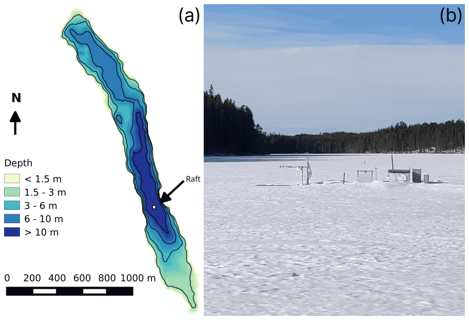
Figure 1 Bathymetric map of Lake Kuivajärvi with the position of the EC raft shown as a white square (a). Photo (b) shows the raft as it stood in March 2021. Map adapted from Erkkilä et al. (2018).

2.2 Measurement of fluxes and meteorology

Fluxes of momentum, sensible (H) and latent heat (LE) and supporting meteorological measurements were performed on a raft anchored at the deepest point of the lake as well as on the nearby SMEAR II station (Mammarella et al., 2015). The EC system consists of a Metek (Metek GmbH, Elmshorn, Germany) USA-1 three-axis anemometer providing the three-component wind speed and sonic temperature and a LI-COR (LI-COR Inc., Nebraska, USA) 7200 measuring the water vapor (H₂O) mixing ratio at 10 Hz frequency. A Kipp and Zonen (Kipp and Zonen, Delft, Netherlands) CNR1 net radiometer and pyranometer were used to acquire the radiation balance. This single instrument measured both directions (incoming and outgoing) of the shortwave (305–2800 nm) and longwave (5000–50 000 nm) radiation. Relative humidity and air temperature are measured by a Rotronic (Rotronic Instrument Corp., NY, USA) MP102H sensor at a height of 1.8 m.

The sonic anemometer and gas inlets were installed at a height of 1.8 m on the western side of the raft, facing sideways from the prevalent wind directions in order to prevent the structure of the raft interfering with the wind and its measurement.

Data from four winters between 2014 and 2019 were used. The ice season was considered to begin on the day when the surface albedo had risen to 0.5 and to end on the day when it had reached values α<0.1 permanently. Dates of ice-on and ice-off for these winters are presented in Table 1.

Surface temperature was derived from outgoing longwave radiation by the Stefan–Boltzmann law, and a constant emissivity of ϵ=0.997 was assumed, which is a typical value for a snowy surface (Hori et al., 2006).

Table 1 Ice-on periods at Lake Kuivajärvi used in this study (2014–2019) and the corresponding number of 30 min EC flux values used in this study.

2.3 EC data processing

Eddy covariance raw data were processed with the EddyUH software (Mammarella et al., 2016), and fluxes were calculated using 30 min averaging time as

$$\begin{array}{}\text{(1)}& {\displaystyle }H& {\displaystyle }={\mathit{\rho }}_{\mathrm{a}}{c}_p\stackrel{\mathrm{‾}}{w^{\prime }{T}_{\mathrm{a}}^{\prime }},\text{(2)}& {\displaystyle }LE& {\displaystyle }={\mathit{\rho }}_{\mathrm{a}}{L}_e\stackrel{\mathrm{‾}}{w^{\prime }{q}_{\mathrm{a}}^{\prime }},\end{array}$$

where T_a is air temperature, w is the vertical wind speed (m s⁻¹), q_a is the specific humidity of air (kg kg⁻¹), ρ_a is the density of air (kg m⁻³), L_e is the latent heat of vaporization of water (J kg⁻¹) and c_p is the heat capacity of air (J kg⁻¹ K⁻¹). The prime marks the fluctuation of the corresponding value from its mean. Micrometeorological notation was used for the sign of the flux: negative fluxes are downward and positive fluxes upward. State-of-the-art methodologies for the data processing typically used in land-based flux towers (Sabbatini et al., 2018) were applied and adapted following Mammarella et al. (2015).

In short, 2-D coordinate rotation was applied to the anemometer data in order to direct the u component along the mean horizontal wind direction and to result in a mean vertical velocity of $\stackrel{\mathrm{‾}}{w}=\mathrm{0}$. Linear detrending was applied in the calculation of turbulent fluctuations. Removal of spikes was performed by setting limits for the difference between subsequent values. Half-hourly blocks of raw data were rejected if they contained over 3000 spikes. Time lag of H₂O was determined from the maximum of a cross-covariance function between vertical wind velocity and H₂O mixing ratio, and cross-wind correction was applied to the sonic temperature data (Liu et al., 2001). High-frequency spectral corrections were done in accordance with Mammarella et al. (2009). Flux-quality flags were based on flux stationarity (FST), skewness (SK) and kurtosis (KU). Only flux values that had the highest-quality flag “0” were used. For this quality class, the conditions were for flux stationarity FST ≤ 0.3, for skewness −2 < SK < 2 and for kurtosis 1 < KU < 8. Wind direction was also used as a criterion for usable data, and only winds blowing along the lake (130^∘ < WD < 180^∘ and 320^∘ < WD < 350^∘) were accepted (Erkkilä et al., 2018). A total of 11 859 flux values were accepted for H and 10 092 for LE, resulting in data coverage of 46.3 % and 39.4 %, respectively (Table 1).

2.4 Flux footprint

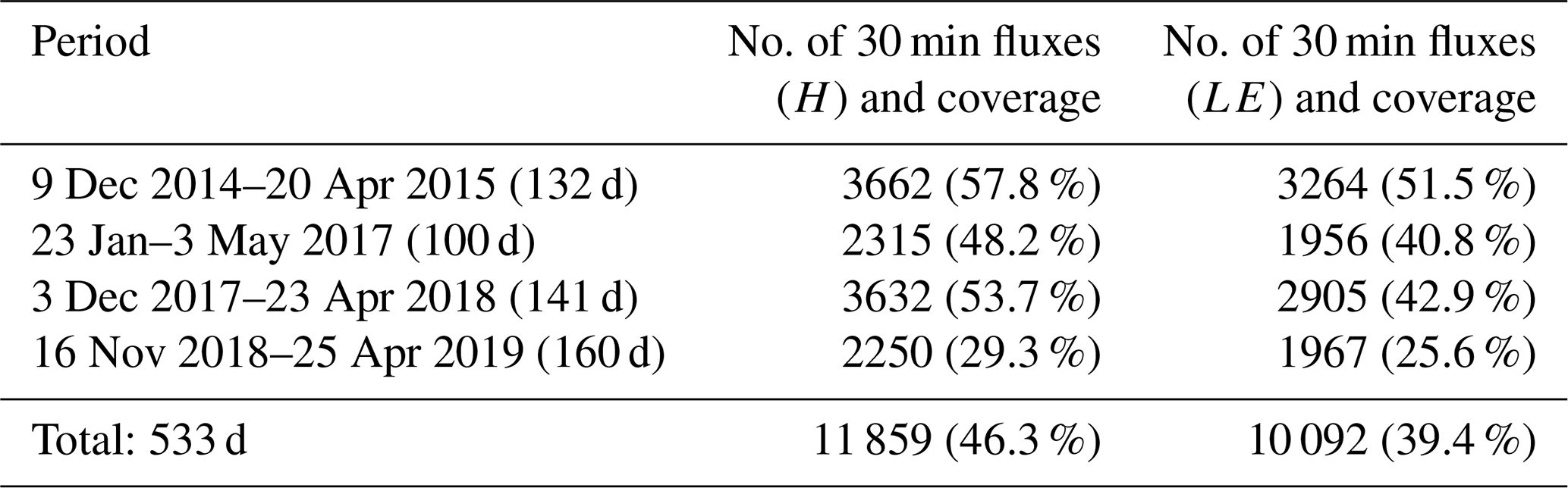
A 2-D footprint analysis was conducted on the data set using the model described in Kljun et al. (2015). Winter 2016–2017 was chosen to be a representative year, and the footprint was calculated from all accepted 30 min flux values from this ice-on season. In Fig. 2 the footprint is presented for three stability classes: stable ($z{L}^{-\mathrm{1}}>\mathrm{0.1}$), neutral ($-\mathrm{0.1}\le z{L}^{-\mathrm{1}}\le \mathrm{0.1}$) and unstable ($z{L}^{-\mathrm{1}}<-\mathrm{0.1}$), where z is the measurement height and L the Obukhov length.

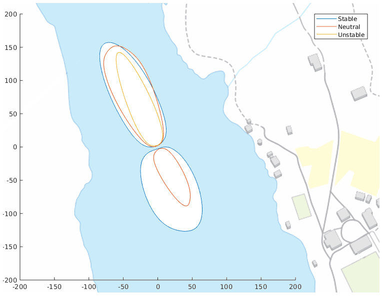
Figure 2 Footprint of EC measurements calculated from the ice-on season 2016–2017 in three stability classes: stable ($z{L}^{-\mathrm{1}}>\mathrm{0.1}$), neutral ($-\mathrm{0.1}\le z{L}^{-\mathrm{1}}\le \mathrm{0.1}$) and unstable ($z{L}^{-\mathrm{1}}<-\mathrm{0.1}$). The plotted lines represent a 80 % footprint. Scale is in meters. Calculated by the footprint script described in Kljun et al. (2015). Map: National Land Survey of Finland, 1 April 2022.

The contour lines represent the limit of the 80 % footprint area. From Fig. 2 it can be seen that the footprint stays well within the boundaries of the lake due to the strongly channeled wind. The 80 % footprint reaches approximately 300 m from the raft in the north–south direction and 100 m in the east–west direction.

2.5 Bulk transfer models

Various forms of the bulk transfer models have been used to estimate vertical turbulent fluxes for decades. In its simplest form the sensible (latent) heat flux is written as a linear function of wind speed, temperature (humidity) difference between the surface and the air and their corresponding transfer coefficients. In order for the bulk fluxes to have the same sign as the EC data have, in this study they are calculated as

$$\begin{array}{}\text{(3)}& {\displaystyle }{H}_{\mathrm{b}}={\mathit{\rho }}_{\mathrm{a}}{c}_p{C}_H(T_{\mathrm{0}}-T_{\mathrm{a}})U,\text{(4)}& {\displaystyle }L{E}_{\mathrm{b}}={\mathit{\rho }}_{\mathrm{a}}{L}_e{C}_E(q_{\mathrm{0}}-q_{\mathrm{a}})U,\end{array}$$

where C_H and C_E are the transfer coefficients of sensible and latent heat, respectively, U is the wind speed, T_a and T₀ are the air and surface temperature, respectively, and q_a and q₀ are the air and surface humidity. In Eq. (4) surface humidity can be assumed to be at saturation due to the watery/icy surface (Leppäranta, 2014).

In this study three different bulk transfer models are compared against EC measurements: one model where the transfer coefficient is kept constant, one developed specifically for open water lake environments (Lake Heat Flux Analyzer) and one developed for sea ice (SHEBA Bulk Turbulent Flux Algorithm for Sea Ice v. 2.0).

2.5.1 Constant transfer coefficient model

The use of a constant transfer coefficient neutral value is a simplified approach, which assumes a negligible effect of atmospheric stability. A range of values between $\mathrm{1.0}\times {\mathrm{10}}^{-\mathrm{3}}$ and $\mathrm{1.5}\times {\mathrm{10}}^{-\mathrm{3}}$ have been reported for C_E and C_H over the years for neutral conditions at 10 m height, for example, in Kagan (1995). Due to the fact that underestimation of turbulent heat fluxes is typical, a value of $\mathrm{1.5}\times {\mathrm{10}}^{-\mathrm{3}}$ was chosen, which corresponds to the high end of the values represented in the literature. This value was then scaled from 10 m height to a height of 1.8 m, resulting in the value of $C_E=C_H=\mathrm{1.8}\times {\mathrm{10}}^{-\mathrm{3}}$ being chosen for our study. Fluxes are then calculated by using Eqs. (3) and (4).

2.5.2 Lake Heat Flux Analyzer (LHFA)

The second model used in this study is the Lake Heat Flux Analyzer software described in Woolway et al. (2015). It was originally developed in order to create a standardized way to compute turbulent flux values acquired from lake measurement networks. The software uses an iterative approach to calculate H and LE with stability corrections based on the MOST, as described in Zeng et al. (1998). As an input to calculate the turbulent fluxes, the model uses air temperature, air humidity, surface temperature and wind speed. The model is developed especially for the open water season, but for the sake of comparison it was decided to include this model as well. The open water optimization is apparent in the calculation of roughness length, which is done according to Smith (1988) and thus includes the Charnock term as well, which in certain conditions takes into account the effect of surface waves. Roughness lengths for heat and moisture are calculated according to Brutsaert (2013).

2.5.3 SHEBA Bulk Turbulent Flux Algorithm for Sea Ice v. 2.0 (SEA‐ICE)

The third model applied in this study was developed for sea ice and is based on the data set acquired from the SHEBA (Surface Heat Budget of the Arctic Ocean) experiment in the Beaufort Sea (Grachev et al., 2007). It is similar to the LHFA model in the sense that it also uses an iterative approach to the stability corrections, but in this model in very stable cases (ζ>1) the flux gradient relations rely on empirical approximations from Grachev et al. (2007), for near-neutral cases no stability correction is applied and for unstable cases the formulation from Paulson (1970) is applied. The roughness length calculation (described in Andreas et al., 2010) is optimized for ice cover, unlike the LHFA, which is optimized for open water. In this study the SEA-ICE model was run at the “winter” setting, corresponding to 100 % ice coverage.

3 Results

3.1 Environmental drivers of diurnal, seasonal and interannual variation of turbulent heat fluxes

Diurnal and seasonal variation as well as the response of the turbulent fluxes to external forcing were studied by dividing the fluxes and meteorological data for all years by month and by hour of day (Fig. 3). Early in the winter (December to February), no diurnal pattern of turbulent fluxes is visible, but as the Sun gets higher over the horizon in the spring and shortwave radiation begins to dominate the surface energy balance, the absolute flux values rise up as well and a diurnal pattern for H (Fig. 3a), LE (Fig. 3b) and wind speed (Fig. 3h) develops. Thus, the ice-on season can be divided into two phases: early winter with no diurnal pattern and late winter with a diurnal pattern with the sunlight affecting the fluxes.

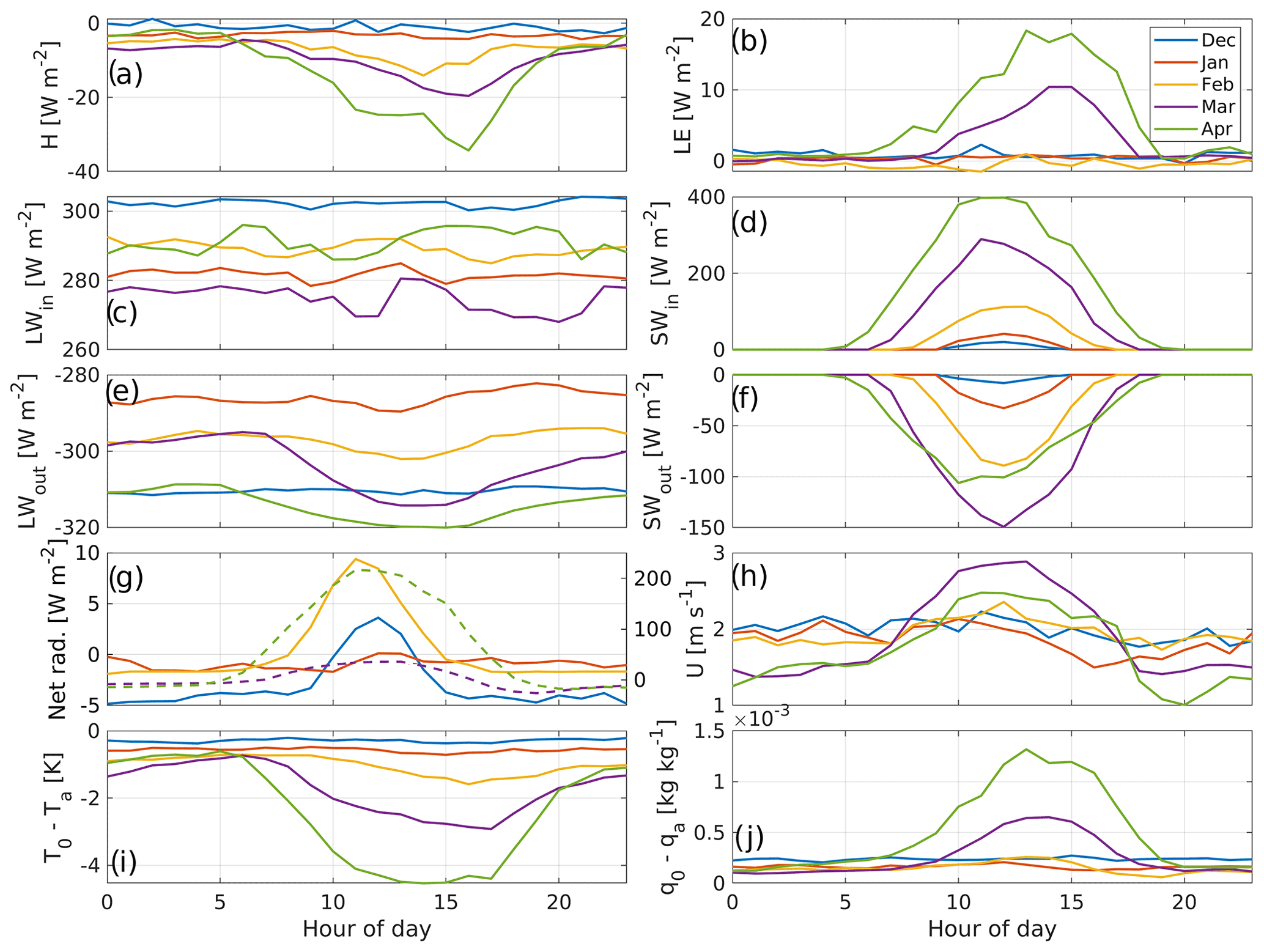
Figure 3 Hourly medians of key variables measured over the lake ice: (a) H and (b) LE measured by EC, all four components of the radiation balance separately (c–f), (g) net radiation, (h) wind speed, (i) temperature difference (T₀−T_a) and (j) specific humidity difference (q₀−q_a). Each curve represents a month of data separated into each hour of the day. Note that the turbulent fluxes have the micrometeorological notation, where negative is flux towards the surface, while net radiation and radiation flux components have the opposite notation. The net radiation plot has two vertical axes to accommodate the higher fluxes of March and April (dashed lines, scale on the right-hand side), and solid lines represent the months from December to February (scale on the left). All times are in UTC+2.

The highest median value of sensible heat flux (−34.3 W m⁻²) is seen in April at 16:00 UTC+2 (Fig. 3a). The flux peak is observed at the same time as the peak of the temperature gradient (Fig. 3i) and lags the maximum of net radiation by about 4 h (Fig. 3g). In the darkest winter months the surface temperature of the ice cover follows the air temperature very closely, thus keeping the sensible heat flux low as well (0 W m${}^{-\mathrm{2}}>H>-\mathrm{5}$ W m⁻²). More difference between the two can occur, especially in the spring, when the air temperature can reach values well above freezing, but the melting ice and snow surface remains close to 0 ^∘C, resulting in negative flux values, i.e., heat transferred from the air into the melting ice surface. Winters at Lake Kuivajärvi (and in southern Finland in general) are defined by cold spells separated by days where the air temperature reaches values above freezing. Peaks in sensible heat flux occur then as well, and the number of such peaks varies from year to year.

A similar pattern is observable for the latent heat flux (Fig. 3b) but with a positive flux developing along with the intensifying radiation instead of a negative flux. During the darkest winter months there is weak median deposition or sublimation of ice or snow at all hours of the day with no clear diurnal pattern (median −1.5 W m${}^{-\mathrm{2}}<LE>\mathrm{1.5}$ W m⁻², or $\sim \pm \mathrm{0.05}$ mm d⁻¹), which turns into daytime evaporation/sublimation in March, when daytime net radiation turns positive. This amount of evaporation or sublimation plays no significant role in the ice and snow mass balance of Lake Kuivajärvi, as the ice cover is on the order of 40 cm with centimeters of snow on top of that, and just the transport of snow by wind can be larger than this evaporation/sublimation. The peak median value, 18.4 W m⁻², is in the afternoon at 14:00 UTC+2, following the peak in the humidity difference (Fig. 3j), again lagging some 4 h behind the peak in net radiation. The diurnal pattern in the humidity difference develops later than that of the temperature difference, and hence the diurnal pattern of LE is visible a month later than that of H.

All time series used in this study are presented in Fig. 4. Interannual differences in the pattern of turbulent heat fluxes occur mostly in the number of cold and warm periods and differences in their lengths. Low temperatures result in low values of LE for two reasons: one is the very dry nature of cold air and the exponential relation of dew/frost point to air temperature and the low vertical gradient of specific humidity which follows from this. The second reason is the low wind speeds that are typically associated with the anticyclonal weather patterns that result in low air temperatures during winters. Low air temperatures result in lower values of H as well, but to a smaller degree than for LE. During winters the stability of the atmospheric boundary layer is mostly stable ($z{L}^{-\mathrm{1}}>\mathrm{0}$), as can be seen in Fig. 4e. In this data set stable conditions were measured for 73 % of the time and unstable conditions for 27 %. The change into the higher late-winter flux values (H and LE >10 W m⁻²) quite consistently begins in mid to late March regardless of year. Peaks of ± 50 W m⁻² are observed almost daily in spring, while in the early winter they are more intermittent and associated with situations where the air temperature reaches values significantly above freezing.

Surface energy balance (Fig. 4f) was calculated as the sum of the four components of radiation and turbulent heat fluxes. Between the months of January and February the surface energy balance had values typically ranging from −50 to 50 W m⁻². After March up until ice-off, surface energy balance varied between −100 and 700 W m⁻². The excess heat in spring is used up in melting of the ice cover as well as heating the underlying water.

The onset of ice cover varies from year to year (range of 45 d in the 4 years studied here), and it is controlled by the meteorological conditions suitable for ice formation. Ice-off is more predictable (range of 13 d), as it is driven by the incoming solar radiation which, regardless of meteorological factors, always begins to dominate the surface energy balance in March.

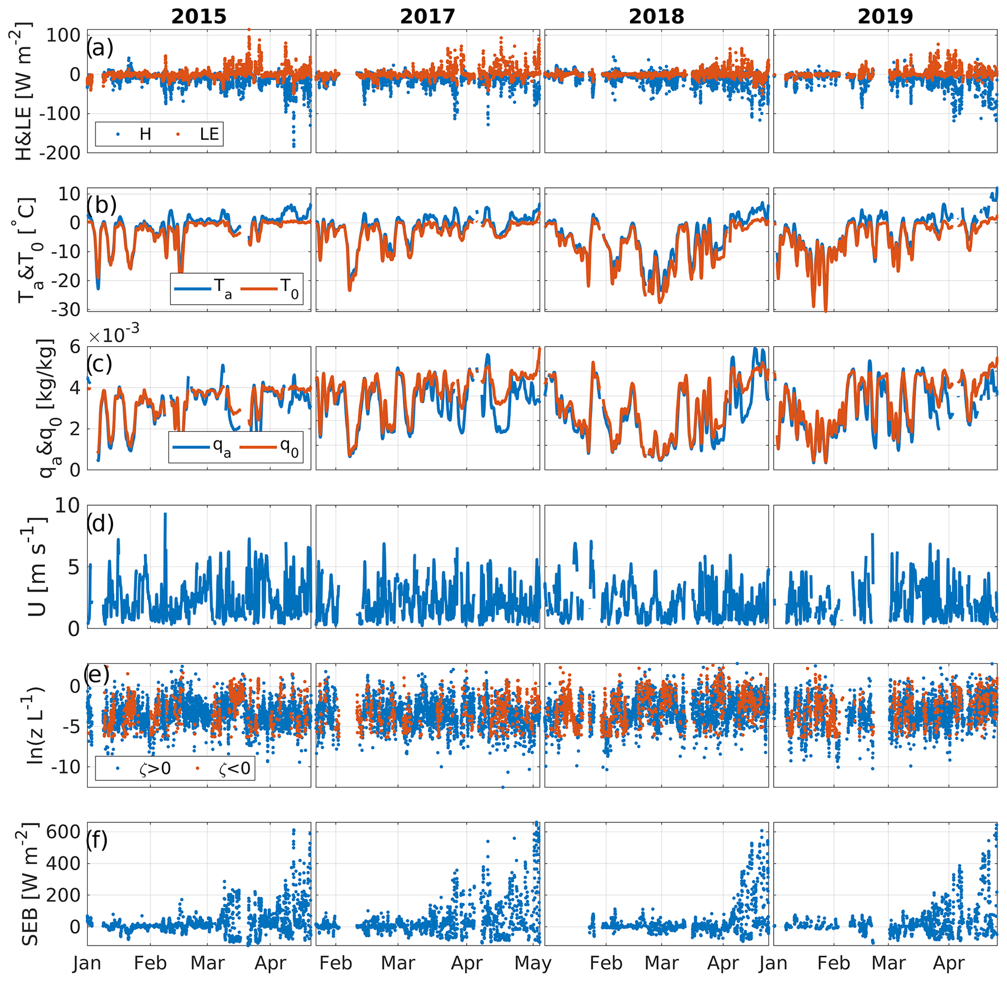
Figure 4 All four winters of (a) turbulent flux data, (b) air and surface temperature, (c) air and surface humidity, (d) wind speed, (e) natural logarithm of stability and (f) surface energy balance (SEB). Each column represents one winter. All data are presented as half-hourly values, except for wind, which is presented as a 6 h moving mean. Note that the surface energy balance notation is such that positive values indicate heat flux into the surface and vice versa.

3.2 Comparison of turbulent fluxes derived by EC and bulk transfer models

For the comparison of the EC data with the models, the data were divided into two sets: one where the surface temperature was below freezing and one where it was above freezing. The data are compared in four ways: first, by box plots where the data are divided, in addition to surface conditions, into each hour of the day (Fig. 5), second, by scatter plots (Figs. 6 and 8), third, by studying the correlation and centered root mean square error (CRMSE) as functions of wind speed, temperature difference and specific humidity difference (Fig. 10), and by Taylor plots (Taylor, 2001), showcasing the differences of correlation, CRMSE and standard deviation between the models and the EC measurements (Figs. 7 and 9). Finally, the behaviors of neutral transfer coefficients are studied in relation to wind speed, and normalized transfer coefficients are examined against atmospheric stability.

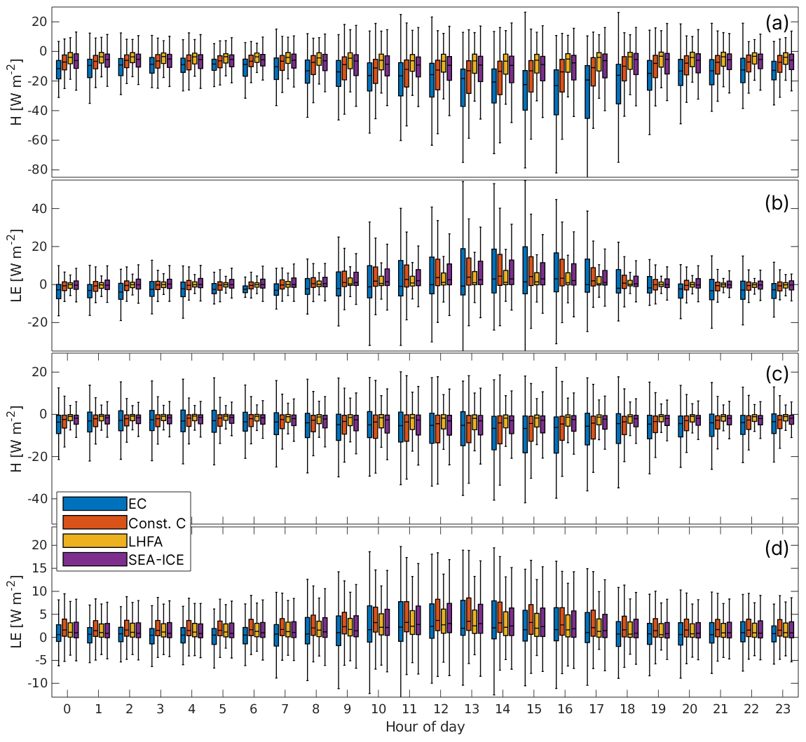
Figure 5 Daily variation of fluxes in EC and the three models. (a) H in melting surface conditions, (b) LE in melting surface conditions, (c) H in freezing surface conditions and (d) LE in freezing surface conditions. The line in the middle of each bar indicates the median, bar edges indicate the 25th and 75th percentiles and the whiskers extending from the bars indicate that 2.7σ or 99.7 % of values are within these boundaries. All times are in UTC+2.

3.2.1  H

Sensible heat flux modeling was observed to function better in melting than freezing surface conditions (Fig. 5a and c). The models also correctly recreate the diurnal cycle of the flux, but underestimation of the flux magnitude as well as standard deviation is common for all of the models studied (Table 2).

The scatter plots (Fig. 6) reveal how all of the models tend to underestimate the EC fluxes of sensible heat by about 15 %–45 % (Table 2). These plots also reveal the tendency of stability-adjusted models to result in near-zero flux, while the EC system measures a significantly non-zero flux. Much higher variability in the model agreement is present in the negative flux values than in positive values, which indicates better agreement during unstable boundary-layer conditions. Of the three models, SEA-ICE performs slightly better than others during unstable conditions (positive flux values for H), as other models show underestimation in comparison to the EC measurements (Fig. 6). Bias in the turbulent flux direction (upward or downward) is more evident during freezing surface conditions (Fig. 6a, c and e) than during melting surface conditions (Fig. 6b, d and f). Taylor plots (Fig. 7) of H reveal that the simpler constant C_H model has higher correlation and smaller CRMSE than either of the stability-adjusted models when compared to the EC measurements. This is true for all surface conditions, but better correlation between models and EC data is found during melting surface conditions.

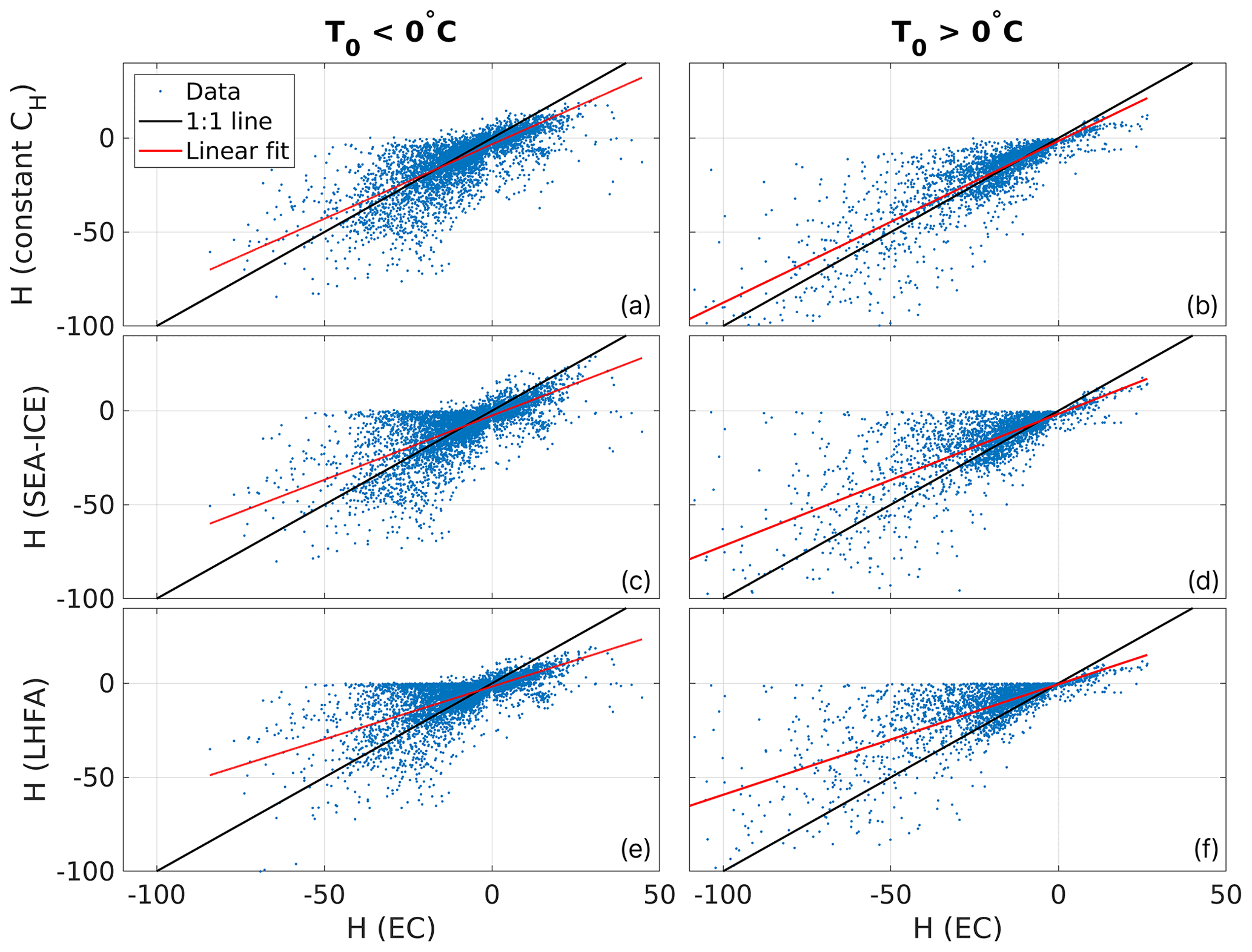
Figure 6 Scatter plots of the 30 min sensible heat flux values of the three included models against corresponding EC measurements. All the axes have a unit of W m⁻². Black line indicates a 1:1 fit and red line the best linear fit. Linear fit parameters are listed in Table 2.

Table 2 Linear fit parameters (ax+b) and statistics of 30 min H values between EC and model data.

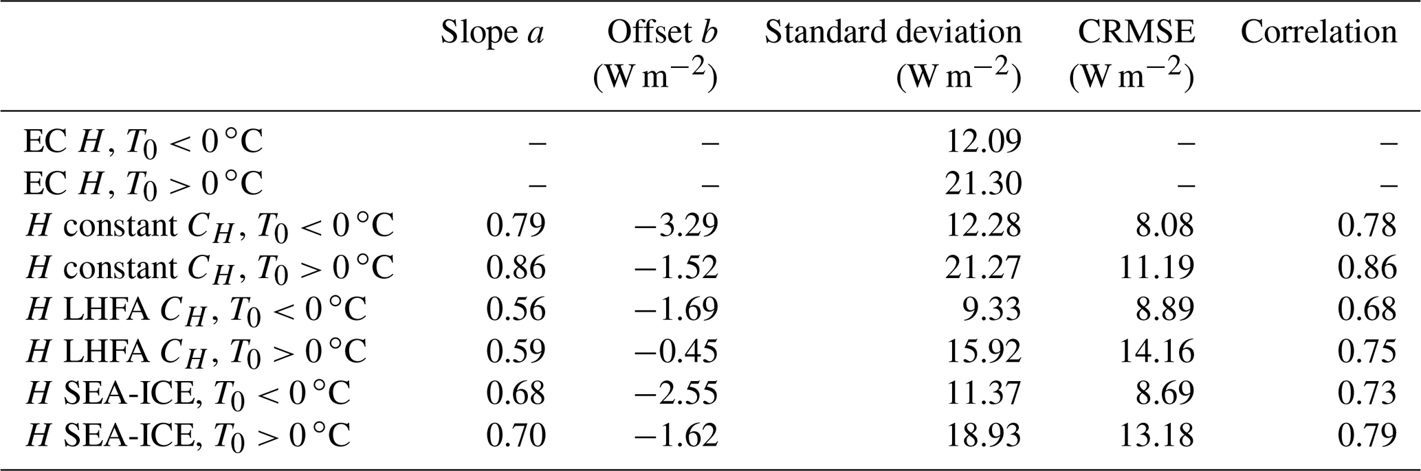
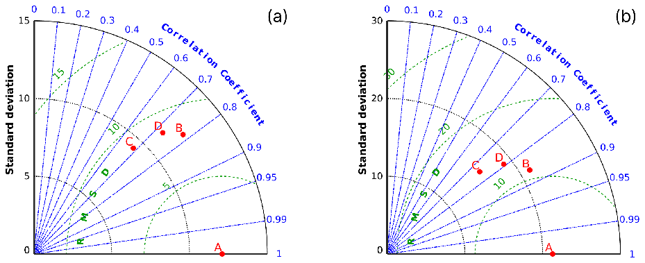
Figure 7 Taylor plots comparing H bulk flux models to EC measurements. Panel (a) has all the cases where the surface was freezing (T₀<0 ^∘C), and in panel (b) are the cases where the surface was melting (T₀>0 ^∘C). A denotes EC measurements, B is the constant C_H model, C denotes the LHFA model and D stands for the SEA-ICE model. Green lines represent isolines of the root mean square error (RMSE), blue lines represent isolines of correlation and dashed black lines are the isolines of standard deviation.

3.2.2  LE

All three models performed the best for LE in freezing surface conditions, with the sign, magnitude and variability all in fairly good agreement with the EC data (Fig. 5b and d) and small variability between the models (Table 3). The LE flux values are also the smallest in these conditions.

The biggest discrepancies between the models and EC data are found during nights in melting surface conditions (Fig. 5b). Here too the largest differences between the models are present. EC data indicate condensation/deposition on the surface for most of the time during nightly melting surface conditions (median of −3 W m⁻² and values of up to −15 W m⁻²). These flux values are almost never reproduced by any of the included models, which typically show a median flux of 1 W m⁻² and peak negative fluxes of −5 W m⁻². The LHFA model performs slightly better than the other two models when LE is negative, but the variability and the magnitude of the fluxes are smaller than the EC measurements. During daytime the range of EC flux values is 2 to 4 times greater than the models, with the greatest standard deviation found in the SEA-ICE model and the lowest found in the LHFA. The LHFA model has consistently a lower median and a smaller standard deviation than the other two models in freezing surface conditions (Fig. 5b and d). The constant C_E model and the SEA-ICE model have very similar performance.

Scatter plots (Fig. 8) reveal that similar patterns of very low bulk fluxes are given when the EC system reports significantly non-zero fluxes. Also, the flux sign is not correctly reproduced sometimes, regardless of surface temperature. The SEA-ICE model results in the best linear fit (Table 3), with the static model performing almost as well and the LHFA resulting in the most underestimation.

Taylor plots (Fig. 9) of LE show that the three models perform quite similarly in regards to correlation and root mean square error, with the greatest differences visible in the standard deviation of the fluxes. By these numbers not one model is clearly better than the others, and they all share the same property of losing some of their predictive ability when the surface is melting. The constant C_E model (Fig. 7b) has a slight advantage in all statistics presented in the Taylor plot over the other two models.

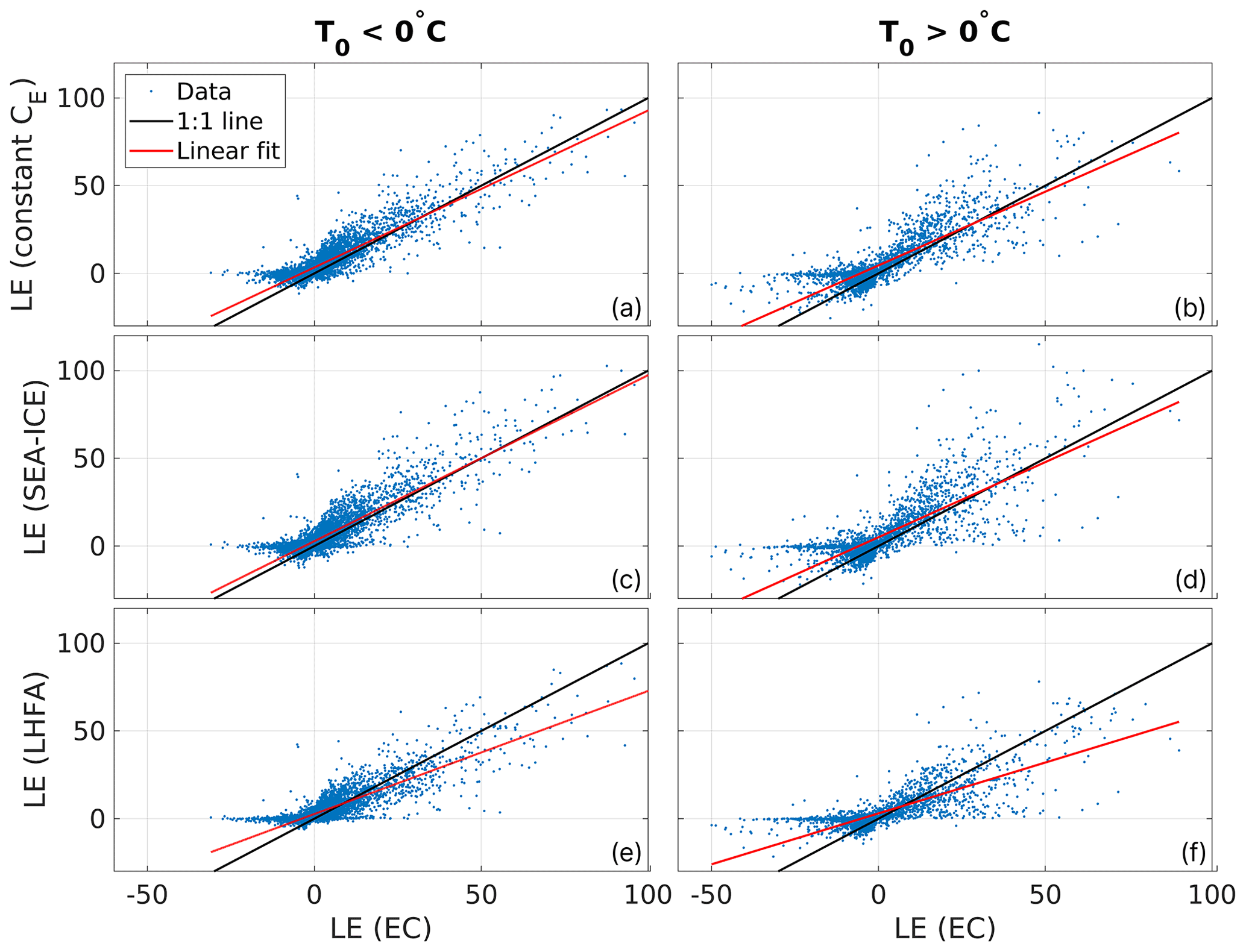
Figure 8 Scatter plots of the three included models against latent heat flux EC measurements. Black line indicates a 1:1 fit and red line the best linear fit. All the axes have a unit of W m⁻². Linear fit parameters are listed in Table 3.

Table 3 Linear fit parameters (ax+b) and statistics of 30 min LE values between EC and model data.

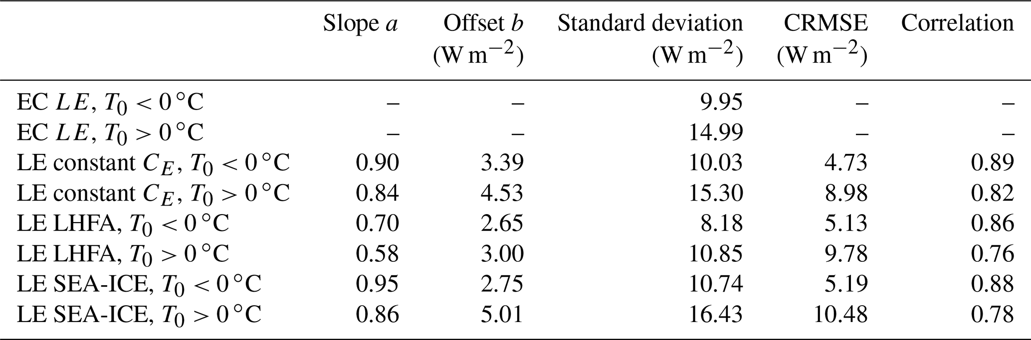
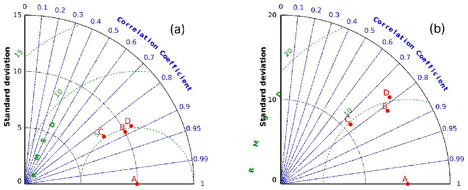
Figure 9 Taylor plots comparing LE flux models to EC measurements. Panel (a) has all the cases where the surface was freezing (T₀<0 ^∘C), and in panel (b) are the cases where the surface was melting (T₀>0 ^∘C). A denotes EC measurements, B is the constant C_E model, C denotes the LHFA model and D stands for the SEA-ICE model.

3.3 Correlation analysis

The behavior of the turbulent heat fluxes was also studied by calculating their correlation and CRMSE as a function of the corresponding meteorological variables. This analysis revealed two conditions where the models have difficulties: low correlation when the temperature–humidity difference between the air and the surface is small and low correlation and high CRMSE during low wind speed. Figure 10a–c show the correlation and error for sensible heat flux as a function of temperature difference between surface and air (T₀−T_a). A clear depression in correlation can be observed at ±0.5 K temperature difference for all the models. The error for all the models is at its lowest then (CRMSE <5 W m⁻²), as sensible heat flux values themselves are small then as well.

Figure 10d–f show the correlation and CRMSE of latent heat flux against the difference of specific humidity between surface and air. Similarly to the temperature difference, low correlation is observed below $\mathrm{0.2}\times {\mathrm{10}}^{-\mathrm{3}}$ kg kg⁻¹ humidity difference. It can be seen that the correlation remains at around 0 for negative humidity differences as well, i.e., in cases where deposition of water/ice should occur over the lake ice surface. This behavior was noted previously in Fig. 8 as the inability of the models to reproduce the scale of nighttime negative EC flux values of LE.

The second type of cases with both high error and low correlation can be found for low wind speed cases (U≤2 m s⁻¹) shown in Fig. 10g and h. Bulk models always result in low fluxes in these cases, which follows from the linear dependency of the bulk flux on the wind speed (Eqs. 3 and 4), but EC measures sometimes relatively high fluxes of around ±20 W m⁻² in these conditions. The expected result would have been a similar situation to that with the temperature and humidity: in low wind conditions correlation drops as the absolute value of the flux drops near 0. In these previously described cases, CRMSE would also remain small. Figure 10h shows that, while correlation drops significantly in low wind conditions, CRMSE increases when compared to cases between 2 and 6 m s⁻¹ (Fig. 10g). This behavior is present in all stability conditions.

Figure 10 The centered root mean square error (CRMSE) (a, d, g) and correlation (b, e, h) of H (solid line) and LE (dashed line) for 100 equidistant bins of temperature difference, humidity difference and wind speed for each of the three models (blue for constant $C_{H/E}$, red for LHFA and black for SEA-ICE). The lowest row of figures (c, f, i) shows histograms of temperature and humidity difference and wind speed values.

3.4 Transfer coefficients

The behavior of the transfer coefficients for heat (C_H) and humidity (C_E), estimated from observations and models, was studied in two ways: first by plotting the neutral values ($-\mathrm{0.1}<z{L}^{-\mathrm{1}}<\mathrm{0.1}$) of transfer coefficients as a function of wind speed (Fig. 11) and then by investigating how the normalized transfer coefficients depend on atmospheric stability (Fig. 12).

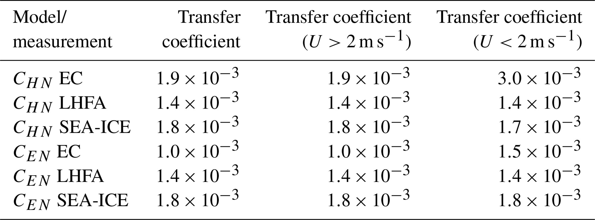
Neutral values of transfer coefficients, estimated from observations (EC), were characterized by similar patterns in their wind speed dependence (Fig. 11). At high wind speeds (U>2 m s⁻¹), C_HN and C_EN remained at relatively constant values of $\mathrm{1.9}\times {\mathrm{10}}^{-\mathrm{3}}$ and $\mathrm{1.3}\times {\mathrm{10}}^{-\mathrm{3}}$, respectively, which are in relatively good agreement with model values. Both transfer coefficients increased towards the lowest wind speeds. The strongest increase was found for C_HN, which was more than twice as high ($\mathrm{4.8}\times {\mathrm{10}}^{-\mathrm{3}}$) at the lowest wind speed bin. A similar but less pronounced increase was observed for C_EN, whose value at the lowest wind speed bin was $\mathrm{2.9}\times {\mathrm{10}}^{-\mathrm{3}}$. Both of the dynamic models (LHFA and SEA-ICE) fail to reproduce this increase during low wind speed, showing nearly constant values for low and high wind speed ranges (Table 4).

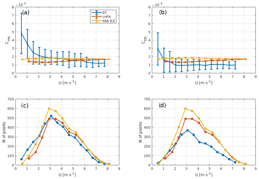
Figure 11 Dependency of neutral transfer coefficients ($-\mathrm{0.1}<z{L}^{-\mathrm{1}}<\mathrm{0.1}$) as a function of wind speed. Panels (a) and (b) show this dependency for heat (C_HN) and evaporation (C_EN), as estimated from models (LHFA and SEA-ICE) and EC observations (EC), respectively. The error bars indicate the standard deviation in the bins. Panels (c) and (d) show the distribution of neutral conditions as a function of wind speed. C_HN data were filtered for small temperature differences ($|T_{\mathrm{0}}-T_{\mathrm{a}}|<\mathrm{0.5}$ K), and C_EN data were filtered for very small and negative values of the humidity difference ($q_{\mathrm{0}}-q_{\mathrm{a}}<\mathrm{2}\times {\mathrm{10}}^{-\mathrm{4}}$ kg kg⁻¹). The 30 min values of coefficients were also not included in case of very low wind speed (U<0.5 m s⁻¹). Bins with fewer than 10 values were not included. The values are for the measurement height of 1.8 m.

Table 4 Neutral ($-\mathrm{0.1}\le z{L}^{-\mathrm{1}}\le \mathrm{0.1}$) transfer coefficients estimated at z=1.8 m.

The dependency of transfer coefficients, normalized by their neutral values ($-\mathrm{0.1}\le z{L}^{-\mathrm{1}}\le \mathrm{0.1}$), on stability parameter zL⁻¹ is presented in Fig. 12. Transfer coefficients for H, calculated from measurements, show slightly higher values than the model ones, and they do not follow the expected dependency on stability, as $C_H/C_{HN}$ estimated from EC measurements does not follow the expected decreasing trend for $z{L}^{-\mathrm{1}}>\mathrm{0}$. During unstable conditions $C_H/C_{HN}$ values acquired by EC show an increasing trend but on average have higher values than the bulk models. C_E determined from measurements shows good agreement during unstable conditions and increasingly higher values than the models towards higher stability.

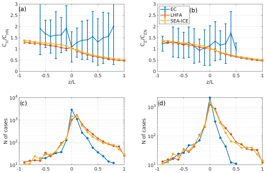
Figure 12 Normalized and binned values of transfer coefficients as a function of the stability parameter for C_H (a) and C_E (b). C_H data were filtered for small temperature differences ($|T_{\mathrm{0}}-T_{\mathrm{a}}|<\mathrm{0.5}$ K) and C_E data were filtered for very small and negative values of the humidity difference ($q_{\mathrm{0}}-q_{\mathrm{a}}<\mathrm{2}\times {\mathrm{10}}^{-\mathrm{4}}$ kg kg⁻¹). The 30 min values of coefficients were also not included in case of very low wind speed (U<0.5 m s⁻¹). Bins were rejected if they had fewer than 10 values within them. Panels (c) and (d) correspondingly present the distribution of transfer coefficient values as a function of the stability parameter.

4 Discussions and conclusions

Turbulent heat fluxes were studied with an EC setup for four winters over the ice cover of a boreal lake, and these results were compared to three bulk aerodynamic models, one that does not take into account the atmospheric stability and two that do take it into account. Our data set spanning four ice-on seasons provided a good opportunity to verify and compare the accuracy of bulk transfer models over direct measurements of turbulent heat fluxes by an EC setup on seasonal lake ice cover.

The best agreement between measured and modeled fluxes of H and LE was found for cases with high wind speed and large water–air temperature and humidity differences. Lake ice surface is a challenging environment for eddy covariance due to the relatively low amount of turbulence in the air above it. This is for several reasons: the boundary layer is stable for most of the time during winter, which leads to underdeveloped turbulence and decoupling of the flow from the surface, the surface has a very low roughness and fluxes are usually low. Despite these challenges, the EC setup was able to record good-quality flux values in a wide range of meteorological states, and the data coverage was sufficient.

The bulk aerodynamic method is technically and computationally much simpler than the eddy covariance method, but it comes with some limitations. The greatest error-producing effect can be attributed to the fact that estimating the skin temperature of a snowy surface is difficult, which has been previously reported as a major issue in modeling turbulent heat fluxes over snow and ice (Franz et al., 2018; Bourassa et al., 2013). This is due to melting and refreezing and the consequent horizontally heterogeneous changes in the surface properties, like albedo, emissivity and phase (liquid or frozen). Errors in determination of the surface temperature affect both sensible and latent heat flux computation, especially when the difference between air and surface is small. It results in incorrect surface humidity values, which is an exponential function of the surface temperature and thus very sensitive to errors. Also, the emissivity ϵ of the ice/snow surface is difficult to determine accurately, and it can change with the metamorphosis of snow (Hori et al., 2006), which happens constantly over the course of the winter. Thus, the calibration and proper installation of especially the longwave radiation sensors is very important in campaigns performed over ice or snow. Due to the horizontally and vertically heterogeneous nature of the surface, point measurements performed in one location, like net radiation, are not always representative of the whole lake, and there is a possibility that very biased results for the surface albedo and outgoing longwave radiation are recorded, especially during the melting period. This partially explains differences in EC and bulk flux results, as the footprint of EC measurements is at least an order of magnitude larger than the source area measured by the radiation sensors.

Similar behavior of the models studied here has been observed in previous studies. In Franz et al. (2018) it was noted that the LHFA and SEA-ICE models tended to underestimate and result in lower standard deviation than the turbulent heat fluxes acquired by EC over a Siberian thermokarst lake, which is in line with the results of our study. Correlation of these models ranged between 0.7 and 0.9 over the thermokarst lake, which is similar to our findings.

In a study conducted over landfast sea ice (Raddatz et al., 2015), the bulk transfer models were seen to underestimate negative fluxes, but unlike our results, they were found to overestimate positive fluxes for both H and LE. Correlation coefficients were found to be slightly larger (0.88) for LE than for H (0.82), which is similar to our results. The same study reported better accuracy of models with a constant transfer coefficient over dynamic coefficients in the winter–spring transition period, although in general they observed the dynamic model performing marginally better over the static one. Differentiation between frozen and melting surfaces was not performed in the aforementioned studies, but the results of our study indicate that modeling of H works better in melting conditions, while the opposite holds for LE.

Issues with the bulk algorithms were noticed as low correlation and high error in low wind speed conditions, which can possibly be explained by non-local effects on turbulence above the lake. In Barskov et al. (2019) it was shown that a sharp decrease in aerodynamic roughness, like the transition between dense forest and lake ice commonly found on boreal lakes, can cause significant fluxes on EC measurements, while bulk algorithms show very low values. When the wind blows from the forest towards the lake, a significant increase in turbulent kinetic energy is observed near the center of the lake, and heat and moisture are transported from the upper boundary layer towards the surface. Bulk algorithms do not take this local violation of MOST into account and thus fail to reproduce these situations.

Discrepancies at low wind speed can also be seen when studying the neutral transfer coefficients as a function of wind speed. Dependency of neutral transfer coefficient values on wind speed have been studied previously during the open water season, most recently and applicably on Lake Kasumigaura in Japan (Wei et al., 2016). In this study, observations similar to ours were made, namely, that the transfer coefficients increase during low wind speed conditions (U<3 m s⁻¹). This effect has been attributed to several possible mechanisms, but the study performed over Lake Kasumigaura showed that capillary waves and the averaging method used for the calculation of mean wind speed only had a small effect on the increase in neutral transfer coefficients towards lower wind speed. Larger effects were noted to be most likely caused by increases in turbulent kinetic energy over the lake in low wind speed conditions. Our data are in agreement, as in our case the coefficients increase in the same range of wind speed, and any effect of waves and underlying currents in the water can be excluded as possible reasons due to the ice cover.

Neutral values in high wind speeds were all within the same range between the bulk models and EC. In high wind speed conditions (U>2 m s⁻¹), the neutral transfer coefficient for heat and water vapor calculated from EC observations is very close to the values estimated from the models, with slightly lower values for evaporation than for heat, which indicates dissimilarity between temperature and humidity.

The fact that EC observations were only made on one level also somewhat limited our ability to perform analysis regarding, for example, the roughness length over the lake ice cover or the applicability of the logarithmic profile for wind speed and scalars. With multiple levels of measurement, cases where MOST is locally violated could be identified much better.

Although the stability-corrected bulk transfer models have a sounder physical and theoretical basis than an uncorrected static model has, it is possible to get lower agreement between EC and dynamic models than between EC and static models. This is not to say that the stability-corrected models are inherently wrong but that conditions violating MOST are not uncommon over lakes. Thus, although generally good, turbulent heat flux values obtained by bulk transfer models on very small lakes surrounded by forest generally underestimate the flux as the heterogeneity of the surrounding environment and measurement errors over the complex and dynamic ice cover causes incorrect output of the models in certain conditions.