the Creative Commons Attribution 4.0 License.
the Creative Commons Attribution 4.0 License.
 | 20 Jun 2022
A map of global peatland extent created using machine learning (Peat-ML)
Koreen Millard
Matthew Fortier
R. Scott Winton
Javier M. Martín-López
Hinsby Cadillo-Quiroz
Darren Kidd
Louis V. Verchot
Peatlands store large amounts of soil carbon and freshwater, constituting an important component of the global carbon and hydrologic cycles. Accurate information on the global extent and distribution of peatlands is presently lacking but is needed by Earth system models (ESMs) to simulate the effects of climate change on the global carbon and hydrologic balance. Here, we present Peat-ML, a spatially continuous global map of peatland fractional coverage generated using machine learning (ML) techniques suitable for use as a prescribed geophysical field in an ESM. Inputs to our statistical model follow drivers of peatland formation and include spatially distributed climate, geomorphological and soil data, and remotely sensed vegetation indices. Available maps of peatland fractional coverage for 14 relatively extensive regions were used along with mapped ecoregions of non-peatland areas to train the statistical model. In addition to qualitative comparisons to other maps in the literature, we estimated model error in two ways. The first estimate used the training data in a blocked leave-one-out cross-validation strategy designed to minimize the influence of spatial autocorrelation. That approach yielded an average r2 of 0.73 with a root-mean-square error and mean bias error of 9.11 % and −0.36 %, respectively. Our second error estimate was generated by comparing Peat-ML against a high-quality, extensively ground-truthed map generated by Ducks Unlimited Canada for the Canadian Boreal Plains region. This comparison suggests our map to be of comparable quality to mapping products generated through more traditional approaches, at least for boreal peatlands.
- Article
(25554 KB) - Full-text XML
- BibTeX
- EndNote


The works published in this journal are distributed under the Creative Commons Attribution 4.0 License. This license does not affect the Crown copyright work, which is re-usable under the Open Government Licence (OGL). The Creative Commons Attribution 4.0 License and the OGL are interoperable and do not conflict with, reduce or limit each other.
© Crown copyright 2022
Peatlands are estimated to cover about three percent of the land surface but contain approximately a third of the soil carbon and roughly a tenth of surface freshwater (Joosten and Clarke, 2002; Jackson et al., 2017) and are vulnerable to destabilization due to climate change and anthropogenic pressures, including drainage and land use change. Their importance in the carbon and hydrologic cycles motivates their inclusion in Earth system models (ESMs) to better understand their potential impact on the climate system. Since the land surface of ESMs is grid based, a prerequisite for integrating peatlands into these models is to define the location and the fractional cover of peatlands on the model grid. However, peatlands have generally been overlooked in landscape databases and their mapping remains challenging (e.g. Krankina et al., 2008; Minasny et al., 2019).
As peatlands are commonly considered a type of wetland that contains large amounts of organic carbon in the soil, several studies have set peatland distribution based on maps of soil organic matter density (e.g. Wania et al., 2009; Bechtold et al., 2019; Hugelius et al., 2020). However, using soil organic matter databases alone in determining peatland distribution tends to overlook the vegetation and subsurface hydrology, but most importantly they rely heavily on the fidelity of the soil carbon dataset. Another approach has been to use a soil map together with global wetland maps or inundation extent maps (e.g. Köchy et al., 2015). These wetland and inundated area databases have mostly been produced through mapping of shallow surface water based on remote-sensing data, as in the Global Inundation Extent from Multi-Satellites initiative (GIEMS; Prigent et al., 2007; Papa et al., 2010) and the Surface WAter Microwave Product Series (SWAMPS; Schroeder et al., 2015), or land cover mapping using surface observations and moderate-resolution imaging spectroradiometer (MODIS) data, as in the Global Lake and Wetlands Database (GLWD-3; Lehner and Döll, 2004). These wetland mapping products are, however, of limited utility for peatland modelling applications as they generally do not agree well amongst themselves (Melton et al., 2013), which is also the case for peatland mapping products (as is discussed later) and may exhibit biases depending on how they were generated (see discussion in Bohn et al., 2015). In addition, in the boreal zone and some areas of the tropics such as the Amazon (Lähteenoja and Roucoux, 2010), some peatlands are not inundated, and thus using hydrological characteristics alone can underestimate their extent (Matthews, 1989; Prigent et al., 2007). Other studies, such as Largeron et al. (2018) or Leifeld and Menichetti (2018), have used a global peatland distribution map derived from a paleontological perspective (Yu et al., 2010). However, Yu et al. (2010) is an estimated map of binary polygons that does not provide quantitative information on fractional coverage. The most comprehensive global peatland map we are aware of is PEATMAP (Xu et al., 2018), which was generated through a meta-analysis of regional-scale mapping products of varying spatial resolution and provenance (general land cover maps, soil databases, and a hybrid expert system). This dataset is not well suited as a peatland mask for ESM use as the resolution of some of its parent datasets leaves large polygons of complete peatland cover in regions where this is unlikely and it misses peatlands in regions where peatland coverage is known to exist, e.g. the Republic of Sakha (Yakutia, Russia), as it is dependent upon mapping products existing for each region.
In describing their dataset, Yu et al. (2010) state that, “accurate true peatland coverage and distribution is not available for many mapped regions”. Over a decade after the publication of Yu et al. (2010), this statement remains accurate. Peatlands have traditionally been mapped through field surveys and manual inspection of aerial photography (e.g. Tarnocai et al., 2011). These approaches are costly and labour intensive and become impractical as the study region becomes large or remote. As noted by Loisel et al. (2017), it is also difficult to distinguish upland forests from forested peatlands in the boreal region and between (sub)arctic tundra vegetation and peatlands in the higher latitudes using aerial photography. Digital soil mapping (DSM) is an alternative approach to determining global peatland cover. DSM techniques typically combine field surveys with peatland covariates and statistical models to produce maps of predicted peatland area (McBratney et al., 2003). Following Minasny et al. (2019), the peatland covariates useful to DSM can be determined from the drivers of peatland formation, indicators of peat presence, and sensors able to measure the indicators.
The drivers of peatland formation are scale dependent (Limpens et al., 2008) and thus the intended spatial extent and mapping resolution of the DSM product is an important consideration. For DSM on a regional to global scale, as is the case when mapping for ESM use, the principal drivers of peatland formation are climate, vegetation, and terrain. Minasny et al. (2019) suggest, for these drivers at this spatial scale, that the indicators of peatland presence are climate data (primarily temperature and precipitation); land use and land cover information; and elevation, slope, and terrain attributes. Possible sensors for regional- to global-scale mapping include optical and radar imagery, topographic remote-sensing data (digital elevation models, DEMs), and climate datasets. The statistical models used as part of DSM vary, but here we use a machine learning (ML) algorithm to derive a global map of peatland extent intended for use in ESM applications. As field surveys are impractical to conduct on a global scale, we rely upon peatland mapping studies on regional scales to train our ML models and evaluate their results. In Sect. 2 we define peatlands in the context of our mapping approach and describe the datasets used for model training and the ML approach and algorithms used. Section 3 discusses the results of the ML algorithms and our model performance estimation strategy and limitations of our approach. Section 4 presents our overall conclusions.
2.1 Definition of peatlands
As there is no single, universally adopted definition of peatlands, we follow Joosten and Clarke (2002) in defining them as areas with or without vegetation that contain a naturally accumulating peat layer at the surface. While the definition of peat, as defined by the percent dead organic material by dry mass, varies considerably in the literature (e.g. Gumbricht et al., 2017; Page et al., 2011), we choose a more inclusive lower minimum value of 30 % to ensure we can capture the diversity of global peatlands. When using peatland mapping datasets that contain continuous peat depths (Sect. 2.3), we have used a minimum thickness of 30 cm of peat to delineate peatlands, similar to Gumbricht et al. (2017). This depth limit is the most common amongst national datasets (but see discussion on exceptions or the implications of different values in Loisel et al., 2017).
2.2 Data acquisition and preparation
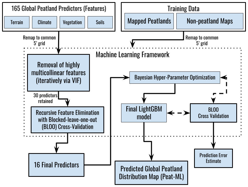
The general process of data preparation, model training, and evaluation is illustrated in Fig. 1. All training (regional peatland and non-peatland mapping products) and predictor (peatland covariates) data were converted from their native format (commonly GeoTiff rasters or vector-based GIS formats such as shapefiles) to netCDF format and remapped onto a common 5 arcmin (ca. 0.0833∘, corresponding to 9.26 km at the Equator and 4.63 km at 60∘ N) grid using climate data operators (CDO; Schulzweida, 2020), a geospatial data abstraction software library (GDAL/OGR; GDAL/OGR contributors, 2021), and/or netCDF Operators (NCO) (Zender, 2008). The original resolutions of the data sources are each listed below. All ML runs and evaluations were performed on the 5 arcmin grid.
2.2.1 Predictors (peatland covariates)
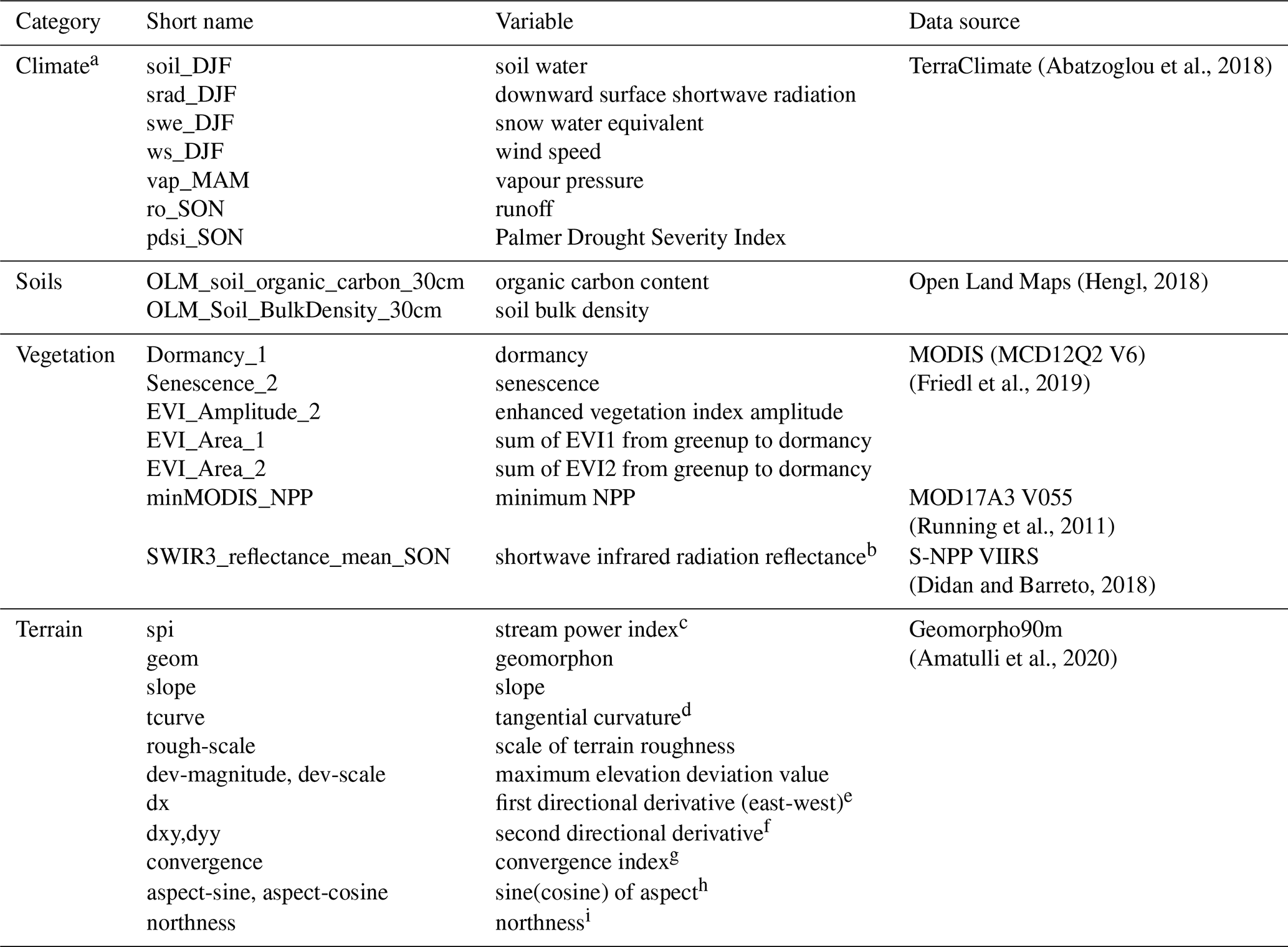
We used a suite of predictors that fell into four main types: climate, soils, vegetation, and terrain (geomorphology). Table 1 lists each predictor grouped by predictor source and type. The climate, vegetation, and soil predictors were extracted from the Google Earth Engine data catalogue (Gorelick et al., 2017). The geomorphological dataset was downloaded directly from its authors' website (Amatulli et al., 2020, last access: 16 January 2020). Sampling across the different years provided by each dataset is assumed to be relatively unimportant as peatland extent is not highly dynamic across decadal timescales, especially considering the scale of our grid cells (Loisel et al., 2013). An additional predictor was the calculated length of the longest day of the year (hours) for each cell on the 5 arcmin grid. The longest day of the year could be used by the model to determine tropical versus extratropical regions.
The climate predictors were derived from the TerraClimate dataset (Abatzoglou et al., 2018). TerraClimate is available at high spatial resolution (∘) and provides monthly climate and climatic water balance variables spanning the 1958 to 2015 period. TerraClimate uses the WorldClim dataset for high spatial resolution climatic normals, which is combined with the time-varying climate of the Climate Research Unit Ts4.0 (CRU Ts4.0; Harris et al., 2020), where the time-varying anomalies of CRU Ts4.0 are interpolated to the high-resolution climatology of WorldClim. The Japanese 55-year reanalysis (JRA55; Kobayashi et al., 2015) is used to fill in where CRU Ts4.0 has no climate stations contributing to its record (such as parts of South America, Africa, and smaller islands) and was the sole data source for solar radiation and wind speeds. Abatzoglou et al. (2018) notes that the water balance model, used to generate some of the variables listed in Table 1, is simple and does not account for vegetation heterogeneity or their physiological response under varying environmental conditions. For the climate predictors, we computed seasonal means across the available years, i.e. December–February (DJF), March–May (MAM), June–August (JJA), and September–November (SON). Given that these seasonal means are likely less important in tropical regions, we did investigate using annual minimum and maximum values in place of seasonal ones but did not see a significant impact on predicted peatland fractional cover.
Soil predictors were obtained from the 250 m resolution OpenLandMap (Hengl, 2018) including soil bulk density (kg m−3), clay content (%), sand content (%), organic carbon content (%), and soil water content at field capacity (33 kPa). These soil variables are derived from an ensemble of machine learning algorithms trained on a global compilation of soil profiles (Hengl and MacMillan, 2019). We used the 30 cm depth estimate for all soil variables.
Terrain information is provided by the 250 m resolution version of Geomorpho90m (Amatulli et al., 2020) for 17 different geomorphometry variables describing numerous aspects of the land surface (see Table 1). This geomorphology dataset has an original resolution of 90 m, the same resolution as the Multi-Error-Removed Improved Terrain (MERIT) DEM (Yamazaki et al., 2017) from which it was derived. MERIT-DEM is a merged and error-corrected product based on the ALOS World 3D – 30 m (AW3D30) and Shuttle Radar Topography Mission (SRTM3) datasets.
Information about the vegetation state was provided by several datasets. Shimada et al. (2014) created a seamless global mosaic image from the Phased Array type L-band Synthetic Aperture Radar (PALSAR/PALSAR2). This image was created with 25 m grid cells on an annual timescale. In creating the mosaic, at each location within a year the images chosen were those showing minimum response to surface moisture. The images were then ortho-rectified, slope corrected, and had a destriping procedure to equalize differences between strips that could occur due to conditions at time of acquisition. As the dataset's intended purpose was to provide a global mask of forest cover (Shimada et al., 2014) soil moisture differences were purposefully minimized, and thus this dataset is likely of more limited use to predict peatland extent than would otherwise be expected for an L-band radar product (Izumi et al., 2019; Touzi et al., 2018). However, likely due to the significant computational effort required to produce a global L-band product, we are not aware of another product publicly available.
The MODIS Terra net primary productivity product (MOD17A3.055 NPP) is available annually on a 1 km grid (Running et al., 2011). This version of MODIS NPP (v. 5.5) is corrected for issues relating to cloud-contaminated MODIS leaf area index fraction of photosynthetically active radiation (LAI-FPAR) inputs to the MOD17 algorithm. We averaged the data over the available 2000–2015 period.
Vegetation indices are provided by the Suomi National Polar-Orbiting Partnership (S-NPP) NASA Visible Infrared Imaging Radiometer Suite (VIIRS) product VNP13A1, which is generated by selecting the best pixel at 500 m resolution over a 16 d acquisition period. The VIIRS data are generated for three vegetation indices including the normalized difference vegetation index (NDVI), which uses both red and near-infrared (NIR) bands, and two enhanced vegetation indices (EVI, EVI2), which also include the blue band with EVI2 designed for intercomparison with other EVI products that do not use a blue band (Table 1). EVI is more sensitive to canopy cover, while NDVI is more sensitive to chlorophyll (Huete et al., 2002). All snow, cloud, or cloud shadow pixels and any pixels that were not excellent, good, or acceptable quality (according to the dataset's quality flags) were excluded. Given the original data do not have composite monthly values, the mean, minimum (min), maximum (max), and standard deviation (SD) were all calculated based upon all values within a year and then the average was taken across all years.
Vegetation phenology information is provided by the MCD12Q2 V6 Land Cover Dynamics product (Friedl et al., 2019). The MODIS vegetation phenology product provides phenological information such as the dates of green-up, peak, and senescence along with variables related to the range and summation of the EVI (see Table 1). Since this is an annual product the mean, min, max, and SD values are calculated across all years.
We also considered the global surface water (GSW) dataset of Pekel et al. (2016) but did not include it as a predictor dataset. We found this dataset to be unsuitable for peatland prediction due to its reliance on Landsat imagery. Treed peatlands, peatlands smaller than 30 m by 30 m, and peatlands where the water table is below the peat surface, such as bogs, would not be well captured by GSW. A visual inspection of GSW over some of our training regions (see Sect. 2.3) showed poor correlation between GSW water presence and mapped peatland area.
(Abatzoglou et al., 2018)(Hengl, 2018)(Amatulli et al., 2020)(Shimada et al., 2014)(Running et al., 2011)(Didan and Barreto, 2018)(Friedl et al., 2019)Table 1Potential peatland co-variates used as predictor variables for the ML algorithms to predict peatland fractional cover. The treatment of variables is discussed in Sect. 2.2.1. The predictor variables in bold were selected for the final model (see Sect. 2.4.3).
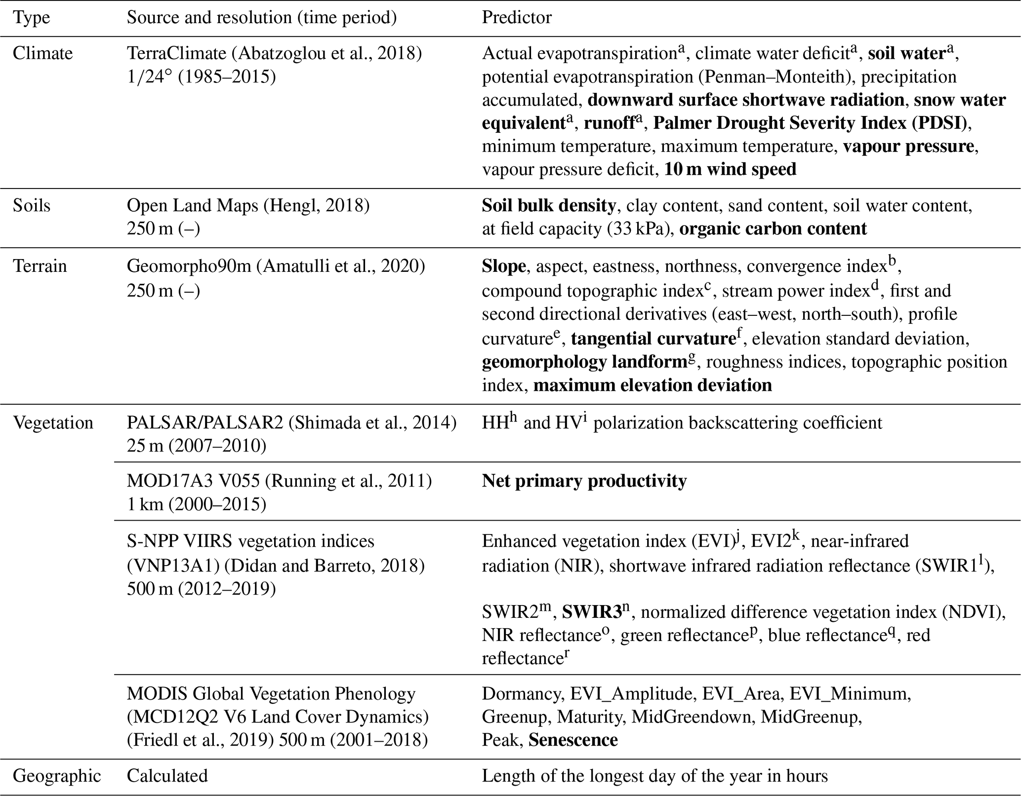
a Derived using a one-dimensional soil water balance model. b Ranges between 100 for sinks (convergent areas) and −100 for ridges (divergent areas). Flat areas are 0. c Also known as topographic wetness index (Beven and Kirkby, 1979). d Defined as the product of the tangent of the local slope angle and the upstream catchment area. e Measures the rate of change of a slope along a flow line. Convex slopes accelerate water flowing along them while concave slopes decelerate flow. f Measures the perpendicular rate of change to the slope gradient. This captures the convergence (concave curvature) and divergence (convex curvature) of flow across a surface. g For example, flat, spur, valley, calculated using morphometry techniques based on pattern recognition. h Horizontal transmit and horizontal receive. i Horizontal transmit and vertical receive. j Three-band enhanced vegetation index. k Two-band EVI using only red and NIR band. l 1230–1250 nm. m 1580–1640 nm. n 2225–2275 nm. o 846–885 nm. p 545–656 nm. q 478–498 nm. r 600–680 nm.
2.3 Training data
For training and testing the machine learning model, peatland fractional cover was selected as the target variable. However, accurate estimates of peatland fractional cover are not widely available, as discussed in Sect. 1. Recently, Minasny et al. (2019) reviewed the present state of peatland mapping. They found 90 recent studies mapping peatlands, with many delineating peatland extents using ecological and environmental field studies in combination with land cover from remote sensing; however, the studies seldom conduct validation of their mapping, and uncertainty estimates are rare (e.g. Table 4 in Minasny et al., 2019). Additionally, the definition of peat can vary between countries and studies (e.g. Table 2 in Minasny et al., 2019), making assembling an internally consistent global dataset of peatland extents challenging. In selecting peatland extent estimates for our training data, we have chosen studies that are of sufficiently large spatial extent (tens of thousands of square kilometres, but we allow smaller mapping products if they are located in highly under-represented regions), that have attempted to validate their peatland extents, and which are readily available in digital formats. We have acquired peatland extent estimates for 14 major regions (Fig. 2) including Canada, the taiga zone of the West Siberian Lowlands (WSL), Scotland, the Netherlands, the St. Petersburg region of Russia, New Zealand, Tasmania, the Cuvette Centrale in the Congo, Indonesia, the Pastaza-Marañón foreland basin (PMFB) in northeastern Peru, and the peatlands along the Peruvian Rio Madre de Dios, along with some peatland-free regions.
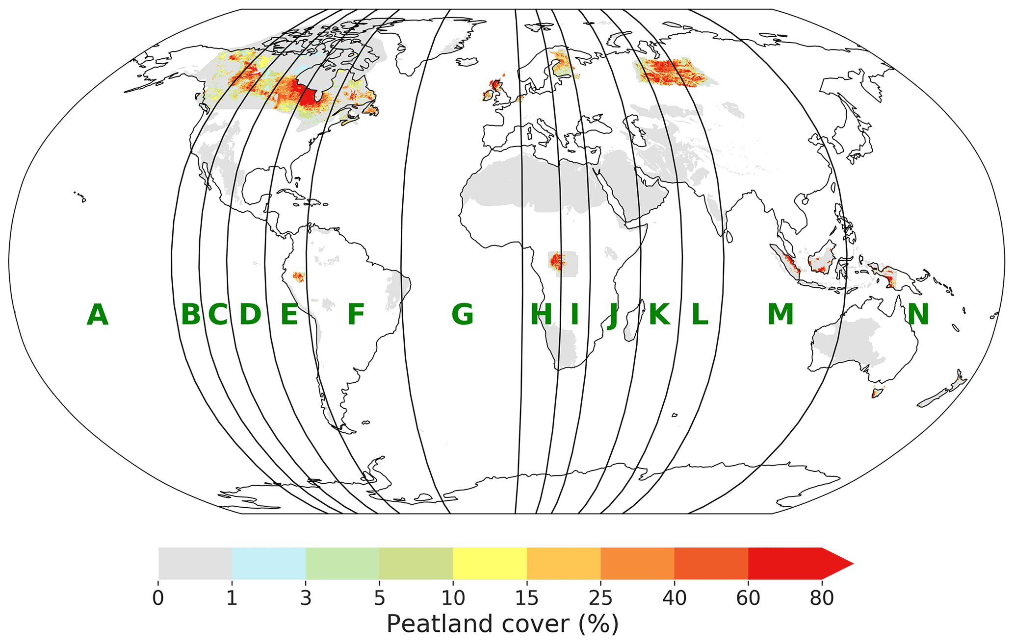
Figure 2Training data for the LightGBM algorithm. Areas in white have no data. The green letters denote the blocks used for the cross-validation scheme. The training block limits were chosen as described in Sect. 2.4.2.
Peatland coverage data for Canada, which has ca. 13 % of the land surface covered with peatlands, comes from Ducks Unlimited Canada (hereafter DUC; Smith et al., 2007) and The Peatlands of Canada database (Tarnocai et al., 2011). Both datasets defined peatlands as wetlands (bogs, fens, swamps, or marshes) with massive deposits of peat at least 40 cm thick, as is the convention in Canada. The Peatlands of Canada database was primarily derived from soil surveys and air photo interpretation. Shapefiles were available with information on bog, fen, and bog–fen features with ≥1 % peat coverage (Tarnocai et al., 2011). The DUC dataset covers the 74.1×10⁴ km2 Boreal Plains region and was derived from a satellite-based remote sensing classification system validated by 5034 field sites (Smith et al., 2007).
The peatlands of the taiga zone of the West Siberian Lowlands (WSL) is estimated by Terentieva et al. (2016) to be 52.4×10⁴ km2, or 4 %–12 % of the global wetland area. To conduct this mapping, Terentieva and co-workers used a supervised classification scheme for Landsat imagery that was trained on field data and high-resolution images from 28 test sites. They estimate their accuracy at 79 % based on 1082 10×10 pixel size validation polygons.
The St. Petersburg region of Russia was mapped by Pflugmacher et al. (2007) using MODIS Nadir bidirectional reflectance distribution function adjusted reflectance (NBAR). The MODIS-NBAR reflectances were combined with empirical regression models to determine sub-pixel peatland coverage. To fit the models, Pflugmacher et al. (2007) drew upon forest inventory data for observed peatland fractional cover over 1105 MODIS pixels with half used for model fitting and half for validation. Error analysis showed good prediction capability with correlation with observations of r=0.92 for unmined peatlands. Pflugmacher et al. (2007) found the region to have approximately 10 % peatland cover.
The Finnish Geologic Survey superficial deposits 1:200 000 map displays peat deposits at 0–30, 30–60, and >60 cm depth (Geological Survey of Finland, 2018). The dataset was created through air photo interpretation and field mapping with the smallest polygon size about 6 ha.
A database for the peatlands of Scotland was recently published by Aitkenhead and Coull (2019). Peatland cover was determined using back-propagation neural networks trained with peatland survey, climate, topography, Landsat imagery, geologic, and land cover data. Aitkenhead and Coull (2019) reports an r2 of 0.67 for peat depth, which we used to determine peatland fractional cover. Peatlands were assumed to have >30 cm peat, and pixels with peat deeper than that were assigned 100 % peatland cover and 0 % elsewhere.
The Derived Irish Peat Map version 2 (DIPMv2) (Connolly and Holden, 2009) was compiled from the land cover and soil maps of Ireland using a rules-based decision tree methodology. Connolly and Holden (2009) estimate the overall accuracy of DIPMv2 to be 85 %. From the DIPMv2, we included raised bogs, low-level Atlantic blanket bogs, and high-level montane blanket bogs in producing a peatland cover map.
Wageningen Environmental Research recently updated the Soil Map of the Netherlands (1:50 000 scale) including peat depth using a combination of boreholes and ordinary kriging (Brouwer et al., 2018; Brouwer and Walvoort, 2019). For each region, a number of boreholes were not used in calibration of the kriging model (roughly 10 %) and retained for evaluation. Based on evaluation against the validation borehole subset, the average peat depth error varied between regions but was commonly between 10 and 20 cm. We used the peat depth to delineate peatland area based on a threshold of 30 cm where thicknesses greater than that were assumed to be 100 % peatland and 0 % elsewhere.
Draper et al. (2014) mapped peatlands for a region of Amazonia in northwestern Peru (the Pastaza-Marañón foreland basin; PMFB). A support vector machine (SVM) classifier was trained with Landsat, ALOS/PALSAR, and Shuttle Radar Topography Mission (SRTM) elevation data. Along with forest census plots and peat thickness measurements, a supervised classification method was used to train the SVM and determine the distribution of peatland vegetation types, as well as above- and below-ground carbon stocks. The three peat-forming vegetation types were pole forest, palm swamp, and open peatlands.
The Cuvette Centrale is located in the central Congo basin. Dargie et al. (2017) used a digital elevation model (DEM) to remove steep slopes and high ground, optical data (Landsat Enhanced Thematic Mapper, ETM+) to identify probable swamp vegetation, which we used as a proxy for peatland fractional coverage, and radar backscatter (L-band synthetic aperture radar; ALOS PALSAR) to identify surface water under forest cover. Together these approaches were used to produce a maximum likelihood tree. They then conducted nine transects of length 2.5 to 20 km to ground truth the data. Most peatlands in this region are located within large interfluvial basins and are largely rain-fed and ombrotrophic. The areal extent of peat in the Cuvette Centrale was estimated to be 14.6×10⁴ km2 (Dargie et al., 2017).
Indonesian peatlands have been mapped by Wetlands International in a series of publications (Wetlands International, 2003, 2004, 2006). The maps have been derived from regional-scale maps and project reports, soil maps, Landsat imagery, and ground truthing. This dataset uses a 30 cm threshold of peat thickness to delineate peatlands.
National maps of New Zealand peatlands were derived from the Fundamental Soil Layers (FSL) soil maps published at 1:50 000 scale by the New Zealand Land Resource Inventory (NZLRI; Landcare Research NZ Ltd, 2000). The polygons in the FSL maps were manually created from aerial photograph analysis with ground truthing. Peatlands were selected by choosing the organic soils class.
Organic soil and peat mapping was undertaken by the Department of Natural Resources and Environment, Tasmania, to provide decision support for fire management and suppression activities in the Tasmanian Wilderness World Heritage Area (Kidd et al., 2021). A DSM approach was used to predict organic soil and peat areas using new and existing soil site data, intersected with a range of environmental predictor datasets, which included vegetation mapping, legacy soil mapping, wetlands, digital elevation models, terrain derivatives, remote sensing (multispectral green or bare areas, gamma radiometrics, Sentinel RADAR), and climate. A binary “presence–absence” calibration set of site data was used to create a digital map index (0–1). Modelling was undertaken using regression trees with 10-fold cross-validation, where spatial output values closer to “1” were deemed to be meeting the environmental conditions conducive to peat formation. The organic soil extent modelling R2 calibration and validation values were 0.77 and 0.70, respectively. Map validation by expert review determined that spatial index values >0.75 were highly likely to be peat (or organic) soils (Kidd et al., 2021).
Peatlands along the Rio Madre de Dios in Peru were mapped by Householder et al. (2012) using Landsat imagery and field observations. They identified 295 peatlands from remote-sensing imagery covering 294 km2 and from 0.1 to 35.0 km2 in size. Field verification was performed at 35 peatlands giving over 800 georeference validation data points.
To increase the number of cells for model training and also improve representation of peatland-free landscapes, we included polygons of ecoregions that should contain little to no peatlands from Olson et al. (2001), thus all areas in these ecoregions and biomes were considered to have zero peatland extent. The ecoregions chosen were the global distribution of the Desert and Xeric Shrublands biome, excluding 15 ecoregions that had a non-zero peatland extent within at least one grid cell according to PEATMAP. This was to ensure we take a conservative approach to the use of these non-peatland masks. Two South American ecoregions (Beni Savanna and the Rio Negro Campinarana; Fig. 2) were also included as peat-free regions. We discuss the inclusion of these ecoregions in Sect. 3.3. A further region of zero peatland extent was defined according to a map of soil organic carbon for the Casanare flooded savannas of Colombia (Martín-López et al., 2022) and expert opinion based upon field observations. We also set peatland area to zero for any pixels that are ice covered as shown in the Global Land Ice Measurements from Space (GLIMS) dataset (GLIMS and NSIDC, 2018).
(Smith et al., 2007)Tarnocai et al. (2011)Terentieva et al. (2016)Pflugmacher et al. (2007)Geological Survey of Finland (2018)Aitkenhead and Coull (2019)Connolly and Holden (2009)Brouwer et al. (2018)Brouwer and Walvoort (2019)Draper et al. (2014)Dargie et al. (2017)Landcare Research NZ Ltd (2000)Kidd et al. (2021)Householder et al. (2012)Table 2Training data (regional peatland mapping products) for the machine learning model.
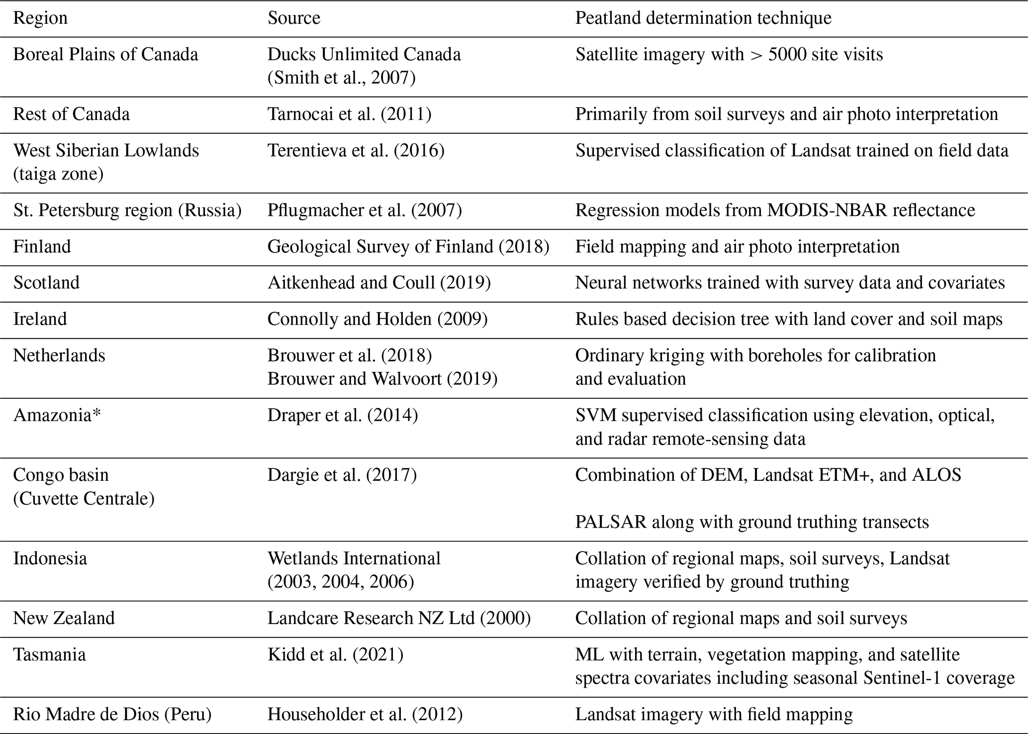
* Pastaza-Marañón foreland basin (PMFB) in northwestern Peru
2.4 Machine learning approach
2.4.1 LightGBM and hyperparameter optimization
The statistical modelling was conducted in the Python programming language (v. 3.8.3). We use a gradient boosting decision tree (GBDT) algorithm called LightGBM (Ke et al., 2017). Decision tree algorithms make iterative splits to partition data according to different criteria. The decision tree will split each node at the feature with the largest information gain, i.e. the most informative. For GBDTs, the information gain is usually measured by the variance after splitting. To avoid issues with overfitting of a decision tree, GBDT algorithms use the boosting technique, which combines multiple decision trees in series to achieve better predictive power as each tree in the series attempts to minimize the errors in the previous tree. The error minimization steps occur through a form of gradient descent in function space where each tree is trained on a residual vector that measures the magnitude and direction of the true target relative to the previous tree (loss function), which successive iterations minimize.
2.4.2 Cross-validation approach
To provide estimates of the error associated with the LightGBM predictions we adopted a blocked-leave-one-out (BLOO) strategy, which is recommended for applications where the predictors could be expected to exhibit spatial autocorrelation (Roberts et al., 2017; Meyer et al., 2019; Ploton et al., 2020). BLOO tends to produce estimates of prediction error that are closer to the “true” error (Roberts et al., 2017), particularly in cases where the sampling strategy is clustered (Rocha et al., 2021). We chose to block our cross-validation (CV) regions based on longitudinal limits to allow both boreal and tropical peatlands to potentially be represented in each block. The optimal number of training blocks is an important determination. Choosing blocks that are too small risks incorrectly increasing our CV-determined model accuracy due to spatial autocorrelation issues, while choosing overly large blocks will result in information loss and worsens our assessed model accuracy unduly. We determine the optimal number of blocks by comparing the length scale of autocorrelation of the model residuals with our block sizes. Figure A1 shows the autocorrelation tends to zero at a length scale (sill) of around 500 km. To accommodate this we set a minimum block size of 10∘ of longitude (which corresponds to roughly 500 km at 65∘ latitude). Based on the constraints of our minimum block size and the need for a roughly even number of training cells in each block, we end up partitioning the globe into 14 blocks as shown in Fig. 2. The CV was performed by holding out one block, training the LightGBM algorithm over the other blocks, and then using that trained model to predict the peatland extent over the held-out block. This was performed for each block in turn and the results averaged to give an estimate of the prediction error.
2.4.3 Predictor selection and model optimization
From the potential peatland covariates listed in Table 1, and discussed in Sect. 2.2.1, we processed 163 global peatland features that could be used by the machine learning model. However, it is likely that many of these predictors will have low predictive power and duplicate information provided by other predictors, leading to over-fitting by the ML algorithm (Dormann et al., 2013). To select only the most relevant features we used both iterative feature removal based on the calculated multicollinearity and recursive feature elimination with cross-validation (RFECV) (Pedregosa et al., 2011), which is a form of backward feature elimination.
Multicollinearity was accounted for by using the calculated variance inflation factor (VIF) to identify and remove highly correlated variables (Alin, 2010). VIF uses ordinary least-squares regression to determine collinearity with the score determined by
where is the multiple coefficient of determination for the feature j on the other features (covariates) defined as the ratio between the sum of squares due to the regression (SSR) and the total sum of squares (SST),
One approach would be to simply set a threshold VIF value and remove all features with VIF values higher than this threshold in a single step. However, in order to avoid the elimination of potentially important features, we chose instead to conduct the exclusion process iteratively. First, each feature had its VIF score calculated. Then all features with a VIF value higher than 5 (corresponding to a of 0.8) were ranked according to their information gain calculated by LightGBM, and the feature with the lowest gain was removed. The model was then retrained and the VIF value recalculated. If features remained that had a VIF above the threshold value, the same ranking and removal would occur until all remaining features had a VIF value below threshold. This step retained 30 features (listed in Table A1). The VIF value chosen is quite stringent, well below what Dormann et al. (2013) suggest as a critical value (10).
We use RFECV with BLOO CV (using the same blocks as described in Sect. 2.4.2) in an iterative manner to ascertain the optimal number of features. RFECV first trains the LightGBM algorithm on the original number of features (here 30) with the features ranked for their importance, based on information gain, for the model's root-mean-square error (RMSE) as determined by the BLOO CV. The least important feature is removed and the model is retrained using the new subset of features. By retraining the model after each feature is held out, we avoid the issue of extrapolation that can occur in permutation-based approaches (as described in Hooker et al., 2021). The algorithm can then produce an estimate of model skill as a function of the number of features trained (Fig. A2). The RFECV algorithm will choose an optimal number of features based on the greatest model skill. Based on Fig. A2, 16 features (highlighted in Table 1) were selected as the optimal number to retain for the optimization process and the final model.
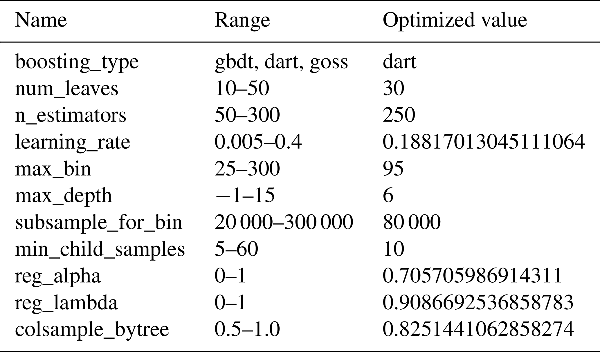
GBDT algorithms tend to require hyperparameter tuning to ensure the model is performing optimally. We employed Bayesian optimization on 11 LightGBM hyperparameters (Table A2) using the hyperopt package (Bergstra et al., 2015) over 500 trials. In each trial, the final 16 predictors identified in the steps above were used in the LightGBM model to optimize the model's calculated RMSE based upon the BLOO CV. The optimized parameters were then used to generate the Peat-ML map.
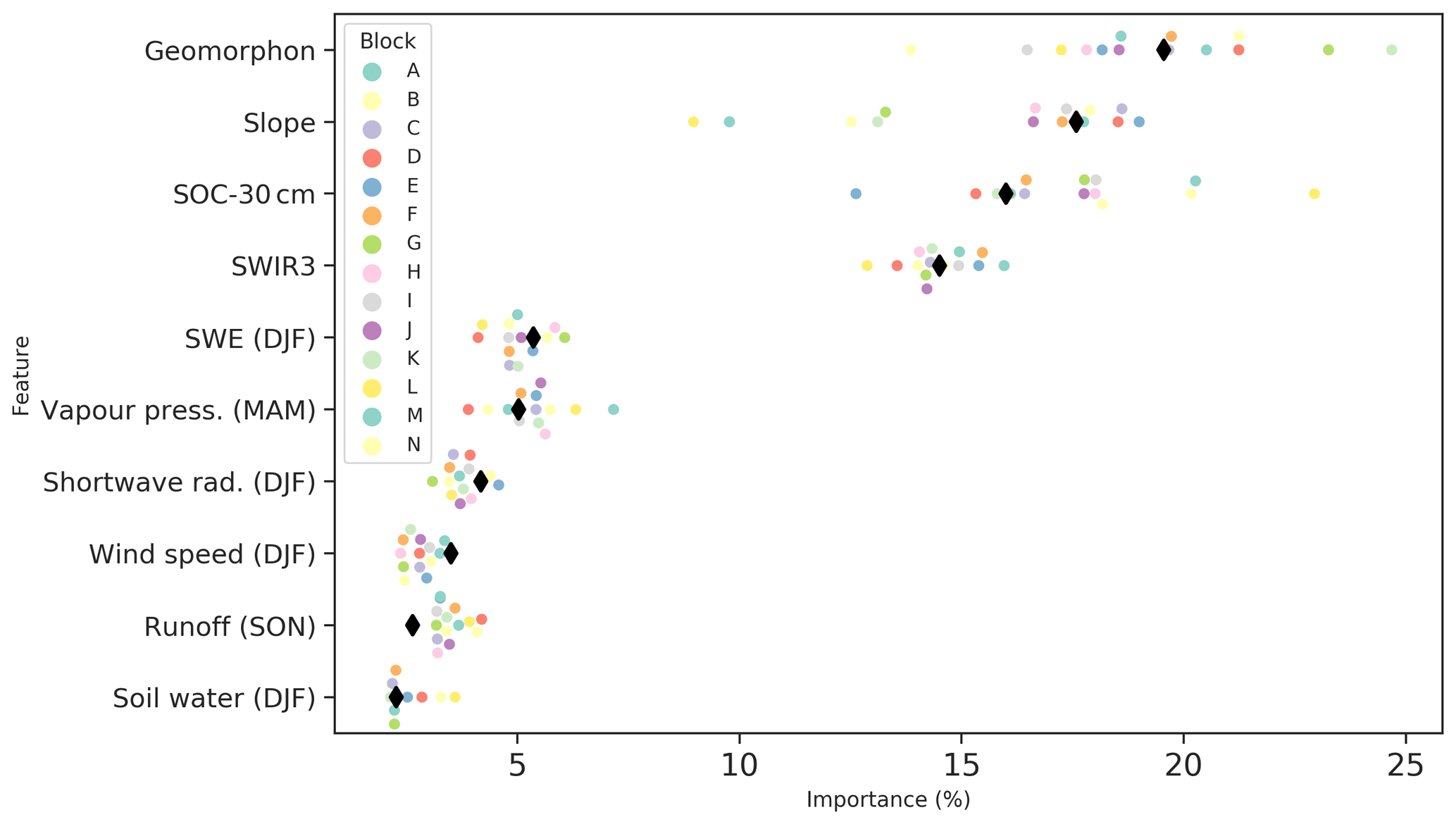
Figure 3Predictor importance based on percent information gain for the top 10 features as determined by the LightGBM algorithm. The feature ranking is shown for each of the blocks used during the BLOO CV (coloured dots; see Sect. 2.4.2). The feature importance from the full model simulation is shown by the black diamonds. SWIR3 is the shortwave infrared radiation reflectance for 2225–2275 nm, geomorphon is the geomorphological landform, SWE is the snow water equivalent, and SOC is soil organic carbon at 30 cm depth. See Table 1 and Sect. 2.2.1 for more details.
3.1 Predictor importance
The top 10 predictors based on information gain as determined by the LightGBM algorithm are shown in Fig. 3. Based on the full LightGBM model runs (hereafter Peat-ML), the most informative feature is the geomorphological landform (e.g. flat, spur, valley, peak), which is calculated using morphometry techniques based on pattern recognition (Amatulli et al., 2020). The next most important predictor is terrain slope, defined as the rate of change in elevation along the direction of the water flow line (Amatulli et al., 2020). The third and fourth most important variables are soil organic carbon at 30 cm depth and shortwave infrared radiation reflectance at 2225–2275 nm (SWIR3). The remaining less important features ( %) relate to climate (DJF snow water equivalent, MAM vapour pressure, DJF shortwave radiation and wind speed, SON runoff, and TerraClimate-derived DJF soil water).
Minasny et al. (2019) suggest the indicators of peatland presence on a regional to global scale are climate data (primarily temperature and precipitation); land use and land cover information; and elevation, slope, and terrain attributes. Slope has also been used in several terrestrial ecosystem models as a means to predict wetland areas; i.e. the flatter a region, the more likely water will stagnate, allowing wetland formation (e.g. Kaplan, 2002; Arora et al., 2018). Interestingly, the top two predictors are important components of the Kaplan (2002) wetland determination scheme. The geomorphological features appear to provide further information about the land surface characteristics that can allow peatland formation distinct from that of slope alone. The importance of the SOC variables demonstrates the close relationship between SOC and peat soils, as has been exploited for peatland mapping in the past (e.g. Hugelius et al., 2020). The importance of SWIR3 likely reflects its utility in determining wet earth from dry earth and providing information about the vegetation water status. SWIR3 is particularly useful as a feature as it can help delineate fens, as otherwise the ML model lacks a predictor of groundwater contributions to surface water, as well as peatlands from uplands in general, as SWIR reflectance is generally sensitive to soil moisture, soil type, and vegetation leaf area index and water content (Wang et al., 2008; Tian and Philpot, 2015). Of the climate predictors, DJF SWE and DJF shortwave radiation could have been used by the ML model to distinguish boreal from tropical peatlands. Vapour pressure may also have some utility in determining peatlands due to the differing evapotranspiration response of peatlands from upland forests (Helbig et al., 2020). In general, however, all the climate variables were of relatively small importance, with roughly 5 % or less importance as measured by information gain.
Figure 3 also shows the feature importance as found by the BLOO CV for each block (whereby each block in the figure shows the feature importance ranking when that block was not trained upon for the CV). Looking at feature importance broken down in this manner reveals some remarkable consistency in some predictors, e.g. relatively low importance predictors (<10 %) remain consistently less important. While other features have highly variable importance principally slope, geomorphon, and SOC-30 cm. These three variables can switch order of importance when trained to exclude certain training blocks during the BLOO CV. When trained with all training data (full model; black diamonds in Fig. 3), predictor importance is generally close to the middle of the range set by the blocks from the BLOO CV, excluding some of the more minor features such as SON runoff or DJF wind speed. This demonstrates that, given there are only 14 blocks, excluding training data as part of the BLOO CV can have relatively large consequences, especially as each peatland region has its own particular characteristics as evidenced by the changing predictor importance. For example, the Cuvette Central, western Amazonia, and tropical islands of Asia all appear to differ significantly regarding characteristics such as peat depth, structure, carbon density, etc. (see Table 1 in Dargie et al., 2017).

3.2 Predicted peatland extents
3.2.1 Global
Global peatland extent as predicted by Peat-ML is shown in Fig. 4. When Peat-ML is compared to PEATMAP (Xu et al., 2018), many major peatlands regions appear similar including Canada, the WSL, the Cuvette Centrale of the Congo, and parts of Scandinavia. However, the two maps also differ substantially. The regions with the most notable difference between the two products include Alaska, parts of Africa excluding the Congo, and eastern Siberia. There are more intermediate peatland extents predicted by Peat-ML, whereas PEATMAP tends to show more regions of 100 % peatland extent with less gradation between peatlands. Our estimated global peatland extent at 4.04×10⁶ km2 is similar to the PEATMAP estimate of 4.23×10⁶ km2 (Table 3).
Gorham (1991)Loisel et al. (2017)Hugelius et al. (2020)Gumbricht et al. (2017)Hugelius et al. (2020)Webster et al. (2018)Table 3Peatland extents as estimated by Peat-ML alongside other literature estimates.
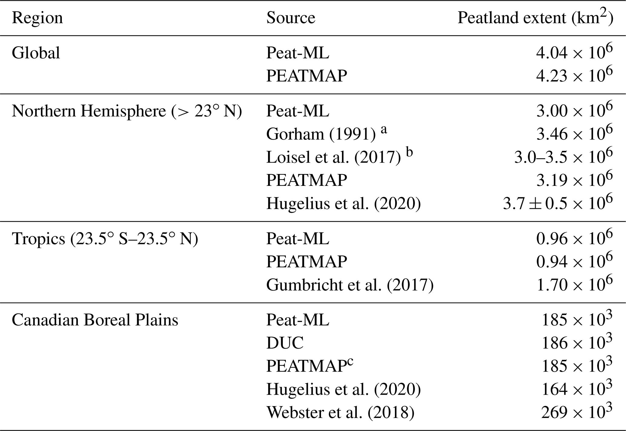
a Boreal and subarctic peatlands. b Suggested best estimate for modern peatland area. Includes a summary of other estimates which range between 2.4 and 4.0×10⁶ km2. c Here PEATMAP's underlying data source is Tarnocai et al. (2011).
Our Northern Hemisphere (>23∘ N) estimates of 3.0 million square kilometres is lower than the other available estimates including PEATMAP (3.2 million square kilometres), the lower bound of Hugelius et al. (2020) (3.2 million square kilometres), and an older estimate of Gorham (1991), but it is at the lower bound suggested by Loisel et al. (2017). In the tropics, our model estimate is roughly the same as PEATMAP but only a little over half of the extent estimated by Gumbricht et al. (2017). The Gumbricht et al. (2017) map was produced through a hybrid approach that uses hydrological modelling, remote-sensing products, hydro-geomorphology from topographic data, and expert assessment. It is only available across the tropics (maximum 40∘ N).
The spatial distribution of the predicted peatlands will now be examined in detail. We focus on regions that have either multiple other peatland mapping products for comparison or contain large areas of predicted peatlands.
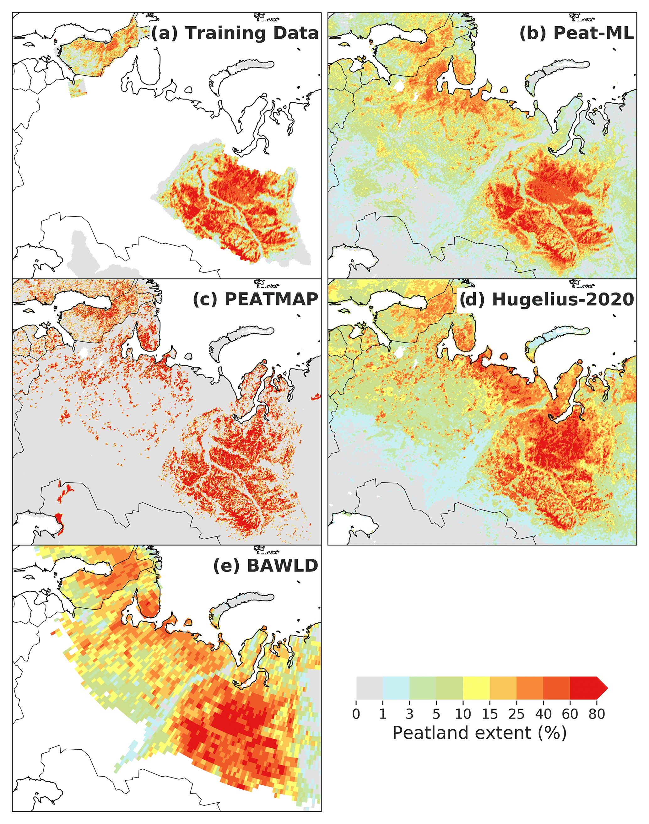
Figure 5Maps of eastern European and Russian peatlands including (a) training data used by the ML model; (b) Peat-ML-predicted peatlands; and the peatland coverage from (c) PEATMAP (Xu et al., 2018), (d) Hugelius et al. (2020), and (e) the Boreal–Arctic Wetland and Lake Dataset (BAWLD; Olefeldt et al., 2021).
3.2.2 Boreal peatlands: Europe and Russia
Figure 5 shows the peatland extent in the WSL, western Russia, and parts of Scandinavia for Peat-ML, its training data, PEATMAP, Hugelius et al. (2020), and the Boreal–Arctic Wetland and Lake Dataset (BAWLD) (Olefeldt et al., 2021). The Hugelius et al. (2020) dataset is derived from the mean of two soil datasets and is only available for the Northern Hemisphere (>23∘ N). The BAWLD product is derived from expert assessment that is then extrapolated through the use of random forest models and geospatial datasets across the boreal and Arctic regions. The original spatial resolution is relatively coarse at 1∘ by 1∘. For the WSL region, all four products are similar, with only slight differences in the peatland fractional cover (rather than its spatial distribution). Peat-ML shows strong similarity with its training data as would be expected. PEATMAP stands out compared to the other maps due to its almost binary peatland coverage showing either high values or no peatlands with little gradation in between. Compared to Hugelius et al. (2020), Peat-ML shows less peatlands in the northern edge of the Northwestern region of Russia but more by the White Sea. Both PEATMAP and Peat-ML do not show peatlands near the mouth of the Kara River to the northwest of the terminus of the Ural Mountains, as evident in Hugelius et al. (2020) and BAWLD, while Peat-ML and BAWLD show few peatlands on the Yamal Peninsula, where both PEATMAP and Hugelius et al. (2020) suggest appreciable extents. Generally, Peat-ML has more similarity to PEATMAP than Hugelius et al. (2020) and BAWLD over the western Russian domain.
All maps show relatively similar distributions of peatlands surrounding the Baltic Sea (Fig. 5). None of the maps indicate peatlands by the Caspian Sea as seen in PEATMAP, except some small extents (1 %–3 % predicted by Peat-ML) to the northwest of those depicted in PEATMAP.
As with Eastern Europe, Western Europe is similar in that PEATMAP shows a more binary representation of the peatland extent compared to the other maps (Fig. A5). Peat-ML and Hugelius et al. (2020) have fairly similar peatland distributions and extents. The main differences are expressed in small pockets of peatlands, e.g. eastern Spain has scattered peatlands in Hugelius et al. (2020) that are not found in Peat-ML or PEATMAP, whereas in western Hungary both Hugelius et al. (2020) and PEATMAP show small peatlands not predicted to be as extensive by Peat-ML.
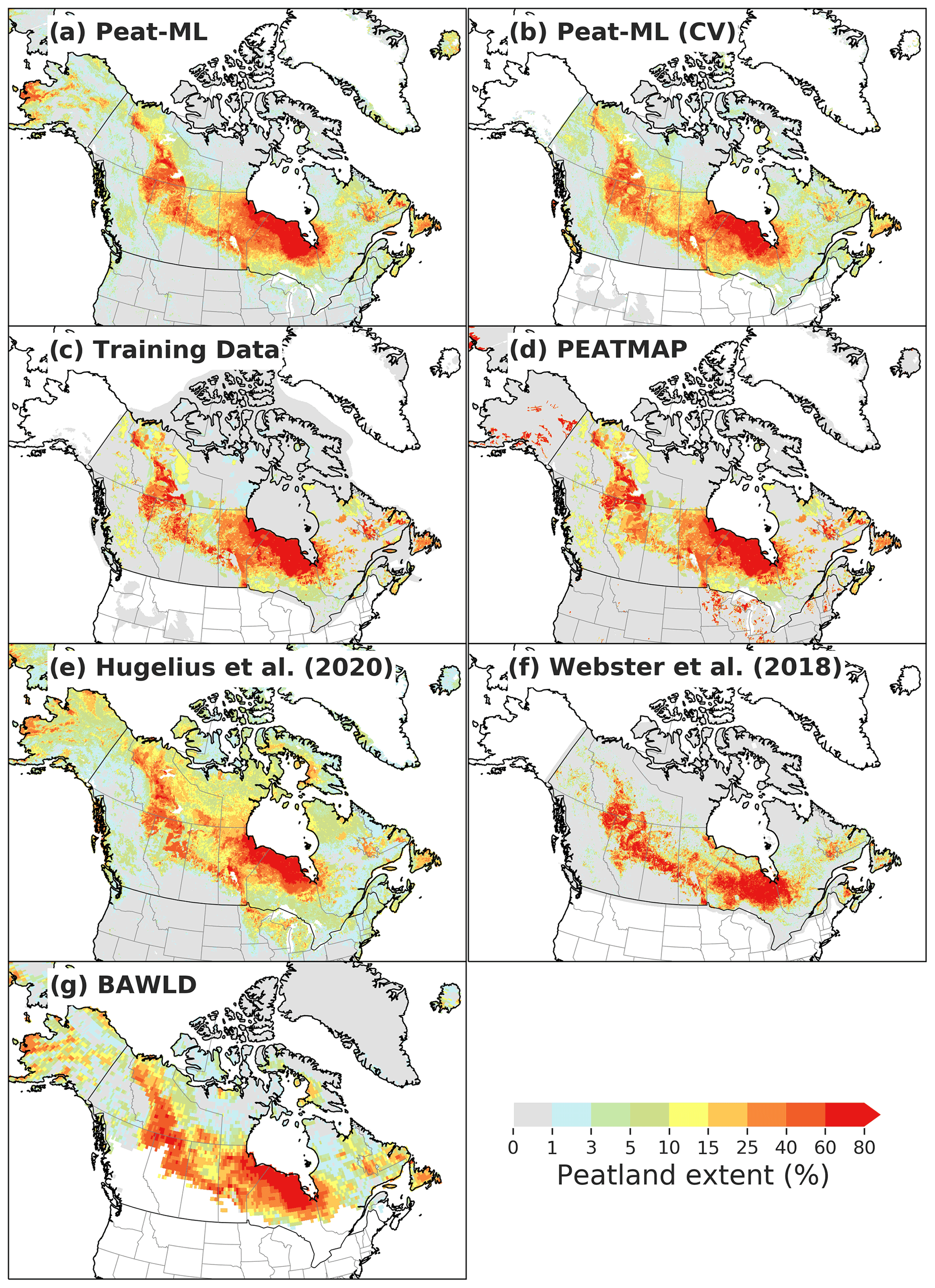
Figure 6Peatland extents for Canada, the northern contiguous USA, and Alaska for (a) Peat-ML, (b) Peat-ML from the BLOO CV, (c) the training data used for the ML model, and four other peatland extent products (d–f).
3.2.3 Boreal peatlands: Canada and Alaska
For the northern contiguous USA, for Canada, and for Alaska, peatlands extents are shown in Fig. 6. Alaskan peatlands predicted by Peat-ML have some similarity to the Hugelius et al. (2020) map and BAWLD, with extensive peatlands in western Alaska (Lower Yukon region). These peatlands are not evident in PEATMAP, which shows less extensive but high-coverage peatlands along the southern and eastern edges of the state. Peat-ML, Hugelius et al. (2020), and BAWLD predict peatlands along the Alaska North Slope that are not evident with PEATMAP. Other reports suggest extensive wetlands in Alaska (e.g. Glass, 1992), but we are not aware of any mapping product detailing peatland-specific coverage.
For Peat-ML, the Canadian peatlands from Tarnocai et al. (2011) and DUC (Smith et al., 2007) are used as training data, which naturally gives good correspondence between Fig. 6a and c. For a more informative comparison of the general model skill for boreal peatland regions, Peat-ML predictions from the BLOO CV simulation are also shown, as this would give some indication of predictions without the benefit of training upon a particular region's peatlands (Fig. 6b). Generally, all datasets shown in Fig. 6 display some strong similarities, with large peatlands shown for the Hudson's Bay Lowlands (HBL), the Mackenzie Delta, and across the Boreal Plains, yet important differences are also visible. Webster et al. (2018) shows little peatland along the southern edge of the Hudson's Bay, perhaps due to their peatland determination model's emphasis on treed peatlands. Webster et al. (2018) also show generally higher peatland coverage where peatlands are present than the other datasets. Hugelius et al. (2020) predicts extensive but relatively low coverage across much of the Canadian eastern Arctic that is not found in any of the other peatland maps. Of the five peatland maps, the most closely corresponding peatland extents appear to be between PEATMAP, BAWLD, and Peat-ML.
The northern USA has some peatlands around the Great Lakes evident in PEATMAP and Hugelius et al. (2020) (∼10 %–60 %), which are also predicted but appear less extensive in Peat-ML (usually ∼1 %–15 %). Besides the coverage differences, the products have a similar spatial extent, although PEATMAP's peatlands are more commonly higher coverage per identified peatland.
3.2.4 Tropical peatlands: South America and Central America
South American peatlands are shown in Fig. 7. Peat-ML peatland training data for this region (Fig. 7a) are currently limited, encompassing only Peru's Pastaza-Marañón foreland basin (PMFB) and the Rio Madre de Dios. In early simulations with Peat-ML and maps from other modelling processes (e.g. Gumbricht et al., 2017), we noticed predictions for high peatland coverage in areas of South America where peat is not known to occur. This includes seasonally flooded savannas, such as the Llanos de Moxos (Beni Savanna) and Llanos Orientales of Colombia and Venezuela. A recent field expedition searching for peat in the Colombian Llanos failed to discover any peat deposits (Martín-López et al., 2022), which could indicate that these tropical savanna biomes are generally not able to form extensive peat deposits. Additionally, white sand ecosystems are not known to support extensive peatlands, and thus we also excluded the Rio Negro Campinarana ecoregion that corresponds with white sandy soils (Spodosols/Podzols) and not Histosols. Without these negative data, we would likely overpredict peat extent in South America rather severely.
Peat-ML predicts an extensive peatland in the PMFB and central Amazonia. The extent of peatlands in this region is lower than in PEATMAP, mainly due the generally lower extent per grid cell, despite being in broadly similar regions. Both PEATMAP and Peat-ML show peatlands along the northeastern coast of the continent. Peat-ML predicts smaller peatland extents (generally <10 %–15 % coverage) in the Pantanal and along the Paraguay River as it joins the Paraná River down to the Rio de la Plata, which are not evident in PEATMAP.
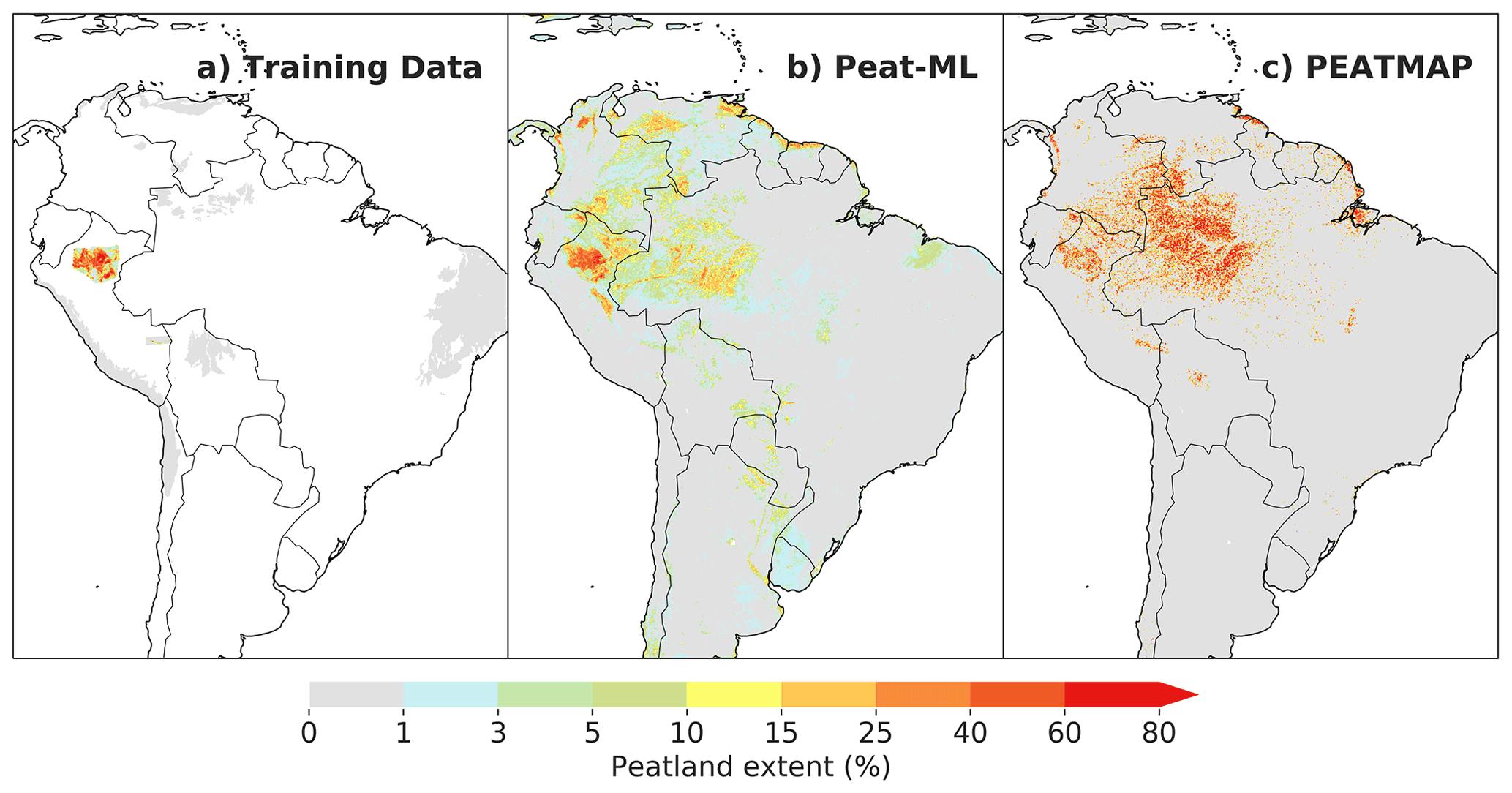
Figure 7South American peatland extents. Panel (a) shows Peat-ML training data, panel (b) shows Peat-ML-predicted peatland coverage, and panel (c) shows PEATMAP (Xu et al., 2018), which is taken from Gumbricht et al. (2017) for this region.
There are some non-peatland river floodplains that Peat-ML characterizes as peatlands, such as Colombia's Rio Guaviare. This river may be too dynamic to allow extensive peat formation due to relatively rapid meandering that would scour away peat-forming depressions faster than the organic matter can accumulate or else bury potential peat with mineral sediments from the Andes (Junk, 1982). Given the lack of an appropriate predictor for these hydro-geomorphological processes operating on decadal to centennial timescales, it is not surprising that Peat-ML may overestimate peat extent in these ecosystems. Other areas, like Colombia's Amazon catchment region, might be susceptible to similar processes as these regions are suggested to be floodplain forests in Ricaurte et al. (2017); however, their map is based on the CORINE Land Cover data for Colombia (IDEAM, 2010). Other areas in Colombia where Peat-ML predicts peatlands include parts of the Orinoco catchment region, where Ricaurte et al. (2017) shows flooded grassland savannas and riparian wetlands, and the Caribbean catchment region, where peatlands are indicated by CORINE with other wetland types. Given that the CORINE land cover product is based upon remote sensing with little ground truthing, it is possible that several of these wetland regions shown in Ricaurte et al. (2017) are actually peat-forming regions, making it difficult to definitively evaluate Peat-ML against this dataset. Besides the occasional small peatland area (e.g. in the Páramo of Ecuador; Hribljan et al., 2017), there are few sources of high-quality peatland mapping products for South America to evaluate Peat-ML against. While Peru has the PMFB mapped by Draper et al. (2014) and the Rio Madre de Dios by Householder et al. (2012) and is proposed to have extensive peatlands by Gumbricht et al. (2017) and Peat-ML, there is presently no national peatland inventory (López Gonzales et al., 2020).
Peat-ML predicts more peatland extent than PEATMAP in Central America (Fig. A6). Much of the predicted peatlands are close to coastlines, in particular along the Atlantic coasts of Mexico, Nicaragua, Costa Rica, and Cuba. Peat-ML places more extensive peatlands on the Yucatán Peninsula of Mexico, which is not evident in PEATMAP. A desk-based assessment of peatlands based upon cartographic approaches with solicited expert assessment shows similar distributions of peatland extent, but with less peatlands in the Yucatán (Peters and Tegetmeyer, 2019). The Yucatán peninsula has relatively extensive marsh and mangrove coastal wetlands but is a karstic landscape with a highly permeable carbonate substrate (Adame et al., 2013) suggesting Peat-ML is overestimating peat extent for the inland portions of the peninsula.
3.2.5 Tropical peatlands: Africa and the Indonesian Archipelago
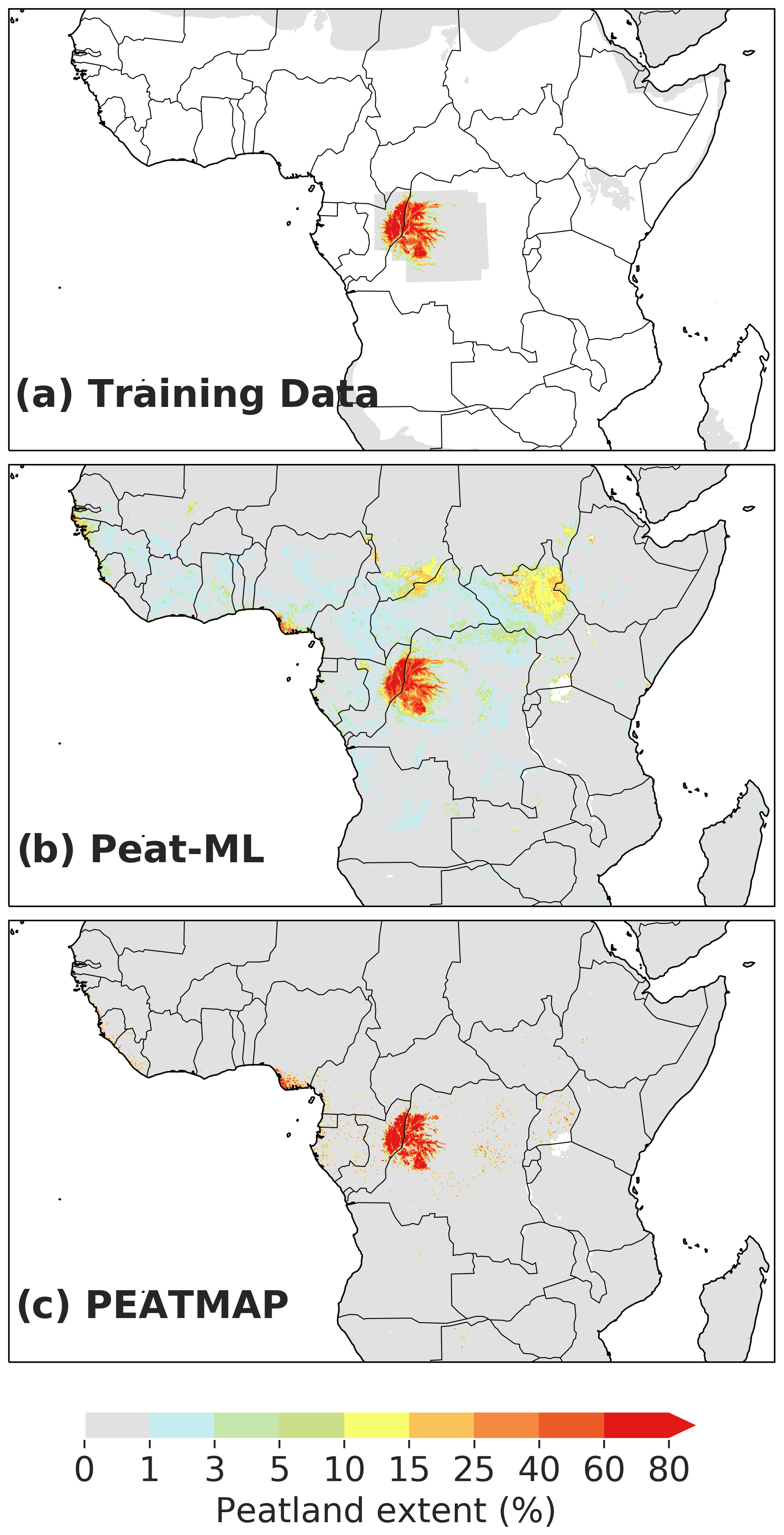
African peatlands (Fig. 8) are also poorly mapped, making it difficult to evaluate the Peat-ML results. There are notable differences between Peat-ML and PEATMAP. PEATMAP shows very few peatlands outside the Congo's Cuvette Centrale, whereas Peat-ML has relatively extensive peatlands in South Sudan along the border of the Central African Republic and Chad. This is in general agreement with more qualitative African peatland extent estimates (Grundling and Grootjans, 2016) and demonstrates Peat-ML's ability to reasonably determine peatland extents in regions where reliable spatially explicit mapping products are absent. Regardless, Peat-ML may still be underestimating African peatlands due to a lack of appropriate training data. An example is the newly documented peatlands in the Okavango Delta (Gelinas, 2018), which have a dominantly herbaceous vegetation cover (sedges, papyrus, grasses), while our only training dataset for Africa is a swamp forest (Cuvette Centrale). Future iterations of Peat-ML may profit from some active mapping campaigns presently underway in East Africa (Alexandra Barthalmes, personal communication, 2021) that could provide much needed training data and thereby improve predictions for the peatland regions of Africa. Improving understanding of African peatland extents will likely remain challenging; however, due to land use pressures that may complicate peatland identification and mapping as suggested by Grundling and Grootjans (2016), African peatlands are heavily utilized by rural populations that depend on the peatland's water and organic soils for crop cultivation.
While much of the Indonesian Archipelago contains training data for the ML algorithm, the neighbouring states of Papua New Guinea, Brunei, and Malaysia are entirely model-predicted areas (Fig. A7). While Malaysian peatlands appear similar between Peat-ML and PEATMAP, Papua New Guinea is quite different. PEATMAP shows extensive peatlands in the central mountainous region of the country, while Peat-ML has the peatlands placed in the surrounding lowland regions. There is some indication that the mountainous regions should have extensive peatlands (Hope, 2015). These peatland complexes appear to be sufficiently different from the Peat-ML training data that the ML model is unable to predict them.
3.3 Model quality estimation
Besides the qualitative discussion above, we estimated the quality of our predicted peatland extent through two different approaches. First, we compared our model results against the training data detailed in Sect. 2.3. For this analysis, we performed a BLOO CV as described in Sect. 2.4.2. Peat-ML (CV) accuracy had an r2 of 0.72, a mean bias error (MBE) of −0.29 %, and an RMSE of 9.11 % (Fig. 9b). The model performance across each of the 12 training blocks can be seen in Figs. A3 and A4. While the mean r2 across all training blocks was 0.72, it ranged from a low of 0.20 (predicting for block F in the BLOO CV in Fig. 2) to a high of 0.88 (block E). One caveat of our error estimation presented here is that we are computing it based upon the datasets used for model training. If these datasets themselves have errors or omissions, as would be expected, then this will diminish the accuracy of our error estimation, as well as the quality of the ML model itself, since they form the benchmark that Peat-ML is compared against.
Peat-ML likely underestimates peatland coverage, as can be seen from its negative MBE (also visible in the regression line shown in Fig. 9). We hypothesize that this low bias may stem from the use of biomes and ecoregions to denote peatland-free areas. It is possible, since these regions are fairly coarsely defined, that we may be inadvertently assigning small-scale, niche peatland areas as non-peatlands (although we take measures to avoid this; see Sect. 2.3). If that is the case, we would be training the model to miss the characteristics of these more niche peatland environments and biassing our results. We use the ecoregions and biomes from Olson et al. (2001) to delineate these non-peatland regions to counter the fact that high-quality peatland datasets are typically created only for peatland-rich regions. Without inclusion of this peatland-poor training data, we would be providing the algorithm only peatland-rich training data, leaving the model poorly trained for peatland-poor regions. Machine learning algorithms are best suited to interpolation problems (e.g. McCartney et al., 2020), and thus it is best to produce training data that give the full range of conditions under which the model is expected to produce predictions. Additionally, for the peatlands of South America, we found that we were overpredicting peatland extents as determined by expert opinion and field observation, primarily due to the paucity of high-quality peatland maps from the continent. As more high-quality peatland mapping products become available from presently poorly mapped regions, the use of these ecoregions and biomes could be removed or reduced.

Figure 9Scatterplots of Peat-ML-predicted peatland cover versus actual peatland cover (from the datasets listed in Table 2) for the full model (a) and as determined by the BLOO CV (b).
The second approach to estimate the quality of our peatland map focuses on the Boreal Plains (BP) region of Canada, where we have several peatland products for comparison (Fig. A8). The DUC remote-sensing-based dataset for this region is uniquely well ground truthed, with over 5000 site visits over its 74.1×10⁴ km2 area. The DUC dataset has a peatland extent of 186×103 km2 (Table 3) for the BP region, which is about the same as PEATMAP (whose underlying data source in this region is Tarnocai et al. (2011)). Peat-ML (CV) estimates 199×103 km2 (this is derived from the BLOO CV simulations to allow a more fair comparison; it is 185×103 km2 when estimated by the full model, i.e. Peat-ML) while Hugelius et al. (2020) estimates 164×103 km2 and Webster et al. (2018) estimates 269×103 km2. We can estimate a confidence interval using the Peat-ML (CV) RMSE, which gives a range of 140×103 to 234×103 km2. This range suggests that the predicted extent is only significantly different between Peat-ML (CV) and Webster et al. (2018). Given its quality, we take the DUC dataset as our benchmark and use it to determine the accuracy of Peat-ML and other products (Table 4). As expected, Peat-ML compares well with the DUC dataset, as it is trained using that dataset. A more useful comparison is with Peat-ML (CV), where the model is not trained with the DUC dataset. Peat-ML (CV) has the second lowest RMSE, mean bias, and explained variance scores after Tarnocai et al. (2011) in all instances (Table 4). For the DUC region, the Peat-ML (CV) results indicate a higher predictive performance than a peatland mapping product based on soil databases (Hugelius et al., 2020); another based on boosted regression trees using forest structure maps, bioclimatic variables, and surface slopes (Webster et al., 2018); and one based upon ML models informed by expert assessment, although BAWLD has the lowest spatial resolution, which may have impeded its performance against the high-resolution DUC dataset. Peat-ML (CV) is, however, outperformed by a more traditional and labour-intensive product based on air-photo interpretation and soil surveys (Tarnocai et al., 2011), although the performance difference is relatively small (e.g. RMSE difference of 0.39 %). This indicates that our model, for this region at least, is of similar or higher quality compared to other peatland mapping products available from a diverse range of methodologies.
Hugelius et al. (2020)Webster et al. (2018)Olefeldt et al. (2021)Table 4Statistical comparison of peatland map products as evaluated against the DUC dataset (Smith et al., 2007). RMSE is the root-mean-square error. The explained variance score (calculated as , where y is the observations, is the prediction, and σ is the standard deviation) has a best possible value of 1.0, with lower scores indicating worse performance.
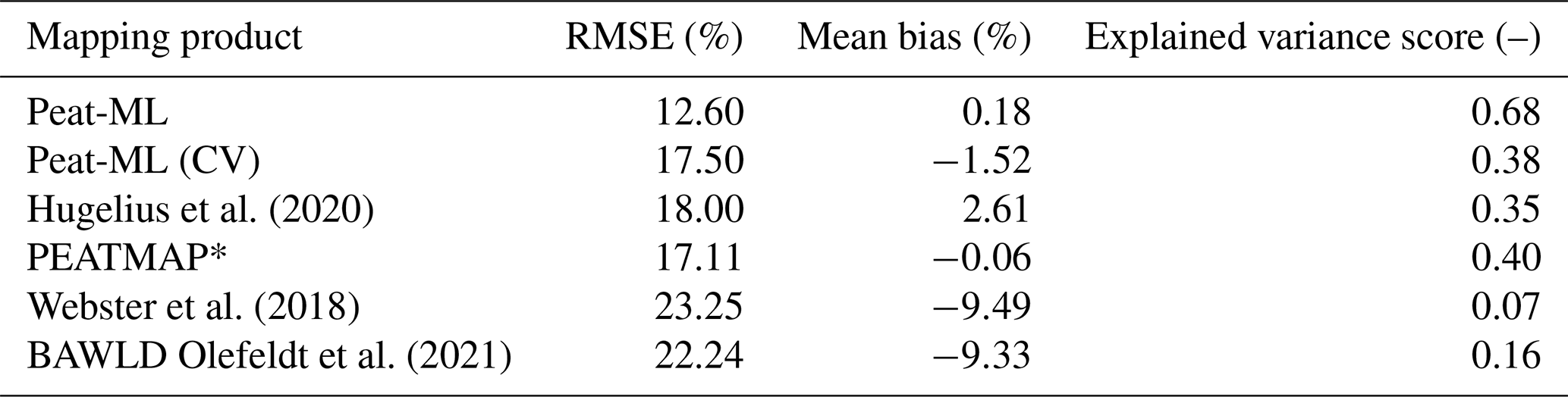
* Tarnocai et al. (2011) is the underlying data source for PEATMAP in the DUC domain
3.4 Limitations of our approach
The purpose of our study is to produce a map of peatland distribution for use as an input geophysical field for ESMs with integrated peatland models. It is tempting to ask whether our technique can give any insights into peat formation or the conditions necessary for a peatland to develop and persist. While our approach is not prescriptive like Hugelius et al. (2020), where peatlands are defined based upon the soil carbon at a location, it is challenging to derive causal information from our simulations. Many of the top features determined by the LightGBM algorithm (Fig. 3) are related to geomorphological characteristics, soil carbon, vegetation and soil water status, and climate. However, peatlands themselves will alter the environment they form within (e.g. fill in depressions with peat or alter the hydrologic balance for the vegetation), and thus it is difficult to differentiate cause from effect.
A weakness of our approach lies in the availability of training data. Our training data for peatland distribution are generally biased towards the high latitudes. While we have good coverage of peatland presence in Canada and western Siberia (see Sect. 2.2), we presently lack extensive high-quality peatland distribution maps for much of the Southern Hemisphere and tropics. However, we expect new products to become available over time (e.g. Anda et al., 2021; Bourgeau-Chavez et al., 2021). As one of our main predictors is sensitive to vegetation (SWIR3), there is also the possibility that peatland types that are not represented in our training data (e.g. mangroves and marshes in the neotropics or papyrus marshes of Africa) will be poorly represented by the available training data that the ML algorithm uses to derive a relationship between the vegetation-based predictor and peatland extent. An additional challenge is the importance of seasonality of covariates (e.g. climate, vegetation indices) that differ significantly between the tropics and high latitudes based on their local dynamics. This may be addressed in future versions of Peat-ML by training separate models for both regions alongside predictors tailored to the dynamics of each region, although that depends on a greatly increasing availability of tropical training datasets to ensure well-trained models.
In addition, as discussed in Sect. 3.3, it would be beneficial to include mapping products for regions where peatlands are relatively sparse. As our peatland sampling strategy was determined by the availability of high-quality peatland maps, we were not able to choose systematic (Rocha et al., 2021) or feature-based sampling strategies that could be more optimal for peatland prediction. Our approach would also benefit from greater availability of processed, global-scale products that should be sensitive to water status below the peat surface like L-band synthetic aperture radar (e.g. Touzi et al., 2013).
We present a new global peatland fractional coverage map, Peat-ML, at a scale of 5 arcmin resolution. Peat-ML was generated using machine learning techniques drawing upon drivers of peatland formation that include spatially distributed climate, soil, geomorphology, and vegetation data. The ML model was trained using maps of peatland fractional coverage for 14 relatively extensive regions along with masks of non-peatland areas. To evaluate Peat-ML, we qualitatively compared it to other available peatland maps, and we also quantified model performance using two approaches. The first approach is based on a blocked leave-one-out cross-validation strategy designed to minimize the influence of spatial autocorrelation. Based upon that approach, Peat-ML has an average r2 of 0.73 with a root-mean-square error and mean bias error of 9.11 % and −0.36 %, respectively, when evaluated against our model training data. Our second model quality estimate was generated by comparing Peat-ML against a high-quality, extensively ground-truthed map for the 74.1×10⁴ km2 Canadian Boreal Plains region. This comparison suggests Peat-ML is of comparable or higher quality than other presently available peatland mapping products. Future versions of Peat-ML would benefit from further high-quality and ground-truthed datasets of peatland extent, especially in tropical regions.
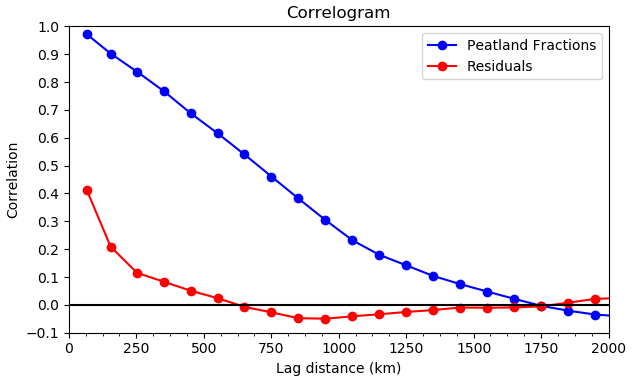
Figure A1Correlogram showing the spatial correlation between model residuals as a function of distance computed using Moran's I.
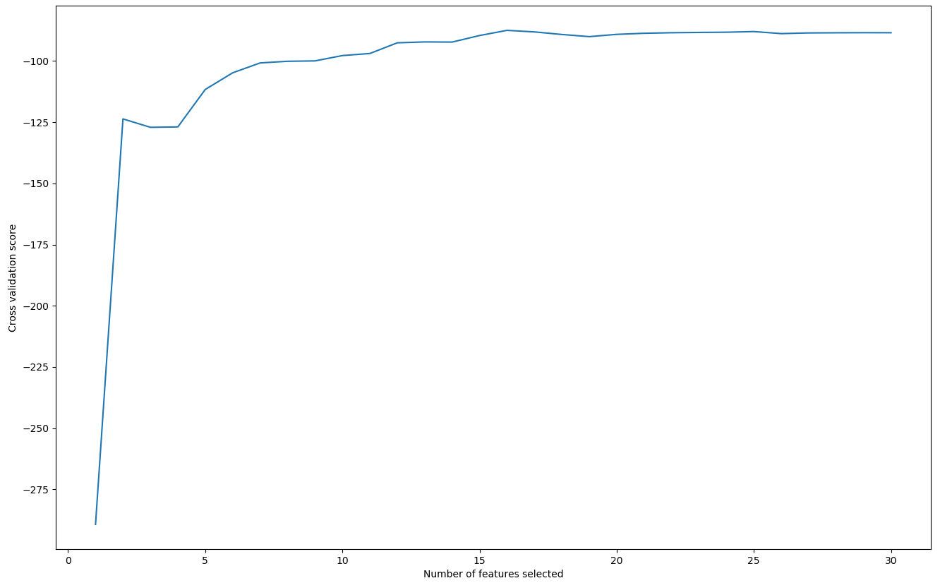
Figure A2Cross-validation scores against the number of features selected by RFECV (see Sect. 2.4.3).
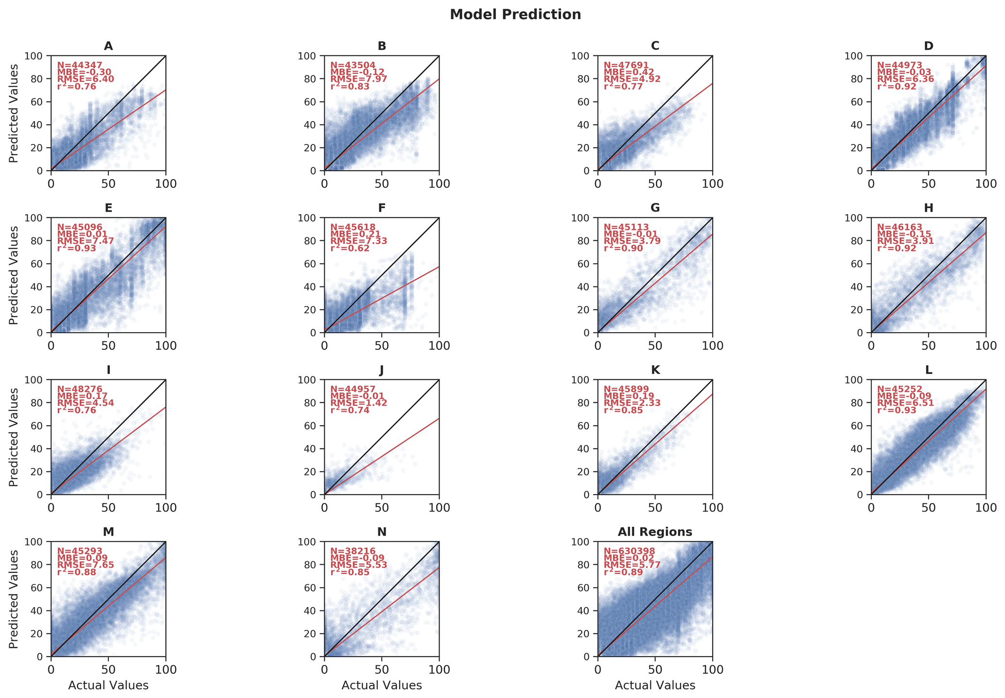
Figure A3Scatterplots of full model Peat-ML-predicted peatland extent and peatland extent from the peatland training datasets over the 14 BLOO CV blocks.
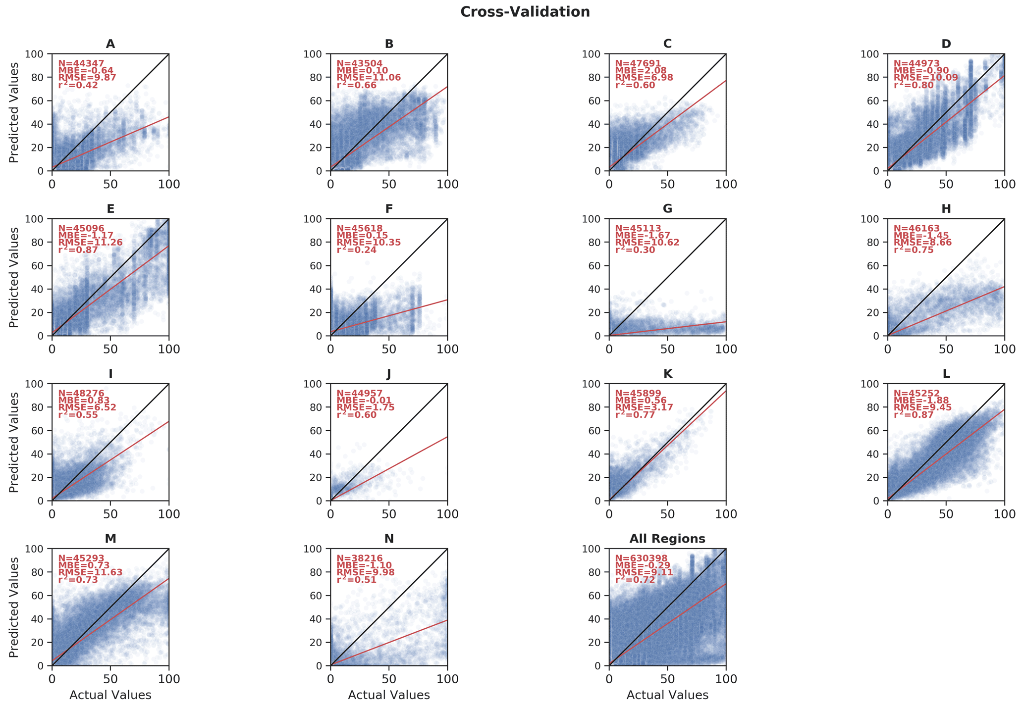
Figure A4Scatterplots of the CV trials for Peat-ML (Peat-ML CV)-predicted peatland extent and peatland extent from the peatland training datasets over the 14 BLOO CV blocks.

Figure A5Maps of western European peatlands, including (a) training data used by the ML model; (b) Peat-ML-predicted peatlands; and the peatland coverage from (c) PEATMAP (Xu et al., 2018), (d) Hugelius et al. (2020), and (e) BAWLD (Olefeldt et al., 2021), whose domain only partly extends over the region displayed.
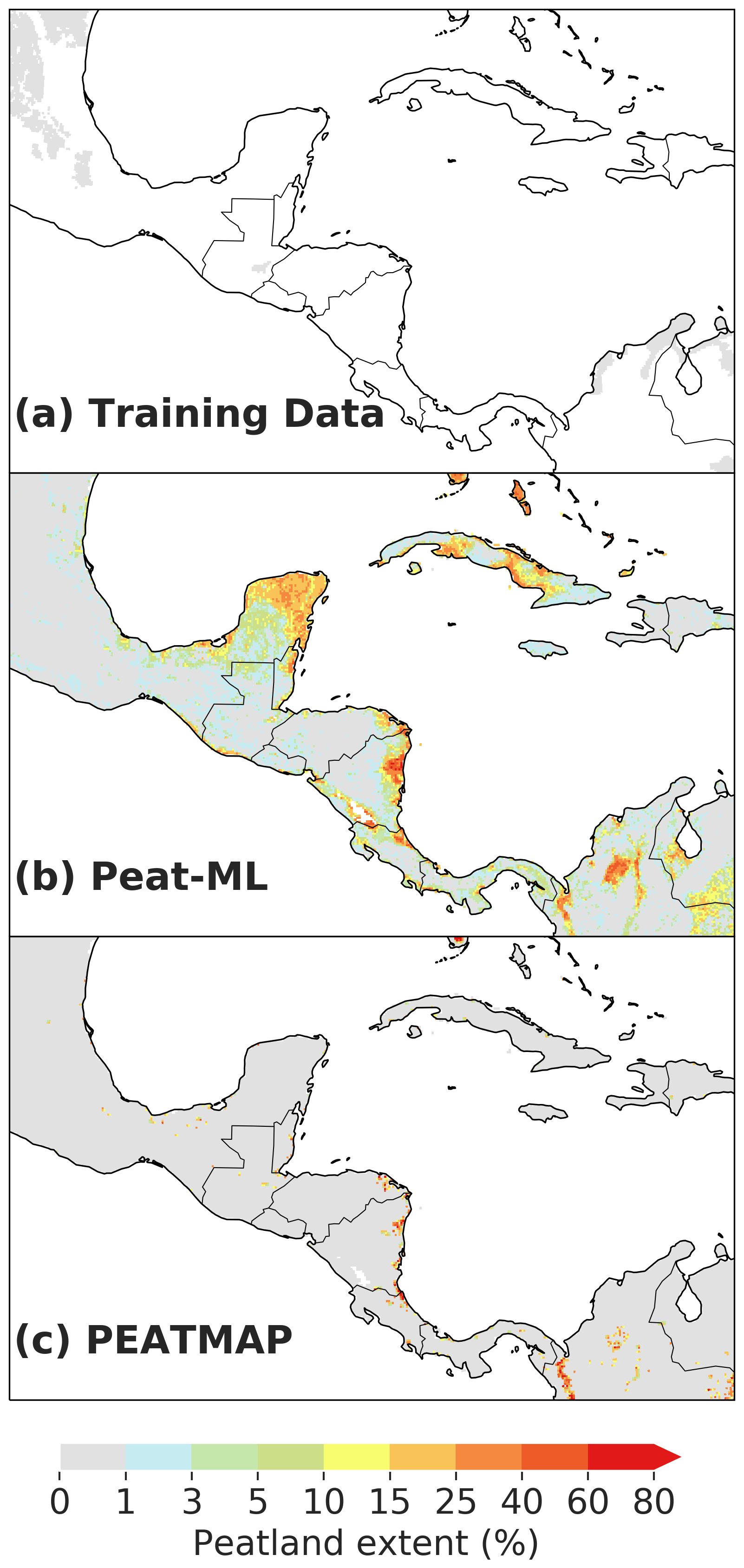
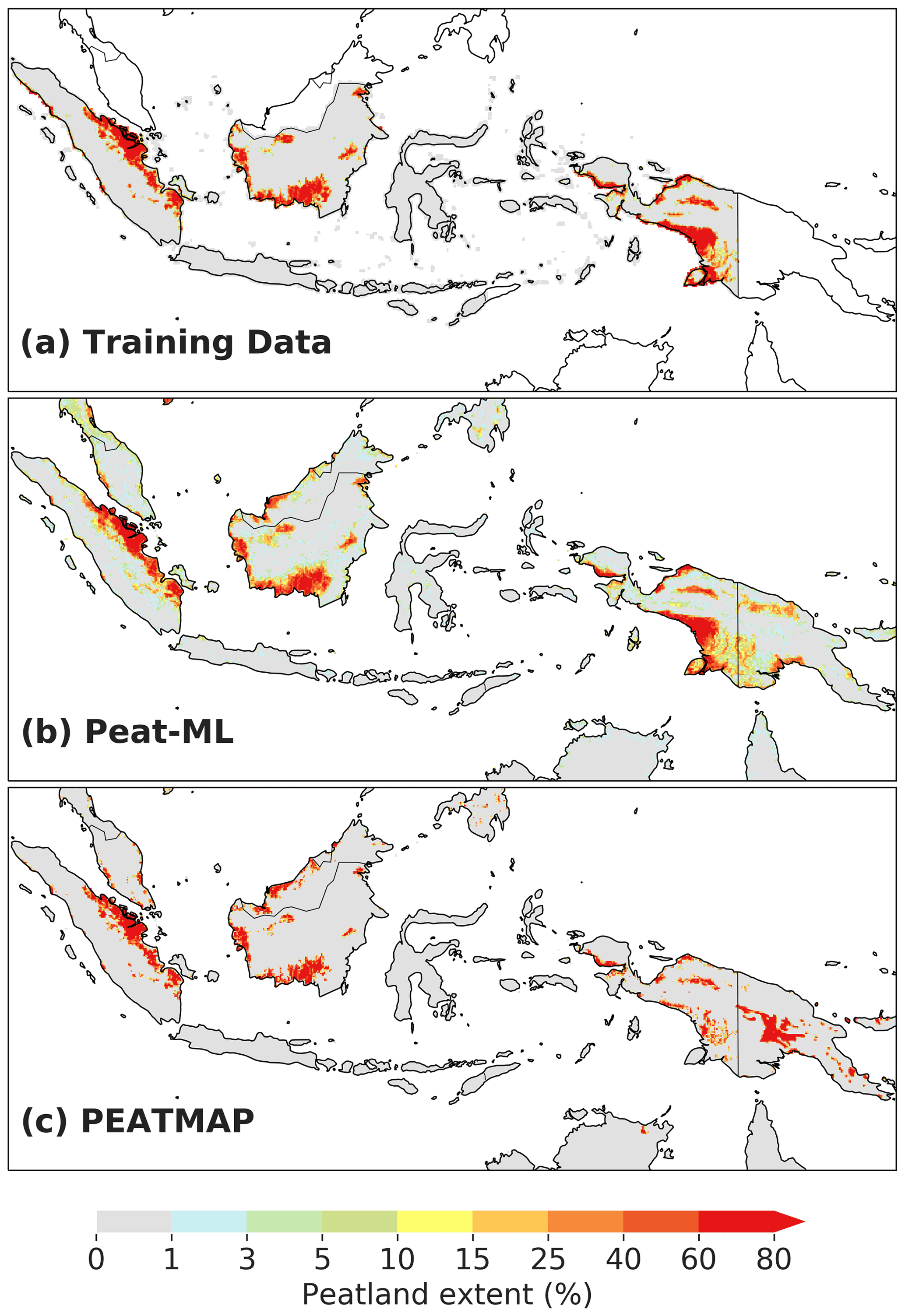
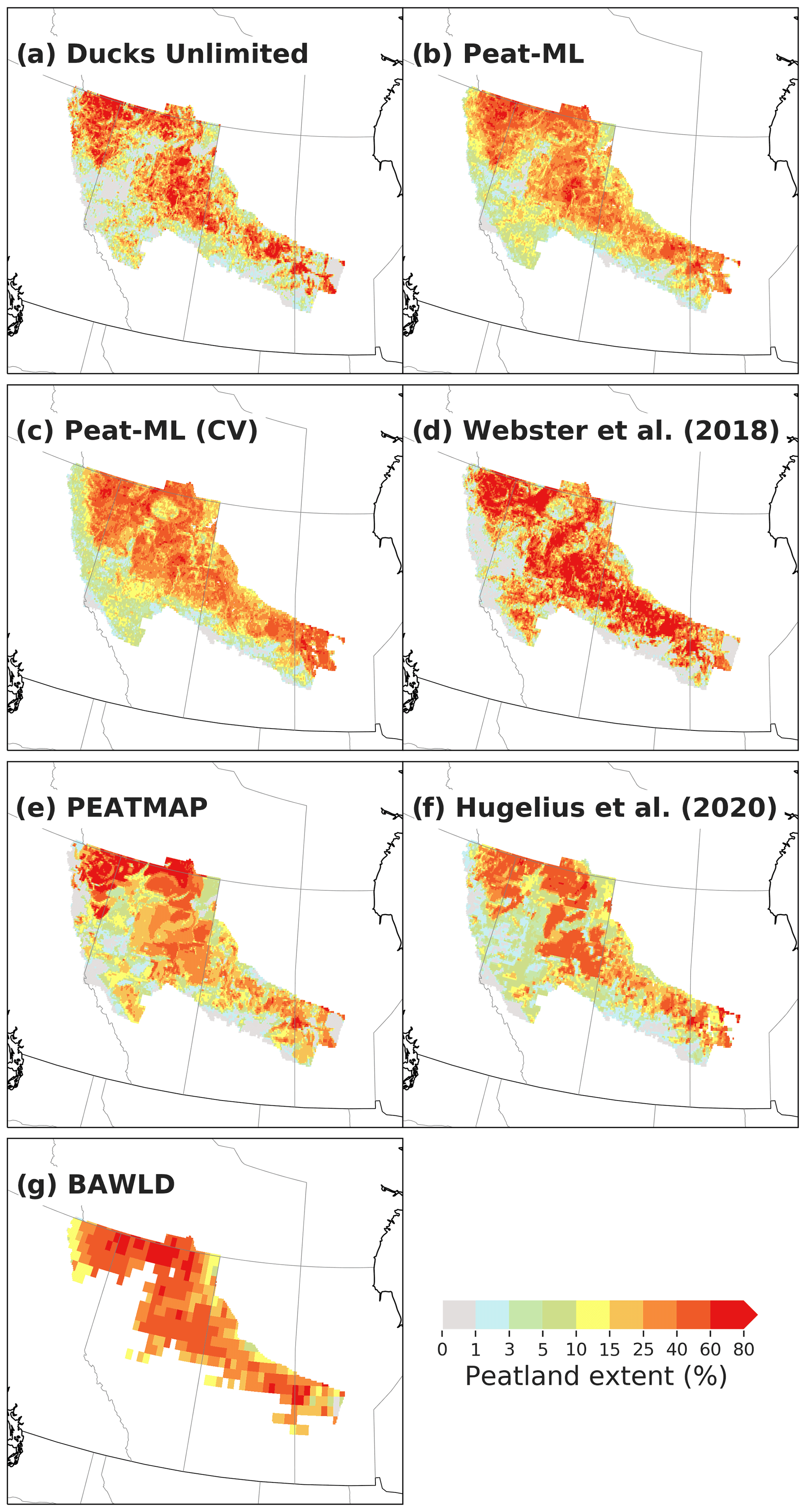
Figure A8Maps of peatland extent for the Boreal Plains of Canada.
Table A1The 30 predictors selected using VIF with a threshold value of 5. The final 16 features that were further selected by the RFECV algorithm for use in the final model are listed in Table 1. See Sect. 2.2.1 for further discussion on the variable processing.
a The means of DJF, MAM ,JJA, and SON refer to the 3-month periods indicated by the first letter of each month, respectively. b 2225–2275 nm. c Product between the upstream catchment area and the tangent of the local slope angle. d Measures the rate of change perpendicular to the slope gradient and is related to the convergence and divergence of flow across a surface. e The rate of change of the elevation in a specific direction. f The rate of change of the slope in a predetermined direction. g Terrain variable that details the convergent areas as channels and divergent areas as ridges. It has a value of −100 for ridges, 0 for planar or flat areas, and up to 100 for sink areas. h Angular direction that a slope faces. i Calculated from sine of the slope multiplied by the cosine. Northness gives a continuous measure of the orientation combined with the slope. For the Northern Hemisphere, a northness approaching 1 gives a northern exposure on a vertical slope (that is a slope exposed to a very low amount of solar radiation), conversely a northness of −1 gives a very steep southern slope that would be highly exposed to solar radiation.
Table A2LightGBM hyperparameters that underwent Bayesian optimization and their final optimized values. See Sect. 2.2.1 for further discussion on the variable processing. See Pedregosa et al. (2011) documentation for further discussion about each hyperparameter.
Python code for the statistical modelling is available at https://doi.org/10.5281/zenodo.6345309 (Melton et al., 2022). A netCDF format version of the Peat-ML dataset is available at https://doi.org/10.5281/zenodo.5794336 (Melton et al., 2021).
JRM conceptualized the study. EC, JRM, and MF performed data curation, formal analysis, investigation, and software and methodology development. JMML, RSW, and KM also contributed to methodology development. KM, JMML, HCQ, and DK provided resources. JRM and EC did the visualization. Validation was done by RSW, JMML, HCQ, LVV, DK, EC, and JRM. JRM wrote the original draft of the manuscript. All authors reviewed and edited the final manuscript.
The contact author has declared that neither they nor their co-authors have any competing interests.
Publisher's note: Copernicus Publications remains neutral with regard to jurisdictional claims in published maps and institutional affiliations.
We acknowledge the efforts of Yuanqiao Wu and Diana Verseghy, who led an earlier effort to predict global peatland extents using machine learning approaches. We thank Dirk Flugmacher, Matt Aitkenhead, Fokke Brouwer, Freddie Draper, Greta Dargie, and Rudiyanto for sharing their peatland mapping products. We also thank Camila Delgado-Montes for processing the Rio Madre de Dios data. We have adopted the colour bar scheme from Hugelius et al. (2020) for our peatland extent plots. Lastly, we thank Michel Bechtold for comments about an earlier study that we used to improve the design of this study.
This paper was edited by David Lawrence and reviewed by two anonymous referees.
Abatzoglou, J. T., Dobrowski, S. Z., Parks, S. A., and Hegewisch, K. C.: TerraClimate, a high-resolution global dataset of monthly climate and climatic water balance from 1958–2015, Sci. Data, 5, 170191, https://doi.org/10.1038/sdata.2017.191, 2018. a, b, c, d
Adame, M. F., Kauffman, J. B., Medina, I., Gamboa, J. N., Torres, O., Caamal, J. P., Reza, M., and Herrera-Silveira, J. A.: Carbon stocks of tropical coastal wetlands within the karstic landscape of the Mexican Caribbean, PLoS One, 8, e56569, https://doi.org/10.1371/journal.pone.0056569, 2013. a
Aitkenhead, M. J. and Coull, M. C.: Mapping soil profile depth, bulk density and carbon stock in Scotland using remote sensing and spatial covariates, Eur. J. Soil Sci., https://doi.org/10.1111/ejss.12916, 2019. a, b, c
Alin, A.: Multicollinearity, Wiley Interdiscip. Rev. Comput. Stat., 2, 370–374, https://doi.org/10.1002/wics.84, 2010. a
Amatulli, G., McInerney, D., Sethi, T., Strobl, P., and Domisch, S.: Geomorpho90m, empirical evaluation and accuracy assessment of global high-resolution geomorphometric layers, Sci. Data, 7, 162, https://doi.org/10.1038/s41597-020-0479-6, 2020. a, b, c, d, e, f
Anda, M., Ritung, S., Suryani, E., Sukarman, Hikmat, M., Yatno, E., Mulyani, A., Subandiono, R. E., Suratman, and Husnain: Revisiting tropical peatlands in Indonesia: Semi-detailed mapping, extent and depth distribution assessment, Geoderma, 402, 115235, https://doi.org/10.1016/j.geoderma.2021.115235, 2021. a
Arora, V. K., Melton, J. R., and Plummer, D.: An assessment of natural methane fluxes simulated by the CLASS-CTEM model, Biogeosciences, 15, 4683–4709, https://doi.org/10.5194/bg-15-4683-2018, 2018. a
Bechtold, M., De Lannoy, G. J. M., Koster, R. D., Reichle, R. H., Mahanama, S. P., Bleuten, W., Bourgault, M. A., Brümmer, C., Burdun, I., Desai, A. R., Devito, K., Grünwald, T., Grygoruk, M., Humphreys, E. R., Klatt, J., Kurbatova, J., Lohila, A., Munir, T. M., Nilsson, M. B., Price, J. S., Röhl, M., Schneider, A., and Tiemeyer, B.: PEAT–CLSM: A Specific Treatment of Peatland Hydrology in the NASA Catchment Land Surface Model, J. Adv. Model. Earth Sy., 11, 2130–2162, https://doi.org/10.1029/2018MS001574, 2019. a
Bergstra, J., Komer, B., Eliasmith, C., Yamins, D., and Cox, D. D.: Hyperopt: a Python library for model selection and hyperparameter optimization, Comput. Sci. Discov., 8, 014008, https://doi.org/10.1088/1749-4699/8/1/014008, 2015. a
Beven, K. J. and Kirkby, M. J.: A physically based, variable contributing area model of basin hydrology, Hydrol. Sci. Bull., 24, 43–69, https://doi.org/10.1080/02626667909491834, 1979. a
Bohn, T. J., Melton, J. R., Ito, A., Kleinen, T., Spahni, R., Stocker, B. D., Zhang, B., Zhu, X., Schroeder, R., Glagolev, M. V., Maksyutov, S., Brovkin, V., Chen, G., Denisov, S. N., Eliseev, A. V., Gallego-Sala, A., McDonald, K. C., Rawlins, M. A., Riley, W. J., Subin, Z. M., Tian, H., Zhuang, Q., and Kaplan, J. O.: WETCHIMP-WSL: intercomparison of wetland methane emissions models over West Siberia, Biogeosciences, 12, 3321–3349, https://doi.org/10.5194/bg-12-3321-2015, 2015. a
Bourgeau-Chavez, L. L., Grelik, S. L., Battaglia, M. J., Leisman, D. J., Chimner, R. A., Hribljan, J. A., Lilleskov, E. A., Draper, F. C., Zutta, B. R., Hergoualc'h, K., Bhomia, R. K., and Lähteenoja, O.: Advances in Amazonian Peatland Discrimination With Multi-Temporal PALSAR Refines Estimates of Peatland Distribution, C Stocks and Deforestation, Front. Earth Sci. Chin., 9, 1019, https://doi.org/10.3389/feart.2021.676748, 2021. a
Brouwer, F. and Walvoort, D. J. J.: Basisregistratie Ondergrond (BRO) – actualisatie bodemkaart : Herkartering van de bodem in Eemland, Tech. Rep. 2352-2739, Wettelijke Onderzoekstaken Natuur & Milieu, Wageningen, 2019. a, b
Brouwer, F., Vries, F. D., and Walvoort, D. J. J.: Basisregistratie Ondergrond (BRO) actualisatie bodemkaart : Herkartering van de bodem in Flevoland, Tech. Rep. 2352-2739, Wettelijke Onderzoekstaken Natuur & Milieu, Wageningen, 2018. a, b
Connolly, J. and Holden, N. M.: Mapping peat soils in Ireland: updating the derived Irish peat map, Ir. Geogr., 42, 343–352, https://doi.org/10.1080/00750770903407989, 2009. a, b, c
Dargie, G. C., Lewis, S. L., Lawson, I. T., Mitchard, E. T. A., Page, S. E., Bocko, Y. E., and Ifo, S. A.: Age, extent and carbon storage of the central Congo Basin peatland complex, Nature, 542, 86–90, https://doi.org/10.1038/nature21048, 2017. a, b, c, d
Didan, K. and Barreto, A.: VIIRS/NPP Vegetation Indices 16-Day L3 Global 500m SIN Grid V001, USGS, https://doi.org/10.5067/VIIRS/VNP13A1.001, 2018. a, b
Dormann, C. F., Elith, J., Bacher, S., Buchmann, C., Carl, G., Carré, G., Marquéz, J. R. G., Gruber, B., Lafourcade, B., Leitão, P. J., Münkemüller, T., McClean, C., Osborne, P. E., Reineking, B., Schröder, B., Skidmore, A. K., Zurell, D., and Lautenbach, S.: Collinearity: a review of methods to deal with it and a simulation study evaluating their performance, Ecography, 36, 27–46, https://doi.org/10.1111/j.1600-0587.2012.07348.x, 2013. a, b
Draper, F. C., Roucoux, K. H., Lawson, I. T., Mitchard, E. T. A., Coronado, E. N. H., Lähteenoja, O., Montenegro, L. T., Sandoval, E. V., Zaráte, R., and Baker, T. R.: The distribution and amount of carbon in the largest peatland complex in Amazonia, Environ. Res. Lett., 9, 124017, https://doi.org/10.1088/1748-9326/9/12/124017, 2014. a, b, c
Friedl, M., Gray, J., and Sulla-Menashe, D.: MCD12Q2 MODIS/Terra+Aqua Land Cover Dynamics Yearly L3 Global 500m SIN Grid V006, https://doi.org/10.5067/MODIS/MCD12Q2.006 (last access: 4 September 2020), 2019. a, b, c
GDAL/OGR contributors: GDAL/OGR Geospatial Data Abstraction software Library, Open Source Geospatial Foundation, https://gdal.org (last access: 28 December 2020), 2021. a
Gelinas, N.: Into the Okavango, USA, https://www.nationalgeographic.org/projects/okavango/ (last access: 11 October 2021), 2018. a
Geological Survey of Finland: Superficial deposits of Finland 1:200 000 (sediment polygons) v.10.1, 2018. a, b
Glass, R. L.: Alaska Wetland Resources, Tech. Rep. 2425, U.S. Geological Survey, Water-Supply Paper 2425, 1992. a
GLIMS and NSIDC: Global Land Ice Measurements from Space glacier database. Compiled and made available by the international GLIMS community and the National Snow and Ice Data Center, Boulder CO, USA, https://doi.org/10.7265/N5V98602 (last access: 4 March 2021), 2018. a
Gorelick, N., Hancher, M., Dixon, M., Ilyushchenko, S., Thau, D., and Moore, R.: Google Earth Engine: Planetary-scale geospatial analysis for everyone, Remote Sens. Environ., 202, 18–27, https://doi.org/10.1016/j.rse.2017.06.031, 2017. a
Gorham, E.: Northern Peatlands: Role in the Carbon Cycle and Probable Responses to Climatic Warming, Ecol. Appl., 1, 182–195, https://doi.org/10.2307/1941811, 1991. a, b
Grundling, P. and Grootjans, A. P.: Peatlands of Africa, in: The Wetland Book: II: Distribution, Description and Conservation, edited by: Finlayson, C. M., Milton, G. R., Prentice, R. C., and Davidson, N. C., Springer Netherlands, Dordrecht, 1–10, https://doi.org/10.1007/978-94-007-6173-5_112-1, 2016. a, b
Gumbricht, T., Roman-Cuesta, R. M., Verchot, L., Herold, M., Wittmann, F., Householder, E., Herold, N., and Murdiyarso, D.: An expert system model for mapping tropical wetlands and peatlands reveals South America as the largest contributor, Glob. Chang. Biol., 23, 3581–3599, https://doi.org/10.1111/gcb.13689, 2017. a, b, c, d, e, f, g, h
Harris, I., Osborn, T. J., Jones, P., and Lister, D.: Version 4 of the CRU TS monthly high-resolution gridded multivariate climate dataset, Sci. Data, 7, 109, https://doi.org/10.1038/s41597-020-0453-3, 2020. a
Helbig, M., Waddington, J. M., Alekseychik, P., Amiro, B. D., Aurela, M., Barr, A. G., Black, T. A., Blanken, P. D., Carey, S. K., Chen, J., Chi, J., Desai, A. R., Dunn, A., Euskirchen, E. S., Flanagan, L. B., Forbrich, I., Friborg, T., Grelle, A., Harder, S., Heliasz, M., Humphreys, E. R., Ikawa, H., Isabelle, P.-E., Iwata, H., Jassal, R., Korkiakoski, M., Kurbatova, J., Kutzbach, L., Lindroth, A., Löfvenius, M. O., Lohila, A., Mammarella, I., Marsh, P., Maximov, T., Melton, J. R., Moore, P. A., Nadeau, D. F., Nicholls, E. M., Nilsson, M. B., Ohta, T., Peichl, M., Petrone, R. M., Petrov, R., Prokushkin, A., Quinton, W. L., Reed, D. E., Roulet, N. T., Runkle, B. R. K., Sonnentag, O., Strachan, I. B., Taillardat, P., Tuittila, E.-S., Tuovinen, J.-P., Turner, J., Ueyama, M., Varlagin, A., Wilmking, M., Wofsy, S. C., and Zyrianov, V.: Increasing contribution of peatlands to boreal evapotranspiration in a warming climate, Nat. Clim. Chang., 10, 555–560, https://doi.org/10.1038/s41558-020-0763-7, 2020. a
Hengl, T.: Soil property layers from openlandmap.org. All data are available under the Open Data Commons Open Database License (ODbL) and/or Creative Commons Attribution-ShareAlike 4.0 International license (CC BY-SA), https://doi.org/10.5281/zenodo.2525663 (last access: 4 September 2020), 2018. a, b, c
Hengl, T. and MacMillan, R. A.: Predictive Soil Mapping with R, Lulu.com, 2019. a
Hooker, G., Mentch, L., and Zhou, S.: Unrestricted Permutation forces Extrapolation: Variable Importance Requires at least One More Model, or There Is No Free Variable Importance, arXiv: 1905.03151 (stat.ME), 2021. a
Hope, G. S.: Peat in the mountains of new guinea, Mires Peat, 15, 1–21, 2015. a
Householder, J. E., Janovec, J. P., Tobler, M. W., Page, S., and Lähteenoja, O.: Peatlands of the Madre de Dios River of Peru: distribution, geomorphology, and habitat diversity, Wetlands, 32, 359–368, 2012. a, b, c
Hribljan, J. A., Suarez, E., Bourgeau-Chavez, L., Endres, S., Lilleskov, E. A., Chimbolema, S., Wayson, C., Serocki, E., and Chimner, R. A.: Multidate, multisensor remote sensing reveals high density of carbon-rich mountain peatlands in the páramo of Ecuador, Glob. Chang. Biol., 23, 5412–5425, https://doi.org/10.1111/gcb.13807, 2017. a
Huete, A., Didan, K., Miura, T., Rodriguez, E. P., Gao, X., and Ferreira, L. G.: Overview of the radiometric and biophysical performance of the MODIS vegetation indices, Remote Sens. Environ., 83, 195–213, https://doi.org/10.1016/S0034-4257(02)00096-2, 2002. a
Hugelius, G., Loisel, J., Chadburn, S., Jackson, R. B., Jones, M., MacDonald, G., Marushchak, M., Olefeldt, D., Packalen, M., Siewert, M. B., Treat, C., Turetsky, M., Voigt, C., and Yu, Z.: Large stocks of peatland carbon and nitrogen are vulnerable to permafrost thaw, P. Natl. Acad. Sci. USA, 117, 20438–20446, https://doi.org/10.1073/pnas.1916387117, 2020. a, b, c, d, e, f, g, h, i, j, k, l, m, n, o, p, q, r, s, t, u, v, w, x, y
IDEAM: Leyenda nacional de coberturas de la tierra: metodología CORINE Land Cover adaptada para Colombia: Escala 1:100 000, edited by: Martínez Ardila, N. J. and Murcia García, U. G., Ministerio De Ambiente, Vivienda Y Desarrollo Territorial Instituto De Hidrología, Meteorología Y Estudios Ambientales – IDEAM, ISBN 978-958-806729-2, 2010. a
Izumi, Y., Widodo, J., Kausarian, H., Demirci, S., Takahashi, A., Razi, P., Nasucha, M., Yang, H., and Tetuko S. S., J.: Potential of soil moisture retrieval for tropical peatlands in Indonesia using ALOS-2 L-band full-polarimetric SAR data, Int. J. Remote Sens., 40, 5938–5956, https://doi.org/10.1080/01431161.2019.1584927, 2019. a
Jackson, R. B., Lajtha, K., Crow, S. E., Hugelius, G., Kramer, M. G., and Piñeiro, G.: The Ecology of Soil Carbon: Pools, Vulnerabilities, and Biotic and Abiotic Controls, Annu. Rev. Ecol. Evol. S., 48, 419–445, https://doi.org/10.1146/annurev-ecolsys-112414-054234, 2017. a
Joosten, H. and Clarke, D.: Wise use of mires and peatlands, International Mire Conservation Group and International Peat Society, ISBN 951-97744-8-3, 304, 2002. a, b
Junk, W. J.: Amazonian flood plains: their ecology, present and potential use, Revue d'Hydrobiologie Tropicale, 15, 285–301, 1982. a
Kaplan, J. O.: Wetlands at the Last Glacial Maximum: Distribution and methane emissions, Geophys. Res. Lett., 29, 3-1–3-4, https://doi.org/10.1029/2001GL013366, 2002. a, b
Ke, G., Meng, Q., Finley, T., Wang, T., Chen, W., Ma, W., Ye, Q., and Liu, T.-Y.: LightGBM: A Highly Efficient Gradient Boosting Decision Tree, in: Advances in Neural Information Processing Systems 30, edited by: Guyon, I., Luxburg, U. V., Bengio, S., Wallach, H., Fergus, R., Vishwanathan, S., and Garnett, R., 3146–3154, Curran Associates, Inc., 2017. a
Kidd, D., Moreton, R., and Brown, G.: Tasmanian Organic Soil Mapping Project, Methods Report. Nature Conservation Report 21/2, unpublished report, 2021. a, b, c
Kobayashi, S., Ota, Y., Harada, Y., Ebita, A., Moriya, M., Onoda, H., Onogi, K., Kamahori, H., Kobayashi, C., Endo, H., Miyaoka, K., and Takahashi, K.: The JRA-55 Reanalysis: General Specifications and Basic Characteristics, J. Meteorol. Soc. JPN, 93, 5–48, https://doi.org/10.2151/jmsj.2015-001, 2015. a
Krankina, O. N., Pflugmacher, D., Friedl, M., Cohen, W. B., Nelson, P., and Baccini, A.: Meeting the challenge of mapping peatlands with remotely sensed data, Biogeosciences, 5, 1809–1820, https://doi.org/10.5194/bg-5-1809-2008, 2008. a
Köchy, M., Hiederer, R., and Freibauer, A.: Global distribution of soil organic carbon – Part 1: Masses and frequency distributions of SOC stocks for the tropics, permafrost regions, wetlands, and the world, SOIL, 1, 351–365, https://doi.org/10.5194/soil-1-351-2015, 2015. a
Lähteenoja, O. and Roucoux, K.: Inception, history and development of peatlands in the Amazon Basin, PAGES News, 18, 27–28, https://doi.org/10.22498/pages.18.1.27, 2010. a
Landcare Research NZ Ltd: Fundamental Soil Layer – New Zealand Soil Classification, https://doi.org/10.7931/L10T0 (last access: 4 January 2020), 2000. a, b
Largeron, C., Krinner, G., Ciais, P., and Brutel-Vuilmet, C.: Implementing northern peatlands in a global land surface model: description and evaluation in the ORCHIDEE high-latitude version model (ORC-HL-PEAT), Geosci. Model Dev., 11, 3279–3297, https://doi.org/10.5194/gmd-11-3279-2018, 2018. a
Lehner, B. and Döll, P.: Development and validation of a global database of lakes, reservoirs and wetlands, J. Hydrol., 296, 1–22, https://doi.org/10.1016/j.jhydrol.2004.03.028, 2004. a
Leifeld, J. and Menichetti, L.: The underappreciated potential of peatlands in global climate change mitigation strategies, Nat. Commun., 9, 1071, https://doi.org/10.1038/s41467-018-03406-6, 2018. a
Limpens, J., Berendse, F., Blodau, C., Canadell, J. G., Freeman, C., Holden, J., Roulet, N., Rydin, H., and Schaepman-Strub, G.: Peatlands and the carbon cycle: from local processes to global implications – a synthesis, Biogeosciences, 5, 1475–1491, https://doi.org/10.5194/bg-5-1475-2008, 2008. a
Loisel, J., Yu, Z., Parsekian, A., Nolan, J., and Slater, L.: Quantifying landscape morphology influence on peatland lateral expansion using ground-penetrating radar (GPR) and peat core analysis, J. Geophys. Res.-Biogeo., 118, 373–384, https://doi.org/10.1002/jgrg.20029, 2013. a
Loisel, J., van Bellen, S., Pelletier, L., Talbot, J., Hugelius, G., Karran, D., Yu, Z., Nichols, J., and Holmquist, J.: Insights and issues with estimating northern peatland carbon stocks and fluxes since the Last Glacial Maximum, Earth-Sci. Rev., 165, 59–80, https://doi.org/10.1016/j.earscirev.2016.12.001, 2017. a, b, c, d
López Gonzales, M., Hergoualc'h, K., Angulo Núñez, Ó., Baker, T., Chimner, R., del Águila Pasquel, J., del Castillo Torres, D., Freitas Alvarado, L., Fuentealba Durand, B., García Gonzales, E., Honorio Coronado, E., Kazuyo, H., Lilleskov, E., Málaga Durán, N., Maldonado Fonkén, M., Martín Brañas, M., Vargas, T. M., Planas Clarke, A. M., Roucoux, K., and Vacalla Ochoa, F.: What do we know about Peruvian peatlands?, Center for International Forestry Research (CIFOR), https://doi.org/10.17528/cifor/007848, 2020. a
Martín-López, J. M., Verchot, L., Martius, C., and da Silva, M.: Modeling the spatial distribution of soil organic carbon and carbon stocks for the Casanare flooded Savannas, Colombia, EGU General Assembly 2022, Vienna, Austria, 23–27 May 2022, EGU22-1840, https://doi.org/10.5194/egusphere-egu22-1840, 2022. a, b
Matthews, E.: Global data bases on distribution, characteristics and methane emission of natural wetlands: Documentation of archived data tape, NASA Goddard Space Flight Center, Greenbelt, MD, USA, 1989. a
McBratney, A. B., Mendonça Santos, M. L., and Minasny, B.: On digital soil mapping, Geoderma, 117, 3–52, https://doi.org/10.1016/S0016-7061(03)00223-4, 2003. a
McCartney, M., Haeringer, M., and Polifke, W.: Comparison of Machine Learning Algorithms in the Interpolation and Extrapolation of Flame Describing Functions, J. Eng. Gas Turbines Power, 142, 061009, https://doi.org/10.1115/1.4045516, 2020. a
Melton, J. R., Wania, R., Hodson, E. L., Poulter, B., Ringeval, B., Spahni, R., Bohn, T., Avis, C. A., Beerling, D. J., Chen, G., Eliseev, A. V., Denisov, S. N., Hopcroft, P. O., Lettenmaier, D. P., Riley, W. J., Singarayer, J. S., Subin, Z. M., Tian, H., Zürcher, S., Brovkin, V., van Bodegom, P. M., Kleinen, T., Yu, Z. C., and Kaplan, J. O.: Present state of global wetland extent and wetland methane modelling: conclusions from a model inter-comparison project (WETCHIMP), Biogeosciences, 10, 753–788, https://doi.org/10.5194/bg-10-753-2013, 2013. a
Melton, J. R., Chan, E., Millard, K., Fortier, M., Winton, R. S., Martín-López, J. M., Cadillo-Quiroz, H., Kidd, D., and Verchot, L. V.: A map of global peatland extent created using machine learning (Peat-ML), Zenodo [data set], https://doi.org/10.5281/zenodo.5794336, 2021. a
Melton, J. R., Chan, E., Millard, K., Fortier, M., Winton, R. S., Martín-López, J. M., Cadillo-Quiroz, H., Kidd, D., and Verchot, L. V.: Code for `A map of global peatland extent created using machine learning (Peat-ML)' (0.9), Zenodo [code], https://doi.org/10.5281/zenodo.6345309, 2022. a
Meyer, H., Reudenbach, C., Wöllauer, S., and Nauss, T.: Importance of spatial predictor variable selection in machine learning applications – Moving from data reproduction to spatial prediction, Ecol. Modell., 411, 108815, https://doi.org/10.1016/j.ecolmodel.2019.108815, 2019. a
Minasny, B., Berglund, O., Connolly, J., Hedley, C., de Vries Folkert, Gimona, A., Kempen, B., Kidd, D., Lilja, H., Malone, B., McBratney, A., Roudier, P., O'Rourke, S., Rudiyanto, Padarian, J., Poggio, L., ten Caten, A., Thompson, D., Tuve, C., and Widyatmanti, W.: Digital mapping of peatlands – A critical review, Earth-Sci. Rev., 196, 102870, https://doi.org/10.1016/j.earscirev.2019.05.014, 2019. a, b, c, d, e, f, g
Olefeldt, D., Hovemyr, M., Kuhn, M. A., Bastviken, D., Bohn, T. J., Connolly, J., Crill, P., Euskirchen, E. S., Finkelstein, S. A., Genet, H., Grosse, G., Harris, L. I., Heffernan, L., Helbig, M., Hugelius, G., Hutchins, R., Juutinen, S., Lara, M. J., Malhotra, A., Manies, K., McGuire, A. D., Natali, S. M., O'Donnell, J. A., Parmentier, F.-J. W., Räsänen, A., Schädel, C., Sonnentag, O., Strack, M., Tank, S. E., Treat, C., Varner, R. K., Virtanen, T., Warren, R. K., and Watts, J. D.: The Boreal–Arctic Wetland and Lake Dataset (BAWLD), Earth Syst. Sci. Data, 13, 5127–5149, https://doi.org/10.5194/essd-13-5127-2021, 2021. a, b, c, d
Olson, D. M., Dinerstein, E., Wikramanayake, E. D., Burgess, N. D., Powell, G. V. N., Underwood, E. C., D'amico, J. A., Itoua, I., Strand, H. E., Morrison, J. C., Loucks, C. J., Allnutt, T. F., Ricketts, T. H., Kura, Y., Lamoreux, J. F., Wettengel, W. W., Hedao, P., and Kassem, K. R.: Terrestrial Ecoregions of the World: A New Map of Life on Earth, BioScience, 51, 933, https://doi.org/10.1641/0006-3568(2001)051[0933:teotwa]2.0.co;2, 2001. a, b
Page, S. E., Rieley, J. O., and Banks, C. J.: Global and regional importance of the tropical peatland carbon pool, Glob. Chang. Biol., 17, 798–818, https://doi.org/10.1111/j.1365-2486.2010.02279.x, 2011. a
Papa, F., Prigent, C., Aires, F., Jimenez, C., Rossow, W. B., and Matthews, E.: Interannual variability of surface water extent at the global scale, 199–2004, J. Geophys. Res.-Atmos., 115, https://doi.org/10.1029/2009JD012674, 2010. a
Pedregosa, F., Varoquaux, G., Gramfort, A., Michel, V., Thirion, B., Grisel, O., Blondel, M., Prettenhofer, P., Weiss, R., Dubourg, V., Vanderplas, J., Passos, A., Cournapeau, D., Brucher, M., Perrot, M., and Duchesnay, E.: Scikit-learn: Machine Learning in Python, J. Mach. Learn. Res., 12, 2825–2830, 2011. a, b
Pekel, J.-F., Cottam, A., Gorelick, N., and Belward, A. S.: High-resolution mapping of global surface water and its long-term changes, Nature, 540, 418–422, https://doi.org/10.1038/nature20584, 2016. a
Peters, J. and Tegetmeyer, C.: Inventory of peatlands in the Caribbean and first description of priority areas, Tech. rep., Proceedings of the Greifswald Mire Centre, 2019. a
Pflugmacher, D., Krankina, O. N., and Cohen, W. B.: Satellite-based peatland mapping: Potential of the MODIS sensor, Glob. Planet. Change, 56, 248–257, https://doi.org/10.1016/j.gloplacha.2006.07.019, 2007. a, b, c, d
Ploton, P., Mortier, F., Réjou-Méchain, M., Barbier, N., Picard, N., Rossi, V., Dormann, C., Cornu, G., Viennois, G., Bayol, N., Lyapustin, A., Gourlet-Fleury, S., and Pélissier, R.: Spatial validation reveals poor predictive performance of large-scale ecological mapping models, Nat. Commun., 11, 4540, https://doi.org/10.1038/s41467-020-18321-y, 2020. a
Prigent, C., Papa, F., Aires, F., Rossow, W. B., and Matthews, E.: Global inundation dynamics inferred from multiple satellite observations, 1993–2000, J. Geophys. Res.-Atmos., 112, https://doi.org/10.1029/2006JD007847, 2007. a, b
Ricaurte, L. F., Olaya-Rodríguez, M. H., Cepeda-Valencia, J., Lara, D., Arroyave-Suárez, J., Max Finlayson, C., and Palomo, I.: Future impacts of drivers of change on wetland ecosystem services in Colombia, Glob. Environ. Change, 44, 158–169, https://doi.org/10.1016/j.gloenvcha.2017.04.001, 2017. a, b, c
Roberts, D. R., Bahn, V., Ciuti, S., Boyce, M. S., Elith, J., Guillera-Arroita, G., Hauenstein, S., Lahoz-Monfort, J. J., Schröder, B., Thuiller, W., Warton, D. I., Wintle, B. A., Hartig, F., and Dormann, C. F.: Cross-validation strategies for data with temporal, spatial, hierarchical, or phylogenetic structure, Ecography, 40, 913–929, https://doi.org/10.1111/ecog.02881, 2017. a, b
Rocha, A. D., Groen, T. A., Skidmore, A. K., and Willemen, L.: Role of Sampling Design When Predicting Spatially Dependent Ecological Data With Remote Sensing, IEEE Trans. Geosci. Remote Sens., 59, 663–674, https://doi.org/10.1109/TGRS.2020.2989216, 2021. a, b
Running, S., Mu, Q., and Zhao, M.: MOD17A3 MODIS/Terra Net Primary Production Yearly L4 Global 1km SIN Grid V055, MODIS [data set], https://doi.org/10.5067/MODIS/MOD17A3.006, 2011. a, b, c
Schroeder, R., McDonald, K., Chapman, B., Jensen, K., Podest, E., Tessler, Z., Bohn, T., and Zimmermann, R.: Development and Evaluation of a Multi-Year Fractional Surface Water Data Set Derived from Active/Passive Microwave Remote Sensing Data, Remote Sens., 7, 16688–16732, https://doi.org/10.3390/rs71215843, 2015. a
Schulzweida, U.: CDO User Guide, Zenodo, https://doi.org/10.5281/zenodo.4246983, 2020. a
Shimada, M., Itoh, T., Motooka, T., Watanabe, M., Shiraishi, T., Thapa, R., and Lucas, R.: New global forest/non-forest maps from ALOS PALSAR data (2007–2010), Remote Sens. Environ., 155, 13–31, https://doi.org/10.1016/j.rse.2014.04.014, 2014. a, b, c
Smith, K. B., Smith, C. E., Forest, S. F., and Richard, A. J.: A field guide to the wetlands of the boreal plains ecozone of Canada, Tech. rep., Ducks Unlimited Canada, Western Boreal Office: Edmonton, Alberta, 2007. a, b, c, d, e
Tarnocai, C., Kettles, I. M., and Lacelle, B.: Peatlands of Canada, Tech. Rep. Open File 6551, Geological Survey of Canada, 2011. a, b, c, d, e, f, g, h, i, j
Terentieva, I. E., Glagolev, M. V., Lapshina, E. D., Sabrekov, A. F., and Maksyutov, S.: Mapping of West Siberian taiga wetland complexes using Landsat imagery: implications for methane emissions, Biogeosciences, 13, 4615–4626, https://doi.org/10.5194/bg-13-4615-2016, 2016. a, b
Tian, J. and Philpot, W. D.: Relationship between surface soil water content, evaporation rate, and water absorption band depths in SWIR reflectance spectra, Remote Sens. Environ., 169, 280–289, https://doi.org/10.1016/j.rse.2015.08.007, 2015. a
Touzi, R., Omari, K., Gosselin, G., and Sleep, B.: Polarimetric L-band ALOS for peatland subsurface water monitoring, in: Conference Proceedings of 2013 Asia-Pacific Conference on Synthetic Aperture Radar (APSAR), 53–56, 2013. a
Touzi, R., Omari, K., Sleep, B., and Jiao, X.: Scattered and Received Wave Polarization Optimization for Enhanced Peatland Classification and Fire Damage Assessment Using Polarimetric PALSAR, IEEE J. Sel. Top. Appl., 11, 4452–4477, https://doi.org/10.1109/JSTARS.2018.2873740, 2018. a
Wang, L., Qu, J. J., Hao, X., and Zhu, Q.: Sensitivity studies of the moisture effects on MODIS SWIR reflectance and vegetation water indices, Int. J. Remote Sens., 29, 7065–7075, https://doi.org/10.1080/01431160802226034, 2008. a
Wania, R., Ross, I., and Prentice, I. C.: Integrating peatlands and permafrost into a dynamic global vegetation model: 1. Evaluation and sensitivity of physical land surface processes, Global Biogeochem. Cycles, 23, https://doi.org/10.1029/2008GB003412, 2009. a
Webster, K. L., Bhatti, J. S., Thompson, D. K., Nelson, S. A., Shaw, C. H., Bona, K. A., Hayne, S. L., and Kurz, W. A.: Spatially-integrated estimates of net ecosystem exchange and methane fluxes from Canadian peatlands, Carbon Balance Manag., 13, 16, https://doi.org/10.1186/s13021-018-0105-5, 2018. a, b, c, d, e, f, g
Wetlands International: Wetlands International Map of Peatland Distribution Area and Carbon Content in Sumatera 1990–2002 Wetlands International – Indonesia Programme & Wildlife Habitat Canada, Tech. rep., Wetlands International, Bogor, 2003. a
Wetlands International: Wetlands International Map of Peatland Distribution Area and Carbon Content in Kalimantan 2000–2002 Wetlands International – Indonesia Programme & Wildlife Habitat Canada, Tech. rep., Wetlands International, Bogor, 2004. a
Wetlands International: Wetlands International Cadangan Karbon Bawah Permukaan di Papua Wetlands International – Indonesia Programme & Wildlife Habitat Canada, Tech. rep., Wetlands International, Bogor, 2006. a
Xu, J., Morris, P. J., Liu, J., and Holden, J.: PEATMAP: Refining estimates of global peatland distribution based on a meta-analysis, Catena, 160, 134–140, https://doi.org/10.1016/j.catena.2017.09.010, 2018. a, b, c, d, e, f, g, h, i
Yamazaki, D., Ikeshima, D., Tawatari, R., Yamaguchi, T., O'Loughlin, F., Neal, J. C., Sampson, C. C., Kanae, S., and Bates, P. D.: A high-accuracy map of global terrain elevations, Geophys. Res. Lett., 44, 5844–5853, https://doi.org/10.1002/2017gl072874, 2017. a
Yu, Z., Loisel, J., Brosseau, D. P., Beilman, D. W., and Hunt, S. J.: Global peatland dynamics since the Last Glacial Maximum, Geophys. Res. Lett., 37, https://doi.org/10.1029/2010GL043584, 2010. a, b, c, d
Zender, C. S.: Short communication: Analysis of self-describing gridded geoscience data with netCDF Operators (NCO), Environ. Model. Softw., 23, 1338–1342, https://doi.org/10.1016/j.envsoft.2008.03.004, 2008. a