the Creative Commons Attribution 4.0 License.
the Creative Commons Attribution 4.0 License.
 | 13 Jun 2022
Simulated microphysical properties of winter storms from bulk-type microphysics schemes and their evaluation in the Weather Research and Forecasting (v4.1.3) model during the ICE-POP 2018 field campaign
Jeong-Su Ko
Kyo-Sun Sunny Lim
Kwonil Kim
Gyuwon Lee
Gregory Thompson
Alexis Berne
This study evaluates the performance of four bulk-type microphysics schemes, Weather Research and Forecasting (WRF) double-moment 6-class (WDM6), WRF double-moment 7-class (WDM7), Thompson, and Morrison, focusing on hydrometeors and microphysics budgets in the WRF model version 4.1.3. Eight snowstorm cases, which can be sub-categorized as cold-low, warm-low, and air–sea interaction cases are selected, depending on the synoptic environment during the International Collaborative Experiment for Pyeongchang Olympics and Paralympics (ICE-POP 2018) field campaign. All simulations present a positive bias in the simulated surface precipitation for cold-low and warm-low cases. Furthermore, the simulations for the warm-low cases show a higher probability of detection score than simulations for the cold-low and air–sea interaction cases even though the simulations fail to capture the accurate transition layer for wind direction. WDM6 and WDM7 simulate abundant cloud ice for the cold-low and warm-low cases, and thus snow is mainly generated by aggregation. Meanwhile, Thompson and Morrison schemes simulate insignificant cloud ice amounts, especially over the lower atmosphere, where cloud water is simulated instead. Snow in the Thompson and Morrison schemes is mainly formed by the accretion between snow and cloud water and deposition. The melting process is analyzed as a key process to generate rain in all schemes. The discovered positive precipitation bias for the warm-low and cold-low cases can be mitigated by reducing the melting efficiency in all schemes. The contribution of melting to rain production is reduced for the air–sea interaction case with decreased solid-phase hydrometeors and increased cloud water in all simulations.
- Article
(10639 KB) - Full-text XML
- BibTeX
- EndNote


The International Collaborative Experiment for Pyeongchang Olympics and Paralympics (ICE-POP 2018) field campaign was conducted over the Gangwon region, located in the northeastern part of the Korean Peninsula, during winter between 2017 and 2018. Various microphysical datasets at higher spatial and temporal resolutions were collected during ICE-POP 2018 using X-band Doppler dual-polarization radar (MXPol), vertically pointing W-band Doppler cloud profiler (WProf), two-dimensional video disdrometers (2DVD), PARticle SIze VELocity (PARSIVEL) disdrometers, etc. Furthermore, numerical weather prediction using various high-resolution models around the world was conducted to support weather forecasts during the Olympic winter games as part of the Forecast Demonstration Project efforts of the World Weather Research Program of the World Meteorological Organization. The analysis of collected observed data and high-resolution modeling information during ICE-POP 2018 can improve our understanding of the snowfall formation mechanism and related cloud microphysics processes over the complex terrain along the mountainous region in the northeastern part of South Korea (Kim et al., 2021a; Gehring et al., 2020b; Gehring et al., 2021; Lim et al., 2020; Jeoung et al., 2020).
Over the past few decades, comparisons of microphysics schemes for simulating convection have been performed, either on idealized test beds (Morrison and Grabowski, 2007; Morrison and Milbrandt, 2011; Bao et al., 2019) or real-world test beds (Liu and Moncrieff, 2007; Luo et al., 2010; Han et al., 2013; Min et al., 2015; Das et al., 2021). Han et al. (2013) evaluated cloud microphysics schemes for simulating winter storms over California using observations from a space-borne radiometer and a ground-based precipitation profiling radar. Simulations using four different cloud microphysics, Goddard, Weather Research and Forecasting (WRF) single-moment 6-class scheme (WSM6), Thompson, and Morrison, showed a large variation in the simulated radiative properties. All schemes overestimated precipitating ice aloft, and thus positive biases in the simulated microwave brightness temperature were found. The Morrison scheme presented the greatest peak reflectivity due to snow intercept parameters. Min et al. (2015) reported that the experiment with the WRF double-moment 6-class (WDM6) scheme shows better agreement with the radar observations for summer monsoon over the Korean Peninsula compared to WSM6. Das et al. (2021) performed numerical simulations over southwestern India and concluded that the WDM6 microphysics scheme simulates the vertical convection structure of deep-convection storms better than the Morrison scheme and the Milbrandt–Yau double-moment scheme and compares favorably to radar observations.
The aforementioned studies compared simulated precipitation, reflectivity, and storm structures using different microphysics schemes under real-convection test beds (Han et al., 2013; Min et al., 2015; Das et al., 2021). Although these studies attempted to evaluate model performance using possible radar measurements, they did not suggest microphysics pathways affecting the superiority of model performance. Recently, a few studies have analyzed major microphysical pathways to cloud hydrometeor production, i.e., precipitation (Fan et al., 2017; Vignon et al., 2019; Huang et al., 2020). Fan et al. (2017) simulated mesoscale squall line with eight cloud microphysics schemes in the WRF model and identified processes that contribute to the large variability in the simulated cloud and precipitation properties of the squall line. They found that the simulated precipitation rates and updraft velocities present significant variability among simulations with different schemes. Differences in ice microphysics processes and collision–coalescence parameterizations between the schemes affected the simulated updraft velocity and surface rainfall variability. Huang et al. (2020) presented simulation results of WSM6, Thompson, and Morrison microphysics schemes for the severe rainfall case in the coastal metropolitan city of Guangzhou, China. The simulation using WSM6 scheme presented the most similar precipitation features to the observation in terms of intensity and distribution. Heating and cooling rate by condensation and evaporation processes led to the difference in storm development and precipitation among the simulations.
Through the modeling and observational studies of winter storms, the major microphysics processes affecting the characteristics of winter storms have been figured out (McMillen and Steenburgh, 2015; Lim et al., 2020; Ma et al., 2021), and the cloud microphysics parameterizations have been evaluated by utilizing the measurements from extensive observation campaigns (Solomon et al., 2009; Molthan and Colle, 2012; Conrick and Mass, 2019). Lim et al. (2020) analyzed the microphysical pathway to generate hydrometeors using WSM6 and WDM6 and showed that abundant cloud ice generation through the depositional processes in both schemes can be a reason for the positive precipitation bias during the winter season. Through snowstorm simulations over the Great Salt Lake region, McMillen and Steenburgh (2015) reported that WDM6 generates more graupel and less snow with more total precipitation than the Thompson scheme. The difference in graupel generation is due to WDM6's more efficient freezing of rain to graupel compared to the Thompson scheme. The amount of simulated graupel and snow affects precipitation efficiency for the selected snowstorm. Ma et al. (2021) emphasized that the cloud ice deposition and sublimation parameterization greatly affects the snowfall amount. By altering this parameterization in the WSM6 scheme, the overestimation of the snowfall amount was notably reduced in WRF simulations. Solomon et al. (2009) verified the microphysical characteristics for the simulated mixed-phase clouds by utilizing the intensive measurements taken during the Mixed-Phase Arctic Cloud Experiment (M-PACE). They showed that the double-moment microphysics scheme simulates more realistic liquid water paths compared to the single-moment scheme. Through the comparison between the observation data during The Canadian CloudSat/Cloud–Aerosol Lidar and Infrared Pathfinder Satellite Observations (CALIPSO) Validation Project (C3VP) and assumptions used in microphysics schemes, Molthan and Colle (2012) concluded that single-moment schemes having a flexibility in size distribution parameters as functions of temperature can represent the vertical variability of observed ones from aircraft data. Conrick and Mass (2019) evaluated the Thompson microphysics scheme in the WRF model using observations collected during the Olympic Mountains Experiment (OLYMPEX) field campaign of the Global Precipitation Measurement (GPM) satellite and showed that Thompson scheme underpredicts radar reflectivity below 2 km and overpredicts it above 2 km, consistent with the vertical mixing ratio profiles from the GPM Microwave Imager.
Although major microphysics processes have been explored in a certain convection environment in previous studies, simulated hydrometeor profiles have rarely been evaluated with the observation. Therefore, we cannot determine whether the analyzed microphysical pathway is plausible. The purpose of this study is to compare simulated hydrometeors and microphysics budgets, as well as precipitation, using different bulk-type cloud microphysics schemes and to evaluate the results with the possible observations during the ICE-POP 2018 field campaign. Furthermore, our study aims to estimate which microphysical pathway is possible under certain synoptic circumstances, which can be feasible by evaluating hydrometeor profiles with the observations. This study is organized as follows. Section 2 describes the observation data used in this study and model design with the case description. Results and a summary are presented in Sects. 3 and 4, respectively.
2.1 Case description
The eight snowfall events during the ICE-POP 2018 field campaign are selected in our study. Kim et al. (2021a) classified the eight cases into three categories, namely, cold-low, warm-low, and air–sea interaction cases, according to synoptic characteristics. Widespread snowfall can occur over the northeastern part of the Korean Peninsula during the passage of a low-pressure system (LPS; Nam et al., 2014; Gehring et al., 2020b). Snowfall cases, categorized as a cold-low type, occur when the LPS located in the north of the polar jet produces precipitation in the middle of the Korean Peninsula. These cases are featured with the predominant westerly flow from the ground level to the cloud top (Kim et al., 2021a). From the thorough visual inspection of sea-level pressure patterns, radar composite images, and accumulated precipitation distributions at the ground, cases 1 and 3 are categorized as a cold-low type (Table 1).
Table 1Eight selected snowfall events during the International Collaborative Experiment field campaign held at the 2018 Pyeongchang Winter Olympic and Paralympic Games and their characteristics, obtained from the Automatic Weather Station by the Korea Meteorological Administration. Forecast and analysis periods are also noted.
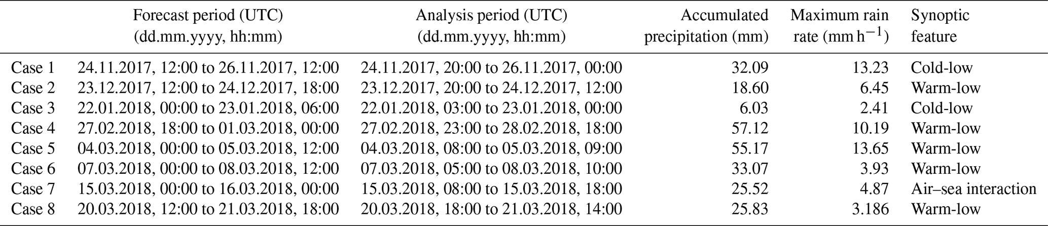
When the LPS located in the south of the polar jet passes over the southern part of Korea, widespread precipitation can occur over the southern and middle parts of the Korean Peninsula. Kim et al. (2021a) classified snowfall cases occurring under this synoptic situation as a warm-low type. One of the most significant characteristics of this pattern is the two different vertical layers (Tsai et al., 2018; Kim et al., 2018, 2021a, b): the deep system aloft (∼10 km height) is associated with LPS widespread precipitation with the westerly flow, whereas the other snowstorm below is associated with sea effect snow with the easterly or northeasterly flow (hereafter referred to as Kor'easterlies) (Park et al., 2020). Thus, the seeder–feeder effect is expected in this type of precipitation system. This vertical structure is maintained until the LPS-related widespread precipitation moves further east to the East Sea or Japan, followed by the shallow precipitation system with the Kor'easterlies-induced snow. Five warm-low events, cases 2, 4, 5, 6, and 8 in Table 1, were identified during the field campaign.
Snowfall cases associated with the air–sea interaction occur, accompanied by the Siberian high expansion toward the Kaema Plateau and/or East Sea. As the cold air from the north flows over the warm East Sea, a snow cloud is formed (Veals et al., 2019; Steenburgh and Nakai, 2020), and it is advected by the Kor'easterlies, resulting in frequent snowfall over the northeastern part of Korea. The depth of the snowfall system is generally shallower (less than ∼3 km height) than other types and is determined by the depth of the Kor'easterlies layer and the height of the thermal inversion layer above. The air–sea interaction is the most frequent synoptic scenario to produce heavy snowfall in the northeastern part of the Korean Peninsula (Cheong et al., 2006; Choi and Kim, 2010; Kim et al., 2021a). However, only one event, case 7 in Table 1, is identified during the ICE-POP 2018 field campaign. Our study selects cases 3, 6, and 7 as representative cases for the cold-low, warm-low, and air–sea interaction categories, respectively. A more detailed explanation of the characteristics of each category is provided in Kim et al. (2021a).
2.2 Observation data
The observed precipitation from the Korea Meteorological Administration Automatic Weather Station (AWS) during the analysis period for case 3, case 6, and case 7 is shown in Fig. 1. A heated tipping-bucket gauge was located on each station. The forecast and analysis period for each case is noted in Table 1 with the total accumulated rain (mm) and the maximum rain rates (mm h−1) during the analysis period. The spatial distribution of surface precipitation in case 3 is rather uniform (Fig. 1a), producing a maximum rain rate of 2.41 mm h−1. For case 6, surface precipitation is concentrated in the southeastern and coastal regions (Fig. 1b). The maximum rain rate along the coastal region is shown in case 7 (air–sea interaction). The observed maximum rain rate is 3.9 mm h−1 for case 6 and 4.87 mm h−1 for case 7. The greatest amount of precipitation is observed with case 4 (warm-low), and the least amount is with case 3 (cold-low) among the eight cases (Table 1).
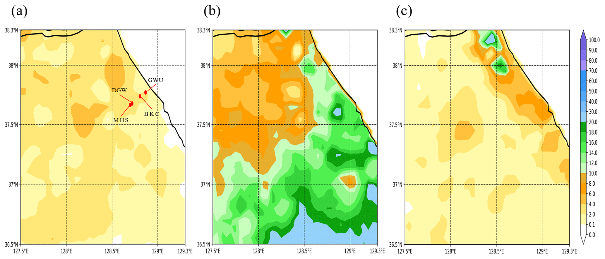
Figure 1Observed accumulated precipitation amount (mm) (a) for 21 h from 22 January, 03:00 UTC, to 23 January, 00:00 UTC (case 3), (b) for 29 h from 7 March, 05:00 UTC, to 8 March, 10:00 UTC (Case 6), and (c) for 10 h from 15 March, 08:00 UTC, to 15 March, 18:00 UTC (case 7), obtained from the AWS. The locations of one coastal site, Gangneung-Wonju National University (GWU), and three mountain sites, BoKwang 1-ri Community Center (BKC), DaeGwallyeong Regional Weather Office (DGW), and MayHills Supersite (MHS), are noted in (a).
Accurate measurement of precipitation by a heated tipping-bucket gauge is a challenge in windy environments. Strong winds lead to severe undercatch of snowfall amount, particularly for solid precipitation (Goodison et al., 1998; Thompson and Eidhammer, 2014; Kochendorfer et al., 2017; Smith et al., 2020). Other sources of measurement uncertainty include sublimation or evaporation on the heated gauge funnel (Rasmussen et al., 2012), orifice capping during heavy snowfall (Boudala et al., 2014), blowing snow (Geerts et al., 2015), and the representativeness of the observation, particularly in the mountainous region. Hence, it should be noted that the precipitation amount analyzed in this study may suffer from these sources of uncertainty, likely resulting in lower precipitation amounts. Despite these limitations, this study takes advantage of a dense network of heated tipping-bucket gauges, which is comprised of 129 stations within the studied area of about 160×200 km2. In addition, all gauges were equipped with a single shield that improves catch efficiency of snow in windy condition (Kochendorfer et al., 2017).
During the ICE-POP 2018 field campaign, remote sensing and in situ measurements for cloud properties were performed over the northeastern part of South Korea. The location of one coastal site, Gangneung-Wonju National University (GWU), and three mountain sites, DaeGwallyeong Regional Weather Office (DGW), MayHills Supersite (MHS), and BoKwang 1-ri Community Center (BKC), are noted in Fig. 1a. PARSIVEL disdrometers (Löffler-Mang and Joss, 2000; Tokay et al., 2014) at the GWU and DGW sites provide the frequency distributions of particle fall velocity as functions of diameter at the surface; thus, we can obtain the information about the surface precipitation type for each representative case, as shown in Fig. 2. At the coastal site, GWU, a mixture of snow- and liquid-type precipitation is measured for case 3. Case 6 is characterized by the liquid-type and graupel-like precipitation, and case 7 consists of the liquid-type precipitation. At the mountain site, DGW, a mixture of liquid-type precipitation with snow and graupel is observed in all cases, but a more intense signal of the liquid-type precipitation is seen in case 7.
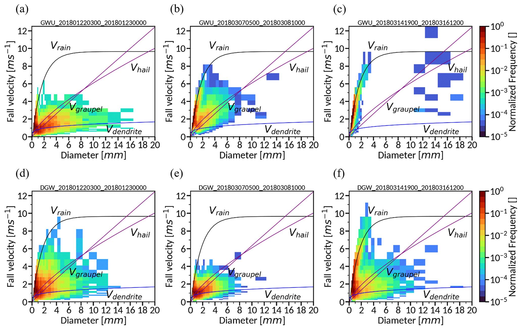
Figure 2Normalized frequency of the measured precipitation particle fall velocity as a function of diameters at the GWU (a–c) and DGW (d–f) sites. Panels (a) and (d) are for case 3, panels (b) and (e) are for case 6, and panels (c) and (f) are for case 7 during the analysis period. The solid lines represent the relationship between the fall velocity and diameter for rain (using the power law fit from the Gunn and Kinzer, 1949, data; Atlas et al., 1973), dendrite (derived from the observed data; Lee et al., 2015), graupel, and hail (derived from the observed data; Heymsfield et al., 2018) at sea level.
The MXPol radar measurement, located at the GWU site, provides the classified hydrometeor information along the direction between MHS and GWU. Figure 3 shows the area of hydrometeor types in which the hourly average fraction is larger than the threshold. The period is selected for the peak time of the domain-averaged rain for each case. The radar-classified hydrometeors are eight hydrometeor types based on the algorithm proposed by Besic et al. (2018): crystals (CR), aggregates (AG), light rain (LR), rain (RN), rimed ice particle (RP), wet snow (WS), ice hail and high-density graupel (IH), and melting hail (MH). The hydrometeors are not drawn over the region, where radar echoes are absent.
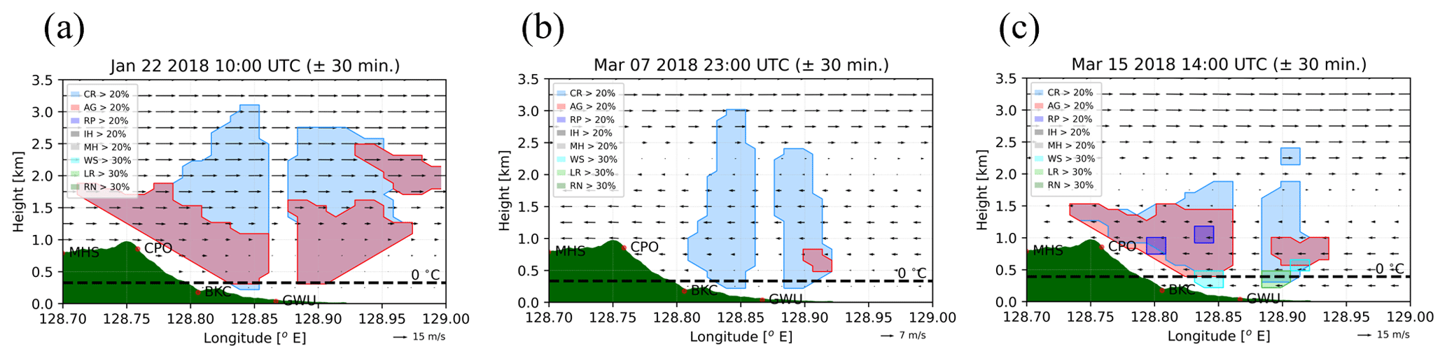
Figure 3Area of hydrometeor types in which the hourly average fraction of hydrometeors is larger than the threshold indicated. Hydrometeor types are derived from X-band Doppler dual-polarization radar (MXPol) along the direction between MHS and GWU sites at (a) 10:00 UTC on 22 January (case 3), (b) 23:00 UTC on 7 March (case 6), and (c) 14:00 UTC on 15 March (case 7). Eight hydrometeor categories, crystal (CR), aggregate (AG), rimed particle (RP), ice hail or graupel (IH), melting hail (MH), wet snow (WS), light rain (LR), and rain (RN) are identified. The green shading represents the terrain. The flows along the cross section, retrieved from multiple Doppler radars, are also drawn in each figure, and the vertical components of the arrows are upward air motion. The flows and classified hydrometeors are the versions that are averaged hourly.
CR is the primary hydrometeor type, and AG is between 1.5 and 3.0 km level in case 3 (Fig. 3a). For case 6, CR is also the major hydrometeor type over the entire observational region. A small portion of AG exists around the coastal GWU site at the 0.5 km level (Fig. 3b). Hydrometeors are mainly classified into CR, AG with a small portion of RP above the 0.5 km level, and WS and LR below the 0.5 km level from the observation for case 7 (Fig. 3c). The freezing level is drawn using the radiosonde observations at BKC site on 09:00 UTC 22 January, 00:00 UTC 8 March, and 15:00 UTC 15 March for each case. The retrieved wind fields (cross-barrier and vertical wind) from multiple surveillance Doppler radars (Liou and Chang, 2009; Tsai et al., 2018) are also represented in Fig. 3. The wind fields are the hourly averaged ones during the 1 h time window, centered at the maximum precipitation time. The westerly winds generally blow from mountains to the ocean and become stronger with higher altitude in case 3. Both case 6 and case 7 show the transition zone of wind fields, i.e., northeasterly below and southwesterly above. In general, the flow patterns follow the overall characteristics of winds well for three types of precipitation system (see Kim et al. 2021a).
2.3 Model design
The Advanced Research WRF model version 4.1.3 (Skamarock et al., 2019) is used for simulations. The WRF model is a non-hydrostatic compressible model with an Arakawa-C grid system and has several options for each physics parameterization. The model grids consist of three nested domains with a horizontal grid spacing of 9, 3, and 1 km (Fig. 4). The 65 vertical levels are configured with a 50 hPa model top. Table 2 shows the summary of the model configuration, including the number of model grids, the physics parameterization used, and initial or boundary conditions for model integration. The Kain–Fritsch (Kain and Fritsch, 1990; Kain, 2004) scheme is only applied to the outer domain of the 9 km resolution domain. The model forecast and analysis periods for each case are listed in Table 1. The model results are evaluated over the Yeongdong area of northeastern South Korea during the analysis period, represented as a dotted square in Fig. 4.
Figure 4Model domain consisting of the three nested domains with 9, 3, and 1 km resolutions centered on the Korean Peninsula. Shading indicates the terrain height (m) above the sea level, and latitudes and longitudes are denoted in the margins. The analysis domain is denoted with a dotted square inside of the innermost domain (d03).
Table 2Summary of the Weather Research and Forecasting (WRF) model configuration.
Four cloud microphysics parameterizations, namely WDM6 (Lim and Hong, 2010), WRF double-moment 7-class (WDM7) (Bae et al., 2019), Thompson (Thompson et al., 2008), and Morrison (Morrison et al., 2005), are used in our study. WDM6 and WDM7 schemes include the corrections for the numerical errors in ice microphysics parameterizations (Kim and Lim, 2021) and for cloud evaporation and melting processes (Lei et al., 2020). WDM6, Thompson, and Morrison parameterizations include five hydrometeor types: cloud water, rain, ice, snow, and graupel. WDM7 is developed on the basis of WDM6 by adding the prognostic variable of hail mixing ratio. WDM6 and WDM7 predict both number concentration and the mixing ratio for liquid particles but only the mixing ratio for solid-phase hydrometeors. The Thompson scheme predicts the number concentration and the mixing ratio for ice and rain but only the mixing ratio for other hydrometeors. In the Morrison scheme, the number concentration and the mixing ratio are predicted for all hydrometeors (except for cloud water, for which only the mixing ratio is predicted). There are aerosol-aware versions of the Thompson and Morrison schemes in the WRF model. However, we perform the model simulations using the Thompson and Morrison schemes, which do not include the aerosol activation processes; thus, two schemes do not predict the cloud water number concentration. Table 3 shows the prognostic variables for each microphysics scheme. The tested parameterizations are full or partially double-moment schemes, as shown in Table 3. For the microphysics budget analysis, the name of the source and sink terms in each microphysics scheme, which are differently designated, is matched, as shown in Table 4. For example, the cloud water condensation and evaporation process from all microphysics schemes is identically denoted as QCCON.
Table 3Four bulk-type cloud microphysics parameterizations and their prognostic variables. The existence of prognostic variables in each parameterization is denoted with “O” (existence) or “X” (nonexistence). NX and QX represent the number concentration and mixing ratio of a hydrometeor, X. The subscripted C, R, I, S, G, and H indicate cloud water, rain, cloud ice crystal, snow, graupel, and hail, respectively.
Table 4List of symbols for cloud microphysical processes in each microphysics scheme and their meaning. Differently named microphysical processes in each scheme are coordinated in our study using the names addressed in the “notation” row.
3.1 Cold-low cases
The simulation results for cold-low cases are presented in this section. Figure 5 shows the statistical skill scores of bias, root-mean-square error (RMSE), probability of detection (POD), and false alarm ratio (FAR) for the simulated precipitation using the WDM6, WDM7, Thompson, and Morrison schemes. White, black, yellow, and blue bars represent the results for the simulations with the WDM6, WDM7, Thompson, and Morrison schemes, respectively. The cold-low, warm-low, and air–sea interaction cases are shaded in blue, red, and green, respectively, on the x axis. We adopt the threshold value of 0.05 mm h−1 to judge the existence of precipitation when we calculate POD and FAR. The calculation method of POD and FAR follows the study of Rezacova et al. (2009). All microphysics parameterizations present a positive bias for against the surface precipitation. Thompson and Morrison simulations show better skill scores in bias, RMSE, and FAR compared to WDM6 and WDM7. The accumulated precipitation during the analysis period for case 3, the representative case of the cold-low type, is shown in Fig. 6a–d. All schemes simulate the precipitation as a type of snow over the northeastern part of the domain. WDM6 and WDM7 simulate more liquid rain at the surface precipitation than the Morrison and Thompson schemes. Simulated hydrometeor types at the surface are compared qualitatively with measurements using PARSIVEL disdrometers (Fig. 2). In case 3, the simulated hydrometeor types are snow and rain over the coast and mountains in all schemes (Fig. 6a–d). Although graupel-type precipitation is not predicted at the surface in all schemes, the overall features match well with the observations (Fig. 2a and d).
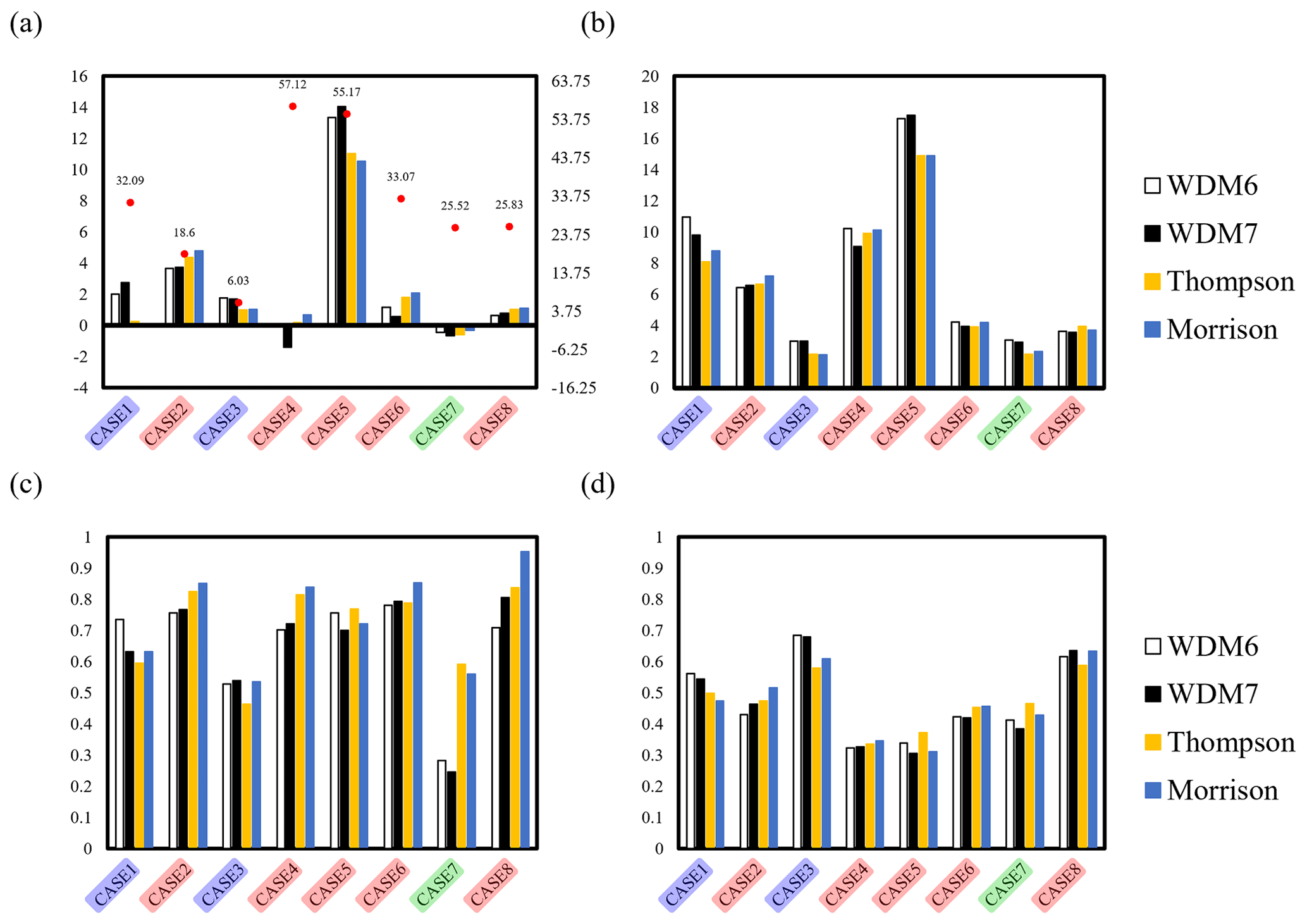
Figure 5Statistical skill scores of bias, root-mean-square error (RMSE), probability of detection (POD), and false alarm ratio (FAR) for the simulated precipitation with respect to the AWS observation. The units of bias and RMSE shown in (a) and (b) are given in millimeters. White, black, yellow, and blue bars represent the results for the simulations with the WDM6, WDM7, Thompson, and Morrison schemes. The cold-low, warm-low, and air–sea interaction cases are shaded in blue, red, and green on the x axis. The total cumulative precipitation (mm) for each case obtained from the AWS (Table 1) is also noted in (a) using red dots that relate to the scale on the right-hand y axis.
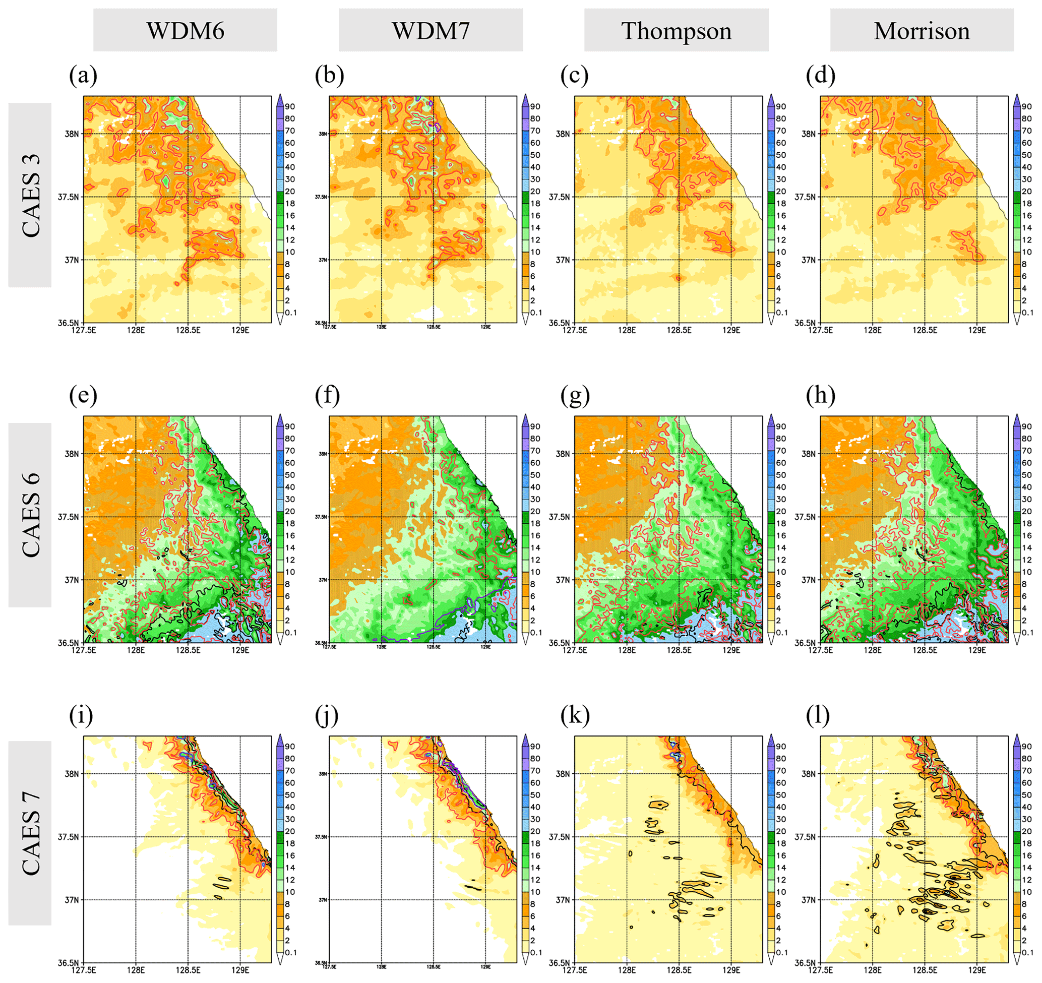
Figure 6Accumulated precipitation (mm) of the simulations using different cloud microphysics parameterizations during the analysis period. Panels (a)–(d) are for case 3, panels (b) and (e) are for case 6, and panels (c) and (f) are for case 7 during the analysis period. Panels (a)–(d) are for case 3, panels (e)–(h) are for case 6, and panels (j)–(l) are for case 7. The simulations in the first and second columns are conducted with the WDM6 and WDM7 schemes. The ones in the third and fourth columns are conducted with the Thompson and Morrison schemes. Black, red, blue, and purple contours represent the rain-, snow-, graupel-, and hail-type precipitation at the surface, respectively. The contour intervals for case 3, case 6, and case 7 are 3, 10, and 5 mm, respectively.
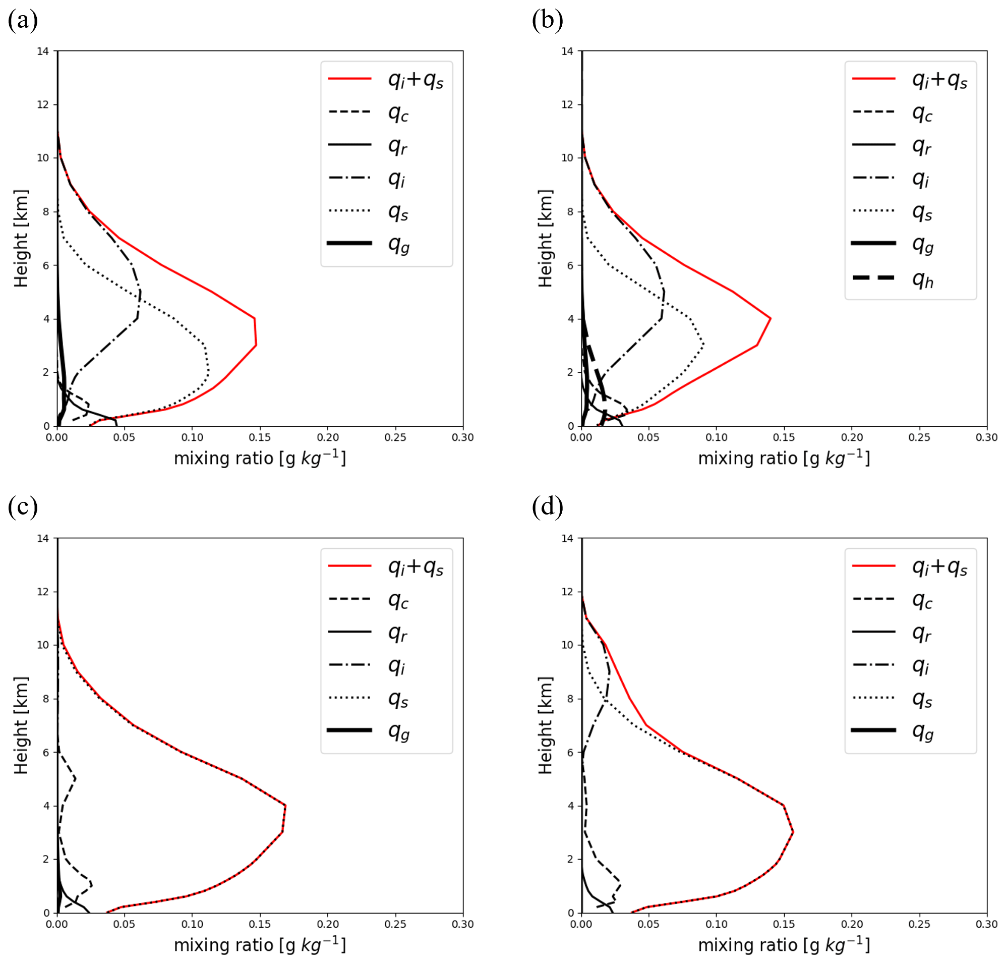
When the strongest domain-averaged precipitation intensity is observed, the simulated hydrometeors and wind are compared with the retrieved ones from radars along the cross section between GWU and MHS sites (Figs. 3a and 7a–d). For the comparison analysis, hydrometeor types of CR, AG, and IH from the retrievals can be regarded as cloud ice, snow, and hail in the model. The hydrometeor type of RP corresponds to graupel in the model. RN and MH can be considered rain in the model, and LR can be considered cloud water or rain. WS is not predicted by any of the microphysics schemes verified in our study. WDM6 and WDM7 simulate cloud ice over the entire region of the cross section above 2 km level. Furthermore, cloud ice is predicted, even near the mountain top, with a snow amount greater than 0.38 g kg−1 at around the 1.5 km level. However, both schemes miss the observed snow near the GWU site. The Thompson and Morrison schemes also simulate sufficient snow mass, showing its maximum near the mountain top. However, cloud ice is not simulated with both schemes. This is because Thompson and Morrison schemes efficiently transfer cloud ice to snow at the cut-off diameter of 200 and 250 µm; therefore, the schemes keep all cloud ice sizes relatively small. Over the mountain top where cloud ice is shown in WDM6 and WDM7, cloud water is simulated with the Thompson and Morrison schemes instead. More cloud ice with WDM6 and WDM7 can be also confirmed in the time-domain-averaged vertical profiles of hydrometeors (Fig. 8). As shown in Fig. 8a and b, the vertical distributions of hydrometeors from WDM6 and WDM7 are comparable in terms of the vertical extent and the maximum level of hydrometeors (except when it comes to hail). WDM7 has reduced snow compared to WDM6 and simulates as much hail as the reduction. The Thompson scheme rarely produces ice and shows the largest snow amount among the schemes used in the experiments. The Morrison scheme simulates cloud ice in layers between 3 and 6 km. Consistent with the hydrometeor distribution shown from the cross section, the Thompson and Morrison schemes produce more cloud water below 4 km level than WDM6 and WDM7 (Fig. 8c and d). In all experiments, the simulated winds blow from the inland to the ocean, consistently shown from the observation (Figs. 3a and 7a–d). Meanwhile, the simulated winds are weaker than the observation over the mountainous areas.

Figure 7Terrain and the simulated hydrometeor mixing ratio (g kg−1) along the cross section between GWU and MHS sites for (a–d) case 3, (e–h) case 6, and (i–l) case 7. From left to right, columns indicate the simulation results with the WDM6, WDM7, Thompson, and Morrison schemes, respectively. Shaded green and blue areas indicate the cloud water and ice mixing ratios, respectively. Red, blue, and black contours are for the snow, graupel, and hail mixing ratios. The contour levels are in 0.1 g kg−1 increments and the contour labels are in 0.2 g kg−1 increments starting from 0.1 g kg−1. The solid gray line represents the 0 ∘C line. The wind fields are overlaid at the same time.
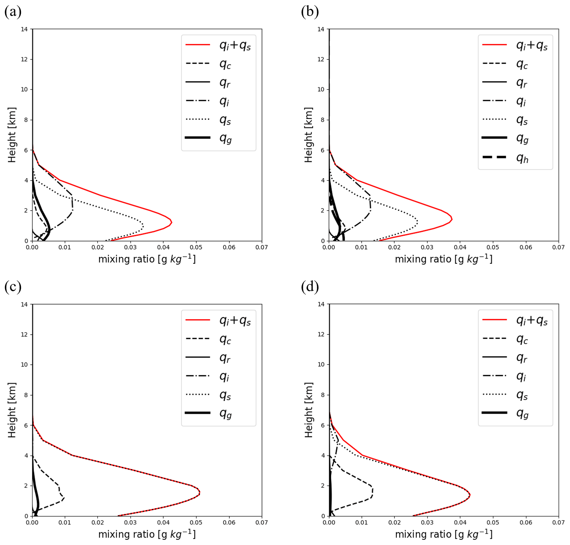
Figure 8Time-domain-averaged vertical hydrometeor mixing ratio profiles from the simulations using the (a) WDM6, (b) WDM7, (c) Thompson, and (d) Morrison schemes for case 3. The averaged time and domain are the same as that in Fig. 6. The sum of snow and cloud ice mixing ratios is drawn with a red line in all simulations.
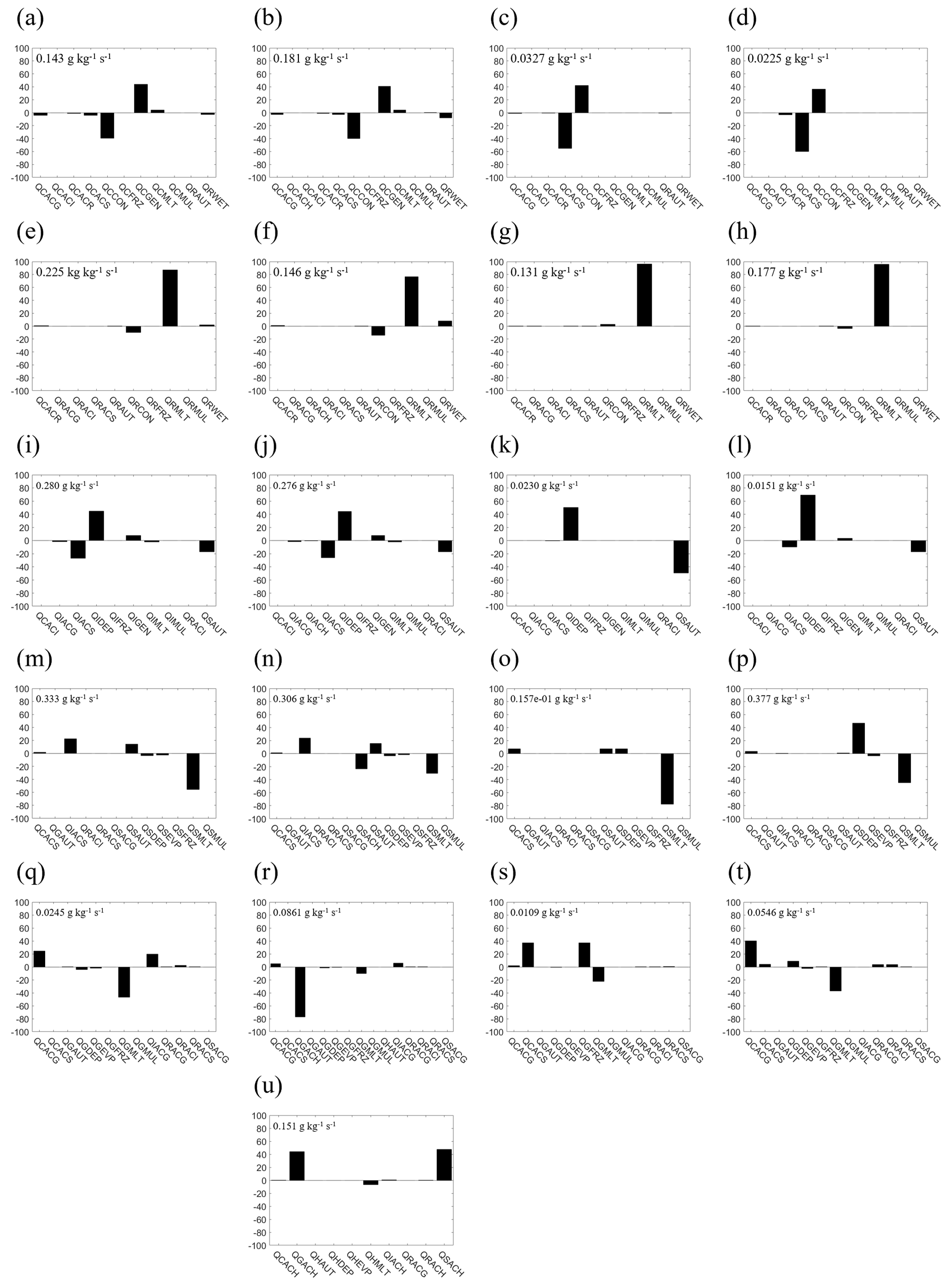
The relative contribution of microphysics processes in the production of each hydrometeor is compared among experiments in Fig. 9. The production rate of microphysical processes is averaged over the same analysis domain and duration, as considered in the precipitation and hydrometeor analysis shown in Figs. 5 and 6. The absolute values of every production rate to generate or dissipate a certain hydrometeor are summed, and each production rate is divided by the sum to generate a percentage. The positive rates in Fig. 9 indicate source processes for the hydrometeor, and the negative rates indicate sink processes. The contribution of sedimentation could be indirectly estimated from the hydrometeor mixing ratio and cloud microphysics budget amount. The cloud condensation nuclei (CCN) activation process (QCGEN) is the main source of cloud water in WDM6 and WDM7 (Fig. 9a and b). Meanwhile, cloud water in the Thompson and Morrison schemes is primarily generated by QCCON due to the absence of QCGEN (Fig. 9c and d). QCGEN only includes the condensation, but QCCON includes both condensation and evaporation. The negative sign of QCCON means that the magnitude of evaporation is greater than that of condensation. Note that we use the non-aerosol-aware version of the Thompson and Morrison schemes, which excludes aerosols and related microphysics processes. The collision and coalescence between cloud water and other hydrometeors (QCACR, QCACS, and QCACG) is the main sink for cloud water in all schemes. Besides these accretions, evaporation is another major sink of cloud water in WDM6 and WDM7. Most of the rain is produced by melting from solid-phase hydrometeors (QRMLT) (Fig. 9e–h) in all experiments and consumed by the evaporation process (QRCON), except for in the Thompson scheme.
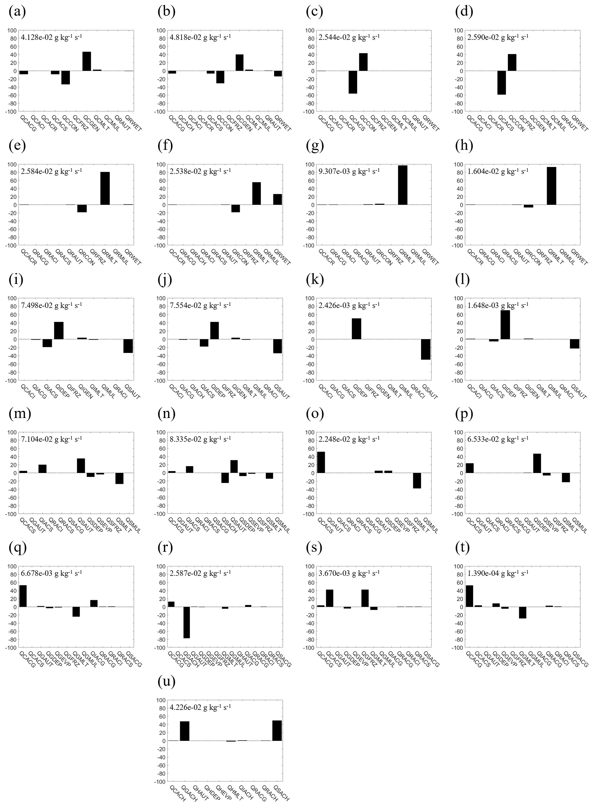
Figure 9Relative contribution of time-domain-averaged production tendency term during the analysis period. From left to right, columns indicate the simulation results with the WDM6, WDM7, Thompson, and Morrison schemes, respectively. Panels (a)–(d) are the terms for cloud water, panels (e)–(h) are the terms for rain, panels (i)–(l) are the terms for cloud ice, panels (m)–(p) are the terms for snow, panels (q)–(t) are the terms for graupel, and panel (u) is the terms for hail. The hail is only predicted in WDM7. In the upper-left corner of each panel, the sum of the absolute values of each production trend corresponding to 100 % is noted as the scaling number.
The deposition and sublimation of water vapor to cloud ice (QIDEP) is the primary source of cloud ice (Fig. 9i–l). Cloud ice decreases as it is converted into snow due to the auto-conversion process (QSAUT) and collision and coalescence process with snow (QIACS). The main processes to generate or deplete cloud ice are identical in all microphysics schemes. However, the absolute magnitude of QIDEP in WDM6 and WDM7, i.e., approximately 1.4 g kg−1, is greater than that in the Thompson and Morrison schemes (approximately 0.05 g kg−1), leading to more cloud ice generation. In WDM6 and WDM7, most of the snow is produced by QSAUT and QIACS, but in the Morrison scheme it is produced by QCACS and deposition from water vapor to snow (QSDEP) (Fig. 9m–o). QCACS is the primary source of snow in the Thompson scheme as well (Fig. 9p). Snow is depleted by a melting process (QSMLT) in all simulations. The accretion between snow and hail (QSACH) is also the primary sink of snow in WDM7. Meanwhile, graupel is mainly produced by the accretion process, QCACG, in WDM6(7) and the Morrison scheme. However, in the Thompson scheme, graupel is mainly produced by the freezing process (QGFRZ) and QCACS. WDM7, which additionally predicts hail, shows that the collision and coalescence between graupel and hail (QGACH) and QSACH are the major processes for hail generation. Meanwhile, Jang et al. (2021) showed that QGACH and QSACH can be eliminated by applying the mass-weighted terminal velocity for hail following the method by Dudhia et al. (2008); thus, the hail generation decreases considerably.
Except for the major sinks of graupel and snow, QGACH and QSACH, the responsible microphysical processes for generating hydrometeors in WDM6 and WDM7 are similar. The inclusion of aerosols in the microphysics processes causes the difference in major sources and sinks of cloud water, which can be seen from the comparison between WDM6(7) and the Thompson and Morrison schemes. In addition, more efficient cloud ice and inefficient cloud water production in WDM6(7), compared to the other schemes, cause the difference in the primary microphysics processes for snow production. Kim et al. (2021a) estimated possible microphysical processes from the measured particle size distribution and diameter for the cold-low case during ICE-POP 2018. Both aggregation and riming are analyzed as major processes to produce snow at the mountain site. Our analysis shows that aggregation is preferred in WDM6(7) and that riming is preferred in the Thompson and Morrison schemes at the top of the mountain (Fig. 7a–d). In addition, the enhanced melting of solid-phase particles in WDM6(7) compared to the Thompson scheme produces a lot of rain, resulting in a larger positive bias of simulated precipitation.
3.2 Warm-low cases
Simulated precipitation, hydrometeors, and microphysics budgets are compared for the warm-low cases in this section. The warm-low category includes five cases: cases 2, 4, 5, 6, and 8. Overall, all simulations in the warm-low category show better POD and FAR than those in the cold-low category (except for FAR in case 8). Consistent with the simulations for the cold-low category, all simulations in the warm-low category, except case 4 with WDM7 (Fig. 5), present a positive bias of surface precipitation. WDM6 overall shows the best bias scores. The Morrison scheme shows the best POD score but the worst bias, RMSE, and FAR, by producing abundant precipitation (except for in case 5). All simulations show the worst bias and RMSE scores for case 5 among the warm-low cases. The WDM6, Thompson, and Morrison schemes simulate the surface precipitation type as rain and snow (Fig. 6e, g, and h). However, WDM7 simulates a hail-type precipitation amount of more than 10 mm over the southeastern part of the analysis domain. Jang et al. (2021) noted that WDM7 generates too much hail regardless of the simulated convection. The area receiving the snow-type precipitation is confined to a narrow mountain region by WDM7 (Fig. 6f). The simulated hydrometeor types in all simulations are inconsistent with the observations, especially over the coastal region. The observation certainly shows graupel-like precipitation over the coastal region (Fig. 2b).
Figure 7e–h shows the simulated hydrometeors and wind fields for case 6, when the strongest domain-averaged precipitation intensity is observed. The simulated cloud ice appears just above the freezing level in WDM6 and WDM7. WDM7 simulates the freezing level lower than other schemes, which is not consistent with the observation (Figs. 7f and 3b). Meanwhile, the Thompson and Morrison schemes simulate a large amount of snow above the surface with an absence of cloud ice because these schemes only allow for the relatively small size of cloud ice. The WDM7, Thompson, and Morrison schemes simulate cloud water below the 0.5 km level over the coast. The vertical profiles of the time-domain-averaged hydrometeors present more snow and cloud water with the Thompson and Morrison schemes (Fig. 10c and d). Figure 10 also shows that WDM6 and WDM7 simulate more cloud ice between the 10 km level and the surface than other schemes. The Morrison scheme produces cloud ice between the 6 and 12 km levels, and the Thompson scheme simulates a low cloud ice amount. However, the sum of snow and cloud ice amount is greatest in the Thompson scheme. All cloud ice in the Thompson scheme is relatively small; therefore, its mixing ratio is nearly always an order of magnitude or more lower than other schemes. Kim et al. (2021a) mentioned that snowfall cases belonging to the warm-low category show the deepest systems and that precipitation is enhanced by the seeder–feeder mechanism with two different precipitation systems divided by wind fields, i.e., easterly below and westerly above. However, the transition layer of wind direction in all simulations is located at the higher latitude relative to the observed layer (compare Figs. 7e–h and 3b), which can cause a deficiency in simulating related microphysical mechanisms.
The relative contribution of microphysical processes to generate each hydrometeor among the schemes is compared in Fig. 11. QCGEN and QCCON are the primary sources for cloud water in the paired WDM6 and WDM7 and Thompson and Morrison schemes, respectively. The contribution of QRWET, responsible for generating rain, is reduced with WDM7 for the warm-low case compared to the cold-low case. QRMLT is still the primary source of rain in all simulations (Fig. 11e–h). The major sinks and sources of the liquid hydrometeors are identical between the warm-low and cold-low cases. The responsible microphysical processes for cloud ice formation and depletion are also identical to those for the cold-low case (Fig. 11i–l). The main source of cloud ice is QIDEP in all simulations. The magnitude of QIDEP in WDM6 and WDM7 is 5.5 g kg−1, which is approximately 10 times larger than that of the Thompson and Morrison schemes, leading to an abundant production of cloud ice greater than 0.06 g kg−1 (Fig. 10a and b).
The melting processes (QSMLT, QGMLT, and QHMLT) are the primary sinks of solid-phase precipitating particles such as snow, graupel, and hail in all simulations. The relative contribution of melting for the warm-low case, case 6, is greater than that for the cold-low case, case 3, due to the warm environment and the extended vertical range of solid-phase hydrometeors (Fig. 10m–u). All simulations show that the magnitude of QRMLT in case 6 is approximately 10 times larger than that in case 3. The melting process can largely affect rain production, resulting in surface precipitation in the warm-low case. The contribution of QCACS to snow generation is significantly decreased in the Thompson and Morrison schemes in the warm-low case compared to the cold-low case. This is because of the reduced cloud water in case 6 with the Thompson and Morrison schemes compared to case 3. In both schemes, cloud water generation is suppressed in the warm-low case. Even though both QSAUT and QIACS are still the major sources of snow production in WDM6 and WDM7, the contribution of QSAUT decreases, and the contribution of QIACS increases in WDM6 and WDM7 in the warm-low case compared to the cold-low case. There is no distinct discrepancy for the key microphysical processes of graupel (and hail) formation and depletion between the warm-low and cold-low cases.
3.3 Air–sea interaction cases
Statistical skill scores for the simulated precipitation are presented in Fig. 5 for the air–sea interaction case. Only one case, case 7, is classified as an air–sea interaction category during the ICE-POP 2018 field campaign, presenting a negative bias. Overall, Morrison shows the best skill scores for the simulated precipitation. The POD from simulations with WDM6 and WDM7 show the worst scores due to the missing precipitation events over the southwestern part of the analysis domain (Figs. 1c and 6i, j). The precipitation system, which is initiated by air-mass transformation over the East Sea, propagates to inland areas by the easterly winds. Therefore, the precipitation area is restricted in the eastern area of the Korean Peninsula, and intense precipitation is presented along the coast in both the observation and simulations (Fig. 6i–l). WDM6 and WDM7 simulate solid-phase precipitation amounts more than 14 mm. In addition, WDM7 produces hail-type precipitation over the coast. The precipitation type simulated with WDM6 and WDM7 does not match with the observed types, especially over the coast (Figs. 2 and 6i–l). Observation shows pure liquid-type precipitation, but both simulations produce excess solid-phase precipitation.
The simulated hydrometeor distribution and wind fields over the cross section are compared to the observations (Figs. 3 and 7i–l). When the strongest domain-averaged precipitation intensity is observed, all simulations produce a significant amount of cloud water below the 3 km level. A large amount of cloud water in the simulations can be also confirmed in the time-domain-averaged vertical profiles of hydrometeors (Fig. 12). In all simulations, simulated hydrometeors are confined to below the 4 km level. WDM6 and WDM7 produce the largest amount of cloud water and cloud ice and snow. The experiment with the Morrison scheme simulates more rain than other simulations (Fig. 12d). WDM6 and WDM7 simulate cloud ice with some snow and graupel below the 2 km level, which is consistent with the observation in which CR, AG, and RP are seen (Figs. 3 and 7i, j). However, the region with the graupel (RP in the observation) is shifted to the coastal region in WDM6 and WDM7, generating excess solid-phase precipitation over the coast. Consistent with other cases, the Thompson and Morrison schemes do not simulate cloud ice at the maximum precipitation time. The Morrison scheme simulates snow between the surface and 2 km level, representing its maximum at the coastal GWU site (Fig. 7l). All experiments show the westerly wind over the ocean and coastal area, indicating that they fail to simulate the Kor'easterlies, which is the most important dynamical characteristic of the air–sea interaction category.
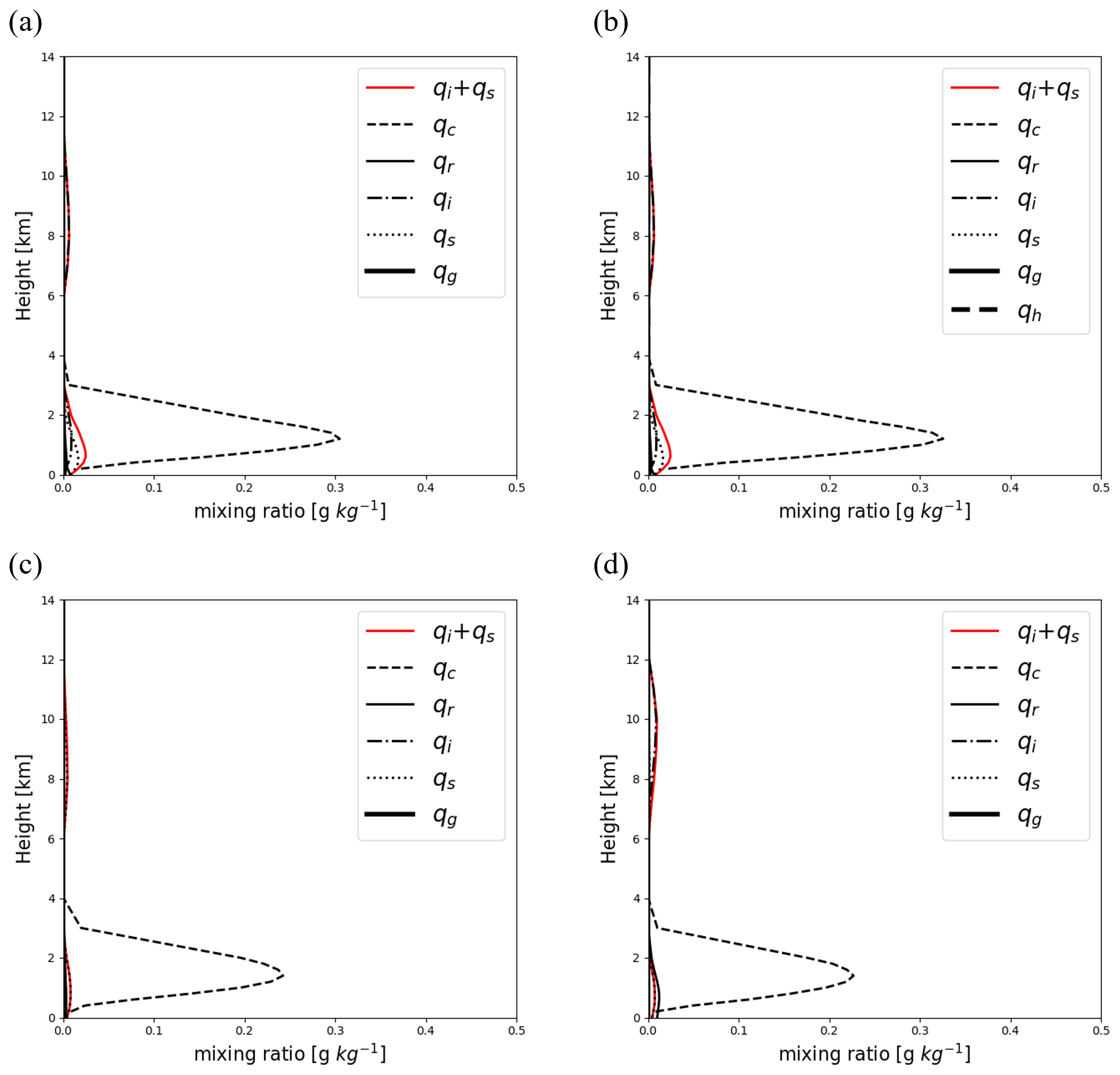
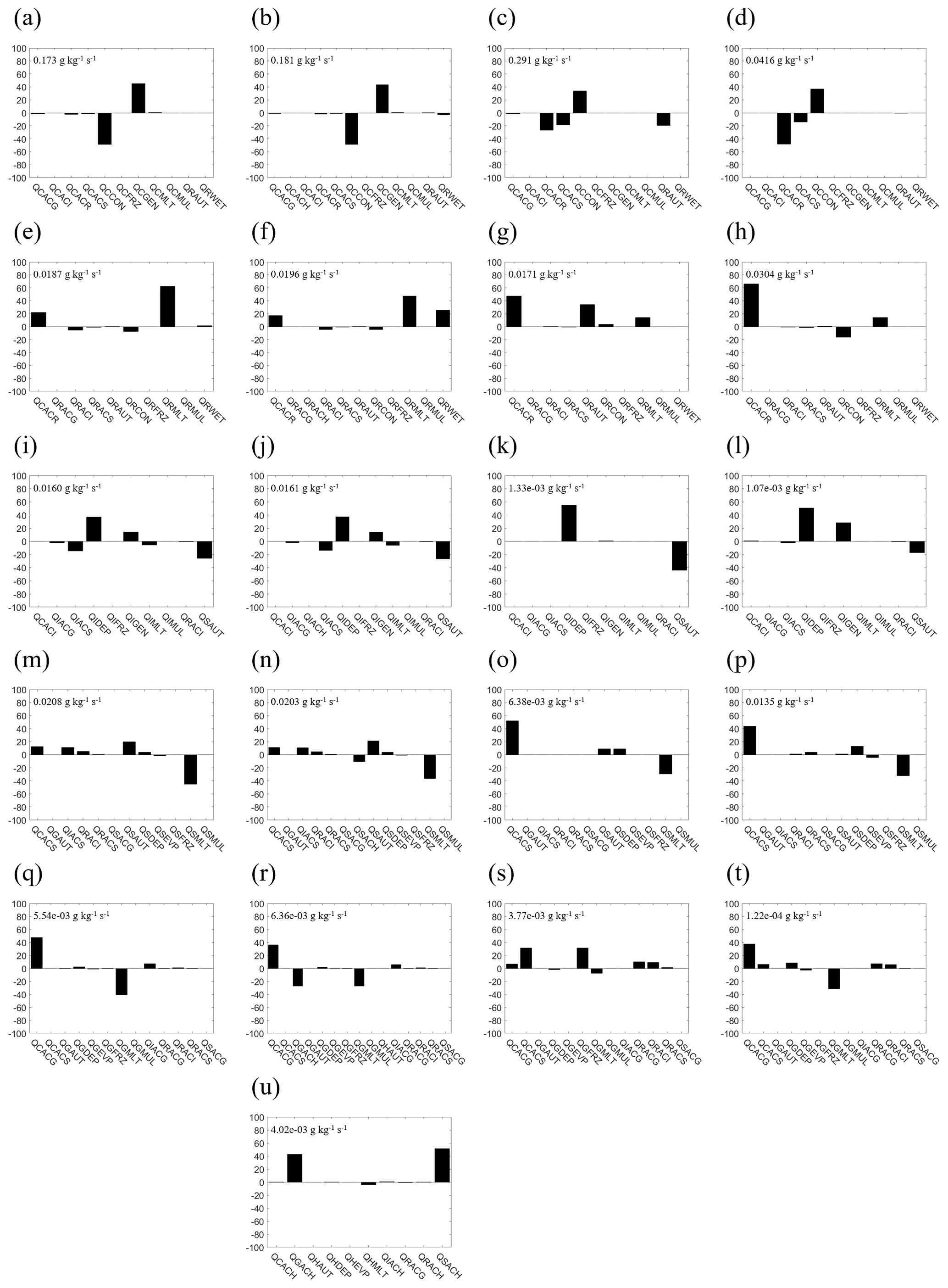
Figure 13 shows the relative contribution of microphysical processes for case 7. Unlike the cold-low and warm-low cases, cloud water is mainly depleted by QCACR in the Thompson and Morrison scheme due to decreased snow production in the air–sea interaction case. The primary source and sinks for cloud water are not changed in WDM6 and WDM7. In all simulations, the relative contribution of QRMLT to the generation of rain decreases, and the contribution of cloud water-to-rain processes such as QCACR, QRAUT, and QRWET increases. In particular, QCACR and QRAUT are the main sources of rain in the Thompson scheme, and QCACR is the main source of rain in the Morrison scheme. For cloud ice, QIDEP and the generation of ice by nucleation and CCN activation (QIGEN) are analyzed as the major sources in all simulations. The contribution of QIGEN in cloud ice production increases compared to cold-low and warm-low cases. In the WDM6 and WDM7 schemes, the magnitude of QIDEP is 0.27 g kg−1, which is about 10 times larger than that in the Thompson and Morrison schemes. In all simulations, the relative contribution of QCACS to the formation of snow increases due to increased cloud water generation, and those of QIACS and QSAUT decrease with the decreased cloud ice generation. However, QIACS and QSAUT in both WDM6 and WDM7 are still major sources of snow. In the Morrison scheme, the contribution of QSDEP to snow formation is significantly reduced in the air–sea interaction case unlike the cold-low and warm-low cases. Several microphysics processes are involved in graupel formation with the Thompson scheme for the air–sea interaction case, but the formed graupel amount is not identified in the surface precipitation.
This study evaluates the performance of four microphysics parameterizations, the WDM6, WDM7, Thompson, and Morrison schemes, which have been widely used as cloud microphysics options in the WRF model, when simulating snowfall events during the ICE-POP 2018 field campaign. Eight snowfall events are selected and classified into three categories (cold-low, warm-low, and air–sea interaction) depending on their synoptic characteristics. The evaluation is conducted focusing on the simulated hydrometeors, microphysics budgets, wind fields, and precipitation using the measurement data from MXPol radar, multiple surveillance Doppler radars, PARSIVEL disdrometers, and AWS. Most simulations show a deficiency of a positive bias in the simulated precipitation for the cold-low and warm-low cases. The simulations for the air–sea interaction case present a negative bias and show the best bias score. Overall, the modeled precipitation for the warm-low cases shows a better POD score than that for the cold-low and air–sea interaction cases.
The simulated hydrometeor types at the surface for the cold-low case are snow and rain over both coastal and mountainous regions, regardless of the microphysics schemes, which is consistent with the observed features. Both WDM6 and WDM7 simulate an abundant amount of cloud ice and snow, especially over the mountain top and its downslope region when the strongest precipitation intensity is observed. The retrievals from the radar also classify cloud ice and snow as primary hydrometeor types over the downslope region of the mountain top. The Thompson and Morrison schemes simulate sufficient snow amount; however, neither of these schemes produce cloud ice over the downslope region because they keep all cloud ice relatively small compared to WDM6 and WDM7. In all experiments, the simulated winds blow from the inland to the ocean, as observed in the Doppler radar-retrieved one. Most of the rain mixing ratio is produced by melting in all experiments. The primary processes that generate or deplete cloud ice are identical in all microphysical schemes, which are the deposition for the formation and conversion to snow or collision and coalescence for depletion. Snow is mainly generated by aggregation in WDM6 and WDM7, but the accretion between snow and cloud water and deposition is mainly generated in the Thompson and Morrison schemes.
For the warm-low case, all experiments mainly produce rain and snow-type surface precipitation over the coastal and mountainous areas. WDM7 predicts hail-type precipitation amount more than 10 mm, which is not observed. The simulated hydrometeor types in all simulations are inconsistent with the observations, which shows graupel-like precipitation especially over the coastal region. WDM6 and WDM7 simulate the cloud ice amount between 0.01 and 0.1 g kg−1 near the coast site when the maximum precipitation is observed. Meanwhile, the Thompson and Morrison schemes simulate more snow over the corresponding region compared toWDM6 and WDM7. Although the simulated precipitation skill scores for the warm-low category are the best among all simulated categories, all simulations have a problem, i.e., the lower wind transition layer compared to the observed transition layer. Through the microphysics budget analysis, it is found that the major sources and sinks of hydrometeors are identical between the cold-low and warm-low cases. Meanwhile, the magnitude of melting is significantly enhanced in warm-low cases compared to cold-low cases due to the warmer environment and more available solid-phase hydrometeors. The relative contribution of collision and coalescence between cloud water and snow to produce snow is decreased compared to cold-low cases in the simulations with the Thompson and Morrison schemes, which is due to the reduced cloud water. For the air–sea interaction case, WDM6 and WDM7 simulate surface precipitation as a solid-phase type along the coast, which is inconsistent with the observation. This is because WDM6 and WDM7 produce excessive cloud ice amount with graupel and snow over the coast. In addition, none of the experiments simulate the low-level Kor'easterlies. Unlike the cold-low and warm-low cases, simulations for the air–sea interaction case produce abundant cloud water amount greater than 0.2 g kg−1 abundant cloud water. Therefore, rain is generated in large amounts by cloud collision and coalescence of cloud water and not primarily from melting.
More cloud ice generation with WDM6 and WDM7 and more cloud water generation with the Thompson and Morrison schemes are distinct in all cases. Therefore, the major microphysical processes to generate snow are significantly related with cloud ice in WDM6 and WDM7 and with cloud water in the Thompson and Morrison schemes. The Thompson (or Morrison) scheme transfers the cloud ice to snow at the diameter of 200 or 250 µm; therefore, more snow exists relative to the WDM6 and WDM7 schemes in which the maximum allowable diameter of cloud ice is 500 µm. Melting is the major process to produce rain in warm-low and cold-low cases. Therefore, the positive precipitation bias revealed from the warm-low and cold-low cases can be mitigated by modulating the melting efficiency in all schemes. Microphysics budget analysis shows that the inclusion of the prognostic variable of CCN number concentration changes the major source of cloud water production. CCN activation is the major process to produce cloud water with WDM6 and WDM7, with the CCN number concentration serving as a prognostic variable, but the condensation is the major process for cloud water generation with the Thompson and Morrison schemes. Our study also shows that the additional prognostic variable of hail has no advantage in simulating precipitation and hydrometeor profiles and produces excessive hail at the surface for the snowfall event that occurs over the complex terrain region in the eastern part of the Korean Peninsula. Even though several studies simulated snow storm cases under a horizontal resolution of 1 or 1.33 km (Alcott and Steenburgh, 2013; Molthan et al., 2016; Vignon et al., 2019; Veals et al., 2020), the 1 km horizontal resolution used in our study could be coarse for some generating cells during the winter season.
The source code of the WRF model version 4.1.3 is available at https://github.com/wrf-model/WRF/releases (Skamarock et al., 2019). The ERA-Interim reanalysis data from the European Centre for Medium-Range Weather Forecasts (ECMWF) for initial and boundary conditions are available at https://apps.ecmwf.int/datasets/data/interim-full-daily/levtype=pl/ (Dee et al., 2011a) and https://apps.ecmwf.int/datasets/data/interim-full-daily/levtype=sfc/ (Dee et al., 2011b). The model codes and scripts that cover every data- and figure-processing action for all the results reported in this paper are available at https://doi.org/10.5281/zenodo.5876054 (Ko et al., 2022). The observational data, such as the PARSIVEL and MXPol radar, are available via https://doi.org/10.5067/GPMGV/ICEPOP/APU/DATA101 (Petersen and Tokay, 2019) and https://doi.org/10.1594/PANGAEA.918315 (Gehring et al., 2020a). Model outputs are available upon request (Jeong-Su Ko via jsko@knu.ac.kr).
JSK designed and performed the model simulations and analysis under the supervision of KSSL. KSSL and JSK wrote the manuscript with substantial contributions from all co-authors. KK processed the observational data. KSSL, GL, AB, and GT contributed to the scientific discussions and gave constructive advice. KK and AB carried out the PARSIVEL and radar measurements.
The contact author has declared that neither they nor their co-authors have any competing interests.
Publisher's note: Copernicus Publications remains neutral with regard to jurisdictional claims in published maps and institutional affiliations.
The authors are greatly appreciative to the participants of the World Weather Research Program Research Development Project and Forecast Demonstration Project, International Collaborative Experiments for Pyeongchang 2018 Olympic and Paralympic winter games (ICE-POP 2018), hosted by the Korea Meteorological Administration. The authors would also like to thank Josué Gehring, Nikola Besic, and Alfonso Ferrone for their contributions to the operation and maintenance of the MXPol radar and for providing the hydrometeor classification product (https://doi.org/10.1594/PANGAEA.918315, Besic et al., 2018; Gehring et al., 2020a; Gehring et al., 2021) and Walter A Petersen and Ali Tokay for their contributions to the PARSIVEL data product (Petersen and Tokay, 2019).
This research has been supported by the South Korean Ministry of Science and ICT (MSIT) and the National Research Foundation of Korea (NRF) (grant no. 2021R1A4A1032646).
This paper was edited by Jinkyu Hong and reviewed by two anonymous referees.
Alcott, T. I. and Steenburgh, W. J.: Orographic influences on a Great Salt Lake–effect snowstorm, Mon. Weather Rev., 141, 2432–2450, https://doi.org/10.1175/MWR-D-12-00328.1, 2013.
Atlas, D., Srivastava, R. C., and Sekhon, R. S.: Doppler radar characteristics of precipitation at vertical incidence, Rev. Geophys., 11, 1–35, https://doi.org/10.1029/RG011i001p00001, 1973.
Bae, S. Y., Hong, S. Y., and Tao, W. K.: Development of a single-moment cloud microphysics scheme with prognostic hail for the Weather Research and Forecasting (WRF) model, Asia-Pacific J. Atmos. Sci., 55, 233–245, https://doi.org/10.1007/s13143-018-0066-3, 2019.
Bao, J.-W., Michelson, S. A., and Grell, E. D.: Microphysical process comparison of three microphysics parameterization schemes in the WRF model for an idealized squall-line case study, Mon. Weather Rev., 147, 3093–3120, https://doi.org/10.1175/MWR-D-18-0249.1, 2019.
Besic, N., Gehring, J., Praz, C., Figueras i Ventura, J., Grazioli, J., Gabella, M., Germann, U., and Berne, A.: Unraveling hydrometeor mixtures in polarimetric radar measurements, Atmos. Meas. Tech., 11, 4847–4866, https://doi.org/10.5194/amt-11-4847-2018, 2018.
Boudala, F. S., Isaac, G. A., Rasmussen, R., Cober, S. G., and Scott, B.: Comparison of snowfall measurements in complex terrain made during the 2010 Winter Olympics in Vancouver, Pure Appl. Geophys., 171, 113–127, https://doi.org/10.1007/s00024-012-0610-5, 2014.
Chen, F. and Dudhia, J.: Coupling an advanced land surface–hydrology model with the Penn State–NCAR MM5 modeling system. Part I: Model implementation and sensitivity, Mon. Weather Rev., 129, 569–585, https://doi.org/10.1175/1520-0493(2001)129<0569:CAALSH>2.0.CO;2, 2001.
Cheong, S.-H., Byun, K.-Y., and Lee, T.-Y.: Classification of snowfalls over the Korean Peninsula based on developing mechanism, Atmosphere, 16, 33–48, 2006.
Choi, G. and Kim, J.: Surface synoptic climatic patterns for heavy snowfall events, J. Korean Geogr. Soc., 45, 319–341, 2010.
Conrick, R. and Mass, C. F.: Evaluating simulated microphysics during OLYMPEX using GPM satellite observations, J. Atmos. Sci. 76, 1093–1105, https://doi.org/10.1175/JAS-D-18-0271.1, 2019.
Das, S. K., Hazra, A., Deshpande, S. M., Krishna, U. M., and Kolte, Y. K.: Investigation of cloud microphysical features during the passage of a tropical mesoscale convective system: Numerical simulations and X-band radar observations, Pure Appl. Geophys., 178, 185–204, https://doi.org/10.1007/s00024-020-02622-w, 2021.
Dee, D. P., Uppala, S. M., Simmons, A. J., Berrisford, P., Poli, P., Kobayashi, S., Andrae, U., Balmaseda, M. A., Balsamo, G., Bauer, P., Bechtold, P., Beljaars, A. C. M., van de Berg, L., Bidlot, J., Bormann, N., Delsol, C., Dragani, R., Fuentes, M., Geer, A. J., Haimberger, L., Healy, S. B., Hólm, E. V., Isaken, L., Kållberg, P., Köhlerm, M., Matricardi, M., McNally, A. P., Monge-Sanz, B. M., Morcrette, J.-J., Park, B.-K., Peubey, C., de Rosnay, P., Tavolato, C., Thépaut, J.-N., and Vitart, F.: The ERA-Interim reanalysis: configuration and performance of the data assimilation system, Q. J. R. Meteorol. Soc., 137, 553–597, https://doi.org/10.1002/qj.828, 2011a (data available at: https://apps.ecmwf.int/datasets/data/interim-full-daily/levtype=pl/, last access: October 2019).
Dee, D. P., Uppala, S. M., Simmons, A. J., Berrisford, P., Poli, P., Kobayashi, S., Andrae, U., Balmaseda, M. A., Balsamo, G., Bauer, P., Bechtold, P., Beljaars, A. C. M., van de Berg, L., Bidlot, J., Bormann, N., Delsol, C., Dragani, R., Fuentes, M., Geer, A. J., Haimberger, L., Healy, S. B., Hólm, E. V., Isaken, L., Kållberg, P., Köhlerm, M., Matricardi, M., McNally, A. P., Monge-Sanz, B. M., Morcrette, J.-J., Park, B.-K., Peubey, C., de Rosnay, P., Tavolato, C., Thépaut, J.-N., and Vitart, F.: The ERA-Interim reanalysis: configuration and performance of the data assimilation system, Q. J. R. Meteorol. Soc., 137, 553–597, https://doi.org/10.1002/qj.828, 2011b (data available at: https://apps.ecmwf.int/datasets/data/interim-full-daily/levtype=sfc/, last access: October 2019).
Dudhia, J., Hong, S. Y., and Lim, K. S.: A new method for representing mixed-phase particle fall speeds in bulk microphysics parameterization, J. Meteorol. Soc. Jpn., 86, 33–44, https://doi.org/10.2151/jmsj.86A.33, 2008.
Fan, J., Han, B., Varble, A., Morrison, H., North, K., Kollias, P,, Chen, B., Dong, X., Giangrande S. E., Khain, A., Lin, Y., Mansell, E., Millbrandt, J. A., Stenz, R., Thompson, G., and Wang, Y. : Cloud-resolving model intercomparison of an MC3E squall line case: Part 1-Convective updrafts, J. Geophys. Res. Atmos., 122, 9351–9378, https://doi.org/10.1002/2017JD026622, 2017.
Geerts, B., Yang, Y., Rasmussen, R., Haimov, S., and Pokharel, B.: Snow growth and transport patterns in orographic storms as estimated from airborne vertical-plane dual-doppler radar data, Mon. Weather Rev., 143, 644–665, https://doi.org/10.1175/MWR-D-14-00199.1, 2015.
Gehring, J., Ferrone, A., Billault-Roux, A. C., Besic, N., and Berne, A.: Radar and ground-level measurements of precipitation during the ICE-POP 2018 campaign in South-Korea, PANGAEA [data set], https://doi.org/10.1594/PANGAEA.918315, 2020a.
Gehring, J., Oertel, A., Vignon, É., Jullien, N., Besic, N., and Berne, A.: Microphysics and dynamics of snowfall associated with a warm conveyor belt over Korea, Atmos. Chem. Phys., 20, 7373–7392, https://doi.org/10.5194/acp-20-7373-2020, 2020b.
Gehring, J., Ferrone, A., Billault-Roux, A.-C., Besic, N., Ahn, K. D., Lee, G., and Berne, A.: Radar and ground-level measurements of precipitation collected by the École Polytechnique Fédérale de Lausanne during the International Collaborative Experiments for PyeongChang 2018 Olympic and Paralympic winter games, Earth Syst. Sci. Data, 13, 417–433, https://doi.org/10.5194/essd-13-417-2021, 2021.
Goodison, B. E., Louie P. Y. T., and Yang, D.: WMO solid precipitation intercomparison, Tech. Rep. WMO/TD-872, World Meteorological Organization, Geneva, 1998.
Gunn, R. and Kinzer, G. D.: The terminal velocity of fall for water droplets in stagnant air, J. Atmos. Sci., 6, 243–248, https://doi.org/10.1175/1520-0469(1949)006<0243:TTVOFF>2.0.CO;2, 1949.
Han, M., Braun, S. A., Matsui, T., and Williams, C. R.: Evaluation of cloud microphysics schemes in simulations of a winter storm using radar and radiometer measurements, J. Geophys. Res.-Atmos., 118, 1401–1419, https://doi.org/10.1002/jgrd.50115, 2013.
Heymsfield, A., Szakáll, M., Jost, A., Giammanco, I., and Wright, R.: A comprehensive observational study of graupel and hail terminal velocity, mass flux, and kinetic energy, J. Atmos. Sci., 75, 3861–3885, https://doi.org/10.1175/JAS-D-18-0035.1, 2018.
Hong, S. Y., Noh, Y., and Dudhia, J.: A new vertical diffusion package with an explicit treatment of entrainment processes, Mon. Weather Rev., 134, 2318–2341, https://doi.org/10.1175/MWR3199.1, 2006.
Huang, Y., Wang, Y., Xue, L., Wei, X., Zhang, L., and Li, H.: Comparison of three microphysics parameterization schemes in the WRF model for an extreme rainfall event in the coastal metropolitan City of Guangzhou, China, Atmos. Res., 240, 104939, https://doi.org/10.1016/j.atmosres.2020.104939, 2020.
Iacono, M. J., Delamere, J. S., Mlawer, E. J., Shephard, M. W., Clough, S. A., and Collins, W. D.: Radiative forcing by long-lived greenhouse gases: Calculations with the AER radiative transfer models, J. Geophys. Res., 113, D13103, https:/doi.org/10.1029/2008JD009944, 2008.
Jang, S., Lim, K. S. S., Ko, J., Kim, K., Lee, G., Cho, S. J., Ahn, K. D., and Lee, Y. H.: Revision of WDM7 microphysics scheme and evaluation for precipitating convection over the Korean peninsula, Remote Sens., 13, 3860, https://doi.org/10.3390/rs13193860, 2021.
Jeoung, H., Liu, G., Kim, K., Lee, G., and Seo, E.-K.: Microphysical properties of three types of snow clouds: implication for satellite snowfall retrievals, Atmos. Chem. Phys., 20, 14491–14507, https://doi.org/10.5194/acp-20-14491-2020, 2020.
Jiménez, P. A., Dudhia, J., González-Rouco, J. F., Navarro, J., Montávez, J. P., and García-Bustamante, E.: A revised scheme for the WRF surface layer formulation, Mon. Weather Rev., 140, 898–918, https:/doi.org/10.1175/MWR-D-11-00056.1, 2012.
Kain, J. S.: The Kain–Fritsch convective parameterization: an update, J. Appl. Meteorol. Climatol., 43, 170–181, https://doi.org/10.1175/1520-0450(2004)043<0170:TKCPAU>2.0.CO;2, 2004.
Kain, J. S. and Fritsch, J. M.: A one-dimensional entraining/detraining plume model and its application in convective parameterization, J. Atmos. Sci., 47, 2784–2802, 1990.
Kim, K., Bang, W., Chang, E.-C., Tapiador, F. J., Tsai, C.-L., Jung, E., and Lee, G.: Impact of wind pattern and complex topography on snow microphysics during International Collaborative Experiment for PyeongChang 2018 Olympic and Paralympic winter games (ICE-POP 2018), Atmos. Chem. Phys., 21, 11955–11978, https://doi.org/10.5194/acp-21-11955-2021, 2021a.
Kim, K. B. and Lim, K.-S. S.: The numerical error in WDM6 and its impacts on the simulated precipitating convections, AOGS 18th Annual Meeting, Online, 2–6 August 2021, AS23-A005, https://meetmatt-svr.net/Timetable/SlotScheduleAll?cfId=3&dayId=16&slotId=17&sId=1 (last access: June 2022), 2021.
Kim, Y. J., Kim, B. G., Shim, J. K., and Choi, B. C.: Observation and numerical simulation of cold clouds and snow particles in the Yeongdong region, Asia Pac. J. Atmos. Sci., 54, 499–510, https://doi.org/10.1007/s13143-018-0055-6, 2018.
Kim, Y. J., In, S. R., Kim, H. M., Lee, J. H., Kim, K. R., Kim, S., and Kim, B. G.: Sensitivity of snowfall characteristics to meteorological conditions in the Yeongdong region of Korea, Adv. Atoms. Sci., 38, 413–429, https://doi.org/10.1007/s00376-020-0157-9, 2021b.
Ko, J.-S., Lim, K.-S. S., Kim, K., Lee, G., Thompson, G., an Berne, A.: Code for GMD publication – Simulated microphysical properties of winter storms from bulk-type microphysics schemes and their evaluation in WRF (v4.1.3) model during ICE-POP 2018, Zenodo [data set], https://doi.org/10.5281/zenodo.5876054, 2022.
Kochendorfer, J., Nitu, R., Wolff, M., Mekis, E., Rasmussen, R., Baker, B., Earle, M. E., Reverdin, A., Wong, K., Smith, C. D., Yang, D., Roulet, Y.-A., Buisan, S., Laine, T., Lee, G., Aceituno, J. L. C., Alastrué, J., Isaksen, K., Meyers, T., Brækkan, R., Landolt, S., Jachcik, A., and Poikonen, A.: Analysis of single-Alter-shielded and unshielded measurements of mixed and solid precipitation from WMO-SPICE, Hydrol. Earth Syst. Sci., 21, 3525–3542, https://doi.org/10.5194/hess-21-3525-2017, 2017.
Lee, J. E., Jung, S. H., Park, H. M., Kwon, S., Lin, P. L., and Lee, G.: Classification of precipitation types using fall velocity-diameter relationships from 2D-video distrometer measurements, Adv. Atmos. Sci., 32, 1277–1290, https://doi.org/10.1007/s00376-015-4234-4, 2015.
Lei, H., Guo, J., Chen, D., and Yang, J.: Systematic bias in the prediction of warm-rain hydrometeors in the WDM6 microphysics scheme and modifications, J. Geophys. Res., 125, e2019JD030756, https://doi.org/10.1029/2019JD030756, 2020.
Lim, K. S. S. and Hong, S. Y.: Development of an effective double-moment cloud microphysics scheme with prognostic cloud condensation nuclei (CCN) for weather and climate models, Mon. Weather Rev., 138, 1587–1612, https:/doi.org/10.1175/2009MWR2968.1, 2010.
Lim, K. S. S., Chang, E.-C., Sun, R., Kim, K., Tapiador, F. J., and Lee, G.: Evaluation of simulated winter precipitation using WRF-ARW during the ICE-POP 2018 field campaign, Wea. Forecasting, 35, 2199–2213, https://doi.org/10.1175/WAF-D-19-0236.1, 2020.
Liou, Y.-C. and Chang, Y.-J.: Variational multiple-doppler radar three-dimensional wind synthesis method and its impacts on thermodynamic retrieval, Mon. Weather Rev., 137, 3992–4010, https://doi.org/10.1175/2009MWR2980.1, 2009.
Liu, C. and Moncrieff, M. W.: Sensitivity of cloud-resolving simulations of warm-season convection to cloud microphysics parameterizations, Mon. Weather Rev., 135, 2854–2868, https://doi.org/10.1175/MWR3437.1, 2007.
Löffler-Mang, M. and Joss, J.: An optical disdrometer for measuring size and velocity of hydrometeors, J. Atmos. Ocean. Technol., 17, 130–139, https://doi.org/10.1175/2009MWR2968.1, 2000.
Luo, Y., Wang, Y., Wang, H., Zheng, Y., and Morrison, H.: Modeling convective-stratiform precipitation processes on a Mei-Yu front with the Weather Research and Forecasting model: Comparison with observations and sensitivity to cloud microphysics parameterizations, J. Geophys. Res., 115, D18117, https://doi.org/10.1029/2010JD013873, 2010.
Ma, Z., Milbrandt, J. A., Liu, Q., Zhao, C., Li, Z., Tao, F., Sun, J., Shen, X., Kong, Q., Zhou, F., Huang, L., Dai, K., Sun, L., Chen, J., Jiang, Q., Fan, H., Yang, Y., and Hu, X.: Sensitivity of snowfall forecast over North China to ice crystal deposition/sublimation parameterizations in the WSM6 cloud microphysics scheme, Q. J. R. Meteorol. Soc., 147, 3349–3372, https://doi.org/10.1002/qj.4132, 2021.
McMillen, J. D. and Steenburgh, W. J.: Impact of microphysics parameterizations on simulations of the 27 October 2010 Great Salt Lake-effect snowstorm, Wea. Forecasting, 30, 136–152, https://doi.org/10.1175/WAF-D-14-00060.1, 2015.
Min, K.-H., Choo, S., Lee, D., and Lee, G.: Evaluation of WRF cloud microphysics schemes using radar observations, Wea. Forecasting, 30, 1571–1589, https://doi.org/10.1175/WAF-D-14-00095.1, 2015.
Molthan, A. L. and Colle, B. A.: Comparisons of single- and double-moment microphysics schemes in the simulation of a synoptic-scale snowfall event, Mon. Weather Rev., 140, 2982–3002, https://doi.org/10.1175/MWR-D-11-00292.1, 2012.
Molthan, A. L., Colle, B. A., Yuter, S. E., and Stark, D.: Comparisons of modeled and observed reflectivities and fall speeds for snowfall of varied riming degrees during winter storms on Long Island, New York, Mon. Weather Rev., 144, 4327–4347, https://doi.org/10.1175/MWR-D-15-0397.1, 2016
Morrison, H. and Grabowski, W. W.: Comparison of bulk and bin warm-rain microphysics models using a kinematic framework, J. Atmos. Sci., 64, 2839–2861, https://doi.org/10.1175/JAS3980, 2007.
Morrison, H. and Milbrandt, J.: Comparison of two-moment bulk microphysics schemes in idealized supercell thunderstorm simulations, Mon. Weather Rev. 139, 1103–1130, https://doi.org/10.1175/2010MWR3433.1, 2011
Nam, H.-G., Kim, B.-G., Han, S.-O., Lee, C., and Lee, S.-S.: Characteristics of easterly-induced snowfall in Yeongdong and its relationship to air-sea temperature difference, Asia Pac. J. Atmos. Sci., 50, 541–552, https://doi.org/10.1007/s13143-014-0044-3, 2014.
Park, S. K. and Park, S.: On a flood-producing coastal mesoscale convective storm associated with the kor'easterlies: Multi-Data analyses using remotely-sensed and in-situ observations and storm-scale model simulations, Remote Sens., 12, 1–25, https://doi.org/10.3390/RS12091532, 2020.
Petersen, W. A. and Tokay, A.: GPM Ground Validation Autonomous Parsivel Unit (APU) ICE POP V1, NASA Earthdata CMR Search [data set], https://doi.org/10.5067/GPMGV/ICEPOP/APU/DATA101, 2019.
Rasmussen, R., Baker, B., Kochendorfer, J., Meyers, T., Landolt, S., Fischer, A. P,, Black, J., Thériault, J. M., Kucera, P., Gochis, D., Smith, C., Nitu, R., Hall, M., Ikeda, K., and Gutmann, E.: How well are measuring snow: The NOAA/FAA/NCAR winter precipitation test bed, Bull. Am. Meteorol. Soc., 93, 811–829, https://doi.org/10.1175/BAMS-D-11-00052.1, 2012.
Rezacova, D., Zacharov, P., and Sokol, Z.: Uncertainty in the area-related QPF for heavy convective precipitation, Atmos. Res., 93, 238–246, https://doi.org/10.1016/j.atmosres.2008.12.005, 2009.
Skamarock, W. C., Klemp, J. B., Dudhia, J., Gill, D. O., Liu, Z., Berner, J., Wang, W., Powers, J. G., Duda, M. G., Barker, D., and Huang, X.: A Description of the Advanced Research WRF Model Version 4.1 (No. NCAR/TN-556+STR), https://doi.org/10.5065/1dfh-6p97, 2019 (data available at: https://github.com/wrf-model/WRF/releases, last access: April 2022).
Smith, C. D., Ross, A., Kochendorfer, J., Earle, M. E., Wolff, M., Buisán, S., Roulet, Y.-A., and Laine, T.: Evaluation of the WMO Solid Precipitation Intercomparison Experiment (SPICE) transfer functions for adjusting the wind bias in solid precipitation measurements, Hydrol. Earth Syst. Sci., 24, 4025–4043, https://doi.org/10.5194/hess-24-4025-2020, 2020.
Solomon, A., Morrison, H., Persson, O., Shupe, M. D., and Bao, J. W.: Investigation of microphysical parameterizations of snow and ice in Artic clouds during M-PACE through model-observation comparisons, Mon. Weather Rev., 137, 3110–3128, https://doi.org/10.1175/2009MWR2688.1, 2009.
Steenburgh, W. J. and Nakai, S.: Perspectives on sea-and lake-effect precipitation from Japan's “Gosetsu Chitai”, Bull. Am. Meteorol. Soc., 101, E58–E72, https://doi.org/10.1175/BAMS-D-18-0335.1, 2020.
Thompson, G. and Eidhammer, T.: A study of aerosol impacts on clouds and precipitation development in a large winter cyclone, J. Atmos. Sci., 71, 3636–3658, https://doi.org/10.1175/JAS-D-13-0305.1, 2014.
Tokay, A., Hartmann, P., Battaglia, A., Gage, K. S., Clark, W. L., and Williams, C. R.: A field study of reflectivity and Z-R relations using vertically pointing radars and disdrometers, J. Atmos. Ocean. Technol., 26, 1120–1134, https://doi.org/10.1175/2008JTECHA1163.1, 2009.
Tsai, C., Kim, K., Liou, Y., Lee, G., and Yu, C.: Impacts of topography on airflow and precipitation in the Pyeongchang area seen from Multiple-Doppler Radar observations, Mon. Weather Rev., 146, 3401–3424, https://doi.org/10.1175/MWR-D-17-0394.1, 2018.
Veals, P. G., Steenburgh, W. J., Nakai, S., and Yamaguchi, S.: Factors affecting the inland and orographic enhancement of sea-effect snowfall in the Hokuriku region of Japan, Mon. Weather Rev., 147, 3121–3143, https://doi.org/10.1175/MWR-D-19-0007.1, 2019.
Vignon, É., Besic, N., Jullien, N., Gehring, J., Berne, A.: Microphysics of snowfall over coastal east antarctica simulated by polar WRF and observed by radar, J. Geophys. Res.-Atmos., 124, 11452–11476, https://doi.org/10.1029/2019JD031028, 2019.