the Creative Commons Attribution 4.0 License.
the Creative Commons Attribution 4.0 License.
 | 09 Jun 2022
Ocean biogeochemistry in the Canadian Earth System Model version 5.0.3: CanESM5 and CanESM5-CanOE
James R. Christian
Kenneth L. Denman
Hakase Hayashida
Amber M. Holdsworth
Warren G. Lee
Olivier G. J. Riche
Andrew E. Shao
Nadja Steiner
Neil C. Swart
The ocean biogeochemistry components of two new versions of the Canadian Earth System Model (CanESM) are presented and compared to observations and other models. CanESM5 employs the same ocean biology model as CanESM2, whereas CanESM5-CanOE (Canadian Ocean Ecosystem model) is a new, more complex model developed for CMIP6, with multiple food chains, flexible phytoplankton elemental ratios, and a prognostic iron cycle. This new model is described in detail and the outputs (distributions of major tracers such as oxygen, dissolved inorganic carbon, and alkalinity, the iron and nitrogen cycles, plankton biomass, and historical trends in CO2 uptake and export production) compared to CanESM5 and CanESM2, as well as to observations and other CMIP6 models. Both CanESM5 models show gains in skill relative to CanESM2, which are attributed primarily to improvements in ocean circulation. CanESM5-CanOE shows improved skill relative to CanESM5 for most major tracers at most depths. CanESM5-CanOE includes a prognostic iron cycle, and maintains high-nutrient/low-chlorophyll conditions in the expected regions (in CanESM2 and CanESM5, iron limitation is specified as a temporally static “mask”). Surface nitrate concentrations are biased low in the subarctic Pacific and equatorial Pacific, and high in the Southern Ocean, in both CanESM5 and CanESM5-CanOE. Export production in CanESM5-CanOE is among the lowest for CMIP6 models; in CanESM5, it is among the highest, but shows the most rapid decline after about 1980. CanESM5-CanOE shows some ability to simulate aspects of plankton community structure that a single-species model can not (e.g. seasonal dominance of large cells) but is biased towards low concentrations of zooplankton and detritus relative to phytoplankton. Cumulative ocean uptake of anthropogenic carbon dioxide through 2014 is lower in both CanESM5-CanOE (122 PgC) and CanESM5 (132 PgC) than in observation-based estimates (145 PgC) or the model ensemble mean (144 PgC).
- Article
(4474 KB) - Full-text XML
-
Supplement
(2841 KB) - BibTeX
- EndNote


The Canadian Centre for Climate Modelling and Analysis has been developing coupled models with an interactive carbon cycle for more than a decade (Christian et al., 2010; Arora et al., 2011). The Canadian Earth System Model version 5 (CanESM5, Swart et al., 2019a) is an updated version of CanESM2 (Arora et al., 2011), with a new ocean model based on the Nucleus for European Modelling of the Ocean (NEMO) system version 3.4. The ocean biogeochemistry modules were developed in house. CanESM5 uses the same ocean biology model as CanESM1 (Christian et al., 2010) and CanESM2 (Arora et al., 2011), the Canadian Model of Ocean Carbon (CMOC; Zahariev et al., 2008). An additional model was developed for CMIP6, called the Canadian Ocean Ecosystem model (CanOE). The biological components of CanOE are of substantially greater complexity than CMOC, including multiple food chains, flexible phytoplankton elemental ratios, and a prognostic iron (Fe) cycle. The two coupled models are known as CanESM5 and CanESM5-CanOE, respectively.
The reasons for developing both models are, firstly, to evaluate the effect of changes in ocean circulation between CanESM2 and CanESM5 on ocean biogeochemistry by running the new climate model with the same ocean biogeochemistry, and secondly because CanOE is substantially more expensive computationally (19 tracers vs. 7, so the total computation time to integrate the ocean model with biogeochemistry is approximately double). Most CMIP6 experiments were run with CanESM5 only, as ocean biogeochemistry is not central to their purpose. Additional tracers requested by the Ocean Model Intercomparison Project – Biogeochemistry (OMIP-BGC) including abiotic and natural dissolved inorganic carbon (DIC), DI14C, CFCs, and SF6 (see Orr et al., 2017) were run only in CanESM5. The CMIP6 experiments published for CanESM5-CanOE are listed in Table S1 in the Supplement.
CMOC is a nutrient–phytoplankton–zooplankton–detritus (NPZD) model with highly parameterized representations of phytoplankton Fe limitation, dinitrogen (N2) fixation and denitrification, and calcification and calcite dissolution (Zahariev et al., 2008; Fig. S1 in the Supplement). CanESM1 and CanESM2 did not include oxygen; CanESM5 includes oxygen as a purely “downstream” tracer that does not affect other biogeochemical processes. In CanESM5-CanOE, denitrification is prognostic and dependent on the concentration of oxygen. Among the less satisfactory aspects of CMOC biogeochemistry are, firstly, that Fe limitation is specified as a static “mask” that does not change with climate (it is calculated from the present-day climatological distribution of nitrate, based on the assumption that regions without iron limitation will have complete drawdown of surface nitrate at some point in the year), and secondly, that denitrification is parameterized so that nitrogen (N) is conserved within each vertical column, i.e. collocated with N2 fixation in tropical and subtropical open-ocean regions (Zahariev et al., 2008; Riche and Christian, 2018). This latter simplification produced excessive accumulations of nitrate in Eastern Boundary Current (EBC) regions where most denitrification occurs. CMOC also has a tendency to produce rather stark extremes of high and low primary and export production (Zahariev et al., 2008), a well-known problem of NPZD models (Armstrong, 1994; Friedrichs et al., 2007). Our intent in developing CanOE was to alleviate, or at least reduce, these biases, by including multiple food chains, a prognostic Fe cycle, and prognostic denitrification. Dinitrogen fixation is still parameterized, but the CanOE parameterization includes Fe (but not P) limitation, whereas in CMOC N2 fixation tends to grow without bound in a warming ocean as CMOC does not include P or Fe limitation (Riche and Christian, 2018).
In this paper, we present a detailed model description for CanOE and an evaluation of both CanESM5 and CanESM5-CanOE relative to observational data products and other available models. CMOC has been well described previously (Zahariev et al., 2008) and the details are not reiterated here. In some cases, CanESM2 results are also shown to illustrate which differences in the model solutions arise largely from the evolution of the physical climate model, and which are specifically associated with different representations of biogeochemistry. An overall evaluation of the CanESM5 climate including the physical ocean is given in Swart et al. (2019a). Here, we focus on biogeochemical variables, and we have evaluated model performance in three main areas: (1) the distribution of major tracers like oxygen, DIC, and alkalinity, and the resulting saturation state for CaCO3 minerals, (2) the iron cycle and its interaction with the nitrogen cycle, and (3) plankton community structure and the concentration and export of particulates. We first address the major chemical species that are common to both models (and almost all other Earth system models) to determine whether a more complex biology model measurably improves skill, and whether the updated circulation model improves skill relative to CanESM2. Then we examine the areas where our two models differ: the presence of a prognostic iron cycle and multiple food chains in CanOE. More specifically, does CanESM5-CanOE reproduce the geographic distribution of high-nutrient/low-chlorophyll (HNLC) regions? Does the large phytoplankton/large zooplankton food chain become dominant under nutrient-rich conditions, and how does having multiple detrital size classes affect particle flux and remineralization length scale? Following this model evaluation, we present historical trends in ocean anthropogenic CO2 uptake, export production, and total volume of low-oxygen waters over the historical (1850–2014) experiment. Possible future changes under Shared Socioeconomic Pathway experiments will be addressed in subsequent publications.
CanESM5 (Swart et al., 2019a) is an updated version of CanESM2 (Arora et al., 2011), with an entirely new ocean. The atmosphere model has the same T63 horizontal resolution, and contains some important improvements in atmospheric physics (Swart et al., 2019a). The land surface (Canadian Land Surface Scheme) and terrestrial carbon cycle (Canadian Terrestrial Ecosystem Model) models are substantially the same as in CanESM2 with minor modifications as described by Arora et al. (2020). The CanESM5 ocean is based on the NEMO modelling system version 3.4, with a horizontal resolution of 1∘, telescoping to 1/3∘ in the tropics, and 45 vertical levels ranging in thickness from ∼ 6 m near the surface to ∼ 250 m in the deep ocean (Swart et al., 2019a). All physical climate model components are the same in CanESM5 and CanESM5-CanOE. There are no feedbacks between biology and the physical ocean model, so the physical climate of CanESM5 and CanESM5-CanOE is identical in experiments with prescribed atmospheric CO2 concentration.
The NEMO system is a publicly available archive of codes based on the OPA (Océan PArallelisé) ocean model (Madec and Imbard, 1996; Guilyardi and Madec, 1997) and the Tracers in Ocean Paradigm (TOP) module for tracer advection and mixing. Our ocean biogeochemistry modules are built within TOP, using NEMO v3.4.1, but have also been implemented in NEMO 3.6 for regional downscaling applications (Holdsworth et al., 2021).
Carbon chemistry is based on the Best Practices Guide (Dickson et al., 2007) and the OMIP-BGC data request (Orr et al., 2017) and is identical in CanESM5 and CanESM5-CanOE. All calculations are done on the total scale and the recommended formulae for the equilibrium constants are employed. The carbon chemistry solver was run for a fixed number of iterations (10 in the surface layer and 5 in the subsurface layers in CanESM5-CanOE). CanESM5 does not solve the carbon chemistry equations in the subsurface layers. OMIP-BGC formulations for CO2 and O2 solubility and gas exchange are employed. It is important to note here that the carbon chemistry and gas exchange formulations used in CanESM2 (and other CMIP5 models) are slightly different than those used in CMIP6. However, this difference is of little functional significance; i.e. it will have a negligible impact on the distribution of [CO] compared to the differences in DIC and alkalinity distribution. The initialization fields for nitrate, DIC and alkalinity were also different in CanESM2. This will affect the total ocean inventory of DIC but not the spatial distribution if the model is well equilibrated.
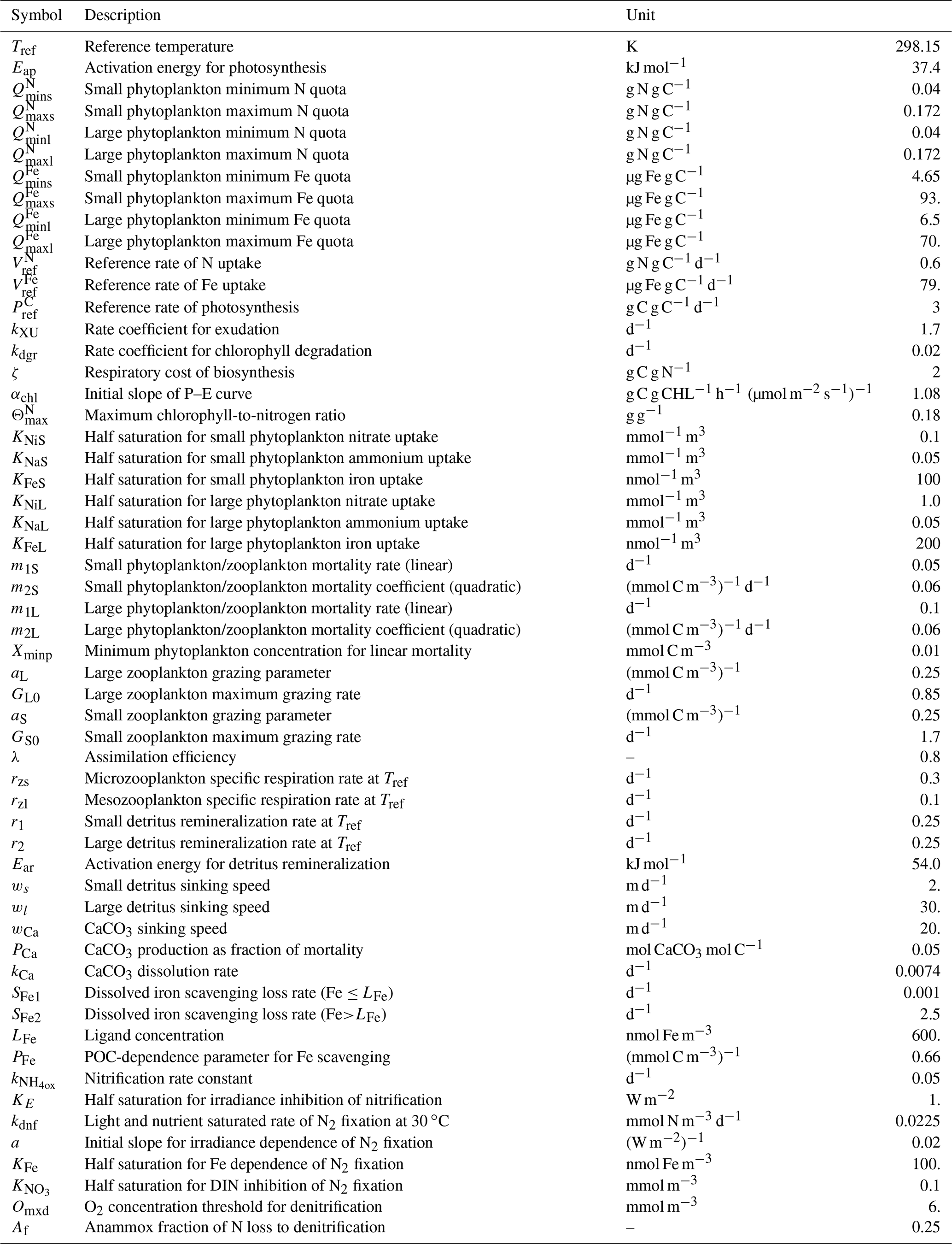
The CanOE biology model is based on the cellular regulation model of Geider et al. (1998). There are two phytoplankton size classes, and each group has four state variables: C, N, Fe, and chlorophyll. Photosynthesis is decoupled from cell production and photosynthetic rate is a function of the cell's internal N and Fe quotas. Each functional group has a specified minimum and maximum N quota and Fe quota, and nutrient uptake ceases when the maximal cell quota is reached. Chlorophyll synthesis is a function of N uptake and increases at low irradiance. There are also two size classes each of zooplankton and detritus. Small zooplankton graze on small phytoplankton, while large zooplankton graze on both large phytoplankton and small zooplankton. Small detritus sinks at 2 m d−1 and large detritus at 30 m d−1 (in CanESM5, there is a single detrital pool with a sinking rate of 8 m d−1). Model parameters and their values are listed in Table 1. A schematic of the model is shown in Fig. 1.
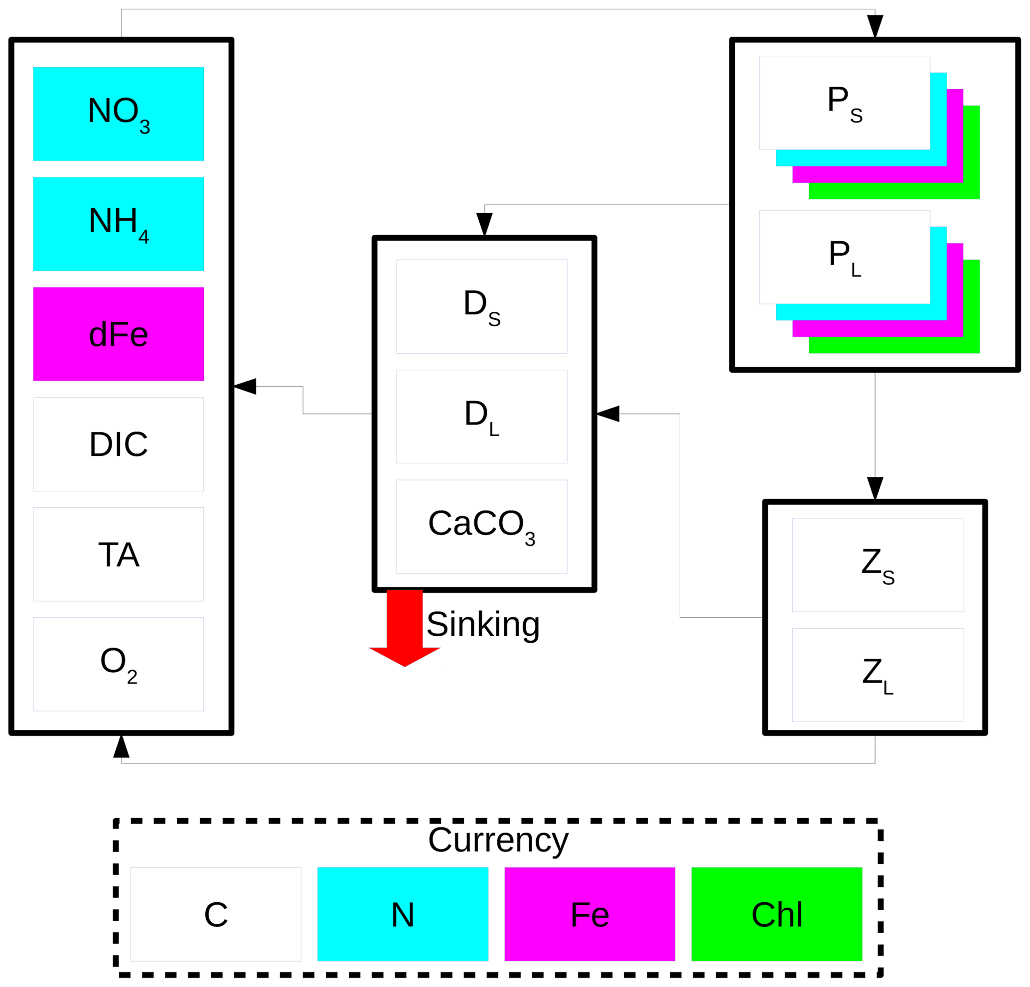
Figure 1Schematic of the CanOE biology model. Model currencies including chlorophyll (Chl) are indicated by coloured boxes except oxygen (O2) and carbonate (CaCO3). Arrows indicate flows of carbon (C), nitrogen (N), and iron (Fe) between compartments containing small (S) and large (L) phytoplankton (P), zooplankton (Z), and detritus (D) components; counterflows of oxygen are not shown.
2.1 Photosynthesis and phytoplankton growth
For simplicity and clarity, the equations are shown here for a single phytoplankton species and do not differ structurally for small and large phytoplankton. Some parameter values differ for the two phytoplankton groups; all parameter values are listed in Table 1.
Temperature dependence of photosynthetic activity is expressed by the Arrhenius equation:
where Eap is an enzyme activation energy that corresponds approximately to that of RuBisCo (see Raven and Geider, 1988), R is the gas constant (8.314 J mol−1 K−1), and temperature T and reference temperature Tref are in Kelvin. Maximal rates of nutrient (either N or Fe but generically referred to here with the superscript X) uptake are given by
where is the maximal uptake rate in mg of nutrient X per mg of cell C, X can represent N or Fe, Q is the nutrient cell quota and Qmin and Qmax its minimum and maximum values, and is a (specified) basal rate at T=Tref and Q=Qmin. These maximum rates are then reduced according to the ambient nutrient concentration, i.e.
where and , with Ni and Na indicating nitrate and ammonium respectively, and
where X indicates large or small phytoplankton (Table 1). The maximal carbon-based growth rate is given by
where is the rate at the reference temperature Tref under nutrient-replete conditions (Q=Qmax). The light-limited growth rate is then given by
where E is irradiance and θC is the chlorophyll-to-carbon ratio. The rate of chlorophyll synthesis is
These rates are then used to define a set of state equations for phytoplankton carbon (Cp), nitrogen (Np), iron (Fep), and chlorophyll (M).
where ζ is the respiratory cost of biosynthesis, G is the grazing rate (Eq. 12), CXS is the excess (above the ratio in grazer biomass) carbon in grazing losses (see Eq. 16a below), m1 and m2 are coefficients for linear and quadratic nonspecific mortality terms, CINTR is the concentration of intracellular carbohydrate carbon in excess of biosynthetic requirements, and kXU is a rate coefficient for its exudation to the environment. The nonspecific mortality terms are set to 0 below 0.01 mmol C m−3 to prevent biomass from being driven to excessively low levels in the high latitudes in winter; linear mortality terms can result in biomass declining to levels from which recovery would take much longer than the brief Arctic summer (Hayashida, 2018). The full equations for phytoplankton N, Fe, and chlorophyll are
where kdgr is a rate coefficient for nonspecific losses of chlorophyll e.g. by photooxidation, in addition to losses to grazing and other processes that also affect Cp, Np, and Fep. NXS and FeXS are remineralization of “excess” (relative to grazer or detritus ratios) N or Fe and are defined below (Eq. 16).
2.2 Grazing and food web interactions
Grazing rate depends on the phytoplankton carbon concentration, which most closely represents the food concentration available to the grazer (Elser and Urabe 1999; Loladze et al. 2000). Zooplankton biomass is also in carbon units. State equations for small and large zooplankton are
where
for small and large zooplankton, respectively, GZ is grazing of small zooplankton by large zooplankton, R is respiration, and m1 and m2 are non-grazing mortality rates. Large zooplankton grazing is divided into grazing on large phytoplankton and small zooplankton in proportion to the relative abundance of each:
Zooplankton biomass loss to respiration is given by
and uses the same activation energy as photosynthesis. Respiration (R) is assumed to consume only carbon and not result in catabolism of existing biomass when “excess” carbon is available in the prey. In addition, conservation of mass must be maintained by recycling to the dissolved pool grazer consumption of elements in excess of biosynthetic requirements when grazer and prey elemental ratios differ. In the case where the nutrient quota (relative to carbon) exceeds the grazer fixed ratio, the excess nutrient is remineralized to the dissolved inorganic pool. In the case where the nutrient quota is less than the grazer ratio, the grazer intake is reduced to what can be supported by the least abundant nutrient (relative to the grazer biomass ratio) and excess carbon is remineralized. For the case of two nutrients (in this case N and Fe), it is necessary to define
where G is equal to GS (Eq. 12a) for small zooplankton and GP (Eq. 13a) for large zooplankton, and RXY indicates the fixed ratio of element X to element Y in grazer biomass. The “excess” carbon available for respiration is
and the excess nutrients remineralized to their inorganic pools are
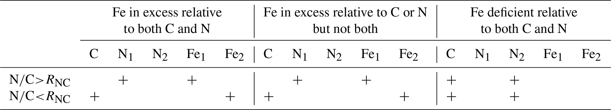
where is a switch to prevent double counting in cases where one of the terms is redundant (the excess relative to the least abundant element is included in the other term) but would otherwise be nonzero (Δ is a constant equal to 10−15, to prevent division by zero). For three elements, there are 3! = 6 possible cases: for N greater or less than CPRNC, Fe may be either in excess relative to both C and N, deficient relative to both, or in excess relative to one but not the other (Table 2).
Table 2Cases where the “excess” terms are nonzero. These terms are always greater than or equal to zero, and always zero when the phytoplankton elemental ratio is equal to the grazer biomass ratio. A plus (+) sign indicates that a specific term is positive. N1 and N2, Fe1 and Fe2 indicate the first and second terms in Eq. (16b) and (16c). RNC is the grazer (Redfield) ratio.
2.3 Organic and inorganic pools
There are two pools of detritus with different sinking rates but the same fixed elemental ratios. Detrital C/N/Fe ratios are the same as zooplankton, so zooplankton mortality or grazing of small zooplankton by large zooplankton produce no “excess”. Phytoplankton mortality, and defecation by zooplankton grazing on phytoplankton, produces excess nutrient or excess C that needs to be recycled into the inorganic pool in a similar fashion as outlined above for the assimilated fraction of grazing on phytoplankton.
The conservation equations for detrital C are
where Tg is an Arrhenius function for temperature dependence of remineralization and w is the sinking speed. The conservation equations for inorganic C, N, and Fe are
where Nox is microbial oxidation of ammonium to nitrate (nitrification), Ndnf and Ndentr are sources and sinks associated with dinitrogen fixation and denitrification, and Af is the ammonium fraction of denitrification losses, associated with anaerobic ammonium oxidation (“anammox”). The oxygen equation is essentially the inverse of Eq. (18a), with additional terms for oxidation and reduction of N, i.e.
Nitrification is given by
where E(z) is the layer mean irradiance at depth z. Dinitrogen fixation is parameterized as an external input of ammonium dependent on light, temperature and Fe availability, and inhibited by high ambient concentrations of inorganic N:
where Tdnf=max(0, 1.962(Tf−0.773)), i.e. a linear multiple of Eq. (1) that is 0 at T<20 ∘C and unity at T=30 ∘C. The temperature, iron, and light limitation terms are based on Pelagic Interactions Scheme for Carbon and Ecosystem Studies (PISCES) (Aumont et al,, 2015); the N-inhibition term is from CMOC (Zahariev et al., 2008) (CMOC implicitly combines nitrate and ammonium into a single inorganic N pool).
Denitrification is parameterized as a fraction of total remineralization that increases as a linear function of oxygen concentration for concentrations less than a threshold concentration Omxd:
Remineralization is then divided among oxygen (1−Nfrxn), nitrate (0.875Nfrxn), and ammonium (0.125Nfrxn) assuming an average anammox contribution of 25 % (Babbin et al., 2014). We use this average ratio of anammox to classical denitrification to partition fixed N losses between NO and NH; the DIC sink and organic matter source associated with anammox are small and are neglected here.
2.4 Calcification, calcite dissolution, and alkalinity
In CanOE, calcification is represented by a prognostic detrital calcite pool with its own sinking rate (distinct from that of organic detritus), and calcite burial or dissolution in the sediments depends on the saturation state (100 % burial when ΩC≥1, 100 % dissolution when ΩC<1). Calcification is represented by a detrital calcium carbonate (CaCO3) state variable, but no explicit calcifier groups. Detrital CaCO3 sinks in the same fashion as detrital particulate organic carbon (POC), with a sinking rate independent of those for large and small organic detritus. Calcite production is represented as a fixed fraction of detritus production from small phytoplankton and small zooplankton mortality:
Calcite dissolution occurs throughout the water column as a first-order process (i.e. no dependence on temperature or saturation state). Approximately 80 % of calcite produced is exported from the euphotic zone. In CanESM5-CanOE, burial in the sediments is represented as a simple “on/off” switch dependent on the calcite saturation state (zero when ΩC<1 and 1 when ΩC≥1). In CanESM5, calcification is parameterized by a temperature-dependent “rain ratio” (Zahariev et al., 2008), and 100 % burial of calcite that reaches the seafloor is assumed. Calcite burial in both models is balanced by an equivalent source of DIC and alkalinity at the ocean surface (in the same vertical column) as a crude parameterization of fluvial sources.
For each mole of calcite production, two moles of alkalinity equivalent are lost from the dissolved phase; the reverse occurs during calcite dissolution. There are additional sources and sinks for alkalinity associated with phytoplankton nutrient (NH, NO) uptake, organic matter remineralization, nitrification, denitrification, and dinitrogen fixation (Wolf-Gladrow et al., 2007; see Table S2 in the Supplement). The anammox reaction does not in itself contribute to alkalinity (Jetten at al., 2001), but there is a sink associated with ammonium oxidation to nitrite (the model does not distinguish between nitrite and nitrate). Autotrophic production of organic matter by anammox bacteria is a net source of alkalinity (Strous et al., 1998), but this source is extremely small (∼ 0.03 mol molN−1) and is neglected here. Globally, the sources and sinks of alkalinity from the N cycle offset each other such that there is no net gain or loss as long as the global fixed N pool is conserved (see Sect. 2.5 below). If dinitrogen fixation and denitrification are allowed to vary freely, there will generally be a net gain or loss of fixed N and therefore of alkalinity.
2.5 External nutrient sources and sinks
External sources and sinks consist of river inputs, aeolian deposition, biological N2 fixation, denitrification, mobilization of Fe from reducing sediments, loss of Fe to scavenging, and burial of calcium carbonate in the sediments. There is no burial of organic matter; organic matter reaching the seafloor is instantaneously remineralized. Aeolian deposition of Fe is calculated from a climatology of mineral dust deposition generated from offline (atmosphere-only) simulations with CanAM4 (von Salzen et al., 2013), with an Fe mass fraction of 5 % and a fractional solubility of 1.4 % in the surface layer. Subsurface dissolution is parameterized based on PISCESv2 (Aumont et al., 2015); the total dissolution is 6.35 %, with 22 % of soluble Fe input into the first vertical layer (see the Supplement). Iron from reducing sediments is also based on PISCES, with a constant areal flux of 1000 nmol m−2 d−1 in the first model level, declining exponentially with increasing seafloor depth (i.e. assuming that shelf sediments are the strongest source and the sediments become progressively more oxygenated with increasing seafloor depth) with an e-folding length scale of about 600 m. Scavenging of dissolved iron is first order with a high rate (2.5 d−1) for concentrations in excess of 0.6 nM (Johnson et al., 1997). For concentrations below this threshold, the rate is much lower (0.001 d−1) and is weighted by the concentration of organic detritus (Christian et al., 2002b), i.e.
where Fe is the dissolved iron concentration, DS and DL are the small and large detritus concentrations, SFe1 is the first-order scavenging rate in surface waters with abundant particulates, and PFe is an empirical parameter to determine the dependence on particle concentration (Table 1). The basis for this parameterization is that the rate of scavenging must depend not only on the concentration of iron but on the concentration of particles available for it to precipitate onto and assumes that detrital POC is strongly positively correlated with total particulate matter. Scavenging is treated as irreversible; i.e. scavenged Fe is not tracked and does not re-enter the dissolved phase.
N2 fixation and denitrification vary independently in CanOE, so the global total N pool can change. Conservation is imposed by adjusting the global total N pool according to the difference between the gain from N2 fixation and the loss to denitrification. A slight adjustment is applied to the nitrate concentration at every grid point, while preserving the overall spatial structure of the nitrate field. Adjustments are multiplicative rather than additive to avoid producing negative concentrations. This adjustment does not maintain (to machine precision) a constant global N inventory but is intended to minimize long-term drift, keeping it much smaller than the free surface error (see below). This adjustment is applied every 10 d and has a magnitude of approximately of the total N.
When the total fixed N adjustment is applied, one mole of alkalinity is added (removed) per mole of N removed (added), to account for the alkalinity sources associated with N2 fixation (creation of new NH) and denitrification (removal of NO) (Wolf-Gladrow et al., 2007; see Table S2 in the Supplement). As there is a 2 mol molN−1 sink associated with nitrification, this formulation is globally conservative. As noted above, in CanOE CaCO3 can dissolve or be buried in the sediments depending on the calcite saturation state. DIC and alkalinity lost to burial are reintroduced at the ocean surface, at the same grid point as burial occurs, providing a crude parameterization of river inputs so that global conservation is maintained (fresh water runoff contains no DIC or alkalinity). However, the OPA free surface formulation is inherently imperfect with regard to tracer conservation. Drift in total ocean alkalinity and nitrogen over time is on the order of 0.01 % and 0.03 % per thousand years, respectively.
2.6 Ancillary data
For first-order model validation, we have relied largely on global gridded data products rather than individual profile data. Global gridded data from World Ocean Atlas 2018 (WOA2018) (Locarnini et al., 2018; Zweng et al., 2018; Garcia et al., 2018a, 2018b) were used for temperature, salinity, and oxygen and nitrate concentration. DIC and alkalinity were taken from the GLODAPv2.2016b gridded data product (Key et al., 2015; Lauvset et al., 2016). Offline carbon chemistry calculations were done following the Best Practices Guide (Dickson et al., 2007) and the OMIP-BGC protocols (Orr et al., 2017), and they are identical to those used in the models except that constant reference concentrations were used for phosphate (1 µM) and silicate (10 µM).
There is no global gridded data product for Fe, but we have made use of the GEOTRACES Intermediate Data Product 2017 (Schlitzer et al., 2018), and the data compilations from Monterey Bay Aquarium Research Institute (MBARI) (Johnson et al., 1997; 2003) and North Pacific Marine Science Organization (PICES) Working Group 22 (Takeda et al., 2013). The latter two are concentrated in the Pacific, while GEOTRACES is more global. The combined data sets provide more than 10000 bottle samples from more than 1000 different locations (Fig. S10a in the Supplement) (excluding some surface transect data that involve frequent sampling of closely spaced locations along the ship track). More details about model comparison to these data compilations and the list of original references are given in the Supplement.
Satellite ocean colour estimates of surface chlorophyll were taken from the combined SeaWiFS/MODIS climatology described by Tesdal et al. (2016). Climatological satellite POC was downloaded from the NASA Ocean Color website and is based on the algorithm of Stramski et al. (2008) using MODIS Aqua data. This climatology differs slightly from the chlorophyll one in terms of years included and sensors utilized, but as only climatological concentrations are considered and each climatology covers ∼ 15 years, these differences will have negligible effect on the results presented. Satellite chlorophyll concentrations greater than 1 mg m−3 were excluded as these are mostly associated with coastal regions not resolved by coarse-resolution global ocean models.
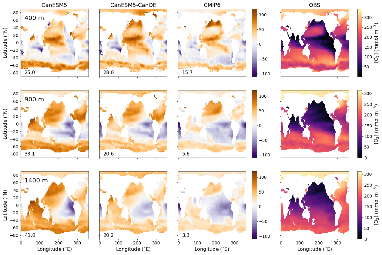
Figure 2Global distribution of oxygen (O2) concentration in mmol m−3 at 400, 900, and 1400 m (rows) for CanESM5-CanOE, CanESM5, the mean for other (non-CanESM) CMIP6 models, and World Ocean Atlas 2018 (WOA2018) observations (columns). Numbers on the lower left are the mean model bias. Differences from the observation-based fields are shown in Fig. S2 in the Supplement.
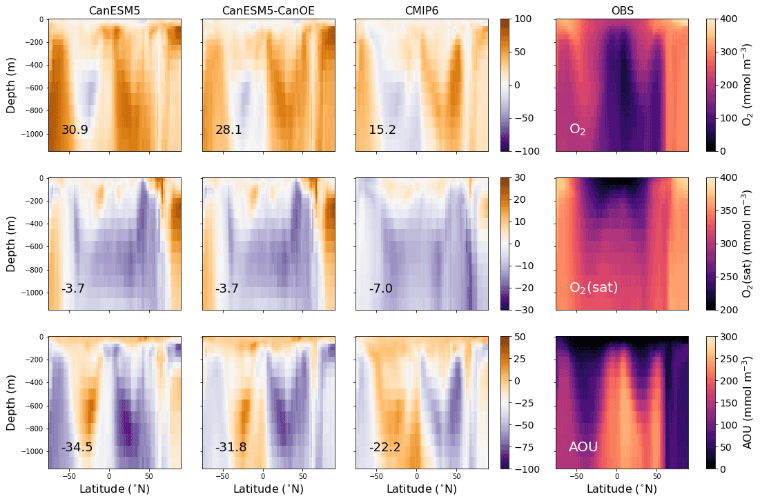
Figure 3Latitude–depth distribution (surface to 1750 m) of zonal mean oxygen concentration (O2), oxygen concentration at saturation (O2(sat)), and apparent oxygen utilization (AOU) in mmol m−3 for CanESM5-CanOE, CanESM5, the mean for other CMIP6 models, and observations (WOA2018). Note different colour scales for different rows. Numbers on the lower left are the mean model bias. Differences from the observation-based fields are shown in Fig. S2 in the Supplement.
CMIP6 model data were regridded by distance-weighted averaging using the Climate Data Operators (https://code.mpimet.mpg.de/projects/cdo/, last access: 19 May 2022) to a common grid (2×2∘, 33 levels) to facilitate ensemble averaging. The vertical levels used are those used in GLODAP and in earlier (through 2009) versions of the World Ocean Atlas (e.g. Locarnini et al., 2010). For large-scale tracer distributions, using a 1 or 2∘ grid makes little difference (for example, the spatial pattern correlation between CanESM5 and observed oxygen concentration at specific depths on a 1 or 2∘ grid differs by an average of 0.0011). The years 1986–2005 of the historical experiment were averaged into climatologies or annual means, for meaningful comparison with observation-based data products. The CMIP6 historical experiment runs from 1850–2014 with atmospheric CO2 concentration (and other atmospheric forcings) based on historical observed values. A single realization was used in each case (see Table S3); 20-year averages are used to minimize the effect of internal variability (e.g. Arguez and Vose, 2011; see Table S4). Where time series are shown, 5-year means are used.
Sampling among CMIP6 models was somewhat opportunistic, and the exact suite of models varies among the analyses presented. When we conducted a search for a particular data field, we included in the search parameters all models that published that field and repeated the search at least once for models that were unavailable the first time the search was executed. In some cases, model ensemble means excluded all but one model from a particular “family” (e.g. there are three different MPI-ESM models for which ocean biogeochemistry fields were published), as the solutions were found to be similar and would bias the ensemble mean towards their particular climate. The models used are ACCESS-ESM1-5, CESM2, CESM2-WACCM, CNRM-ESM2-1, GFDL-CM4, GFDL-ESM4, IPSL-CM6A-LR, MIROC-ES2L, MPI-ESM-1-2-HAM, MPI-ESM1-2-LR, MPI-ESM1-2-HR, MRI-ESM2-0, NorESM2-LM, NorESM2-MM, and UKESM1-0-LL. Details of which variables and realizations are used for which models are given in Table S3 in the Supplement.
We first describe the large-scale distribution of oxygen, DIC, alkalinity, and the saturation state with respect to CaCO3 that derives from these large-scale tracer distributions. Tracer distributions result partly from ocean circulation and partly from biogeochemical processes. An overall evaluation of the ocean circulation model is given in Swart et al. (2019a). Analyzing CanESM5 and CanESM5-CanOE (with identical circulation) as well as CanESM2 where possible (same biogeochemistry as CanESM5 but different circulation) allows us to separate the effects of physical circulation and biogeochemistry on evolving model skill with respect to large-scale tracer distributions. In subsequent sections, we address the main areas where CanESM5 and CanESM5-CanOE differ, such as the interaction of the iron and nitrogen cycles and plankton community structure. Finally, we present some temporal trends over the course of the historical experiment (1850–2014).
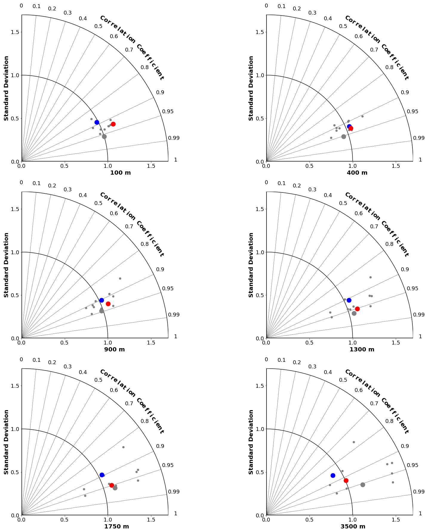
Figure 4Taylor diagrams (Taylor, 2001) comparing modelled and observed distributions of oxygen at specific depths from 100 to 3500 m. The angle from the vertical indicates spatial pattern correlation. Distance from the origin indicates ratio of standard deviation in modelled vs. observed (WOA2018) fields. Red dots represent CanESM5-CanOE, blue dots CanESM5, small grey dots other CMIP6 models, and large grey dots the model ensemble mean for all CMIP6 models except CanESM5 and CanESM5-CanOE.
3.1 Distribution of oxygen
The spatial distribution of oxygen concentration ([O2]) at selected intermediate depths (400, 900, and 1400 m) is shown in Fig. 2 for gridded data from WOA2018 and differences from that observational data product for CanESM5, CanESM5-CanOE, a model ensemble mean (MEM) of CMIP6 models (excluding CanESM5 and CanESM5-CanOE). The depths were chosen to span the depth range where low oxygen concentrations exist; these low-oxygen environments are of substantial scientific and societal interest and are sensitive to model formulation. The major features are consistent across the models. Both CanESM models as well as the MEM show elevated oxygen concentrations relative to observations, particularly in the North Pacific, the North Atlantic, and the Southern Ocean. In the Indian Ocean, both CanESM models show high oxygen concentrations in the Arabian Sea and deeper layers of the Bay of Bengal relative to observations and the MEM; these biases are somewhat smaller in CanESM5-CanOE than in CanESM5 (Fig. 2).
The ocean's oxygen minimum zones (OMZs) are mostly located in the eastern Pacific Ocean, the northern North Pacific, and the northern Indian Ocean; the spatial pattern changes with increasing depth (Fig. 2), but the OMZs are mostly located between 200 and 2000 m depth. Biases in the EBC regions are depth and model specific. CanESM5 shows particularly strong oxygen depletion at 1400 m in the eastern tropical Pacific. In the southeastern Atlantic, models tend to be biased low at the shallower depths and show somewhat more variation at greater depths (Fig. 2). Overall, [O2] biases tend to be positive over large areas of ocean with the exception of some EBC regions, implying that models exaggerate the extent to which remineralization is concentrated in these regions. An alternate version of Fig. 2 that shows the modelled concentrations is given in Fig. S2 in the Supplement.
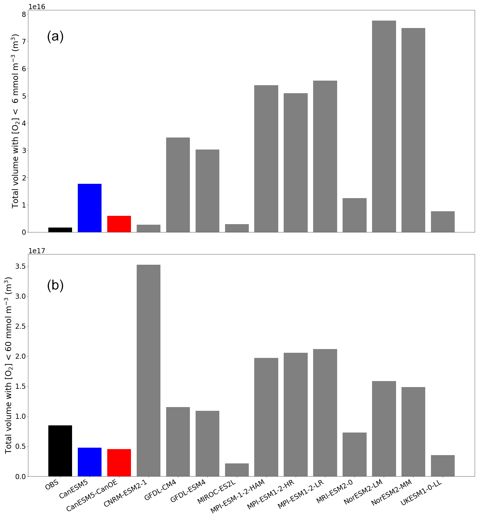
Figure 5Total volume of ocean with oxygen (O2) concentration less than (a) 6 mmol m−3 (mean for last 30 years of the historical experiment) and (b) 60 mmol m−3. Observation are from WOA2018.
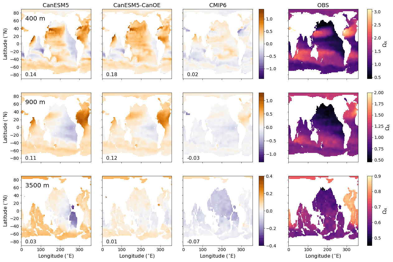
Figure 6Global distribution of aragonite saturation (ΩA) at 400, 900, and 3500 m for CanESM5-CanOE, CanESM5, the mean for other CMIP6 models, and observations (GLODAPv2 and WOA2018). Note different colour scales for different depths. Numbers on the lower left are the mean model bias. Differences from the observation-based fields are shown in Fig. S2 in the Supplement.
The zonal mean oxygen concentration, saturation concentration, and apparent oxygen utilization (AOU) are shown in Fig. 3 for the same four cases. Again, the models generally show a positive bias in [O2], particularly in high-latitude deep waters. The major ocean circulation features are reproduced fairly well in all cases (e.g. weaker ventilation of low-latitude subsurface waters, greater vertical extent of well-ventilated surface waters in the subtropics). The saturation concentration (a function of temperature and salinity) generally shows relatively little bias, implying that the bias in [O2] arises mainly from remineralization and/or ventilation. AOU is lower than observed over much of the subsurface ocean. CanESM5 and CanESM5-CanOE show a high bias over much of the Northern Hemisphere that reflects the high concentrations in the North Pacific and North Atlantic (Fig. 2). The overall trend of bias with latitude in CanESM5 and CanESM5-CanOE is generally similar to the MEM, but the biases are larger. The bias in CanESM5 is generally slightly larger than in CanESM5-CanOE, except in the Arctic Ocean. Again, Fig. S2 in the Supplement includes a version of this plot that shows the modelled concentration fields.
The skill of each model with respect to the distribution of O2 at different depths is represented by Taylor diagrams (Taylor, 2001) in Fig. 4. These diagrams allow us to assess how well the model reproduces the spatial distribution at a range of depths, because different physical and biogeochemical processes determine the distribution in different depth ranges. All of the CMIP6 models that were shown as an ensemble mean in Figs. 2 and 3 are shown individually. The large blue dots represent CanESM5, red CanESM5-CanOE, and grey the MEM; the smaller grey dots represent the individual models. CanESM5-CanOE shows slightly higher pattern correlation than CanESM5 at all depths. Both models compare favourably with the full suite of CMIP6 models, with r>0.85 for CanESM5 and r>0.9 for CanESM5-CanOE at all depths examined, and a normalized standard deviation within ±25 % of unity.
The total volume of ocean with [O2] less than 6 mmol m−3 (the threshold for denitrification; Devol, 2008) and 60 mmol m−3 (a commonly used index of hypoxia) is shown in Fig. 5. The total volume is highly variable among models (note, however, that there are several clusters of related models with quite similar totals). CanESM5 and CanESM5-CanOE have among the lowest total volumes (i.e. the interior ocean is relatively well ventilated) and are among the nearest to the observed total. For [O2]<60 mmol m−3 the bias is, nonetheless, quite large (i.e. the observed volume is underestimated by almost 50 % in both models). The volume of water with [O2] below the denitrification threshold is overestimated in both CanESM5 and CanESM5-CanOE; CanESM5-CanOE has a much smaller total that is closer to the observed value. The bias in the spatial pattern of hypoxia (not shown) is generally similar to the bias in dissolved oxygen distribution (Fig. 2). The low-oxygen regions are generally more concentrated in the eastern tropical Pacific in the models than in observations, and the low-oxygen region in the northwest Pacific is not well reproduced in CanESM models.
3.2 Distribution of DIC, alkalinity, and CaCO3 saturation
The spatial distribution of aragonite saturation state (ΩA) at selected depths is shown in Fig. 6. The first two depths are the same as in Fig. 2, but a much greater depth is also included, as the length scale for CaCO3 dissolution is greater than for organic matter remineralization. In this case, the observations are a combination of GLODAPv2 (Key et al., 2015; Lauvset et al., 2016) for DIC and alkalinity, and WOA2018 for temperature and salinity. CanESM5 and CanESM5-CanOE show an overall high saturation bias at the shallower depths, particularly in the North Atlantic, with a low bias found mainly in the eastern Pacific. The low saturation bias in the eastern tropical Pacific is substantially reduced in CanESM5-CanOE compared to CanESM5. On the other hand, CanESM5 generally does better than CanESM5-CanOE, or the MEM, at reproducing the low saturation states in the northwestern Pacific and the Bering Sea. Both CanESM models show a high saturation state bias in the North Atlantic and the well-ventilated regions of the north Pacific subtropical gyre; these biases are slightly smaller in CanESM5-CanOE. Maps of the calcite and aragonite saturation horizon (Ω=1) depth are shown in Fig. S3 in the Supplement; these generally confirm the same biases noted in Fig. 6.
Zonal mean distributions of aragonite saturation state (ΩA), calcite saturation state (ΩC), and carbonate ion concentration ([CO]) and the differences of the models from the observations are shown in Fig. 7 (Fig. S2 in the Supplement includes versions of Figs. 6 and 7 that show the modelled fields). The models generally compare well with the observations in the representation of the latitude–depth distribution of high- and low-saturation waters. CanESM5 has a high saturation bias in low-latitude surface waters that is somewhat reduced in CanESM5-CanOE. Both CanESM5 models show a high saturation bias in Northern Hemisphere intermediate (e.g. 200–1000 m) depth waters that is larger than in the MEM. This is primarily a result of low Ω in the North Atlantic Ocean (Fig. 6).

Figure 7Latitude–depth distribution of zonal mean (surface to 1150 m) aragonite saturation state (ΩA), calcite saturation state (ΩC), and carbonate ion concentration ([CO]) in mmol m−3 for CanESM5-CanOE, CanESM5, the mean for other CMIP6 models, and observations (GLODAPv2 and WOA2018). Numbers on the lower left are the mean model bias. Differences from the observation-based fields are shown in Fig. S2 in the Supplement.
Taylor diagrams for a range of depths are shown for DIC in Fig. 8 and for ΩA in Fig. 9 (for alkalinity; see Fig. S4 in the Supplement). As expected, the MEM generally compares favourably with the individual models (e.g. Lambert and Boer, 2001). CanESM5 and CanESM5-CanOE compare favourably with the full suite of CMIP6 models. CanESM5-CanOE shows a gain in skill relative to CanESM5, and both show improvement relative to CanESM2. At 400 m, CanESM2 stands out as having extremely high variance, which is mostly due to extremely high DIC concentrations occurring over a limited area in the eastern equatorial Pacific (not shown). This bias is present in CanESM5 and in CMIP6 models generally (Fig. 6) but involves much lower concentrations spread over a larger area.
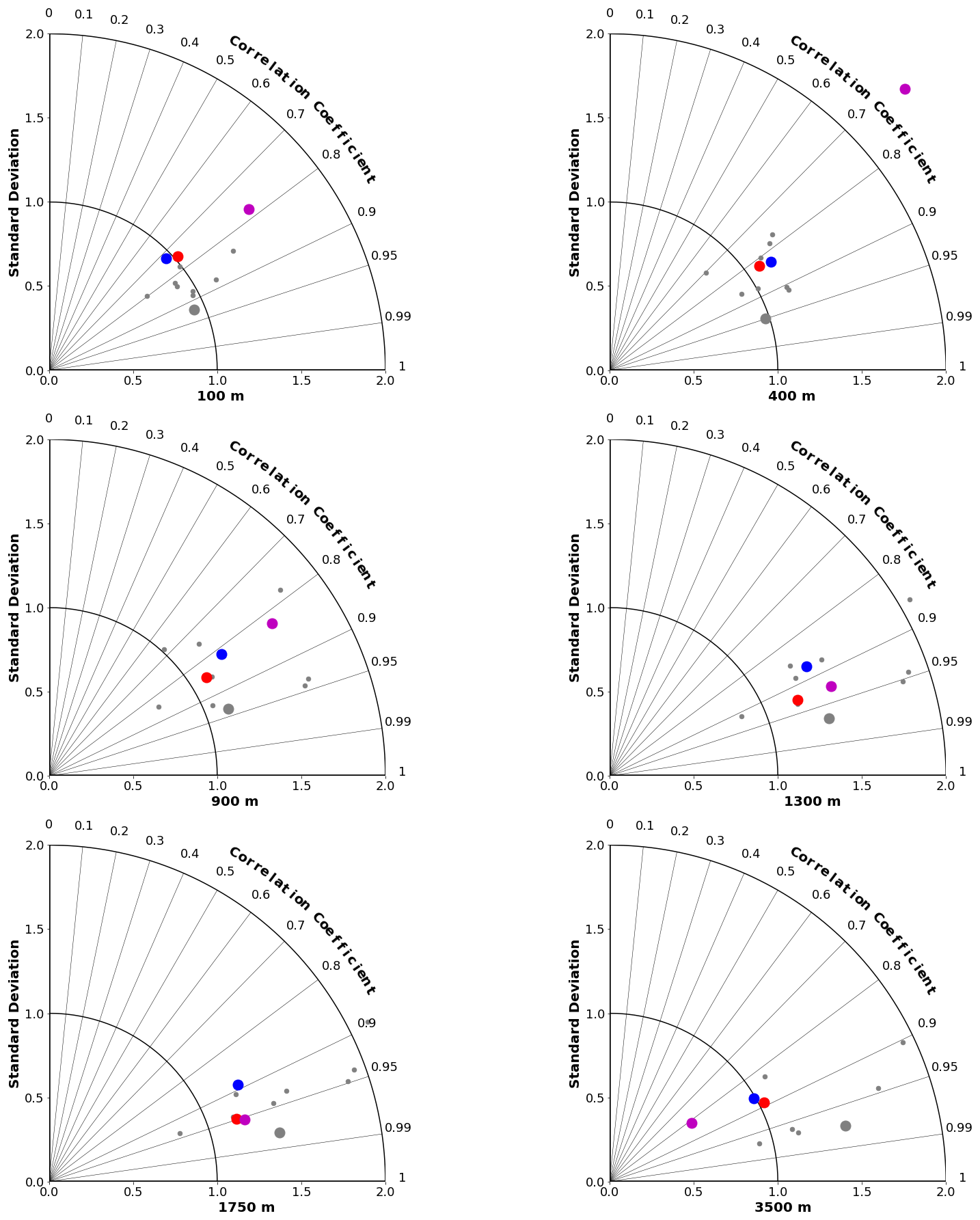
Figure 8Taylor diagrams comparing modelled and observed distributions of DIC at specific depths from 100 to 3500 m. Observations are from GLODAPv2 (Lauvset et al., 2016). Red dots represent CanESM5-CanOE, blue dots CanESM5, magenta dots CanESM2, small grey dots other CMIP6 models, and large grey dots the model ensemble mean for all CMIP6 models except CanESM5 and CanESM5-CanOE.
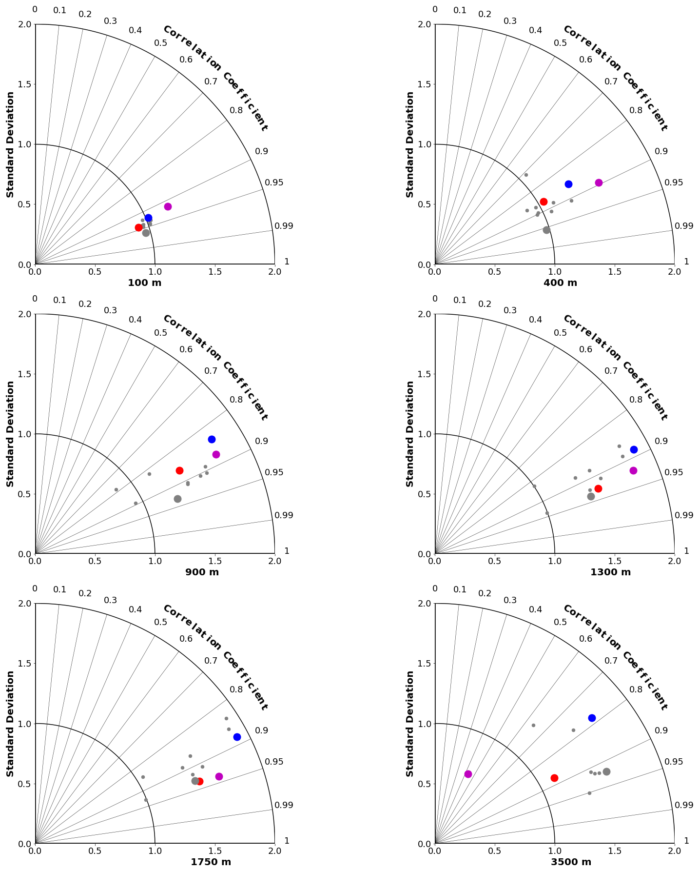
Figure 9Taylor diagrams comparing modelled and observed (GLODAPv2 and WOA2018) distributions of ΩA at specific depths from 100 to 3500 m. Symbol colours are as in Fig. 8.
3.3 N and Fe cycles
An important difference between CanESM5 and CanESM5-CanOE is the inclusion of a prognostic Fe cycle. The CMOC iron mask (Zahariev et al., 2008) was a pragmatic solution in the face of resource limitations but is inherently compromised as it can not evolve with a changing climate. The first-order test of a model with prognostic, interacting Fe and N cycles is whether it can reproduce the distribution of HNLC regions and the approximate surface macronutrient concentrations within these. CanESM5-CanOE succeeded by this standard, although the surface nitrate concentrations are biased low in the subarctic Pacific and equatorial Pacific and high in the Southern Ocean and in the global mean (Fig. 10).
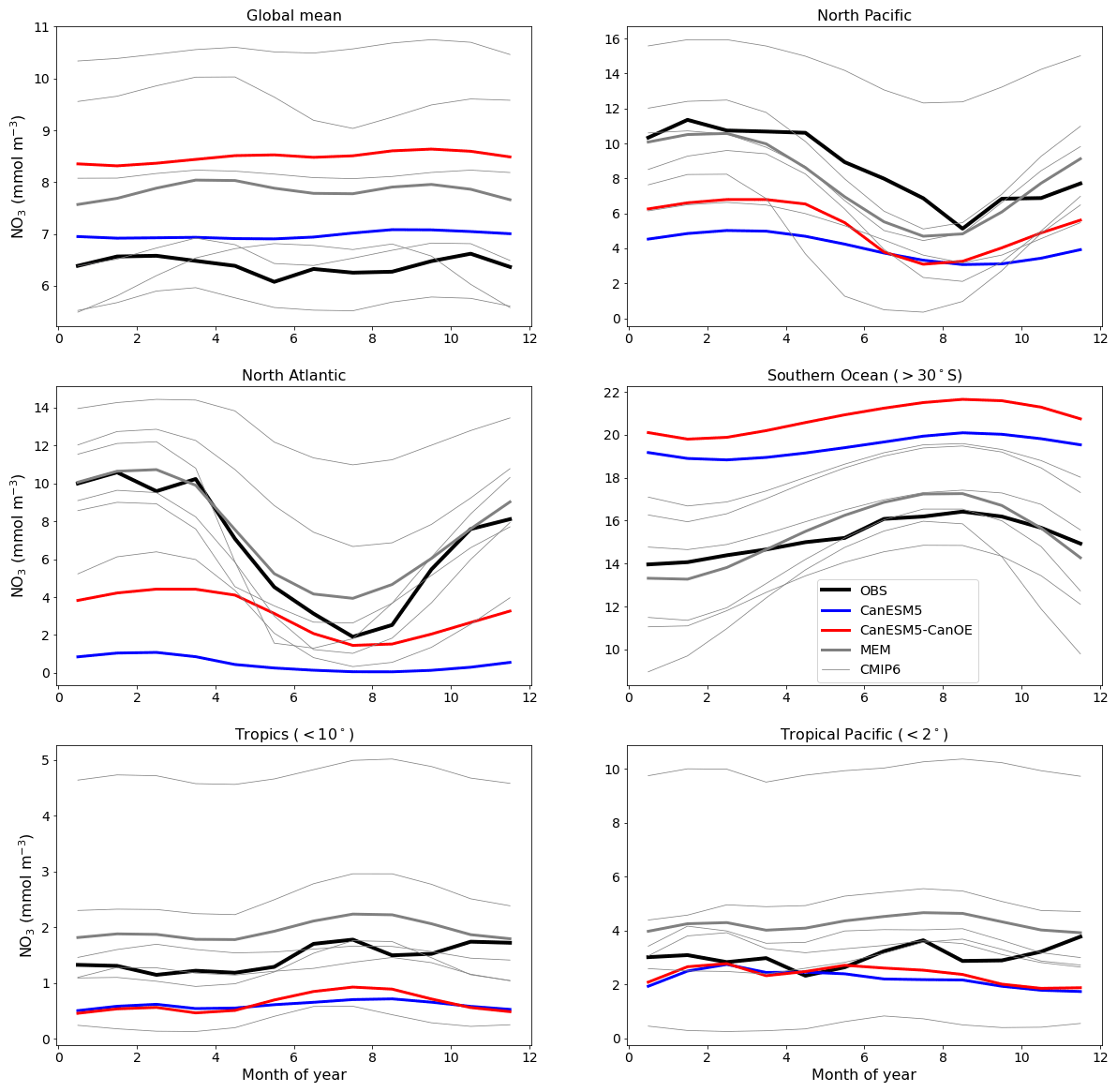
Figure 10Climatological seasonal cycle of surface nitrate concentration averaged for selected ocean regions. The thick red line represents CanESM5-CanOE, thick blue line CanESM5, thick black line observations (WOA2018), thin grey lines individual CMIP6 models, and thick grey line the model ensemble mean (excluding CanESM5 and CanESM5-CanOE). Regional boundaries are given in Table S5 and Fig. S5.
The seasonal cycle of the zonal mean surface nitrate concentration for a selection of CMIP6 models is shown in Fig. 11. CanESM5, CanESM5-CanOE, and CNRM-ESM2-1 reproduce the equatorial enrichment and the low concentrations in the tropical–subtropical latitudes fairly well. Some models either have very weak equatorial enrichment (MPI-ESM1-2-LR) or too high a concentration in the off-equatorial regions (UKESM1-0-LL, NorESM2-LM). UKESM1-0-LL has very high concentrations throughout the low-latitude Pacific, which biases the ensemble mean (Fig. 11). Figure S6 in the Supplement shows the same data as Fig. 11 but for a more limited latitude range to better illustrate model behaviour in the tropics. CanESM5, CanESM5-CanOE, and CNRM-ESM2-1 reproduce the seasonal cycle of tropical upwelling (e.g. Philander and Chao, 1991), with highest concentrations in summer.
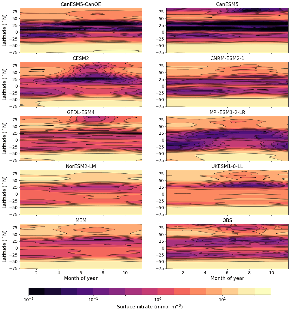
Figure 11Climatological seasonal cycle of zonal mean surface nitrate concentration for a selection of CMIP6 models, a model ensemble mean (MEM) excluding CanESM5 and CanESM5-CanOE, and an observation-based data product (WOA2018). An alternate version showing only latitudes <20∘ is given in Fig. S6.
The surface distribution of dissolved iron (dFe) in various CMIP6 models is shown in Fig. 12. For Fe there is no observation-based global climatology with which to compare the model solutions (some comparisons to available profile data are shown in Fig. S10b–h in the Supplement). CanESM5-CanOE shows a similar overall spatial pattern to other models, and generally falls in the middle of the spread, particularly regarding concentrations in the Southern Ocean. Several models show extremely high concentrations in the tropical–subtropical North Atlantic (Sahara outflow region). CanESM5-CanOE, along with CNRM-ESM2-1 and CESM2, has much less elevated concentrations in this region, due to lower deposition or greater scavenging or both. CanESM5-CanOE has its lowest concentration in the eastern subtropical South Pacific, which is common to many models (Fig. 12). The area of strong surface depletion is generally more spatially restricted in CanESM5-CanOE than in other models, and surface dFe concentrations are greater over large areas of the Pacific. Both the north–south and east–west asymmetry of distribution in the Pacific is greater in CanESM5-CanOE than in most other models, some of which show the South Pacific minimum extending westward across the entire basin, and others into the Northern Hemisphere. Only in CESM2 is this minimum similarly limited to the southeast Pacific.
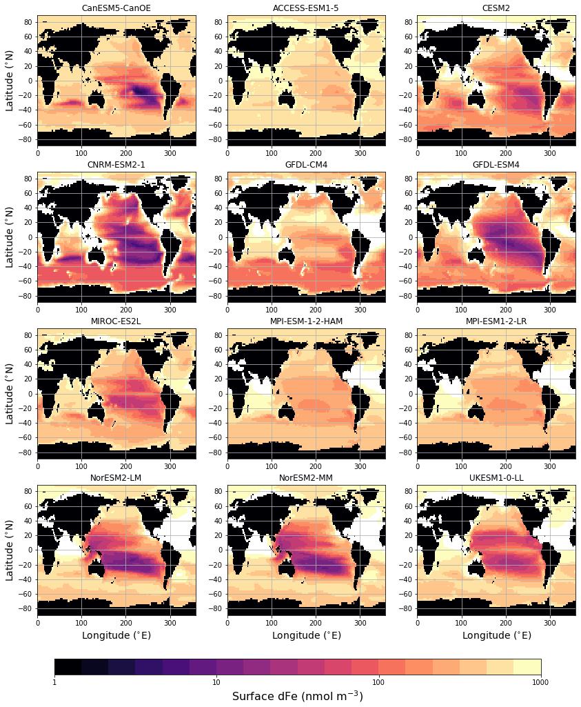
Figure 12Global distribution of dissolved iron (dFe) concentration (nmol m−3) at the ocean surface for CanESM5-CanOE and other CMIP6 models that published this field. Concentrations exceeding 1000 nmol m−3 are masked in white. CanESM5 is not included because it does not have prognostic iron.
The mean depth profiles of dFe are shown in Fig. 13. Some models show more of a “nutrient-type” (increasing with depth due to strong near-surface biological uptake and subsequent remineralization) profile, some a more “scavenged-type” (maximal at the surface, declining with depth) profile (see Li, 1991; Nozaki, 2001), and others a hybrid profile (increasing downward but with a surface enrichment). CanESM5-CanOE is at the “nutrient-type” end of spectrum with a generally monotonic increase with depth to a near-constant deep-water concentration of 0.6 nM and a very slight near-surface enrichment (see also Fig. S10b, c in the Supplement).
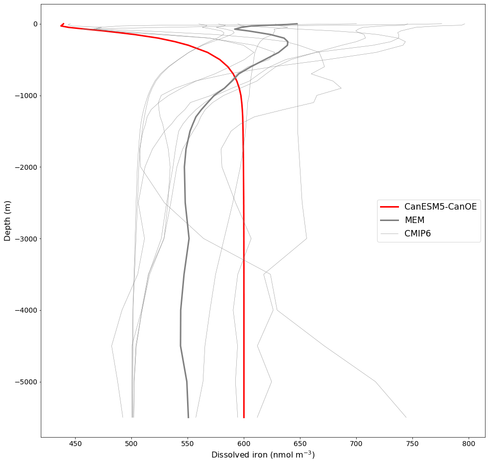
Figure 13Global mean depth profiles of dissolved iron concentration for CanESM5-CanOE and other CMIP6 models that published this field. GFDL-CM4 is excluded because it has very high concentrations (>2000 nmol m−3) near the surface. The thick red line represents CanESM5-CanOE, the thin grey lines individual CMIP6 models, and the thick grey line the model ensemble mean (excluding CanESM5-CanOE and GFDL-CM4).
Mean surface nitrate and dFe concentrations for selected ocean regions are shown in Fig. 14. CanESM5-CanOE shows concentrations that are within the range of CMIP6 models, although in some cases at the higher or lower end. Surface nitrate concentrations generally compare favourably with the observation-based climatology, but are biased low in HNLC regions other than the Southern Ocean. These biases are not necessarily a consequence of having too much or too little iron. For example, in the Southern Ocean CanESM5-CanOE has among the highest surface nitrate concentrations, but it also has some of the highest dFe concentrations, and the high nitrate bias is present in CanESM5 as well. Comparisons with the limited GEOTRACES data available suggest that near-surface dFe concentrations in the Southern Ocean are biased high rather than low in CanESM5-CanOE (not shown). One region where there does seem to be a strong correlation between surface nitrate and dFe concentrations is the western subarctic Pacific. All but two models (CNRM-ESM2-1, NorESM2-LM) fall along a spectrum from high Fe/low nitrate to low Fe/high nitrate. CanESM5-CanOE falls near the high Fe/low nitrate end of the range.
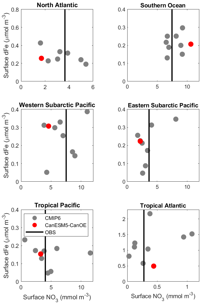
Figure 14Mean surface nitrate (NO3) vs. dissolved iron (dFe) concentrations in different oceans, including the major high-nutrient/low-chlorophyll (HNLC) regions. CanESM5-CanOE is shown as a red dot and other CMIP6 models as grey dots (CanESM5 is not included because it does not have iron). Observed NO3 is shown as a vertical black line as there are no observational estimates of dFe concentration. For GFDL-CM4, nitrate is estimated as phosphate ×16. Region definitions are given in Table S5 and Fig. S5.
Surface nitrate concentrations along the Pacific Equator during the upwelling season (June–October) for CanESM5 and CanESM5-CanOE are shown in Fig. 15. The range of other CMIP6 models is not shown here because it is large and therefore adds little information (see Figs. 11 and S6). CanESM5-CanOE better represents the east-west gradient, while CanESM5 has slightly higher concentrations in the core upwelling region. Both models underestimate the highest concentrations around 100∘ W. Although some localized maxima in this data product are due to undersampling, equatorial upwelling is strong at this location (e.g. Lukas, 2001) and the spatial coherence of the data strongly suggests that this maximum accurately reflects reality. It should be noted that CanESM5 iron limitation is calculated from a version of the same data product; however, the Fe mask is based on the minimum nitrate concentration over the annual cycle, whereas the data shown here are for the upwelling season.
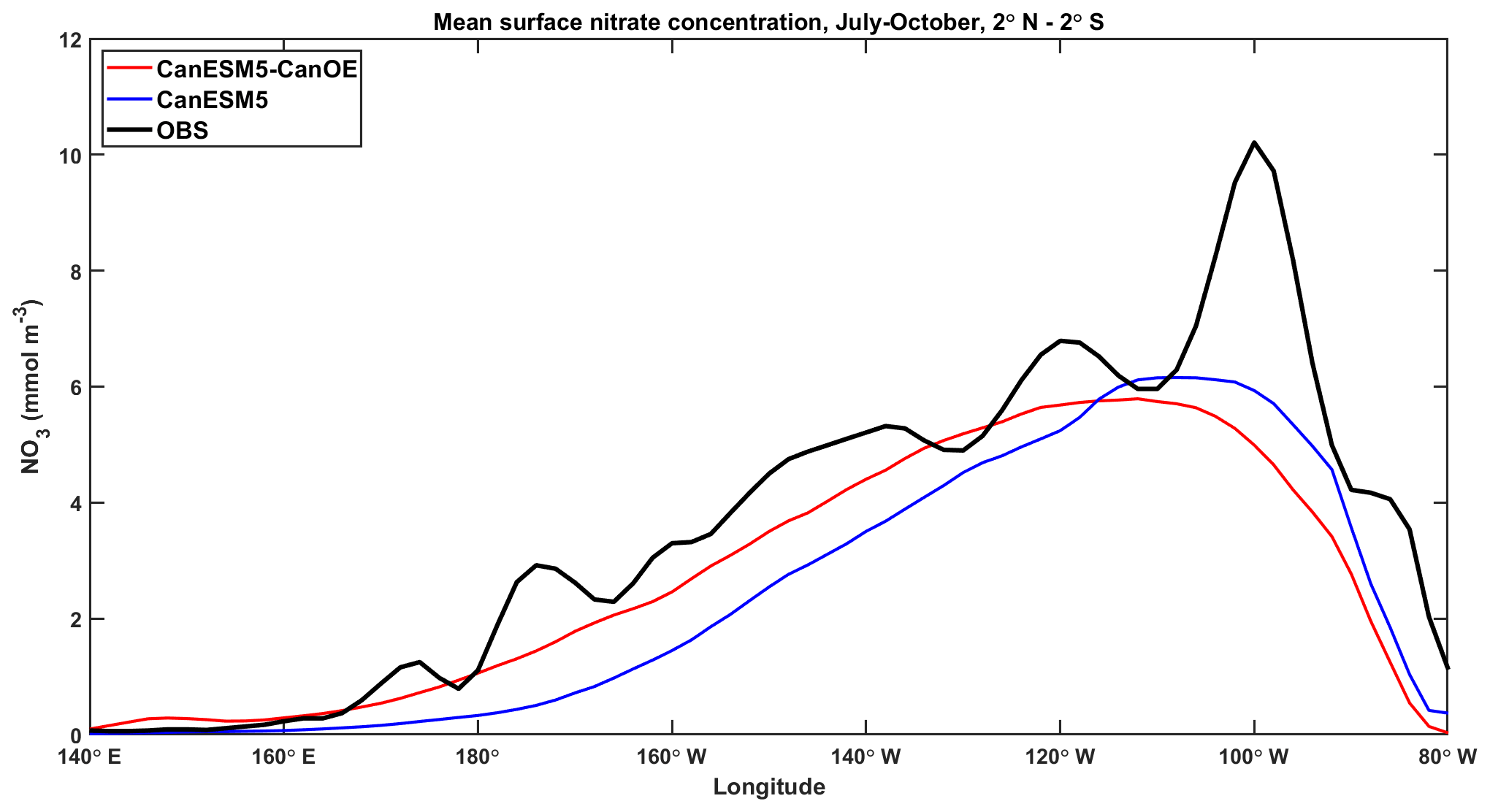
Figure 15Surface nitrate (NO3) concentrations along the Pacific Equator (mean from 2∘ S–2∘ N) during the upwelling season (June–October) for CanESM5-CanOE (red), CanESM5 (blue), and WOA2018 observations (black).
3.4 Plankton biomass, detritus, and particle flux
The relative abundance of the four plankton groups is shown in Fig. 16 for a range of ocean regions. Both CanESM models mostly compare favourably with observation-based estimates of phytoplankton biomass, except in the tropics where CanESM5-CanOE has very high biomass. Both CanESM models have low phytoplankton biomass in the North Atlantic. In the North Pacific and the Southern Ocean, CanESM5-CanOE reproduces the observation-based estimates well and CanESM5 slightly less well. The general pattern is that large and small phytoplankton have similar abundance and are substantially more abundant than zooplankton.
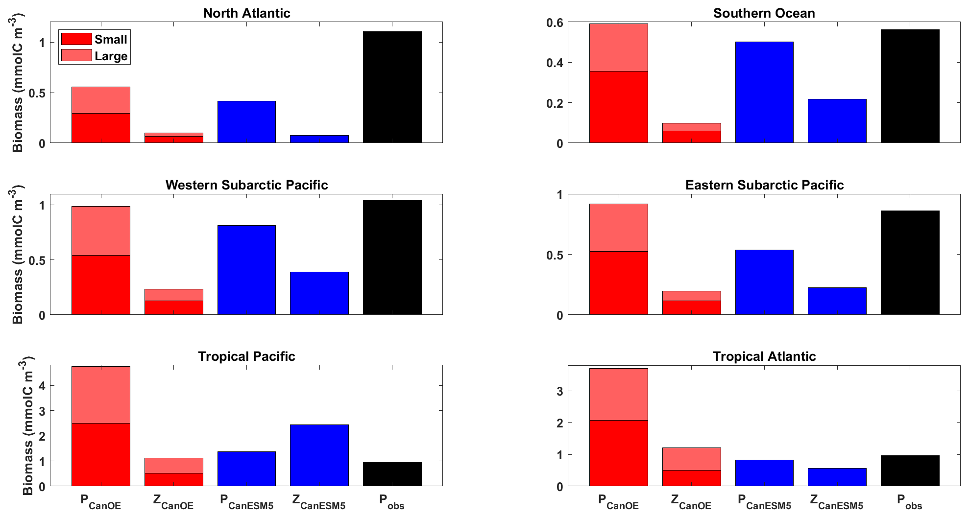
Figure 16Annual mean surface ocean concentration of large and small phytoplankton and zooplankton in CanESM5-CanOE (red) and of phytoplankton and zooplankton in CanESM5 (blue) for the representative ocean regions shown in Fig. 14. Observational estimates (black) are for phytoplankton biomass calculated from satellite ocean colour estimates of surface chlorophyll (SeaWiFS/MODIS; Tesdal et al. 2016), assuming a carbon-to-chlorophyll ratio of 50 g g−1. Region definitions are given in Table S5 and Fig. S5.
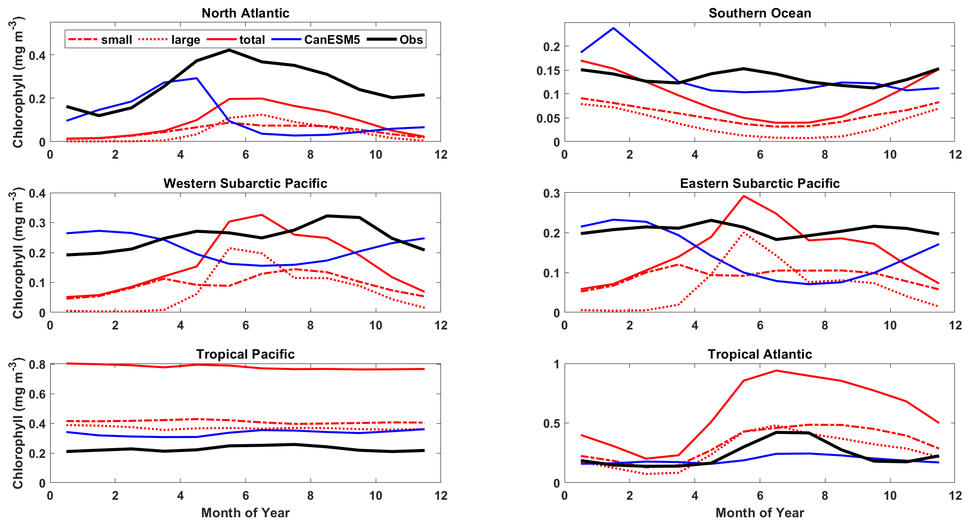
Figure 17Mean annual cycle of surface chlorophyll for the representative ocean regions shown in Figs. 14 and 16. CanESM5-CanOE large and small phytoplankton concentrations are shown separately and combined (red) along with CanESM5 (blue) and observational estimates (black). Region definitions are shown in Table S5 and Fig. S5.

Figure 18Climatological surface particulate organic carbon (POC) vs. chlorophyll for CanESM5-CanOE (red) and observations (black). Data are for all ocean grid points (2×2∘ uniform global grid) for all months of the year where observational data are available. Model POC is offset 17 mg m−3 for illustrative purposes. Chlorophyll concentrations >1 mg m−3 are excluded as they largely represent coastal areas poorly resolved by coarse-resolution global ocean models.
Part of the rationale for multiple food chains is that they better represent the way that actual plankton communities adapt to different physical ocean regimes and therefore are better able to simulate distinct ocean regions with a single parameter set (e.g. Chisholm, 1992; Armstrong, 1994; Landry et al., 1997; Friedrichs et al., 2007). The expectation is that small phytoplankton will be more temporally stable and large phytoplankton will fluctuate more strongly between high and low abundances. The mean annual cycles of surface chlorophyll largely conform to this pattern; e.g. in the North Atlantic and the western subarctic Pacific, large phytoplankton are dominant in summer and much more variable over the seasons (Fig. 17). Compared to observations, CanESM5 models underestimate the amplitude of the seasonal cycle in the North Atlantic and overestimate it in the North Pacific. CanESM5 shows a stronger and earlier North Atlantic spring bloom compared to CanESM5-CanOE; the observations are in between the two in terms of timing, and both models underestimate the amplitude (Fig. 17). In the tropics, the seasonal cycle is weak. CanESM5-CanOE in the tropical Atlantic shows the expected seasonal cycle but not the expected dominance of large phytoplankton in summer. CanESM5-CanOE generally overestimates the total near-surface chlorophyll in both the tropical Pacific and the tropical Atlantic.
Zooplankton biomass (especially microzooplankton) is also somewhat difficult to test against observations, but our model concentrations appear to be biased low. Stock et al. (2014) estimated depth-integrated biomass of phytoplankton, mesozooplankton, and microzooplankton for a range of oceanic locations in which intensive field campaigns have occurred (estimates of microzooplankton biomass are relatively sparse). They found that in most locations phytoplankton and (combined) zooplankton biomass are of comparable magnitude, whereas in CanESM5-CanOE zooplankton biomass is consistently lower (Fig. 16). The global integral biomass of mesozooplankton is about an order of magnitude less than the 0.19 PgC estimated by Moriarty and O'Brien (2013). The CanESM5 total of 0.14 Pg is relatively close to the Moriarty estimate but implicitly includes microzooplankton.
Surface chlorophyll and POC for CanESM5-CanOE and for ocean colour observational data are shown in Fig. 18 (POC in the model is the sum of phytoplankton, microzooplankton, and detrital carbon). The observations have a lower limit for POC that is not present in the model (∼ 17 mgC m−3), which is unsurprising given the processes neglected in the model; i.e. in regions of very low chlorophyll, there is still substantial dissolved organic carbon, bacteria that consume it, and microzooplankton that consume the bacteria and produce particulate detritus. The observational data show a fairly linear relationship at low concentrations, but with a curvature that implies a greater phytoplankton fraction in more eutrophic environments (see Chisholm, 1992). The model, by contrast, shows a fairly linear relationship over the whole range of concentrations. In other words, the phytoplankton share of POC is higher and more constant in the model than in the observations. The living biomass (phytoplankton and microzooplankton) fraction of total POC in CanOE is generally in excess of 50 % (not shown), which is implausible for a real-world oceanic microbial community (e.g. Christian and Karl, 1994) but consistent with the relatively low rates of export from the euphotic zone.
Export production for a range of CMIP6 models is shown in Fig. 19a. CanESM5-CanOE is at the low end of the range. Observations are not shown because the range of observational estimates covers the entire range of model estimates (e.g. Siegel et al., 2016). Note also that CanESM5 export is quite a bit lower than in CanESM2, which is relatively high for CMIP5 models (not shown). The difference between CanESM2 and CanESM5 is attributable primarily to different circulation, although the different initialization fields for nitrate might also play a small role. The lower rate in CanESM5-CanOE is consistent with the above results regarding plankton community structure (e.g. the concentration of detritus is generally low compared to living biomass), as well as the lower sinking rate for small detritus. The latitudinal distribution of export is shown in Fig. 19b. CanESM5 shows very high export in the midlatitudes of the Southern Ocean, similar to CanESM2 (not shown). Both CanESM5 and CanESM5-CanOE show latitudinal patterns consistent with the range of other CMIP6 models. CanESM5 has slightly greater export in the equatorial zone; in both CanESM5 and CanESM5-CanOE, the equatorial enrichment attenuates very rapidly with latitude and the rates are low in the subtropics.

Figure 19(a) Global total export production (epc100) in PgC yr−1 (b) and zonal mean export production in molC m−2 yr−1 according to selected CMIP6 models (mean for 1985–2014 of historical experiment). The thick red line represents CanESM5-CanOE, thick blue line CanESM5, thin grey lines individual CMIP6 models, and thick grey line the model ensemble mean (excluding CanESM5 and CanESM5-CanOE).
3.5 Historical trends
Cumulative ocean uptake of CO2 is shown in Fig. 20 for the historical experiment (1850–2014). CanESM models are biased low relative to observation based estimates (∼ 145 PgC; see Friedlingstein et al., 2020) and the MEM (144 PgC, Fig. 20) but fall well within the spread of CMIP6 models. Some of the difference may be attributable to differences in the way cumulative uptake is calculated in models vs. observations (Bronselaer et al., 2017), although this should apply to other CMIP6 models as well. CanESM5-CanOE has lower cumulative uptake than CanESM5 by ∼ 10 PgC. As the models were not fully equilibrated when the historical run was launched, this difference does not necessarily arise from the biogeochemical model structure; part of the difference can be attributed to differences in the spinup (see Séférian et al., 2016). The drift in the piControl experiment over the 165 years from the branching off of the historical experiment is −10.0 PgC in CanESM5-CanOE and −5.1 PgC in CanESM5 (see Table S6 in the Supplement), so drift accounts for about half (48 %) of the difference in net ocean CO2 uptake. The spatial distribution of anthropogenic DIC is very similar between CanESM5 and CanESM5-CanOE (Fig. S7 in the Supplement). CanESM5 and CanESM5-CanOE show a high bias in near-surface DIC relative to alkalinity (a measure of the ocean's capacity to absorb CO2) in the midlatitudes of both hemispheres (Fig. S8 in the Supplement), which may in part explain the weak uptake of CO2.
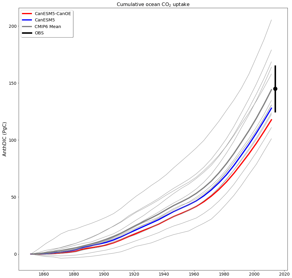
Figure 20Cumulative ocean uptake of carbon dioxide (CO2) as anthropogenic dissolved inorganic carbon (AnthDIC) in PgC over the course of the historical experiment (1850–2014). Data are shown as successive 5-year means. CMIP6 mean (thick grey line) indicates ensemble mean for CMIP6 models (thin grey lines) excluding CanESM5 (blue) and CanESM5-CanOE (red). An observation-based estimate of 145±20 PgC (Friedlingstein et al., 2020) is shown for a nominal year (2014) (black).
The long-term trend in global total export production is shown in Fig. 21. The model values must be normalized in order to compare trends, since the differences among means are large compared to the changes over the historical period (Fig. 19). Such trends are difficult or impossible to meaningfully constrain with observations, but the general expectation has been that export will decline somewhat due to increasing stratification (e.g. Steinacher et al., 2010). CanESM5 shows a greater decline than most other CMIP6 models, while CanESM5-CanOE is more similar to non-CanESM models. The change in CanESM5 is geographically widespread and not concentrated in a specific region or regions: export is maximal in the tropics and the northern and southern midlatitudes (Fig. 19b) and declines over the historical period in all of these regions (Fig. S9 in the Supplement). In CanESM5-CanOE, export declines in the same regions, but the magnitude of the change is smaller, and in the Southern Ocean increases and decreases in different latitude bands largely offset each other.
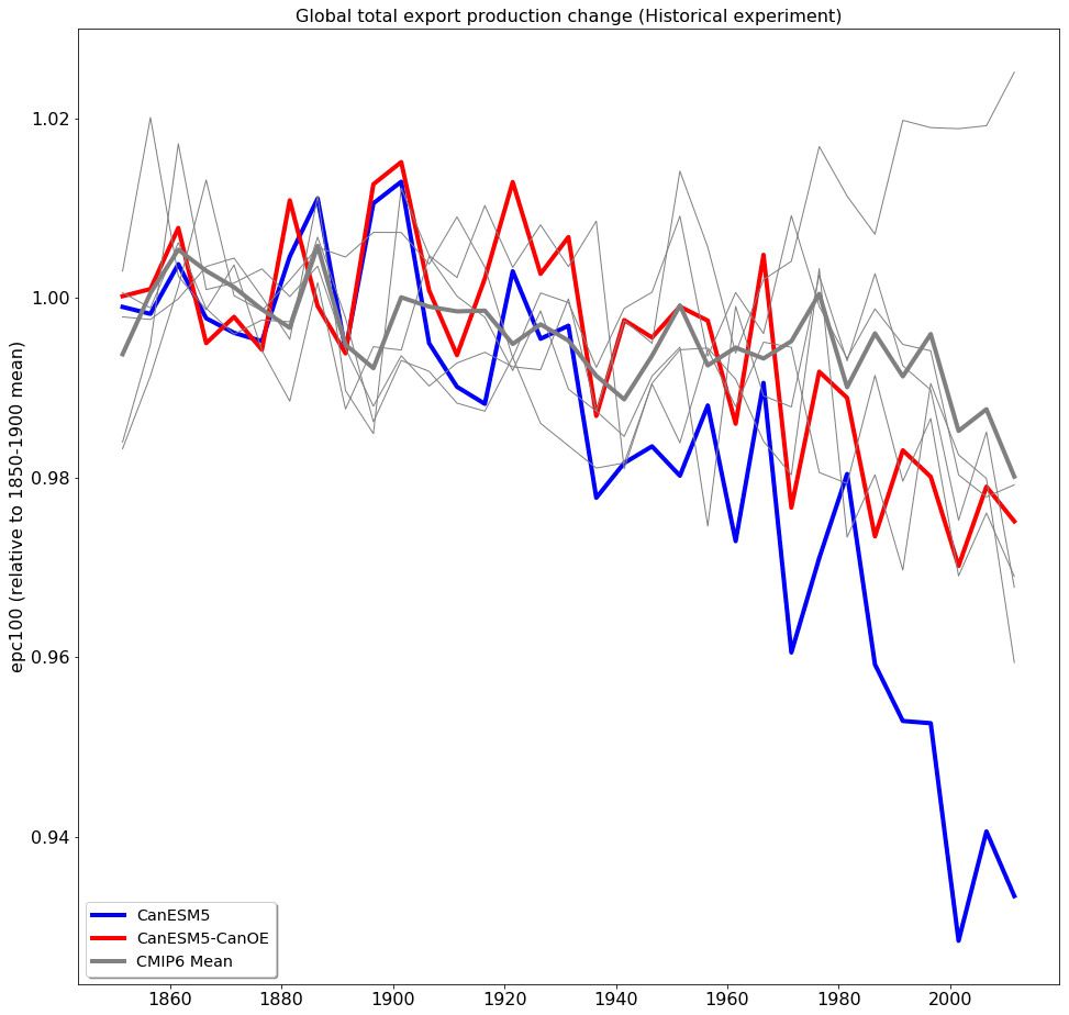
Figure 21Change in export production (epc100) over the course of the historical experiment (1850–2014), normalized to the 1850–1900 mean. Data are shown as successive 5-year means. The thick red line represents CanESM5-CanOE, thick blue line CanESM5, thin grey lines other CMIP6 models, and thick grey line the ensemble mean of non-CanESM models.
The trend in the volume of ocean water with O2 concentration less than 6 or 60 mmol m−3 is shown in Fig. 22. Again, the totals are normalized to a value close to the preindustrial, as the differences among models are large (Fig. 5). For the volume with <60 mmol m−3, CanESM models show relatively little change; in CanESM5, the volume actually declines slightly, while in CanESM5-CanOE it increases, but the total change is <1 % in each case. As with the baseline volumes, the range among models is large, with one model showing an increase approaching 10 % of the total volume estimated for WOA2018 (Figs. 5b and 22b). For the volume with <6 mmol m−3 (Fig. 22a), CanESM models are among the most stable over time. In CanESM5, the volume again declines, although this is within the range of internal variability. Again, some models show fairly large excursions, but in this case none show a strong secular trend over the last half century.
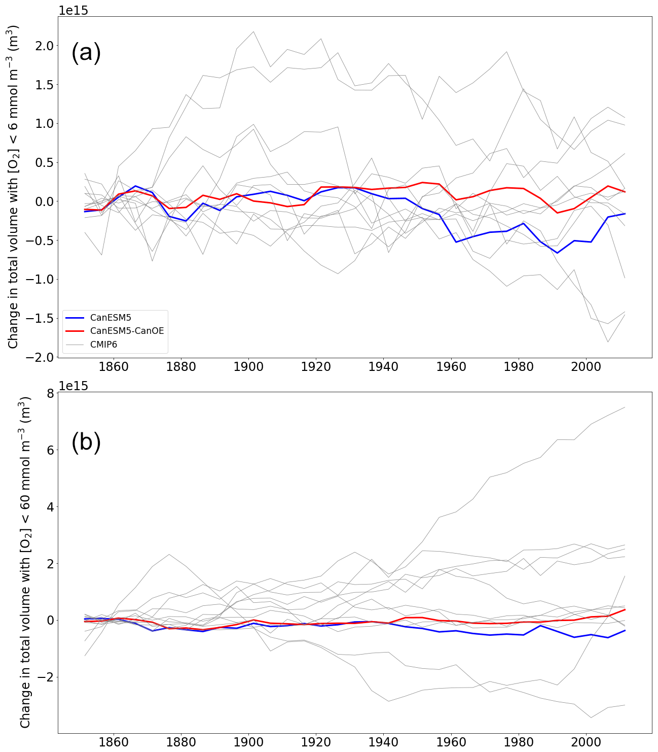
Figure 22(a) Change in total ocean volume with oxygen (O2) concentration less than (a) 6 mmol m−3 and (b) 60 mmol m−3 over the course of the historical experiment (1850–2014), normalized to the 1850–1870 mean. Data are shown as successive 5-year means. The thick red line represents CanESM5-CanOE, thick blue line CanESM5, and thin grey lines other CMIP6 models.
CanESM5 and CanESM5-CanOE are new coupled ocean–atmosphere climate models with prognostic ocean biogeochemistry. The two have the same physical climate (in experiments with specified atmospheric CO2) and differ only in their ocean biogeochemistry components. CanESM5-CanOE has a much more complex biogeochemistry model including a prognostic iron cycle. We have presented results that assess how these two models simulate the overall distribution of major tracers like DIC, alkalinity, nitrate, and oxygen, as well as analyses of the interaction of the iron and nitrogen cycles, plankton community structure, export of organic matter from the euphotic zone, and historical trends over 1850–2014.
The overall distribution of major tracers indicates that both models do a reasonable job of simulating both biogeochemical (e.g. export and remineralization of organic matter) and physical (e.g. deep and intermediate ocean ventilation) processes. The volume of ocean with oxygen concentration below 6 or 60 µM compares favourably with other CMIP6 models (Fig. 5) and is among the most stable over historical time (Fig. 22). CanESM5-CanOE has a substantially lower volume of water with [O2]<6 µM than CanESM5 and much closer to observation-based estimates (Fig. 5). Both models are biased slightly low in terms of historical uptake of anthropogenic CO2, which may indicate weak Southern Ocean upwelling or too-shallow remineralization of DIC or both (Fig. 20). The spatial distribution of anthropogenic DIC is very similar between the two models (Fig. S7 in the Supplement), which is expected as it is mainly a function of the physical ocean model circulation. However, CanESM5 has higher concentrations in the main areas of accumulation, particularly the North Atlantic and the Southern Ocean. This probably indicates more efficient removal and export of “natural” DIC by the plankton, particularly in the Southern Ocean upwelling zone (Fig. 19), and deeper average remineralization, with the caveat that the preindustrial control simulations had different degrees of equilibration when the historical experiment was launched (see Séférian et al., 2016, Table S6 in the Supplement).
Analyses of phytoplankton and zooplankton biomass concentrations show that CanESM5 and CanESM5-CanOE compare somewhat favourably with available observational data but do have distinct biases. In particular, both zooplankton biomass and detrital organic matter concentration tend to be very low in CanESM5-CanOE; the total biomass of the plankton community and the standing crop of particulate organic matter are dominated by phytoplankton (e.g. Fig. 17). Regional biases differ between the two models, with CanESM5-CanOE showing excessively large phytoplankton biomass in the tropics. We note, however, that the seasonal cycle of equatorial upwelling and the formation of the equatorial Pacific HNLC are reproduced rather well by our models (e.g. Figs. 11, 15, and S6), and that CanESM5-CanOE is the first CanESM model to have genuinely simulated this as an emergent property (see Sect. 3.3). In CanESM5-CanOE, decoupling of large and small phytoplankton populations associated with seasonal upwelling or convection (see below) is observed in some regions but not others.
Global export production is biased low, particularly in CanESM5-CanOE. This is due in part to the biogeochemical model and in part to ocean circulation. CanESM5 has the same ocean biology as CanESM2 but a different physical ocean model, and global ocean export production is substantially lower in CanESM5. It is lower still in CanESM5-CanOE (Fig. 19). We note that CanESM5 performs better than CanESM2 on most metrics of physical ocean model evaluation (Swart et al., 2019a) and shows a more realistic distribution of major tracers like DIC (Fig. 8). While the range of observation-based estimates of global ocean export production is large and encompasses the full range of CMIP5 and CMIP6 models, the change between CanESM2 and CanESM5 is large. Changes in the physical ocean are not entirely independent of the biogeochemistry model even when the latter is ostensibly identical. In CanESM2 and CanESM5, iron limitation is specified as a spatially static “mask” based on the observed distribution of surface nitrate, and it is possible that in these two models ocean upwelling occurs in different places relative to the specified boundary of the region of Southern Ocean iron imitation (Fig. 3 of Zahariev et al., 2008). It is also possible that the lower export production in CanESM5-CanOE is due to low iron supply to the surface waters of the Southern Ocean, but comparisons with available observations do not suggest that this is the case. Several biases are common to CanESM5 and CanESM5-CanOE that relate to Southern Ocean upwelling (high Southern Ocean surface nitrate concentration, low export production, weak anthropogenic CO2 uptake) and so are probably more attributable to the physical ocean model than to the Fe submodel. The difference between CanESM2 and CanESM5 bears this out.
The development of CanOE was undertaken in response to some of the most severe limitations of CanESM2. Many of the additional features that CanOE introduces were already in the models published by other centres even in CMIP5. In addition to CMOC (Zahariev et al., 2008), previous models developed by members of our group include Denman and Peña (1999; 2002), Christian et al. (2002a, b), Christian (2005), and Denman et al. (2006). Christian et al. (2002a) had a prognostic Fe cycle and multiple phytoplankton and zooplankton species but had fixed elemental ratios. Christian (2005) incorporated a cellular-regulation model but only for a single species and without Fe limitation. Christian (2005) had prognostic chlorophyll, whereas Denman and Peña (1999; 2002) and Christian et al. (2002a) used an irradiance-dependent diagnostic formulation. Christian et al. (2002a) used multiplicative (Franks et al., 1986) grazing, which creates stability in predator–prey interactions but severely limits phytoplankton biomass accumulation under nutrient-replete conditions.
One of the most important lessons from Christian et al. (2002a, b) was that when a fixed ratio is employed, sensitivity to this parameter is extreme. Because Fe cell quotas are far more variable than N, P, or Si quotas, treating this parameter as constant results in the specified value influencing the overall solution far more than any other parameter. CanESM5-CanOE largely succeeded in creating a prognostic Fe–N limitation model that produces HNLC conditions in the expected regions (Figs. 10, 11, 14, 15, S6), although surface nitrate concentration is low relative to observation-based estimates in some cases. External Fe sources and scavenging parameterizations will be revisited and refined in future versions. In CanESM5-CanOE, the scavenging model is very simple, with distinct regimes for concentrations greater or less than 0.6 nM; scavenging rates are very high above this threshold which causes deep-water concentrations to converge on this value. The generally nutrient-like profile suggest that in CanOE the scavenging rate is quite low for concentrations below 0.6 nM (Fig. 13; see also Fig. S10h in the Supplement). We note that the aeolian mineral dust deposition field employed here is derived from the CanESM atmosphere model; these processes are not presently interactive but could be made so in the future.
A particular issue with CanESM2 was that extremely high concentrations of nitrate occurred under the EBC upwelling regions. This error resulted from spreading denitrification out over the ocean basin so that introduction of new fixed N from N2 fixation would balance denitrification losses within each vertical column, whereas in the real world denitrification is highly localized in the low oxygen environments under the EBCs. CanESM2 did not include oxygen, but CanESM5 incorporates oxygen as a “downstream” tracer that does not feed back on other biogeochemical processes. The incorporation of a more process-based denitrification parameterization in CanESM5-CanOE is independent of the many other processes that are present in CanESM5-CanOE but not in CanESM5: a CMOC-like model with prognostic denitrification is clearly an option. We chose not to include explicit, oxygen-dependent denitrification in CanESM5 because we wanted to maintain a CMOC-based model as close to the CanESM2 version as possible, and because oxygen would not then be a downstream tracer that does not affect other processes.
Plankton community structure in CanESM5-CanOE is somewhat biased toward high concentrations of phytoplankton, low concentrations of zooplankton and detritus, and low export (Sect. 3.4). In the development phase, a fair number of experiments were conducted with various values of the grazing rates and detritus sinking speeds. A wide range of values of these parameters was tested, with no resulting improvement in the overall results. Possibly the detrital remineralization rates are too high, although primary production is also on the low end of the CMIP6 range (not shown) and would probably decline further if these rates were decreased. The model was designed around the Armstrong (1994) hypothesis of “supplementation” vs. “replacement”; i.e. small phytoplankton and their grazers do not become much more abundant in more nutrient-rich environments but rather stay at about the same level and are joined by larger species that are absent in more oligotrophic conditions (see also Chisholm, 1992; Landry et al., 1997; Friedrichs et al., 2007). The results presented here suggest that this was partially achieved, but further improvement is possible (Fig. 17).
As to whether the gains in skill with CanESM5-CanOE justify the extra computational cost, Taylor diagrams (Figs. 4, 8, 9, and Fig. S4 in the Supplement) show a modest but consistent gain in skill at simulating the major biogeochemical species (O2, DIC, alkalinity) across variables and depths, especially for alkalinity at middle depths (Fig. S4 in the Supplement), for which CanESM5 displays the least skill relative to other fields or depths. Other processes that are highly parameterized in CanESM5, such as calcification and CaCO3 dissolution, were not addressed in detail in this paper but are an important factor in determining the subsurface distribution of alkalinity. Again, we emphasize that we are simulating as an emergent property of a process-based model something that is parameterized in CanESM5 (as previously noted for surface nitrate concentration in HNLC regions), and doing at least as well in terms of model skill. As a general rule, the potential for improving skill and achieving better results in novel environments (e.g. topographically complex regional domains like the Arctic Ocean and the boreal marginal seas) is expected to be greater in less parameterized, more mechanistic models (e.g. Friedrichs et al., 2007; Tesdal et al., 2016). Inclusion of a prognostic iron cycle and C/N/Fe stoichiometry also open up additional applications and scientific investigations that are not possible with CMOC.
An updated version of CanESM5 with prognostic denitrification is clearly possible. However, for the reasons discussed above, a prognostic Fe cycle with a fixed phytoplankton remains problematic, and the model would still have a single detritus sinking speed and remineralization length scale. We are also developing CanOE for regional downscaling applications (Hayashida, 2018; Holdsworth et al., 2021). The regional domains have complex topography and prominent continental shelf and slope, and the single remineralization length scale in CMOC may not be well suited to such an environment. The number of tracers in CanOE is not particularly large compared with other CMIP6 models. We expect to further refine CanOE and its parameterizations, evaluate it against new and emerging ocean data sets (e.g. GEOTRACES, biogeochemical Argo), and incrementally improve CMOC (which we will maintain for a wide suite of physical climate experiments for which ocean biogeochemistry is not central to the purpose). For CMIP6, we chose to keep CMOC as close to the CanESM2 version as possible. This strategy allows us to quantify how much of the improvement in model skill is due to the physical circulation, as is illustrated by greater skill with respect to DIC (Fig. 8) and alkalinity (Fig. S4 in the Supplement), particularly at intermediate depths (400–900 m). The CanESM terrestrial carbon model is also undergoing important new developments (e.g. Asaadi and Arora, 2021) and we expect CanESM to continue to offer a credible contribution to global carbon cycle studies, as well as advance regional downscaling and impact science.
The full CanESM5 source code is publicly available at https://gitlab.com/cccma/canesm (last access: 19 May 2022); within this tree, the ocean biogeochemistry code can be found at https://gitlab.com/cccma/cannemo/-/tree/v5.0.3/nemo/CONFIG/CCC_CANCPL_ORCA1_LIM_CMOC (last access: 19 May 2022) or https://gitlab.com/cccma/cannemo/-/tree/v5.0.3/nemo/CONFIG/CCC_CANCPL_ORCA1_LIM_CANOE (last access: 19 May 2022). The version of the code which can be used to produce all the simulations submitted to CMIP6, and described in this paper, is tagged as v5.0.3 and has the associated DOI: https://doi.org/10.5281/zenodo.3251114 (Swart et al., 2019b).
All simulations conducted for CMIP6, including those described in this paper, are publicly available via the Earth System Grid Federation (source_id = CanESM5 or CanESM5-CanOE). All observational data and other CMIP6 model data used are publicly available.
The supplement related to this article is available online at: https://doi.org/10.5194/gmd-15-4393-2022-supplement.
JRC, KLD, NS, and NCS were responsible for the formulation of the overall research goals and aims. JRC, HH, AMH, WGL, OGJR, AES, and NCS were responsible for implementation and testing of the model code. JRC, WGL, OGJR, AES, and NCS carried out the experiments. JRC, HH, AMH, AES, NS, and NCS were responsible for creation of the published work.
The contact author has declared that neither they nor their co-authors have any competing interests.
CanESM has been customized to run on the ECCC high-performance computer,
and a significant fraction of the software infrastructure used to run the
model is specific to the individual machines and architecture. While we
publicly provide the code, we cannot provide any support for migrating the
model to different machines or architectures.
Publisher’s note: Copernicus Publications remains neutral with regard to jurisdictional claims in published maps and institutional affiliations.
This work was made possible by the combined efforts of the CCCMa model development team and computing support team. We thank all of the data contributors to and developers of the observational data products, the NASA Ocean Color team, and all of the CMIP6 data contributors. The Python packages mocsy by Jim Orr and SkillMetrics by Peter Rochford were invaluable tools in the analysis. John Dunne, William Merryfield, Anh Pham, Andrew Ross, and several anonymous reviewers made useful comments on earlier drafts. Fiona Davidson helped with figure preparation. This paper is dedicated to the memory of Fouad Majaess, who supported CCCMa supercomputer users for many years and passed away suddenly in 2020.
This paper was edited by Riccardo Farneti and reviewed by Anh Pham, John Dunne, and two anonymous referees.
Arguez, A. and Vose, R.: The Definition of the Standard WMO Climate Normal The Key to Deriving Alternative Climate Normals, B. Am. Meteorol. Soc., 92, 699–704, https://doi.org/10.1175/2010BAMS2955.1, 2011.
Armstrong, R.: Grazing limitation and nutrient limitation in marine ecosystems - steady-state solutions of an ecosystem model with multiple food-chains, Limnol. Oceanogr., 39, 597–608, 1994.
Arora, V., Scinocca, J., Boer, G., Christian, J., Denman, K., Flato, G., Kharin, V., Lee, W., and Merryfield, W.: Carbon emission limits required to satisfy future representative concentration pathways of greenhouse gases, Geophys. Res. Lett., 38, L05805, https://doi.org/10.1029/2010GL046270, 2011.
Arora, V. K., Katavouta, A., Williams, R. G., Jones, C. D., Brovkin, V., Friedlingstein, P., Schwinger, J., Bopp, L., Boucher, O., Cadule, P., Chamberlain, M. A., Christian, J. R., Delire, C., Fisher, R. A., Hajima, T., Ilyina, T., Joetzjer, E., Kawamiya, M., Koven, C. D., Krasting, J. P., Law, R. M., Lawrence, D. M., Lenton, A., Lindsay, K., Pongratz, J., Raddatz, T., Séférian, R., Tachiiri, K., Tjiputra, J. F., Wiltshire, A., Wu, T., and Ziehn, T.: Carbon–concentration and carbon–climate feedbacks in CMIP6 models and their comparison to CMIP5 models, Biogeosciences, 17, 4173–4222, https://doi.org/10.5194/bg-17-4173-2020, 2020.
Asaadi, A. and Arora, V. K.: Implementation of nitrogen cycle in the CLASSIC land model, Biogeosciences, 18, 669–706, https://doi.org/10.5194/bg-18-669-2021, 2021.
Aumont, O., Ethé, C., Tagliabue, A., Bopp, L., and Gehlen, M.: PISCES-v2: an ocean biogeochemical model for carbon and ecosystem studies, Geosci. Model Dev., 8, 2465–2513, https://doi.org/10.5194/gmd-8-2465-2015, 2015.
Babbin, A., Keil, R., Devol, A., and Ward, B.: Organic Matter Stoichiometry, Flux, and Oxygen Control Nitrogen Loss in the Ocean, Science, 344, 406–408, https://doi.org/10.1126/science.1248364, 2014.
Bronselaer, B., Winton, M., Russell, J., Sabine, C., and Khatiwala, S.: Agreement of CMIP5 Simulated and Observed Ocean Anthropogenic CO2 Uptake, Geophys. Res. Lett., 44, 12298–12305, https://doi.org/10.1002/2017GL074435, 2017.
Chisholm, S. W.: Phytoplankton size, in: Primary productivity and biogeochemical cycles in the sea, edited by: Falkowski, P. G. and Woodhead A. D., Plenum, New York, 213–237, https://doi.org/10.1007/978-1-4899-0762-2, 1992.
Christian, J.: Biogeochemical cycling in the oligotrophic ocean: Redfield and non-Redfield models, Limnol. Oceanogr., 50, 646–657, 2005.
Christian, J. and Karl, D.: Microbial community structure at the United States Joint Global Ocean Flux Study Station ALOHA – inverse methods for estimating biochemical indicator ratios, J. Geophys. Res.-Oceans, 99, 14269–14276, https://doi.org/10.1029/94JC00681, 1994.
Christian, J., Arora, V., Boer, G., Curry, C., Zahariev, K., Denman, K., Flato, G., Lee, W., Merryfield, W., Roulet, N., and Scinocca, J.: The global carbon cycle in the Canadian Earth system model (CanESM1): Preindustrial control simulation, J. Geophys. Res.-Biogeosciences, 115, G03014, https://doi.org/10.1029/2008JG000920, 2010.
Christian, J. R., Verschell, M. A., Murtugudde, R., Busalacchi, A. J., and McClain, C. R.: Biogeochemical modelling of the tropical Pacific Ocean, I: Seasonal and interannual variability, Deep-Sea Res. Pt. II, 49, 509–543, 2002a.
Christian, J. R., Verschell, M. A., Murtugudde, R., Busalacchi, A. J., and McClain, C. R.: Biogeochemical modelling of the tropical Pacific Ocean, II: Iron biogeochemistry, Deep-Sea Res. Pt. II, 49, 545–565, https://doi.org/10.1016/s0967-0645(01)00111-4, 2002b.
Denman, K. and Pena, M.: A coupled 1-D biological/physical model of the northeast subarctic Pacific Ocean with iron limitation, Deep-Sea Res. Pt. II, 46, 2877–2908, https://doi.org/10.1016/S0967-0645(99)00087-9, 1999.
Denman, K. and Pena, M.: The response of two coupled one-dimensional mixed layer/planktonic ecosystem models to climate change in the NE subarctic Pacific Ocean, Deep-Sea Res. Pt. II, 49, 5739–5757, https://doi.org/10.1016/S0967-0645(02)00212-6, 2002.
Denman, K., Voelker, C., Pena, M., and Rivkin, R.: Modelling the ecosystem response to iron fertilization in the subarctic NE Pacific: The influence of grazing, and Si and N cycling on CO2 drawdown, Deep-Sea Res. Pt. II, 53, 2327–2352, https://doi.org/10.1016/j.dsr2.2006.05.026, 2006.
Devol, A. H.: Denitrification including anammox, in: Nitrogen in the Marine Environment, 2nd edition, edited by: Capone, D. G., Bronk, D. A., Mulholland, M.R., and Carpenter, E. J., Elsevier, Amsterdam, 263–301, https://doi.org/10.1016/B978-0-12-372522-6.X0001-1, 2008.
Dickson, A. G., Sabine, C. L., and Christian, J. R.: Guide to best practices for ocean CO2 measurements, PICES Special Publication 3, 191 p., ISBN 1897176074, 2007.
Elser, J. and Urabe, J.: The stoichiometry of consumer-driven nutrient recycling: Theory, observations, and consequences, Ecology, 80, 735–751, https://doi.org/10.1890/0012-9658(1999)080[0735:TSOCDN]2.0.CO;2, 1999.
Franks, P., Wroblewski, J., and Flierl, G.: Behavior of a simple plankton model with food-level acclimation by herbivores, Mar. Biol., 91, 121–129, https://doi.org/10.1007/BF00397577, 1986.
Friedlingstein, P., O'Sullivan, M., Jones, M. W., Andrew, R. M., Hauck, J., Olsen, A., Peters, G. P., Peters, W., Pongratz, J., Sitch, S., Le Quéré, C., Canadell, J. G., Ciais, P., Jackson, R. B., Alin, S., Aragão, L. E. O. C., Arneth, A., Arora, V., Bates, N. R., Becker, M., Benoit-Cattin, A., Bittig, H. C., Bopp, L., Bultan, S., Chandra, N., Chevallier, F., Chini, L. P., Evans, W., Florentie, L., Forster, P. M., Gasser, T., Gehlen, M., Gilfillan, D., Gkritzalis, T., Gregor, L., Gruber, N., Harris, I., Hartung, K., Haverd, V., Houghton, R. A., Ilyina, T., Jain, A. K., Joetzjer, E., Kadono, K., Kato, E., Kitidis, V., Korsbakken, J. I., Landschützer, P., Lefèvre, N., Lenton, A., Lienert, S., Liu, Z., Lombardozzi, D., Marland, G., Metzl, N., Munro, D. R., Nabel, J. E. M. S., Nakaoka, S.-I., Niwa, Y., O'Brien, K., Ono, T., Palmer, P. I., Pierrot, D., Poulter, B., Resplandy, L., Robertson, E., Rödenbeck, C., Schwinger, J., Séférian, R., Skjelvan, I., Smith, A. J. P., Sutton, A. J., Tanhua, T., Tans, P. P., Tian, H., Tilbrook, B., van der Werf, G., Vuichard, N., Walker, A. P., Wanninkhof, R., Watson, A. J., Willis, D., Wiltshire, A. J., Yuan, W., Yue, X., and Zaehle, S.: Global Carbon Budget 2020, Earth Syst. Sci. Data, 12, 3269–3340, https://doi.org/10.5194/essd-12-3269-2020, 2020.
Friedrichs, M., Dusenberry, J., Anderson, L., Armstrong, R., Chai, F., Christian, J., Doney, S., Dunne, J., Fujii, M., Hood, R., McGillicuddy, D., Moore, J., Schartau, M., Spitz, Y., and Wiggert, J.: Assessment of skill and portability in regional marine biogeochemical models: Role of multiple planktonic groups, J. Geophys. Res.-Oceans, 112, C08001, https://doi.org/10.1029/2006JC003852, 2007.
Garcia, H. E., Weathers, K., Paver, C. R., Smolyar, I., Boyer, T. P., Locarnini, R. A., Zweng, M. M., Mishonov, A. V., Baranova, O. K., Seidov, D., and Reagan, J. R.: World Ocean Atlas 2018, Volume 3: Dissolved Oxygen, Apparent Oxygen Utilization, and Oxygen Saturation. A. Mishonov Technical Ed., NOAA Atlas NESDIS 83 [data set], 38 p., https://www.ncei.noaa.gov/archive/accession/NCEI-WOA18 (last access: 19 May 2022), 2018a.
Garcia, H. E., Weathers, K., Paver, C. R., Smolyar, I., Boyer, T. P., Locarnini, R. A., Zweng, M. M., Mishonov, A. V., Baranova, O. K., Seidov, D. and Reagan, J. R.: World Ocean Atlas 2018, Volume 4: Dissolved Inorganic Nutrients (phosphate, nitrate and nitrate+nitrite, silicate), A. Mishonov Technical Ed., NOAA Atlas NESDIS 84 [data set], 35 p., https://www.ncei.noaa.gov/archive/accession/NCEI-WOA18 (last access: 19 May 2022), 2018b.
Geider, R., MacIntyre, H., and Kana, T.: A dynamic regulatory model of phytoplanktonic acclimation to light, nutrients, and temperature, Limnol. Oceanogr., 43, 679–694, 1998.
Guilyardi, E. and Madec, G.: Performance of the OPA/ARPEGE-T21 global ocean-atmosphere coupled model, Clim. Dynam., 13, 149–165, https://doi.org/10.1007/s003820050157, 1997.
Hayashida, H.: Modelling sea-ice and oceanic dimethylsulfide production and emissions in the Arctic, PhD thesis, University of Victoria, https://hdl.handle.net/1828/10486 (last access: 30 May 2022), 2018.
Holdsworth, A. M., Zhai, L., Lu, Y., and Christian, J. R.: Future changes in oceanography and biogeochemistry along the Canadian Pacific continental margin, Frontiers in Marine Science, 8, 2296–7745, https://doi.org/10.3389/fmars.2021.602991, 2021.
Jetten, M., Wagner, M., Fuerst, J., van Loosdrecht, M., Kuenen, G., and Strous, M.: Microbiology and application of the anaerobic ammonium oxidation (“anammox”) process, Curr. Opin. Biotech., 12, 283–288, https://doi.org/10.1016/S0958-1669(00)00211-1, 2001.
Johnson, K., Elrod, V., Fitzwater, S., Plant, J., Chavez, F., Tanner, S., Gordon, R., Westphal, D., Perry, K., Wu, J., and Karl, D.: Surface ocean-lower atmosphere interactions in the Northeast Pacific Ocean Gyre: Aerosols, iron, and the ecosystem response, Global Biogeochem. Cy., 17, 1063, https://doi.org/10.1029/2002GB002004, 2003.
Johnson, K. S., Gordon, R. M., and Coale, K. H.: What controls dissolved iron concentrations in the world ocean?, Mar. Chem., 57, 137–161, https://doi.org/10.1016/s0304-4203(97)00043-1, 1997.
Key, R. M., Olsen, A., van Heuven, S., Lauvset, S. K., Velo, A., Lin, X., Schirnick, C., Kozyr, A., Tanhua, T., Hoppema, M., Jutterström, S., Steinfeldt, R., Jeansson, E., Ishii, M., Perez, F. F., and Suzuki, T.: Global Ocean Data Analysis Project, Version 2 (GLODAPv2), ORNL/CDIAC-162, NDP-093, Carbon Dioxide Information Analysis Center, Oak Ridge National Laboratory, US Department of Energy, Oak Ridge, Tennessee, https://www.glodap.info/wp-content/uploads/2017/08/NDP_093.pdf (last access: 19 May 2022), 2015.
Lambert, S. and Boer, G.: CMIP1 evaluation and intercomparison of coupled climate models, Clim. Dynam., 17, 83–106, https://doi.org/10.1007/PL00013736, 2001.
Landry, M., Barber, R., Bidigare, R., Chai, F., Coale, K., Dam, H., Lewis, M., Lindley, S., McCarthy, J., Roman, M., Stoecker, D., Verity, P., and White, J.: Iron and grazing constraints on primary production in the central equatorial Pacific: An EqPac synthesis, Limnol. Oceanogr., 42, 405–418, https://doi.org/10.4319/lo.1997.42.3.0405, 1997.
Lauvset, S. K., Key, R. M., Olsen, A., van Heuven, S., Velo, A., Lin, X., Schirnick, C., Kozyr, A., Tanhua, T., Hoppema, M., Jutterström, S., Steinfeldt, R., Jeansson, E., Ishii, M., Perez, F. F., Suzuki, T., and Watelet, S.: A new global interior ocean mapped climatology: the GLODAP version 2, Earth Syst. Sci. Data, 8, 325–340, https://doi.org/10.5194/essd-8-325-2016, 2016.
Li, Y.: Distribution patterns of the elements in the ocean – a synthesis, Geochim. Cosmochim. Ac., 55, 3223–3240, 1991.
Locarnini, R. A., Mishonov, A. V., Antonov, J. I., Boyer, T. P., Garcia, H. E., Baranova, O. K., Zweng, M. M., and Johnson, D. R.: World Ocean Atlas 2009, Volume 1: Temperature, edited by: Levitus, S., NOAA Atlas NESDIS 68 [data set], 184 p., https://www.ncei.noaa.gov/archive/accession/0094866 (last access: 30 May 2022), 2010.
Locarnini, R. A., Mishonov, A. V., Baranova, O. K., Boyer, T. P., Zweng, M. M., Garcia, H. E., Reagan, J. R., Seidov, D., Weathers, K., Paver, C. R., and Smolyar, I.: World Ocean Atlas 2018, Volume 1: Temperature, edited by: Mishonov A., NOAA Atlas NESDIS 81 [data set], 52 p., https://www.ncei.noaa.gov/archive/accession/NCEI-WOA18 (last access: 19 May 2022) 2018.
Loladze, I., Kuang, Y., and Elser, J.: Stoichiometry in producer-grazer systems: Linking energy flow with element cycling, B. Math. Biol., 62, 1137–1162, https://doi.org/10.1006/bulm.2000.0201, 2000.
Lukas, R.: Pacific ocean equatorial currents, in: Encyclopedia of Ocean Sciences, edited by: Steele, J. H., Thorpe, S. A., and Turekian, K. K., Academic, San Diego, 2069–2076, https://doi.org/10.1006/rwos.2001.0354, 2001.
Madec, G. and Imbard, M.: A global ocean mesh to overcome the North Pole singularity, Clim. Dynam., 12, 381–388, https://doi.org/10.1007/s003820050115, 1996.
Moriarty, R. and O'Brien, T. D.: Distribution of mesozooplankton biomass in the global ocean, Earth Syst. Sci. Data, 5, 45–55, https://doi.org/10.5194/essd-5-45-2013, 2013.
Nozaki, Y.: Elemental Distribution, in: Encyclopedia of Ocean Sciences, edited by: Steele, J. H., Thorpe, S. A., and Turekian, K. K., Academic, San Diego, Encyclopedia of Ocean Sciences, 840–845, https://doi.org/10.1006/rwos.2001.0402, 2001.
Orr, J. C., Najjar, R. G., Aumont, O., Bopp, L., Bullister, J. L., Danabasoglu, G., Doney, S. C., Dunne, J. P., Dutay, J.-C., Graven, H., Griffies, S. M., John, J. G., Joos, F., Levin, I., Lindsay, K., Matear, R. J., McKinley, G. A., Mouchet, A., Oschlies, A., Romanou, A., Schlitzer, R., Tagliabue, A., Tanhua, T., and Yool, A.: Biogeochemical protocols and diagnostics for the CMIP6 Ocean Model Intercomparison Project (OMIP), Geosci. Model Dev., 10, 2169–2199, https://doi.org/10.5194/gmd-10-2169-2017, 2017.
Philander, S. G. and Chao, Y.: On the contrast between the seasonal cycles of the equatorial Atlantic and Pacific oceans, J. Phys. Ocean., 21, 1399–1406, 1991.
Raven, J. and Geider, R.: Temperature and algal growth, New Phytologist, 110, 441–461, https://doi.org/10.1111/j.1469-8137.1988.tb00282.x, 1988.
Riche, O. and Christian, J.: Ocean dinitrogen fixation and its potential effects on ocean primary production in Earth system model simulations of anthropogenic warming, Elementa-Science of the Anthropocene, 6, 16, https://doi.org/10.1525/elementa.277, 2018.
Schlitzer, R., Anderson, R., Dodas, E., Lohan, M., Geibere, W., Tagliabue, A., Bowie, A., Jeandel, C., Maldonado, M., Landing, W., Cockwell, D., Abadie, C., Abouchami, W., Achterberg, E., Agather, A., Aguliar-Islas, A., van Aken, H., Andersen, M., Archer, C., Auro, M., de Baar, H., Baars, O., Baker, A., Bakker, K., Basak, C., Baskaran, M., Bates, N., Bauch, D., van Beek, P., Behrens, M., Black, E., Bluhm, K., Bopp, L., Bouman, H., Bowman, K., Bown, J., Boyd, P., Boye, M., Boyle, E., Branellec, P., Bridgestock, L., Brissebrat, G., Browning, T., Bruland, K., Brumsack, H., Brzezinski, M., Buck, C., Buck, K., Buesseler, K., Bull, A., Butler, E., Cai, P., Mor, P., Cardinal, D., Carlson, C., Carrasco, G., Casacuberta, N., Casciotti, K., Castrillejo, M., Chamizo, E., Chance, R., Charette, M., Chaves, J., Cheng, H., Chever, F., Christl, M., Church, T., Closset, I., Colman, A., Conway, T., Cossa, D., Croot, P., Cullen, J., Cutter, G., Daniels, C., Dehairs, F., Deng, F., Dieu, H., Duggan, B., Dulaquais, G., Dumousseaud, C., Echegoyen-Sanz, Y., Edwards, R., Ellwood, M., Fahrbach, E., Fitzsimmons, J., Flegal, A., Fleisher, M., van de Flierdt, T., Frank, M., Friedrich, J., Fripiat, F., Frollje, H., Galer, S., Gamo, T., Ganeshram, R., Garcia-Orellana, J., Garcia-Solsona, E., Gault-Ringold, M., George, E., Gerringa, L., Gilbert, M., Godoy, J., Goldstein, S., Gonzalez, S., Grissom, K., Hammerschmidt, C., Hartman, A., Hassler, C., Hathorne, E., Hatta, M., Hawco, N., Hayes, C., Heimburger, L., Helgoe, J., Heller, M., Henderson, G., Henderson, P., van Heuven, S., Ho, P., Horner, T., Hsieh, Y., Huang, K., Humphreys, M., Isshiki, K., Jacquot, J., Janssen, D., Jenkins, W., John, S., Jones, E., Jones, J., Kadko, D., Kayser, R., Kenna, T., Khondoker, R., Kim, T., Kipp, L., Klar, J., Klunder, M., Kretschmer, S., Kumamoto, Y., Laan, P., Labatut, M., Lacan, F., Lam, P., Lambelet, M., Lamborg, C., Le Moigne, F., Le Roy, E., Lechtenfeld, O., Lee, J., Lherminier, P., Little, S., Lopez-Lora, M., Lu, Y., Masque, P., Mawji, E., Mcclain, C., Measures, C., Mehic, S., Menzel Barraqueta, J., van der Merwe, P., Middag, R., Mieruch, S., Milne, A., Minami, T., Moffett, J., Moncoiffe, G., Moore, W., Morris, P., Morton, P., Nakaguchi, Y., Nakayama, N., Niedermiller, J., Nishioka, J., Nishiuchi, A., Noble, A., Obata, H., Ober, S., Ohnemus, D., van Ooijen, J., O'Sullivan, J., Owens, S., Pahnke, K., Paul, M., Pavia, F., Pena, L., Petersh, B., Planchon, F., Planquette, H., Pradoux, C., Puigcorbe, V., Quay, P., Queroue, F., Radic, A., Rauschenberg, S., Rehkamper, M., Rember, R., Remenyi, T., Resing, J., Rickli, J., Rigaud, S., Rijkenberg, M., Rintoul, S., Robinson, L., Roca-Marti, M., Rodellas, V., Roeske, T., Rolison, J., Rosenberg, M., Roshan, S., van der Loaff, M., Ryabenko, E., Saito, M., Salt, L., Sanial, V., Sarthou, G., Schallenberg, C., Schauer, U., Scher, H., Schlosser, C., Schnetger, B., Scott, P., Sedwick, P., Semiletov, I., Shelley, R., Sherrell, R., Shiller, A., Sigman, D., Singh, S., Slagter, H., Slater, E., Smethie, W., Snaith, H., Sohrin, Y., Sohst, B., Sonke, J., Speich, S., Steinfeldt, R., Stewart, G., Stichel, T., Stirling, C., Stutsman, J., Swarr, G., Swift, J., Thomas, A., Thorne, K., Till, C., Till, R., Townsend, A., Townsend, E., Tuerena, R., Twining, B., Vance, D., Velazquez, S., Venchiarutti, C., Villa-Alfageme, M., Vivancos, S., Voelker, A., Wake, B., Warner, M., Watson, R., van Weerlee, E., Weigand, M., Weinstein, Y., Weiss, D., Wisotzki, A., Woodward, E., Wu, J., Wu, Y., Wuttig, K., Wyatt, N., Xiang, Y., Xie, R., Xue, Z., Yoshikawa, H., Zhang, J., Zhang, P., Zhao, Y., Zheng, L., Zheng, X., Zieringer, M., Zimmer, L., Ziveri, P., Zunino, P., and Zurbrick, C.: The GEOTRACES Intermediate Data Product 2017, Chem. Geol., 493, 210–223, https://doi.org/10.1016/j.chemgeo.2018.05.040, 2018.
Séférian, R., Gehlen, M., Bopp, L., Resplandy, L., Orr, J. C., Marti, O., Dunne, J. P., Christian, J. R., Doney, S. C., Ilyina, T., Lindsay, K., Halloran, P. R., Heinze, C., Segschneider, J., Tjiputra, J., Aumont, O., and Romanou, A.: Inconsistent strategies to spin up models in CMIP5: implications for ocean biogeochemical model performance assessment, Geosci. Model Dev., 9, 1827–1851, https://doi.org/10.5194/gmd-9-1827-2016, 2016.
Siegel, D., Buesseler, K., Behrenfeld, M., Benitez-Nelson, C., Boss, E., Brzezinski, M., Burd, A., Carlson, C., D'Asaro, E., Doney, S., Perry, M., Stanley, R., and Steinberg, D.: Prediction of the Export and Fate of Global Ocean Net Primary Production: The EXPORTS Science Plan, Frontiers in Marine Science, 3, https://doi.org/10.3389/fmars.2016.00022, 2016.
Steinacher, M., Joos, F., Frölicher, T. L., Bopp, L., Cadule, P., Cocco, V., Doney, S. C., Gehlen, M., Lindsay, K., Moore, J. K., Schneider, B., and Segschneider, J.: Projected 21st century decrease in marine productivity: a multi-model analysis, Biogeosciences, 7, 979–1005, https://doi.org/10.5194/bg-7-979-2010, 2010.
Stock, C., Dunne, J., and John, J.: Global-scale carbon and energy flows through the marine planktonic food web: An analysis with a coupled physical-biological model, Prog. Oceanogr., 120, 1–28, https://doi.org/10.1016/j.pocean.2013.07.001, 2014.
Stramski, D., Reynolds, R. A., Babin, M., Kaczmarek, S., Lewis, M. R., Röttgers, R., Sciandra, A., Stramska, M., Twardowski, M. S., Franz, B. A., and Claustre, H.: Relationships between the surface concentration of particulate organic carbon and optical properties in the eastern South Pacific and eastern Atlantic Oceans, Biogeosciences, 5, 171–201, https://doi.org/10.5194/bg-5-171-2008, 2008.
Strous, M., Heijnen, J., Kuenen, J., and Jetten, M.: The sequencing batch reactor as a powerful tool for the study of slowly growing anaerobic ammonium-oxidizing microorganisms, Appl. Microbiol. Biot., 50, 589–596, https://doi.org/10.1007/s002530051340, 1998.
Swart, N. C., Cole, J. N. S., Kharin, V. V., Lazare, M., Scinocca, J. F., Gillett, N. P., Anstey, J., Arora, V., Christian, J. R., Hanna, S., Jiao, Y., Lee, W. G., Majaess, F., Saenko, O. A., Seiler, C., Seinen, C., Shao, A., Sigmond, M., Solheim, L., von Salzen, K., Yang, D., and Winter, B.: The Canadian Earth System Model version 5 (CanESM5.0.3), Geosci. Model Dev., 12, 4823–4873, https://doi.org/10.5194/gmd-12-4823-2019, 2019a.
Swart, N. C., Cole, J., Kharin, S., Lazare, M., Scinocca, J., Gillett, N., Anstey, J., Arora, V., Christian, J., Hanna, S., Jiao, Y., Lee, W., Majaess, F., Saenko, O., Seiler, C., Seinen, C., Shao, A., Solheim, L., von Salzen, K., Yang, D., and Winter, B.: The Canadian Earth System Model (CanESM), v5.0.3., Zenodo [code], https://doi.org/10.5281/zenodo.3251114, 2019b.
Takeda, S., Chai, F., and Nishioka, J.: Report of Working Group 22 on Iron Supply and its Impact on Biogeochemistry and Ecosystems in the North Pacific Ocean, PICES Sci. Rep. No. 42, 60 p., ISBN P: 978-1-927797-04-4, W: 978-1-927797-04-4, 2013.
Taylor, K.: Summarizing multiple aspects of model performance in a single diagram., J. Geophys. Res.-Atmospheres, 106, 7183–7192, https://doi.org/10.1029/2000JD900719, 2001.
Tesdal, J., Christian, J., Monahan, A., and von Salzen, K.: Evaluation of diverse approaches for estimating sea-surface DMS concentration and air-sea exchange at global scale, Environ. Chem., 13, 390–412, https://doi.org/10.1071/EN14255, 2016.
von Salzen, K., Scinocca, J. F., McFarlane, N. A., Li, J. N., Cole, J. N. S., Plummer, D., Verseghy, D., Reader, M. C., Ma, X. Y., Lazare, M., and Solheim, L.: The Canadian Fourth Generation Atmospheric Global Climate Model (CanAM4). Part I: Representation of Physical Processes, Atmos.-Ocean, 51, 104–125, https://doi.org/10.1080/07055900.2012.755610, 2013.
Wolf-Gladrow, D., Zeebe, R., Klaas, C., Kortzinger, A., and Dickson, A.: Total alkalinity: The explicit conservative expression and its application to biogeochemical processes, Mar. Chem., 106, 287–300, 10.1016/j.marchem.2007.01.006, 2007.
Zahariev, K., Christian, J., and Denman, K.: Preindustrial, historical, and fertilization simulations using a global ocean carbon model with new parameterizations of iron limitation, calcification, and N2 fixation, Prog. Oceanogr., 77, 56–82, https://doi.org/10.1016/j.pocean.2008.01.007, 2008.
Zweng, M. M., Reagan, J. R., Seidov, D., Boyer, T. P., Locarnini, R. A., Garcia, H. E., Mishonov, A. V., Baranova, O. K., Weathers, K., Paver, C. R., and Smolyar, I.: World Ocean Atlas 2018, Volume 2: Salinity, edited by: Mishonov, A., NOAA Atlas NESDIS 82 [data set], 50 p., https://www.ncei.noaa.gov/archive/accession/NCEI-WOA18 (last access: 19 May 2022), 2018.