the Creative Commons Attribution 4.0 License.
the Creative Commons Attribution 4.0 License.
 | 31 May 2022
Prediction error growth in a more realistic atmospheric toy model with three spatiotemporal scales
Holger Kantz
This article studies the growth of the prediction error over lead time in a schematic model of atmospheric transport. Inspired by the Lorenz (2005) system, we mimic an atmospheric variable in one dimension, which can be decomposed into three spatiotemporal scales. We identify parameter values that provide spatiotemporal scaling and chaotic behavior. Instead of exponential growth of the forecast error over time, we observe a more complex behavior. We test a power law and the quadratic hypothesis for the scale-dependent error growth. The power law is valid for the first days of the growth, and with an included saturation effect, we extend its validity to the entire period of growth. The theory explaining the parameters of the power law is confirmed. Although the quadratic hypothesis cannot be completely rejected and could serve as a first guess, the hypothesis's parameters are not theoretically justifiable in the model. In addition, we study the initial error growth for the ECMWF forecast system (500 hPa geopotential height) over the 1986 to 2011 period. For these data, it is impossible to assess which of the error growth descriptions is more appropriate, but the extended power law, which is theoretically substantiated and valid for the Lorenz system, provides an excellent fit to the average initial error growth of the ECMWF forecast system. Fitting the parameters, we conclude that there is an intrinsic limit of predictability after 22 d.
- Article
(1203 KB) - Full-text XML
- BibTeX
- EndNote


The improvement of the numerical weather prediction systems raised the question of the intrinsic atmospheric prediction limit, i.e., for the maximal lead time into the future, after which every forecast will be useless. While the notion of seamless prediction (Shukla, 2009) and seasonal prediction implies that it will be only a matter of technology to make forecasts far into the future, in recent years, there have been several publications whose authors assume a strict upper bound in time for making useful predictions (Palmer et al., 2014; Brisch and Kantz, 2019; Zhang et al., 2019). Even if the numerical model were perfect, the uncertainty of the initial condition would give rise to prediction errors which grow over time. In the setting of classical low-dimensional chaos, one would observe an exponential error growth whose exponent is given by the largest Lyapunov exponent of the system, with some saturation when the error reaches the magnitude of the standard deviation of the quantity to be predicted. Although exponential error growth has been associated with the fact that a detailed forecast is meaningful only up to lead times of a few multiples of the Lyapunov time, which is the inverse of the Lyapunov exponent, in principle, with absolutely perfect knowledge of the initial condition, one could compute meaningful predictions up to arbitrary times.
In contrast to this, it has been observed by several authors in the past (Toth and Kalnay, 1993; Lorenz, 1996; Aurell et al., 1996, 1997; Boffetta et al., 1998) that the proper Lyapunov exponent of a dynamical system might not be relevant for the issue of predictability, in two ways. First, the Lyapunov exponent of, for example, atmospheric dynamics is so large that no useful weather prediction was possible. On the other hand, and this is the issue of the present paper, if the proper Lyapunov exponent is much larger than the error growth rate of large-scale errors, it might render every gain in resolution and in better precision of the knowledge of the initial condition useless and thereby impose a strict limit to the time into the future where prediction is meaningful. Brisch and Kantz (2019) and Zhang et al. (2019) predicted a strictly finite prediction horizon associated with a scale-dependent error growth, where tiny errors grow much faster than larger ones. In an idealized model, this could even mean that the proper Lyapunov exponent of the system was infinite, and that finite size approximations of the Lyapunov exponent (Aurell et al., 1996, 1997) were the larger, the smaller the scale of this finite size. In real physical systems, one would certainly expect some cut-off of such divergent small-scale instability, e.g., in turbulence at the Kolmogorov length, the lower end of the inertial range, but the Lyapunov exponent of the system then would still be so large that it could never be compensated by more precise measurements.
Palmer et al. (2014), referring to Lorenz (1969), call this growth the “real butterfly effect,” and it is not an exponential error growth defined by the largest positive Lyapunov exponent, but growth where the exponent is replaced by a scale-dependent quantity (scale-dependent error growth rate).
The atmosphere exhibits multi-scale dynamics both in space and time, and observations show a close linkage between spatial and temporal scales: the smaller some structure, the shorter its lifetime and the faster its time evolution. Planetary-scale structures (e.g., semi-permanent pressure centers or the westerlies and trade winds) have sizes on the order of 104 km and live on timescales of weeks and longer. Synoptic-scale structures (e.g., high and low pressure systems) have sizes of several thousands of kilometers and live on timescales of several days. Mesoscale structures (e.g., thunderstorms and weather fronts) have sizes from a few kilometers to several hundred kilometers and live on a timescale of a day or less. Microscale structures (e.g., turbulence) have sizes smaller than 1 km and live on a timescale of minutes. In addition to different spatiotemporal scales, structures also have different error growth rates and predictability. Error growth is faster, and predictability is lesser for smaller-scale structures.
Lorenz (1996) gave a sketch of error growth in such a system: a typical quantity to be predicted is a superposition of the dynamics on different scales. After a fast growth of the small-scale errors with saturation at these very same small scales, the large-scale errors continue to grow at a slower rate until even these saturate. Therefore, Lyapunov exponents of structures of various spatiotemporal scales are taken as the previously mentioned scale-dependent quantity, and they determine the error growth on their respective scales.
Zhang et al. (2019) take a very different starting point and suggest the quadratic hypothesis to describe the scale-dependent error growth. It was originally designed to describe initial and model error growth (Savijarvi, 1995; Dalcher and Kalnay, 1987). Zhang et al. (2019) recently used a parameter previously specifying the model error to describe upscale error propagation from small-scale processes and showed the validity of this hypothesis on data of the numerical weather prediction systems of the European Centre for Medium Range Weather Forecasts (ECMWF) and the US Next Generation Global Prediction System.
A scale-dependent error growth in the spirit of Lorenz (1996) was described by Brisch and Kantz (2019) using a power law, which successfully approximated the data of the National Centers for Environmental Prediction Global Forecast System (Harlim et al., 2005). Brisch and Kantz (2019) also introduced a theory connecting the power law exponent with the Lyapunov exponents and limit errors of the different scales, and its validity was demonstrated by a low-dimensional atmospheric system (Lorenz, 1996) extended to five spatiotemporal levels. However, the different scales in this model cannot be superimposed in order to gain a general signal in the real space, but the different scales were living in different subspaces of phase space. This lack of realism may limit the general acceptance of this theory and stimulated the present study.
This article expands Lorenz's (2005) system from two spatiotemporal levels to three and discusses the setting of parameters and its advantage over other systems. In this system, the scale-dependent growth of the initial error is calculated and is approximated by the power law and the quadratic hypothesis. The results are discussed, the power law is modified, and the theoretical justifications of the approximations' parameter values are sought and verified. The findings are then applied to the initial error growth of the ECMWF numerical weather prediction system over the 1986 to 2011 period (500 hPa geopotential height).
This article is divided into five sections. The second describes the system with three spatiotemporal scales based on Lorenz (2005). In Sect. 3, we present the numerical error growth behavior and fit it with previously suggested laws such as a power law growth and the so-called quadratic law, where we also introduce extensions into the saturation regime where there are large errors. In Sect. 4, we trace back the empirically found parameters of the power law error growth to properties of the system and show that we can explain these findings self-consistently with the different error growth rates at different scales. In the fifth section, we perform a similar analysis for the ECMWF forecast system data. Conclusions and discussions are then presented in the final section.
The designed system with three spatiotemporal levels (L05-3) is based on systems created by Lorenz (2005). The first and simplest of this type is the low-dimensional atmospheric system (L96) presented by Lorenz (1996). It is a nonlinear model, with N variables connected by governing equations:
where . are unspecified (i.e., unrelated to actual physical variables) scalar meteorological quantities (units), F is a constant representing external forcing, and t is time. The index is cyclic so that and variables can be viewed as existing around a latitude circle. Nonlinear terms of Eq. (1) simulate advection. Linear terms represent mechanical and thermal dissipation. The model quantitatively, to a certain extent, describes weather systems, but, unlike the well-known Lorenz model of atmospheric convection (Lorenz, 1963), it cannot be derived from any atmospheric dynamic equations. The motivation was to formulate the simplest possible set of dissipative chaotically behaving differential equations that share some properties with the “real” atmosphere. One of the model's properties is to have 5 to 7 main highs and lows that correspond to planetary waves (Rossby waves) and several smaller waves corresponding to synoptic-scale waves. For Eq. (1), this is only valid for N=30. Lorenz (2005), therefore, introduced spatial continuity modification (L05). Equation (1) is then rewritten to the following form:
where
If L is even, denotes a modified summation, in which the first and last terms are to be divided by 2. If L is odd, denotes an ordinary summation. Generally, L is much smaller than N, if K is even, and if L is odd. To keep a desirable number of main highs and lows, Lorenz (2005) suggested a ratio and F=15. The choice of parameters F, and the setting of time unit as 5 d, is also made to obtain a similar value of the largest Lyapunov exponent to the ECMWF forecasting system (Lorenz, 2005).
A two-level (scales) system (L96-2) was introduced by Lorenz (1996) by coupling two such systems, each of which, aside from the coupling, obeys a suitably scaled variant of Eq. (1). There are N variables Xn plus J⋅N variables Yj,n defined for and . Governing equations are as follows:
where c sets the rapidness of small scale compared to large scale, and b sets the small-scale amplitude size compared to large scale. while , and . Xn represent the values of some quantity in N sectors of latitude circle, while the variables Yj,n () can represent some other quantity in JN sectors. In this system, one could construct a more general variable defined on all JN sectors, namely .
Similarly to the L96-2 systems, Brisch and Kantz (2019) created L-level systems (L96-H). Their model, however, lacks an essential property of atmospheric variables: the different levels of their hierarchy are different variables, occupying different subspaces of the phase space, as if it were different Fourier modes of some system but were defined in real space. Therefore, we introduce here a model which is closer to reality.
We start from a system L05-2 like L96-2 (Lorenz, 2005):
Equation (6) is analogue to Eq. (1) (if we substitute F for Xn), and Eq. (5) is analogue to Eq. (2) (aside from the coupling where c is the coupling coefficient, and that Yn fluctuates b times as rapidly, and their amplitude is reduced by the factor b). L05-2 or L96-2 systems, however, have an unrealistic property compared to the numerical weather prediction systems. The large-scale and small-scale features are represented by separate sets of variables X and Y instead of appearing as superimposed features of a single set Z. Lorenz (2005) wanted to keep the system as simple as possible, so instead of, for example, Fourier analysis, a procedure for expressing variables Zn as sums of Xn and Yn was introduced:
Parameters α, β, and I are chosen so that X is a low-pass filtered version of Z, and Y represents the difference between the full signal Z and the filtered signal. By this procedure, Y has a much smaller amplitude than X, and also its time evolution should be faster since the temporal derivative is related to the spatial derivative via the difference (), which for the low-pass-filtered signal X is typically smaller than for the signal Y.
More precisely, Lorenz's (2005) idea is that the parameters α, β are chosen so that X equals Z whenever Z changes quadratically over the longitudes (variables) n−I through n+I. It is when and . By solving these equations, we get the following:
The procedures (Eqs. 7 and 8) are functions of the length of the interval . When creating a system as the sum of and (sum of Eqs. 5 and 6), the coupling term cXn in Eq. (6), which enables short waves to develop, is combined with the dissipation term −Xn in Eq. (6). Therefore the coupling term can be completely canceled, or it can appear in X rather than Y when Z is analyzed, and there might be nothing to enable the short waves in Y to grow. Lorenz (2005) reformulated the coupling process by adding a small fraction of X to Y, so small waves in Y can amplify, and proved that this is done by replacing by in Eq. (6), and a new form of L05-2 system would be as follows:
where .
Based on the L05-2 system (Eqs. 7–11), we designed a three-level (three-scale) system (L05-3):
where c1, c2, b1, and b2 are parameters and the procedure for expressing the variables:
where I1 and I2 set the length of the intervals .
The parameters of any multi-level Lorenz's system (L96-2, L96-H, L05-2, L05-3) should be set so that all levels behave chaotically (the largest Lyapunov exponent of each level is positive) and that all levels have a significant difference in amplitudes and fluctuation rates. For the L-96 system (Eq. 1), the chaotic behavior is determined by the value of F, and the number of variables N. Lorenz (2005) states that for N≥12 chaos is found when F>5 (for N=4 it is when F>12 and for N>6 when F>8). In cases such as the L96-2 system (Eqs. 3 and 4), where the forcing F acts only on the largest scale, the chaotic behavior of smaller scales is created by coupling. The size of the coupling is cascaded from the largest scale to the smaller ones. Because the values of the largest-scale variables are determined by the forcing F, the F value indirectly affects the smaller scales' chaotic behavior and must be chosen large enough to ensure chaotic behavior through coupling for all scales (levels). For the L05-2 system (Eq. 11), variables are superposed features of a single set calculated by Eqs. (7) and (8). In addition to those mentioned above, this procedure affects the chaotic behavior, amplitude, and fluctuation rate of the levels, and the choice of I between 10 and 20 may be optimal (Lorenz, 2005). In order to maintain the required properties of the two-scale L05-2 system, Lorenz (2005) chose N = 960, L = 32, I = 12, F = 15, b = 10, and c = 2.5 (note that for L05-2 and L05-3 systems it is not possible to directly determine the amplitude and fluctuation rate of smaller scales using spatiotemporal scaling factors b, because these values are mainly determined by the procedure for expressing variables and the length of the intervals .
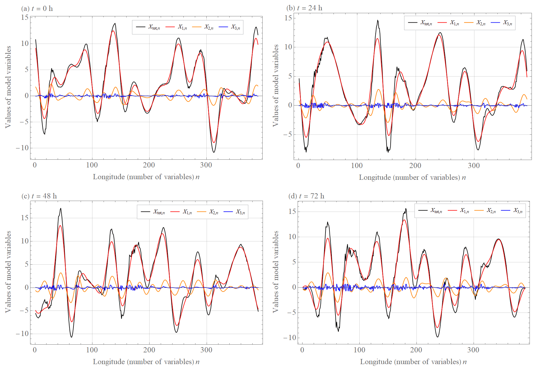
Figure 1(a) Initial conditions (after discarding a transient of 10 years) and values of variables () at days (b) one, (c) two, and (d) three of the L05-3 system (Eqs. 13–15) with the parameters N = 390, L = 13, J = 6, F = 15, b1 = 1, b2 = 10, c1 = 1, c2 = 1, I1 = 20, I2 = 10 calculated by a fourth-order Runge–Kutta method with a time step Δt = or 0.5 h.
For the L05-3 system (Eqs. 12–15), it is necessary to specify eight parameters. We tested that the values of coupling coefficients c1 and c2 do not affect the L05-3 system compared to the values of other parameters, and therefore for simplification c1 = 1 and c2 = 1. The parameter F=15 is set the same as for other L05 systems. For the medium-scale amplitude to be approximately 10 times smaller than the large-scale amplitude and the small-scale amplitude to be approximately 10 times smaller than the medium-scale amplitude and for the scales to have different oscillation rates (Fig. 1), the spatiotemporal scale factors are chosen as b1 = 1 and b2 = 10 and interval lengths I1 = 20 and I2 = 10. N = 390 turned out to be most suitable for the chaotic behavior of all three levels. In the following, we will present numerical results of the L05-3 system (Eqs. 12–15) with the parameters N = 390, L = 13, J = 6, F = 15, b1 = 1, b2 = 10, c1 = 1, c2 = 1, I1 = 20, and I2 = 10, calculated by a fourth-order Runge–Kutta method with a time step Δt = or 0.5 h. Initial conditions (, , , ), which should be free of transient effect, are chosen as final values of arbitrary values integrated for 175 200 steps or 10 years. Initial conditions and values of variables at days one, two, and three can be seen in Fig. 1.
3.1 Concepts to characterize scale-dependent error growth
In the pioneering papers of Aurell et al. (1996, 1997), a mathematical concept and a numerical scheme for the calculation of scale-dependent error growth was introduced, called the “finite size Lyapunov exponent”. Actually, Aruell et al. (1996) have already referred to the atmospheric predictability problem and named this as one motivation for their work. These papers triggered a set of follow-up publications where it was studied how scale-dependent error growth manifests itself in different models with intrinsic hierarchies such as models for fully developed turbulence like the shell model (Aurell et al., 1996) or how they can be used to study the issue of predictability (Boffetta et al., 1998; for a review see Cencili and Vulpiani, 2013). In brief, a finite size Lyapunov exponent can be defined as the ergodic average over phase space of the growth rate of perturbations of a given magnitude, where the growth rate is defined as the inverse of the time needed for the error magnitude to increase by a pre-defined factor.
In order to be able to investigate the data from the ECMWF forecasts as well, we use here a less rigorous approach: we measure the error amplitude after fixed time intervals. We then calculate the mean error amplitudes after fixed times, calculate the average growth rates during the last time interval, and can report the mean growth rates versus mean error magnitudes. Due to the fact that the conditioning is different, this is not the same as the calculation of the finite size Lyapunov exponent, but it reports similar properties of the system. However, our quantity is more appropriate for the forecast problem: the initial condition of a forecast has some small error compared to the unknown truth, and assuming a perfect model, we therefore calculate the average forecast error after a finite time.
3.2 Numerical scheme for scale-dependent error growth rates
In the following, we describe in more detail our numerical approach. By “error growth”, we denote the growth of errors in the initial conditions, which limit predictability if a system is chaotic. A numerical error growth experiment in a model system, therefore, consists of repeatedly generating a reference trajectory, which is considered to be the “truth” or verification, and a perturbed trajectory which is the numerical solution of the system for a perturbed initial condition (perfect model assumption). The time evolution of the difference vector between these two trajectories averaged over many repetitions then gives insight into the growth of prediction errors. In order for this scheme to be meaningful, we have to ensure that the reference trajectory is on the attractor of the system, that the repetition of this scheme samples the whole attractor with correct weights (the invariant measure), and that initial perturbations point already into the locally most unstable direction, since otherwise errors might even shrink on short timescales (this is also a relevant issue in ensemble forecasts and there its solutions are found in using bred vectors; Toth and Kalnay, 1997). We solve these issues in the following way: we first integrate the system over 10 years, starting from arbitrary initial conditions, and assume that after discarding this transient, the trajectory is on the attractor. We continue to integrate this single trajectory and consider segments of it as reference trajectories for error growth, i.e., the many reference trajectories are simply segments of one very long trajectory, which ensures not only that all these segments are located on the attractor, but that in addition, they sample the attractor according to the invariant measure. For the perturbed trajectories, we start with a random perturbation of the reference trajectory of very small amplitude and let this trajectory evolve over time before we start to determine its distance towards the reference trajectory. In other words, we discard some initial time interval of error growth from our study since this is affected by some complicated transient behavior before it starts to grow with the maximum Lyapunov exponent. However, due to the hierarchical nature of our model, the error growth with the maximal Lyapunov exponent will saturate already for rather small error amplitudes and will be replaced by slower error growth on larger scales, an effect which we will study in detail. The above-described scheme was originally introduced by Lorenz (1996).
In our system, the three spatial scales X1, X2, and X3 cannot be separated in terms of a coordinate transform but are intrinsically coupled and superimposed in the variables Xtot of the system. The initial conditions of the “reality” are called , from which one finds , , and through Eqs. (13)–(15). The initial values of the “prediction” are then , where e3,n(0) denotes the initial errors randomly selected from the normal distribution . Hence, these initial conditions differ only by the small perturbation e3,n(0). Since the state of the model Xtot is the sum over the three components, any arbitrary but small error with spatially uncorrelated components affects only . Only a spatially correlated initial error would appear in another component, but since this error would immediately propagate into the small-scale variables and then grow fastest in these, a perturbation with initial errors in is the only practical choice. From and Eq. (12) is integrated forward for 41.7 d (K = 2000 steps). In each time step k of the numerical integration, , and is obtained. The size of the error at a given time kΔt is , where , and . We perform M = 400 runs in order to calculate the average error growth. In each new run, the initial values are the last values of the previous run. The average initial error growth E(t) is defined as the geometric mean of the runs of the Euclidean distances between “reality” and “prediction”:
where . The initial transient behavior (0.7 d) of the average error growth E(t) is discarded. We do this since the random initial errors perturb the initial state off the attractor. On very short timescales, the perturbed trajectory relaxes back to the attractor (Brisch and Kantz, 2019; Bednář et al., 2014) so that the error does not grow. Only after this transient does one observe the characteristic error growth of the system. In real weather forecasts, the data assimilation scheme 4D-Var usually ensures that the (error-prone) analysis which is used as the initial condition of the forecast is on the attractor, and also in ensemble forecasts, the perturbations to the analysis are, for example, by the usage of bred vectors, done in a way that all ensemble members start on (or at least very close to) the attractor. As a result, we have numerical averages for the error growth as a function of time steps after perturbing the reference trajectories in the full phase space and for . We can convert these results into the error growth rate as a function of time, and into the error growth rate as a function of the error magnitude. Inspired by Anonymous Referee #1 (2021), we also performed for our model system an analysis in terms of the finite size Lyapunov exponent (Aurell et al. 1996). The results are qualitatively the same as found by our analysis, with small quantitative differences in the magnitude of the error growth rates (not shown here). As we discussed before, the ECMWF data can be only analyzed using our approach, and our approach is also more consistent with the performance of forecasts.
3.3 Functional forms for error growth rates
Let us first consider a classical low-dimensional chaotic system. If the initial errors were infinitesimal, one could follow their growth for infinite times and define the maximal Lyapunov exponent of the system as , with a time- and error-independent growth rate Λ. This exponential growth is associated with single scale systems, infinitesimal initial error, and the early part of the error growth (Bednář et al., 2014). In reality, since the initial perturbation is non-infinitesimal, the exponential error growth will cross over to a constant: the distance between the “true” and the perturbed trajectories cannot become larger than the largest distance on the attractor. Hence, for large times. the average “error” is then the average distance of two arbitrary points on the attractor, averaged over the invariant measure. In order to take this saturation effect into account, we use the extended exponential law for the error growth rate: , where E∞ is the saturation value of the respective error. Notice that this extension does not involve any free parameter other than the measurable saturation value E∞.
We calculate the error growth rate in our L05-3 system using the method of Sprott (2006) (, k=10 and k=100, M=105). In the following, Eτ(t) denotes mean over many initial conditions of the Euclidian distances between the “true” and the perturbed trajectories at a time t after initializing the perturbation, measured in the subspace of the coordinates τ, where . Numerically, we find , , , and (units). We determine the maximal Lyapunov exponents in all four cases and find the values ≈ 2.5 (d)−1 and ≈ 2 (d)−1. The similarity of the values Λtau,theor for all levels indicates that they are coupled, so that the maximal Lyapunov exponent when calculated in the double limit E0→0 and t→∞ shows up in arbitrary subsystems. These values must not be confused with the Lyapunov exponents characterizing the different levels which we will calculate later: the evolution of the errors Eτ can always be studied in a way to see the largest exponent of the system (done here), but also in a way to see a value which would be the exponent of the corresponding sub-system if one were able to isolate this. In the context of the coupled system, these sub-system exponents are just some other positive exponents of the full system, since Eq. (12) in total has, as every dynamical system, as many Lyapunov exponents as it has degrees of freedom (here N = 390), where several of these can be positive.
The L05-3 system is designed with three spatial and temporal scales, so the error growth rate is expected to be a function of the error magnitude E: after the small-scale errors are no longer growing, the large-scale errors continue to grow at a lower rate. Brisch and Kantz (2019) described this dependence by a power law:
with an exponent σ and a coefficient a>0. By integrating Eq. (17) over time, the power law dependence of the error growth rate on the error magnitude translates into a power law growth of errors over time:
Similar to the exponential law, this power law does not take the saturation of errors at their largest scale into account. We, therefore, multiply the right hand side by and arrive at the extended power law:
Unfortunately, the time integration in order to arrive at an expression of Ew(t) cannot be done analytically but numerically once the parameters are fixed.
A different description of scale-dependent error growth rate was proposed by Zhang et al. (2019), namely a quadratic model which we write down directly in its extended form containing the saturation effect:
where α is a synoptic-scale error growth rate and β is an upscale error growth rate from small-scale processes, which was originally designed to describe model error (Savijarvi, 1995; Dalcher and Kalnay, 1987). By integrating Eq. (20) over time, we find
When removing the saturation factor in Eq. (21), then it is what was called the quadratic model,
with the time evolution of the error
which is suitable for the first few days of the error growth.
To summarize, we can test the validity of the following laws for scale-dependent error growth rates and for the error growth over time: a constant Lyapunov exponent and hence an exponential error growth, as is expected for the initial time of very small initial errors in a low-dimensional chaotic system; the extension of this behavior with a saturation factor expected to be valid for all times in a low-dimensional chaotic system; the (extended) quadratic law proposed in Zhang et al. (2019); and the (extended) power law growth proposed in Brisch and Kantz (2019).
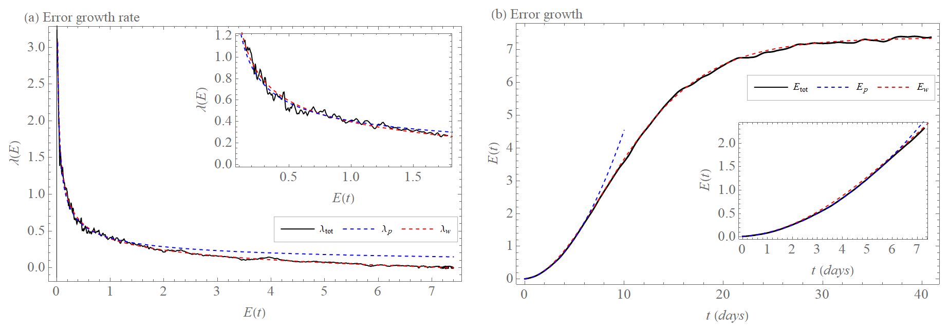
Figure 2(a) Error growth rate λtot(E)of the L05-3 system (black). Power law λp(E) (Eq. 19) with the exponent σ=0.5 and the coefficient a=0.41 (units0.5 d−1) (λtot,p(E), blue, dashed) and extended power law λw(E) (Eq. 26) with the exponent σ=0.47, the coefficient a=0.46 (units0.47 d−1), and E∞=7.36 (units) (λtot,w(E), red, dashed) that approximate λtot(E). (b) Error growth Etot(t) (Eq. 17) (black), solution Etot,p(t) (blue, dashed) of λtot,p(E) (Eq. 19), and numerical solution of λtot,w(E) (red, dashed).

Figure 3(a) Error growth rate λtot(E) of the L05-3 system (black). Quadratic model λr(E) (Eq. 22) with α=0.25 (d−1) and β=0.13 (units per day) (λtot,p(E), blue, dashed) and extended quadratic model λq(E) (Eq. 20) with α=0.2 (d−1), the coefficient β=0.19 (units per day), and E∞=7.3 (units) (λq,w(E), red, dashed) that approximate λtot(E). (b) Error growth Etot(t) (Eq. 17) (black), solution Etot,r(t) (blue, dashed) of λtot,r(E) (Eq. 22), and solution Etot,q(t) (blue, dashed) of λtot,q(E) (Eq. 21) (red, dashed).

Figure 4(a) Error growth rate λ3(E)of the L05-3 system's X3 scale (black). Extended exponential growth λe(E) (Eq. 24) with Λ3 = 3.6 (d−1) and = 0.06 (units) (λ3,e(E), red, dashed) and extended power law λw(E) (Eq. 26) with the exponent σ=0.75, the coefficient a=0.13 (units0.75 d−1), and = 0.3 (units) (λ3,w(E), blue, dashed) and ≈ 2.5 (d−1) (Sprott's, 2006, method, orange, dotted). (b) Error growth rate λ2(E) of the L05-3 system's X2 scale (black). Extended exponential growth λe(E) (Eq. 24) with Λ2 = 0.8 (d−1) and = 0.55 (units) (λ2,e(E), red, dashed) and extended power law λw(E) (Eq. 26) with the exponent σ=0.44, the coefficient a = 0.25 (units0.44 d−1), and = 1.4 (units) (λ2,w(E), blue, dashed) and error growth rate λ3(E) of the L05-3 system's X3 scale (orange). (c) Error growth rate λ1(E)of the L05-3 system's X1 scale (black). Extended exponential growth λe(E) (Eq. 24) with Λ1 = 0.28 (d−1) and = 6.1 (units) (λ1,e(E), red, dashed) and extended power law λw(E) (Eq. 26) with the exponent σ = 0.5, the coefficient a = 0.43 (units0.5 d−1), and = 6.6 (units) (λ1,w(E), blue, dashed). (d) Error growth rate λτ(E) where τ = tot (black, thin), τ = 1 (red, thin), τ = 2 (orange, thin), τ = 3 (blue, thin). Extended power law λτ,w(E) where τ = tot (black), τ = 1 (red), τ = 2 (orange) with (orange, dashed–dotted), τ = 3 (blue) with (blue, dashed–dotted). Power law λtot,p(E) (black, dashed). Extended exponential growth λτ,e(E) where τ = 1 (red, dashed) with Λ1 (red, dotted), τ = 2 (orange, dashed) with Λ2 (orange, dotted), τ = 3 (blue, dashed) and Λteor (black, dotted).
In Figs. 2–4, we present the numerical results of the error growth over time of the errors Eτ(t) for , and the corresponding error growth rates as a function of the error magnitude.
The power law λp(E) (Eq. 17) approximates the L05-3 system error growth rate λtot(E) in the interval (Fig. 2a). For larger errors, there is no “next level” of the hierarchy any more, so that the power law evidently cannot be valid. For , the empirical error growth rate λtot(E) (Fig. 2a) decreases much faster than the power λp(E), due to saturation of the errors at E∞. Hence, the power law Ep(t) (Eq. 18) yields a good approximation of L05-3 system error growth Etot(t) only in the early part of the growth within 6 d (Fig. 2b), where we find the numerical values σ=0.5 and a=0.41 (units0.5 d−1). This power law needs to be corrected on times beyond 6 d in order to be able to model the saturation of errors, called the extended power law above. Inserting the numerically observed saturation value E∞=7.4, a fit of λw(E) Eq. (19) yields σ=0.47, a=0.46 (units0.47 d−1). With this extension, we are able to suitably approximate the L05-3 system error growth (Fig. 2a) on the entire range of errors. The numerical time integration of Eq. (19) approximates correspondingly well the L05-3 system error growth Etot(t) from the initial conditions E0 to the limit (saturated) value Etot,∞ (Fig. 2b).
We also fit the quadratic model λr(E), Eq. (22), to the numerically obtained L05-3 system error growth rate λtot(E). It can reproduce the error growth rate in the interval as well, but not as accurately as the power law (Fig. 3a). For larger errors in the interval , the quadratic model λr(E) decreases more slowly than the L05-3 system error growth rate λtot(E) and the power law λp(E) (Figs. 3a and 2a). The solution of the quadratic model for the time evolution of the error, Er(t) (Eq. 23), with α=0.25 (d−1) and β=0.13 (units per day) determined from the approximation is similar to Ep(t) with a given coefficient and exponent, but it does not approximate the data as accurately (Fig. 3b). The factor (1−E∞) with E∞=7.3 in the extended quadratic model, Eq. (20), yields a much better approximation along the entire time interval, (Fig. 3a), but it is slightly less accurate than the extended power law in the interval . This inaccuracy is significant for the solution of the extended quadratic model Eq(t) (Eq. 21) with α=0.2 (d−1) and β=0.19 (units per day) determined from the approximation, where the early part of growth is the least similar to error growth Etot(t) (Fig. 3b).
3.3.1 Self-consistent explanation of the observed approximate power law
Brisch and Kantz (2019) derived the value of the exponent σ of the power law Eq. (17) from other system properties. They argue that the power law is a result of the superposition of the error growth on different spatial scales with different growth rates. Translated into our L05-3 system it should work as follows: the small-scale error growth E3(t) should follow the (extended) exponential growth (solution of , with Λ3 and a saturation scale E3,∞. After its saturation, the medium-scale error continues to grow, but with a lower rate Λ2, and will saturate at a larger scale E2,∞. Beyond that, the total error growth can only be driven by the growth of the large-scale errors with an even slower growth rate Λ1 and saturation scale E1,∞. If the model is designed such that Λ2=cΛ1 and Λ3=c2Λ1, while and , then it was argued that the exponent of the power law should be .
The model of Brisch and Kantz (2019) was constructed of weakly coupled identical sub-systems, with additional scaling parameters for the amplitude and time of the different subsystems. Therefore, there were rather well defined error growth rates Λτ, , and it was easily possible to tune these so that and . In our L05-3 model, all this is not the case. The advantage of our model, however, is that it is much closer to the phenomenology of an atmospheric model: in a single field Xtot, we observe both large-scale and small-scale structures, and we observe both fast and slow motion.
In the L05-3 model, we have determined the error growth of a given level by the study of the distance between reference trajectories and perturbed trajectories in the corresponding coordinates Xτ, ; see Fig. 4. It is straightforward to identify the saturation values Eτ,∞. We describe here how we find approximate values for the growth rates Λτ in the extended exponential law ( from our numerics. We can then determine c and b and hence a theoretical value for σ, which we will compare to the numerical fit.
By Sprott's method (Sprott, 2006) we calculate the error growth rates of the three levels separately and the total error growth rate. As one can see in Fig. 4, λτ(E) can be well described by the extended power law λw(E) on the whole range of E for all τ. The individual contributions of the levels (scales) Xτ, to the error growth rates λτ(E) are then identified as parts that fulfill the extended exponential growth λe(E). Numerically, we identify the following values: the extended growth rates are Λ3=3.6 (d−1), Λ2=0.8 (d−1), and Λ1=0.28 (d−1). The corresponding saturation scales are determined as (units), (units), and (units). The values for levels τ=2 are extracted from the range where the effect of λ3(E) is no longer present (Fig. 4b), while for τ=1 we consider the late stage of the error growth rate λ1(E) (Fig. 4c). Following the arguments from above, we derive σ as where and . We get the same value of where , and , even though b1≠b2 and c1≠c2. Note that c2 uses Λ3,teor instead of Λ3. This is because Λ3 should be computed from the ranges where E and t are small/short but which include some transient behavior (Fig. 4a), and therefore Λ3,teor is a more appropriate value.
These derived values for σ are in perfect agreement with the empirical fit of the extended power law λw(E), which yields σ=0.47, and it is close to the value σ=0.50 of the power law λp(E) without the saturation effect.
The coupling of the levels has the consequence that one cannot define the Lyapunov exponents for the individual levels in a mathematically rigorous way. We calculated them as (d−1) at and (d−1) at using the extended exponential law. It is well justified to use these to determine the exponent σ. However, they do not fit the error growth rate , , Fig. 4d). Instead, a fit to λtot(E) yields (d−1) in the limit value of medium-scale error growth and (d−1) in the limit value of small-scale error growth (Fig. 4d). If we approximate the values and by the power law λp(E) with the exponent σ=0.5, we get the coefficient a=0.2 (units0.5 d−1), and by the power law λp(E) with the exponent σ=0.47, we get a=0.21 (units0.47 d−1). These power laws should describe the error growth of the system without coupling (the extended power law was not used because is negligible in this area), and if we compare these values with the values of the power laws (λtot,p(E): σ=0.5, a=0.41 (units0.5 d−1), λtot,w(E): σ=0.47, a=0.46 (units0.46 d−1)) that approximate the error growth rate of the L05-3 system λtot(E) (the system with coupling), we find that the value of the coefficient a changed. We, therefore, conclude that the coefficient a is subject to the degree of coupling of the system.
Values α=0.25 (d−1) for the quadratic model λr(E) (Eq. 22) and α=0.2 (d−1) for the extended quadratic model λq(E) (Eq. 20) should describe the synoptic-scale error growth rate (Zhang et al., 2019; Zhang and Sun, 2020). For the L05-3 system, it is Λ1=0.28(d−1) obtained from the approximation by the extended exponential growth () for X1. We can see that Λ1 is closer to α from the quadratic model λr(E), but none of α describes Λ1 exactly. Values β=0.13 (units per day) and β=0.19 (units per day) that according to Zhang et al. (2019) and Zhang and Sun (2020) should describe upscale error growth rate from small-scale processes could not be identified or described in the L05-3 system.

Figure 5The error growth rate λEFS(E) and error growth EEFS(t) of the ECMWF forecasting system's 500 hPa geopotential height values (Northern Hemisphere, 20–90∘) calculated as differences between two operational forecasts issued with 1 d lag but valid on the same day (black), approximation by the extended power law λw(E) (Eq. 26) and Ew(t) (Eq. 27) (red, dashed), and approximation by the extended quadratic model λq(E) (Eq. 20) and Eq(t) (Eq. 21) (blue, dashed). (a, b) Annual average of 2000, λEFS,w(E) and EEFS,w(t) with σ = 0.28, a = 1.1 (m0.28 d−1), and E∞ = 115 (m), λEFS,p(E) and EEFS,p(t) with α = 0.32 (d−1) and β = 3.2 (m d−1) and E∞ = 110 (m). (c, d) Annual average of 2010, λEFS,w(E) and EEFS,w(t) with σ = 0.17, a = 0.8 (m0.17 d−1), and E∞ = 114 (m), λEFS,p(E) and EEFS,p(t) with α = 0.4 (d−1) and β = 2 (m d−1) and E∞ = 111 (m).
The error growth EEFS(t) of the ECMWF forecasting system's 500 hPa geopotential height values (Magnusson, 2013) is calculated (Magnusson and Kallen, 2013) as annual averages over the Northern Hemisphere (20–90∘) obtained daily from 1 January 1986 to 31 December 2011. As “errors” one uses the differences between two operational forecasts issued with 1 d lag for the same day, in order to eliminate the effects of model errors. Specifically, we evaluate these for 27 different lead times and used the following time intervals in hours: 0–24, 6–30, 12–36, 18–42, 24–48, 30–54, 36–60, 42–66, 48–72, 54–78, 60–84, 66–90, 72–96, 78–102, 84–108, 90–114, 96–120, 108–132, 120–144, 132–156, 144–168, 156–180, 168–192, 180–204, 192–216, 204–228, 216–240. Detailed information about calculating the error growth of the ECMWF forecasting system can be found in Lorenz (1982). The error growth rate with Δt=6 h for the first 17 time steps and Δt = 12 h for the remaining 10 time steps and the error growth EEFS(t) are calculated between the first and tenth day. The differences 0–24, 6–30, 12–36 are discarded because λEFS(E) for these differences is either increasing or constant due to transient behavior; see Fig. 5.
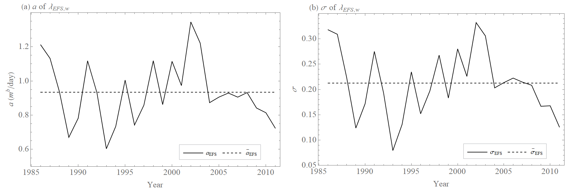
Figure 6Values of coefficients a (a) and exponents σ (b) of the extended power law λw(E) (Eq. 26) approximated from annual averages of the error growth rate λEFS(E) of the ECMWF forecasting system's 500 hPa geopotential height values (Northern Hemisphere, 20–90∘) calculated as differences between two operational forecasts issued with 1 d lag but valid on the same day (black) and the average value of coefficients = 0.93 ± 0.18 mσ d−1 and exponents = 0.21 ± 0.07 over all years (black, dashed).
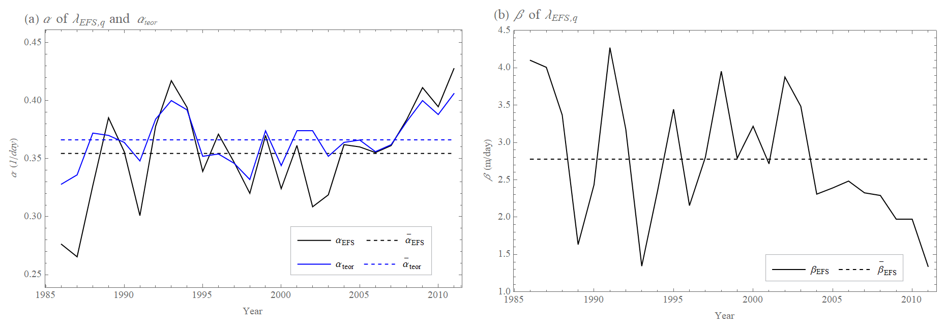
Figure 7Values of parameters α (a) and β (b) of the extended quadratic model λq(E) approximated from annual averages of the error growth rate λEFS(E) of the ECMWF forecasting system's 500 hPa geopotential height values (Northern Hemisphere, 20–90∘) calculated as differences between two operational forecasts issued with 1 d lag but valid on the same day (black), the average value of parameters = 0.35 ± 0.04 d−1 and = 2.8 ± 0.9 m d−1 over all years (black, dashed) and theoretical value of αteor (blue) and its average value = 0.37 ± 0.02 d−1 (blue, dashed) over all years determined by Bednář et al. (2021).
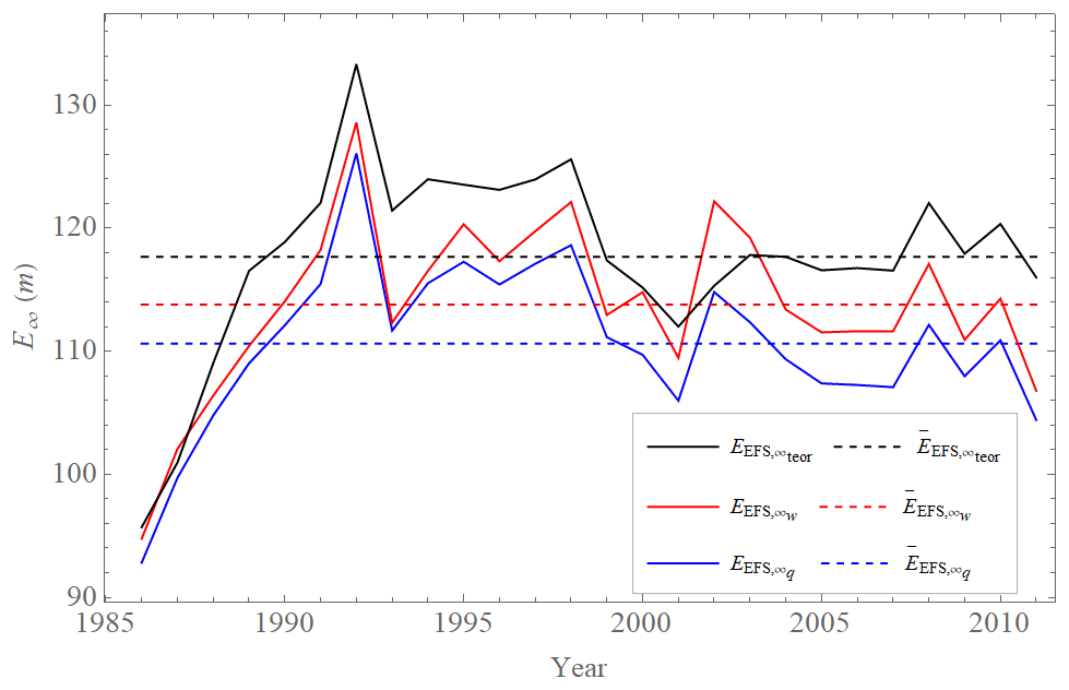
Figure 8Values of limit (saturated) values of the extended power law λw(E) (red), of the extended quadratic model λq(E) (blue), and theoretical value determined by Bednář et al. (2021) (black) approximated from annual averages of the error growth rate λEFS(E) of the ECMWF forecasting system's 500 hPa geopotential height values (Northern Hemisphere, 20–90∘) calculated as differences between two operational forecasts issued with 1 d lag but valid on the same day. The average value of = 114 ± 7 m (red, dashed), = 111 ± 7 m (blue, dashed), and = 118 ± 7 m (black, dashed).
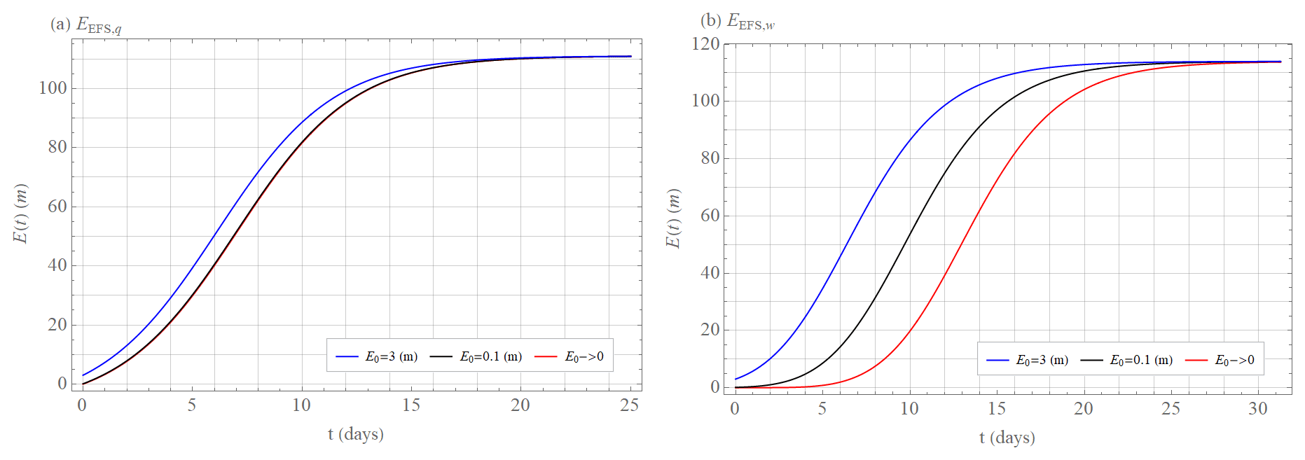
Figure 9(a) The solution of the extended quadratic model Eq(t) with parameters = 0.35 d−1 and = 2.8 m d−1, limit (saturated) value = 111 m and with initial errors E0 = 3 m (blue), E0 = 0.1 m (black), and E0→0 (red). (b) The solution of the extended power law Ew(t) with the coefficient = 0.93 mσ d−1, exponent = 0.21, limit (saturated) value = 114 m and with initial errors E0 = 3 m (blue), E0 = 0.1 m (black), and E0→0 (red). Bar above parameters and limit value means averages over approximations of λq(E) and λw(E) from annual averages of the error growth rate λEFS(E) of the ECMWF forecasting system's 500 hPa geopotential height values (Northern Hemisphere, 20–90∘) calculated as differences between two operational forecasts issued with 1 d lag but valid on the same day.
Despite these missing parts of the error growth EEFS(t), Bednář et al. (2021) showed that the extended quadratic model Eq(t) Eq. (21) is more accurate than the extended exponential growth (solution of ). Because EEFS(t) calculated in the abovementioned way should be insensitive to any model error which therefore can not affect the error growth, the extended quadratic model parameter β describes the effect of small-scale processes, which justifies considering the error growth rate λEFS(E) for all annual averages as scale-dependent and also approximating it by the extended power law λw(E) Eq. (19). The quadratic model λr(E) (Eq. 22) and the power law λp(E) (Eq. 17) cannot be used due to the lack of an early part of the error growth EEFS(t). The extended power law λw(E) (Eq. 19) matches well with the annual averages of the error growth rate λEFS(E) of the ECMWF forecasting system (Fig. 5) with the values of the exponent σEFS displayed in Fig. 6b ( = 0.21 ± 0.07), the value of the coefficient aEFS shown in Fig. 6a ( = 0.93 ± 0.18 m0.21 d−1), and with the limit (saturated) values displayed in Fig. 8 ( = 114 ± 7 m). Exponents σEFS, coefficients aEFS, and limit values do not have significant trends over the years (Figs. 6 and 8). The extended quadratic model λq(E) Eq. (20) approximates annual averages of the error growth rate λEFS(E) of the ECMWF forecasting system (Fig. 5) with the values of the parameter αEFS shown in Fig. 7a ( = 0.35 ± 0.04 d−1), the value of the parameter βEFS displayed in Fig. 7b ( = 2.8 ± 0.9 m d−1), and with the limit (saturated) values displayed in Fig. 8 ( = 111 ± 7 m). Again, parameters αEFS and βEFS and limit values do not have significant trends over the years (Figs. 7 and 8). The approximations by the extended quadratic model λq(E) and the extended power law λw(E) differ in parts where data are not available (Fig. 5). The limit values and initial errors of the extended power law are greater than the limit values and initial errors of the extended quadratic model (Figs. 5 and 8). If we set the initial errors of both approximations to the same value, the error growth of the extended quadratic model EEFS,q(t) approximation would grow faster and would reach the limit value EEFS,∞ earlier than the error growth of the power law EEFS,w(t). This difference is more significant when E0→0. Of particular interest is the limit of predictability. We, therefore, study the time when the error E(t) reaches 95 % of the limit error E∞ for the size of the initial error E0 ≈ 3 m, which is an accepted value for current global operational numerical weather prediction (NWP) models (Zhang et al., 2019). The limit time is 14 d for the extended quadratic model when using the abovementioned parameter values for , , and (Fig. 9a). For the extended power law , using the above listed values for the exponent , coefficient , and limit values , it is 15 d (Fig. 9b). When the size of the initial error E0 is reduced to E0 ≈ 0.1 m, which is realistic for the current global experimental NWP models (Zhang et al., 2019), this limit time is 15 d for the extended quadratic model (Fig. 9a), and 18 d for the extended power law (Fig. 9b). Both models have an intrinsic predictability limit even if the size of the initial error E0→0, which is 15 d for the extended quadratic model (Fig. 9a) and 22 d for the extended power law (Fig. 9b).
We designed a three-level (three-scale) system (L05-3; Eqs. 12–15) with the parameters N=390, L=13, J=6, F=15, b1=1, b2=10, c1=1, c2=1, I1=20, I2=10. These parameters were chosen in such a way that all levels behave chaotically, i.e., the largest Lyapunov exponents of each level is positive, and that all levels have a significant difference in amplitudes and fluctuation rates (Fig. 1). In this system, the error growth rates λτ(E) and the error growths as a function of time Eτ(t) were calculated for the system as a whole (τ=tot) and for the different levels (. We fitted the numerically obtained results by the power law λp(E) (Eq. 17), the extended power law λw(E) (Eq. 19), the quadratic hypothesis λr(E) (Eq. 22), the extended quadratic hypothesis λq(E) (Eq. 20), and their corresponding time integrations E(t). Without the saturation terms both the power law and the quadratic hypothesis fail to provide good fits for larger errors or longer times (Figs. 2 and 3) but are reasonable for the early parts of error growth when the initial error is small. Indeed, with our type of numerical analysis, we are unable to reach the very small scales where the error growth rate saturates at the proper Lyapunov exponent of the system which we estimate to be about 2.5 d−1 but instead are faced by an overshooting of the initial error growth.
The quadratic hypothesis does not provide an as good a fit as the extended power law does. Its parameter β that according to Zhang et al. (2019) and Zhang and Sun (2020) should describe the upscale error growth rate from small-scale processes could not be identified or described in the L05-3 system. In contrast, the extended power law λw(E) and Ew(t) with the exponent σ=0.47, the coefficient a=0.46 (units0.47 d−1), and E∞=7.36 best describes the error growth rate λtot(E) and the error growth Etot(t) of the L05-3 system on the whole range of times and error magnitudes. The Brisch and Kantz (2019) definition of the exponent σ was confirmed and extended to cases when c1≠c2 (c is the ratio of the rapidness of a smaller scale compared to the rapidness of a larger scale) and b1≠b2 (b is the ratio of a smaller-scale amplitude compared to a larger-scale amplitude) for . It was shown that the coefficient a determines the degree of the system's coupling because the same value of the exponent σ is valid for the same system with and without coupling.
We also checked the appropriateness of the extended quadratic hypothesis and the extended power law to describe the error growth rate λEFS(E) and the error growth over time EEFS(t) of the ECMWF forecasting system's 500 hPa geopotential height values over the 1986 to 2011 period. Their behaviors differ in parts where data are not available (Fig. 5), while they agree quite well and both describe the numerical observations on the main part of the data. Therefore, it is not possible to assess which approximation is the more appropriate one for the description of the entire length of λEFS(E) and EEFS(t) from the initial to the limit (saturated) error. One might argue, however, that because we can observe the similarities of the differences between the data and the approximations in both systems ( (Fig. 8) and ; (Fig. 7) and ), the extended power law λw(E) is also a valid description of the ECMWF forecasting system. From the average of the fit parameters over many years we calculate that the intrinsic limit to predictability is 22 d in the idealized case of perfect initial conditions, which is in nice agreement with Krishnamurthy (2019).
The ECMWF forecasting system dataset was obtained from the personal repository of Linus Magnusson (Magnusson, 2013). The L05-3 system dataset, products from the ECMWF forecasting system dataset, codes, and figures were conducted in Wolfram Mathematica, and they are permanently stored at https://doi.org/10.17605/OSF.IO/2GC9J (Bednář, 2021).
HB proposed the idea, carried out the experiments, and wrote the paper. HK supervised the study and co-authored the paper.
The contact author has declared that neither they nor their co-author has any competing interests.
Publisher's note: Copernicus Publications remains neutral with regard to jurisdictional claims in published maps and institutional affiliations.
The authors are grateful to Linus Magnusson for offering a dataset (ECMWF forecasting system) from his personal repository.
This research has been supported by the Czech Science Foundation (grant no. 19-16066S).
The article processing charges for this open-access publication were covered by the Max Planck Society.
This paper was edited by Ignacio Pisso and reviewed by two anonymous referees.
Anonymous Referee #1: Comment on gmd-2021-256, https://doi.org/10.5194/gmd-2021-256-RC1, 2021.
Aurell, E., Boffetta, G., Crisanti, A., Paladin, G., and Vulpiani, A.: Growth of noninfinitesimal perturbations in turbulence, Phys. Rev. Lett., 77, 1262, https://doi.org/10.1103/PhysRevLett.77.1262 1996.
Aurell, E., Boffetta, G., Crisanti, A., Paladin, G., and Vulpiani, A.: Predictability in the large: an extension of the concept of Lyapunov exponent, J. Phys. A-Math. Gen., 30, 1–26, https://doi.org/10.1088/0305-4470/30/1/003, 1997.
Bednář, H.: Prediction error growth in a more realistic atmospheric toy model with three spatiotemporal scales, OSF [code and data set] https://doi.org/10.17605/OSF.IO/2GC9J, 2021.
Bednář, H., Raidl, A., and Mikšovský, J.: Initial Error Growth and Predictability of Chaotic Low-dimensional Atmospheric Model, IJAC, 11, 256–264, https://doi.org/10.1007/s11633-014-0788-3 2014.
Bednář, H., Raidl, A., and Mikšovský, J.: Recalculation of error growth models' parameters for the ECMWF forecast system, Geosci. Model Dev., 14, 7377–7389, https://doi.org/10.5194/gmd-14-7377-2021, 2021.
Boffetta, G., Giuliani, P., Paladin, G., and Vulpiani, A.: An Extension of the Lyapunov Analysis for the Predictability Problem, J. Atmos. Sci., 23, 3409–3416, https://doi.org/10.1175/1520-0469(1998)055<3409:AEOTLA>2.0.CO;2 1998.
Brisch, J. and Kantz, H.: Power law error growth in multi-hierarchical chaotic system-a dynamical mechanism for finite prediction horizon, New J. Phys., 21, 1–7, https://doi.org/10.1088/1367-2630/ab3b4c 2019.
Cencini, M. and Vulpiani, A: Finite Size Lyapunov Exponent: Review on Applications, J. Phys. A, 46, 254019, https://doi.org/10.1088/1751-8113/46/25/254019 2013.
Dalcher, A. and Kalnay, E.: Error growth and predictability in operational ECMWF analyses, Tellus A, 39, 474–491, https://doi.org/10.1111/j.1600-0870.1987.tb00322.x 1987.
Harlim, J., Oczkowski, M., Yorke, J. A., Kalnay, E., and Hunt, B. R.: Convex error growth patterns in a global weather model, Phys. Rev. Lett., 94, 228501, https://doi.org/10.1103/PhysRevLett.94.228501, 2005.
Krishnamurthy, V.: Predictability of Weather and Climate, Earth Space Sci., 6, 1005–1318, https://doi.org/10.1029/2019EA000586 2019.
Lorenz, E. N.: Deterministic nonperiodic flow, J. Atmos. Sci., 20, 130–141, https://doi.org/10.1175/1520-0469(1963)020<0130:DNF>2.0.CO;2 1963.
Lorenz, E. N.: The predictability of a flow which possesses many scales of motion, Tellus, 21, 289–307, https://doi.org/10.1111/j.2153-3490.1969.tb00444.x 1969.
Lorenz, E. N.: Atmospheric predictability experiments with a large numerical model, Tellus, 34, 505–513, https://doi.org/10.1111/j.2153-3490.1982.tb01839.x 1982.
Lorenz, E. N.: Predictability: a problem partly solved, in: Predictability of Weather and Climate, edited by: Palmer, T. and Hagedorn, R., Cambridge University Press, Cambridge, UK, 1–18, https://doi.org/10.1017/CBO9780511617652.004 1996.
Lorenz, E. N.: Designing chaotic models, J. Atmos. Sci., 62, 1574–1587, https://doi.org/10.1175/JAS3430.1 2005.
Magnusson, L.: Factors Influencing Skill Improvements in the ECMWF Forecasting System, available from personal repository: linus.magnusson@ecmwf.int [data set], 2013.
Magnusson, L. and Kallen, E.: Factors Influencing Skill Improvements in the ECMWF Forecasting System, Mon. Weather Rev., 141, 3142–3153, https://doi.org/10.1175/MWR-D-12-00318.1 2013.
Palmer, T. N., Döring, A., and Seregin, G.: The real butterfly effect, Nonlinearity, 27, 9, https://doi.org/10.1088/0951-7715/27/9/R123, 2014.
Savijarvi, H.: Error Growth in a Large Numerical Forecast System, Mon. Weather Rev., 123, 212–221, https://doi.org/10.1175/1520-0493(1995)123<0212:EGIALN>2.0.CO;2 1995.
Shukla, J.: Seamless prediction of weather and climate: A new paradigm for modeling and prediction research, US NOAA Climate Test Bed Joint Seminar Series, NCEP, https://www.nws.noaa.gov/ost/climate/STIP/FY09CTBSeminars/shukla_021009.pdf (last access: 20 June 2021), 2009.
Sprott, J. C.: Chaos and Time-series Analysis, Oxford University Press, New York, USA, 2006.
Toth, Z. and Kalnay, E.: Ensemble forecasting at NMC: The generation of perturbations, B. Am. Meteorol. Soc., 74, 2317–2330, https://doi.org/10.1175/1520-0477(1993)074<2317:EFANTG>2.0.CO;2 1993.
Toth, Z. and Kalnay, E.: Ensemble forecasting at NCEP and the breeding method, Mon. Weather Rev., 12, 3297–3319, https://doi.org/10.1175/1520-0493(1997)125<3297:EFANAT>2.0.CO;2 1997.
Zhang, F. and Sun, Q.: A New Theoretical Framework for Understanding Multiscale Atmospheric Predictability, J. Atmos. Sci., 77, 2297–2309, https://doi.org/10.1175/JAS-D-19-0271.1 2020.
Zhang, F., Sun, Q., Magnusson, L., Buizza, R., Lin, S. H., Chen J. H., and Emanuel K.: What is the Predictability Limit of Multilatitude Weather, J. Atmos. Sci., 76, 1077–1091, https://doi.org/10.1175/JAS-D-18-0269.1 2019.