Lossy checkpoint compression in full waveform inversion: a case study with ZFPv0.5.5 and the overthrust model

This paper proposes a new method that combines checkpointing methods with error-controlled lossy compression for large-scale high-performance full-waveform inversion (FWI), an inverse problem commonly used in geophysical exploration. This combination can significantly reduce data movement, allowing a reduction in run time as well as peak memory.

In the exascale computing era, frequent data transfer (e.g., memory bandwidth, PCIe bandwidth for GPUs, or network) is the performance bottleneck rather than the peak FLOPS of the processing unit.

Like many other adjoint-based optimization problems, FWI is costly in terms of the number of floating-point operations, large memory footprint during backpropagation, and data transfer overheads. Past work for adjoint methods has developed checkpointing methods that reduce the peak memory requirements during backpropagation at the cost of additional floating-point computations.

Combining this traditional checkpointing with error-controlled lossy compression, we explore the three-way tradeoff between memory, precision, and time to solution. We investigate how approximation errors introduced by lossy compression of the forward solution impact the objective function gradient and final inverted solution. Empirical results from these numerical experiments indicate that high lossy-compression rates (compression factors ranging up to 100) have a relatively minor impact on convergence rates and the quality of the final solution.

1 Introduction

Full-waveform inversion (FWI) is an adjoint-based optimization problem used in seismic imaging to infer the Earth's subsurface structure and physical parameters (Virieux and Operto, 2009). Here, a partial-differential equation (PDE) describing the propagation of a wave is solved repeatedly, while modifying the estimate of the physical properties of the system so that a simulated signal matches the signal recorded in a physical experiment. The compute and memory requirements for this and similar PDE-constrained optimization problems can readily push the world's top supercomputers to their limits. Table 1 estimates the computational requirements of an FWI problem on the Society of Exploration Geophysicists (SEG) Advanced Modelling Program (SEAM) model (Fehler and Keliher, 2011). Although the grid-spacing and time step interval depends on various problem-specific factors, we can do a back-of-the-envelope calculation to appreciate the scale of FWI. To estimate the number of operations per grid point, we use the acoustic anisotropic equation in a Tilted-Transverse Isotropic medium (Zhang et al., 2011), which is commonly used today in commercial FWI. Such a problem would require almost 90 d of continuous execution at 1 PFLOP s⁻¹. The memory requirements for this problem are also prohibitively high. As can be seen in Table 1, the gradient computation step is responsible for this problem's high memory requirement, and the focus of this paper is to reduce that requirement.

The FWI algorithm is explained in more detail in Sect. 2. It is important to note that despite the similar terminology, the checkpointing we refer to in this paper is not done for resilience or failure recovery. This is the checkpointing from automatic-differentiation theory, with the objective of reducing the memory footprint of a large computation by trading recomputation for storage. This checkpointing occurs completely in memory (i.e., RAM), and the discussion in this paper is orthogonal to any issues around disk input and output.

Table 1 Estimated computational requirements of a full waveform inversion problem based on the SEAM model (Fehler and Keliher, 2011), a large-scale industry standard geophysical model that is used to benchmark FWI. Note that real-world FWI problems are likely to be larger.

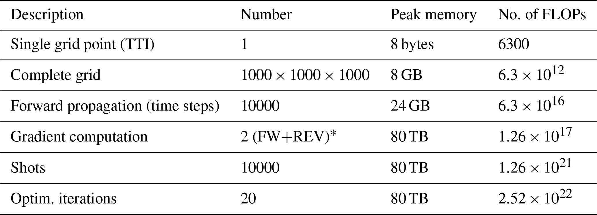
^* A gradient computation involves a forward simulation followed by a reverse/adjoint computation. For simplicity we assume the same size of computation during the forward/adjoint pass.

1.1 FWI and other similar problems

FWI is similar to other inverse problems like brain-imaging (Guasch et al., 2020), shape optimization (Jameson et al., 1998), and even training a neural network. When training a neural network, the activations calculated when propagating forward along the network need to be stored in memory and used later during backpropagation. The size of the corresponding computation in a neural network depends on the depth of the network and, more importantly, the input size. We assume the input is an image for the purpose of this exposition. For typical input image sizes of less than 500×500 px, the computation per data point is relatively small (compared to FWI), both in the number of operations and memory required. This is compensated by processing in mini-batches, where multiple data points are processed at the same time. This batch dimension's size is usually adjusted to fill up the target hardware to its capacity (and no more). This is the standard method of managing the memory requirements of a neural network training pipeline. However, for an input image that is large enough or a network that is deep enough, it is seen that the input image, network weights, and network activations together require more memory than available on a single node, even for a single input image (batch size =1). We previously addressed this issue in the context of neural networks (Kukreja et al., 2019b). In this paper we address the same issue for FWI.

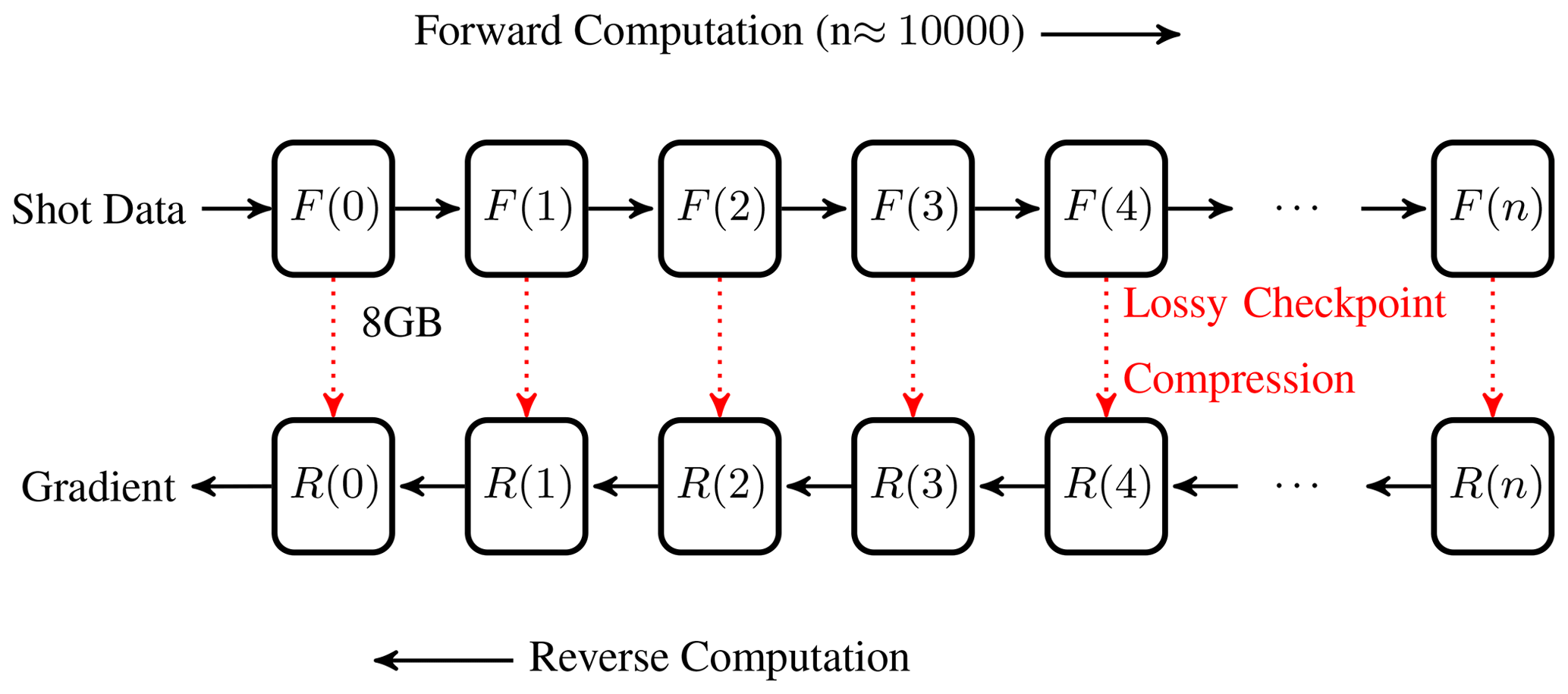
Figure 1 An illustration of the approach presented in this paper. Checkpoints are compressed using lossy compression to combine lossy compression and the checkpoint-recompute strategies.

Many algorithmic optimizations and approximations are commonly applied to reduce the computational load from the numbers calculated in Table 1. These optimizations could either reduce the number of operations or the amount of memory required. In this paper, we shall focus on the high memory footprint of this problem. One standard approach is to save the field at only the boundaries and reconstruct the rest of the field from the boundaries to reduce the memory footprint. However, the applicability of this method is limited to time-reversible PDEs. In this work, we use the isotropic acoustic equation as the example. Although this equation is time-reversible, many other variations used in practice are not. For this reason, we do not discuss this method in this paper.

A commonly used method to deal with the problem of this large memory footprint is domain decomposition over messaging–passing interface (MPI), where the computational domain is split into subdomains over multiple compute nodes to use their memory. The efficacy of this method depends on the ability to hide the MPI communication overhead behind the computations within the subdomain. For effective communication–computation overlap, the subdomains should be big enough that the computations within the subdomain take at least as long as the MPI communication. This places a lower bound on subdomain size (and hence peak memory consumption per MPI rank) that is a function of the network interconnect – this lower bound might be too large for slow interconnects, e.g., on cloud systems.

Some iterative frequency domain methods, e.g., Knibbe et al. (2014), can alleviate the memory limit but are not competitive with time domain methods in the total time to solution.

Hybrid methods that combine time domain methods, as well as frequency domain methods, have also been tried (Witte et al., 2019). However, this approach can be challenging because the application code must decide the user's discrete set of frequencies to achieve a target accuracy.

In the following subsections, we discuss three techniques that are commonly used to alleviate this memory pressure – namely numerical approximations, checkpointing, and data compression. The common element in these techniques is that all three solve the problem of high memory requirement by increasing the operational intensity of the computation – doing more computations per byte transferred from memory. With the gap between memory and computational speeds growing wider as we move into the exaFLOP era, we expect to use such techniques more moving forward.

1.2 Approximate methods

There has been some recent work on alternate floating-point representations (Chatelain et al., 2019), although we are not aware of this technique being applied to FWI. Within FWI, many approximate methods exist, including on-the-fly Fourier transforms (Witte et al., 2019). However, it is not clear whether this method can provide fine-tuned bounds on the solution's accuracy. In contrast, other completely frequency-domain-based formulations can provide clearer bounds (van Leeuwen and Herrmann, 2014); however, as previously discussed, this comes at the cost of a much higher computational complexity. In this paper, we restrict ourselves to time domain approaches only.

Another approximation commonly applied to reduce the memory pressure in FWI in the time domain is subsampling. Here, the time step rate of the gradient computation (See Eq. 4) is decoupled from the time step rate of the adjoint wave field computation, with one gradient time step for every n adjoint steps. This reduces the memory footprint by a factor of n, since only one in n values of the forward wave field needs to be stored. The Nyquist theorem is commonly cited as the justification for this sort of subsampling. However, the Nyquist theorem only provides a lower bound on the error – it is unclear whether an upper bound on the error has been established for this method. Although more thorough empirical measurements of the errors induced in subsampling have been done before (Louboutin and Herrmann, 2015), we do a brief empirical study in Sect. 4.7 as a baseline to compare the error with our method.

1.3 Checkpointing

Instead of storing the wave field at every time step during the forward computation, it is possible to store it at a subset of the time steps only. During the following computation that proceeds in a reverse order to calculate the gradient, if the forward wave field is required at a time step that was not stored, it can be recovered by restarting the forward computation from the last available time step. This is commonly known as checkpointing. Algorithms have been developed to define the optimal checkpointing schedule involving forward, store, backward, load, and recompute events under different assumptions (Griewank and Walther, 2000; Wang et al., 2009; Aupy and Herrmann, 2017). This technique has also been applied to FWI-like computations (Symes, 2007).

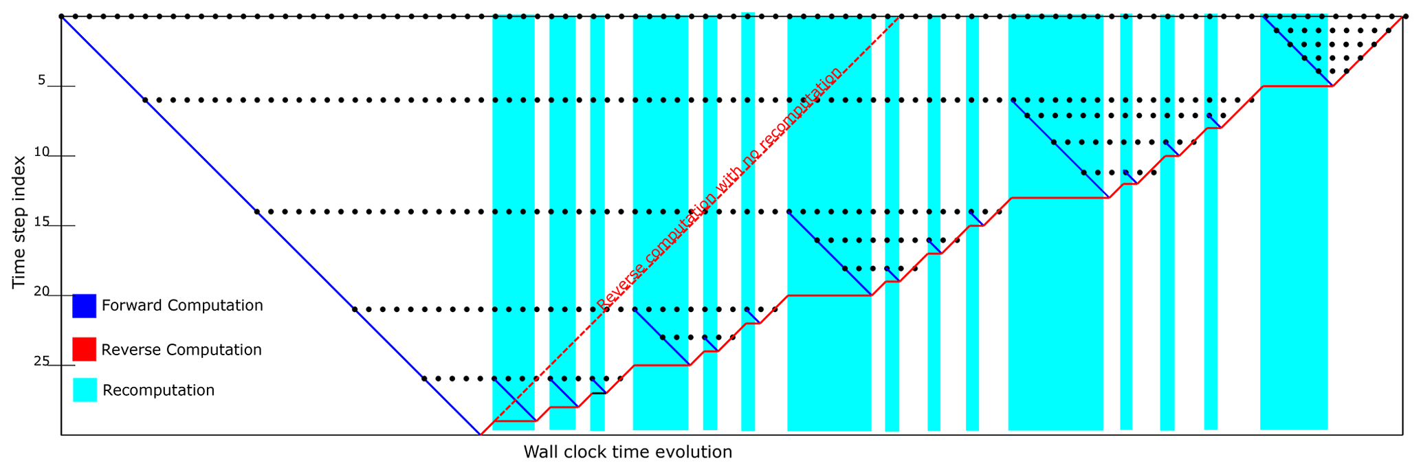
Figure 2 Schematic of the checkpointing strategy. Wall-clock time is on the horizontal axis, while the vertical axis represents simulation time. The blue line represents forward computation. The dotted red line represents how the reverse computation would have proceeded after the forward computation if there had there been enough memory to store all the necessary checkpoints. Checkpoints are shown as black dots. The reverse computation under the checkpointing strategy is shown as the solid red line. It can be seen that the reverse computation proceeds only where the results of the forward computation are available. When not available, the forward computation is restarted from the last available checkpoint to recompute the results of the forward – shown here as the blue-shaded regions.

In previous work, we introduced the open-source software pyRevolve, a Python module that can automatically manage the checkpointing strategies under different scenarios with minimal modification to the computation code (Kukreja et al., 2018). For this work, we extended pyRevolve to integrate lossy compression. For details on the computational implementation of lossy checkpoint compression, as well as a comparison of different compression algorithms based on their compression as well as overheads, please refer to our previous publication (Kukreja et al., 2019a).

The most significant advantage of checkpointing is that the numerical result remains unchanged by applying this technique. Note that we will shortly combine this technique with lossy compression, which might introduce an error, but checkpointing alone is expected to maintain bitwise equivalence. Another advantage is that the increase in run time incurred by the recomputation is predictable.

1.4 Data compression

Compression or bit-rate reduction is a concept originally from signal processing. It involves representing information in fewer bits than the original representation. Since there is usually some computation required to go from one representation to another, compression can be seen as a memory–compute tradeoff.

Perhaps the most commonly known and used compression algorithm is ZLib (from GZip) (Deutsch and Gailly, 1996). ZLib is a lossless compression algorithm, i.e., the data recovered after compressing and decompressing are an exact replica of the original data before compression. Although ZLib is targeted at text data, which are one-dimensional and often have predictable repetition, other lossless compression algorithms are designed for other kinds of data. One example is FPZIP (Lindstrom and Administration, 2017), which is a lossless compression algorithm for multidimensional floating-point data.

For floating-point data, another possibility is lossy compression, where the compressed and decompressed data are not exactly the same as the original data but a close approximation. The precision of this approximation is often set by the user of the compression algorithm. Two popular algorithms in this class are SZ (Di and Cappello, 2016) and ZFP (Lindstrom, 2014).

Compression has often been used to reduce the memory footprint of adjoint computations in the past, including Weiser and Götschel (2012); Boehm et al. (2016); Marin et al. (2016). However, all of these studies use hand-rolled compression algorithms specific to the corresponding task – Weiser and Götschel (2012) focuses on parabolic equations, Boehm et al. (2016) focuses on wave propagation like us, and Marin et al. (2016) focuses on fluid flow. All three use their own lossy compression algorithm to compress the entire time history and look at checkpointing as an alternative to lossy compression. In this paper we use a more general floating-point compression algorithm – ZFP. Since this compressor has been extensively used and studied across different domains and has implementations for various hardware platforms – this lends a sense of trust in this compressor, increasing the relevance of our work. None of the previously mentioned studies combine compression and checkpointing as we do here.

Cyr et al. (2015) perform numerical experiments to study the propagation of errors through an adjoint problem using compression methods like principal component analysis (PCA). However, they do not consider the combination of checkpointing and compression in a single strategy.

Floating-point representation can be seen as a compressed representation that is not entirely precise. However, the errors introduced by the floating-point representation are already accounted for in the standard numerical analysis as noise. The errors introduced by ZFP's compression of fields are more subtle since the compression loss is pattern sensitive. Hence, we tackle it empirically here.

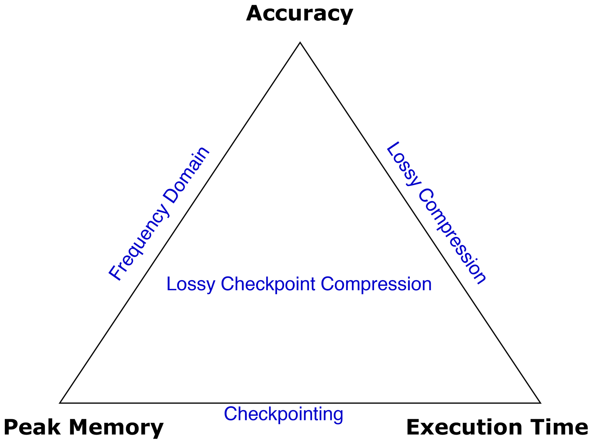
Figure 3 Schematic of the three-way tradeoff presented in this paper. With the use of checkpointing, it was possible to trade off memory and execution time (the horizontal line). With the use of compression alone, it was possible to trade off memory and accuracy. The combined approach presented in this work provides a novel three-way tradeoff.

1.5 Contributions

The last few sections discussed some existing methods that allow tradeoffs that are useful in solving FWI on limited resources. While checkpointing allows a tradeoff between computational time and memory, compression allows a tradeoff between memory and accuracy. This work combines these three approaches into one three-way tradeoff.

In previous work (Kukreja et al., 2019a), we have shown that it is possible to accelerate generic adjoint-based computations (of which FWI is a subset), by using lossy compression on the checkpoints. For a given checkpoint absolute error tolerance (atol), compression may or may not accelerate the computation. The performance model from Kukreja et al. (2019a) helps us answer this question a priori, i.e., without running any computations.

In this work, we evaluate this method on the specific problem of FWI, specifically the solver convergence and accuracy.

To this end, we conduct an empirical study of the following factors:

1. the propagation of errors when starting from a lossy checkpoint,

2. the effect of checkpoint errors on the gradient computation,

3. the effect of decimation and subsampling on the gradient computation,

4. the accumulation of errors through the stacking of multiple shots,

5. the effect of the lossy gradient on the convergence of FWI.

The rest of the paper is organized as follows. Section 2 gives an overview of FWI. This is followed by a description of our experimental setup in Sect. 3. Next, Sect. 4 presents the results, followed by a discussion in Sect. 5. Finally, we present our conclusions and future work.

2 Full waveform inversion

FWI is designed to numerically simulate a seismic survey experiment and invert for the Earth parameters that best explain the observations. In the physical experiment, a ship sends an acoustic impulse through the water by triggering an explosion. The waves created as a result of this impulse travel through the water into the Earth's subsurface. The reflections and turning components of these waves are recorded by an array of receivers being dragged in tow by the ship. A recording of one signal sent and the corresponding signals received at each of the receiver locations is called a shot. A single experiment typically consists of 10 000 shots.

Having recorded this collection of data (d_obs), the next step is the numerical simulation. This starts with a wave equation. Many equations exist that can describe the propagation of a sound wave through a medium – the choice is usually a tradeoff between accuracy and computational complexity. We mention here the simplest such equation, which describes isotropic acoustic wave propagation:

$$\begin{array}{}\text{(1)}& m\left(x\right){\displaystyle \frac{{\partial }^{\mathrm{2}}u(t,x)}{\partial t^{\mathrm{2}}}}-{\mathrm{\nabla }}^{\mathrm{2}}u(t,x)=q_{\mathrm{s}}(t,x),\end{array}$$

where $m\left(x\right)=\frac{\mathrm{1}}{c^{\mathrm{2}}\left(x\right)}$ is the squared slowness, c(x) the spatially dependent speed of sound, u(t,x) is the pressure wave field, ∇²u(t,x) denotes the Laplacian of the wave field, and q_s(t,x) is a source term. Solving Eq. (1) for a given m and q_s can give us the simulated signal that would be received at the receivers. Specifically, the simulated data can be written as follows:

$$\begin{array}{}\text{(2)}& d_{\mathrm{sim}}=P_{\mathrm{r}}u=P_{\mathrm{r}}A(m{)}^{-\mathrm{1}}{P}_{\mathrm{s}}^{\top }{q}_{\mathrm{s}},\end{array}$$

where P_r is the measurement operator that restricts the full wave field to the receivers locations, A(m) is the linear operator that is the discretization of the operator corresponding to Eq. (1), and P_s is a linear operator that injects a localized source (q_s) into the computational grid.

Using this, it is possible to set up an optimization problem that aims to find the value of m that minimizes the difference between the simulated signal (d_sim) and the observed signal (d_obs):

$$\begin{array}{}\text{(3)}& \underset{m}{\mathrm{argmin}}{\mathrm{\Phi }}_{\mathrm{s}}\left(m\right)={\displaystyle \frac{\mathrm{1}}{\mathrm{2}}}{∥d_{\mathrm{sim}}-d_{\mathrm{obs}}∥}_{\mathrm{2}}^{\mathrm{2}}.\end{array}$$

This objective function Φ_s(m) can be minimized using a gradient descent method. The gradient can be computed as follows:

$$\begin{array}{}\text{(4)}& \mathrm{\nabla }{\mathrm{\Phi }}_{\mathrm{s}}\left(m\right)=\sum _{t=\mathrm{1}}^{n_t}u\left[t\right]v_{\mathrm{tt}}\left[t\right]=J^T\mathit{\delta }d,\end{array}$$

where u[t] is the wave field from Eq. (1) and v_tt[t] is the second derivative of the adjoint field (Tarantola, 1984). The adjoint field is computed by solving an adjoint equation backwards in time. The appropriate adjoint equation is a result of the choice of the forward equation. In this example, we chose the acoustic isotropic equation (Eq. 1), which is self-adjoint. However, it is not always trivial to derive the adjoint equation corresponding to a chosen forward equation (Hückelheim et al., 2019). This adjoint computation can only be started once the forward computation (i.e., the one involving Eq. 1) is complete. Commonly, this is done by storing the intermediate values of u during the forward computation, then starting the adjoint computation to get values of v, and using that and the previously calculated u to directly calculate ∇Φ_s(m) in the same loop. This need to store the intermediate values of u during the forward computation is the source of the high memory footprint of this method.

The computation described in the previous paragraph is for a single shot and must be repeated for every shot, and the final gradient is calculated by averaging the gradients calculated for the individual shots. This is repeated for every iteration of the minimization. This entire minimization problem is one step of a multi-grid method that starts by inverting only the low-frequency components on a coarse grid and adding higher-frequency components that require finer grids over successive inversions.

3 Experimental setup

3.1 Reference problem

We use Devito (Kukreja et al., 2016; Luporini et al., 2020b; Louboutin et al., 2019) to build an acoustic wave propagation experiment. The velocity model was initialized using the SEG overthrust model. This velocity model was then smoothed using a Gaussian function to simulate a starting guess for a complete FWI problem. The original domain was surrounded by a 40-point deep-absorbing boundary layer. This led to a total of $\mathrm{287}\times \mathrm{881}\times \mathrm{881}$ grid points. This was run for 4000 ms with a step of 1.75 ms, making 2286 time steps. The spatial domain was discretized on a grid with a grid spacing of 20 m, and the discretization was of the 16th order in space and the second order in time. We used 80 shots for our experiments with the sources placed along the x dimension, spaced equally, and located just under the water surface. The shots were generated by modeling a Ricker source of peak frequency 8 Hz.

The FWI experiments were run on Azure's Kubernetes Service, using the framework described in Zhang et al. (2021). Each cloud worker instance processed only one shot at a time, although there were 20 cloud worker instances running in parallel. The processing of each shot started by reading shot data, previously written to Azure Blob Storage, straight to the cloud worker instance. This was followed by a long gradient computation step (approximately 10 min). Due to this, we posit that file input–output did not play a role in the experiments discussed here.

Following the method outlined in Peters et al. (2019), we avoid inverse crime by generating the shots using a variation of Eq. (1) that includes density, while using Eq. (1) for inversion. The gradient was scaled by dividing by the norm of the original gradient in the first iteration. This problem solved in double precision is what we shall refer to as the reference problem in the rest of this paper. Note that this reference solution itself has many sources of error, including floating-point arithmetic and the discretization itself.

As can be seen in Sect. 2, there is only one wave field in the isotropic acoustic equation, the pressure field, which is called u in the equations. This is the field we compress in all of the experiments. The lossy-compression algorithm accepts a value for absolute error tolerance (atol) a priori and is expected to respect this tolerance during the compression–decompression cycle. We verify this as part of our experiments. Note that the word absolute is used here from the point of view of the compression – we are choosing an absolute value of error tolerance. The absolute value of acceptable error will probably change for waves of different amplitudes. Peak signal-to-noise ratio can be used to calibrate the results here across different pressure amplitudes.

3.2 Error metrics

Let $\mathbf{F}(\mathbf{i},\mathbf{j},\mathbf{k})$ be the original field (i.e., before any compression or loss) and $\mathbf{G}(\mathbf{i},\mathbf{j},\mathbf{k})$ be the field recovered after lossy compression of $\mathbf{F}(\mathbf{i},\mathbf{j},\mathbf{k})$, followed by decompression. We report errors using the following metrics.

PSNR

: peak signal-to-noise ratio, we define this as follows:

$$\begin{array}{}\text{(5)}& \text{PSNR (dB)}=\mathrm{10}{\text{log}}_{\mathrm{10}}{\displaystyle \frac{R^{\mathrm{2}}}{\text{MSE}}},\end{array}$$

where R is the range of values in the field to be compressed, and MSE is the mean squared error between the reference and the lossy field. More precisely,

$$\begin{array}{}\text{(6)}& \text{MSE}={\displaystyle \frac{\mathrm{1}}{\mathrm{mnp}}}\sum _{\mathit{k}=\mathrm{0}}^p\sum _{\mathit{j}=\mathrm{0}}^n\sum _{\mathit{i}=\mathrm{0}}^m\left[\mathbf{F}\right(\mathbf{i},\mathbf{j},\mathbf{k})-\mathbf{G}(\mathbf{i},\mathbf{j},\mathbf{k}){]}^{\mathrm{2}},\end{array}$$

and $R=\text{max}\left(\mathbf{F}\right(\mathbf{i},\mathbf{j},\mathbf{k}\left)\right)-\text{min}\left(\mathbf{F}\right(\mathbf{i},\mathbf{j},\mathbf{k}\left)\right)$.

Angle

: we treat $\mathbf{F}(\mathbf{i},\mathbf{j},\mathbf{k})$ and $\mathbf{G}(\mathbf{i},\mathbf{j},\mathbf{k})$ as vectors and calculate the angle between them as follows:

$$\begin{array}{}\text{(7)}& cos\mathit{\theta }={\displaystyle \frac{\overrightarrow{\mathit{F}}\cdot \overrightarrow{\mathit{G}}}{∥\overrightarrow{\mathit{F}}∥\cdot ∥\overrightarrow{\mathit{G}}∥}}.\end{array}$$

Error norms

: we also report some errors by defining the error vector $\mathit{E}\mathbf{(}\mathit{i}\mathbf{,}\mathit{j}\mathbf{,}\mathit{k}\mathbf{)}$ as $\mathbf{F}(\mathbf{i},\mathbf{j},\mathbf{k})-\mathbf{G}(\mathbf{i},\mathbf{j},\mathbf{k})$ and reporting L₂ and L_∞ norms of this vector.

4 Results

4.1 Evolution of compressibility

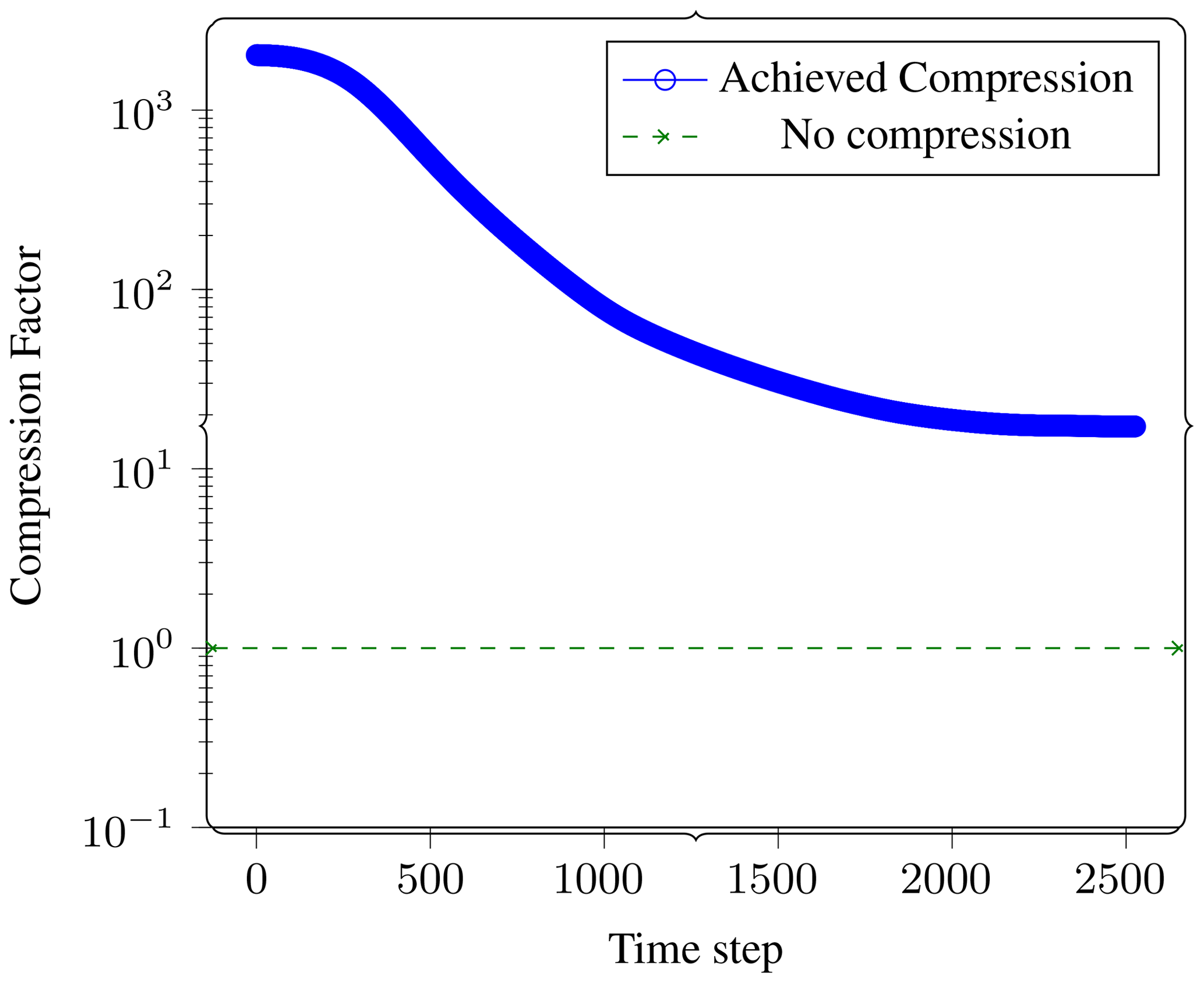
Figure 4 Evolution of compressibility through the simulation. We compressed every time step of the reference problem using an absolute error tolerance (atol) setting of 10⁻⁴. The compression factor achieved is plotted here as a function of the time step number. Higher is more compression. The dotted line represents no compression. We can see that the first few time steps are compressible to 1000x since they are mostly zeros. The achievable compression factor drops as the wave propagates through the domain and seems to stabilize to 20x towards the end. We pick the last time step as the reference field for further experiments.

To understand the evolution of compressibility, we compress every time step of the reference problem using the same compression setting and report on the achieved compression factor as a function of the time step.

This is shown in Fig. 4. It can be seen that in the beginning the field is highly compressible since it consists of mostly zeros. The compressibility is worst towards the end of the simulation when the wave has reached most of the domain.

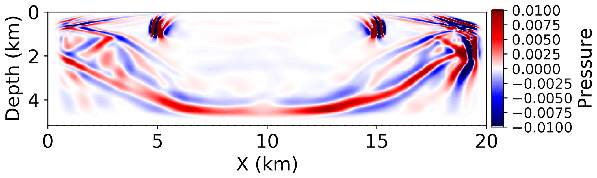
Figure 5 A 2D slice of the last time step of the reference solution. The wave has spread through most of the domain. The values in this figure have been thresholded to ±0.01 for easy visualization. For pressure amplitudes, see Fig. 6.

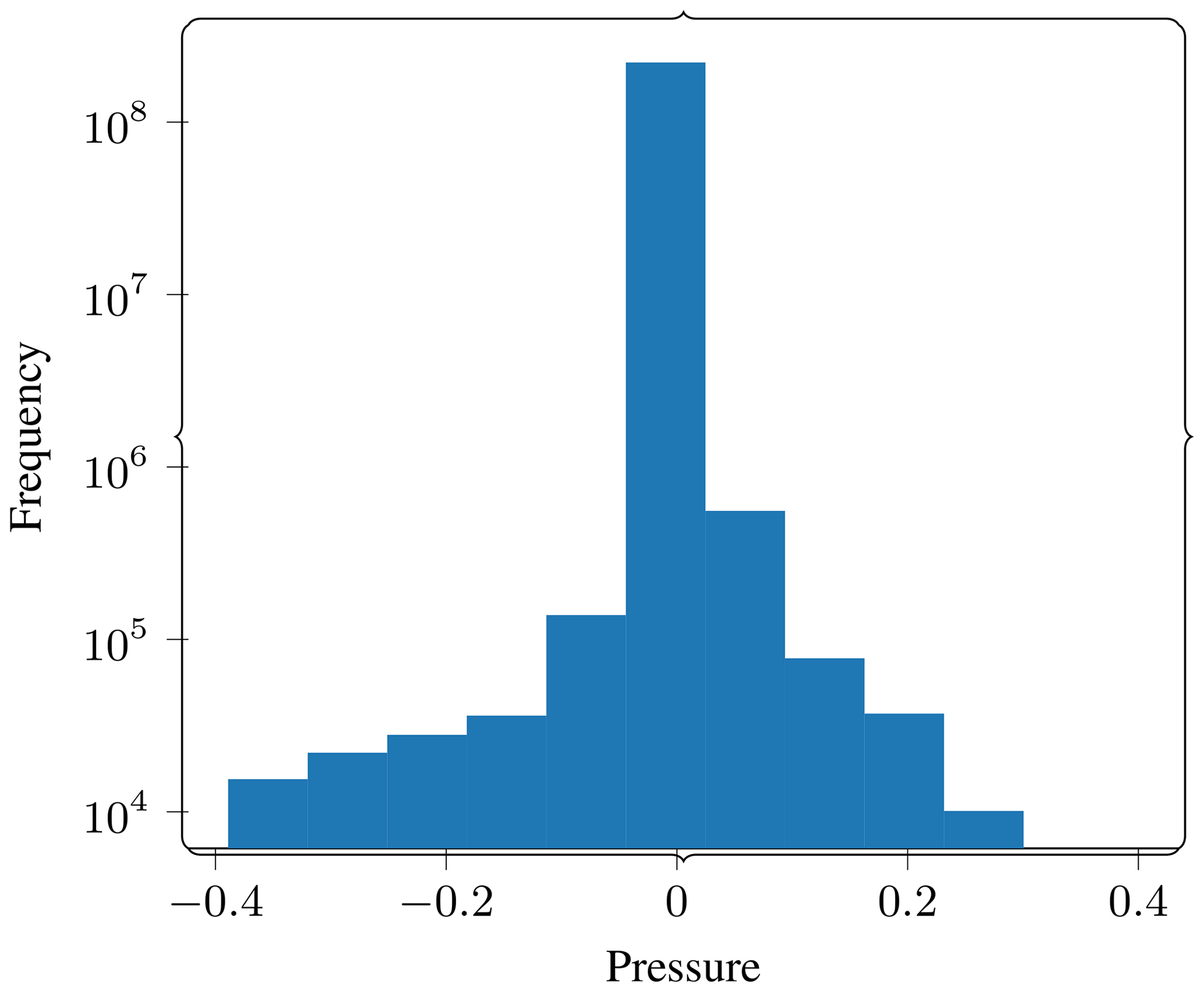
Therefore, we pick the last time step as the reference for further experiments. A 2D cross section of this snapshot is shown in Fig. 5. Figure 6 shows a histogram of pressure values in order to give us an idea of the absolute pressure amplitude present in the wave field being compressed. This plot can be used to give context to the absolute error tolerances in the rest of the results.

Figure 6 A histogram of pressure values in the wave field shown in Fig. 5. These values can be used to give context to the absolute error tolerances used in the rest of the experiments.

4.2 Direct compression

To understand the direct effects of compression, we compressed the reference wave field using different absolute tolerance (atol) settings and observed the errors incurred as a function of atol. The error is a tensor of the same shape as the original field and results from subtracting the reference field and the lossy field. Figure 7 shows the peak signal-to-noise ratio achieved for each atol setting. Figure A1 in Appendix A shows some additional norms for this error tensor.

Figure 7 Direct compression. We compress the wave field at the last time step of the reference solution using different absolute error tolerance (atol) settings and report the peak signal-to-noise ratio (PSNR) achieved. Higher PSNR is lower error. The PSNR is very high for low atol and drops predictably as atol is increased. See Fig. A1 for more metrics on this comparison.

4.3 Forward propagation

Next, we ran the simulation for 550 steps and compressed the field's final state after this time. We then compress and decompress this through the lossy compression algorithm, getting two checkpoints – a reference checkpoint and a lossy checkpoint. We then restarted the simulation from step 550, comparing the progression of the simulation restarted from the lossy checkpoint vs. a reference simulation that was started from the original checkpoint. We run this test for another 250 time steps.

Figure 8 shows the evolution of the PSNR between wave fields at corresponding time steps as a function of the number of time steps evolved. There is a slight initial drop followed by essentially constant values for the 250 time steps propagated. This tells us that the numerical method is robust to the error induced by lossy compression and that the error does not appear to be forcing the system to a different solution.

Figure 8 Forward propagation. We stop the simulation after about 500 time steps. We then compress the state of the wave field at this point using atol $={\mathrm{10}}^{-\mathrm{6}}$. We then continue the simulation from the lossy checkpoint and compare it with the reference version. Here we show the error as PSNR. In these plots, higher is better, whereas lower implies more error. The PSNR dropped slightly over the first few time steps and then remains essentially constant after.

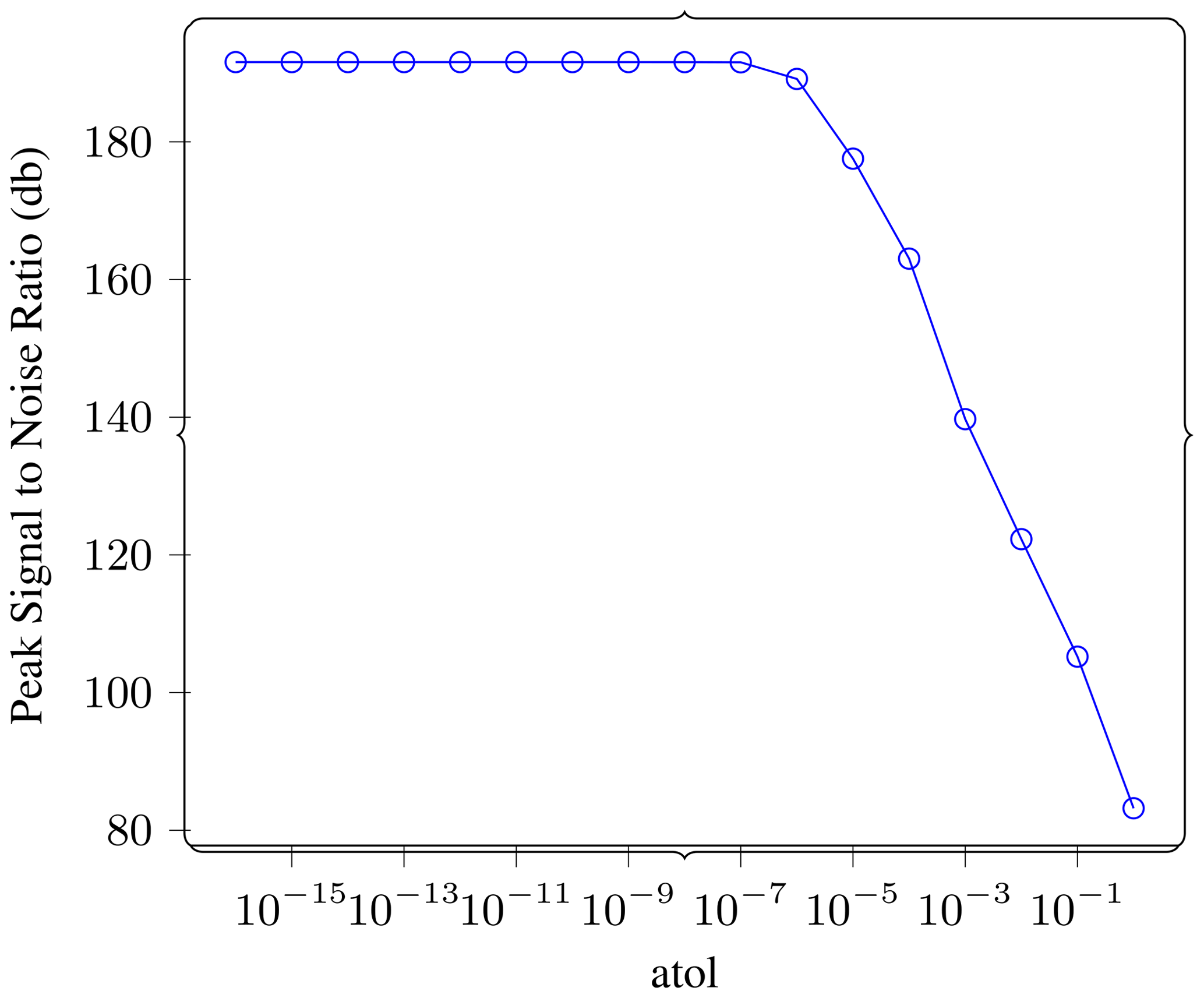
Figure 9 Gradient computation. In this experiment we carry out the full forward–reverse computation to get a gradient for a single shot while compressing the checkpoints at different atol settings. This plot shows the PSNR of reference vs. lossy gradient as a function of atol on the lossy checkpoints. We can see that the PSNR remains unchanged until about atol $={\mathrm{10}}^{-\mathrm{6}}$, and that it is very high even at very high values of atol.

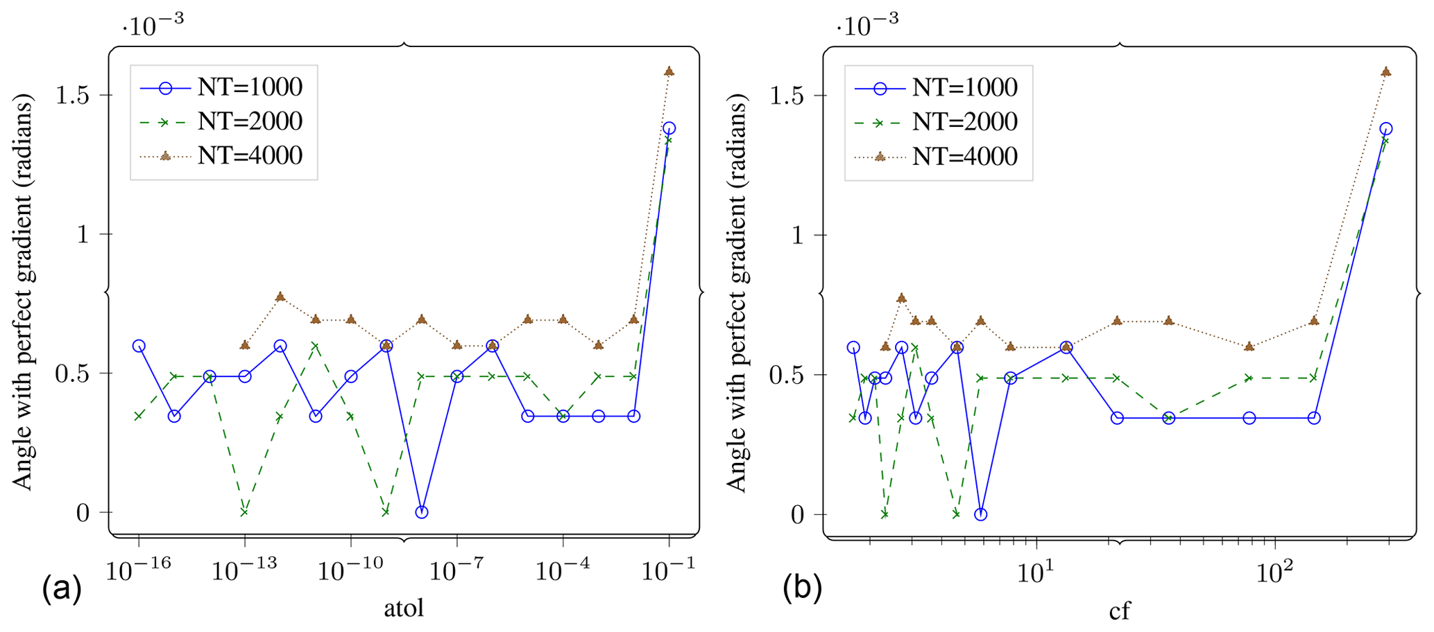
Figure 10 Gradient computation. Angle between the lossy gradient vector and the reference gradient vector (in radians) vs. atol (a) and vs. compression factor (b). If the lossy gradient vector was pointing in a significantly different direction compared to the reference gradient, we could expect to see that on this plot. The angles are quite small. The number of time steps do not affect the result by much. The results are also resilient to increasing atol up to 10⁻². Compression factors of over 100x do not seem to significantly distort the results either.

Figure 11 Gradient error. L_∞ (a) and L₂ (b) norms of the gradient error as a function of the achieved compression factor (CF). It can be seen that error is negligible in the range of CF up to 16. Figure 19 repeats a part of these results to aid comparison with the subsampling strategy.

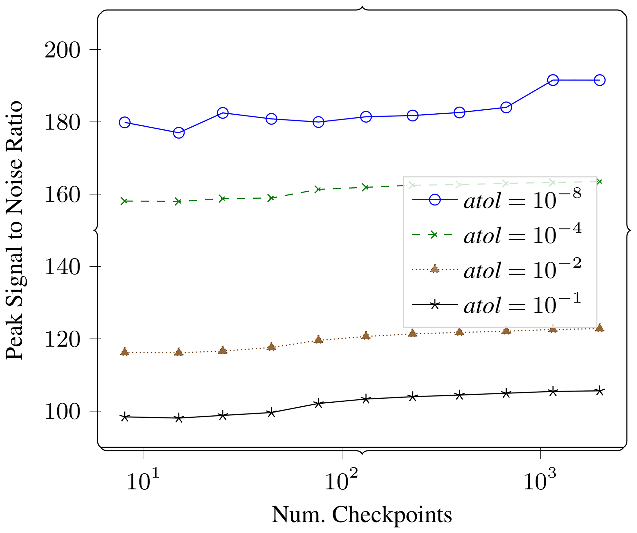
Figure 12 Gradient error. In this plot we measure the effect of varying number of checkpoints on the error in the gradient. We report PSNR of lossy vs. reference gradient as a function of number of checkpoints for four different compression settings.

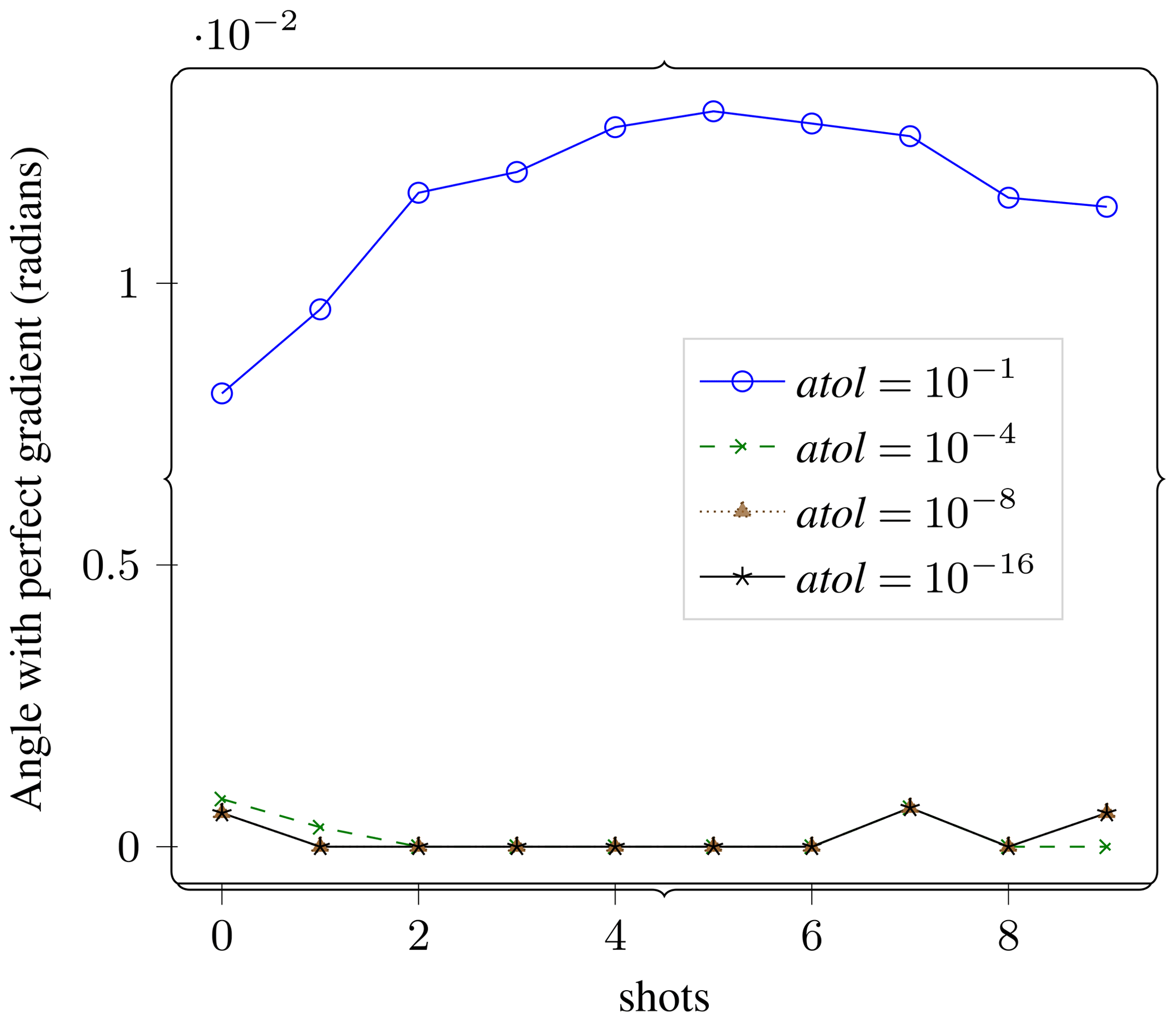
Figure 13 Shot stacking. The gradient is first computed for each individual shot and then added up for all the shots. In this experiment we measure the propagation of errors through this step. This plot shows that while errors do have the potential to accumulate through the step, as can be seen from the curve for $atol={\mathrm{10}}^{-\mathrm{1}}$ for compression settings that are useful otherwise, the errors do not accumulate significantly.

Figure 14 True model used for FWI.

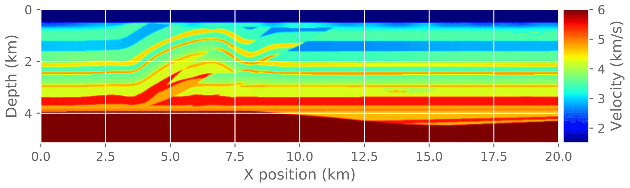
Figure 15 Reference solution for the complete FWI problem. This is the solution after running reference FWI for 30 iterations.

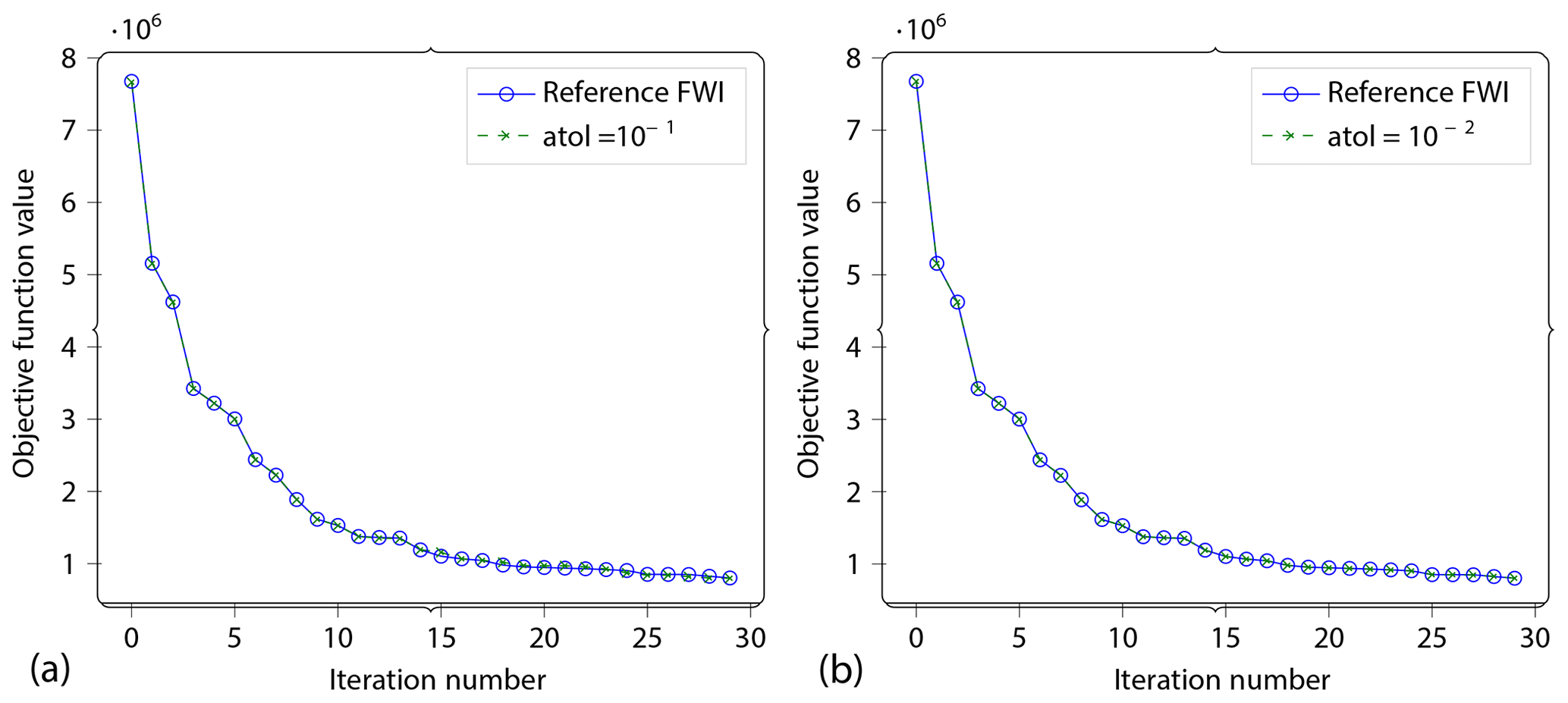
Figure 16 Convergence. As the last experiment, we run complete FWI to convergence (up to max 30 iterations). Here we show the convergence profiles for $atol={\mathrm{10}}^{-\mathrm{1}}$ (a) and $atol={\mathrm{10}}^{-\mathrm{2}}$ (b) vs. the reference problem. The reference curve is so closely followed by the lossy curve that the reference curve is hidden behind it.

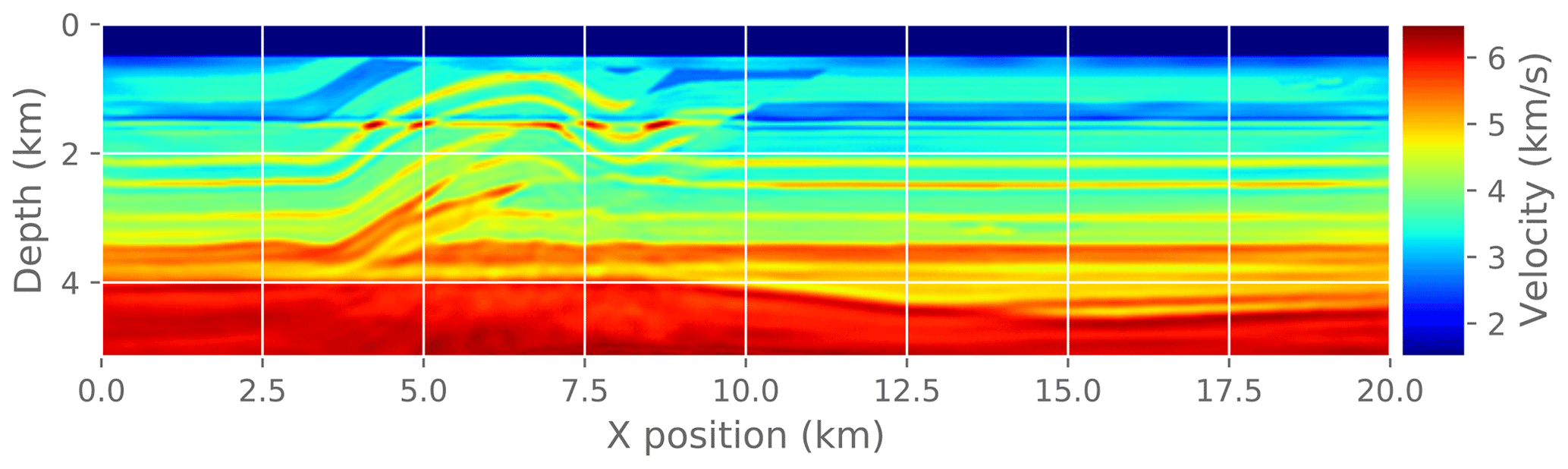
Figure 17 The final image after running FWI $atol={\mathrm{10}}^{-\mathrm{1}}$. It is visually indistinguishable from the reference solution in Fig. 15.

Figure 18 Final image after running FWI $atol={\mathrm{10}}^{-\mathrm{2}}$. It is visually indistinguishable from the reference solution in Fig. 15.

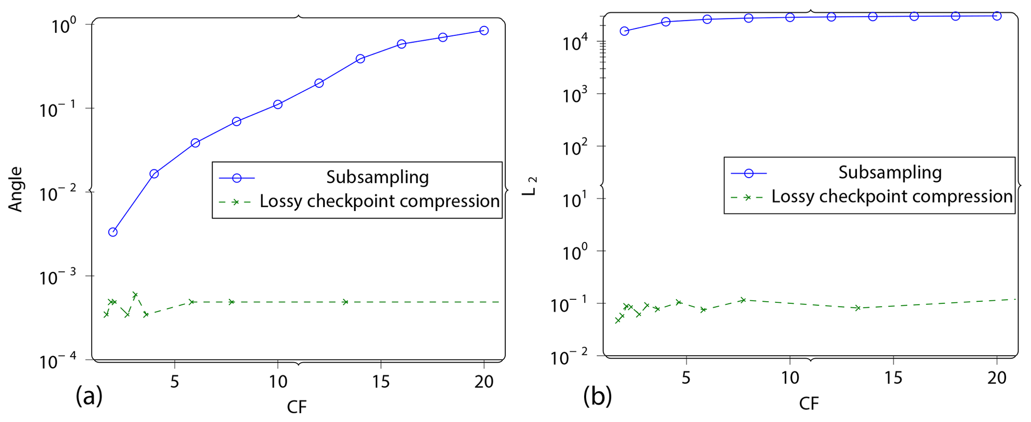
Figure 19 Subsampling. We set up an experiment with subsampling as a baseline for comparison. Subsampling is when the gradient computation is carried at a lower time step than the simulation itself. This requires less data to be carried over from the forward to the reverse computation at the cost of solution accuracy, and thus it is comparable to lossy checkpoint compression. This plot shows the angle between the lossy gradient and the reference gradient vs. the compression factor CF (a) and L₂ norm of gradient error vs. the compression factor CF (b) for this experiment. Compare this to the errors in Fig. 11 that apply for lossy checkpoint compression.

4.4 Gradient computation

In this experiment, we do the complete gradient computation, as shown in Fig. 1, once for the reference problem and for a few different lossy settings. We measured the error in the gradient computation as a function of atol using the same compression settings for all checkpoints.

In Fig. 9, we report the error between the reference gradient and the lossy gradient as PSNR (see Sect. 3.2 for definition). The PSNR remains unchanged until an atol of 10⁻⁶, and even at its lowest it is at a very high value of 80.

In Fig. 10, we look at the same experiment but through a different metric. Here we report the angle between the reference gradient vector and the lossy gradient vector. We see that the error remains constant at a very small value of $\mathrm{5}\times {\mathrm{10}}^{-\mathrm{4}}$ radian up to $atol={\mathrm{10}}^{-\mathrm{2}}$. This same plot also shows that the number of time steps do not appear to change the error by much (for a constant number of checkpoints).

In Fig. 11, we report the error as L_∞ and L₂ norms with respect to achieved compression factor. This makes it easier to compare with the subsampling strategy presented later (see Fig. 19).

We also repeated the gradient computation for different number of checkpoints. Fewer checkpoints would apply lossy compression at fewer points in the calculation, while the amount of recomputation would be higher. More checkpoints would require less recomputation but would apply lossy compression at more points during the calculation. Figure 12 shows the results of this experiment. We see that the PSNR is largely dependent on the value of atol and does not change much when the number of checkpoints is changed by 2 orders of magnitude.

It can be seen from the plots that the errors induced in the checkpoint compression do not propagate significantly until the gradient computation step. In fact, the atol compression setting does not affect the error in the gradient computation until a cutoff point. It is likely that the cross-correlation step in the gradient computation is acting as an error-correcting step since the adjoint computation continues at the same precision as before – the only errors introduced are in the values from the forward computation used in the cross-correlation step (the dotted arrows in Fig. 1).

4.5 Stacking

After gradient computation on a single shot, the next step in FWI is the accumulation of the gradients for individual shots by averaging them into a single gradient. We call this stacking. In this experiment we studied the accumulation of errors through this stacking process. Figure 13 shows the error in the gradient computation (compared to a similarly processed reference problem) as a function of the number of shots.

This plot shows us that the errors across the different shots are not adding up and that the cumulative error is not growing with the number of shots, except for the compression setting of $atol={\mathrm{10}}^{-\mathrm{1}}$, which is chosen as an example of unreasonably high compression.

4.6 Convergence

Finally, we measure the effect of an approximate gradient on the convergence of the FWI problem. In practice, FWI is run for only a few iterations at a time as a fine-tuning step interspersed with other imaging steps. Here we run a fixed number of FWI iterations (30) to make it easier to compare different experiments. To make this a practical test problem, we extract a 2D slice from the original 3D velocity model and run a 2D FWI instead of a 3D FWI. We compare the convergence trajectory with the reference problem and report. For reference, Fig. 14 shows the known true velocity model for this problem. Figure 15 shows the final velocity model after running a reference FWI for 30 iterations. Figure 17 shows the final velocity model after running FWI with compression enabled at different atol settings (also for 30 iterations).

Figure 16 shows the convergence trajectory – the objective function value as a function of the iteration number. We show this convergence trajectory for two different compression settings. It can be seen that the compressed version does indeed follow a very similar trajectory to the original problem.

4.7 Subsampling

As a comparison baseline, we also use subsampling to reduce the memory footprint as a separate experiment and track the errors. Subsampling is another method to reduce the memory footprint of FWI that is often used in industry. The method is set up so that the forward and adjoint computations continue at the same time step as the reference problem. However, the gradient computation is now not done at the same rate – it is reduced by a factor f. We plot results for varying f.

Figure 19 shows some error metrics as a function of the compression factor f.

Comparing Fig. 19 with 11, it can be seen that the proposed method produces significantly smaller errors for similar compression factors.

5 Discussion

The results indicate that significant lossy compression can be applied to the checkpoints before the solution is adversely affected. This is an interesting result because, while it is common to see approximate methods leading to approximate solutions, this is not what we see in our results: the solution error does not change much for large compression error. This being an empirical study, we can only speculate on the reasons for this. We know that in the proposed method, the adjoint computation is not affected at all – the only effect is in the wave field carried over from the forward computation to the gradient computation step. Since the gradient computation is a cross-correlation, we only expect correlated signals to grow in magnitude in the gradient calculation and when gradients are stacked. The optimization steps are likely to be error-correcting processes as well, since even with an approximate gradient ($atol>{\mathrm{10}}^{-\mathrm{4}}$) the convergence trajectory and the final results do not appear to change much – indicating that the errors in the gradient might be canceling out over successive iterations. There is even the possibility that these errors in the gradient act as a regularization (Tao et al., 2019). This is likely since we know from Diffenderfer et al. (2019) that ZFP's errors are likely to smoothen the field being compressed. We also know from Tao et al. (2019) that ZFP's errors are likely to be (close to) normally distributed with zero mean, which reinforces the idea that this is likely to act as a regularizer. We only tried this with the ZFP compression algorithm in this work. ZFP being a generic floating-point compression algorithm, is likely to be more broadly applicable than application-specific compressors. This makes it more broadly useful for Devito, which was the domain-specific language (DSL) that provided the context for this work. Some clear choices for the next compressors to try would be SZ (Di and Cappello, 2016), which is also a generic floating-point compression library, and the application-specific compressors from Weiser and Götschel (2012); Boehm et al. (2016); Marin et al. (2016). A different compression algorithm would change the following parameters:

• the error distribution,

• the compression and decompression times, and

• the achieved compression factors.

Based on the experiments from Tao et al. (2019), we would expect the errors in SZ to be (nearly) uniformly distributed with a zero mean. It would be interesting to see the effect this new distribution has on the method we describe here. If a new compressor can achieve higher compression factors than ZFP (for illustration) with less compression and decompression time than ZFP, then it will clearly speed up the application relative to ZFP. In reality, the relationship is likely to be more complex, and the performance model from Kukreja et al. (2019a) helps compare the performance of various compressors on this problem without running the full problem. The number of checkpoints has some effect on the error – more checkpoints incur less error for the same compression setting – as would be expected. Since we showed the benefits of compression for inversion, the expected speedup does not depend on the medium that varies between iterations from extremely smooth to very heterogeneous. While we focused on acoustic waves in this work for simplicity, different physics should not impact the compression factor due to the strong similarity between the solutions of different wave equations. However, different physics might require more fields in the solution – increasing the memory requirements, while also increasing the computational requirements. Whether this increase favors compression or recomputation more depends on the operational intensity of the specific wave equation kernel. The choice of misfit function is also not expected to impact our results since the wave field does not depend on the misfit function. A more thorough study will, however, be necessary to generalize our results to other problem domains such as computational fluid dynamics that involve drastically different solutions.

Our method accepts an acceptable error tolerance as input for every gradient evaluation. We expect this to be provided as part of an adaptive optimization scheme that requires approximate gradients in the first few iterations of the optimization and progressively more accurate gradients as the solution approaches the optimum. Such a scheme was previously described in Blanchet et al. (2019). Implementing such an adaptive optimizer and using it in practice is ongoing work.

6 Conclusions and future work

In the preceding sections, we have shown that by using lossy compression, high-compression factors can be achieved without significantly impacting the convergence or final solution of the inversion solver. This is a very promising result for the use of lossy compression in FWI. The use of compression in large computations like this is especially important in the exascale era, where the gap between computing and memory speed is increasingly large. Compression can reduce the strain on the memory bandwidth by trading it off for extra computation. This is especially useful since modern CPUs are hard to saturate with low operational intensity (OI) computations.

In future work, we would like to study the interaction between compression errors and the velocity model for which FWI is being solved, as well as the source frequency. We would also like to compare multiple lossy compression algorithms, e.g., SZ.

Appendix A: Additional results

A1 Direct compression

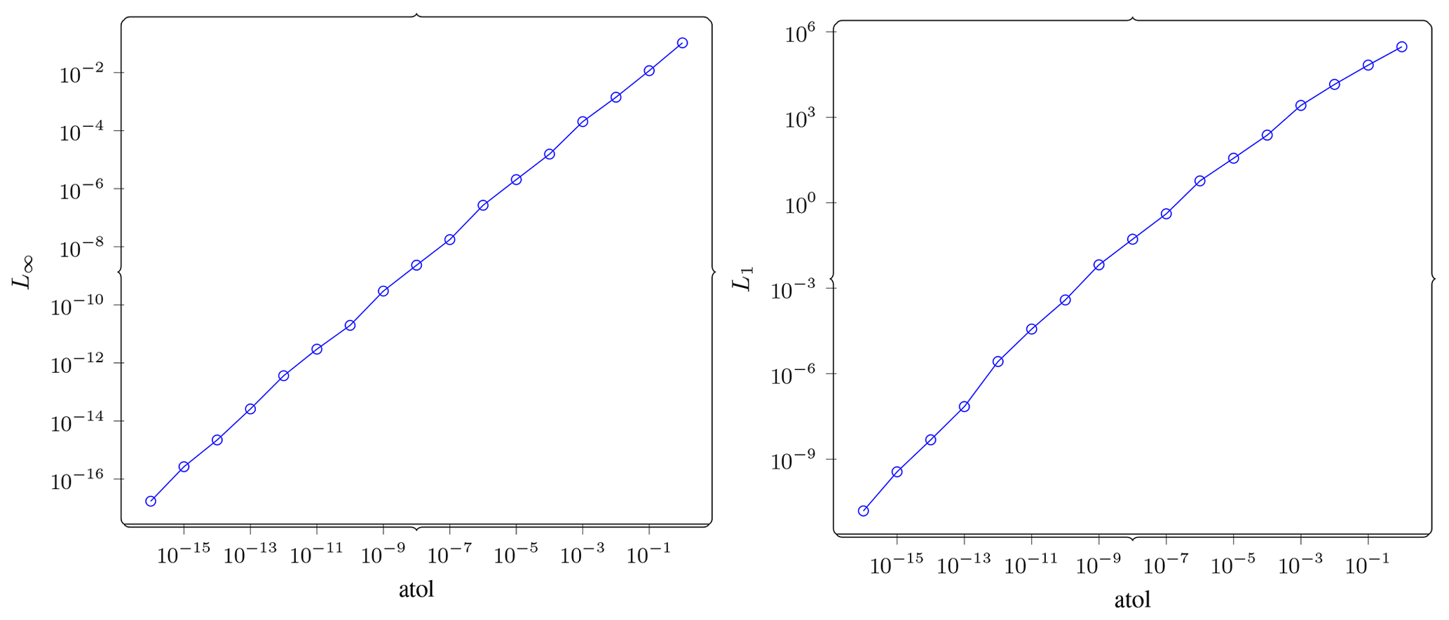
Figure A1 Direct compression. On the left, L_∞ norm of error vs. atol is shown. This plot verifies that ZFP respects the tolerance we set. On the right, L₁ norm of error vs. atol is shown. From the difference in magnitude between the L_∞ plot and this one, we can see how the error is spread across the domain.

A2 Gradient computation

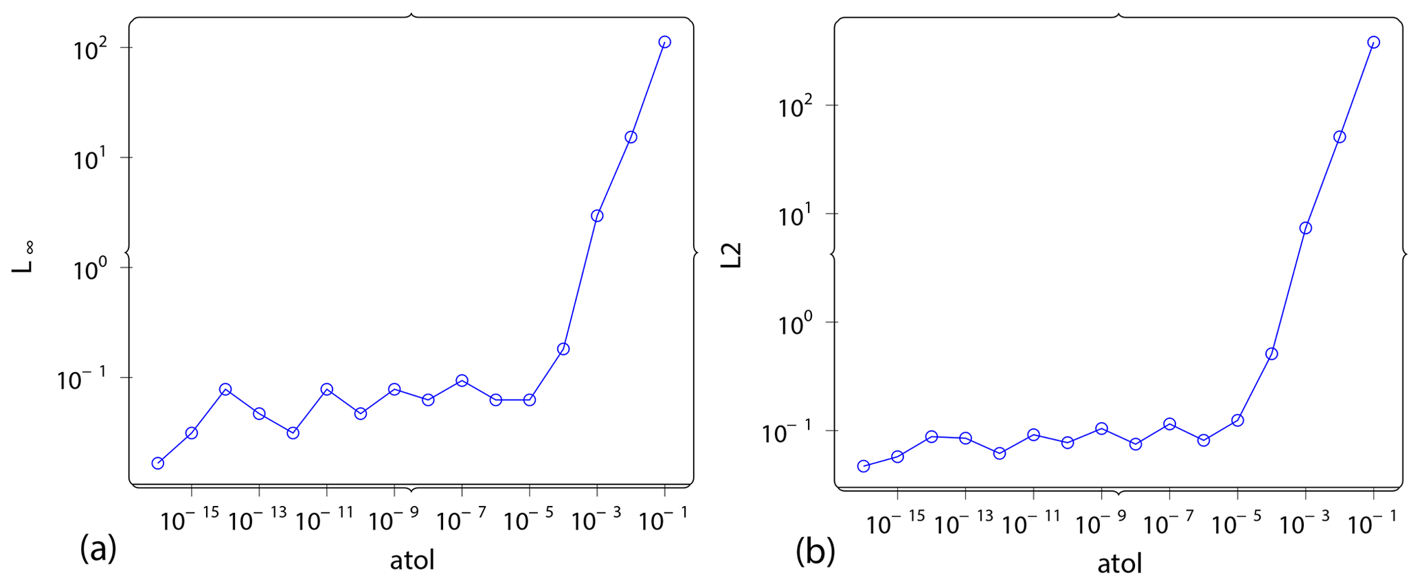
Figure A2 Gradient computation. L_∞ norm of gradient error vs. atol (a) and L₂ norm of gradient error vs. atol are shown. It can be seen that the error stays almost constant and very low up to a threshold value of 10⁻⁴.