the Creative Commons Attribution 4.0 License.
the Creative Commons Attribution 4.0 License.
 | 20 Apr 2022
Development of an open-source regional data assimilation system in PEcAn v. 1.7.2: application to carbon cycle reanalysis across the contiguous US using SIPNET
Bailey D. Morrison
Ann Raiho
Shawn P. Serbin
Katie Zarada
Luke Dramko
Michael Dietze
The ability to monitor, understand, and predict the dynamics of the terrestrial carbon cycle requires the capacity to robustly and coherently synthesize multiple streams of information that each provide partial information about different pools and fluxes. In this study, we introduce a new terrestrial carbon cycle data assimilation system, built on the PEcAn model–data eco-informatics system, and its application for the development of a proof-of-concept carbon “reanalysis” product that harmonizes carbon pools (leaf, wood, soil) and fluxes (GPP, Ra, Rh, NEE) across the contiguous United States from 1986–2019. We first calibrated this system against plant trait and flux tower net ecosystem exchange (NEE) using a novel emulated hierarchical Bayesian approach. Next, we extended the Tobit–Wishart ensemble filter (TWEnF) state data assimilation (SDA) framework, a generalization of the common ensemble Kalman filter which accounts for censored data and provides a fully Bayesian estimate of model process error, to a regional-scale system with a calibrated localization. Combined with additional workflows for propagating parameter, initial condition, and driver uncertainty, this represents the most complete and robust uncertainty accounting available for terrestrial carbon models. Our initial reanalysis was run on an irregular grid of ∼ 500 points selected using a stratified sampling method to efficiently capture environmental heterogeneity. Remotely sensed observations of aboveground biomass (Landsat LandTrendr) and leaf area index (LAI) (MODIS MOD15) were sequentially assimilated into the SIPNET model. Reanalysis soil carbon, which was indirectly constrained based on modeled covariances, showed general agreement with SoilGrids, an independent soil carbon data product. Reanalysis NEE, which was constrained based on posterior ensemble weights, also showed good agreement with eddy flux tower NEE and reduced root mean square error (RMSE) compared to the calibrated forecast. Ultimately, PEcAn's new open-source regional data assimilation framework provides a scalable workflow for harmonizing multiple data constraints and providing a uniform synthetic platform for carbon monitoring, reporting, and verification (MRV) as well as accelerating terrestrial carbon cycle research.
- Article
(4243 KB) - Full-text XML
- BibTeX
- EndNote


Accurate assessment of both biogenic carbon stocks and exchanges between the biosphere and atmosphere is crucial for a more complete carbon monitoring, reporting, and verification (MRV) framework, as well as understanding climate–carbon feedbacks. However, quantifying different components of the carbon cycle to identify whether different regions and/or landscapes are C sinks or sources has been a major challenge for Earth scientists (Williams et al., 2005) as the sink strength of the terrestrial biosphere is more variable than the ocean (Battle et al., 2000). For this reason, investigating the current and future state of the terrestrial carbon cycle has gained considerable scientific attention.
Substantial time and energy have been devoted to developing terrestrial carbon data products aimed at MRV and improving our understanding of the carbon cycle at broader spatial scales. Some of these products are based on upscaled field measurements that interpolate between observations, such as forest biomass maps based on inventory plots (Pan et al., 2011), soil carbon maps based on soil cores (Mikhailova et al., 2016), and carbon flux maps based on eddy covariance (Xiao et al., 2014). Other products are based on calibrating remote sensing measurements against in situ data, such as leaf area index (Liu et al., 2018) and aboveground biomass (Myneni et al., 2001), or quantifying properties that correlate strongly with carbon stocks or changes in those stocks, such as land use and land cover (Schillaci et al., 2017) or disturbance (Liu et al., 2011). These data products describe particular processes or features of the terrestrial carbon cycle at various spatial scales and have been essential to improving our understating of plant and soil processes. However, each of these products reflects a single pool or flux and is thus only showing us part of the picture about the terrestrial carbon cycle. It is a highly challenging task to combine this wealth of observational information into a coherent and comprehensible view of the carbon cycle and ensure consistency between the available data products (Cavallaro et al., 2018). Furthermore, many parts of the carbon cycle are hard to observe at large scales, and our understanding of the processes that connect different pools and fluxes is often limited to smaller numbers of intensively studied sites rather than large-scale monitoring. Therefore, often times, the full potential of these datasets, as well as their combination, is not fully exploited (Montzka et al., 2012).
An alternative to the piecewise understanding provided by derived data products is to use process-based terrestrial biosphere models (TBMs) to quantify and understand carbon cycle dynamics holistically. The strength of TBMs lies in their ability to represent the carbon cycle in an internally consistent manner that conserves mass and captures our current understanding of physical, chemical, and biological processes. However, their weakness comes from the many uncertainties that are present in such models, most of which are not formally accounted for in current applications (Raiho et al., 2020; Dietze, 2017). Most existing terrestrial models have been developed using deterministic strategies in which uncertainties associated with model drivers, model parameters, and initial conditions are ignored (Peylin et al., 2016). In addition, these models can have considerable amounts of process error, which arises from a combination of inherent stochasticity (e.g., disturbance, mortality, dispersal), heterogeneity in ecosystem processes, and structural uncertainties that reflect our imperfect knowledge about how to best represent system processes (Williams et al., 2005). The result is models that are not well-constrained and are highly prone to producing large errors (Scholze et al., 2017). Because of this, it is critical that we properly propagate uncertainties into TBM predictions and continuously confront those predictions with observational data to reduce the uncertainties around TBM predictions (Scholze et al., 2017).
Rather than relying on models or data alone, data assimilation techniques offer a method for combining their strengths and addressing their weaknesses. Data assimilation (DA) refers to a robust mathematical framework for constraining model predictions with observational data within which the intellectual motivation is to construct an integrated view of a system. Data assimilation is fundamentally a data-driven exercise focused on the synthesis of information across different data streams and provides a statistical framework for linking data sources with different temporal and spatial resolutions to generate a composite data product that contains significantly more information than the individual data sources (Dietze, 2017). Unlike statistical data fusion approaches, data assimilation can also link together data about different pools and fluxes by leveraging the process understanding that is embedded in models, which in turn is often linked to intensively studied sites. In a data assimilation system, we can even exploit non-carbon observations to constrain the carbon cycle indirectly through the relations implemented in the process model (Scholze et al., 2017). At the same time, data assimilation systems act to continually constrain model uncertainties and continually pull models back to what actually occurred rather than the many possible futures models may envision. As such, DA is distinctly different from, and potentially more powerful than, either forward simulations of calibrated models or derived data products that transform observations through statistical models alone.
When run as a hindcast, a frequent goal of data assimilation is to produce a “reanalysis” product. The goal of a reanalysis product is to provide a synthetic, harmonized best estimate of past pools and fluxes across space and time. Reanalysis products are popular in many parts of the Earth system sciences, such as harmonized climate reanalysis products generated by rerunning weather models constrained by historical observations. Reanalysis products are studied directly to better understand system properties, processes, and spatiotemporal variability as well as to serve as inputs to other models and analyses. However, despite their clear potential to improve MRV and scientific understanding, there has been little effort to develop large-scale reanalysis products for the terrestrial carbon cycle. Our goal in this paper is to demonstrate an initial “proof of concept” for a national-scale terrestrial carbon reanalysis that spans the contiguous US over a multi-decadal period (1986–2019) during which remotely sensed data constraints are available at a large scale.
Among data assimilation approaches to generate a carbon cycle reanalysis, sequential data assimilation (SDA), in which new observations are assimilated iteratively through time, holds particular promise for combining a suite of datasets available on the terrestrial carbon cycle. There are a number of studies examining different approaches and applications of DA systems in carbon cycle assessment (Arakida et al., 2017). However, most studies are limited by their spatial extent (e.g., single site) (Albergel et al., 2010; Kivi et al., 2022), the set of uncertainties that are propagated (e.g., missing some combination of process, driver, or parameter uncertainty), the number of data constraints, demonstrated ability to support multiple models, or the assumptions of their statistical model. Many modeling studies have relied on an incomplete accounting of model uncertainty. For example, some data assimilation studies have relied solely on meteorological driver uncertainty to generate ensemble spread (Fox et al., 2018; Kumar et al., 2019; Ling et al., 2019) or spin-ups to represent initial condition uncertainty, and frequently, these studies lack parameter uncertainty (Albergel et al., 2010; Bacour et al., 2015) or model–data process error (Ling et al., 2019; Kumar et al., 2019; Demarty et al., 2007; Arakida et al., 2017). Data assimilation might be routinely done at a single site, but as the number of sites increases new opportunities and challenges arise (e.g., how to leverage spatiotemporal covariance between the sites) that make developing a regional system capable of overcoming these limitations challenging. Among studies focused on the use of SDA for terrestrial carbon analysis, Viskari et al. (2020) continuously updated the Yasso15 model's state variables to improve soil organic carbon estimates. Similarly, Viskari et al. (2015) used tower and satellite observations of phenological state to improve seasonal carbon fluxes in the ED2 model. Fox et al. (2018) assimilated leaf area index (LAI) and biomass into the CLM4.5 model using an ensemble adjustment Kalman filter and showed that model carbon forecasts in central New Mexico were improved on monthly and longer timescales. Raczka et al. (2021) also used the CLM5-DART platform to assimilate satellite-based estimates of aboveground biomass and LAI into the CLM5.0 model. They found a reduction in both photosynthesis and respiration fluxes, mainly because their adjusted simulation significantly reduced the aboveground biomass and leaf area. Schürmann et al. (2016) introduced the Max Planck Institute Carbon Cycle Data Assimilation System (MPI-CCDAS) built around the JSBACH model. They used globally distributed fraction of absorbed photosynthetically active radiation (FAPAR) observations and atmospheric CO2 to simulate phenology and net land carbon balance. In another study, (Chen et al., 2008) developed a joint parameter and state data assimilation method called SEnKF that not only dramatically reduced the uncertainty in state variables, but also accounted for the temporal evolution of model parameters. In a site-level study Gao et al. (2011) used an ensemble Kalman filter (EnKF) in a data assimilation scheme to forecast the carbon cycle. Overall, these studies confirm that EnKF can effectively assimilate multiple datasets into a TBM.
Here, we build on a decade of work on uncertainty propagation and analysis within the PEcAn model–data informatics system (LeBauer et al., 2013; Fer et al., 2020) to generate the most complete and robust uncertainty accounting available to date (Raiho et al., 2020). At a high level, we use an ensemble-based approach to propagate data-driven uncertainty in model drivers, initial conditions, and parameters, with parameter distributions derived from an across-site hierarchical Bayesian calibration against AmeriFlux NEE and plant trait data. In addition, within the SDA we rely on the new Tobit–Wishart ensemble filter (TWEnF) to dynamically update and propagate a fully Bayesian estimate of the entire process error covariance matrix. The TWEnF also relaxes the strong Gaussian assumption behind most data assimilation methods, allowing for both zero truncation (no negative values) and zero inflation (more zeros than expected by the Gaussian), both of which are common features of ecological data.
In this study, we focus on scaling up our previous site-level SDA (Raiho et al., 2020) to a national-scale terrestrial carbon reanalysis. In doing so we developed, tested, and calibrated a spatial localization algorithm for our covariance matrix (Petrie and Dance, 2010), estimating a 500 km distance threshold beyond which covariances are set to zero to avoid spurious correlations. This system can run on an irregular spatial grid that uses cluster analyses to optimally distribute points in a multivariate environmental space (i.e., temperature, precipitation, elevation, estimated actual evapotranspiration – AET, climatic water deficit) that reduces computational costs and better captures complex terrain than a regular grid. We also extended the TWEnF to calculate and save the spatiotemporally varying posterior weights of each ensemble member, which allows us to infer sub-daily fluxes (e.g., GPP, NEE) across the simulation region even though our assimilation was run at an annual timescale. Having developed this system, we then report on our initial proof-of-concept reanalysis, which was constrained by MODIS leaf area index (LAI) and LandTrendr aboveground biomass (AGB). Finally, we perform an initial validation against AmeriFlux NEE and SoilGrids soil organic carbon.
2.1 PEcAn platform and SIPNET model
We developed our regional state data assimilation framework within an ecological model–data informatics system, the Predictive Ecosystem Analyzer (PEcAn) v. 1.7.2, and under a module named assim.sequential. PEcAn is a toolbox that provides a unified format and workflow for processing inputs and outputs, running models, and performing analyses for a wide range of ecological models. PEcAn tools include sensitivity and uncertainty analysis, benchmarking, and parameter and state data assimilation (LeBauer et al., 2013; Fer et al., 2018; Raiho et al., 2020; Fer et al., 2020). PEcAn also provides a robust procedure for sampling and propagating uncertainties by generating ensembles across initial conditions, model parameters, and model drivers (soil and meteorological forcing). All methodological developments and tool improvements introduced in this paper have been added to PEcAn, which is available at https://doi.org/10.5281/zenodo.5557914 and on GitHub (https://github.com/pecanproject/pecan/, last access: 14 April 2022), as a virtual machine (https://opensource.ncsa.illinois.edu/projects/artifacts.php?key=PECAN, last access: 14 April 2022), or as a series of Docker containers (https://hub.docker.com/u/pecan, last access: 14 April 2022). PEcAn documentation is available through the project web page (https://pecanproject.org, last access: 14 April 2022).
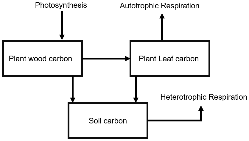
We used the Simplified Photosynthesis and Evapotranspiration model (SIPNET) model (Braswell et al., 2005) within the PEcAn platform v. 1.7.2 as the process model for our regional data assimilation exercise. SIPNET was chosen for this initial proof of concept as it is computationally efficient but provides a non-trivial representation of carbon pools and fluxes. SIPNET represents the carbon cycle as a series of pools and fluxes; it accounts for two vegetation carbon pools (leaf and wood) and a single aggregated soil carbon pool (Fig. 1). To reduce the number of parameters in the SIPNET model, it makes the assumption that carbon stored in the leaves remains constant throughout the growing season, and therefore all fluxes in the carbon cycle (Fig. 1) only affect the plant wood carbon pool. In addition, rather than a complex carbon allocation and phenology model, SIPNET uses a simple time-based function to model the phenology; on a specific day of the year, all leaves appear or fall off in a single time step. The simple representation of the carbon cycle in SIPNET provides the opportunity to fully constrain both model parameters and state variables.
2.2 Model calibration
To efficiently capture variability in vegetation properties across the contiguous US (CONUS), we aggregated National Land Cover Database (NLCD) land cover (Homer et al., 2012) into four plant functional types (PFTs): deciduous forest, evergreen forest, mesic grassland, and arid grassland–shrubland. For deciduous forest we rely on the previous calibration reported by Fer et al. (2021). The same methods were used to calibrate the remaining PFTs against a combination of plant trait data and eddy covariance, as described below.
2.3 Priors and trait meta-analysis
PEcAn takes a fully Bayesian approach to model calibration. Calibration begins with defining prior distributions for 35 parameters for the grass PFT and 32 parameters for the evergreen PFT. These priors were then updated using plant trait data in the BETY-db (LeBauer et al., 2018) by performing a hierarchical Bayesian meta-analysis following the methods described in LeBauer et al. (2013). Trait data for seven parameters (SLA, Amax, leafC, leaf respiration rate, leaf turnover rate, root respiration rate, root turnover rate) were available from 6 to 213 studies for different parameters. Meta-analysis posteriors were then used as informative priors in the subsequent sensitivity analysis and calibration, for which they help ensure the selection of biologically plausible parameter estimates.
2.3.1 Global sensitivity analysis (GSA)
Prior to model calibration, we performed global sensitivity analyses on the SIPNET model parameters at five grassland and five evergreen AmeriFlux sites located across different ecoregions. The aim of this analysis was to reduce the dimensionality of the calibration by identifying the dominant parameters in the model. The informative prior distributions were sampled to generate 500 ensemble members to test the sensitivity of net ecosystem exchange (NEE) to change in each parameter. Runs at each site were done for 15 years using gap-filled eddy flux tower meteorology as model drivers. A linear model between the simulated mean NEE and the sampled parameter values was used to decompose the variability around NEE and estimate the contribution of each parameter. The linear model included the main effect for each parameter as well as its first interactions. Main effects and total sensitivity indices were calculated using the sum of squares (SSQ) as follows (Dokoohaki et al., 2018; Wallach et al., 2019).
Main effect sensitivity indices
Interaction sensitivity indices
Total sensitivity indices
SS1 is the SSQ for the first parameter, SS12 is the SSQ of the interaction between the first and second parameter, and SST is the total SSQ. Based on the results of these analyses, parameters with a contribution of at least 5 % to the total variability of NEE were selected for further investigation and calibration for both conifer and grass PFTs.
2.3.2 Hierarchical parameter data assimilation
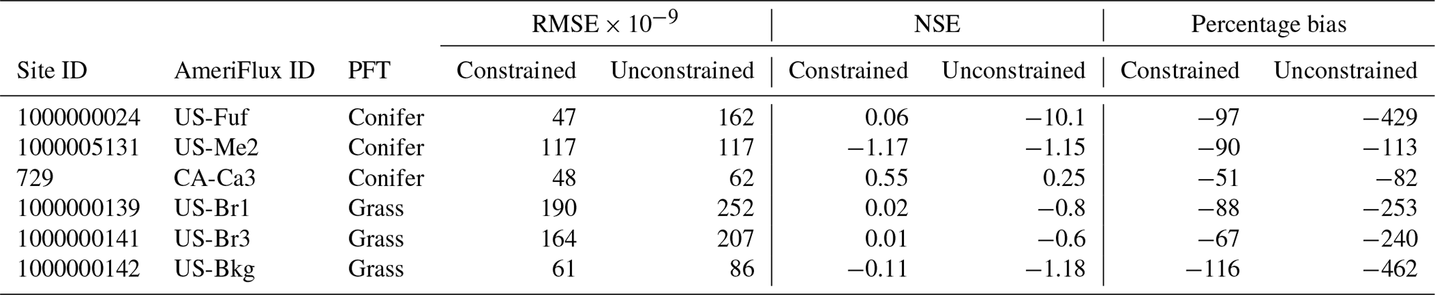
The hierarchical Bayesian parameter data assimilation (HPDA) framework within the PEcAn platform v. 1.7.2 was employed to constrain the most sensitive parameters of the SIPNET model found during the sensitivity analysis. We used HPDA to calibrate model parameters for a combined mesic and semiarid grassland PFT as well as an evergreen forest PFT against NEE observations from six eddy covariance towers (Table 1). In contrast to a site-level model or single-parameter single-site calibration, hierarchical calibration accounts for site-to-site variability while also borrowing strength across sites during the parameter estimation procedure. Consequently, parameters are calibrated for all sites at the same time; generally, the estimated variability across sites identifies site-sensitive parameters or missing processes in models (Fer et al., 2018).
Table 1NSE, RMSE, and percentage bias (estimated as ) estimated before and after parameter assimilation for the grass and coniferous plant functional types across all sites.
Our calibration procedure closely followed Fer et al. (2018) by developing emulators of the likelihood surface at the site level. To develop the emulators, we used an adaptive sampling approach (Fer et al., 2018) to generate an n-dimensional grid over the parameter's space (where n is the number of parameters) and then ran the SIPNET model at the n-dimensional points (e.g., knots) in this parameter set. Model runs were driven by gap-filled tower meteorology and varied in length from site to site depending on available data (Table 1). For each run, we then compared the model's predicted NEE to the observed NEE (30 min time step, no gap filling) and calculated a likelihood score for each knot. Observations were filtered based on u*, and effective sample size was corrected for autocorrelation following Fer et al. (2018). Keeping with previous works (Fer et al., 2018; Reich and Cotter, 2015), we used an asymmetric heteroscedastic Laplace likelihood that accounts for the increase in observation error with the magnitude of the flux and error bias. In our case, these errors are larger in the positive direction (nighttime respiration) than the negative. Site-level emulators were then developed by fitting a Gaussian process (GP) model to the knots to construct a smooth n-dimensional likelihood surface in parameter space. After developing the site-level emulators, the hierarchical calibration was performed by Markov chain Monte Carlo (MCMC). In the hierarchical MCMC, site-level parameters are accepted or rejected using the across-site mean and covariances as priors and using the emulator to predict the likelihood, while across-site mean and covariances are updated through Gibbs sampling (Fer et al., 2018):
where μg and τg represent the global mean parameter vector and the site-to-site covariance matrix, while μs,i represents the i site-level mean parameter vectors for each of n sites. μg and τg were assigned uninformative multivariate normal and Wishart priors, respectively.
Each calibration was run in three iterative rounds with adaptive sampling following Fer et al. (2018), wherein the total number of proposed knots per round was set to p×20 (p represents the number of parameters). In each round we used the posterior mean to propose additional knots in the parts of parameter space needing additional detail, essentially behaving like a nested grid around the posterior mean. Finally, we used the Nash–Sutcliffe model efficiency (NSE) index and root mean square error (RMSE) to evaluate the performance of the model and examine whether the calibration has improved the model's capacity for simulating NEE following HPDA. NSE indicates the goodness of fit of the simulated series against observations (1 indicates a perfect fit).
2.4 Regional site selection
As previously noted, our data assimilation system runs on an irregular grid optimized to efficiently capture environmental variability. For the current proof-of-concept analysis, we identified a total of 517 sites across CONUS by first selecting 46 AmeriFlux sites that would be used to validate the assimilated fluxes, followed by 471 additional potential sites based on a cluster analysis of land cover class (NCLD) and climate variables. The cluster analysis used PRISM 800 m precipitation, maximum and minimum temperature, and elevation, in addition to estimated actual evapotranspiration (AET), climatic water deficit (WD), total surface radiation, rain, and snow. Actual evapotranspiration and water deficit are biologically meaningful parameters that are well correlated with the distribution of vegetation types across multiple spatial scales (Stephenson, 1998). We began by using PRISM 800 m elevation and produced monthly global total irradiance using the GRASS GIS (v7.8) for CONUS (Šúri and Hofierka, 2004). It was assumed that total surface radiation remained consistent throughout the study time period as physical topography and solar distance change little at the decadal timescale. To estimate AET, WD, rain, and snow, we collected 1 by 1∘ historical monthly wind vector data from CCSM4 (Danabasoglu et al., 2020) and estimated 1981–2010 monthly normals using methods reported in Morrison et al. (2019). Using the radiation and wind speed, along with maximum and minimum temperature and precipitation, we derived climatic (not biological) AET and WD, which resulted in monthly climate normals for AET, WD, rain, and snow following methods described in Morrison et al. (2019). Next, a k-means sampling approach was used to determine the number of unique bioenvironmental clusters within each USGS Level 1 ecoregion of CONUS (Omernik, 1987). Maximum and minimum temperature, radiation, AET, WD, rain, snow, and land cover class pixels for a given ecoregion were applied to a k-means algorithm. We performed multiple cluster analyses by increasing the value of k by 1 until at least two clusters were no longer distinct or overlapping one another. The number of unique clusters for an ecoregion was then determined by the maximum k value of distinct or non-overlapping cluster runs.
Lastly, each ecoregion's k value was used as a weight to determine the number of sites per ecoregion, generating the additional 471 randomly sampled sites to run in the SDA workflow, resulting in a total of 517 potential sites. Only sites with acceptable MODIS LAI quality control (QC) values were used in the SDA (000 – best result possible, 001 – good, very usable; Myneni and Park, 2015), resulting in a total of 493 sites to be included in the SDA simulations.
2.5 Sequential state data assimilation
The primary premise of sequential state data assimilation (SDA) methods is that neither models nor observations are perfect, but we can reduce uncertainties by finding a common ground between model simulations and multiple observations. SDA relies on an iterative cycle between forecasts as well as updates and analyses that leverage Bayes' theorem to update the forecast (prior) based on new observations (likelihood) (Fig. 3). For example, for a given site and time, prior to collecting data, model forecasts are the best estimates of the state of a system. The model's forecast can be summarized in terms of a mean vector of state variables, μf, and an error covariance matrix, Pf. Once observations are made, we can update this prior using the newly observed data Y (with associated observation error R) as a component of Bayes’ theorem to calculate a corrected estimate of the state of a system μa and Pa. This update then serves as the initial conditions for further projections in time (Fig. 4) (Dietze, 2017).
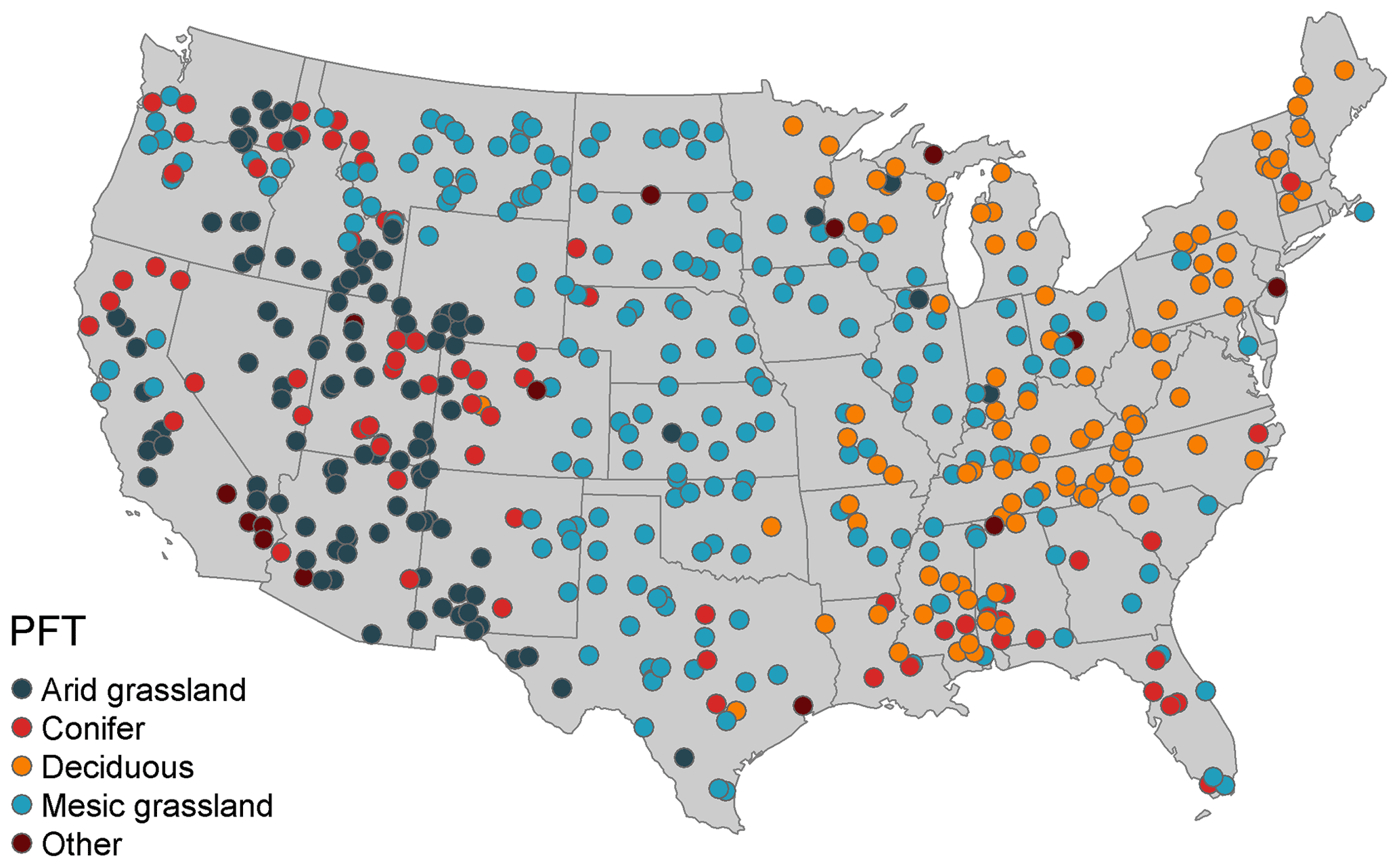
Figure 2Distribution of sites with their corresponding plant functional type across CONUS.
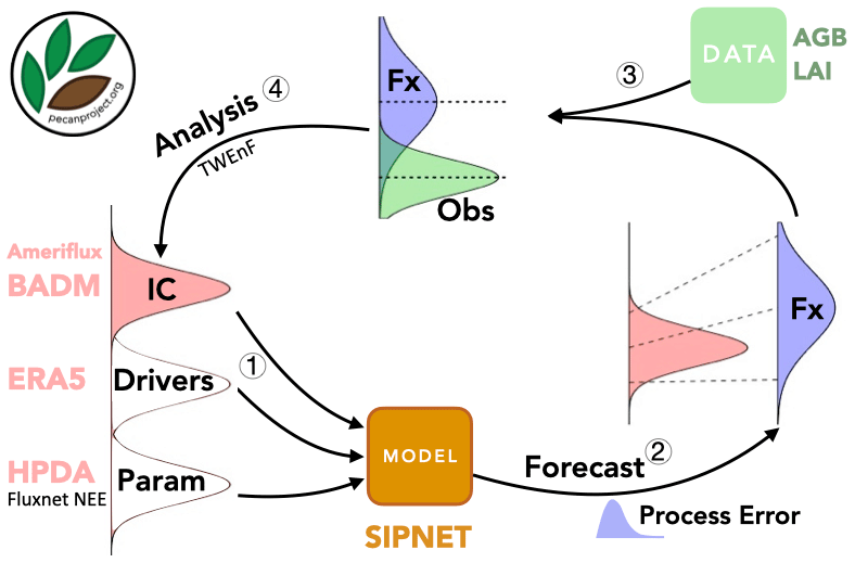
Figure 3PEcAn state data assimilation system: forecast–analysis cycle. Step 1: uncertainty propagation. Step 2: forward forecast. Step 3: data preparation. Step 4: data assimilation.
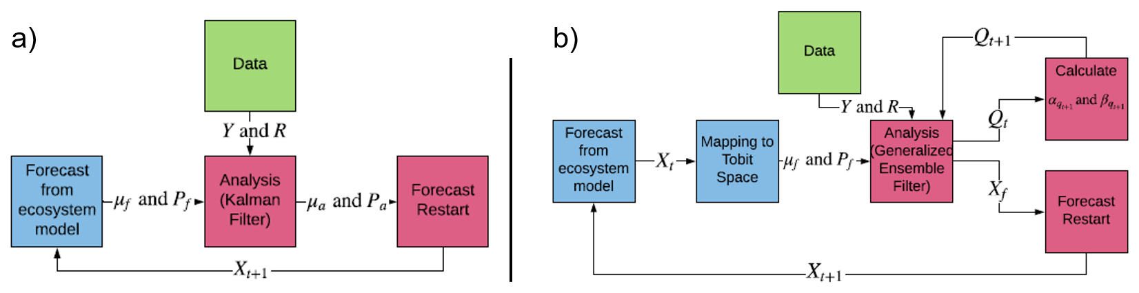
Figure 4(a) Classic ensemble Kalman filter method. (b) Tobit–Wishart ensemble filter. Xf: matrix of model forecasts; μf and Pf: forecast mean and error covariance matrix; μa and Pa: analysis mean and error covariance matrix; Y and R: observation mean and error covariance matrix; Qt model process error. Adopted from Raiho et al. (2020).
Classical data assimilation algorithms such as the ensemble Kalman filter (Evensen, 2009) have been used extensively in weather and ecological forecasting (Raiho et al., 2020; Viskari et al., 2020). However, most of these methods make strong assumptions about the probability distribution of the forecasts and observations and lack the ability to estimate the model process error. For example, the Gaussian assumption in the EnKF algorithm could generate negative soil carbon estimates, and the omission of process error may lead to overconfidence in model forecasts.
To account for censored state variables in our process model, we used the Tobit–Wishart ensemble filter (TWEnF) as described in Raiho et al. (2020) to perform the analysis step within our data assimilation workflow (Fig. 4). The forecast mean, covariance, and the likelihood function were transformed to the Tobit space to account for the left or right censored state variables (e.g., carbon pools cannot be negative). In addition, the prior for our process covariance matrix was assumed to be Wishart, and prior shape parameters were stored and updated at each time step. This gave us the flexibility to not only relax the Gaussian assumption behind the Kalman filter family of data assimilation methods but also to estimate and propagate model process error over the assimilation period.
The TWEnF algorithm presented in Raiho et al. (2020) was expanded in this study to allow for regional data assimilation and multiple types of model process error Q in this study as follows.
Here, xf and X are the model estimates for each ensemble before and after accounting for process error, Q, respectively. αq and βq are the parameters controlling the shape of the model process error Q, and yL represents the lower boundary for the censored observations, which is set to 0 in the current application.
By including the model error covariance estimates from all the sites in one unified model error covariance matrix in the update step, we can take advantage of the covariability between state variables at different sites. As a result, state variables with and without corresponding observations can be updated through their covariance with other variables at other sites. For example, this enables updates to LAI at a site with no direct observations solely based on the covariance estimated with a nearby site with LAI observations. However, the extent to which we allow the sites to update their states could depend on some measure of dissimilarity such as physical or environmental distance between sites (Dietze, 2017). This problem in weather forecasting literature is called the localization problem (Petrie and Dance, 2010). In this study, we set up the localization threshold to 500 km; the covariance between sites was adjusted using an exponential decay function as follows:
where d is the distance matrix between all the sites and ν is the cutoff distance at which covariances will be pushed towards zero. More details on the localization setup can be found in Appendix B.
The new regional-scale generalization of the TWEnF analysis step was implemented in PEcAn v. 1.7.2 and fit in R statistical software (R Core Team, 2013) using the NIMBLE package (de Valpine et al., 2017). At every time step, we ran three chains of MCMC for a total of 100 000 steps and discarded the first 10 000 to account for burn-in. The primary variables of interest were the posterior estimates of μa and Pa and the parameter controlling the covariance and shape of the process error (Q) while assuming the R is known. We reduced the total number of unknown parameters by assuming a shared process error Q among all sites.
Aboveground biomass (AGB) and leaf area index (LAI) estimates were extracted from satellite imagery to act as our observational data to assimilate in the SDA algorithm. Estimates of the annual AGB and the pixel-wise standard deviation (SD) for each study site were collected from Landtrendr (Landsat-based detection of trends in disturbance and recovery) at 30 m resolution from 1983 to 2018 (Kennedy et al., 2018, 2010). LAI, SD, and QC values were collected from MODIS MOD15A2H (Moderate Resolution Imaging Spectroradiometer) at 500 m resolution every 8 d from 2000–2019 for all sample sites (ORNL DAAC, 2018). LAI and SD observations with QC values that were not the “best result” (000) or “good, very usable” (001) were removed from the LAI observation dataset and not used for assimilation (Myneni and Park, 2015). In total, 13 827 AGB observations and 8380 LAI observations passed quality assessment and were included in final data assimilation simulations for 419 sites from 1987–2019. Since the assimilation was run on an annual basis, with the analysis occurring on 15 July, peak LAI was used as our annual LAI metric. Peak LAI was defined as the maximum LAI value within the 95th percentile for a single site and year. Similarly, the SD of peak LAI was defined as the corresponding SD value associated with the peak LAI value for each site and year. Any LAI SD value <0.6 was reassigned a value of 0.6 following Viskari et al. (2015).
At the end of each assimilation cycle, we adjusted the updated state variables by using the ensemble adjustment technique (Anderson et al., 2009) rather than sampling new ensemble members from the analysis posterior in order to maintain the covariance structure between states, drivers, and parameters. The goal of ensemble adjustment is to first shift the ensemble means to have the same mean as the posterior (μa) and also linearly contract ensembles so they also show the same variance as the posterior (Pa) (Anderson et al., 2009).
Our reanalysis was performed by running 20 ensemble members in parallel, each associated with a different set of species parameters, meteorological drivers, and initial conditions. Each assimilation cycle including the total run time for the ensemble simulations (performed in parallel, and each SIPNET simulation took ∼5 s for 1 year) and fitting the GEF model in R software took ≈7.8 h on average. More detailed assessment of SIPNET model run time is presented in Fer et al. (2018). Parameter vectors for each ensemble member were drawn from the HPDA distribution for the across-site mean, μg. The meteorological drivers covered the period from 1986–2019 and were resampled from the 10-ensemble-member ERA5 reanalysis product, which has a 3 h time step and a resolution of 0.5625∘ (62 km). Initial condition distributions were generated by resampling leaf, stem, and soil carbon pool data extracted from the AmeriFlux Biological, Ancillary, Disturbance, and Management (BADM) database on an EPA L1 ecoregion basis.
2.6 Post hoc ensemble weight estimation
To focus our SDA on the model's state variables (carbon pools) and minimize the dimensions of X for more efficient numerical sampling in Eq. (5), we only included the main carbon cycle state variables (aboveground biomass, leaf area index, and soil carbon pool) in the X matrix. Therefore, the model output variables that were not included in the X, such as carbon and water fluxes, were not adjusted during the analysis step itself. Instead, these additional outputs were updated post hoc for each site and time step by estimating the posterior probability of each ensemble member using the following equation:
Equation (10) estimates the likelihood of producing the model simulations given the posterior (analysis) state of the system. Equation (10) provides a relative weight for each ensemble member that varies by year and site. A weighted mean and variance were then estimated for NEE, GPP, autotrophic respiration, and heterotrophic respiration using the estimated weights. These weights are applied not just to the cumulative sum of the fluxes (annual totals) but to the high-frequency time series between analysis time points. This approach was validated by comparing the reanalysis NEE to the AmeriFlux observed NEE at a subset of points.
2.7 Soil carbon validation
To assess our ability to indirectly infer soil carbon from assimilation of LAI and AGB into the SIPNET model, we compared our soil organic carbon (SOC) estimates at all sites against the SoilGrids dataset (Hengl et al., 2017). SoilGrids is an interpolated data product at 250 m resolution produced using machine learning models by taking advantage of global soil profile information and a series of covariate data. We extracted the average soil carbon estimates from the SoilGrids database down to 2 m depth to compare against our reanalysis estimates.
3.1 Global sensitivity analysis and HPDA
The main purpose of the sensitivity analysis was to identify model parameters with a large influence on the behavior of SIPNET output variables such as NEE. The estimated variability presented in Fig. 5 averages the sensitivity of NEE to each parameter across multiple years and different sites, presenting just the parameters that met our 5 % variance criteria. Because NEE is the difference between gross primary productivity (GPP) and total ecosystem respiration we expected that parameters that primarily regulate modeled GPP and respiration would be the most sensitive with respect to NEE. The soil organic matter (SOM) decomposition rate, which controls heterotrophic respiration, was the most sensitivity parameter for both plant functional types. Following SOM respiration rate, photosynthetic optimum temperature (psnTOpt), photosynthetic maximum capacity (Amax), growth respiration factor, and soil respiration Q10 were found to be sensitive in both the conifer and grass PFT. Amax and psnTOpt directly contribute to the GPP calculation, while the growth respiration factor contributes to autotrophic respiration and determines the fraction of GPP that is available for growth. The soil respiration Q10 and psnTOpt both demonstrate SIPNET's high sensitivity to temperature. In addition to shared parameters, the conifer PFT also showed a high sensitivity of GPP to vapor pressure deficit (VPD), which is reflected in the importance of the slope (dVPDSlope) and exponent (dVpdExp) in that equation, and to specific leaf area (SLA), which reflects how much new leaf area a plant can “buy” for an given investment in leaf carbon. The grass PFT, on the other hand, showed a high sensitivity to immedEvapFrac, which is the proportion of incoming precipitation that is intercepted and re-evaporated rather than being allowed to enter the soil and become available for transpiration.
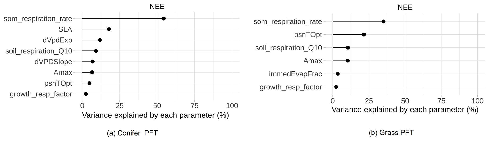
Figure 5Global sensitivity analysis of SIPNET model parameters to NEE prediction for different plant functional types.
Sensitive parameters found in this study are similar to Fer et al. (2018) wherein the authors estimated the sensitivity of SIPNET model parameters to NEE and latent heath flux for temperate deciduous PFT. Even though Fer et al. (2018) used a local sensitivity analysis approach compared to the GSA used in this study, SOM respiration rate, psnTOpt, soil respiration Q10, and slope of VPD photosynthesis (dVPDSlope) were found to be sensitive in both studies. Specifically, the relative importance of parameters in simulating NEE by SIPNET in the grass PFT is similar to what was found by Fer et al. (2018), confirming the general behavior of the SIPNET model.
SIPNET is representative of a larger class of models with simple representations of carbon pools and fluxes, which are efficient and thus useful for computationally intensive large-scale data assimilation problems. After constraining the model against half-hourly flux tower NEE, SIPNET showed considerable improvement (Fig. 6). Nash–Sutcliffe model efficiency showed an improvement for all years (2006–2011) and PFTs (a total of 134 000 combined observations for the grass PFT and 251 000 observation for conifer) except for conifers in 2011 (Table 1).
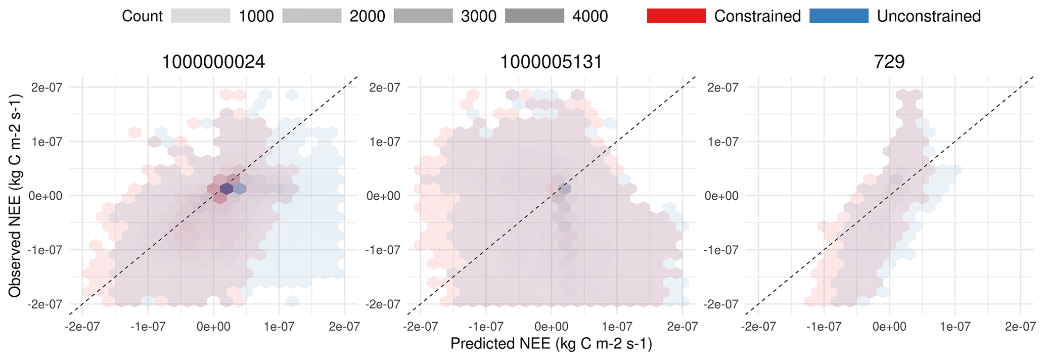
Figure 6A 1:1 plot comparison between observed NEE and simulated NEE for coniferous across all sites and years.
Unconstrained simulations resulted in a large overestimation of NEE in almost all years and for all sites, suggesting either overestimation of total photosynthesis or underestimation of total respiration. Constraining the photosynthesis and respiration parameters (Fig. 5) improved the performance of the model, yet the overall underestimation behavior in the SIPNET model (Table 1) even after calibration points to the inadequacies in the model structure to account for complex interactions among processes.
RMSE estimated in this study for conifer ranged from 39 to KgC m−2 s−1, while the grass PFT ranged 68 to KgC m−2 s−1 across 2006–2011. Fer et al. (2018) estimated a comparable (KgC m−2 s−1) RMSE for the temperate deciduous PFT for 2 years of simulation and across one site. Both model assessment indices suggest that the SIPNET model is more constrained after calibration and ready for use within the state data assimilation routine.
3.2 State data assimilation
As mentioned before, SIPNET represents the terrestrial carbon budget by keeping track of three carbon pools, which are plant wood carbon, plant leaf carbon, and soil carbon, and simulates the major carbon fluxes among these pools (allocation, turnover) as well as between these pools and the atmosphere (photosynthesis, autotrophic, and heterotrophic respiration) (Fig. 1). In our data assimilation procedure, we sequentially assimilated aboveground biomass into the plant wood carbon and leaf area index into the plant leaf carbon on an annual time step, allowing soil carbon to be constrained based on the covariance estimated through the process model. Data assimilation was performed at all the sites at the same time; off-diagonal values in the process model error covariance were adjusted according to Eq. (9).
As an example of the general behavior of the SDA, Fig. 7 shows the reanalysis for a representative conifer site. The initial forecast starting from the BADM initial conditions has a wide posterior distribution and typically a relatively unconstrained mean forecast. The analysis, on the other hand, converges quickly towards the observed AGB and remains thereafter as the compromise between the observation and the model forecast given their uncertainties. If no observation was available, for instance in the case of LAI from the beginning of the simulation until the year 2000 (Fig. 7), the analysis step relied on the covariance estimated among the state variables both within a site and for adjacent sites. The ability to take advantage of the covariances for updating a state variable with no observation allows the SDA to constrain variables, such as soil C, that lack direct, site-level observations at large scales for data assimilation. At the end of each time step, ensemble members were adjusted given the estimated μa and Pa and used as an initial condition for the next time steps.
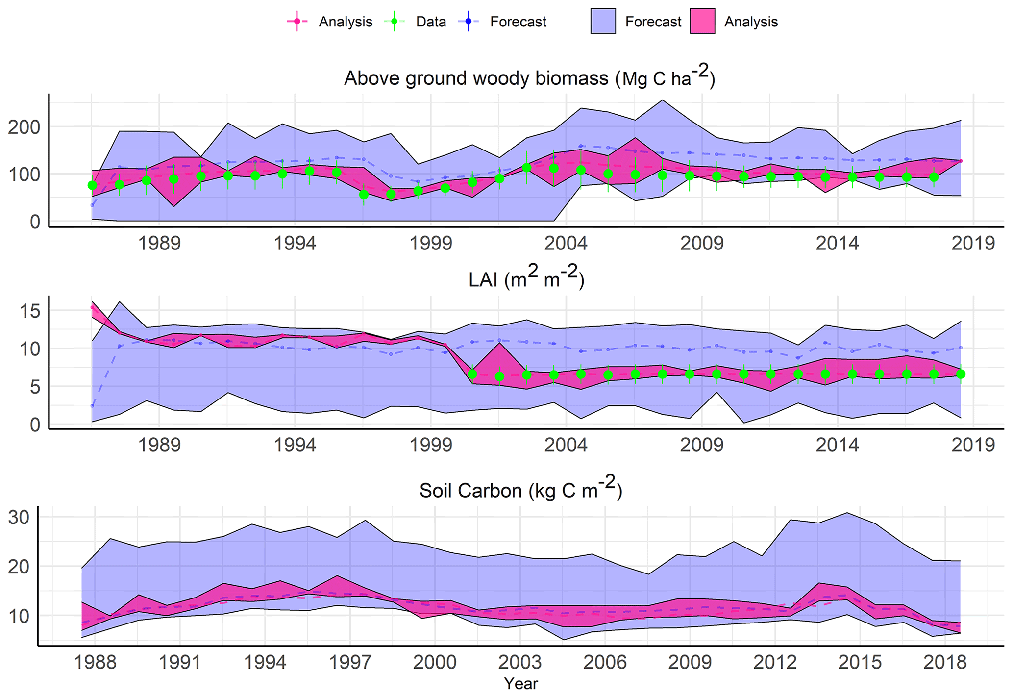
Figure 7Site-level example of sequential data assimilation in an eastern temperate forest ecoregion for a coniferous site (longitude , latitude =33.21).
Starting in the year 2000, we added a second observational constraint, MODIS LAI, after which the analysis LAI contracted considerably around the observations. The soil C pool reanalysis was variable depending on the observation error or uncertainty in the driving forces for different sites and did not show an obvious response to the addition of LAI as a constraint (Fig. 7).
3.2.1 Flux validation and ensemble weighting
The knowledge gained through data assimilation about the state of the carbon pools at each site and year was then transferred post hoc to the flux time series over the preceding time interval by estimating the posterior probability of each ensemble member and using these probabilities to weight each ensemble member. At this stage, no additional observations were used to adjust the model estimates of different carbon fluxes such as NEE (Fig. A2). For example, at the Black Hills AmeriFlux site (Fig. A2), the NEE forecast by SIPNET, which already accounts for the initial condition constraint from the previous SDA step and the parameter constraints from the HPDA, closely followed the observed value. However, adjustment of the model estimates using post hoc weights further improved the predictability of NEE. The effect is not huge, as the current SDA constraint reflects n=2 observations per year; however, the post-adjustment RMSE was reduced by 7.8 % on average for the time period between 2004 and 2009. Adjusting NEE estimates solely based on the weights estimated through data assimilation helped to further close the gap between our forecast and observed NEE even after parameter calibration. The improvements provided by assimilating just two observations per year points to the obvious future directions of increasing both the number of different data constraints and the frequency at which data are assimilated.
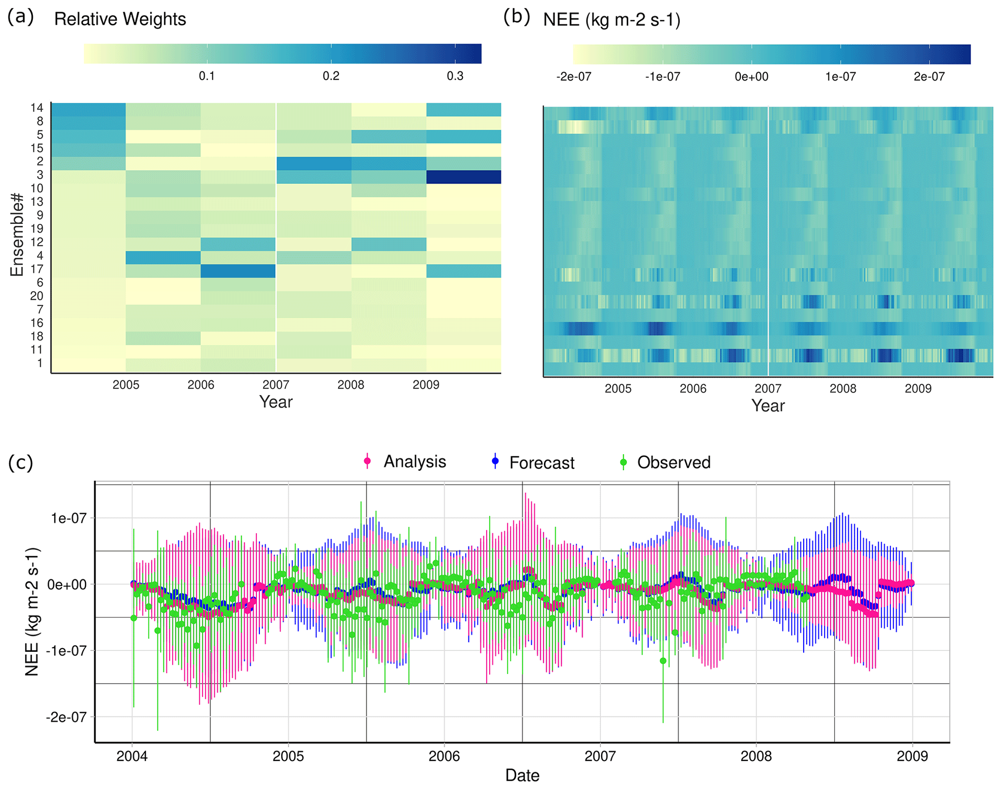
Figure 8(a) Weekly NEE predictions for all ensemble members at the Black Hills site. (b) Relative weight estimated for each ensemble member using Eq. (10) sorted by cumulative weight from highest (top) to lowest (bottom). (c) Weekly average adjusted NEE (analysis) compared to the observed measurements.
Examining the weights assigned to each ensemble member and the flux forecasts associated with them (Fig. A2, top panels) shows two useful patterns. First, there are ensemble members that get consistently low weight, and this includes most of the ensemble members that predict unusual flux time series (e.g., ensemble members 20, 16, and 11). These ensemble members are likely associated with parameter combinations that are not representative of this site (and potentially across sites) and point to a future opportunity to combine simultaneous state estimation and hierarchical parameter constraints (Dokoohaki et al., 2021). This could be done by including the parameters in the analysis and ensemble adjustment, effectively nudging parameters toward more supported values, or through a parameter filtering and resampling, as is done in a particle filter (Dietze, 2017). The second pattern that is apparent in the ensemble weights is that the same ensemble members do not perform the same every year. For example, an ensemble member may perform well one year, only to get very low weight the very next year, but then perform well again a few years later (i.e., ensemble members 2 and 5). To the extent that this reflects variations in parameters, not just initial condition and driver variability, this also suggests that the “best” parameters may vary through time. An important future direction to follow from this is to perform a more in-depth analysis of how model parameter weights vary in both space and time to better understand what parameters are most variable, as this points to processes that are unaccounted for in the underlying models (e.g., if SOM respiration rate varies spatiotemporally it suggests the need to add additional terms to account for this variability). Furthermore, examining the patterns in this variability in space and time can provide important clues about the underlying factors driving variability. Finally, we would need to extend our hierarchical parameter constraint to account for spatiotemporal variability in parameters, as opposed to the current approach that only captures spatial variability.
It is important to note that the patterns of ensemble weights in Fig. A2 reflect the information contribution from the MODIS LAI and LandTrendr AGB constraints, not the information available from the NEE observations themselves. For future applications of this approach, there are other options available to assimilate observed carbon, water, and energy fluxes. The simplest would be to assimilate the cumulative fluxes that have occurred over the time since the previous analysis. We have implemented this approach as part of our site-scale near-term flux forecast, and it introduces the challenge of having to gap-fill the observed fluxes to be able to integrate them. Gap filling introduces uncertainties and causes the assimilation to be, in part, a model–model comparison (process model vs. gap-filling algorithm) instead of a model–data comparison. Assimilating cumulative flux also results in a loss of temporal information and statistical power. Alternatively, we could calculate the likelihood of the observed fluxes for each ensemble member and include this as a weight when calculating the forecast mean and covariance (i.e., μf and Pf). This approach is similar to a particle filter and to ensemble variational data assimilation (Pinnington et al., 2020). For either approach, there are important questions to be explored about the spatial range at which point-level flux observations provide a meaningful constraint on flux reanalysis across landscapes and regions.
3.2.2 Soil C assessment
The degree to which our data assimilation algorithm is able to constrain the soil C pool, which is not observed directly but inferred from the other observations, is related to the quality of AGB and LAI observations at each site, the strength of the covariances between the plant and soil pools, and the overall accuracy of the model. A comparison between the distribution of soil C estimated in this study against the SoilGrids database shows slightly higher mean soil C estimates in this study (13.11 KgC m2 vs. 8.77) but comparable variability across all plant functional types (Fig. 9). The median uncertainty in soil C reanalysis over all sites is between 15 and 20 KgC m−2, and this uncertainty did not change by adding LAI as a new data constraint. Our reanalysis did reasonably well at predicting SOC for the conifer PFT but was consistently higher than corresponding SoilGrids estimates across all other PFTs. Arid grassland showed the largest overestimation with 153 % bias compared to the SoilGrids dataset, whereas the deciduous PFT showed the lowest deviation with only 14 % bias. Furthermore, the largest agreement (index of agreement ∼0.7; Willmott, 1981) was also found in conifer and deciduous PFTs between the two datasets, and the lowest agreement was found to be 0.28 for arid grassland.
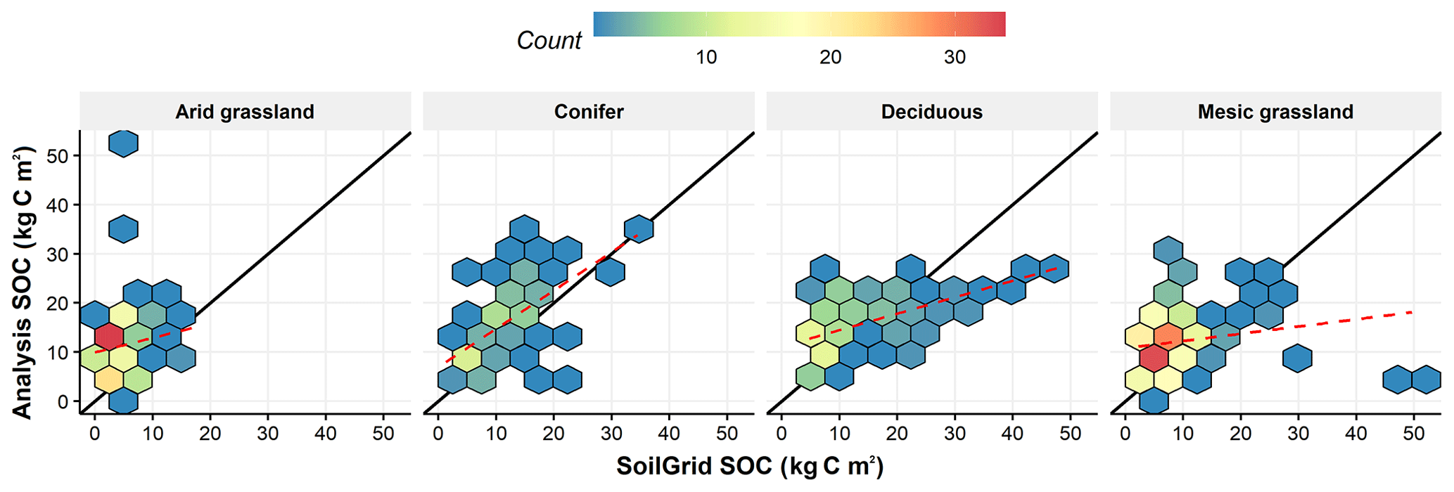
Figure 9Soil organic carbon analysis comparison to the SoilGrids database for different plant functional types. The solid back line represents the one-to-one line, and the dashed red line is the linear regression line between reanalysis SOC in this study and SoilGrids SOC.
On rare occasions (i.e., two sites in arid and three sites in mesic grassland) in this study, we produced estimates of soil C which are not compatible with estimates from other data products such as SoilGrids. This divergence might be attributed to instability in our statistical model at sites with sparse observations. Alternatively, the mismatch between how the soil C pool is defined (i.e., labile versus recalcitrant) between different machine learning and process-based models may complicate the comparison between these data products. It is important to note that this assessment of the performance of our reanalysis does not constitute a true validation because the SoilGrids product is itself a model. But, given that these two studies showed comparable means of the soil C pool across ∼ 500 sites through two different methods with different philosophies, our soil carbon data products can be regarded as a new instrument that allows us to enhance the observational information and to derive higher-level products. In the future, as the spatial resolution of our reanalysis increases, it will be important to perform a more detailed assessment against a wider array of detailed site-level soil data, such as the International Soil Carbon Network's database (Lawrence et al., 2020), the global soil respiration database (Blackard et al., 2008), and the National Ecological Observatory Network.
3.2.3 Forecast uncertainty
One of the notable patterns in our proof-of-concept reanalysis was the tendency for the forecast uncertainty, Pf, to be fairly large despite finding that our reanalysis posteriors had fairly high precision. In part, this occurs because this system is propagating a much broader set of uncertainties than previous studies. Variability in model forecasts can be attributed to the uncertainties in meteorological drivers, model parameters, initial conditions (i.e., analysis posteriors), and the unexplained process error (Dietze, 2017).
We did not find substantial shrinkage in average forecast variability for soil carbon and LAI pools after including the LAI observations in our data assimilation routine (Fig. 10). In other words, adding a second data constraint did not result in a proportional reduction in forecast uncertainty for LAI and soil carbon. However, we noticed a slight reduction in forecast uncertainty for aboveground woody biomass after addition of the second data constraint. Large observation error in MODIS LAI and the inconsistency in scale between the LANDSAT and MODIS resolution could be a few reasons for this observation. Similar findings were reported by Schürmann et al. (2016), wherein multi-stream carbon DA exercises found that a single data stream fit almost as well as multi-data stream assimilation, and by Castro-Morales et al. (2019), wherein the authors found that the largest portion of information came from the first decade of data assimilation, similar to what was found in this study. Altogether, this suggests that initial condition uncertainty is not the dominant driver of forecast uncertainty in the one-step-ahead predictions that occur within the forecast–analysis cycle. Previous site-scale assimilation within the same framework, but with a different model (LINKAGES), found process error, Q, to be a dominant source of forecast uncertainty (Raiho et al., 2020).
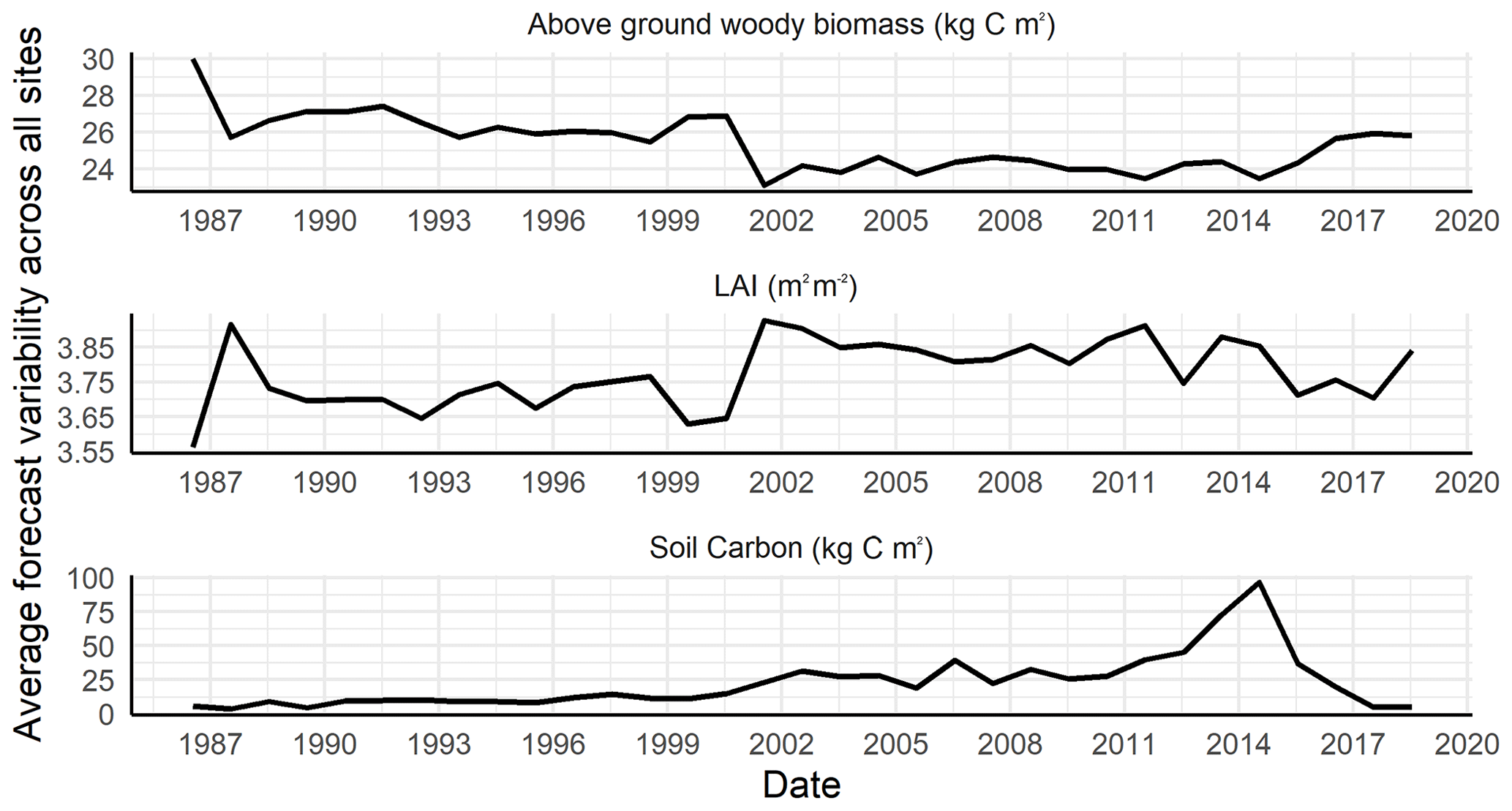
Figure 10Average forecast variability (SD) across all sites and all pools at each time step.
Overall, an important future direction for this work is to perform a detailed uncertainty analysis of the regional-scale reanalysis. Similar to Raiho et al. (2020), this should partition the uncertainties among the four major drivers (initial conditions, drivers, parameters, process error). The dominant uncertainties should then be further partitioned to better understand the contributions of individual processes and parameters (Dietze, 2017, 2014). This feedback will be important for further refining the system, for example prioritizing work among further calibration, additional SDA data constraints, refinement of the mechanistic model, and refinement of the process error covariance model. It may also identify the contributions of uncertainties that are less reducible, such as errors in drivers and stochastic disturbances.
3.2.4 Future directions
While SDA is a valuable tool for producing reanalysis products and improving forecasts, it cannot improve how well the process model represents the system and how often we assimilate new observations. While a simple model like SIPNET presents an opportunity for testing new statistical models for data assimilation and expanding to larger scales, it lacks mechanistic detail around features such as disturbance, phenology, plant carbon partitioning, vegetation composition, structure, and demography, soil and plant hydraulics, and soil carbon dynamics. As a future direction, we will be working towards employing a more advanced vegetation demographic model (Fisher et al., 2018), such as ED2 (Medvigy et al., 2009; Moorcroft et al., 2001), in our data assimilation scheme.
In addition to increasing model sophistication, there are clear arguments for increasing spatial resolution, temporal resolution, the number of ensemble members, and the number of data constraints. However, increasing all of these simultaneously will greatly increase computational demands, especially if we also employ more advanced (and slower) models. Prioritizing which dimensions to focus on first will depend on a number of factors including formal assessments of the computational costs associated with each dimension and the accompanying reductions in uncertainties that each affords.
In terms of increasing the number of data constraints, there are a large number of opportunities available to those interested in carbon cycle reanalysis and forecasting (Baatz et al., 2018). As mentioned earlier, tower fluxes provide a way of anchoring reanalysis estimates of fluxes across broader scales. In addition, there is a clear need to constrain soil C pools and fluxes using a combination of detailed site-scale data and more broad spatial data products. One challenge with assimilating soil C is that most spatial products do not have specific dates associated with them, but rather aggregate data across a broad time range. To assimilate products like this, we will leverage an approach we developed for assimilating fossil pollen data over long timescales (Raiho, 2019) that spreads information over time by inflating the uncertainty such that the effective sample size (and thus information content) is preserved. For CONUS specifically, the USFS Forest Inventory and Analysis also provides additional constraints on biomass and soil C (Blackard et al., 2008).
Beyond field-based measurements, there is also a wealth of remotely sensed data that provide additional constraints. For example, there are a wide range of optical multispectral platforms that could constrain LAI, vegetation type (PFT), and land use change both deeper in the past (e.g., AVHRR, Landsat) and moving forward (e.g., VIIRS, Sentinel-2). Active sensors like lidar (i.e., GEDI, ICESat) and radar (i.e., PalSAR, BIOMASS, NISAR) also provide additional constraints on vegetation height and aboveground biomass. In terms of fluxes, solar-induced fluorescence (i.e., OCO-2, OCO-3, GOME-2, TROPOMI) provides a constraint on GPP, while the same sensors provide column-averaged CO2 estimates that potentially provide a flux constraint on NEE. CO2 concentrations are usually related to land fluxes via complex atmospheric inversions (Ciais et al., 2010), and here, terrestrial carbon reanalyses provide an opportunity to formally reconcile top-down inversion and bottom-up inventory estimates of carbon fluxes and sink attribution.
In addition to direct carbon constraints, there are also a number of remote data products that provide indirect constraints on carbon pools and fluxes. In particular, carbon and water are tightly coupled in many ecosystems (Schlesinger et al., 2016), such as the trade-offs between photosynthetic C update and water loss through transpiration that is measurable via eddy covariance latent heat flux. Microwave remote sensing (e.g., SMAP, SMOS, Sentinel-1C) provides estimates of both soil moisture and vegetation optical depth, the latter providing information on both vegetation biomass and moisture status (Konings et al., 2017, 2019). Finally, imaging spectroscopy (e.g., AVIRIS, DESIS, SBG) provides detailed information about composition, stress, and canopy properties, including the ability to constrain many of the parameters critical to terrestrial ecosystem models (e.g., SLA, Vcmax, leaf N) (Roberts et al., 1997; Shiklomanov et al., 2021).
The localization scheme employed in this study was adopted from climate forecasting research (Reich and Cotter, 2015), wherein the system the authors try to simulate is similar in neighboring cells or simulation blocks. However, a measure of physical distance alone may not be adequate for data assimilation in ecological systems, as two adjacent modeling blocks could represent completely different ecological systems such as different plant functional types or forest stand types. We found that this may substantially affect the process error in the absence of direct observations. This reveals a need and also an opportunity for further exploration of different and more efficient localization schemes in ecological forecasting. Understanding the ability to scale information across space is particularly important for extending this proof of concept to other regions of the world that are less data-dense.
In this study, we presented a proof of concept for a new, synthetic “reanalysis” data product that harmonizes the different components of carbon cycle across the contiguous United States. Overall, our system, which is open-source and extensible to other models, successfully scaled up the new TWEnF assimilation algorithm and PEcAn workflows to provide an unprecedented level of error accounting, including the first estimates of model process error covariance at a national scale. To do so, we developed an efficient approach for assimilating data on an irregular grid and an ensemble weighting approach for updating high-temporal-resolution fluxes. Before running the assimilation, we successfully constrained SIPNET model parameters in a hierarchical Bayesian parameter data assimilation framework using NEE observations from six sites for two PFTs. Next, MODIS LAI and LandTrendr aboveground biomass were sequentially assimilated into the SIPNET model across a network of 493 sites to constrain estimates of carbon pools (leaf, wood, and soil C) and fluxes (GPP, Ra, Rh, NEE). The comparison between our SOC estimates and the SoilGrids data product showed that we have been able to successfully constrain the SOC pools, while comparisons to eddy covariance demonstrated that we were able to constrain net ecosystem exchange. Ultimately, carbon cycle reanalysis should be scalable to a global extent, providing a uniform synthetic platform for carbon monitoring, reporting, and verification (MRV) as well as accelerating terrestrial carbon cycle research.
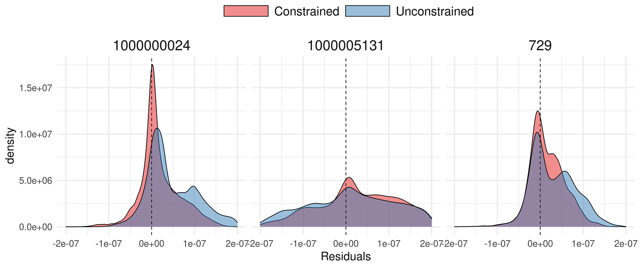
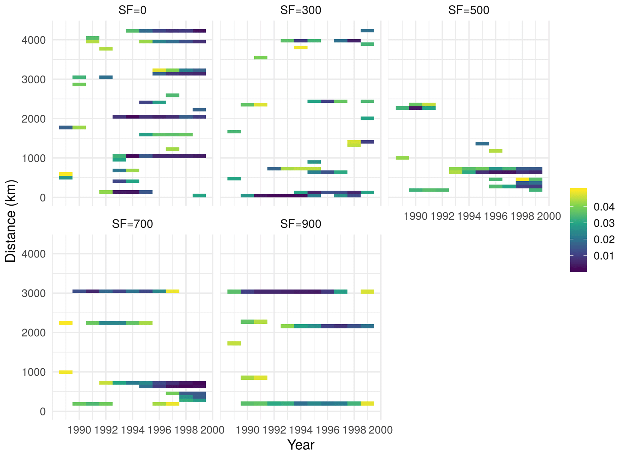
Localization has been found to be one of the most important determining factors in the success of high-dimensional data assimilation problems, especially EnKF (Farchi and Bocquet, 2019). Localization is often applied to either the observation or forecast error covariance matrix with the goal of reducing or removing the spurious correlations that might be generated due to low sample and/or ensemble size. In this study, we used a local support localization method (Eq. 9) adopted from Kalnay and Li (2010), wherein the localization function returns nonzero values for small distances (local region) and zero elsewhere. In order to explore the effect of the scaling factor in Eq. (9), we set up an experimental data assimilation simulation with all 49 AmeriFlux sites and a series of scaling factors (ranging from 0 to 900 km) for the time period between 1989 and 2000. In this experiment, we were interested in finding a scaling factor such that it would produce the lowest spatial autocorrelation in the residuals after the data assimilation. Given our simulation setup, we found that increasing the scaling factor from 0 to 900 km would initially decrease the spatial autocorrelations (Fig. B1) from ν=0 to ν=500 km, and then the autocorrelation would plateau and slightly increase form ν greater than 500 km. Using the ν=500 km with lowest spatial autocorrelation on one hand ensures that our data assimilation algorithm takes advantage of local correlation among similar sites, while, on the other hand it ignores or removes the spurious correlation estimated at larger distances.
The full PEcAn code can be found at https://doi.org/10.5281/zenodo.5557914 (LeBauer et al., 2021).
In addition, pull request numbers 2045, 2481, 2293, 2233, and 2066 on the pecan GitHub repository (https://github.com/pecanproject/pecan/) contain the largest contribution of this work to the PEcAn project. Leaf C, wood C, soil C, NEE, GPP, and autotrophic and heterotrophic respiration data products can also be found using the following link: https://osf.io/efcv5/?view_only=f2eeea87a6504abbae81164efd2b481c (Serbin et al., 2020).
HD was responsible for developing and running the regional-scale data assimilation codes and conducting the study. BDM was responsible for preparing the observed data used in the SDA and the site selection procedure. AR was responsible for developing the site-scale data assimilation code. SPS, and MD were responsible for developing the initial idea and supervising the study. KZ and LD contributed to developing and maintaining site-scale data assimilation code. HD and MD were responsible for writing the paper, and all other authors contributed to revising the paper.
The contact author has declared that neither they nor their co-authors have any competing interests.
Publisher's note: Copernicus Publications remains neutral with regard to jurisdictional claims in published maps and institutional affiliations.
We would also like to acknowledge the work of the PEcAn developer community, specifically Anthony K. Gardella, Elizabeth M. Cowdery, Istem Fer, Alexey N. Shiklomanov, Rob Kooper, and David S. LeBauer, whose contributions to the PEcAn project made this work possible.
This research was supported by NASA CMS under award number 80NSSC17K0711. The PEcAn project is supported by the NSF (ABI no. 1062547, ABI no. 1458021, DIBBS no. 1261582), NASA Terrestrial Ecosystems, the Energy Biosciences Institute, and an Amazon AWS education grant. BDM and SPS were also partially supported by the United States Department of Energy under contract no. DE-SC0012704 to Brookhaven National Laboratory.
This paper was edited by Julia Hargreaves and reviewed by two anonymous referees.
Albergel, C., Calvet, J.-C., Mahfouf, J.-F., Rüdiger, C., Barbu, A. L., Lafont, S., Roujean, J.-L., Walker, J. P., Crapeau, M., and Wigneron, J.-P.: Monitoring of water and carbon fluxes using a land data assimilation system: a case study for southwestern France, Hydrol. Earth Syst. Sci., 14, 1109–1124, https://doi.org/10.5194/hess-14-1109-2010, 2010. a, b
Anderson, J., Hoar, T., Raeder, K., Liu, H., Collins, N., Torn, R., and Avellano, A.: The data assimilation research testbed: A community facility, Bull. Am. Meteorol. Soc., 90, 1283–1296, 2009. a, b
Arakida, H., Miyoshi, T., Ise, T., Shima, S., and Kotsuki, S.: Non-Gaussian data assimilation of satellite-based leaf area index observations with an individual-based dynamic global vegetation model, Nonlin. Processes Geophys., 24, 553–567, https://doi.org/10.5194/npg-24-553-2017, 2017. a, b
Baatz, R., Sullivan, P. L., Li, L., Weintraub, S. R., Loescher, H. W., Mirtl, M., Groffman, P. M., Wall, D. H., Young, M., White, T., Wen, H., Zacharias, S., Kühn, I., Tang, J., Gaillardet, J., Braud, I., Flores, A. N., Kumar, P., Lin, H., Ghezzehei, T., Jones, J., Gholz, H. L., Vereecken, H., and Van Looy, K.: Steering operational synergies in terrestrial observation networks: opportunity for advancing Earth system dynamics modelling, Earth Syst. Dynam., 9, 593–609, https://doi.org/10.5194/esd-9-593-2018, 2018. a
Bacour, C., Peylin, P., MacBean, N., Rayner, P. J., Delage, F., Chevallier, F., Weiss, M., Demarty, J., Santaren, D., Baret, F., and Berveiller, D. : Joint assimilation of eddy covariance flux measurements and FAPAR products over temperate forests within a process-oriented biosphere model, J. Geophys. Res.-Biogeosci., 120, 1839–1857, 2015. a
Battle, M., Bender, M., Tans, P. P., White, J., Ellis, J., Conway, T., and Francey, R.: Global carbon sinks and their variability inferred from atmospheric O2 and δ13C, Science, 287, 2467–2470, 2000. a
Blackard, J., Finco, M., Helmer, E., Holden, G., Hoppus, M., Jacobs, D., Lister, A., Moisen, G., Nelson, M., Riemann, R., Ruefenacht, B., Salajanu, D., Weyermann, D. L., Winterberger, K. C., Breis, T. J., Czaplewski, R. L.,, McRoberts, R. E., Patterson, P. L., and Tymcio, R. P.: Mapping US forest biomass using nationwide forest inventory data and moderate resolution information, Remote Sens. Environ., 112, 1658–1677, 2008. a, b
Braswell, B. H., Sacks, W. J., Linder, E., and Schimel, D. S.: Estimating diurnal to annual ecosystem parameters by synthesis of a carbon flux model with eddy covariance net ecosystem exchange observations, Glob. Change Biol., 11, 335–355, 2005. a
Castro-Morales, K., Schürmann, G., Köstler, C., Rödenbeck, C., Heimann, M., and Zaehle, S.: Three decades of simulated global terrestrial carbon fluxes from a data assimilation system confronted with different periods of observations, Biogeosciences, 16, 3009–3032, https://doi.org/10.5194/bg-16-3009-2019, 2019. a
Cavallaro, N., Shrestha, G., Birdsey, R., Mayes, M., Najjar, R., Reed, S., and Zhu, Z.: Second state of the carbon cycle report (SOCCR2), in: A Sustained Assessment Report, edited by: Cavallaro, N., Shrestha, G., Birdsey, R., Mayes, M. A., Najjar, R. G., Reed, S. C., Romero-Lankao, P., and Zhu, Z., U.S. Global Change Research Program, Washington, DC, USA, 1–4, https://doi.org/10.7930/SOCCR2.2018.Highlights 2018. a
Chen, M., Liu, S., Tieszen, L., and Hollinger, D.: An improved state-parameter analysis of ecosystem models using data assimilation, ecological modelling, 219, 317–326, 2008. a
Ciais, P., Rayner, P., Chevallier, F., Bousquet, P., Logan, M., Peylin, P., and Ramonet, M.: Atmospheric inversions for estimating CO2 fluxes: methods and perspectives, Clim. Change, 103, 69–92, 2010. a
Danabasoglu, G., Lamarque, J.-F., Bacmeister, J., Bailey, D., DuVivier, A., Edwards, J., Emmons, L., Fasullo, J., Garcia, R., Gettelman, A., and Hannay, C.: The Community Earth System Model version 2 (CESM2), J. Adv. Model. Earth Sy., 12, e2019MS001916, 2020. a
Demarty, J., Chevallier, F., Friend, A., Viovy, N., Piao, S., and Ciais, P.: Assimilation of global MODIS leaf area index retrievals within a terrestrial biosphere model, Geophys. Res. Lett., 34, L15402, https://doi.org/10.1029/2007GL030014, 2007. a
de Valpine, P., Turek, D., Paciorek, C., Anderson-Bergman, C., Temple Lang, D., and Bodik, R.: Programming with models: writing statistical algorithms for general model structures with NIMBLE, J. Comput. Graph. Stat., 26, 403–413, https://doi.org/10.1080/10618600.2016.1172487, 2017. a
Dietze, M. C.: Gaps in knowledge and data driving uncertainty in models of photosynthesis, Photosynth. Res., 119, 3–14, 2014. a
Dietze, M. C.: Ecological forecasting, Princeton University Press, 288 p., ISBN 9780691160573, 2017. a, b, c, d, e, f, g
Dokoohaki, H., Miguez, F. E., Archontoulis, S., and Laird, D.: Use of inverse modelling and Bayesian optimization for investigating the effect of biochar on soil hydrological properties, Agr. Water Manage., 208, 268–274, 2018. a
Dokoohaki, H., Kivi, M. S., Martinez-Feria, R. A., Miguez, F. E., and Hoogenboom, G.: A comprehensive uncertainty quantification of large-scale process-based crop modeling frameworks, Environ. Res. Lett., 16, 084010, https://doi.org/10.1088/1748-9326/ac0f26, 2021. a
Evensen, G.: The ensemble Kalman filter for combined state and parameter estimation, IEEE Contr. Syst. Mag., 29, 83–104, 2009. a
Farchi, A. and Bocquet, M.: On the efficiency of covariance localisation of the ensemble Kalman filter using augmented ensembles, Front. App. M. Stat., 5, 3, https://doi.org/10.3389/fams.2019.00003, 2019. a
Fer, I., Kelly, R., Moorcroft, P. R., Richardson, A. D., Cowdery, E. M., and Dietze, M. C.: Linking big models to big data: efficient ecosystem model calibration through Bayesian model emulation, Biogeosciences, 15, 5801–5830, https://doi.org/10.5194/bg-15-5801-2018, 2018. a, b, c, d, e, f, g, h, i, j, k, l, m
Fer, I., Gardella, A. K., Shiklomanov, A. N., Campbell, E. E., Cowdery, E. M., De Kauwe, M. G., Desai, A., Duveneck, M. J., Fisher, J.B., Haynes, K. D., and Hoffman, F. M.: Beyond modeling: A roadmap to community cyberinfrastructure for ecological data-model integration, Glob. Change Biol., 27, 13–26, 2020. a, b
Fer, I., Shiklomanov, A. N., Novick, K. A., Gough, C. M., Arain, M. A., Chen, J., Murphy, B., Desai, A. R., and Dietze, M. C.: Capturing site-to-site variability through Hierarchical Bayesian calibration of a process-based dynamic vegetation model, Cold Spring Harbor Laboratory, bioRxiv, 2021.04.28.441243, https://doi.org/10.1101/2021.04.28.441243, 2021. a
Fisher, R. A., Koven, C. D., Anderegg, W. R., Christoffersen, B. O., Dietze, M. C., Farrior, C. E., Holm, J. A., Hurtt, G. C., Knox, R. G., Lawrence, P. J., Lichstein, J. W., Longo, M., Matheny, A. M., Medvigy, D., Muller-Landau, H. C., Powell, T. L., Serbin, S. P., Sato, H., Shuman, J. K., Smith, B., Trugman, A. T., Viskari, T., Verbeeck, H., Weng, E., Xu, C., Xu, X., Zhang, T., and Moorcroft, P. R.: Vegetation demographics in Earth System Models: A review of progress and priorities, Glob. Change Biol., 24, 35–54, 2018. a
Fox, A. M., Hoar, T. J., Anderson, J. L., Arellano, A. F., Smith, W. K., Litvak, M. E., MacBean, N., Schimel, D. S., and Moore, D. J.: Evaluation of a data assimilation system for land surface models using CLM4. 5, J. Adv. Model. Earth Sy., 10, 2471–2494, 2018. a, b
Gao, C., Wang, H., Weng, E., Lakshmivarahan, S., Zhang, Y., and Luo, Y.: Assimilation of multiple data sets with the ensemble Kalman filter to improve forecasts of forest carbon dynamics, Ecol. Appl., 21, 1461–1473, 2011. a
Hengl, T., Mendes de Jesus, J., Heuvelink, G. B., Ruiperez Gonzalez, M., Kilibarda, M., Blagotić, A., Shangguan, W., Wright, M. N., Geng, X., Bauer-Marschallinger, B., Guevara, M. A., Vargas, R., MacMillan, R. A., Batjes, N. H., Leenaars, J. G. B., Ribeiro, E., Wheeler, I., Mantel, S., and Kempen, B.: SoilGrids250m: Global gridded soil information based on machine learning, PLoS One, 12, e0169748, https://doi.org/10.1371/journal.pone.0169748, 2017. a
Homer, C. H., Fry, J. A., and Barnes, C. A.: The national land cover database, US Geological Survey Fact Sheet, 3020, 1–4, 2012. a
Kalnay, E. and Li, H.: Data Assimilation with the Local Ensemble Transform Kalman Filter addressing model errors, observation errors and adaptive inflation, Saarbrücken: VDM Verlag Dr. Müller, ISBN 9783639308129, https://nbn-resolving.org/urn:nbn:de:101:1-20101108432 (last access: 14 April 2022), 2010. a
Kennedy, R. E., Yang, Z., and Cohen, W. B.: Detecting trends in forest disturbance and recovery using yearly Landsat time series: 1. LandTrendr—Temporal segmentation algorithms, Remote Sens. Environ., 114, 2897–2910, 2010. a
Kennedy, R. E., Yang, Z., Gorelick, N., Braaten, J., Cavalcante, L., Cohen, W. B., and Healey, S.: Implementation of the LandTrendr algorithm on google earth engine, Remote Sens., 10, 691, https://doi.org/10.3390/rs10050691, 2018. a
Kivi, M. S., Blakely, B., Masters, M., Bernacchi, C. J., Miguez, F. E., and Dokoohaki, H.: Development of a data-assimilation system to forecast agricultural systems: A case study of constraining soil water and soil nitrogen dynamics in the APSIM model, Sci. Total Environ., 820, 153192, https://doi.org/10.1016/j.scitotenv.2022.153192, 2022. a
Konings, A. G., Piles, M., Das, N., and Entekhabi, D.: L-band vegetation optical depth and effective scattering albedo estimation from SMAP, Remote Sens. Environ., 198, 460–470, 2017. a
Konings, A. G., Rao, K., and Steele-Dunne, S. C.: Macro to micro: microwave remote sensing of plant water content for physiology and ecology, New Phytol., 223, 1166–1172, 2019. a
Kumar, S. V., M. Mocko, D., Wang, S., Peters-Lidard, C. D., and Borak, J.: Assimilation of remotely sensed leaf area index into the Noah-MP land surface model: Impacts on water and carbon fluxes and states over the continental United States, J. Hydrometeorol., 20, 1359–1377, 2019. a, b
Lawrence, C. R., Beem-Miller, J., Hoyt, A. M., Monroe, G., Sierra, C. A., Stoner, S., Heckman, K., Blankinship, J. C., Crow, S. E., McNicol, G., Trumbore, S., Levine, P. A., Vindušková, O., Todd-Brown, K., Rasmussen, C., Hicks Pries, C. E., Schädel, C., McFarlane, K., Doetterl, S., Hatté, C., He, Y., Treat, C., Harden, J. W., Torn, M. S., Estop-Aragonés, C., Asefaw Berhe, A., Keiluweit, M., Della Rosa Kuhnen, Á., Marin-Spiotta, E., Plante, A. F., Thompson, A., Shi, Z., Schimel, J. P., Vaughn, L. J. S., von Fromm, S. F., and Wagai, R.: An open-source database for the synthesis of soil radiocarbon data: International Soil Radiocarbon Database (ISRaD) version 1.0, Earth Syst. Sci. Data, 12, 61–76, https://doi.org/10.5194/essd-12-61-2020, 2020. a
LeBauer, D., Wang, D., Richter, K. T., Davidson, C. C., and Dietze, M. C.: Facilitating feedbacks between field measurements and ecosystem models, Ecol. Monogr., 83, 133–154, 2013. a, b, c
LeBauer, D., Kooper, R., Mulrooney, P., Rohde, S., Wang, D., Long, S. P., and Dietze, M. C.: BETYdb: A yield, trait, and ecosystem service database applied to second-generation bioenergy feedstock production, GCB Bioenergy, 10, 61–71, 2018. a
LeBauer, D., Dietze, M., Kooper, R., Shiklomanov, A., Cowdery, B., Fer, I., Gardella, A., Bond-Lamberty, B., Serbin, S. P., Raiho, A., Thomas, A., Black, C., Simkins, J., Desai, A., Mantooth, J., Kumar, A., Burke, L., Pourmokhtarian, A., Rollinson, C., Agarwal, S., Hardiman, B., De Kauwe, M., Tess McCabe, E., Ragosta, K., Cohen, T., zhangwenx, Viskari, T., Zhao, Y., and Xia, J: The Predictive Ecosystem Analyzer (PEcAn) is an integrated ecological bioinformatics toolbox, (v1.7.2), Zenodo [code], https://doi.org/10.5281/zenodo.5557914, 2021. a
Ling, X., Fu, C., Guo, W., and Yang, Z.-L.: Assimilation of remotely sensed LAI into CLM4CN using DART, J. Adv. Model. Earth Sy., 11, 2768–2786, 2019. a, b
Liu, S., Bond-Lamberty, B., Hicke, J. A., Vargas, R., Zhao, S., Chen, J., Edburg, S. L., Hu, Y., Liu, J., McGuire, A. D., Xiao, J., Keane, R., Yuan, W., Tang, J., Luo, Y., Potter, C., and Oeding, J.: Simulating the impacts of disturbances on forest carbon cycling in North America: Processes, data, models, and challenges, J. Geophys. Res.-Biogeosci., 116, G00K08, https://doi.org/10.1029/2010JG001585, 2011. a
Liu, Y., Xiao, J., Ju, W., Zhu, G., Wu, X., Fan, W., Li, D., and Zhou, Y.: Satellite-derived LAI products exhibit large discrepancies and can lead to substantial uncertainty in simulated carbon and water fluxes, Remote Sens. Environ., 206, 174–188, 2018. a
Medvigy, D., Wofsy, S., Munger, J., Hollinger, D., and Moorcroft, P.: Mechanistic scaling of ecosystem function and dynamics in space and time: Ecosystem Demography model version 2, J. Geophys. Res.-Biogeosci., 114, G01002, https://doi.org/10.1029/2008JG000812, 2009. a
Mikhailova, E., Altememe, A., Bawazir, A., Chandler, R., Cope, M., Post, C., Stiglitz, R., Zurqani, H., and Schlautman, M.: Comparing soil carbon estimates in glaciated soils at a farm scale using geospatial analysis of field and SSURGO data, Geoderma, 281, 119–126, 2016. a
Montzka, C., Pauwels, V., Franssen, H.-J. H., Han, X., and Vereecken, H.: Multivariate and multiscale data assimilation in terrestrial systems: A review, Sensors, 12, 16291–16333, 2012. a
Moorcroft, P. R., Hurtt, G. C., and Pacala, S. W.: A method for scaling vegetation dynamics: the ecosystem demography model (ED), Ecol. Monogr., 71, 557–586, 2001. a
Morrison, B. D., Heath, K., and Greenberg, J. A.: Spatial scale affects novel and disappeared climate change projections in Alaska, Ecol. Evol., 9, 12026–12044, 2019. a, b
Myneni, R. and Park, Y.: MODIS collection 6 (C6) LAI/FPAR product user’s guide, https://lpdaac.usgs.gov/documents/2/mod15_user_guide.pdf (last access: 5 April 2022), 2015. a, b
Myneni, R. B., Dong, J., Tucker, C. J., Kaufmann, R. K., Kauppi, P. E., Liski, J., Zhou, L., Alexeyev, V., and Hughes, M.: A large carbon sink in the woody biomass of Northern forests, Proc. Natl. Acad. Sci., 98, 14784–14789, 2001. a
Omernik, J. M.: Ecoregions of the conterminous United States, Ann. Assoc. Am. Geogr., 77, 118–125, 1987. a
ORNL DAAC: MODIS and VIIRS Land Products Global Subsetting and Visualization Tool, ORNL DAAC, Oak Ridge, Tennessee, USA, https://doi.org/10.3334/ORNLDAAC/1379, 2018. a
Pan, Y., Birdsey, R. A., Fang, J., Houghton, R., Kauppi, P. E., Kurz, W. A., Phillips, O. L., Shvidenko, A., Lewis, S. L., Canadell, J. G., Ciais, P., Jackson, R. B., Pacala, S. W., Mcguire, A. D., Piao, S., Rautiainen, A., Sitch, S., and Hayes, D.: A large and persistent carbon sink in the world’s forests, Science, 333, 988–993, 2011. a
Petrie, R. E. and Dance, S. L.: Ensemble-based data assimilation and the localisation problem, Weather, 65, 65–69, 2010. a, b
Peylin, P., Bacour, C., MacBean, N., Leonard, S., Rayner, P., Kuppel, S., Koffi, E., Kane, A., Maignan, F., Chevallier, F., Ciais, P., and Prunet, P.: A new stepwise carbon cycle data assimilation system using multiple data streams to constrain the simulated land surface carbon cycle, Geosci. Model Dev., 9, 3321–3346, https://doi.org/10.5194/gmd-9-3321-2016, 2016. a
Pinnington, E., Quaife, T., Lawless, A., Williams, K., Arkebauer, T., and Scoby, D.: The Land Variational Ensemble Data Assimilation Framework: LAVENDAR v1.0.0, Geosci. Model Dev., 13, 55–69, https://doi.org/10.5194/gmd-13-55-2020, 2020. a
Raczka, B., Hoar, T. J., Duarte, H. F., Fox, A. M., Anderson, J. L., Bowling, D. R., and Lin, J. C.: Improving CLM5. 0 biomass and carbon exchange across the Western United States using a data assimilation system, J. Adv. Model. Earth Sy., 13, e2020MS002421, https://doi.org/10.1029/2020MS002421, 2021. a
Raiho, A.: Seeing the Trees through the Forest: Understanding Community Ecology’s Influence on Long Term Ecosystem Dynamics, Order No. 27700991, University of Notre Dame, https://www.proquest.com/dissertations-theses/seeing-trees-through-forest-understanding/docview/2321832430/se-2?accountid=14553 (last access: 19 April 2022), 2019. a
Raiho, A. M., Dietze, M., Dawson, A., Rollinson, C., Tipton, J., and McLachlan, J.: Determinants of Predictability in Multi-decadal Forest Community and Carbon Dynamics, BioRxiv, 2020.05.05.079871, https://doi.org/10.1101/2020.05.05.079871, 2020. a, b, c, d, e, f, g, h, i, j
R Core Team: R: A Language and Environment for Statistical Computing, R Foundation for Statistical Computing, Vienna, Austria, http://www.R-project.org/ (last access: 14 April 2022), 2013. a
Reich, S. and Cotter, C.: Probabilistic forecasting and Bayesian data assimilation, Cambridge University Press, Cambridge, UK, https://doi.org/10.1017/CBO9781107706804, 2015. a, b
Roberts, D., Green, R., and Adams, J.: Temporal and spatial patterns in vegetation and atmospheric properties from AVIRIS, Remote Sens. Environ., 62, 223–240, 1997. a
Schillaci, C., Acutis, M., Lombardo, L., Lipani, A., Fantappie, M., Märker, M., and Saia, S.: Spatio-temporal topsoil organic carbon mapping of a semi-arid Mediterranean region: The role of land use, soil texture, topographic indices and the influence of remote sensing data to modelling, Sci. Total Environ., 601, 821–832, 2017. a
Schlesinger, W. H., Dietze, M. C., Jackson, R. B., Phillips, R. P., Rhoades, C. C., Rustad, L. E., and Vose, J. M.: Forest biogeochemistry in response to drought, Glob. Change Biol., 22, 2318–2328, 2016. a
Scholze, M., Buchwitz, M., Dorigo, W., Guanter, L., and Quegan, S.: Reviews and syntheses: Systematic Earth observations for use in terrestrial carbon cycle data assimilation systems, Biogeosciences, 14, 3401–3429, https://doi.org/10.5194/bg-14-3401-2017, 2017. a, b, c
Schürmann, G. J., Kaminski, T., Köstler, C., Carvalhais, N., Voßbeck, M., Kattge, J., Giering, R., Rödenbeck, C., Heimann, M., and Zaehle, S.: Constraining a land-surface model with multiple observations by application of the MPI-Carbon Cycle Data Assimilation System V1.0, Geosci. Model Dev., 9, 2999–3026, https://doi.org/10.5194/gmd-9-2999-2016, 2016. a, b
Serbin, S., Dokoohaki, H., Morrison, B., Andrews, A., and Dietze, M.: NASA_CMS_SDA, OSF [data set], https://osf.io/efcv5/?view_only=f2eeea87a6504abbae81164efd2b481c (last access: 14 April 2022), 2020. a
Shiklomanov, A. N., Dietze, M. C., Fer, I., Viskari, T., and Serbin, S. P.: Cutting out the middleman: calibrating and validating a dynamic vegetation model (ED2-PROSPECT5) using remotely sensed surface reflectance, Geosci. Model Dev., 14, 2603–2633, https://doi.org/10.5194/gmd-14-2603-2021, 2021. a
Stephenson, N.: Actual evapotranspiration and deficit: biologically meaningful correlates of vegetation distribution across spatial scales, J. Biogeogr., 25, 855–870, 1998. a
Šúri, M. and Hofierka, J.: A new GIS-based solar radiation model and its application to photovoltaic assessments, T. GIS, 8, 175–190, 2004. a
Viskari, T., Hardiman, B., Desai, A. R., and Dietze, M. C.: Model-data assimilation of multiple phenological observations to constrain and predict leaf area index, Ecol. Appl., 25, 546–558, 2015. a, b
Viskari, T., Laine, M., Kulmala, L., Mäkelä, J., Fer, I., and Liski, J.: Improving Yasso15 soil carbon model estimates with ensemble adjustment Kalman filter state data assimilation, Geosci. Model Dev., 13, 5959–5971, https://doi.org/10.5194/gmd-13-5959-2020, 2020. a, b
Wallach, D., Makowski, D., Jones, J., and Brun, F.: Uncertainty and Sensitivity Analysis, edn. 3, Chap. 6, in: Working with Dynamic Crop Models, 13–14, https://doi.org/10.1016/B978-0-12-811756-9.09994-9, 2019. a
Williams, M., Schwarz, P. A., Law, B. E., Irvine, J., and Kurpius, M. R.: An improved analysis of forest carbon dynamics using data assimilation, Glob. Change Biol., 11, 89–105, 2005. a, b
Willmott, C. J.: On the validation of models, Phys. Geogr., 2, 184–194, 1981. a
Xiao, J., Ollinger, S. V., Frolking, S., Hurtt, G. C., Hollinger, D. Y., Davis, K. J., Pan, Y., Zhang, X., Deng, F., Chen, J., Baldocchi, D. D., Law, B. E., Arain, M. A., Desai, A. R., Richardson, A. D., Sun, G., Amiro, B., Margolis, H., Gu, L., Scott, R. L., Blanken, P. D., and Suyker, A. E.: Data-driven diagnostics of terrestrial carbon dynamics over North America, Agr. Forest Meteorol., 197, 142–157, 2014. a
reanalysisproduct that harmonizes carbon pools (leaf, wood, soil) and fluxes (GPP, Ra, Rh, NEE) across the contiguous United States from 1986–2019. Here, we build on a decade of work on uncertainty propagation to generate the most complete and robust uncertainty accounting available to date.