Surface Urban Energy and Water Balance Scheme (v2020a) in vegetated areas: parameter derivation and performance evaluation using FLUXNET2015 dataset

To compare the impact of surface–atmosphere exchanges from rural and urban areas, fully vegetated areas (e.g. deciduous trees, evergreen trees and grass) commonly found adjacent to cities need to be modelled. Here we provide a general workflow to derive parameters for SUEWS (Surface Urban Energy and Water Balance Scheme), including those associated with vegetation phenology (via leaf area index, LAI), heat storage and surface conductance. As expected, attribution analysis of bias in SUEWS-modelled Q_E finds that surface conductance (g_s) plays the dominant role; hence there is a need for more estimates of surface conductance parameters. The workflow is applied at 38 FLUXNET sites. The derived parameters vary between sites with the same plant functional type (PFT), demonstrating the challenge of using a single set of parameters for a PFT. SUEWS skill at simulating monthly and hourly latent heat flux (Q_E) is examined using the site-specific derived parameters, with the default NOAH surface conductance parameters (Chen et al., 1996). Overall evaluation for 2 years has similar metrics for both configurations: median hit rate between 0.6 and 0.7, median mean absolute error less than 25 W m⁻², and median mean bias error ∼ 5 W m⁻². Performance differences are more evident at monthly and hourly scales, with larger mean bias error (monthly: ∼ 40 W m⁻²; hourly ∼ 30 W m⁻²) results using the NOAH-surface conductance parameters, suggesting that they should be used with caution. Assessment of sites with contrasting Q_E performance demonstrates how critical capturing the LAI dynamics is to the SUEWS prediction skills of g_s and Q_E. Generally g_s is poorest in cooler periods (more pronounced at night, when underestimated by ∼ 3 mm s⁻¹). Given the global LAI data availability and the workflow provided in this study, any site to be simulated should benefit.

1 Introduction

The Surface Urban Energy and Water Balance Scheme (SUEWS, Grimmond et al., 1986, 1991; Grimmond and Oke, 1991; Järvi et al., 2011) is widely used to simulate urban surface energy and hydrological fluxes, with heat and water released by anthropogenic activities accounted for (Grimmond et al., 1986; Grimmond, 1992). SUEWS characterises the heterogeneity of urban surfaces allowing an integrated mix of seven land covers within a grid cell (neighbourhood scale: O(0.1–10 km)) of impervious (buildings, paved) and pervious (evergreen trees/shrubs, deciduous trees/shrubs, grass, soil, water) types. Although SUEWS has been evaluated in cities around the globe (e.g. Karsisto et al., 2016; Ward et al., 2016; Ao et al., 2018; Kokkonen et al., 2018; Harshan et al., 2018) with varying mixes of integrated impervious–pervious land covers, its performance has not been comprehensively examined in fully vegetated areas that commonly occur adjacent to cities.

One common and demanding application of urban climate models, including SUEWS, is to examine the very well-known canopy-layer urban heat island effects – parts of cities are often warmer than their surroundings at night – and to understand the causes (Oke, 1973, 1982). This requires both the “rural” context – usually characterised by pervious land cover – and the urban area of focus to be simulated appropriately ideally using the same modelling framework. As SUEWS v2020a (Tang et al., 2021) can diagnose near-surface meteorology in the roughness sub-layer and canopy layer (e.g. air temperature and humidity at 2 $\mathrm{m}\mathrm{a}.\mathrm{g}.\mathrm{l}.$ (above ground level), wind speed at 10 $\mathrm{m}\mathrm{a}.\mathrm{g}.\mathrm{l}.$), it is essential to ensure that any urban–rural comparison in these diagnostics has the proper rural skill and parameters (i.e. coefficient values used in parameterisations).

For meso-scale numerical weather prediction (NWP) of an urban region, both rural and urban areas need to be simulated. With plans to couple SUEWS to a meso-scale model (e.g. Weather Research and Forecasting (WRF); Skamarock and Klemp, 2008), most regions have extensive areas that have completely pervious grid cells. As these need to be simulated using a consistent surface scheme, it is essential to have appropriate parameters for these areas.

Central to the SUEWS biophysics is the Penman–Monteith approach (Penman, 1948; Monteith, 1965) with a Jarvis-type (Jarvis, 1976) surface moisture conductance (Grimmond and Oke, 1991). Parameters for different types of urban areas (e.g. land cover differences) and regions (e.g. high latitude or mid-latitude) have been derived. However, both limited observations and lack of a standard workflow for deriving parameters remain a constraint. This is evident in the availability of conductance- and storage-heat-flux-related parameters (e.g. Järvi et al., 2011, 2014; Ward et al., 2016). Other land surface schemes have parameters for a wide range of plant functional types (PFTs) (e.g. NOAH within WRF,r Chen et al., 1996; Chen and Dudhia, 2001) but are often derived from a small number of observational sites, and their widespread applicability is unexamined. For example, NOAH largely adopted values from the HAPEX-MOBILHY observational program (Andre et al., 1986) following Noilhan and Planton (1989).

FLUXNET (Baldocchi et al., 2001) is a global network of sites that monitor surface–atmosphere exchanges (e.g. carbon, water, and energy turbulent fluxes using the eddy covariance technique). These data provide unprecedented possibilities to advance process-based land surface modelling, through both development (e.g. Stöckli et al., 2008) and evaluation (e.g. Zhang et al., 2017). Extensive analysis of FLUXNET datasets for the variety of terrestrial PFTs have considered various surface atmosphere controls (e.g. albedo: Cescatti et al., 2012; latent heat flux: Ershadi et al., 2014; spatiotemporal representativeness: Chu et al., 2017; Villarreal and Vargas, 2021; energy balance closure: Franssen et al., 2010; landscape heterogeneity: Göckede et al., 2008; Stoy et al., 2013) to enhance understanding of land–atmosphere interactions. As such, this is an ideal data source for deriving widely applicable parameters and assessing performance of SUEWS over different land cover types.

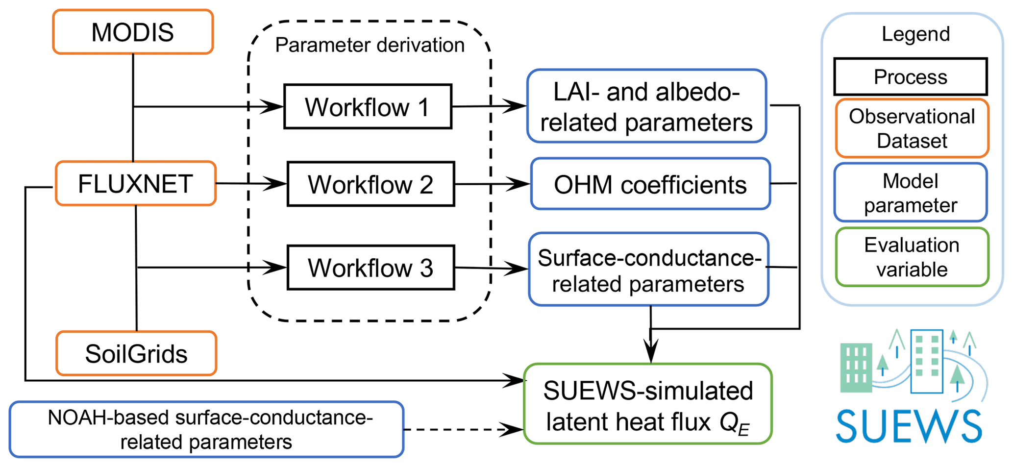
Figure 1 Overview of workflows to derive parameters and to undertake and to evaluate simulations. Acronyms are defined in Sects. 2 and 3. More details are provided in Figs. 3, 5 and 6.

In this work, we develop general workflows (Fig. 1) to derive vegetation-related parameters associated with phenology, the storage heat flux and surface moisture conductance and comprehensively examine model skill in modelling latent heat fluxes. We briefly review the key vegetation biophysics schemes in SUEWS (Sect. 2), describe the FLUXNET2015 (Pastorello et al., 2020) and auxiliary datasets used (Sect. 3), and outline the workflows for deriving parameters (Sect. 4). To assess the quality of the derived parameters the SUEWS-modelled latent heat flux is evaluated (Sect. 5). Model parameters related to surface conductance are derived for NOAH at the PFT level (Appendix A) as well as those related to surface roughness based on the FLUXNET2015 dataset at the site level (Appendix B). Other model parameters derived following workflows (Sect. 4) are also provided (Appendix C). The source code, input data and model simulations analysed are provided in Sun et al. (2021).

2 SUEWS model

2.1 Overview of SUEWS physics for vegetated areas

The Surface Urban Energy and Water Balance Scheme (SUEWS) is a local-scale land surface model for simulating the surface energy and hydrological fluxes (Grimmond and Oke, 1986, 1991; Järvi et al., 2011, 2014; Offerle et al., 2003; Ward et al., 2016) without requiring specialised computing facilities. It has been extensively evaluated and applied in many cities (Lindberg et al., 2018, their Table 3; Sun and Grimmond, 2019, their Table 1). Other details of how SUEWS computes the surface energy, water and carbon fluxes are given in recent model description papers (Järvi et al., 2011, 2019; Ward et al., 2016).

The surface energy and water balances are directly linked by the turbulent latent heat flux (Q_E) or its mass equivalent evaporation (E) (Grimmond and Oke, 1986, 1991):

$$\begin{array}{}\text{(1)}& {\displaystyle }{Q}^{\ast }+Q_{\mathrm{F}}=Q_{\mathrm{H}}+Q_{\mathrm{E}}+\mathrm{\Delta }{Q}_{\mathrm{S}},\text{(2)}& {\displaystyle }P+I_{\mathrm{e}}=E+R+\mathrm{\Delta }S,\end{array}$$

where Q^∗ is the net all-wave radiation flux; Q_F is the anthropogenic heat flux; Q_H is the turbulent sensible heat flux; ΔQ_S the net storage heat flux; and P, I_e, ΔS and R are precipitation, external water use, net change in the water storage (e.g. canopy, soil moisture, water bodies) and runoff, respectively. The sites selected in this work are assumed to have no irrigation, so I_e is assumed to be 0 mm s⁻¹.

In SUEWS, a modified Penman–Monteith equation (Penman, 1948; Monteith, 1965) is used to compute Q_E with an expectation in cities that the anthropogenic heat flux (Q_F) is greater than zero (Grimmond and Oke, 1991):

$$\begin{array}{}\text{(3)}& Q_{\mathrm{E}}={\displaystyle \frac{s\left(Q^{\ast }+Q_{\mathrm{F}}-\mathrm{\Delta }{Q}_{\mathrm{S}}\right)+\frac{\mathit{\rho }{c}_{\mathrm{p}}\text{VPD}}{r_{\mathrm{a}}}}{s+\mathit{\gamma }\left(\mathrm{1}+\frac{r_s}{r_{\mathrm{a}}}\right)}}.\end{array}$$

However, with our current focus on extensive (non-urban) pervious areas Q_F is assumed to be 0 W m⁻². The atmospheric state is obtained from the slope of saturation water vapour pressure curve with respect to air temperature (s, Pa K⁻¹), density of air (ρ, kg m⁻³), specific heat of air at constant pressure (c_p, $\mathrm{J}{\mathrm{K}}^{-\mathrm{1}}{\mathrm{kg}}^{-\mathrm{1}}$), vapour pressure deficit (VPD, Pa), psychrometric “constant” (γ, Pa K⁻¹) and the aerodynamic resistance for water vapour (r_a,  s m⁻¹).

Table 1 Parameters and the first process they are used in by SUEWS (i.e. most impact multiple variables). Sources (S) include this study (^∗), Ward et al. (2016) (W16) and FLUXNET2015 (F15, Pastorello et al., 2020) where values are given or used in individual equations (Eq.). Two key phenology periods are related to growing and senescence degree days (GDD, SDD).

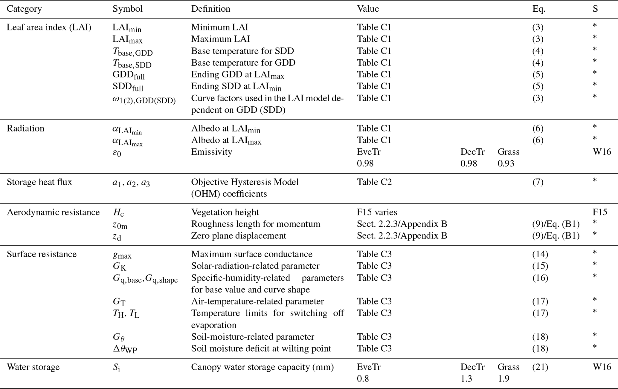
Under given ambient meteorological conditions (e.g. incoming solar radiation K_↓, air temperature T_a, humidity) at an extensive vegetated site, Q_E from this method is sensitive to the estimation of available energy (i.e. $Q^{\ast }-\mathrm{\Delta }{Q}_{\mathrm{S}}$), aerodynamic resistance r_a and surface resistance r_s. Hence, the critical vegetation-related parameters (Table 1) are addressed with these caveats and/or assumptions:

• Surface emissivity ε₀ and canopy water storage capacity S_i are assumed to be the same as reported in Ward et al. (2016).

• Aerodynamic resistance r_a is highly dependent on aerodynamic parameters that vary with canopy height (H_c) and leaf area index (LAI) (Kent et al., 2017a, b; Appendix B). The temporally varying H_c is obtained from FLUXNET2015 (Sect. 2.2.3). LAI varies with phenology (Sect. 2.2.1).

2.2 Q_E-related sub-schemes in SUEWS

2.2.1 Leaf area index (LAI) and radiation

In SUEWS, leaf growth is triggered by reaching a critical growing-degree-day (GDD) threshold $(T_{\text{base},\text{GDD},i}$), and similarly for leaf fall by senescence degree days (SDDs, $T_{\text{base},\text{SDD},i}$) using daily (d) mean air temperatures (T_d) based on the previous day (d−1) for each vegetation type i (one of evergreen trees, deciduous trees and grass). For forests and grass we use the following (Järvi et al., 2011):

$$\begin{array}{}\text{(4)}& \begin{array}{rl}& {\text{LAI}}_{\mathrm{d},i}=\\ & \left\{\begin{array}{l}min({\text{LAI}}_{max,i},{\text{LAI}}_{d-\mathrm{1},i}^{{\mathit{\omega }}_{\mathrm{1},\text{GDD},i}}{\text{GDD}}_{d,i}{\mathit{\omega }}_{\mathrm{2},\text{GDD},i}\\ +{\text{LAI}}_{d-\mathrm{1},i}),T_{\text{base},\text{SDD},i}<T_{d-\mathrm{1}}<T_{\text{base},\text{GDD},i}\\ max({\text{LAI}}_{min,i},{\text{LAI}}_{d-\mathrm{1},i}{\mathit{\omega }}_{\mathrm{1},\text{SDD},i}(\mathrm{1}-{\text{SDD}}_{d,i}){\mathit{\omega }}_{\mathrm{2},\text{SDD},i}\\ +{\text{LAI}}_{d-\mathrm{1},i}),T_{\text{base},\text{GDD},i}<T_{d-\mathrm{1}}<T_{\text{base},\text{SDD},i},\end{array}\right.\end{array}\end{array}$$

with ${\mathit{\omega }}_{\mathrm{1}/\mathrm{2},\text{GDD}/\text{SDD},i}$ curve factors needing to be derived. T_d−1 is derived from the daily maximum ($T_{\mathrm{a}}^{max}$) and minimum ($T_{\mathrm{a}}^{min}$) air temperature of the previous day:

$$\begin{array}{}\text{(5)}& T_{d-\mathrm{1}}={\displaystyle \frac{T_{\mathrm{a}}^{max}+T_{\mathrm{a}}^{min}}{\mathrm{2}}}.\end{array}$$

For each site and vegetation type i, the maximum and minimum LAI values (${\text{LAI}}_{max,i}$, ${\text{LAI}}_{min,i}$) and T_base,GDD and T_base,SDD are determined for each site (Sect. 4.1). For sites at higher latitude (e.g. > 60^∘), other characteristics – such as day length and photo period – are helpful to account for corresponding LAI controls (Bauerle et al., 2012; Gill et al., 2015).

LAI influences several processes in SUEWS – such as dynamics of surface conductance (later in Sect. 2.2.4) and albedo – the latter varies with daily LAI between a minimum (${\mathit{\alpha }}_{{\text{LAI}}_{min}}$) and maximum (${\mathit{\alpha }}_{{\text{LAI}}_{max}}$) by vegetation type:

$$\begin{array}{}\text{(6)}& \begin{array}{rl}{\mathit{\alpha }}_{d,i}& ={\mathit{\alpha }}_{d-\mathrm{1},i}+\left({\mathit{\alpha }}_{\text{LAI},max,i}-{\mathit{\alpha }}_{\text{LAI},min,i}\right)\\ & \times {\displaystyle \frac{{\text{LAI}}_{d,i}-{\mathrm{LAI}}_{d-\mathrm{1},i}}{{\text{LAI}}_{max,i}-{\text{LAI}}_{min,i}}}.\end{array}\end{array}$$

We note the SUEWS urban snow module (Järvi et al., 2014) is not used in this work, so we focus on snow-free conditions. This may bias some modelled α and subsequent fluxes, but evaluating the snow module is a large task in its own right.

Within SUEWS the albedo is used with the observed incoming shortwave radiation and longwave radiation to obtain Q^∗. In the current analyses, the observed incoming longwave (L_↓) and modelled outgoing longwave radiation ($L_{\uparrow }=(\mathrm{1}-{\mathit{\epsilon }}_{\mathrm{0}})L_{\downarrow }+{\mathit{\epsilon }}_{\mathrm{0}}\mathit{\sigma }{T}_{\mathrm{s}}^{\mathrm{4}}$, where ε₀ is the surface emissivity; σ is the Stefan Boltzmann constant, $\mathrm{W}{\mathrm{m}}^{-\mathrm{2}}{\mathrm{K}}^{-\mathrm{4}}$; and T_s is the surface temperature, K) are used. Table 1 gives the emissivity values used.

2.2.2 Storage heat flux

Storage heat flux ΔQ_S is simulated with the objective hysteresis model (OHM, Grimmond et al., 1991):

$$\begin{array}{}\text{(7)}& \mathrm{\Delta }{Q}_{\mathrm{S}}=\sum _i{f}_i\left[a_{\mathrm{1},i}{Q}^{\ast }+a_{\mathrm{2},i}{\displaystyle \frac{\partial Q^{\ast }}{\partial t}}+a_{\mathrm{3},i}\right],\end{array}$$

where f_i is the plan area (or three-dimensional fraction area, Grimmond et al., 1991; Grimmond and Oke, 1999) fraction of surface i, a₁₋₃ are the OHM coefficients (Sect. 4.2), and t is time.

2.2.3 Aerodynamic resistance

Aerodynamic resistance r_a is obtained from Järvi et al. (2011) and van Ulden and Holtslag (1985):

$$\begin{array}{}\text{(8)}& r_{\mathrm{a}}={\displaystyle \frac{\left[\ln \left(\frac{z_{\mathrm{m}}-z_{\mathrm{d}}}{z_{\mathrm{0}\mathrm{m}}}-{\mathit{\psi }}_{\mathrm{m}}\left(\mathit{\zeta }\right)\right)\right]\left[\ln \left(\frac{z_{\mathrm{m}}-z_{\mathrm{d}}}{z_{\mathrm{0}\mathrm{v}}}-{\mathit{\psi }}_{\mathrm{v}}\left(\mathit{\zeta }\right)\right)\right]}{{\mathit{\kappa }}^{\mathrm{2}}u}},\end{array}$$

where z_m is the measurement height for mean wind speed (u) and κ the von Kármán constant (0.4 assumed); the aerodynamic parameters z_d (zero plane displacement height) and z_0m (roughness length for the momentum) are estimated as a function of canopy height H_c (Garratt, 1992; Grimmond and Oke, 1999):

$$\begin{array}{}\text{(9)}& {\displaystyle }{z}_{\mathrm{0}\mathrm{m}}=f_{\mathrm{0}}{H}_{\mathrm{c}},\text{(10)}& {\displaystyle }{z}_{\mathrm{d}}=f_{\mathrm{d}}{H}_{\mathrm{c}},\end{array}$$

with f₀ and f_d being vegetation-based coefficients (see Appendix B for derivation details). The stability parameter ζ ($=(z_{\mathrm{m}}-z_{\mathrm{d}})/L$) depends on the Obukhov length L. The atmospheric stability functions of momentum (ψ_m) and water vapour (ψ_v) for unstable conditions are (Campbell and Norman, 1998)

$$\begin{array}{c}{\displaystyle }{\mathit{\psi }}_{\mathrm{v}}=\mathrm{2}\ln \left[{\displaystyle \frac{\mathrm{1}+(\mathrm{1}-\mathrm{16}\mathit{\zeta }{)}^{\mathrm{1}/\mathrm{2}}}{\mathrm{2}}}\right],\\ \text{(11)}& {\displaystyle }{\mathit{\psi }}_{\mathrm{m}}=\mathrm{0.6}{\mathit{\psi }}_{\mathrm{v}},\end{array}$$

and for stable conditions (Campbell and Norman, 1998; Högström, 1988)

$$\begin{array}{}\text{(12)}& \begin{array}{rl}& {\mathit{\psi }}_{\mathrm{v}}=-\mathrm{4.5}\ln (\mathrm{1}+\mathit{\zeta }),\\ & {\mathit{\psi }}_{\mathrm{m}}=-\mathrm{6}\ln (\mathrm{1}+\mathit{\zeta }).\end{array}\end{array}$$

2.2.4 Surface resistance (r_s) or conductance (g_s)

For completely wet surfaces, the surface resistance r_s is assumed to be 0 s m⁻¹ (i.e. potential evaporation is calculated from Eq. 3). Otherwise r_s, or its inverse, surface conductance g_s, is parameterised with a Jarvis-type formulation (Jarvis, 1976) in SUEWS (Grimmond and Oke, 1991; Järvi et al., 2011; Ward et al., 2016):

$$\begin{array}{}\text{(13)}& \begin{array}{rl}{r}_{\mathrm{s}}^{-\mathrm{1}}& =g_{\mathrm{s}}\\ & ={\sum }_i(g_{\text{max},i}\cdot f_i\cdot g({\text{LAI}}_i\left)\right)g\left(K_{\downarrow }\right)g\left(\mathrm{\Delta }q\right)g\left(T_{\mathrm{a}}\right)g\left(\mathrm{\Delta }{\mathit{\theta }}_{\text{soil}}\right),\end{array}\end{array}$$

where g_s is determined from the ith land cover areally weighted maximum surface conductance ($g_{max,i}$) (with f_i=1 for a “homogeneous” site) and environmental (x) rescaling functions (g(x)) ranging between [0, 1], including the following:

• Leaf area index (LAI) (Ward et al., 2016).

  $$\begin{array}{}\text{(14)}& g\left({\text{LAI}}_i\right)={\displaystyle \frac{{\text{LAI}}_i}{{\text{LAI}}_{max,i}}},\end{array}$$

  which is relative to the maximum LAI of land cover i (${\text{LAI}}_{max,i}$). For bare soil surfaces (i.e. no vegetation), when LAI is irrelevant g(LAI_i)=1.

• Incoming shortwave radiation (K_↓) (Stewart, 1988).

  $$\begin{array}{}\text{(15)}& g\left(K_{\downarrow }\right)={\displaystyle \frac{\frac{K_{\downarrow }}{G_{\mathrm{K}}+K_{\downarrow }}}{\frac{K_{\downarrow ,max}}{G_{\mathrm{K}}+K_{\downarrow ,max}}}},\end{array}$$

  where the G_K parameter modifies the K_↓ response, relative to $K_{\downarrow ,max}$ the maximum observed incoming shortwave radiation (= 1200 W m⁻²): when K_↓ approaches G_K, g(K_↓) reaches 50 % of $g_{s,max}(\frac{K_{\downarrow ,max}}{G_{\mathrm{K}}+K_{\downarrow ,max}}{)}^{-\mathrm{1}}$ (i.e. $g_{s,max}$ normalised by $\frac{K_{\downarrow ,max}}{G_{\mathrm{K}}+K_{\downarrow ,max}}$). At night g(K_↓) goes to 1.

• Specific humidity deficit (Δq​​​​​​​) (Ogink-Hendriks, 1995).

  $$\begin{array}{}\text{(16)}& g\left(\mathrm{\Delta }q\right)=G_{\mathrm{q},\text{base}}+(\mathrm{1}-G_{\mathrm{q},\text{base}})G_{\mathrm{q},\text{shape}}^{\mathrm{\Delta }q},\end{array}$$

  where the specific-humidity-related parameters are for the “base” G_q,base and curve shape G_q,shape: the former indicates the limit of g(Δq) when Δq approaches extremely large values, while the latter determines the curvature of the g(Δq) (e.g. Fig. 9c).

• Air temperature (T_a) (Stewart, 1988).

  $$\begin{array}{}\text{(17)}& g\left(T_{\mathrm{a}}\right)={\displaystyle \frac{(T_{\mathrm{a}}-T_{\mathrm{L}})(T_{\mathrm{H}}-T_{\mathrm{a}}{)}^{T_{\mathrm{c}}}}{(G_{\mathrm{T}}-T_{\mathrm{L}})(T_{\mathrm{H}}-G_{\mathrm{T}}{)}^{T_{\mathrm{c}}}}},\end{array}$$

  where $T_{\mathrm{c}}=\frac{T_{\mathrm{H}}-G_{\mathrm{T}}}{G_{\mathrm{T}}-T_{\mathrm{L}}}$ is a function of the lower (T_L) and upper (T_H) limits when the evaporation occurs, and G_T the optimal temperature for evaporation to reach its potential maximum.

• Soil moisture deficit (Δθ_soil, difference between soil water capacity and soil moisture content) (Ward et al., 2016).

  $$\begin{array}{}\text{(18)}& g\left(\mathrm{\Delta }{\mathit{\theta }}_{\text{soil}}\right)={\displaystyle \frac{\mathrm{1}-\exp \left(G_{\mathit{\theta }}\right(\mathrm{\Delta }{\mathit{\theta }}_{\text{soil}}-\mathrm{\Delta }{\mathit{\theta }}_{\text{WP}}\left)\right)}{\mathrm{1}-\exp (-G_{\mathit{\theta }}\mathrm{\Delta }{\mathit{\theta }}_{\text{WP}})}}.\end{array}$$

  Both the wilting point (Δθ_WP) and a soil-type-dependent parameter (G_θ) vary with soil and plant type.

Appendix A gives the equivalent form used in the NOAH model for Eq. (13).

SUEWS has a running water balance that accounts for the multiple surface types. The amount of water on the canopy of each surface (C_i) (Grimmond and Oke, 1991) is used to vary the surface resistance between dry and wet (r_s = 0 s m⁻¹) by replacing r_s with r_ss (Shuttleworth, 1978):

$$\begin{array}{}\text{(19)}& r_{\text{ss}}={\left[{\displaystyle \frac{W}{r_{\mathrm{b}}(s/\mathit{\gamma }+\mathrm{1})}}+{\displaystyle \frac{(\mathrm{1}-W)}{r_{\mathrm{s}}+r_{\mathrm{b}}(s/\mathit{\gamma }+\mathrm{1})}}\right]}^{-\mathrm{1}}-r_{\mathrm{b}}(s/\mathit{\gamma }+\mathrm{1}),\end{array}$$

where W is a function of the relative amount of water present on each surface to its water storage capacity (S_i, Table 1):

$$\begin{array}{}\text{(20)}& \begin{array}{rlrl}& W=\mathrm{1}& & C_i\ge S_{\mathrm{i}},\\ & W={\displaystyle \frac{K-\mathrm{1}}{K-S_{\mathrm{i}}/C_i}}& & C_i<S_{\mathrm{i}}.\end{array}\end{array}$$

K depends on the aerodynamic and surface resistances:

$$\begin{array}{}\text{(21)}& K={\displaystyle \frac{(r_{\mathrm{s}}/r_{\mathrm{a}})/(r_{\mathrm{a}}-r_{\mathrm{b}})}{r_{\mathrm{s}}+r_{\mathrm{b}}(s/\mathit{\gamma }+\mathrm{1})}},\end{array}$$

where r_b, the boundary layer resistance, is a function of friction velocity u_∗ (Shuttleworth, 1983):

$$\begin{array}{}\text{(22)}& r_{\mathrm{b}}=\mathrm{1.1}{u}_{\ast }^{-\mathrm{1}}+\mathrm{5.6}{u}_{\ast }^{\frac{\mathrm{1}}{\mathrm{3}}}.\end{array}$$

Equations (19)–(22) ensure that the surface resistance r_ss has a smooth transition from 0 (a completely wet surface) to r_s (a dry surface).

3 Global observational datasets used

We use three global datasets FLUXNET2015 (Pastorello et al., 2020), MODIS (Myneni et al., 2015) and SoilGrids (Hengl et al., 2014) to derive the parameters. The FLUXNET2015 surface energy fluxes and other meteorology observations are used for three purposes: to derive parameter values, force simulations and evaluate simulations. The remotely sensed (MODIS) derived LAI products are used for the LAI-related parameters. To derive soil-moisture-related parameters the SoilGrids data are used. Unlike the FLUXNET2015 data, the latter two datasets are spatially continuous.

3.1 FLUXNET2015

The FLUXNET2015 dataset (Pastorello et al., 2020) is the newest version of the FLUXNET data products. The gap-filled dataset includes 212 flux sites from around the world. Although the FLUXNET focus is on local-scale ecosystem CO₂ eddy covariance (EC) fluxes, it also includes water and energy EC fluxes plus other meteorological and biological data. The biosphere–atmosphere exchange dataset contains more than 1500 site years for the period to the end of 2014. The open-source package ONEFlux (Open Network-Enabled Flux processing pipeline; https://github.com/fluxnet/ONEFlux, last access: 4 November 2021) is used to produce FLUXNET2015 (Pastorello et al., 2020).

Table 2 FLUXNET2015 (Pastorello et al., 2020) variables used in this work to derive parameters (P), to force (F) model simulations and to evaluate (E) models.

Table 3 Key information about the FLUXNET2015 sites (Pastorello et al., 2020, and their DOI reference used in this work; site name, country name, with altitude above sea level, $\mathrm{a}.\mathrm{s}.\mathrm{l}.$) or anemometer sensor height above ground level ($\mathrm{a}.\mathrm{g}.\mathrm{l}.$). More details about the simulation and analyses given in Sect. 5.1. The land cover type as defined based on IGBP (International Geosphere–Biosphere Programme) by the FLUXNET curators (https://fluxnet.org/data/badm-data-templates/igbp-classification/, last access: 4 November 2021) with the crops (CRO) being as follows: 1 – rotation: cereal, potato, sugar beet (Moureaux et al., 2006); 2 – rotation: winter barley, rapeseed, winter wheat, maize and spring barley at DE-Kli (Prescher et al., 2010); 3 – continuous maize (https://doi.org/10.18140/FLX/1440084); 4 – rotation: maize and soybean (https://doi.org/10.18140/FLX/1440085); 5 – rotation: maize and soybean (https://doi.org/10.18140/FLX/1440086). The SUEWS recommended vegetation or PFT class (informed by IGBP) data as used in this paper are given in Sun et al. (2021).

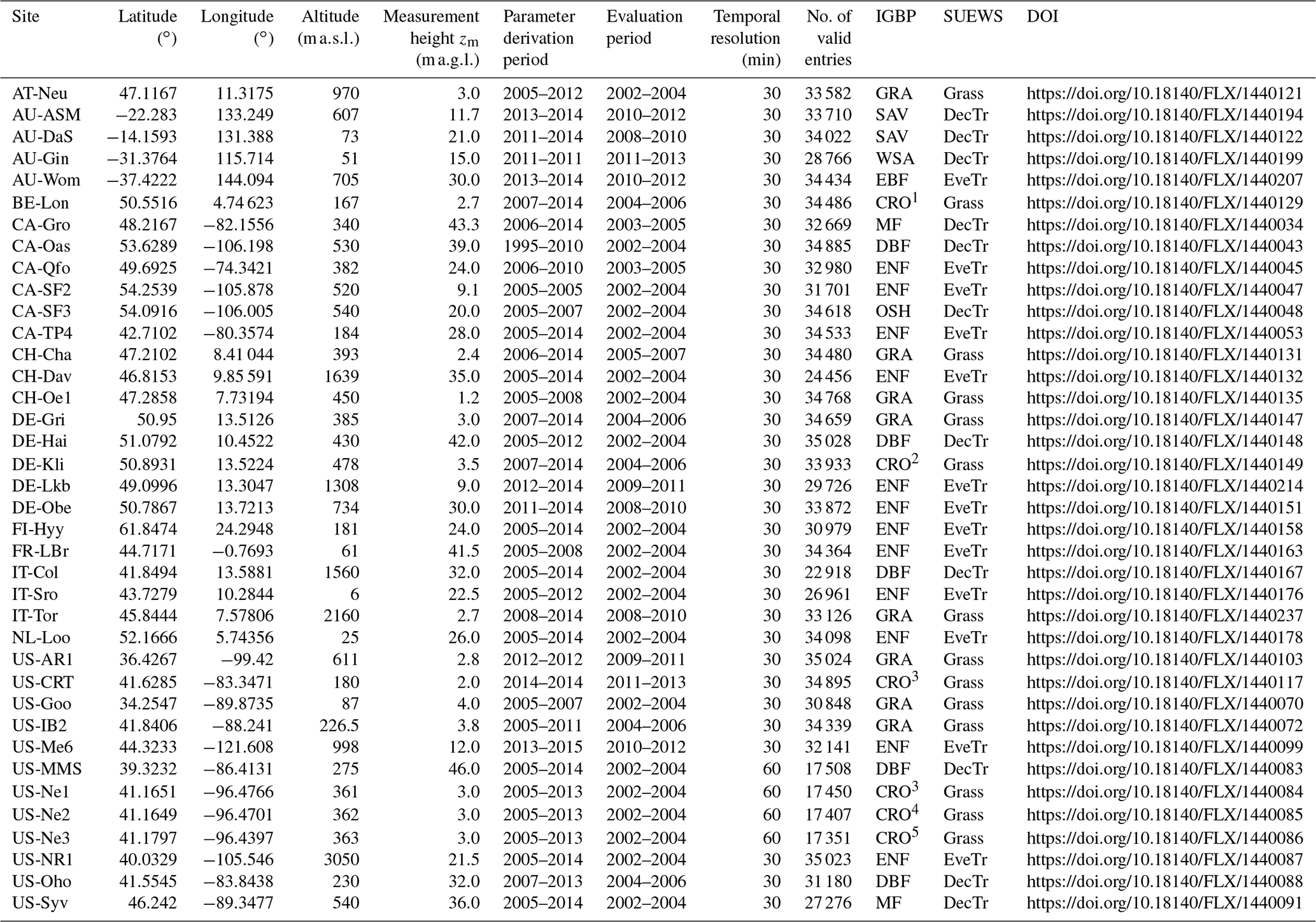
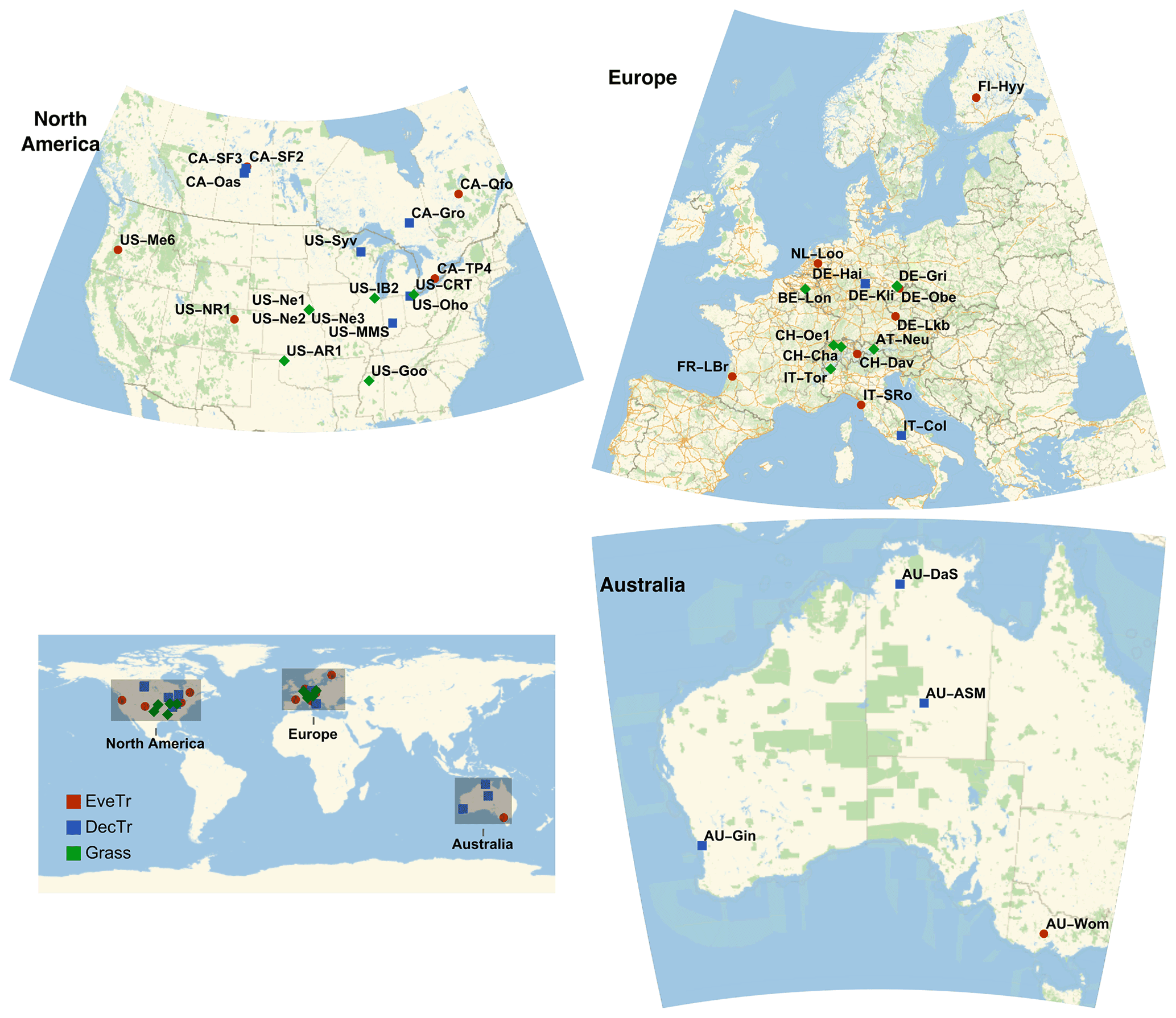
Figure 2 Location of FLUXNET sites (Table 3) coded by into three land cover types: deciduous trees (DecTr), evergreen trees (EveTr) and grass (Grass). Source of base map: © OpenStreetMap contributors, 2021. Distributed under the Open Data Commons Open Database License (ODbL) v1.0.

Half-hourly observations (Table 2) are used from 38 sites (Table 3) in three regions (Fig. 2). These sites are selected to meet the following criteria (number of remaining sites that met the criteria):

1. Sites with CC-BY 4.0 license (206/212).

2. Data availability (56/206). This requires both MODIS LAI data (available from 2002, Sect. 3.2) and long-term continuity (defined here as ≥ 3 years for the multiple needs).

3. Model capacity (38/56). The SUEWS v2020a LAI scheme is forced with only air temperature and not other variables (e.g. rainfall), which may strongly influence phenology at some sites (Appendix D). Hence, these sites are excluded.

Unfortunately, no datasets are left after selection based on the above criteria for some regions (Fig. 2), including Africa, Asia and South America.

As SUEWS allows any grid cell to have three vegetation or plant functional types (PFTs), with the sub-type or properties varying between grids, we subdivide the 38 sites into three classes using IGBP (Table 3) (code, number of sites):

• a.

  Evergreen trees/shrubs (EveTr, 13). Evergreen needleleaf forests (ENF, 12), evergreen broadleaf forests (EBF, 1).

• b.

  Deciduous trees/shrubs (DecTr, 11). Mixed forests (MF, 2), deciduous broadleaf forests (DBF, 5), open shrublands (OSH, 1), woody savannas (WSA, 1), savannas (SAV, 2).

• c.

  Grass (14). Grasslands (GRA, 8), croplands (CRO, 6).

The landscape heterogeneity of many FLUXNET EC flux measurements sites have been systematically examined by Stoy et al. (2013) using satellite imagery. Of the sites they examined, they found them to be located within homogeneous parts of the targeted PFT, but the larger landscape (∼ 20 km) may have considerable variability. As a FLUXNET site is typically assigned to one PFT for land surface model development and evaluation (e.g. Stöckli et al., 2008; Zhang et al., 2017; Chu et al., 2021), we configure each as a homogeneous grid cell and assume f_i=1.

3.2 MODIS LAI

The NASA Moderate Resolution Imaging Spectroradiometer (MODIS; Nishihama et al., 1997) four-day composite product MCD15A3H (Myneni et al., 2015) with 500 m resolution is treated as “observed” LAI. Product data are available from 2002. We use the Fixed Sites Subsetting and Visualization Tool (ORNL DAAC, 2018) for the FLUXNET dataset to extract the MCD15A3H time series. To obtain a daily time series we linearly interpolate between values, for parameter derivation (Sect. 4.1).

3.3 Soil information

The SoilGrids (Hengl et al., 2014) database provides soil properties (i.e. organic carbon, bulk density, cation exchange capacity (CEC), pH, soil texture fractions and coarse fragments) at seven depths (0, 0.05, 0.15, 0.30, 0.60, 1.00 and 2.00 m), as well as a bedrock depth prediction, World Reference Base (WRB) and USDA soil classes. We use the SoilGrids250m (Hengl et al., 2017) version, with its ∼ 280 raster layers, to obtain the parameters (Table 4) to derive soil moisture deficit at wilting point (Δθ_WP in mm) for soil-moisture-related calculations (e.g. Eq. 18).

Table 4 Soil-related parameters obtained from the SoilGrids (Hengl et al., 2014) database for each site (Table 3) at 250 m resolution for seven depths (Sect. 3.3). Values for each site (Table 3) are given in Sun et al. (2021).

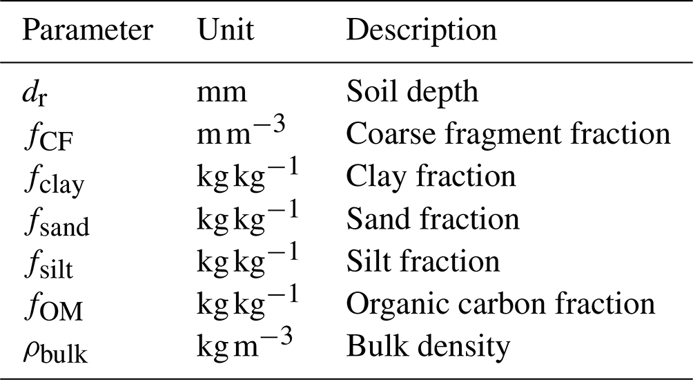
The difference in soil moisture between field capacity (θ_FC in mm) and wilting point (θ_WP in mm) are used with parameters defined as follows (Saxon and Rawls, 2006):

$$\begin{array}{}\text{(23)}& \mathrm{\Delta }{\mathit{\theta }}_{\text{WP}}={\mathit{\theta }}_{\text{FC}}-{\mathit{\theta }}_{\text{WP}}=(W_{\text{FC}}-W_{\text{WP}})(\mathrm{1}-f_{\text{CF}})d_{\mathrm{r}}\end{array}$$

with

$$\begin{array}{}\text{(24)}& W_{\text{FC}}=k_{\text{FC}}+\left(\mathrm{1.283}\cdot k_{\text{FC}}^{\mathrm{2}}-\mathrm{0.374}\cdot k_{\text{FC}}-\mathrm{0.015}\right),\end{array}$$

using the weight fractions of sand f_sand, clay f_clay and organic matter f_OM:

$$\begin{array}{}\text{(25)}& \begin{array}{rl}{k}_{\text{FC}}=& -\mathrm{0.251}\cdot f_{\text{sand}}+\mathrm{0.195}\cdot f_{\text{clay}}+\mathrm{0.011}\cdot f_{\text{OM}}\\ & +\mathrm{0.006}\cdot \left(f_{\text{sand}}{f}_{\text{OM}}\right)-\mathrm{0.027}\cdot \left(f_{\text{clay}}{f}_{\text{OM}}\right)\\ & +\mathrm{0.452}\cdot \left(f_{\text{sand}}{f}_{\text{clay}}\right)+\mathrm{0.299}\end{array}\end{array}$$

and

$$\begin{array}{}\text{(26)}& W_{\text{WP}}=k_{\text{WP}}+(\mathrm{0.14}\cdot k_{\text{WP}}-\mathrm{0.02}),\end{array}$$

where

$$\begin{array}{}\text{(27)}& \begin{array}{rl}{k}_{\text{WP}}=& -\mathrm{0.024}\cdot f_{\text{sand}}+\mathrm{0.487}\cdot f_{\text{clay}}+\mathrm{0.006}\cdot f_{\text{OM}}\\ & +\mathrm{0.005}\cdot \left(f_{\text{sand}}{f}_{\text{OM}}\right)-\mathrm{0.013}\cdot \left(f_{\text{clay}}{f}_{\text{OM}}\right)\\ & +\mathrm{0.068}\cdot \left(f_{\text{sand}}{f}_{\text{clay}}\right)+\mathrm{0.031}.\end{array}\end{array}$$

4 Parameter derivation for vegetated land covers: workflows and results

4.1 Leaf area index (LAI) and albedo-related parameters

LAI is a key phenology parameter in SUEWS; it moderates albedo (α) and therefore surface radiative exchanges. LAI changes also modify both aerodynamic roughness parameters (roughness length z₀, zero plane displacement height z_d) (e.g. Kent et al., 2017a, b) impacting aerodynamic resistance (r_a) and surface resistance (r_s). LAI directly moderates Q_E and canopy interception capacity, which modifies when potential evaporation occurs and aspects of the water balance.

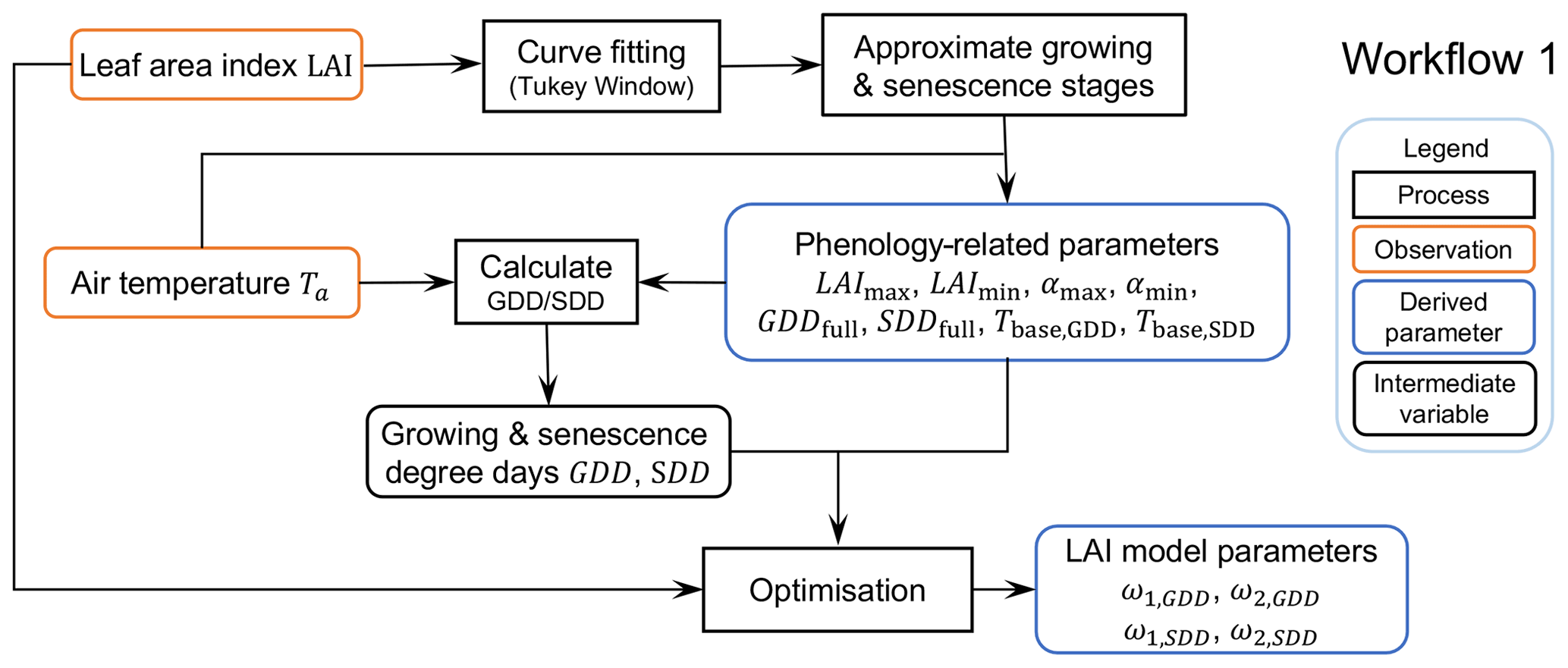
Figure 3 Workflow 1 (Fig. 1) for deriving LAI- and albedo-related parameters. Related Jupyter notebooks are provided in Sun et al. (2021).

As the SUEWS LAI equation (Eq. 4) makes global optimisation techniques numerically challenging to derive all the required parameters, we take a two-step approach (Fig. 3).

4.1.1 Approximating growing stages using an asymmetric Tukey window function

The Tukey or cosine-tapered window (TW) is used in signal processing applications when data need to be processed in short segments. It is defined as follows (Bloomfield, 2000):

$$\begin{array}{}\text{(28)}& \begin{array}{rl}& \text{TW}(x,a)=\\ & \left\{\begin{array}{ll}\mathrm{1}& (\mathrm{0}<a<\mathrm{1}\wedge a-\mathrm{2}x-\mathrm{1}\\ & \le \mathrm{0}\wedge a+\mathrm{2}x-\mathrm{1}\le \mathrm{0})\\ & \vee (a=\mathrm{1}\wedge x=\mathrm{0})\\ & \vee \left(a\le \mathrm{0}\wedge -\frac{\mathrm{1}}{\mathrm{2}}\le x\le \frac{\mathrm{1}}{\mathrm{2}}\right)\\ \frac{\mathrm{1}}{\mathrm{2}}\left(\cos \right(\mathrm{2}\mathit{\pi }x)+\mathrm{1})& a>\mathrm{1}\wedge -\frac{\mathrm{1}}{\mathrm{2}}\le x\le \frac{\mathrm{1}}{\mathrm{2}}\\ \frac{\mathrm{1}}{\mathrm{2}}\left(\cos \left(\frac{\mathrm{2}\mathit{\pi }\left(-\frac{a}{\mathrm{2}}+x+\frac{\mathrm{1}}{\mathrm{2}}\right)}{a}\right)+\mathrm{1}\right)& \mathrm{0}<a\le \mathrm{1}\wedge x\ge -\frac{\mathrm{1}}{\mathrm{2}}\wedge a\\ & -\mathrm{2}x-\mathrm{1}>\mathrm{0}\\ \frac{\mathrm{1}}{\mathrm{2}}\left(\cos \left(\frac{\mathrm{2}\mathit{\pi }\left(\frac{a}{\mathrm{2}}+x-\frac{\mathrm{1}}{\mathrm{2}}\right)}{a}\right)+\mathrm{1}\right)& \mathrm{0}<a\le \mathrm{1}\wedge a+\mathrm{2}x-\mathrm{1}\\ & >\mathrm{0}\wedge x\le \frac{\mathrm{1}}{\mathrm{2}}\\ \mathrm{0}& \mathrm{|}x\mathrm{|}>\frac{\mathrm{1}}{\mathrm{2}},\end{array}\right.\end{array}\end{array}$$

where x is the independent variable and a is the curve shape factor. We propose an asymmetric form of the Tukey window (aTW) to approximate the intra-annual LAI dynamics:

$$\begin{array}{}\text{(29)}& \text{aTW}(x,a,b,x_{\mathrm{0}},l)=\left\{\begin{array}{ll}\text{TW}\left(\frac{x-x_{\mathrm{0}}}{l},a\right)& x<x_{\mathrm{0}},\\ \text{TW}\left(\frac{x-x_{\mathrm{0}}}{l},b\right)& x\ge x_{\mathrm{0}},\end{array}\right.\end{array}$$

where b is a curve shape factor for different segments, x₀ the segment parameter and l the rescaling factor.

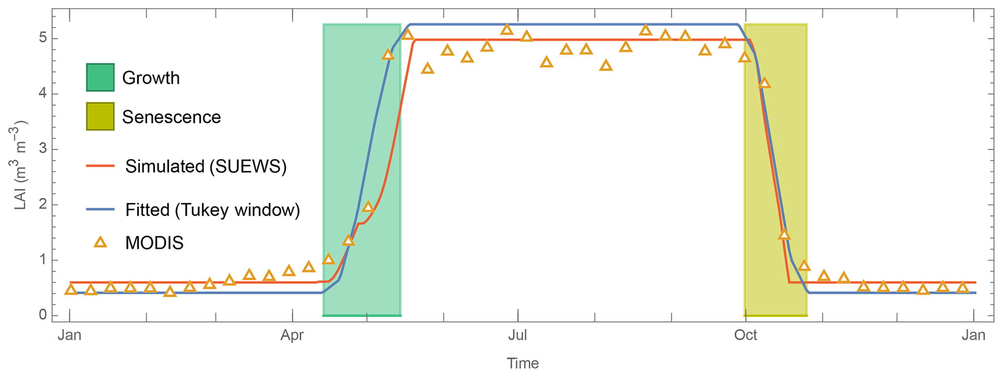
Figure 4 Intra-annual LAI dynamics at US-MMS multi-year (2002–2014) ensemble median derived from MODIS observations (open triangle, Sect. 3.2) and simulated by SUEWS temperature-based LAI scheme (Eq. 4) (orange line) with Tukey window fit (blue line, Sect. 4.1) using to derive the leaf-on or growth period (green shading) and senescence (yellow shading) periods.

To demonstrate this we use the US-MMS site (Table 3), to fit the intra-annual LAI dynamics using an aTW curve (blue line, Fig. 4) to determine different phenological stages (shading, Fig. 4) and subsequently derive several related parameters:

• LAI_min. 5th percentile of LAI values before the growth and after the senescence.

• LAI_max. 75th percentile of LAI values after the growth and before the senescence.

• T_base,GDD. 99th percentile of air temperatures before the growth.

• T_base,SDD. 10th percentile of air temperature after the growth and before the senescence.

• GDD_full. GDD at the end of growth based on T_base,GDD.

• SDD_full. SDD at the end of senescence based on T_base,SDD.

• α_min/α_max. 10th/90th percentile of daily albedo values after the growth and before the senescence. A daily albedo is calculated from 30 or 60 min FLUXNET observations of incoming and outgoing shortwave radiation for the period 10:00 to 14:00 LST (local standard time). To remove outliers a clustering method is applied (ClusterClassify of Mathematica v12.3.1, Wolfram Research, 2020). For example, at some high-latitude sites (e.g. CA-Oas) snow occurs, the winter values are based on data from shortly after senescence to shortly before growth (next spring) and the clustering approach removes the snow period albedo values.

For evergreen and deciduous trees, ${\mathit{\alpha }}_{\text{LAI},min}$ (${\mathit{\alpha }}_{\text{LAI},max}$) in Eq. (6) typically corresponds to α_min (α_max), while for grassland a reverse relation holds (i.e. ${\mathit{\alpha }}_{\text{LAI},min}$ corresponds to α_max and vice versa; see Cescatti et al., 2012, for a detailed analysis of albedo dynamics at FLUXNET sites).

4.1.2 Deriving curve factors used in SUEWS LAI scheme

With the parameters derived in step 1, we can determine the curve factors ${\mathit{\omega }}_{\mathrm{1}/\mathrm{2},\text{GDD}/\text{SDD}}$ by minimising the bias between MODIS observed (open triangle, Fig. 4) and SUEWS-simulated (red line, Fig. 4) LAI values.

Table 5 Inter-site variability within the three vegetation classes of LAI- and albedo-related parameters (Eq. 4, Sect. 4.1) shown by mean and standard deviation. For individual site and PFT parameters see Appendix C (for digital version see Sun et al., 2021). Median and interquartile range (IQR) see Fig. 5.

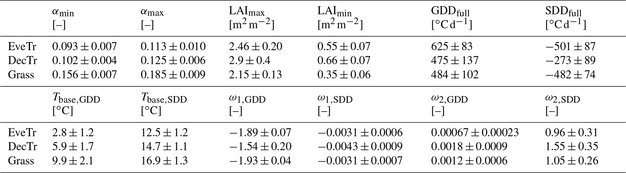
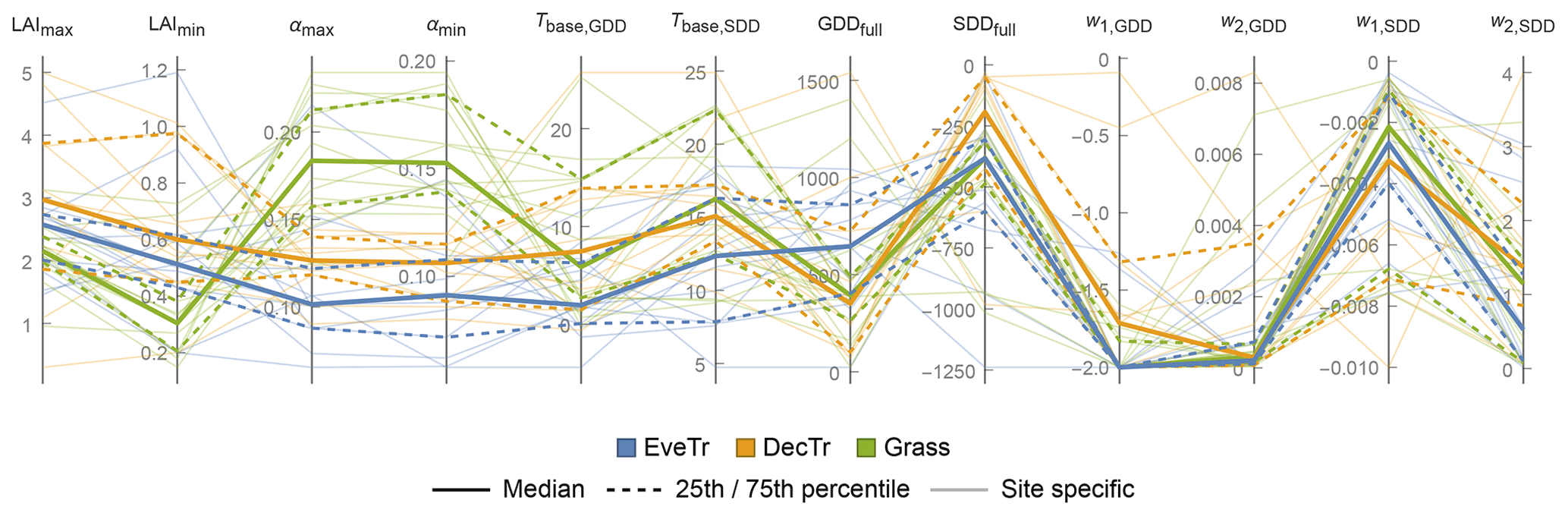
Figure 5 Variation in LAI-related parameters (12 labelled vertical lines, Sect. 2.2.1) within three land cover classes (colour) showing median (thick line), interquartile range (IQR, 25th and 75th percentiles, dashed lines) and site-specific values (thin lines).

The derived LAI-related parameters for the 38 FLUXNET sites vary between different land cover groups (Table 5, Fig. 5). The derived ${\text{LAI}}_{max/min}$ results are consistent with those reported in the literature (Asaadi et al., 2018). For EveTr sites, the large contrast between LAI_max and LAI_min in the ENF sites analysed here is consistent with MODIS derived LAI for ENF, which has larger seasonal variability than EBF (Heiskanen et al., 2012), but some of this is caused by a known issue of particularly low winter values (Garrigues et al., 2008).

Given the global availability of MODIS LAI and reanalysis-based air temperature datasets, we suggest the LAI-related parameters be derived following this workflow (Fig. 3) to set parameters for SUEWS simulations. This can be done independent of the availability of flux tower observations.

4.2 Storage heat flux coefficients

To calculate the storage heat flux ΔQ_S, the required OHM coefficients (Eq. 7) can be determined from observed net all-wave radiation and observed storage heat flux, using ordinary linear regression. As the FLUXNET sites chosen are considered to be homogeneous, we derive coefficients for each site.

Ideally the storage heat flux measurements would include each of the components that are heating and cooling down on a daily basis, such as the soil, trunk, branches, leaves and air volume in a forest (e.g. McCaughey et al., 1985; Oliphant et al., 2004). However, these measurements are unavailable in the FLUXNET2015 dataset. Hence, we calculate a residual flux $\mathrm{\Delta }{Q}_{\mathrm{S},\text{res}}=Q^{\ast }-(Q_{\mathrm{H}}+Q_{\mathrm{E}})$ by assuming energy balance closure. This has the problem of accumulating the net measurement errors in this term (Grimmond et al., 1991; Grimmond and Oke, 1999).

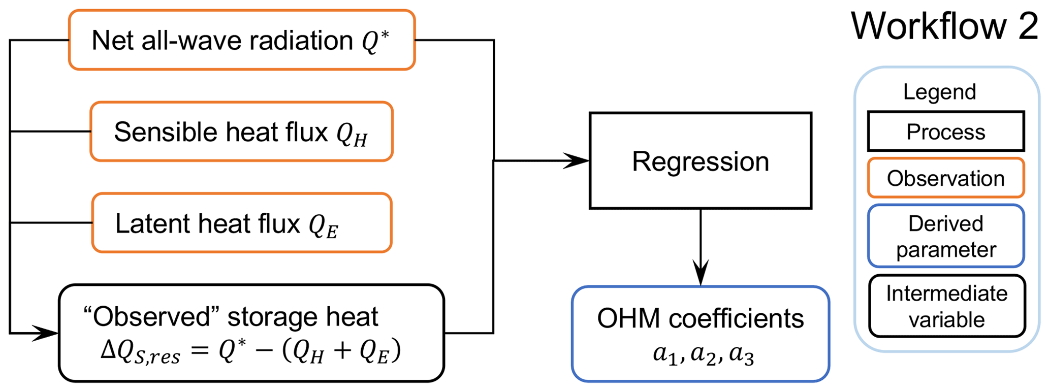
Figure 6 Workflow 2 (Fig. 1) to derive OHM coefficients. Related notebooks are provided in Sun et al. (2021).

The derived OHM coefficients (Fig. 6) can be determined by season (Anandakumar, 1999; Ward et al., 2016; Sun et al., 2017). We distinguish warm (“summer”) and cold (“winter”) seasons using months (summer: Northern Hemisphere JJA; Southern Hemisphere: DJF; winter: DJF (JJA), respectively). For simplicity, we omit periods when LAI may be changing rapidly. If the daily mean air temperature is warmer (cooler) than the annual mean of daily median temperature, then summer (winter) OHM coefficients are used in the simulations.

Table 6 As Table 5, but for OHM-related parameters (Sect. 4.2). See Fig. 7 for comparison and Table C2 for site-specific values.

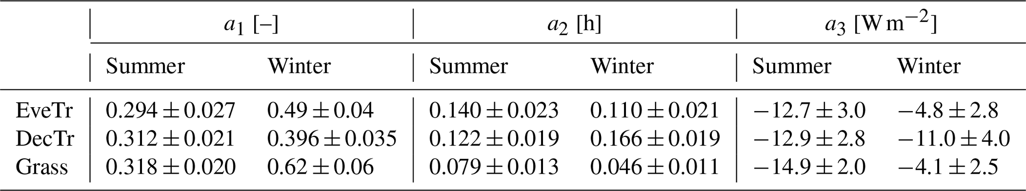
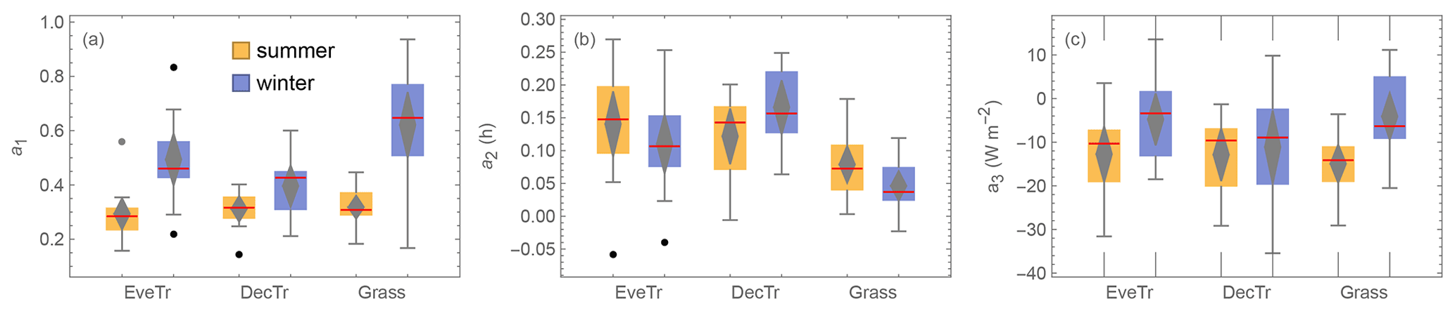
Figure 7 Boxplots showing variability of OHM coefficients between land covers (EveTr, DecTr and Grass) and seasons (summer and winter): (a) a₁ (b) a₂ and (c) a₃. Boxes (25th and 75th percentiles) and whiskers (5th and 95th percentiles), with median (red line) and mean (middle grey diamond, with 95 % confidence level (top and bottom) values, and outliers (dots).

The OHM coefficients derived for the 38 FLUXNET sites (Table 6, Fig. 7) vary between land cover types and seasons. For each land cover type, a₁ and a₃ are notably larger in winter than in summer while the seasonal difference in a₂ is relatively small. Thus the overall fraction of heat stored does not vary much, but the diurnal hysteresis effect is weaker in winter. These results are consistent with previous analytical results (Sun et al., 2017). Within each PFT, there is larger variability in a₂ and a₃ (cf. a₁), notably for evergreen and deciduous trees, suggesting using the most appropriate site values (e.g. medians) may improve predictions of the storage heat flux. In addition to the values derived here, we note that more detailed ΔQ_S observations are available for vegetated sites to derive such OHM coefficients (e.g. McCaughey, 1985; Oliphant et al., 2004).

4.3 Surface-conductance-related parameters

As the Jarvis-type formulation of stomatal and surface conductance is widely used for many land cover types, many parameter sets exist (e.g. Stewart, 1988; Grimmond and Oke, 1991; Ogink-Hendriks, 1995; Wright et al., 1995; Bosveld and Bouten, 2001; Järvi et al., 2011). Hoshika et al.'s (2018) comprehensive meta-analysis of published Jarvis-type stomatal conductance parameter values includes major woody and crop plants broadly similar to PFTs examined here.

Conventionally, the surface conductance parameters are derived by minimising the bias between the parameterised (Eq. 14) and so-called “observed” values derived from an inverse form of the Penman–Monteith equation (Eq. 3):

$$\begin{array}{}\text{(30)}& {\displaystyle \frac{\mathrm{1}}{g_{\mathrm{s}}}}=r_{\mathrm{s}}=\left[{\displaystyle \frac{s}{\mathit{\gamma }}}{\displaystyle \frac{Q_{\mathrm{H}}}{Q_{\mathrm{E}}}}-\mathrm{1}\right]r_{\mathrm{a}}+{\displaystyle \frac{\mathit{\rho }{c}_{\mathrm{p}}\text{VPD}}{\mathit{\gamma }{Q}_{\mathrm{E}}}}.\end{array}$$

This requires the surface be dry (Sect. 2.2.4) which we define as being without recorded rainfall in 24 h.

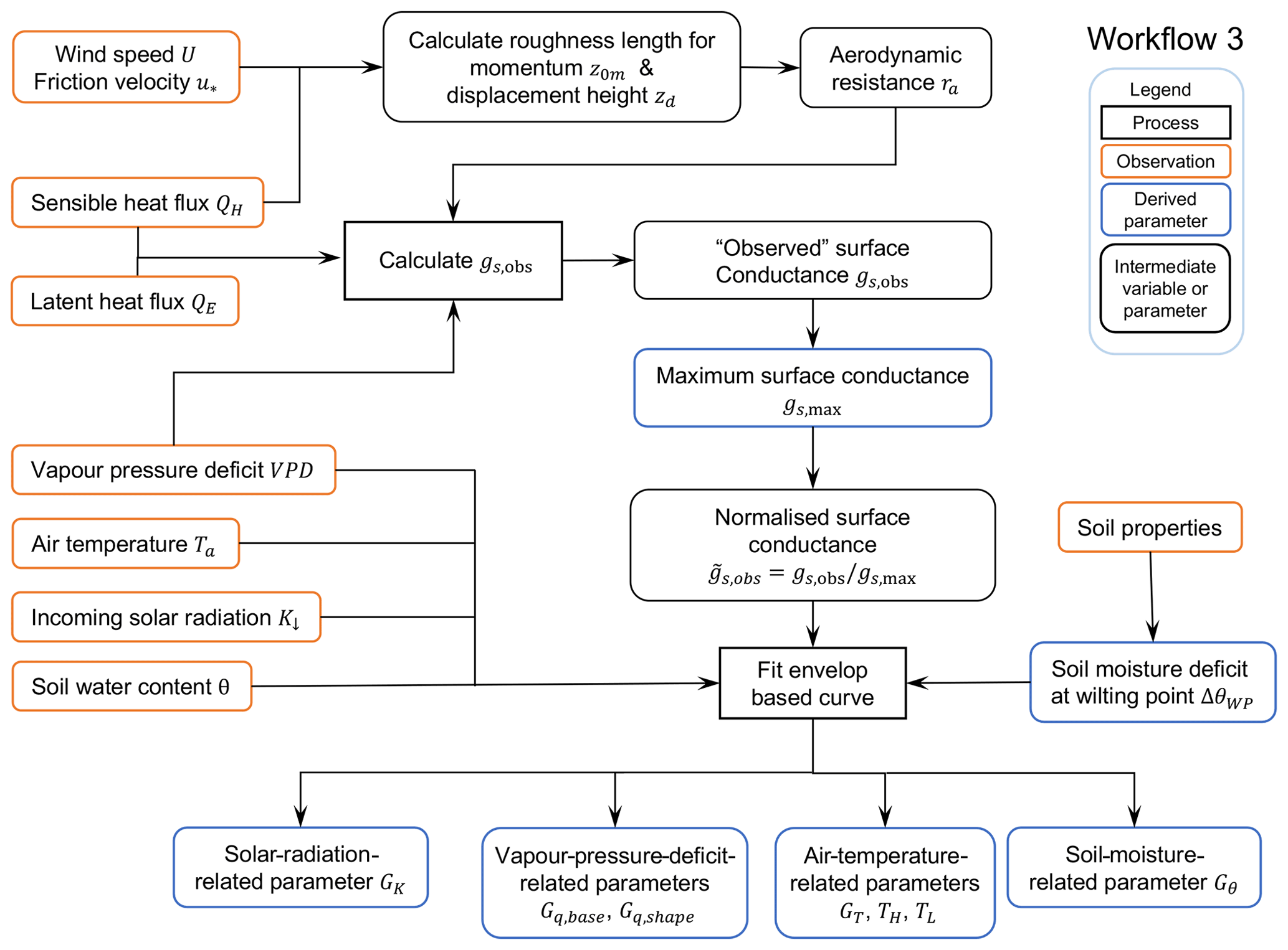
Figure 8 Workflow 3 (Fig. 1) for deriving surface-conductance-related parameters. Related notebooks are provided in Sun et al. (2021).

However, as the optimisation may not return values because of the complexity in Eq. (13) and the challenge of interpreting the derived parameter values, we adopt Matsumoto et al.'s (2008) approach to derive these parameters. Rather than using all the data combinations for g_s, the upper boundary of each forcing variable component (e.g. g(K_↓)) is considered as the response for unconstrained conditions. Specifically, the workflow is as follows (Fig. 8):

1. Calculate aerodynamic resistance r_a (Eq. 8) with roughness length z_0m and displacement height z_d derived from observed wind speed under neutral conditions (Appendix B).

2. Calculate “observed” surface conductance g_s,obs (Eq. 30)​​​​​​​.

3. Remove outliers from g_s,obs data (step 2) iteratively (i.e. values larger than the 98th percentile until difference between 98th and 99th percentiles is < 1 mm s⁻¹). The remainder are used for deriving parameters.

4. Determine the upper boundaries of g_s curves with each component variable. To demonstrate this we use the US-MMS site (Fig. 9). First, original data are binned (sizes: 50 W m⁻² for K_↓, 2 ^∘C for T_a, 2 kg kg⁻¹ for Δq and 10 mm for Δθ), the 95th percentiles of these bins are sampled 100 times (bootstrapped) to determine anchor points (red dots, Fig. 9). Second, the parameters are fit to the g_s related curves (Eqs. 14–17) using the anchor points using NonlinearModelFit of Mathematica v12.3.1 (Wolfram Research, 2008).

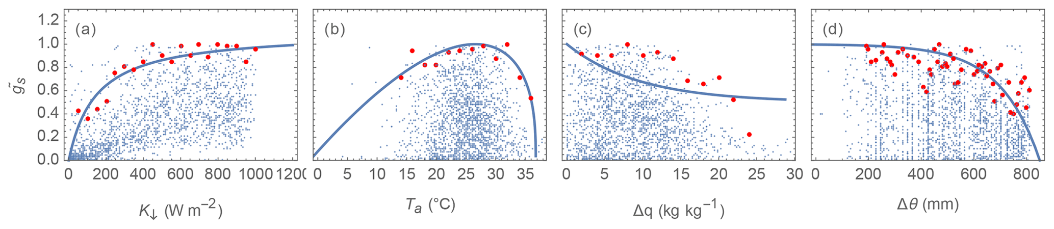
Figure 9 Derived relations (blue lines) between normalised surface conductance ${\stackrel{\mathrm{̃}}{g}}_{\mathrm{s}}$ and (a) incoming solar radiation K_↓, (b) air temperature T_a, (c) specific humidity deficit Δq, and (d) soil moisture deficit Δθ based on anchor data points (red dots) after bootstrapping of observations (blue dots) for an example site (US-MMS).

Table 7 As Table 5, but for surface-conductance-related parameters (Sect. 4.3). See Fig. 10 and Appendix C.

Figure 10 As Fig.5, but for surface-conductance-related parameters.

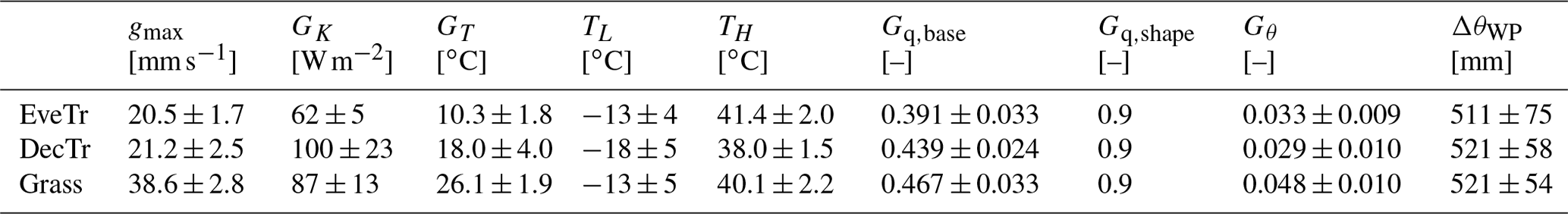
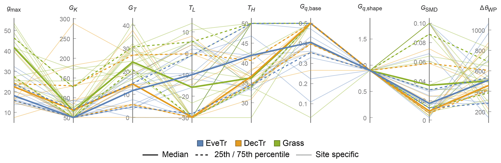
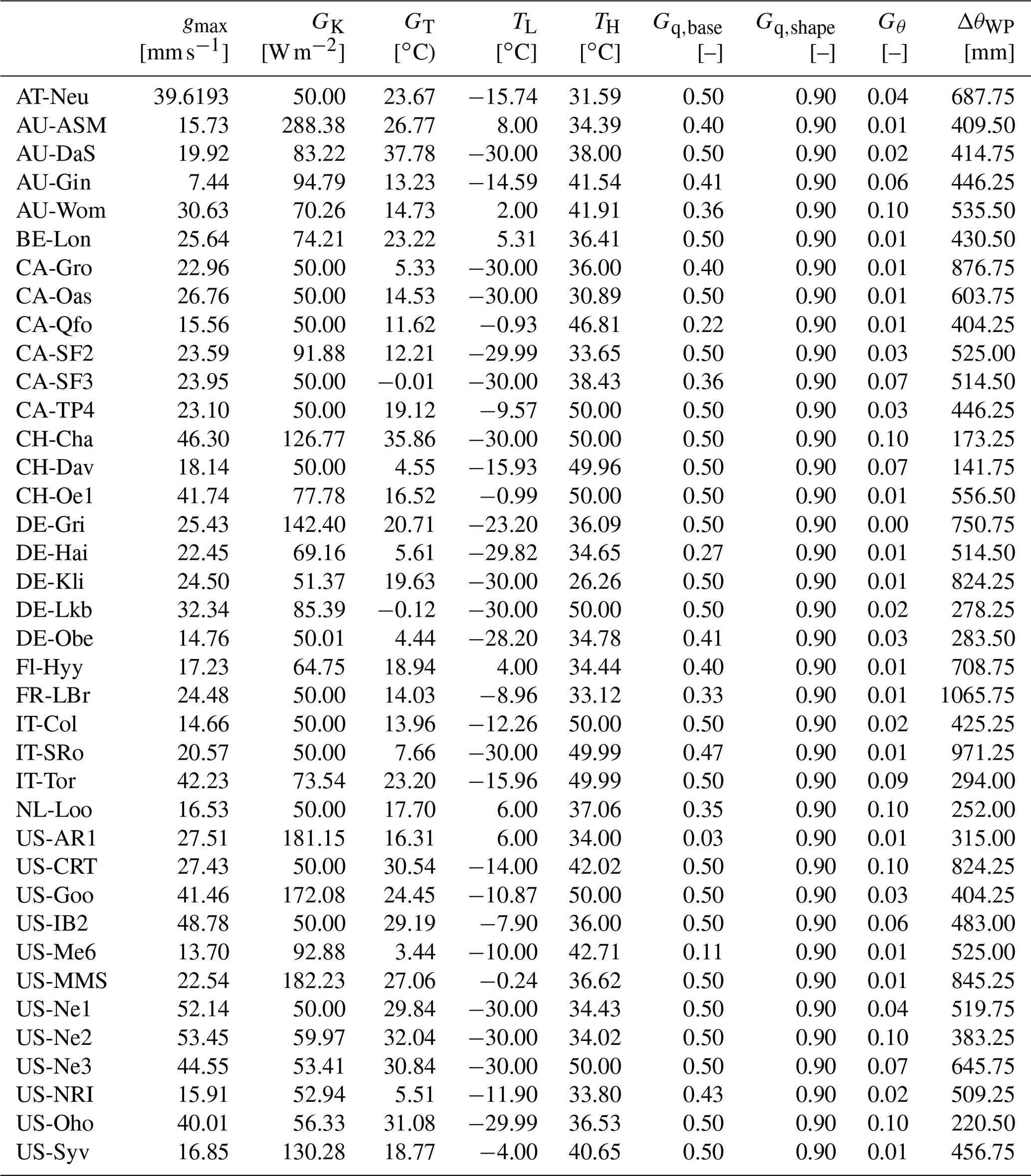
The derived surface conductance parameters for the 38 FLUXNET sites (Tables 7 and C3) have different intra-PFT variability based on the IQR (dotted lines, Fig. 10) and demonstrates the benefit of the observations and of deriving site values when possible. It may help in selecting appropriate PFTs from other sources (e.g. NOAH values in Appendix A). The g_max results are consistent with Hoshika et al. (2018) in terms of inter-PFT ordering (Grass > EveTr and DecTr). The grass and crop values are comparable (Table C3) to Hoshika et al. (2018); however, our derived deciduous trees values are smaller (22 vs. 31 mm s⁻¹) and evergreen trees values larger (20 vs. 12 mm s⁻¹).

A consistent G_q,shape (Eq. 16) value (0.9 units) is obtained for all sites, implying potential for improvements to the g(Δq) relation between g_s and Δq (e.g. other formulations g_s(Δq) in Matsumoto et al., 2008) in future SUEWS development. This would be beneficial as there is a clear “plateau” observed for low Δq (Fig. 9c). Similar issues are found in g(Δθ) for soil-moisture-related parameters. Although the parameters derived here are the “best” fit to the g_s forms in SUEWS v2020a, for each component variable multiple g_s formulations exist with a range of variable fitting performance (e.g. Fig. A1 in Ward et al., 2016). Here, we focus on deriving the parameters rather than proposing new or more appropriate formulations.

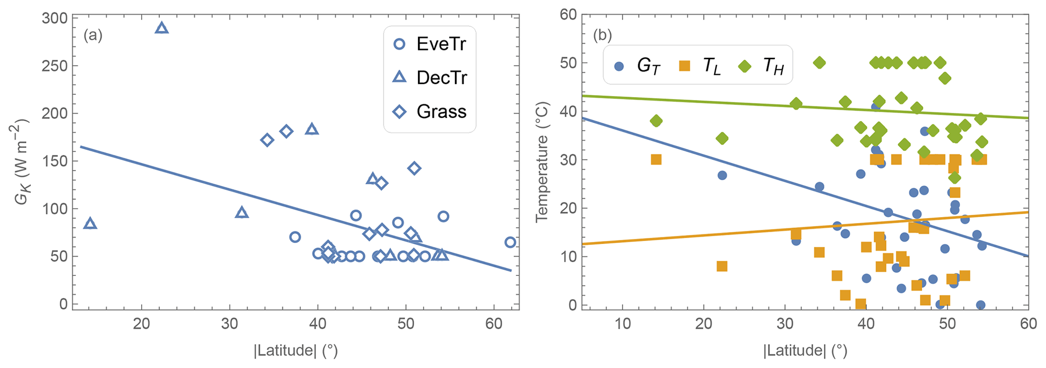
Figure 11 Relations between absolute latitude and derived parameters: (a) solar-radiation-related G_K by PFT (symbol) and (b) temperature-related G_T, T_L and T_H. Lines are derived by ordinary linear regression. See text for notation definitions.

The solar-radiation-related G_K parameter is linked to the level of incoming solar radiation needed for evapotranspiration to occur. Given incoming solar radiation intensity varies with latitude, we see G_K generally decreases polewards (Fig. 11a), suggesting geographical location could be used as a proxy for deriving G_K.

The air-temperature-related G_T parameter indicates the optimal temperature for evapotranspiration to reach its probable maxima. G_T appears to have a negative relation with latitude, but the two other temperature parameters (T_L and T_H) have a very weak (or no) relation with latitude (Fig. 11b). This suggests a universal temperature range between T_L and T_H might be applicable across different sites while G_T should be determined on a site-by-site basis.

5 SUEWS performance in vegetated areas

5.1 SUEWS configuration and evaluation

SUEWS v2020a (Tang et al., 2021) is evaluated using its Python wrapper SuPy v2021.3.18 (Sun and Grimmond, 2019) with parameters (Table 1) and gap-filled 30 or 60 min meteorological forcing data (Table 2) based on FLUXNET2015 dataset. Simulations are conducted, with forcing data interpolated to a 5 min time step (Ward et al., 2016), for 3 years (Table 3, Evaluation period) starting in mid-winter. The first year is discarded to allow for model spin-up. The two subsequent years are evaluated when observed latent heat flux data are available. In these model runs, the z_0m and z_dm values used are derived (Appendix B) by LAI state using observations for each LAI season (approximately nine values per site; see Sun et al. (2021) for values). All other parameters (Table 1) are determined for the parameter derivation period indicated in Table 3. At one site (AU-Gin), there are insufficient data for independent evaluation period from the parameter derivation period.

For the periods with 30 or 60 min Q_E EC observations (Y_obs) available, the 5 min simulated values (Y_mod) are averaged to 30 or 60 min to evaluate the j cases between 1 and the number of data points (N). The following metrics are used:

1. Hit rate (HR).

   $$\begin{array}{}\text{(31)}& \text{HR}={\displaystyle \frac{{\sum }_{j=\mathrm{1}}^{N}H({\mathit{\delta }}_{Y,j}-\mathrm{|}{Y}_{\text{mod},j}-Y_{\text{obs},j}\mathrm{|})}{N}},\end{array}$$

   with Heaviside step function H defined by

   $$\begin{array}{}\text{(32)}& H\left(x\right)=\left\{\begin{array}{ll}\mathrm{0},& x<\mathrm{0},\\ \mathrm{1},& x\ge \mathrm{0},\end{array}\right.\end{array}$$

   and the threshold δ_Y,jbeing a value dependent on evaluation variable Y.

   In particular, δ_Y,j for Q_E is determined as a function of net all-wave radiation Q^∗ following Hollinger and Richardson (2005) to be ${\mathit{\delta }}_{Y,j}=\mathrm{0.1}{Q}_j^{\ast }+\mathrm{10}$ (in W m⁻²) based on measurement uncertainties.

2. Mean absolute error (MAE).

   $$\begin{array}{}\text{(33)}& \text{MAE}={\displaystyle \frac{{\sum }_{j=\mathrm{1}}^N\mathrm{|}{Y}_{\text{mod},j}-Y_{\text{obs},j}\mathrm{|}}{N}}\end{array}$$

3. Mean bias error (MBE).

   $$\begin{array}{}\text{(34)}& \text{MBE}={\displaystyle \frac{{\sum }_{j=\mathrm{1}}^N(Y_{\text{mod},j}-Y_{\text{obs},j})}{N}}\end{array}$$

Both the MAE and MBE would ideally be 0 (with units of parameter and variable assessed), whereas if the HR = 1 it indicates all model predictions fall within the acceptable threshold set, while HR = 0 would suggest none are within the acceptance threshold.

A performance score PS as a function for each metric (x; i.e. HR, MAE, |MBE|) is used to rank the sites:

$$\begin{array}{}\text{(35)}& \text{PS}={\displaystyle \frac{\mathrm{1}}{N}}{\sum }_{k=\mathrm{1}}^N(w_x\stackrel{\mathrm{̃}}{x}{)}_k,\end{array}$$

where $\stackrel{\mathrm{̃}}{x}$ is the rescaled ranking score of a given metric after being ranked from poorest to best, and w_x is a weight associated with the temporal analysis type k which varies from 1 to N (number of component periods; e.g. N = 24 for hourly results). Equal weights ($\mathrm{1}/\mathrm{3}$) are used in the PS calculations for HR, MAE and |MBE|.

5.2 Impacts of model parameters on model performance

Given the many parameters in SUEWS, first we assess the relative importance of the parameters. We assume in this analysis our derived parameters (Sect. 4) are “perfect”, so we can undertake a sensitivity analysis (McCuen, 1974; Beven, 1979) of the Penman–Monteith equation (i.e. Eq. 3, denoted by PM hereafter):

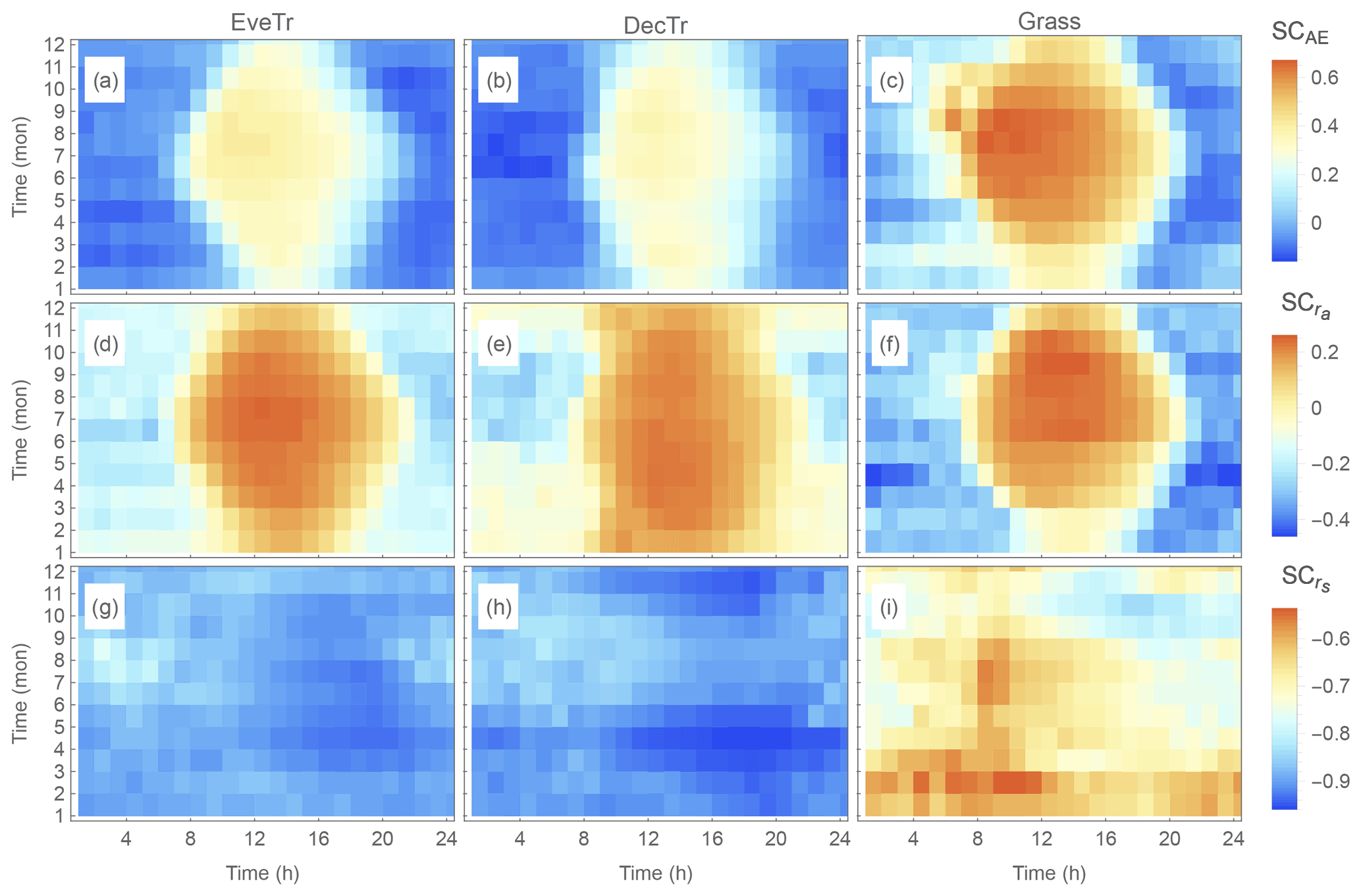
Figure 12 Temporal variation in median (colour) sensitivity coefficient (SC, Eq. 38​​​​​​​) of (a–c) available energy (AE, Sect. 5.1), (d–f) aerodynamic resistance (r_a) and (g–i) surface resistance (r_s) for (a, d and g) evergreen trees (EveTr), (b, e and h) deciduous trees (DecTr), and (c, f and i) grassland and crops (Grass).

$$\begin{array}{}\text{(36)}& \mathrm{\Delta }{Q}_{\mathrm{E}}=\text{PM}(\text{AE}+\mathrm{\Delta }\text{AE},r_{\mathrm{a}}+\mathrm{\Delta }{r}_{\mathrm{a}},r_{\mathrm{s}}+\mathrm{\Delta }{r}_{\mathrm{s}})-Q_{\mathrm{E}},\end{array}$$

where $\text{AE}=Q^{\ast }-\mathrm{\Delta }{Q}_{\mathrm{S}}$ is the available energy, incorporating parameter influences related to LAI, albedo and OHM. Similarly, multiple parameters influence the resistance terms. In Eq. (36)​​​​​​​ the prefix Δ indicates bias terms. For simplicity, we consider the direct impacts only (i.e. secondary impacts from parameters inter-dependence are ignored). Expanding Eq. (36) in Taylor series, gives the following:

$$\begin{array}{}\text{(37)}& \mathrm{\Delta }{Q}_{\mathrm{E}}\approx {\text{PM}}^{\prime }\left(\text{AE}\right)\cdot \mathrm{\Delta }\text{AE}+{\text{PM}}^{\prime }\left(r_{\mathrm{a}}\right)\cdot \mathrm{\Delta }{r}_{\mathrm{a}}+{\text{PM}}^{\prime }\left(r_{\mathrm{s}}\right)\cdot \mathrm{\Delta }{r}_{\mathrm{s}},\end{array}$$

where PM^′(x), the first-order derivative of x, indicates the sensitivity of modelled Q_E. Note “≈” implies the approximation of ΔQ_E as the sum of bias from the chosen parameters. To examine the influences of different parameters in model performance, we use two non-dimensional metrics derived from Eq. (37):

1. Sensitivity coefficient (SC) (McCuen, 1974).

   $$\begin{array}{}\text{(38)}& \text{SC}={\text{PM}}^{\prime }\left(x\right)\cdot {\displaystyle \frac{x}{Q_{\mathrm{E}}}}={\displaystyle \frac{\partial Q_{\mathrm{E}}}{\partial x}}{\displaystyle \frac{x}{Q_{\mathrm{E}}}}\approx {\displaystyle \frac{\mathrm{\Delta }{Q}_{\mathrm{E}}/Q_{\mathrm{E}}}{\mathrm{\Delta }x/x}}\end{array}$$

   gives the fractional change in x causing a change in Q_E, indicating a relative sensitivity of PM to x. For instance, SC = 0.5 suggests a 20 % increase in x may increase Q_E by 10 % (= 20 % × 0.5).

2. Attribution fraction (AF). quantifies the fraction of model bias derived from a given parameter x:

   $$\begin{array}{}\text{(39)}& \text{AF}={\text{PM}}^{\prime }\left(x\right)\cdot {\displaystyle \frac{\mathrm{\Delta }x}{\mathrm{\Delta }{Q}_{\mathrm{E}}}}.\end{array}$$

Ideally, the sum of all AF contributors would equal 1, but as we omit inter-dependence of impacts of parameters, this may not occur. However, comparing the different contributors is indicative of their relative importance in modelled Q_E.

Both SC_AE and ${\text{SC}}_{r_{\mathrm{a}}}$ generally show a similar type of pattern (Fig. 12a–f) with seasonal and diurnal variations for the three PFTs. During warm periods (summer and noon), with an increase in ΔAE and Δr_a it is found to lead to larger positive bias in modelled Q_E, whereas in cooler periods (winter and night-time) the ΔAE and Δr_a is found to increase the negative bias.

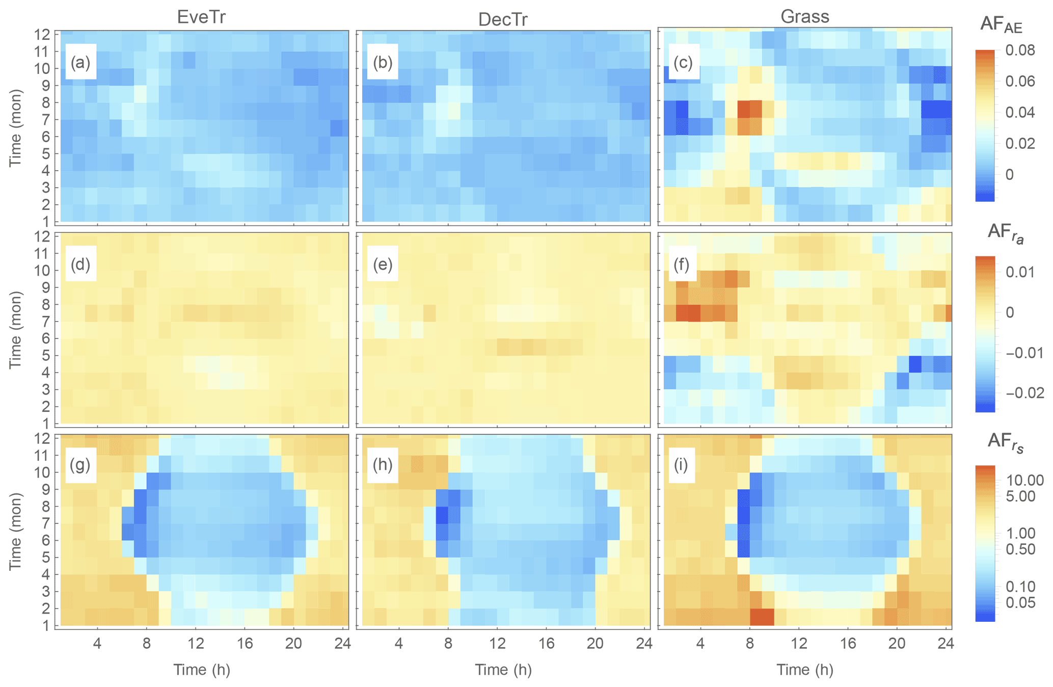
Figure 13 As Fig.12, but the attribution fraction (AF, Eq. 39). Note AF_rs scale is logarithmic.​​​​​​​

However, the temporal patterns in ${\text{SC}}_{r_{\mathrm{s}}}$ differ (Fig. 13g–i) from those in SC_AE (Fig. 13a–c) and ${\text{SC}}_{r_{\mathrm{a}}}$ (Fig. 13d–f): the ${\text{SC}}_{r_{\mathrm{s}}}$ values are always negative, and consistently larger in magnitude (cf. SC_AE and ${\text{SC}}_{r_{\mathrm{a}}}$), implying a particularly strong sensitivity of Q_E to r_s. This is consistent with Beven (1979), who found it to dominate the modelled summertime Q_E sensitivity in the PM framework.

The relative (cf. total) bias from the parameters is assessed in modelled Q_E at monthly and hourly temporal scales using the median AF (Fig. 13). ${\text{AF}}_{r_{\mathrm{s}}}$ is larger than both AF_AE and ${\text{AF}}_{r_{\mathrm{a}}}$; i.e. r_s imposes a dominant influence in modelled Q_E bias. There is more temporal variability in ${\text{AF}}_{r_{\mathrm{s}}}$ (cf. AF_AEand ${\text{AF}}_{r_{\mathrm{a}}}$) with cooler periods (morning and evening, whole winter) generally having values greater than 1, indicating the bias in r_s dominates modelled Q_E. As ${\text{AF}}_{r_{\mathrm{s}}}$ is still generally larger than ∼ 0.3 (except for transitional periods in summer, 08:00–09:00 LST, when ${\text{AF}}_{r_{\mathrm{s}}}\mathit{\lesssim }\mathrm{0.3}$), r_s remains an important control on modelled Q_E. These results together indicate that it is critical to assign accurate r_s to obtain accurate estimates of Q_E.

5.3 Evaluation of SUEWS-simulated Q_E with two different sources of g_s parameters

Given the critical importance of surface resistance to model performance in Q_E (Sect. 5.2), we assess the impact of two different sources of g_s parameters (keeping all other site parameters the same, with the values as indicated in Sect. 5.1): (i) site-specific values derived from FLUXNET2015 data (Sect. 4) and (ii) PFT-specific NOAH values modified for SUEWS (Appendix A). Errors in the other derived parameters (e.g. LAI-related parameters, storage heat flux coefficients via available energy) will impact both sets of results, but they are assumed to be equal, allowing the impacts of using site- and PFT-specific g_s parameters on SUEWS-simulated Q_E to be assessed. Given NOAH is extensively used in NWP systems (e.g. WRF, Skamarock and Klemp, 2008), the result also allows the applicability of NOAH-based g_s parameters at FLUXNET sites to be assessed.

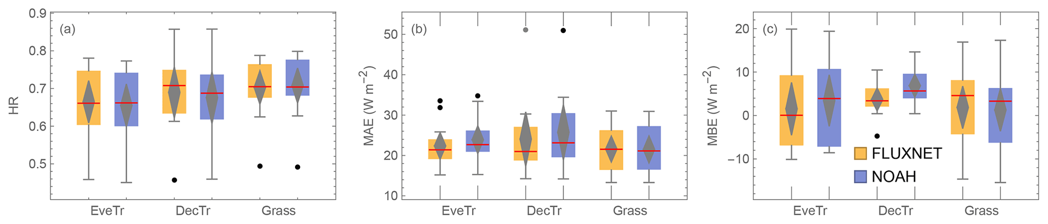
Figure 14 Simulated Q_E using two sets of parameters (colour, FLUXNET – Table C3, NOAH – Table A1 assigned based on Table 3 PFT class) at 38 sites (boxplots, as Fig. 9, subdivided into three land cover classes: EveTr, DecTr and Grass) evaluated for 2 years with observed 30 or 60 min fluxes using three metrics (Sect. 5.1): (a) HR, (b) MAE and (c) MBE.

Analysis using 2 years of Q_E EC flux data (after a 1-year spin-up) uses three metrics (Sect. 5.1). The overall median results are similar between the two sets of parameters across the 38 sites split into the three PFTs (Fig. 14, red lines). The median HRs are between 0.6 and 0.7, median MAEs are less than 25 W m⁻², and median MBEs are ∼ 5 W m⁻². At the Grass site, HR and MAE (Fig. 14a and b) performance is very similar, suggesting the NOAH-based parameters could be used for these sites at annual scales as a first-order proxy.

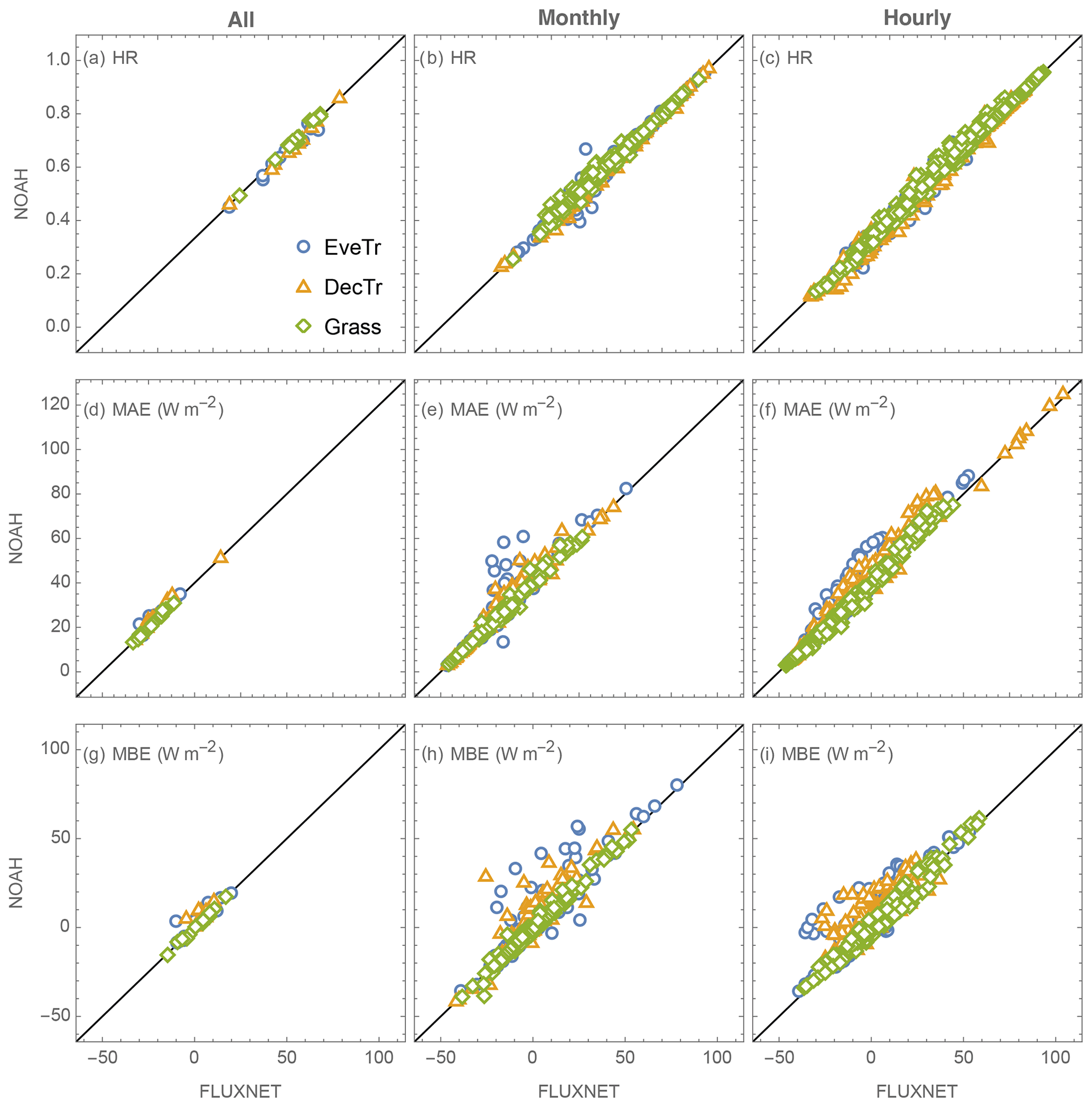
Figure 15 Relation between NOAH and FLUXNET of (rows) three evaluation metrics for (columns) three temporal scales (all, n=38 sites but different number of samples per site, Table 3; monthly, n = 456 = 38 sites × 12 months; and hourly, n = 912 = 38 sites × 24 h). Data points are colour coded by land cover class.

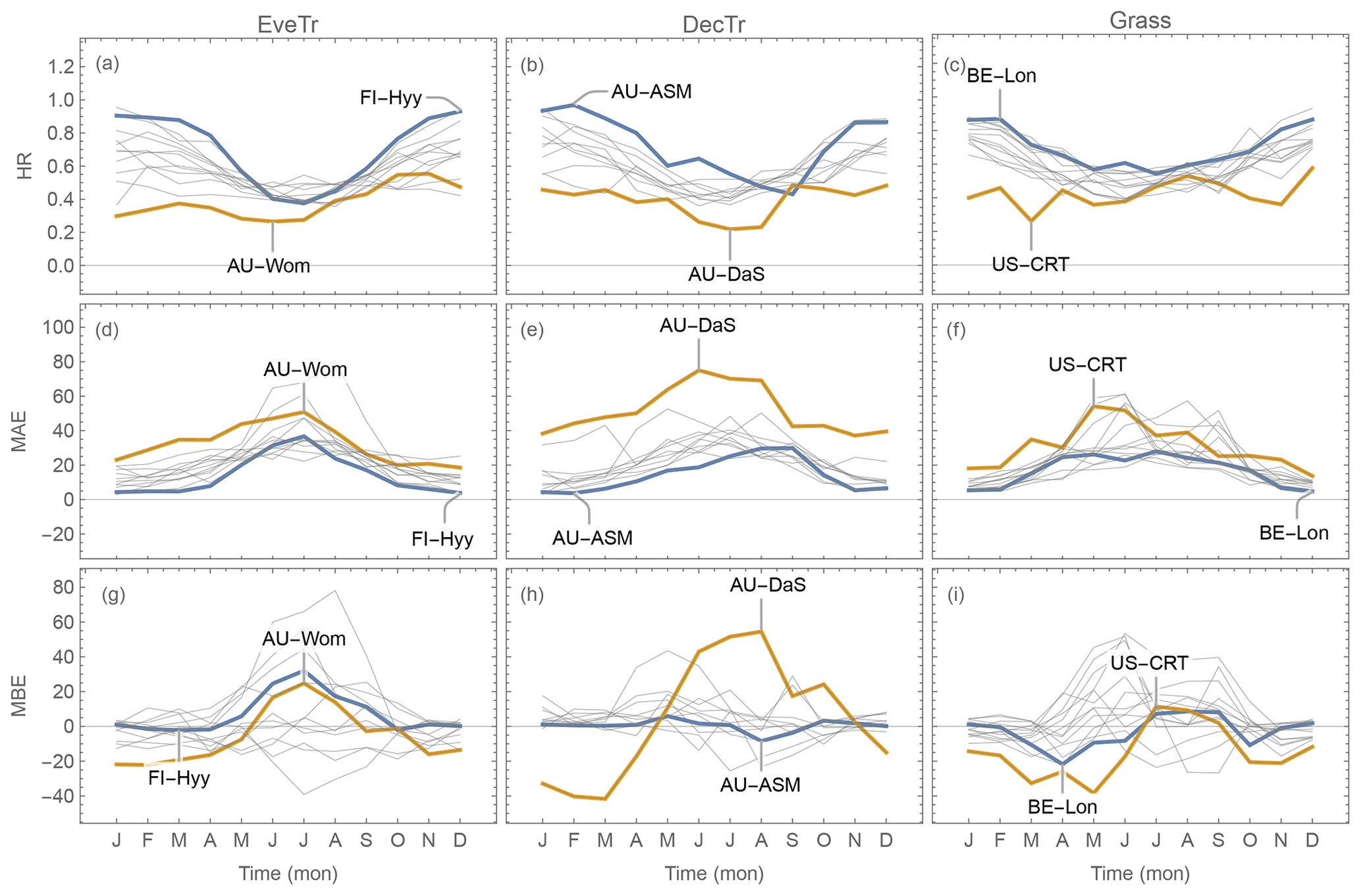
Figure 16 Variation in evaluation metrics (Sect. 5.2) based on 30 or 60 min Q_E data by month using the derived parameters based on FLUXNET2015 dataset (Tables C1–C3): (a–c) HR, (d–f) MAE, (g–i) MBE by sites grouped into three PFTs, (a, d and g) EveTr, (b, e and h) DecTr and (c, f and i) Grass with sites of best (blue) and poorest (orange) performance highlighted and others in grey (indicated by PS: see text and Eq. 35 for details). Note Southern Hemisphere sites are offset by 6 months (Sect. 5.1), so “general” seasons are consistent across sites.

Evaluation using three different time periods (annual, monthly and hourly) shows differences in performance between using the FLUXNET2015 and NOAH-based parameters (Fig. 15). The HR is similar for all three temporal scales (Fig. 15a–c) for the three site types (colour). Both the MAE (Fig. 15d–f) and MBE (Fig. 15g–i) indicate better model performance can be obtained using the FLUXNET2015-based parameters (i.e. not above the 1:1 line). When using the NOAH parameters (Fig. 15h and i), some monthly MBEs are ∼ 40 W m⁻² larger at EveTr sites for 8 of 156 cases and 5 of 312 for DecTr sites. Similarly, at the hourly scale the NOAH MBEs are on occasions ∼ 30 W m⁻² larger (4 of 132 EveTr cases and 6 of 264 DecTr cases). However, the NOAH results have similar metrics at Grass sites. This suggests at the EveTr and DecTr sites, the NOAH-based g_s parameters may on occasion be less appropriate, suggesting that the individual sites' values may be better.

Figure 17 As Fig. 16, but for diurnal cycles using local standard time.

5.4 Evaluation of SUEWS-simulated Q_E and key parameters at sites with contrasting model performance

Given the results in Sect. 5.3, the performance of individual sites using the FLUXNET2015-derived parameters (Sect. 4) at monthly (Fig. 16) and hourly (Fig. 17) timescales are investigated.

As expected (Sect. 5.2), the HR values are consistently better at all sites during cooler (winter) than warmer (summer) seasons (Fig. 16a–c), and similarly for night rather midday time periods (Fig. 17a–c). Given the consistency in MAE and HR (Figs. 16 and 17d–f) patterns, the sites identified to be simulated the “best” (blue) and “poorest” (orange) are the same (Sect. 5.1).

However, using the MBE different sites are selected. For example, monthly MBE at AU-ASM stays close to zero throughout the year while at AU-Das it varies between −40 and 60 W m⁻² (Fig. 16h). The largest intra-month MBE range for an EveTr site is 87.1 W m⁻², which occurs at FR-LBr. The equivalent range for DecTr sites is larger (96.1 W m⁻² at AU-DaS) but smaller at Grass sites (69.6 W m⁻²; US-Ne3). The intra-hourly MBE ranges are smaller than intra-monthly values, with a DecTr and a Grass site having a larger range than the largest EveTr site (AU-DaS (61.9 W m⁻²), US-Goo (60.0 W m⁻²), FR-LBr (53.1 W m⁻²), respectively).

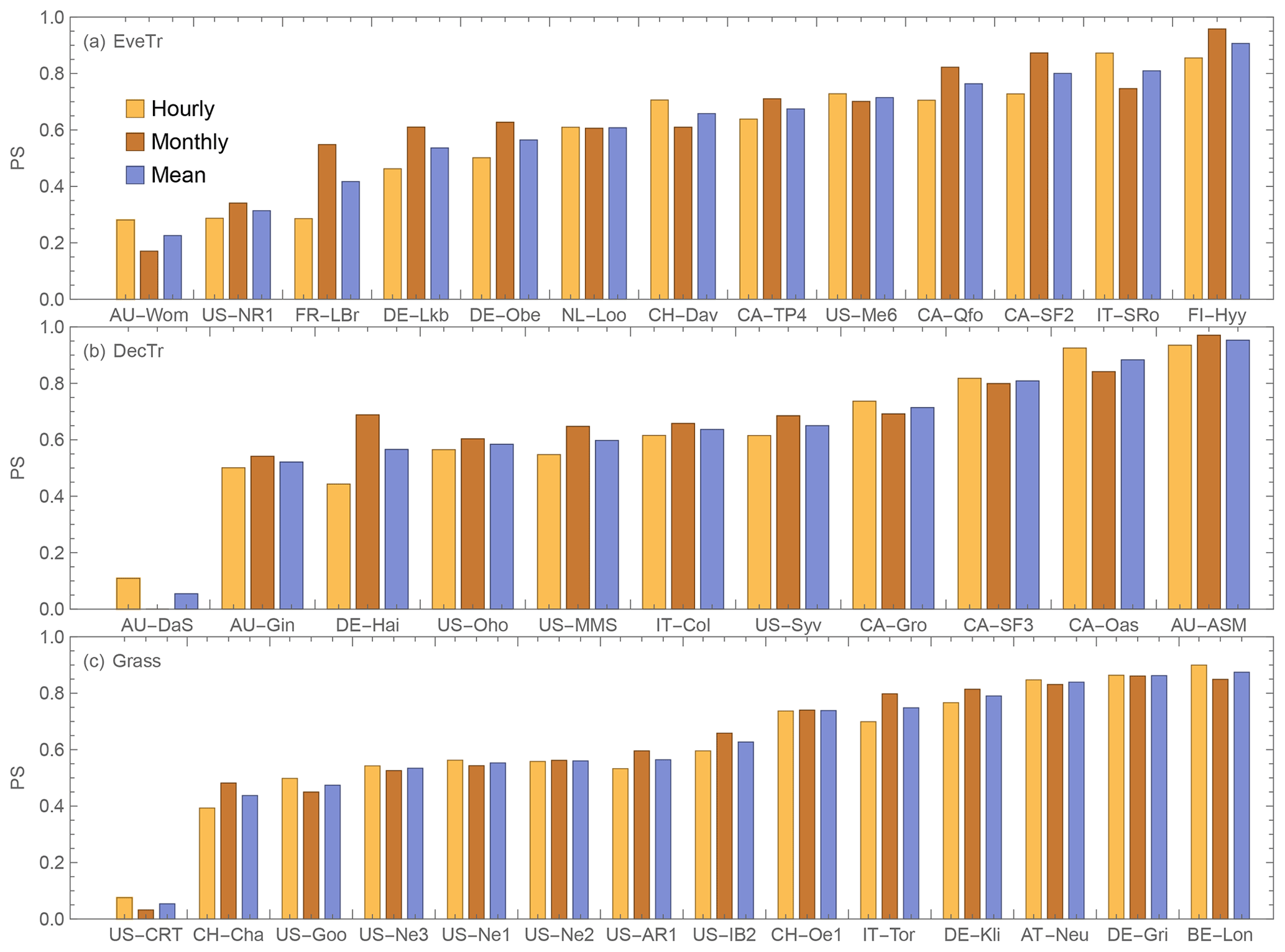
Figure 18 Performance score (PS, Eq. 35, higher value better) using FLUXNET2015 derived parameters for sites (Table 3) from three PFT: (a) EveTr, (b) DecTr and (c) Grass.

To investigate Q_E performance relative to key parameters (LAI, r_a and g_s) we select the sites with contrasting results from each PFT to understand the drivers. The hourly and monthly ranked performances (Eq. 35) are broadly consistent within each PFT (Fig. 18). Sites with higher hourly scores generally have better monthly scores, except for IT-SRo within the EveTr cohort. It has the highest hourly PS (0.86) but is ranked fourth based on PS_monthly (0.64), whereas the highest PS_monthly (0.91) is for FI-Hyy which also has the second rank PS_hourly (0.83). To select sites for further analysis we rank based on the mean of monthly and hourly PS results. The six sites chosen are the best and poorest sites for the three PFTs (i.e. extremes in Fig. 18, highlighted in Figs. 16 and 17).

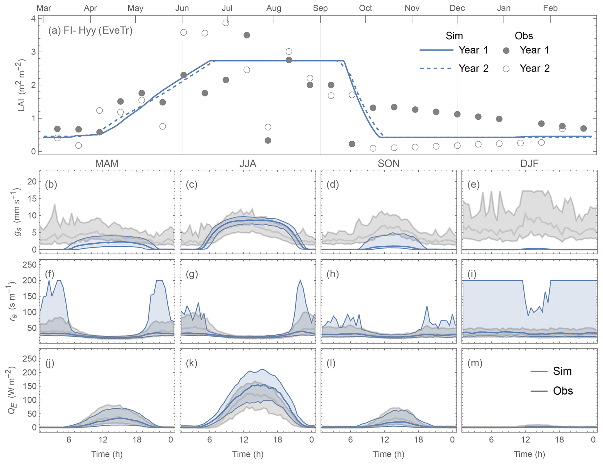
Figure 19 FI-Hyy (EveTr, PS = 0.92) performance: (a) annual LAI, (b–e) g_s (in seasonal ensemble of diurnal cycles: median values in bold lines, while interquartile ranges in shadings), (f–i) r_a and (j–m) Q_E. Note the same colouring of simulations for sites with best and poorest model performance and 6-month offset in annual cycles are applied for consistency with Figs. 16 and 17.

Figure 20 As Fig. 19, but for AU-Wom (EveTr, PS = 0.18).

Figure 21 As Fig. 19, but for AU-ASM (DecTr, PS = 0.96).

Figure 22 As Fig. 19, but for AU-DaS (DecTr, PS = 0.04).

Figure 23 As Fig. 19, but for BE-Lon (Grass, PS = 0.88).

Figure 24 As Fig. 19, but for US-CRT (Grass, PS = 0.04).

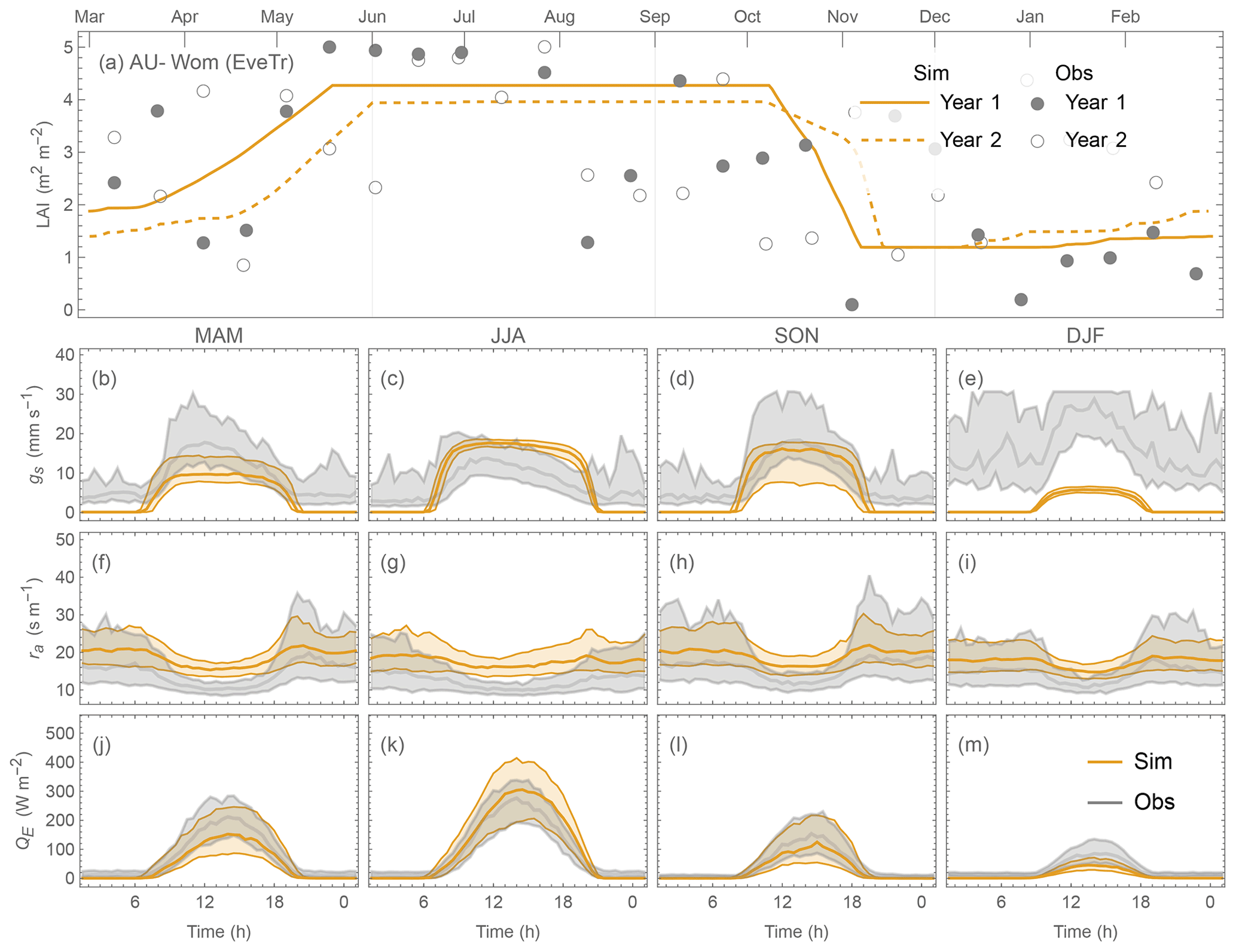
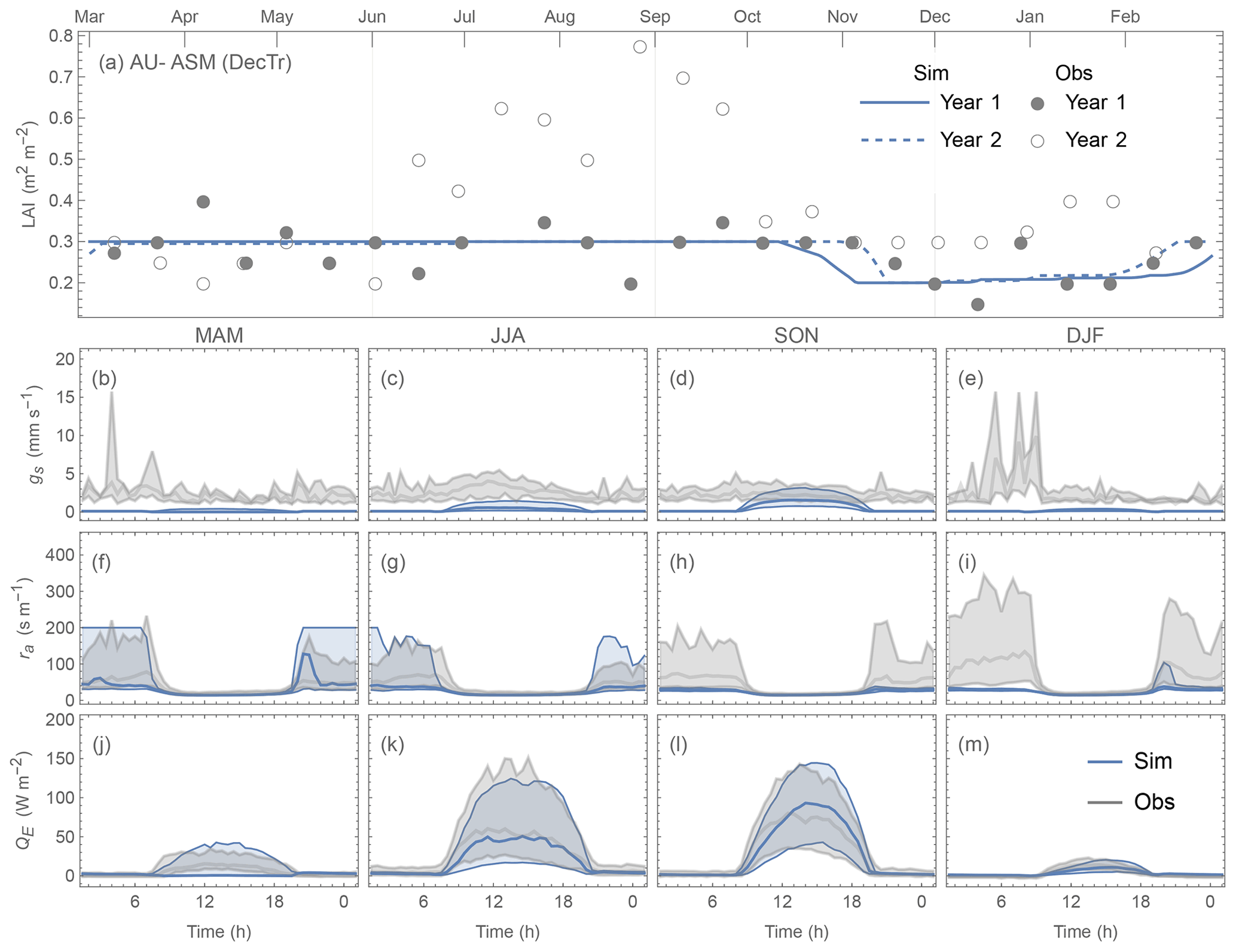
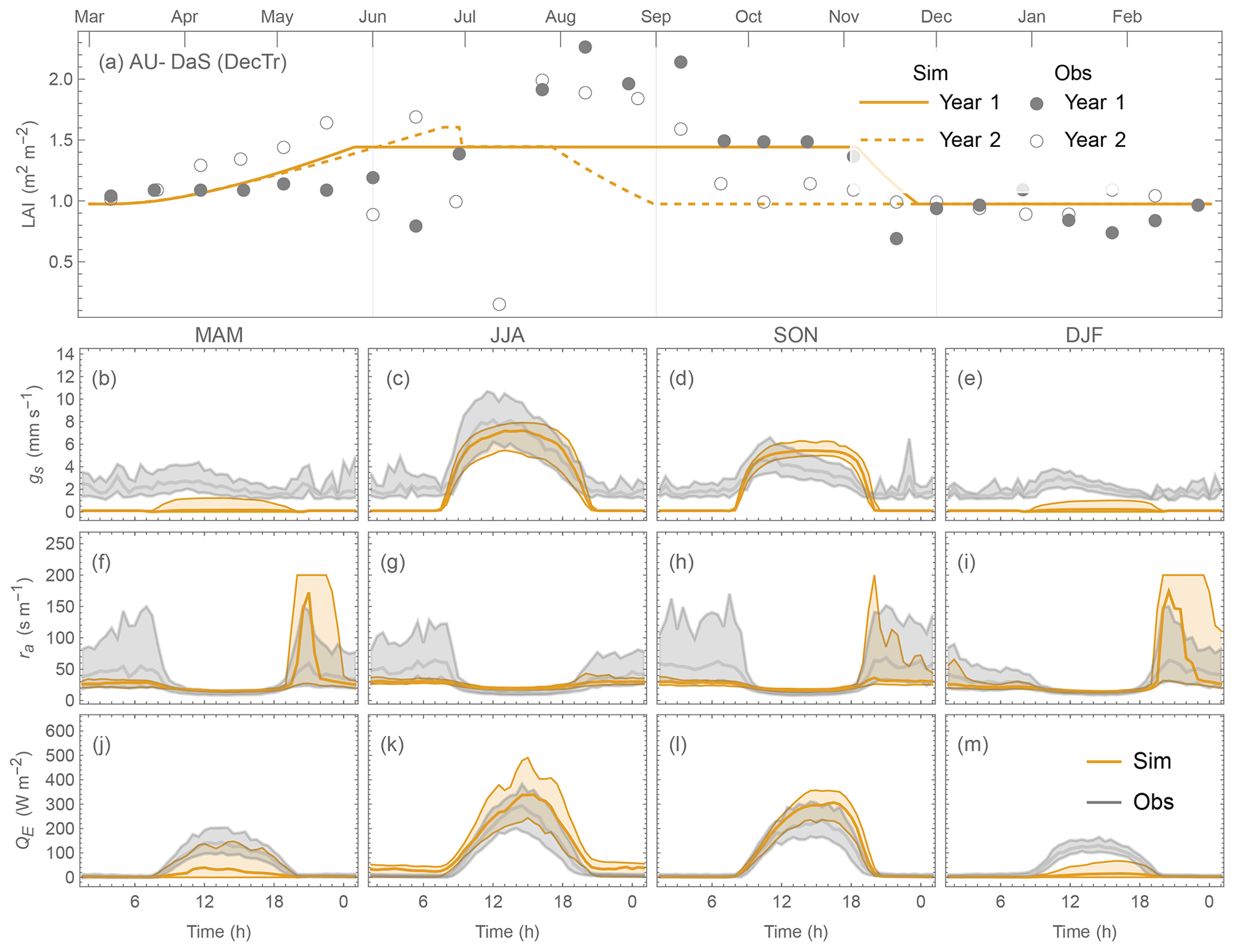
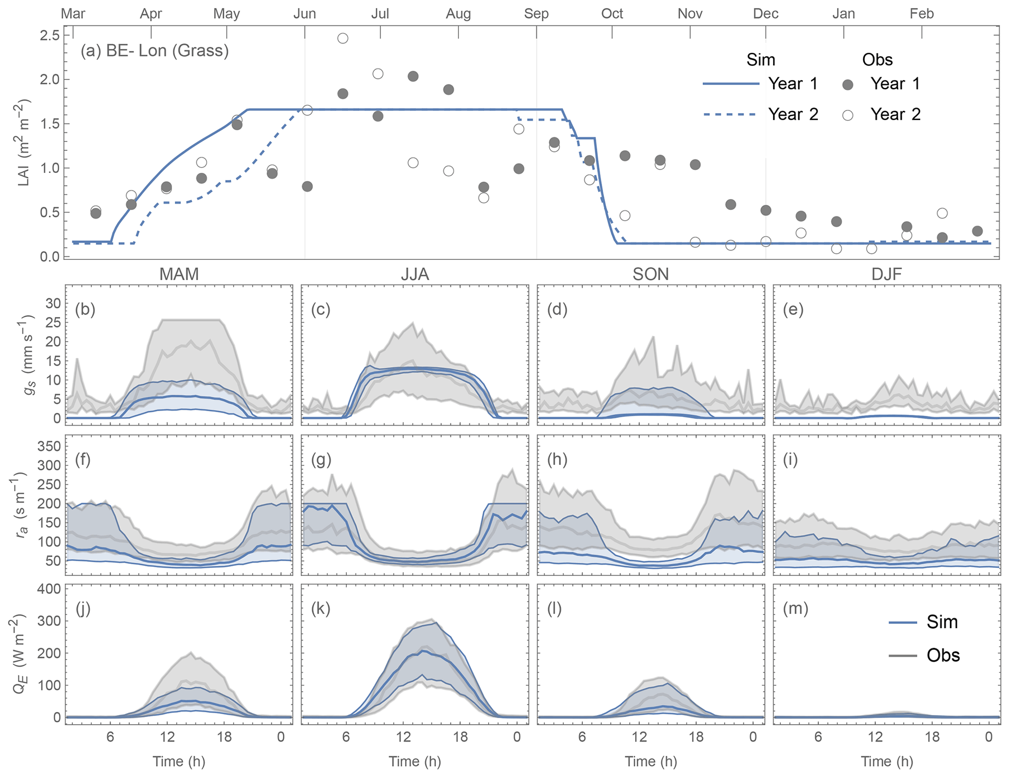
Comparing the contrasting site Q_E performance (best vs. poorest) for the three PFTs (Figs. 19 vs. 20; 21 vs. 22; 23 vs. 24), we identify the skill of capturing the annual LAI dynamics is crucial to seasonal model performance (Figs. 19–24a). At the “best” sites (except for BE-Lona, a Grass site whose performance is more controlled by surface conductance g_s skill and shall be discussed later) the phenology generally has the correct timing, while at the poorest onsets of some stages are missed (e.g. Fig. 22a). Timing appears to be more critical than magnitude, as although the LAI magnitude at AU-ASM has a large bias in year 2 (0.5 m² m⁻², Fig. 21a) the phenology timing is well captured. This result for a first rank site (i.e. best performance) implies the rescaling nature of LAI in parameterisation of albedo (Eq. 6) and surface conductance (Eq. 14) plays an important role. This indicates the importance of assigning appropriate LAI parameters, notably those influencing the timing (i.e. temperature thresholds T_base,GDD and T_base,SDD in Eq. 4), in SUEWS modelling Q_E at vegetated sites.

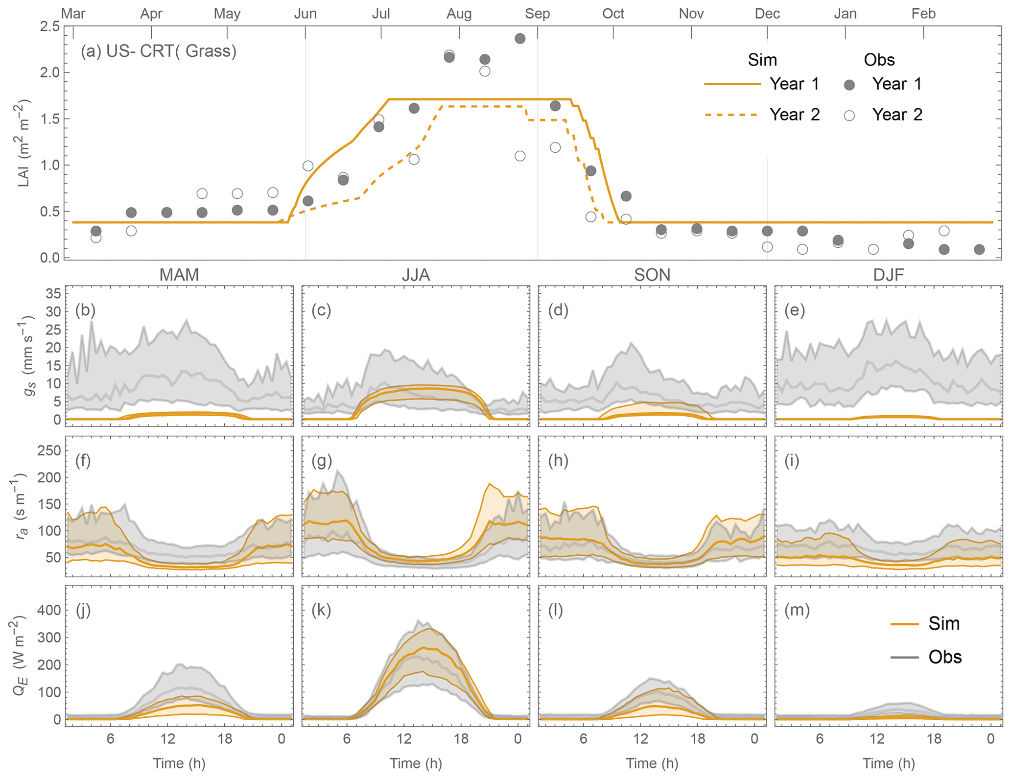
As expected (Sect 5.2), SUEWS performance is critically impacted by surface conductance g_s skill (Figs. 19–24b–e vs. j–m): sites and seasons with better model g_s skill (i.e. simulations and observations closer) show overall better performance (e.g. for Grass sites, BE-Lon vs. US-CRT, cf. Figs. 23c and 24c). g_s is better modelled in warmer (JJA and SON) than cooler seasons (MAM and DJF). At night, g_s is generally underestimated, by a similar order of magnitude to that in cooler seasons (∼ 3 mm s⁻¹). These results, consistent with SUEWS results for two UK urban sites (Ward et al., 2016), suggest improvements are needed in the Jarvis-type g_s parameterisation during cooler periods. Given the method adopted here of using summertime observations, as used by many other land surface models (e.g. NOAH – Chen and Dudhia, 2001; HTESSEL – Balsamo et al., 2009), it is implied that the widely adopted Jarvis-type g_s parameterisations and/or related parameter values (see Sect. 4.3) may be biased towards vegetation canopies in warmer periods. The “cool” bias in modelled g_s found here, and in earlier SUEWS work (e.g. Ward et al., 2016), should be considered a more common issue beyond the SUEWS model. Given the needs in long-term climate modelling, systematic biases should be removed, suggesting other land surface models that adopt the Jarvis-type g_s parameterisation might need revisions as well.

The aerodynamic resistance r_a is modelled well at all sites (Figs. 19–24f–i), with nocturnal biases larger (e.g. underestimate of ∼ 50 s m⁻¹ at AT-Neu, Fig. 23f–i). This good performance may be largely attributed to the use of local growth-stage-derived aerodynamic roughness parameters (Appendix B) rather than estimated using a morphometric model (e.g. based on canopy height). To estimate z_0m and z_d using Eqs. (9) and (10) the f₀ and f_d parameters can be derived using Sun et al. (2021) for different growing stages with the FLUXNET2015 data when canopy heights are available. The largest intra-PFT variability occurs for “Grass” sites (Fig. B1).

6 Concluding remarks

In this work, we derive parameters for SUEWS for fully vegetated land covers that are commonly found in background (“rural”) contexts of cities, where SUEWS has been widely used to model urban climates. To facilitate derivation of SUEWS parameters we provide workflows in Jupyter notebooks (Sun et al., 2021) for leaf area index (LAI), albedo, Objective Hysteresis Model (OHM) coefficients, aerodynamic roughness parameters and surface conductance (g_s). We use these to determine parameters at 38 vegetated FLUXNET sites in North America, Europe and Australia. Using the derived parameters, we assess the performance of SUEWS in predicting latent heat flux (Q_E) at different temporal scales (monthly and hourly).

The following conclusions were made:

• Where observations are available, we recommend determining local parameters, as derived parameters vary within PFT (Appendix C). The tools provided here are designed to facilitate this (Sect. 4).

• Given the global availability of MODIS LAI and reanalysis-based air temperature datasets (e.g. ERA5), it is feasible to derive site-by-site LAI parameters for SUEWS (Sect. 4.1).

• OHM coefficients for modelling storage heat flux derived here show clear seasonality: summertime (i.e. days warmer than annual median air temperature) a₁ and a₃ are smaller than their wintertime counterparts, while the seasonal contrast in a₂ is smaller, suggesting seasonally varying values should be used for long-term (i.e. > 1 year) simulations.

• Surface-conductance-related parameters derived using a summertime upper-boundary-based approach (Matsumoto et al., 2008) produce parameters related to solar radiation (G_K) and optimal air temperature (G_T) with some dependence on geographical locations, which could be used as a proxy to derive these two parameters.

• SUEWS-modelled Q_E is particularly sensitive to surface conductance as informed by the attribution analysis using an analytical framework by McCuen (1974) and consistent with results of Beven (1979) that surface conductance plays a dominant role in moderating the bias in modelled Q_E.

• SUEWS configured with NOAH-based parameters has comparable prediction skill in Q_E compared to site-specific parameters when assessed by hit rate (HR) with medians being ∼ 0.65. However, site-specific parameters improve SUEWS performance as shown by the mean absolute error (MAE) and mean bias error (MBE) metrics, becoming increasingly evident at finer temporal scales (monthly and hourly).

• SUEWS with site-specific parameters outperforms in cooler periods (i.e. winter and night) compared to warmer periods (i.e. summer and day): HR is consistently higher in the former periods than the latter (0.71 vs. 0.52 in median) while MAE shows an opposite pattern (cooler vs. warmer seasons median: ∼ 12 vs. ∼ 31 W m⁻²).

• Correctly predicting LAI timing dynamics has a crucial influence on overall Q_E model performance, followed by surface conductance g_s that is generally underestimated during cooler periods (more pronounced at night by ∼ 3 mm s⁻¹).

As the first comprehensive study of SUEWS at multiple vegetated sites, we also identify future development and application needs:

• None of the simple LAI schemes in SUEWS account for hydrological impacts on LAI. Vegetation with shallow roots (e.g. US-SRG in Arizona, US, categorised as GRA according to IGBP, Fig. D2) are not well modelled when air temperature is the only phenology forcing variable. Hydrological feedback should be considered in future development of the LAI scheme in SUEWS.

• The specific humidity deficit surface conductance parameter relation needs improvement as a plateau-like trend is observed near the lower end (e.g. Fig. 9c).

• A potential source of parameter values for PFT beyond those studied here (i.e. values provided Appendix C, Sun et al., 2021) could be NOAH-based parameters (Appendix A) but these should be used with caution, as demonstrated (Sect. 5).

• More careful treatment of snow cover should be incorporated to enhance SUEWS capacity in high-latitude regions.

Appendix A: NOAH-based equivalent values for surface-conductance-related parameters for SUEWS

The NOAH land surface scheme (Chen et al., 1996) uses a similar Jarvis-type parameterisation of surface conductance g_s to that in SUEWS (i.e. Eq. 13) but with different formulation of g_s sub-components from SUEWS (Eqs. A1–A4 vs. Eqs. 15–18). The NOAH equations using our notation are as follows:

• Incoming solar radiation (K_↓).

  $$\begin{array}{}\text{(A1)}& g_{\text{NOAH}}\left(K_{\downarrow }\right)={\displaystyle \frac{\frac{R_{\text{cmin}}}{\mathrm{5000}}+f}{\mathrm{1}+f}},\end{array}$$

  where $f=\mathrm{0.55}\frac{K_{\downarrow }}{R_{\mathrm{g}l}}\frac{\mathrm{2}}{\text{LAI}}$ with R_gl an adjustable parameter for K_↓.

• Air specific humidity (q).

  $$\begin{array}{}\text{(A2)}& g_{\text{NOAH}}\left(q\right)={\displaystyle \frac{\mathrm{1}}{\mathrm{1}+h_{\mathrm{s}}(q_{\mathrm{s}}-q)}},\end{array}$$

  where h_s is the adjustable parameter for specific humidity q and q_s the saturation specific humidity.

• Air temperature (T_a).

  $$\begin{array}{}\text{(A3)}& g_{\text{NOAH}}\left(T_{\mathrm{a}}\right)=\mathrm{1}-\mathrm{0.0016}(T_{\text{ref}}-T_{\mathrm{a}}{)}^{\mathrm{2}},\end{array}$$

  where T_ref is the adjustable parameter for air temperature T_a.

• Soil moisture (θ_soil).

  $$\begin{array}{}\text{(A4)}& g_{\text{NOAH}}\left({\mathit{\theta }}_{\text{soil}}\right)={\displaystyle \frac{{\mathit{\theta }}_{\text{soil}}-{\mathit{\theta }}_{\text{WP}}}{{\mathit{\theta }}_{\text{FC}}-{\mathit{\theta }}_{\text{WP}}}},\end{array}$$

  where θ_FC and θ_WP are field capacity and wilting point (see Table A2 for values of different soil types).

To use the NOAH parameters (as given in Tables 1 and 2 of Chen and Duhdia, 2001), we convert the NOAH parameters (Eqs. A1–A4) to the SUEWS required parameters (i.e. for Eqs. 15–18). The resulting SUEWS parameters (Table A1) are used (Sect. 5) to produce results in Figs. 14 and 15 denoted by NOAH.

Except for the g_s function for air temperature – SUEWS and NOAH adopt the effectively same formulation – other g_s functions may produce different results even using the converted parameter values (Table A1). In particular, for the shortwave radiation and specific humidity (Fig. A1), the SUEWS values (blue) are higher than NOAH values (red) for all PFTs. The role of soil type (Table A2) on the soil moisture deficit function (Fig. A2) results in larger differences at dry and mid-wet extremes.

Table A1 NOAH-derived (data: based on Tables 1 and 2 of Chen and Duhdia, 2001) surface-conductance-related parameters for SUEWS.

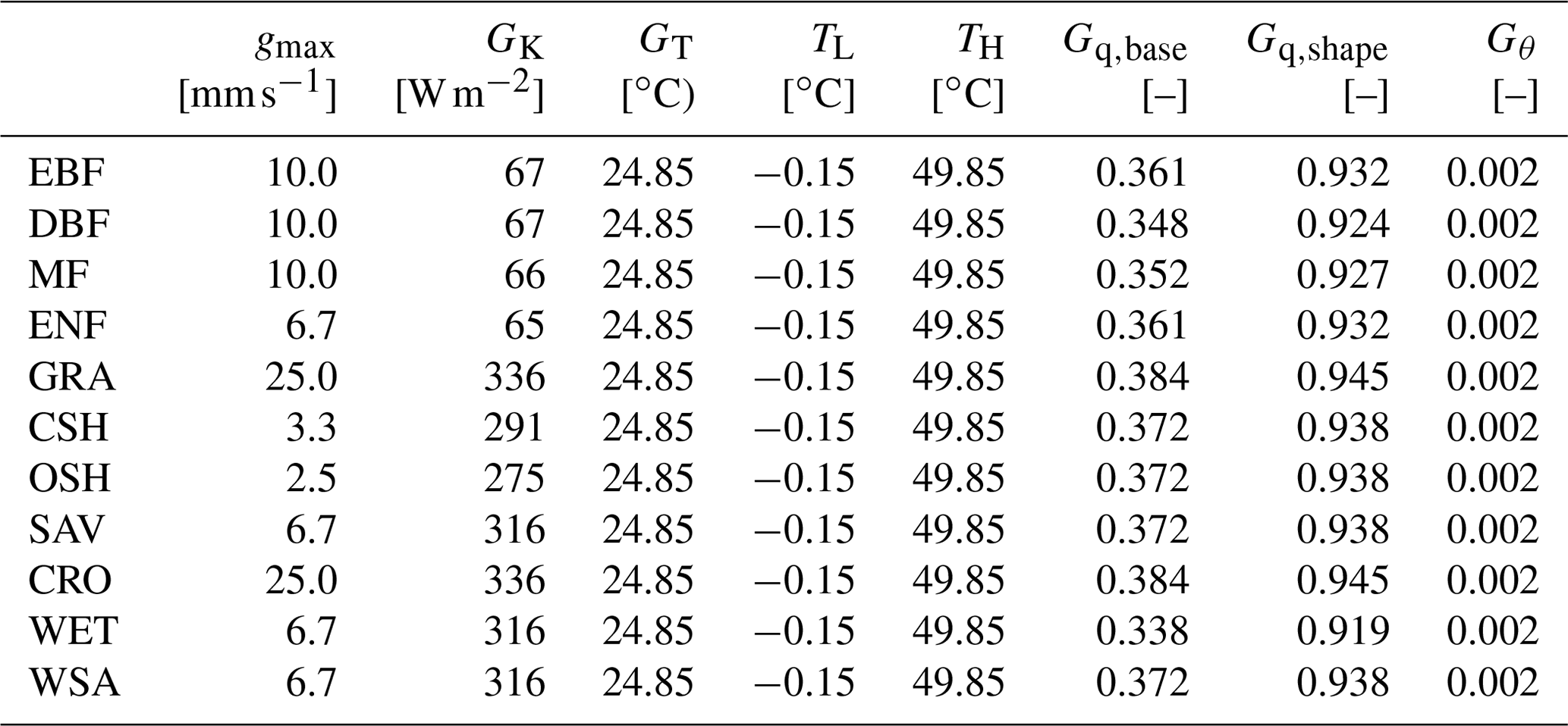
Table A2 Soil field capacity (θ_FC) and wilting point (θ_WP) used in NOAH (data: based on Table 2 of Chen and Duhdia, 2001).

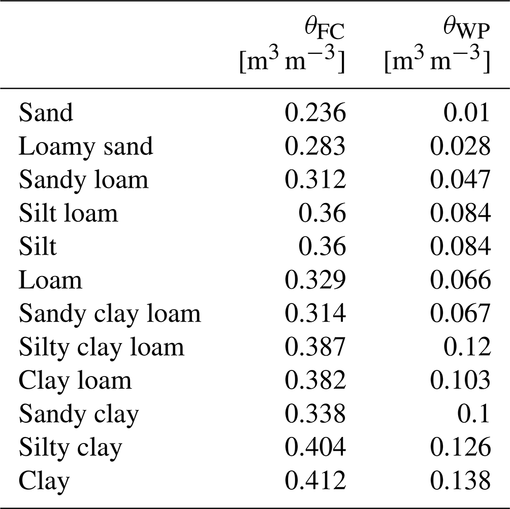
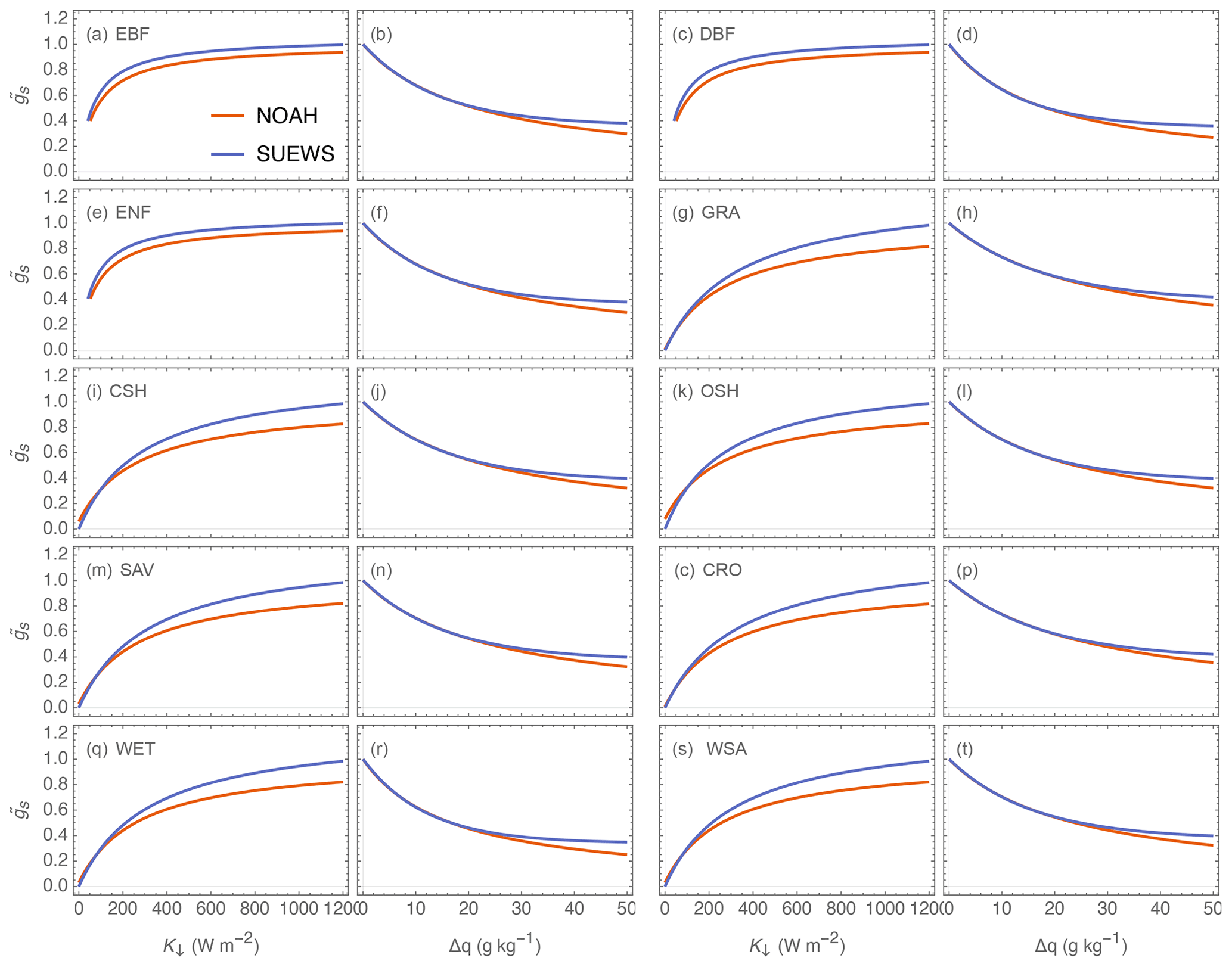
Figure A1 NOAH (red) and SUEWS (blue) surface conductance functions for incoming solar radiation (K_↓) and specific humidity deficit (Δq) for different IGBP PFTs.

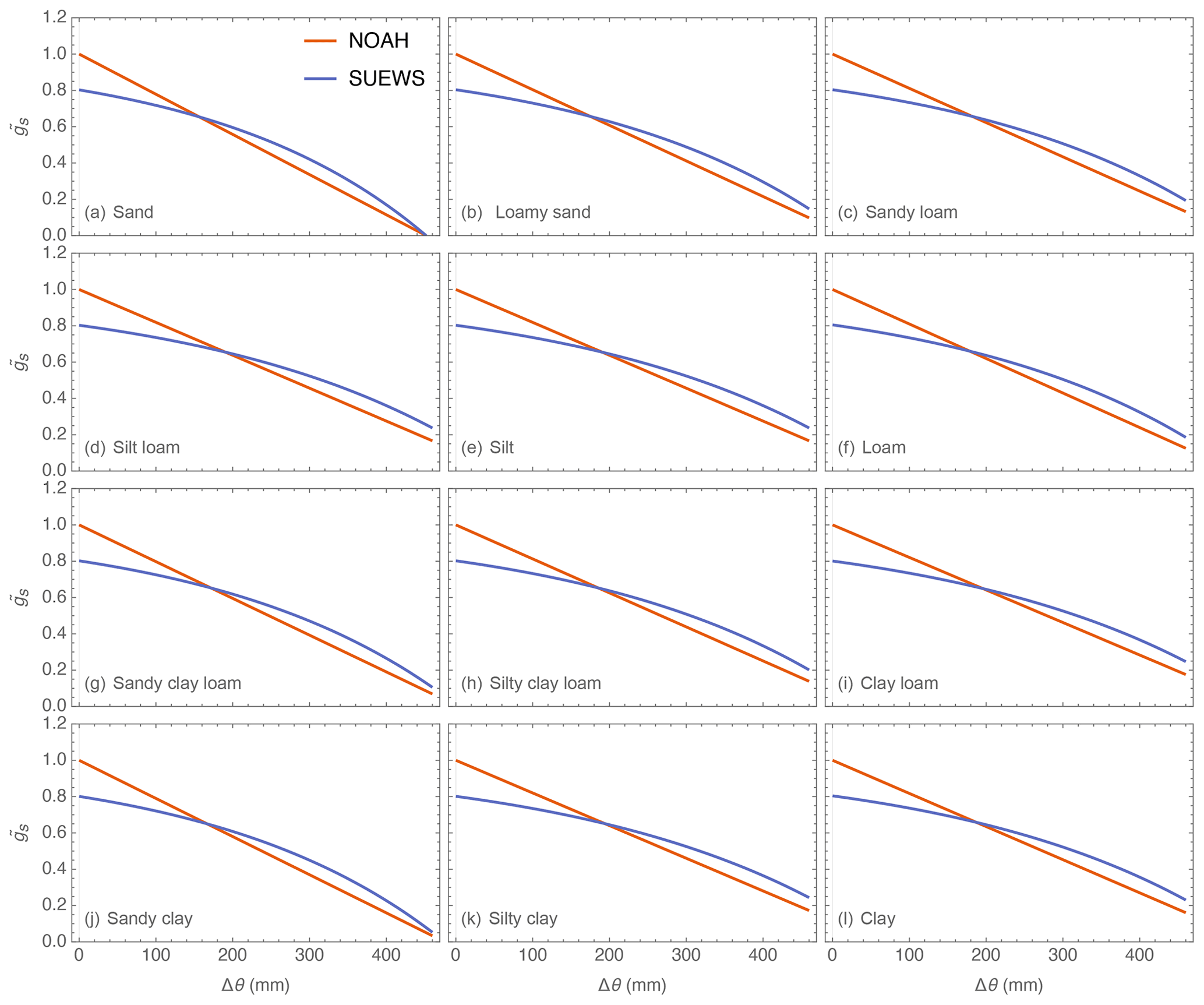
Figure A2 As Fig. A1 but for soil moisture deficit (Δθ) for different soil types with an assumed soil depth of 2000 mm. Soil hydraulic properties (field capacity θ_FC and wilting point θ_WP) are provided in Table A2.

Appendix B: Derivation of roughness length and zero-plane displacement height for momentum

The aerodynamic roughness parameters for momentum (roughness length z_0m and zero-plane displacement height z_d) are derived using observed u_∗ and u under neutral conditions (i.e. $\mathrm{|}\frac{z_{\mathrm{m}}-z_{\mathrm{d}}}{L}\mathrm{|}<\mathrm{0.01}$ with an initial estimate of z_d=0.7H_c) of different vegetation stages based on LAI (see Sect. 4.1 for classification details) by the least-square method for the following relation (Monin and Obukhov, 1954):

$$\begin{array}{}\text{(B1)}& u={\displaystyle \frac{u_{\ast }}{\mathit{\kappa }}}\ln \left({\displaystyle \frac{z_{\mathrm{m}}-z_{\mathrm{d}}}{z_{\mathrm{0}\mathrm{m}}}}\right),\end{array}$$

where κ is the von Kármán constant (0.4 is used here). In particular, for sites with varying canopy height H_c, z_0m and z_d are derived for each of the periods when H_c stayed unchanged and more than 20 observational pairs of u_∗ and u are available.

Using the derived z_0m and z_d, f₀ and f_d parameters can be obtained (Eqs. 9 and 10). These is considerable intra-PFT variability of both f₀ and f_d (Fig. B1). There are also intra-site variations associated with varying H_c. Given the large variability in both f₀ and f_d, the rule-of-thumb approach would incur a large bias in estimated aerodynamic and surface resistances and subsequently the modelled Q_E. To reduce such a bias, in the evaluation of the other sub-models and parameter determinations in this paper, we use the derive z_0m and z_d determined for each vegetation stage and site.

Modelled wind speed under neutral conditions matches well with observations at 38 study sites with MAE < 0.3 m s⁻¹ and MBE close to zero (Fig. B2). Of the three SUEWS PFTs, “Grass” sites have the poorer performance. This is probably because this PFT includes crops which will change frequently because of crop rotations: cereal, potato, sugar beet at BE-Lon (Moureaux et al., 2006); winter barley, rapeseed, winter wheat, maize and spring barley at DE-Kli (Prescher et al., 2010); and maize and soybean at US-Ne2 and US-Ne3.

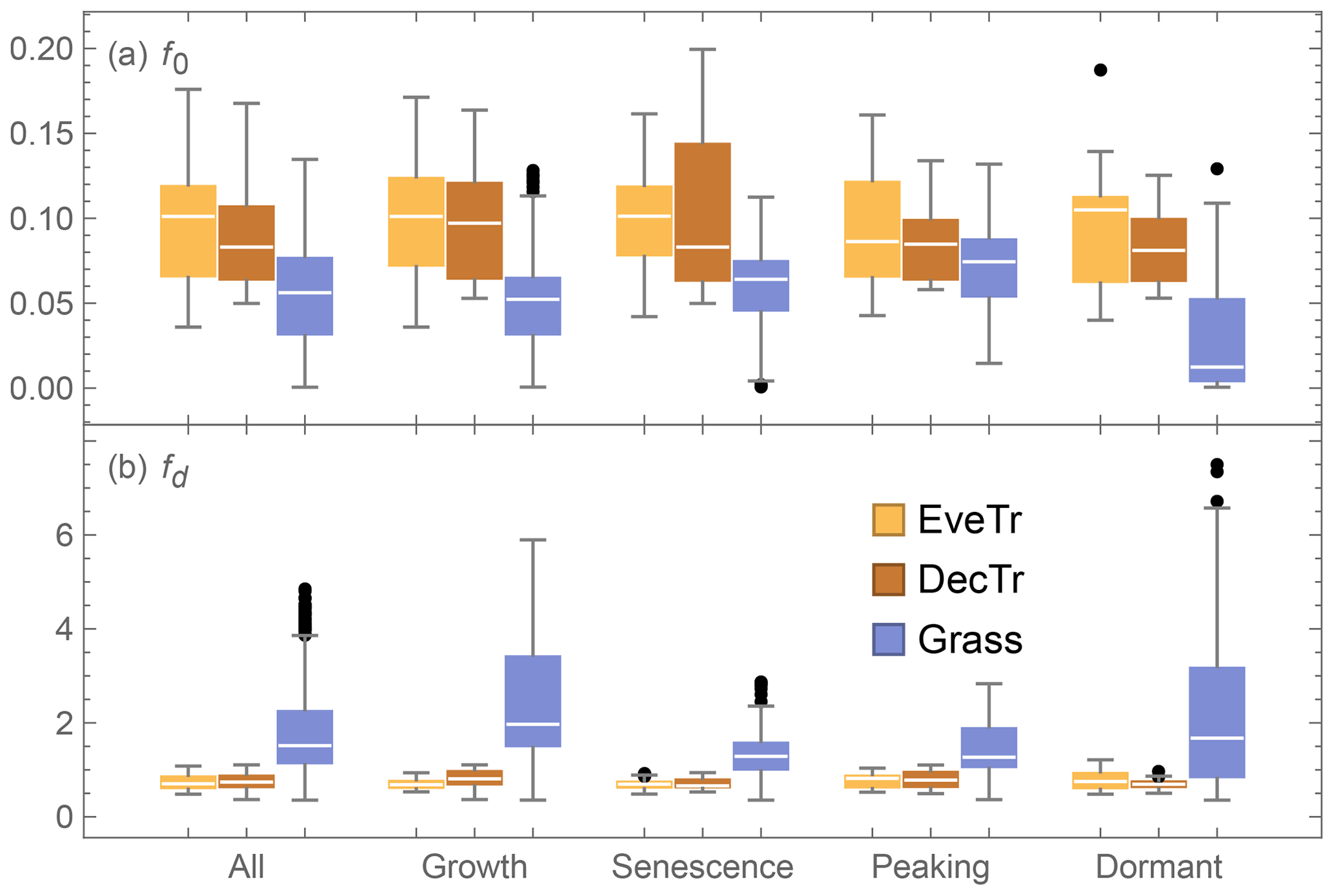
Figure B1 Relations between canopy height (H_c) and (a) roughness length for momentum (z_0m, Eq. B2) and (b) displacement height (z_d, Eq. B3) for different vegetation stages based on LAI (see Sect. 4.1 for classification details).

Figure B2 MAE (blue) and MBE (orange) for modelled wind speed under neutral conditions for three SUEWS PFTs: (a) EveTr, (b) DecTr and (c) Grass.

Appendix C: SUEWS parameters derived at selected FLUXNET sites

Table C1 LAI- and albedo-related parameters at 38 sites (Table 3 gives site information) derived using FLUXNET2015 dataset (Sect. 4.1).

Table C2 As Table C1 but for OHM-related parameters (Sect. 4.2).

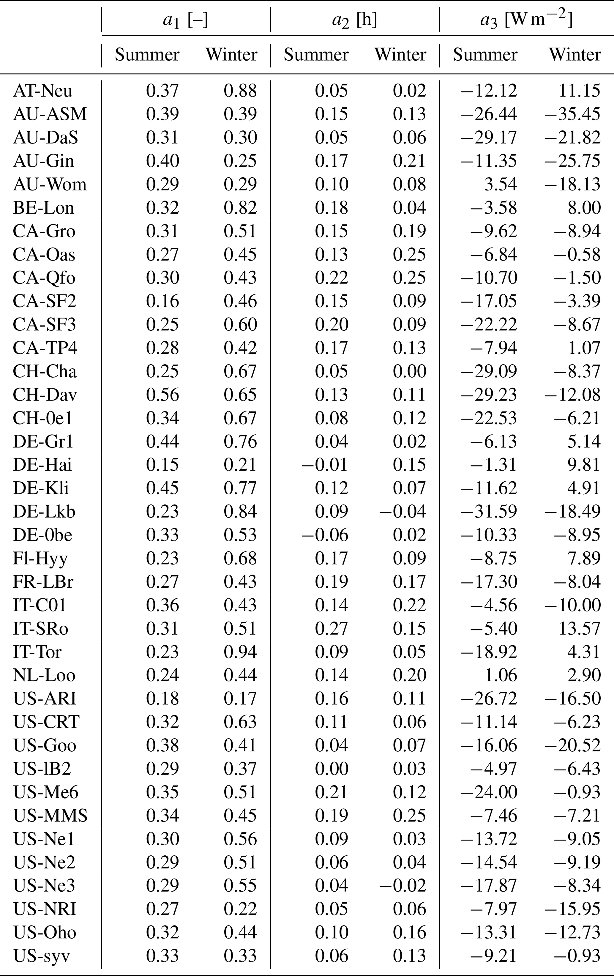
Table C3 As Table C1, but for surface-conductance-related parameters (Sect. 4.3).

Appendix D: Typical intra-annual LAI dynamics under contrasting meteorological controls

Given sufficient CO₂, vegetation phenology indicated by LAI dynamics is predominantly controlled by input energy and water (Fang et al., 2019). Two variables that capture this seasonal variability are air temperature and precipitation. Different intra-annual LAI dynamics are evident between sites, with contrasting meteorological controls:

• (a)

  Thermally dominant (US-MMS; Fig. D1). Intra-annual cumulative precipitation at US-MMS steadily increases throughout the year (Fig. D1a), implying a fairly even distribution of water supply, while air temperature gradually increases from the mid-winter (beginning of a year), peaks in August and decreases with the start of the next winter (Fig. D1b). The LAI pattern at US-MMS responds to the air temperature, notably the growing degree days (GDDs) and then autumn senescence (SDD). This inverse “U”-shape typifies sites with thermally dominant LAI dynamics. These types of sites are well parameterised by the current LAI scheme in SUEWS (Sect. 2.2.1).

• (b)

  Rainfall and thermal controls (US-SRG; Fig. D2). At this grassland site in Arizona, USA, the intra-annual precipitation has clear dry and wet seasons. The monsoon wet season after the peak air temperature in July through September (Fig. D2a), which has warmest air temperatures, unlike US-MMS (Fig. D2b), the peak air temperature is more distinct (for a shorter period). A clear relation between the onset of rainfall and LAI enhancement can be seen but the GDD and SDD relation differs from US-MMS, and it not captured by the current models in SUEWS. The rainfall and enhanced LAI and Q_E are associated with cooler daily air temperatures. Sites where the LAI dynamics are not captured are not explored further in this paper.

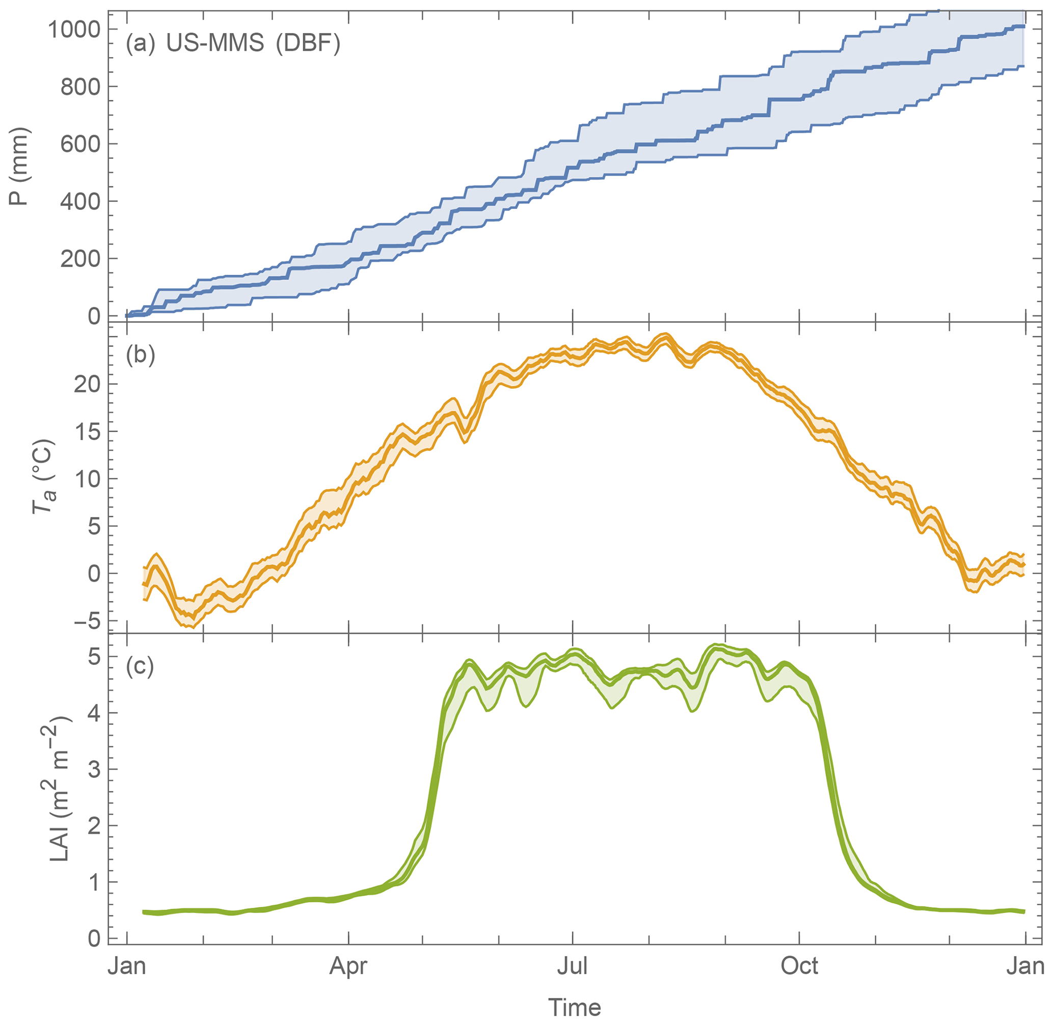
Figure D1 Median (line) and interquartile range (shading) daily variation at US-MMS a DBF site during the period 2002–2015 of (a) precipitation (cumulative), (b) air temperature (7 d moving average) and (c) LAI (7 d moving average).

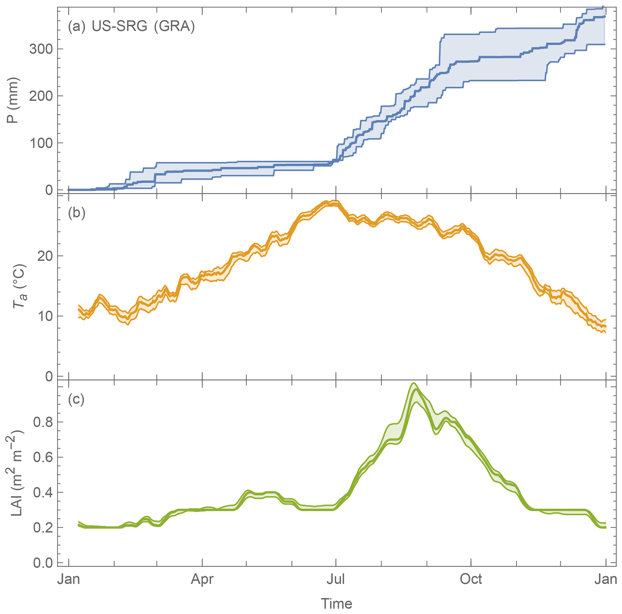
Figure D2 As Fig. D1, but for US-SRG (GRA according to IGBP; time span: 2008–2015; https://doi.org/10.18140/FLX/1440114).