Landslide Susceptibility Assessment Tools v1.0.0b – Project Manager Suite: a new modular toolkit for landslide susceptibility assessment

This paper introduces the Landslide Susceptibility Assessment Tools – Project Manager Suite (LSAT PM), an open-source, easy-to-use software written in Python. Primarily developed to conduct landslide susceptibility analysis (LSA), it is not limited to this issue and applies to any other research dealing with supervised spatial binary classification. LSAT PM provides efficient interactive data management supported by handy tools in a standardized project framework. The application utilizes open standard data formats, ensuring data transferability to all geographic information systems. LSAT PM has a modular structure that allows extending the existing toolkit by additional tools. The LSAT PM v1.0.0b implements heuristic and data-driven methods: analytical hierarchy process, weights of evidence, logistic regression, and artificial neural networks. The software was developed and tested over the years in different projects dealing with landslide susceptibility assessment. The emphasis on model uncertainties and statistical model evaluation makes the software a practical modeling tool to explore and evaluate different native and foreign LSA models. The software distribution package includes comprehensive documentation. A dataset for testing purposes of the software is available. LSAT PM is subject to continuous further development.

1 Introduction

Landslides occur in all mountainous parts of the world, significantly contributing to disastrous socioeconomic consequences and claiming thousands of casualties every year (Petley, 2012; Froude and Petley, 2018). These phenomena are frequently associated with other natural hazards such as severe rainfall, floods, and earthquakes (e.g., Polemio and Petrucci, 2000; Crozier, 2010; Keefer, 2002; Kamp et al., 2008).

Per definition, a comprehensive assessment of landslide hazards addresses the spatial and temporal landslide occurrence based on three questions: Where? When? How large? (e.g., Varnes, 1984; Guzzetti et al., 1999; Tanyaş et al., 2018; Reichenbach et al., 2018). Landslide susceptibility analysis (LSA) depicts the probability of spatial landslide occurrence (e.g., Brabb, 1985; Guzzetti et al., 2005) covering the spatial domain of the hazard analysis. Addressing the temporal domain of landslide hazard assessment is much more challenging due to the local character of the phenomenon and a common lack of multi-temporal landslide inventories covering sufficient periods (e.g., Aleotti and Chowdhury, 1999; Van Westen et al., 2006). Therefore, most case studies at regional scales focus on LSA as the most feasible part of the landslide hazard analysis.

Regional LSA is usually done based on qualitative (heuristic or knowledge-driven) and quantitative methods (Reichenbach et al., 2018). The quantitative techniques comprise physically based and data-driven statistical, as well as machine learning (ML) approaches (e.g., Aleotti and Chowdhury, 1999). The desired analysis scale and data availability usually govern the decision of which method to use (e.g., Van Westen et al., 2008; Balzer et al., 2020).

In the past decades, advances in remote sensing have made significant progress, allowing efficient data acquisition at regional scales. Additionally, digitalization forced a general boost of data mining techniques. Together with the development of Geographic information system (GIS) software packages and open-source statistical and machine learning libraries, the data-driven methods for LSA have gained popularity. These methods belong mainly to supervised binary classification (e.g., Torizin, 2016). In the supervised classification, we use a set of recorded observations (labels) and independent explanatory factors (features) such as different geomorphologic, hydrologic, and geological conditions to train a statistic function (classifier). The classifier estimates the likelihood of a specific countable element in a study area (e.g., raster pixel) to be in the specified target class (e.g., landslide or no landslide).

Because classification is one of the fundamental tasks in statistics and ML, many different classifiers exist. Consequently, in numerous case studies, the academic community continuously applies and compares classification algorithms and their variations, which were initially developed for other purposes but are sufficiently general to be used for LSA. While some classifiers might outperform others, the drawn conclusions are often valid only for particular settings and study designs (e.g., Balzer et al., 2020). Under other circumstances, such as different data quality or distribution, it is very likely that some of the other classifiers perform on par or better. Reviewing the LSA research of the past 30 years, Reichenbach et al. (2018) counted about 163 different data-driven methods, emphasizing the problem of excessive experimentation with statistical classifiers rather than focusing on LSA reliability. Many of these methods have never been adopted or seriously considered by practitioners skeptically following the academic research at their own pace and utilizing a comparably small part of it. Thus, despite the many academic publications dealing with regional data-driven LSA, only a few practical solutions have been adopted in national landslide risk assessment strategies (e.g., Balzer et al., 2020). Also, user-friendly stand-alone software developed in this field is rare compared to the available geotechnical software applications. Many available tools exist as academic code generated to support specific case studies (e.g., Merghadi, 2018, 2019; Egan, 2021; Raffa, 2021) and imply that the user has the necessary programming or scripting skills to set up and run the tools. Despite considerable efforts to adapt the Earth science curricula to digital transformation (e.g., Hall-Wallace, 1999; Makkawi et al., 2003; Senger et al., 2021), the required computational literacy to deal with those applications is not a broad standard in geosciences. However, there is a positive trend. Rising education possibilities on e-learning platforms with exhaustive offers in programming narrow the gap between geosciences and data sciences. Bouziat et al. (2020) noted that the geoscience community increasingly uses Python (Van Rossum and Drake, 2009) for data processing, the R statistical package (R Core Team, 2013) for statistical analysis, and custom web services for sharing results.

Since 2010, many LSA tools have been available as plugins or extensions in different GIS such as LSAT (Polat, 2021), LSM Tool Pack (Sahin et al., 2020), or ArcMAP Tool (Jebur et al., 2015) in ESRI ArcGIS, SZ-plugin (Titti et al., 2021) in QGIS (QGIS Development Team, 2022), r.landslide (Bragagnolo et al., 2020a) in GRASS GIS (GRASS Development Team, 2021), and RSAGA (Brenning, 2008) in SAGA, as well as scripts in R statistical packages, e.g., LAND-SE (Rossi and Reichenbach, 2016), and a few stand-alone applications, e.g., GeoFIS (Osna et al., 2014).

With the Landslide Susceptibility Assessment Tools – Project Manager Suite (LSAT PM), we introduce an open-source (GNU General Public License v3), stand-alone, and easy-to-use tool that supports scientific principles of openness, knowledge integrity, and replicability. Doing so, we want to share our experience in implementing heuristic and data-driven LSA methods. Our primary goal is not to introduce as many algorithms as possible for LSA but to provide easy access to a selection of state-of-the-art methods representing groups of different approaches. Providing a convenient framework for model building, evaluation, and uncertainty assessment, we want to highlight the capabilities and limitations of those methods.

2 LSAT PM software

LSAT PM is a desktop application designed to support decision-makers and the scientific community in generating and evaluating landslide susceptibility models based on heuristic and data-driven approaches.

2.1 Development history

The development of Landslide Susceptibility Assessment Tools (LSAT) started in 2011 with Python scripting within ESRI ArcGIS 10.0 Toolbox to support technical cooperation (TC) projects (Torizin, 2012). TC projects are usually not cutting-edge research but summarize, adapt, and implement scientific outcomes by following the best-practice approach. Since then, LSAT was continuously improved and tested at different development stages in case studies in Indonesia (Torizin et al., 2013), Thailand (Teerarungsigul et al., 2015), Pakistan (Torizin et al., 2017), China (Torizin et al., 2018), and Germany (Balzer et al., 2020). Working with different data of varying quality helped us develop efficient methodical workflows. It also enabled us to better understand the limitations of some methods and design practical approaches to assess model uncertainties (e.g., Torizin et al., 2021).

In 2017, we started to prototype LSAT as a stand-alone application bearing the extension “Project Manager Suite” in Python 2 and later in Python 3. This development began within the Sino–German scientific cooperation project (Tian et al., 2017) and continued in a cooperation project with German geological surveys (Balzer et al., 2020).

2.2 Software architecture and capabilities

LSAT PM v1.0.0b is written in Python 3. The graphical framework PyQt5 provides the basis for the graphical user interface (GUI). Functionalities of the software rely on different third-party libraries and Python packages. The Geospatial Data Abstraction software Library (GDAL) (GDAL/OGR Contributors, 2021) and its Python bindings provide the core functionality for dealing with spatial data. The highly efficient NumPy (Harris et al., 2020) provides array computations through the analyses. Implemented ML algorithms rely on the powerful sklearn library (Pedregosa et al., 2011; Buitinck et al., 2013). Matplotlib (Hunter, 2007) provides the basis for generating analysis plots. Openpyxl (Gazoni and Clark, 2018) and python-docx (Canny, 2018) packages allow the export of analysis results as convenient MS Office files and automatized generation of analysis reports.

The software consists of the main GUI with integrated independent modules (widgets), building the software's functionality.

Due to the LSAT PM development history, we built the most functionalities around the weights of evidence (WoE) method, which was the initial analysis module of LSAT PM. WoE (e.g., Bonham-Carter et al., 1989) belongs to the bivariate statistical methods frequently applied in LSA in the past decades (e.g., Mathew et al., 2007; Moghaddam et al., 2007; Thiery et al., 2007; Neuhäuser et al., 2012; Teerarungsigul et al., 2015). It is simple to understand and provides a transparent computation algorithm. With enhanced uncertainty assessment (e.g., Torizin et al., 2018, 2021), WoE becomes a robust tool for rapid analysis, providing a good reference model to test against when exploring new methods. For example, it can be beneficial to investigate the data dependencies or run several sensitivity analyses based on transparent WoE before applying more sophisticated multivariate statistical analysis techniques, e.g., logistic regression (LR) or black-box ML algorithms such as artificial neural networks (ANNs). LSAT PM includes both LR (e.g., Lee, 2005; Budimir et al., 2015; Lombardo and Mai, 2018) and ANN (e.g., Lee and Evangelista, 2006; Pradhan and Lee, 2010; Bragagnolo et al., 2020b), as well as a module for heuristic analyses based on the analytical hierarchy process (AHP). This decision support method finds application primarily for areas with insufficient observational data (e.g., Balzer et al., 2020; Panchal and Shrivastava, 2020).

Currently, LSAT PM can utilize Tagged Image File Format (GeoTiff) raster data for model parameters and vector data formats such as ESRI shapefiles, Keyhole Markup Language (KML), and JavaScript Object Notation (GeoJSON) for inventories. Further GDAL-supported formats are incorporable on demand.

Complementary to the spatial data output in the same formats as input, LSAT PM supports exporting tables to Microsoft Excel sheets, graphs to portable network graphic files (PNG), and automated analysis reports to MS Word documents.

For spatial analysis, LSAT PM implements basic geoprocessing functionalities for data preparation. Morphological analyses, such as slope, aspect, topographic position index (TPI), and many others, can be performed based on raster datasets in GeoTiff. Functions such as Euclidean distance and raster classification are also available. A simple data viewer visualizes raster data.

However, although LSAT PM provides some GIS capabilities for geoprocessing, it cannot be characterized as a solid GIS application and was never supposed to become one. It has a slim structure tailored to manage and prepare the data for binary spatial classification.

3 Working with LSAT PM

LSAT PM provides handy tools to set up the model through data exploration, preprocessing, analysis, model evaluation, and post-processing.

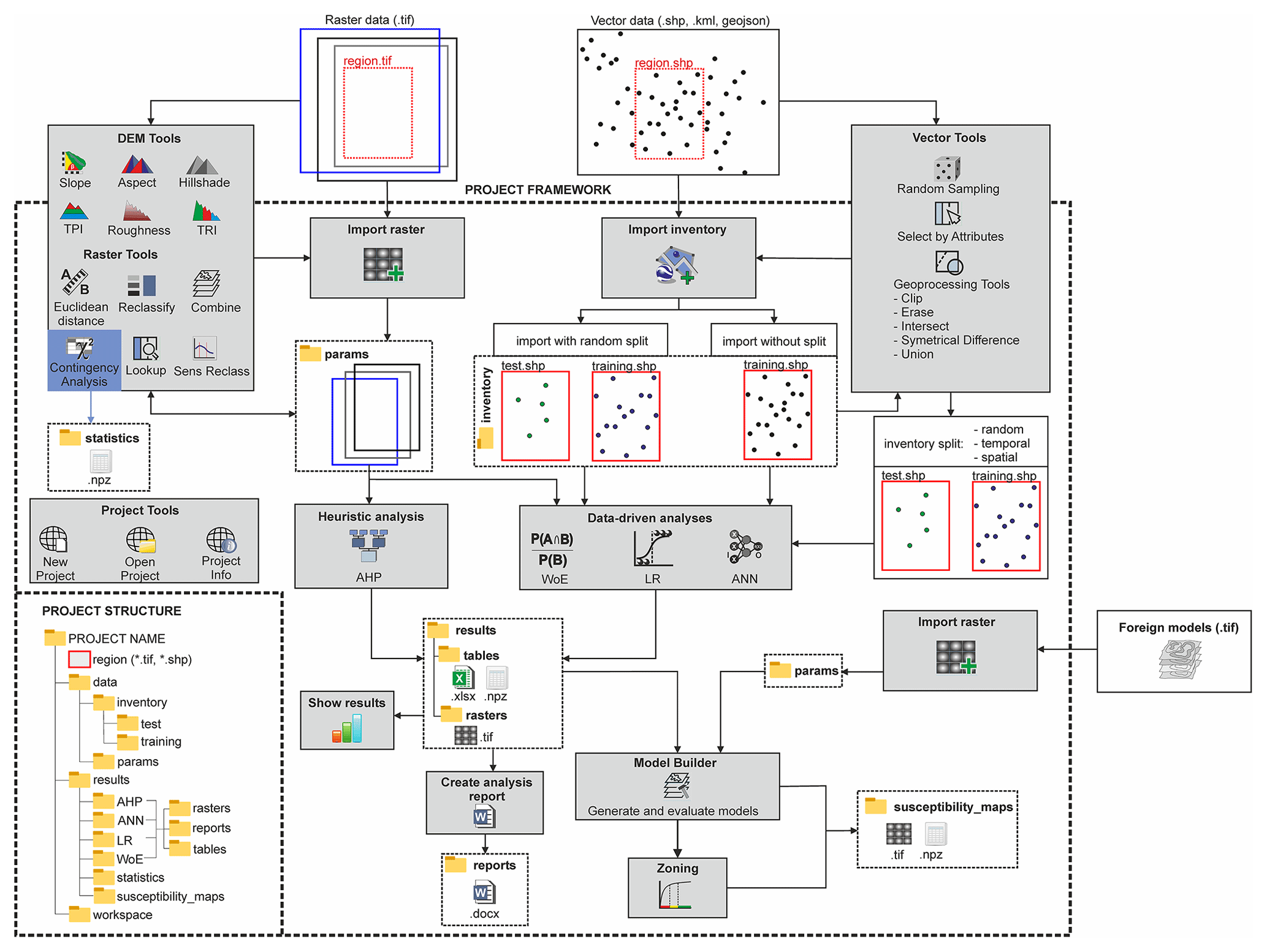
The logical workflow in Fig. 1 schematically sketches the working process with LSAT PM. The following sections briefly introduce the single steps of this workflow and their corresponding modules. More technical details are obtainable from the software documentation distributed stand-alone or as part of the installer package (see also Sect. 7).

Figure 1 Standardized project structure and the logical workflow of LSAT PM.

3.1 Project

After launching the software, the user can create a new or open an existing project. A project is a structured folder system that stores data with a specified spatial extent and spatial reference (region). The spatial extent and spatial reference need to be assigned on project creation manually or by selecting an already existing raster dataset as a project reference file (recommended).

The LSAT PM project has a standardized predefined structure, as shown in the bottom left of Fig. 1. The local project file overview (Catalog in Fig. 2) in the main GUI helps manage the project data by providing a data-type-dependent context menu.

3.2 Data import

Data import distinguishes between Import Raster and Import Inventory (Fig. 2). The first tool imports raster datasets considered to represent independent exploratory factors (features), and the second imports vector-based datasets for observational data representing inventory or labels.

The raster import tool ensures consistency by validating imported datasets against the project reference dataset (region). If not consistent with the project reference, the data get warped. This procedure is comparable to the concept of regions found in GRASS GIS and helps avoid processing errors due to specific resolution and spatial reference inconsistencies. The import procedure generates data copies; thus, original files remain unchanged.

Inventory import generally does the same for vector datasets as input. Additionally, it includes the random splitting of the dataset into training and test datasets. Using this option, the user can specify the percentage ratio of training and test datasets. The splitting option is not mandatory and skippable because inventory subsetting is possible later using one of the tools described in Sect. 3.3 (see also Fig. 1).

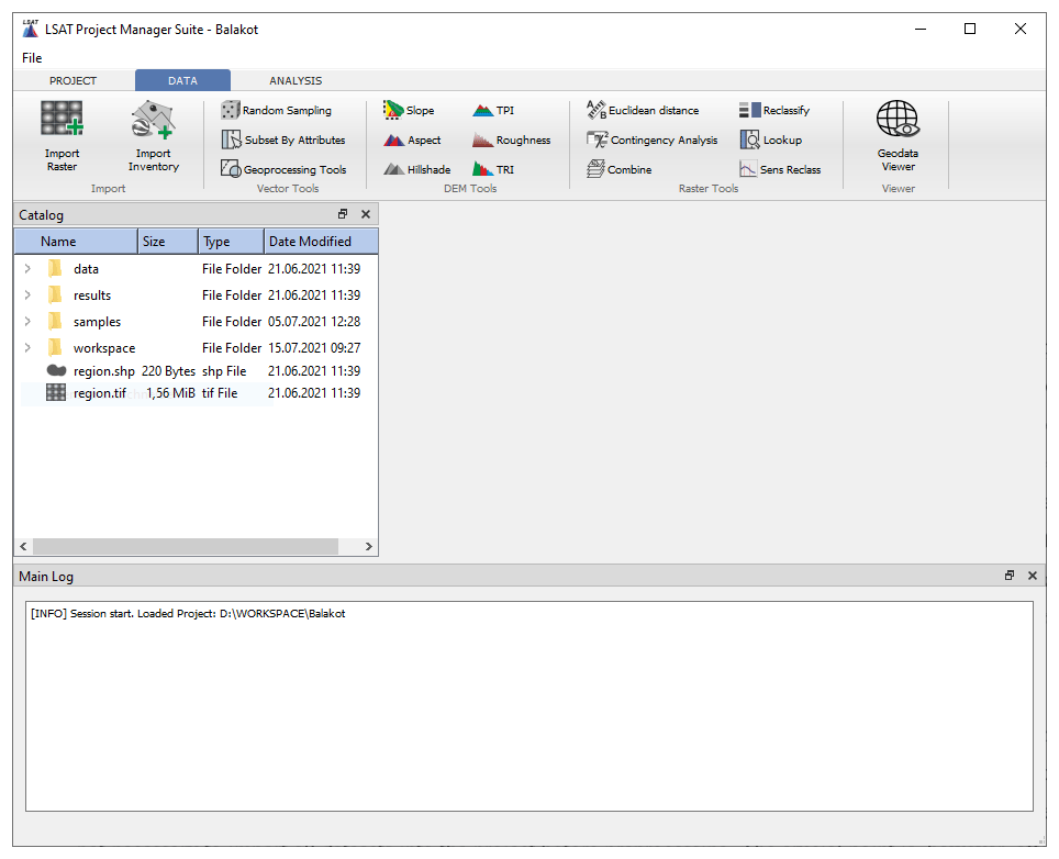
Figure 2 Main GUI with activated Data tab. The Data tab contains tools for data import, vector data processing, DEM tools, tools for raster processing, and a simple data viewer.

3.3 Data exploration and preprocessing

In the preprocessing step, we derive parameters and prepare the data according to the requirements of the upcoming analysis. Vector, DEM, and Raster Tools of LSAT PM (Fig. 2) aid this purpose.

Data subsetting is an essential technique to evaluate data-driven models using a test dataset not involved in the model's training, also known as cross-validation (e.g., Xu and Goodacre, 2018; Petschko et al., 2014; Chung and Fabbri, 2008). LSAT PM provides a palette of Vector Tools (Fig. 2) that supports the generation of inventory subsets based on random subsampling or feature attributes, e.g., the date (temporal split). Using Geoprocessing Tools in the same tool domain, the user can also subset the inventory based on spatial features (spatial split).

Digital elevation models (DEMs) serve as a basis for morphometric parameters such as slope, aspect, or TPI. DEM Tools (Fig. 2) derive basic morphometric features and generate raster data outputs from DEM raster datasets.

Raster Tools help perform basic raster operations and spatial analyses. Using the Combine tool, the user can combine several discrete raster datasets to generate a new raster dataset exhibiting unique conditions of higher complexity. Linear and point vector data (e.g., tectonic features, roads, streams, or point locations) are usually unsuitable as direct input for spatial analysis. However, their possible spatial effects are considerable via distance maps. The Euclidean distance tool generates a distance raster dataset based on input vector data.

Raster reclassification is a standard procedure in GIS analyses applied as value replacement in discrete datasets or binning of continuous datasets. Because WoE utilizes discrete data only, continuous raster data such as slope or distance rasters need a binning in the data preparation process. The Reclassify tool offers different classifiers such as equal intervals, quantiles, defined intervals, and user-defined values. Additionally, the Sensitivity Reclassification (Sens Reclass) tool provides a sensitivity analysis to find optimal cutoff thresholds (e.g., Torizin et al., 2017).

The Contingency Analysis tool performs the chi-square-based contingency analysis on raster-based categorical data, estimating the associations between the datasets based on Pearson's C, Cramer's V, and ϕ. It is the only tool that produces output in the subfolder statistics of the project results folder. The user can view the output contingency table via the Show results option from the Catalog's context menu.

All the above-presented tools apply to datasets in any location. Thus, the user can perform preprocessing steps before the data import.

3.4 Analyses

As already introduced in Sect. 2, LSAT PM implements heuristic and data-driven methods for LSA representing different categories (e.g., bivariate and multivariate). All of the methods have different levels of complexity, which need to be accounted for when choosing a specific analysis method. Table 1 briefly summarizes the corner points of the approaches such as category, supported data types, and complexity. The introduced complexity is a subjective measure that we assigned based on our experience evaluating criteria such as needed mathematical background, the complexity of data preparation, model structure and computation algorithm (transparency), and interpretability of the results. Due to the high degree of automation, the more complex methods allow running the analysis with its default settings without any adjustment and might therefore appear more straightforward. However, this first impression will vanish once the user encounters the advanced settings of the methods.

Table 1 Analyses included in LSAT PM and their specifications.

3.4.1 Weights of evidence

WoE is a bivariate statistical approach estimating the association between the observational data (dependent variable represented by the training landslide inventory) and a potential controlling factor (independent variable represented by, e.g., geological conditions). The analysis output is a raster of the specific controlling factor containing logarithmic log-likelihood weights, which characterize the relationship of discrete factor classes with a landslide occurrence. Individually weighted factors are then overlaid into a linear model to obtain the overall landslide susceptibility pattern (Torizin et al., 2017).

WoE in LSAT PM offers three different analysis modes: simple cross-validation, on-the-fly subsampling, and sampling with predefined samples. The default option is simple cross-validation (presupposes inventory split into training and test datasets). With this option, the model weight estimation runs once with the entire training dataset (no further subsampling). For on-the-fly subsampling, the weight estimation runs for several user-defined iterations, taking random samples (without replacement) of user-defined size from the training inventory. The estimated weights are mean values from all iterations. The analysis with predefined samples utilizes predefined sample datasets in a specified folder location. These predefined samples must be created beforehand by any subsetting algorithm introduced above (Sect. 3.3). The computed weights are mean values from all iterations, identical to the on-the-fly subsampling.

After the training, the result table and the weighted raster are automatically exported into the corresponding result folders. The results can be visualized immediately after the analysis through the WoE widget or later by calling the result viewer from the Catalog's context menu.

The model generation process is performed in the next step using the LSAT PM model builder module (see Sect. 3.5).

3.4.2 Logistic regression

Logistic regression (LR) is a multivariate statistical classification method to estimate relationships between the dependent variable and independent controlling factors. In contrast to WoE, LR analyzes the associations for all controlling factors at once and can utilize both continuous and discrete data as independent variables.

In LSAT PM, LR runs more automated than WoE. The user has to determine if the parameter is a discrete or continuous variable in the beginning. After that, the data preparation process runs automatically. The continuous datasets are scaled using a min–max scaler to the value range between 0 and 1; discrete datasets are transformed into binary dummy variables. All setting options for the logistic regression, e.g., regularization or solver algorithm, implemented in the sklearn library are adjustable to the user's needs in the advanced settings GUI. After the training, the result table and the prediction raster are automatically exported into the corresponding result folders.

Unlike WoE, the analysis output from multivariate LR already provides a multiparameter landslide susceptibility model.

3.4.3 Artificial neural network

ANNs are computer models inspired by biological neural networks. They consist of artificial neurons ordered in a network structure to simulate information processing, storage, and learning. The structure of an ANN usually consists of an input layer, one or more hidden layers, and an output layer. The number of hidden layers determines the depth of an ANN (e.g., Schmidhuber, 2015; Hernández-Blanco et al., 2019). This structure is also known as the multi-layer perceptron (MLP). The layers are composed of neurons in which the information processing takes place. Theoretically, the number of hidden layers and their neurons is unlimited. Thus, the network design is strongly dependent on the complexity and nonlinearity of the task and the available processing capacity. Most ANNs utilized in LSA are feed-forward networks, which have an MLP structure with usually one hidden layer (e.g., Ermini et al., 2005; Lee and Evangelista, 2006; Alimohammadlou et al., 2014).

The implemented module for an artificial neural network (ANN) has an experimental status and runs comparable to the LR. ANN can utilize discrete and continuous data. Additionally, the user can specify the ANN properties. Among others, these settings comprise the number of neurons in the layers, the number of hidden layers, the activation function, and the solver to use. The design of the network and the activation function selection constitute one of the most sensitive steps of the analysis with ANN. Despite reviewing numerous studies, we do not have a straightforward, practical recipe for designing the network yet. Therefore, the default settings do not represent the best practical approach but rather the defaults delivered with the sklearn library.

Nevertheless, the GUI and included data preprocessing provide easy and fast access to the capabilities given by the sklearn library and allow exploring the ANN performance for LSA. More technical information is obtainable from documentation of LSAT PM and sklearn library.

The data scaling process runs identically to the LR module. After the training process, the output raster defining the spatial probability of landslide occurrence is exported to the corresponding result folder.

3.4.4 Analytical hierarchy process

As a heuristic approach, the AHP is different from the data-driven applications explained above. The users must specify the weights, usually based on their general expertise (knowledge of geological processes) and specific knowledge about the investigation area. The weighting process is a pairwise comparison of the inputs at different hierarchical levels. For LSA, the AHP typically takes two hierarchical levels. The first level controls the class priorities inside multiclass parameters (e.g., raster values), and the second sets the priorities between the multiclass parameters (e.g., raster datasets).

The pairwise comparison is complex when working with parameters exhibiting many classes. The human ability to compare is limited to approximately seven objects, plus or minus two (Miller, 1956). Saaty (1977) considered this, proposing values between 1 and 9 in specifying the factor's importance. Therefore, in the preparation process, it is advisable to reduce the number of classes by generalization or subdivision in different hierarchical groups (e.g., Balzer et al., 2020). The latter will make the hierarchy more complex.

The advantage of pairwise ranking compared to simple ranking is the ability to verify the logical consistency of the decision mathematically. AHP uses the consistency ratio (CR) to indicate whether the introduced ranking is a logical inference or a random guess. Saaty (1980) recommends a CR under 0.1 for consistent assessment.

It is notable that some studies applying AHP for LSA use a hybrid approach combining bivariate methods with AHP (e.g., Kamp et al., 2008, 2010). In the hybrid approach, a data-driven bivariate approach applies to the first hierarchical level using, e.g., WoE. Afterward, additional expert-based weights derived from the AHP priority vector are applied to overlay the parameters to the model. Such an approach can preserve the crude generalization of the patterns in the first hierarchical level, making the analysis applicable to more detailed datasets. For the AHP part, the method becomes more applicable by involving the expert weights at a higher hierarchical level, which benefits more from general process understanding than detailed local knowledge.

Conversely, it also has implications for the bivariate analysis part. Using conditionally dependent parameters becomes less critical since experts adjust the parameter's contribution in the upper hierarchical level. However, the hybrid approach is only possible if a sufficient number of observations for the first data-driven step is available.

The implemented AHP is a pure expert-based tool supporting two hierarchy levels. The user has to perform the pairwise ranking for single parameter classes in the first step and the parameters in the second step. After the user has specified the class and parameter ranking, the analysis estimates the priority vector and generates a weighted overlay map. The result table and the weighted raster are automatically exported into the corresponding result folders. The resulting raster represents the final susceptibility map, similar to LR and ANN.

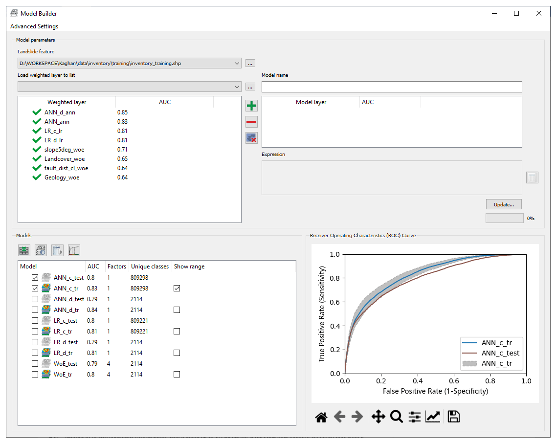
3.5 Model builder

The model builder (MB) is, in simple terms, a raster calculator with an integrated evaluation module. The algorithm behind the model evaluation is the receiver operating characteristics (ROC) curve – a technique to visualize and evaluate the classifier's performance (e.g., Fawcett, 2006) by depicting the ratio of the true positive rate (sensitivity) and the false positive rate (1-specificity). The area under the ROC curve (AUC or AUROC) provides a quantitative measure to compare the goodness of different models.

At the start, MB automatically searches and imports analysis results and existing models to the corresponding weighted layer and model collections, as shown in Fig. 3b and e. The user can specify which layers to include in the weighted overlay model by shifting the layers into the model layer collection (Fig. 3c). The model-generating expression is adjustable on demand. The default model-generating expression is a simple additive overlay of selected weighted layers.

MB performs the overlay according to the data-generating expression and uses the ROC curve to evaluate the model based on the specified landslide inventory dataset (Fig. 3a). Moreover, the evaluation procedure can be performed based on iterative random subsampling or predefined sample groups. The user can select these options in the advanced settings of MB.

Using the training inventory, the user evaluates the model fit. For the test dataset, the user evaluates the predictivity of the model on new data. Using iterative subsampling, users get an idea about the variance of the model based on different samples, which allows them to evaluate sampling errors (e.g., Torizin et al., 2018, 2021). The latter might be a helpful feature for interpreting evaluation results if the test datasets are comparably small. Exploring the variance of the training dataset in conjunction with the test ROC curve helps to understand whether the uncertainty of the model is the property of insufficient data (sampling error) or model accuracy (bias).

Moreover, the user can mix the model input layers (Fig. 3c) and adjust the generating expression (Fig. 3d). This flexibility allows the generation of hybrid models and model ensembles. Hybrid models combine different classifiers in one model, e.g., WoE for discrete data and LR for continuous data; model ensembles consist of different homogeneous models, e.g., LR and ANN. Here it is essential to note that weighted layers or models generated by different classifiers may exhibit different value ranges and need transformations when used together in a hybrid model or model ensemble. Through the model building expression, the user can implement those transformations instantly.

MB's model collection (Fig. 3e) lists all generated models and provides essential management to export models to GeoTiff and visualize the corresponding ROC curves (Fig. 3f). All generated models include metadata with information on model input layers and applied model-generating expression, making the results more reproducible. The Model Info function provides access to the model's metadata.

Figure 3 Model builder GUI with its integral parts: a – landslide inventory collection; b – weighted layer collection; c – model layer collection; d – model-generating expression; e – model collection; f – ROC curves.

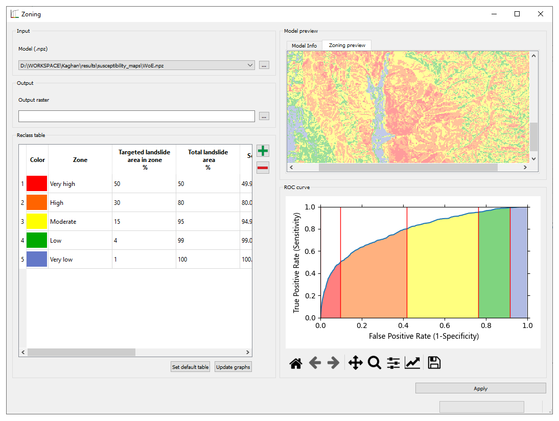
3.6 Zoning

The zoning procedure applies to all models generated or evaluated with LSAT PM. It uses the model's ROC curve to aggregate the model output with many different landslide susceptibility index (LSI) values to a legible map with few susceptibility zones. The zoning procedure follows the general concept proposed by Chung and Fabbri (2003). The basic idea is to specify class boundaries using cumulative landslide area over ranked unique condition classes representing the cumulative study area. Chung and Fabbri (2003) proposed using the success rate depicting cumulative landslide area over the ranked cumulative area considered susceptible. However, it also partly applies to ROC curves since the y axis representing the true positive rate corresponds to the cumulative landslide area. The x axis in the ROC curve is the false positive rate depicting cumulative study area without landslide areas: in other words, areas that have been regarded as susceptible but do not contain landslide areas. Thus, the cumulative sum over the x axis is only an approximation of the total study area, which is sufficiently accurate if the landslide areas are neglectable compared to the total area (e.g., when working with point data inventories in large regions). However, it also means that the accurate zone proportions cannot be directly estimated from the ROC curve graph if landslide areas are considerably large. Therefore, the total area values in the reclass table represent only approximations for zone area proportions.

Nevertheless, this discrepancy does not affect the implemented classification because we restrict the input to the proportion of cumulative landslide areas within a zone. The specified cumulative landslide area value relates to the rank position of the specific unique condition that exhibits a specific landslide susceptibility index (LSI). The LSI is finally used to set the classification threshold for the class boundary. The zone areas in the attribute table of the output zoning raster are computed directly from the raster values and represent accurate values.

There are no well-established standards for the number of zones or the definition of zone boundaries. In our case studies (e.g., Torizin et al., 2017, 2018), we used the proportions of 50 % of all landslide pixels in the very high, further 30 % for the high, 15 % for the moderate, 4 % for the low, and about 1 % for the very low susceptibility zone (Fig. 4). These thresholds apply when the user selects the default table.

Alternatively, the user can use the Reclassify tool to aggregate the model to zones with customized thresholds directly on the model's LSI or probability values.

Figure 4 Zoning tool with applied default classification.

4 Application example

4.1 Test data

A dataset to test the functionalities of the software is available from https://doi.org/10.5281/zenodo.5109620 (Georisk Assessment Northern Pakistan, 2021). The example or test dataset is an excerpt of the data collected in the German–Pakistani technical cooperation project Georisk Assessment Northern Pakistan (GANP) carried out by the Federal Institute for Geosciences and Natural Resources and Geological Survey of Pakistan (e.g., Torizin et al., 2017). The dataset covers about 664 km², including parts of the Kaghan and Siran valleys in Khyber Pakhtunkhwa (KP), northern Pakistan (Fig. 5a). Table 2 and Fig. 5 provide an overview of the test data.

Table 2 Overview of the datasets in the test data.

A severe Kashmir earthquake struck the region on 8 October 2005, with a moment magnitude of 7.8, triggering thousands of landslides. The collected landslide inventory results from the visual interpretation of optical satellite images available through Google Earth, which, during the data acquisition, consisted mainly of imagery from Quickbird (up to 0.60 m ground resolution), IKONOS (∼4 m ground resolution), SPOT (SPOT5 about 5 m ground resolution), and Landsat (15 m ground resolution) (Torizin et al., 2017). In total, the landslide inventory includes 3819 events for the test area depicted as polygons. Landslide sizes range from about 12 to about 88 444 m², representing the depletion area of the landslides (as far as it was possible to determine by visual interpretation of imagery).

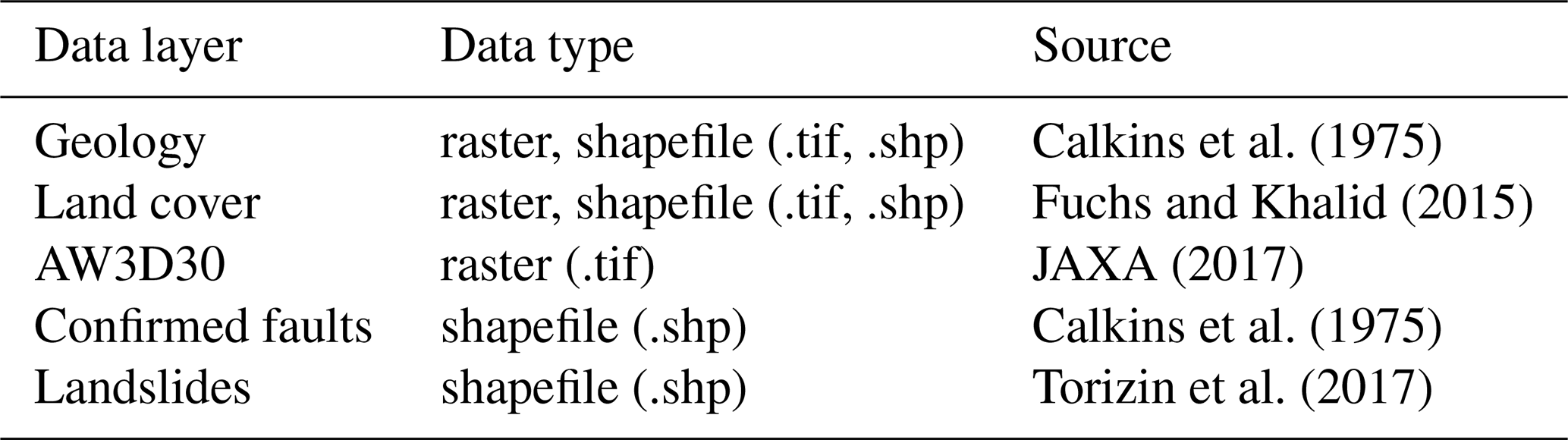
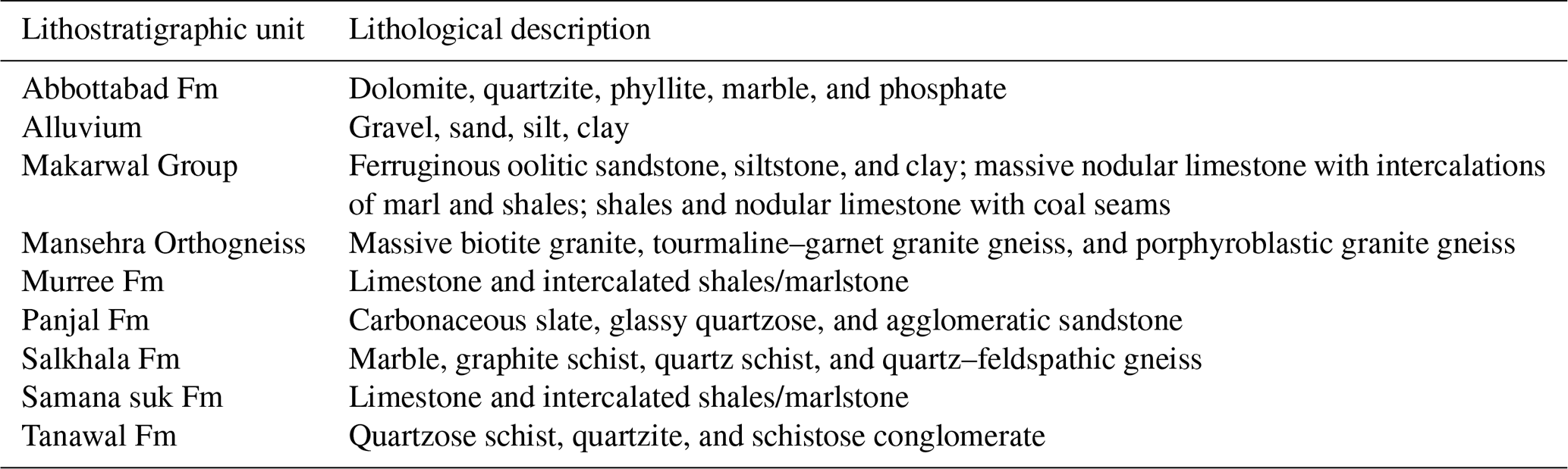
The digital elevation model is the ALOS global digital surface model (AW3D30) (JAXA, 2017) with a ground resolution of approximately 30 m (Fig. 5a). The geological information and the tectonic features (faults) were derived from the geological map of Calkins et al. (1975) (Fig. 5d and Table 3). The land cover results from the supervised classification on Landsat imagery performed by Fuchs and Khalid (2015) (Fig. 5c). The test dataset contains geology and land cover in raster and vector data formats. Note that the vector formats for parameters cannot be directly used for analysis in LSAT PM yet. However, the vector datasets may help test the Vector Tools (e.g., subsetting landslides based on specific geology or land cover class).

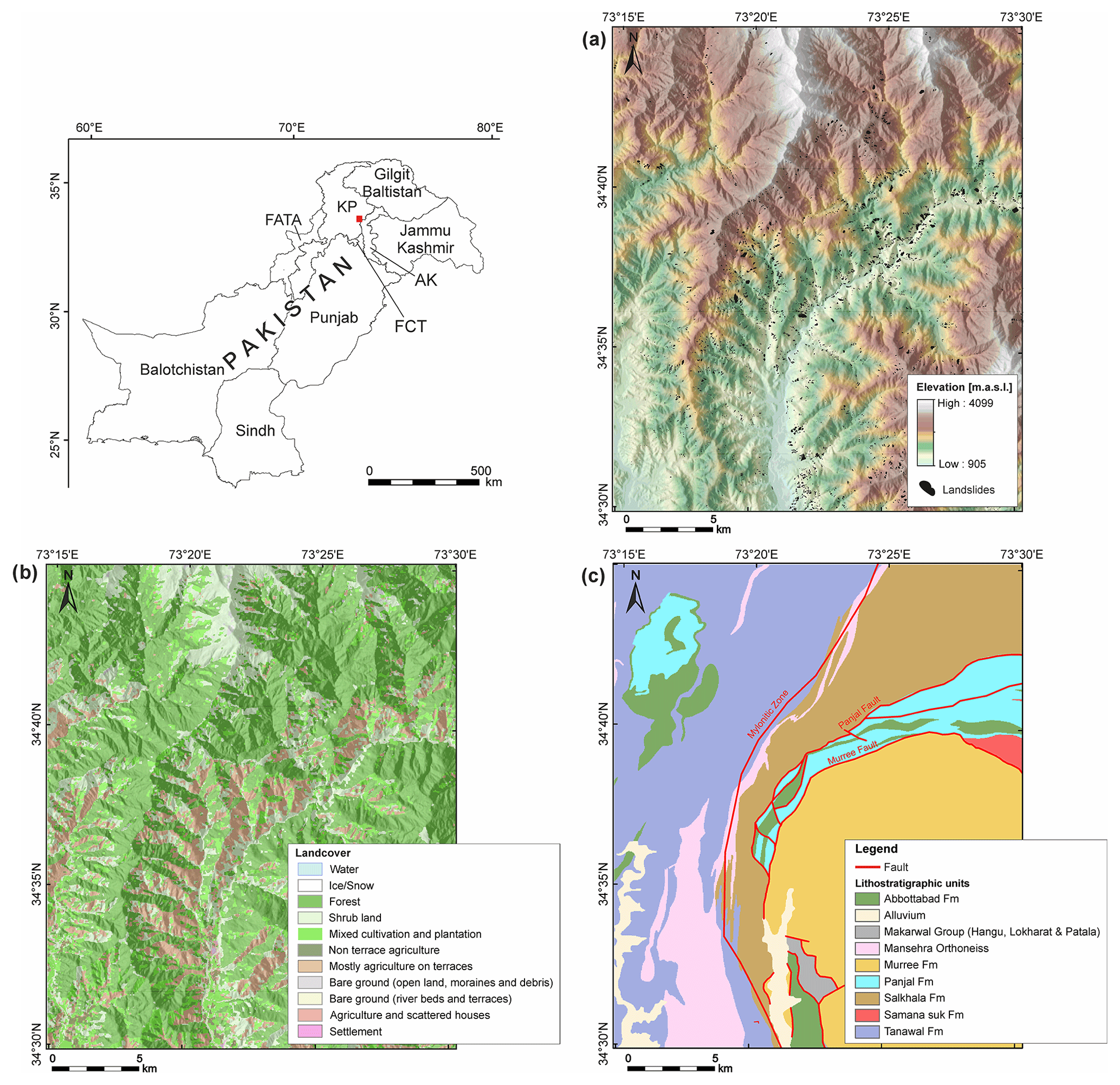
Figure 5 Example dataset. (a) AW3D30 with landslide inventory; (b) land cover; (c) geology with prominent (confirmed) faults.

Table 3 Lithostratigraphic units of the geology layer with lithological description (after Calkins et al., 1975).

4.2 Analysis workflow

In the following example, we use the test dataset to showcase how to perform a simple LSA with WoE, LR, and ANN in LSAT PM and compare the model outputs. We skip the analysis with AHP in this example due to its high subjectivity and our lacking detailed knowledge about the investigation area.

Figure 6 shows the principal workflow of the performed steps. The first seven steps cover the project creation, data import, and first preprocessing of the imported data, such as computation of the slope and Euclidean distance as well as binning of continuous data in categories suitable for WoE. In step 8, the contingency analysis measures associations among discrete datasets based on chi-square metrics. The utilization of strongly correlated datasets may lead to incorrect estimation of the factor's contribution and inflation of the estimated probability values (e.g., Agterberg and Cheng, 2002).

In step 9, we prepare the data to evaluate model uncertainties. Therefore, we compared the size of the landslide training and test datasets. In step 2, the selected split option subdivided the imported landslide inventory into training, containing 2674 events, and the test dataset with 1146 events. The latter corresponds to approximately 43 % of the training dataset. To estimate the sample-size-dependent model variance, we generated 100 random subsamples from the training dataset of the test dataset's size with the Random sampling tool. To make the results reproducible, we set the random seed to 42. The training and test inventory are random subsamples from the same dataset. Therefore, they represent the same spatial distribution but with a different mean sampling error (MSE) related to the sample size. Torizin et al. (2021) showed that evaluation of the model performance based on a test inventory of a smaller size than a training inventory must consider this for correct interpretation of the results. Evaluation with the 100 subsamples of the same size as the test inventory but derived from the training inventory dataset has two implications. First, all training events are known to the model and follow the same spatial distribution as the complete training inventory. Variations in model performance on these datasets define the MSE, which is expected to be in a similar range by evaluating the model with a test dataset of the corresponding size. Thus, the shape of the ROC curve and AUC value should fall within the MSE range if the model generalizes well without significant overfit.

Figure 6 Workflow applied to the test dataset.

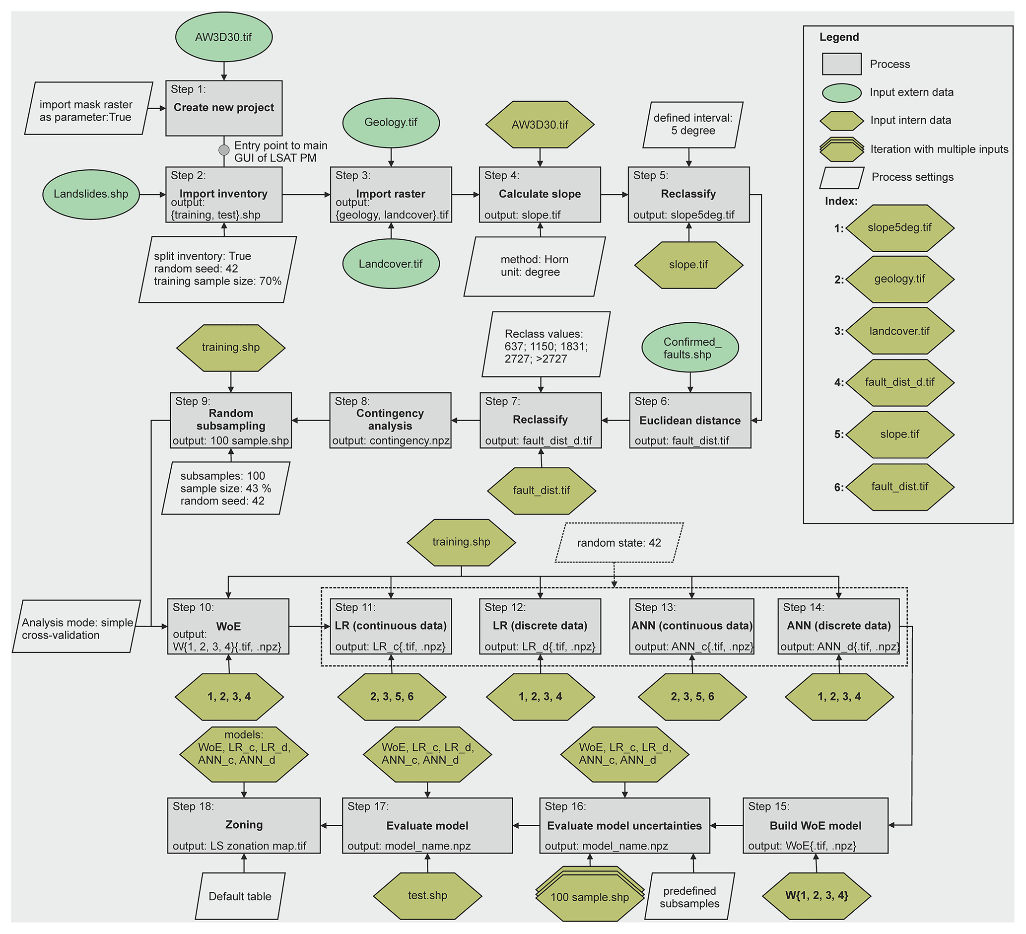
Steps 10 to 14 cover the analysis part. We calculated the WoE, LR, and ANN models in different ways to contrast the approaches. The WoE can utilize only discrete data; therefore, we used the classified and initially discrete data to generate the weighted layers. The LR and ANN support usage of both continuous and discrete data. Therefore, we used the capability of both approaches to utilize discrete and continuous data and generated two models for LR and ANN, respectively. The first, marked with the _c suffix, utilizes both data types, and the second, marked by the _d suffix, utilizes only discrete datasets as used in WoE.

Step 15 is the generation of the WoE model in MB by adding single weighted layers. To better compare the results from WoE with results from ANN and LR, we adjusted the model-generating expression to transform the log likelihoods of the WoE model into probabilities by applying the logistic function (see also Appendix A for details). In step 16, models uncertainties related to sampling error were evaluated in MB using 100 predefined subsamples generated in step 9. With this, the ROC curve is iteratively computed for every subsample. In the consecutive step, the models were evaluated with the test dataset not involved in the training process before, thus representing new data. Finally, we used the ROC curve from the test dataset to generate legible susceptibility maps consisting of five susceptibility zones (default table, see Sect. 3.6) using the Zoning tool.

4.3 Results and discussion

While the first steps of data import and preparation, such as reclassing usual GIS functionalities, are trivial and partially described in Sect. 3, the contingency analysis in step 8 is worth examining. The results of the contingency analysis are saved in NumPy archive format (.npz) in the folder statistics.

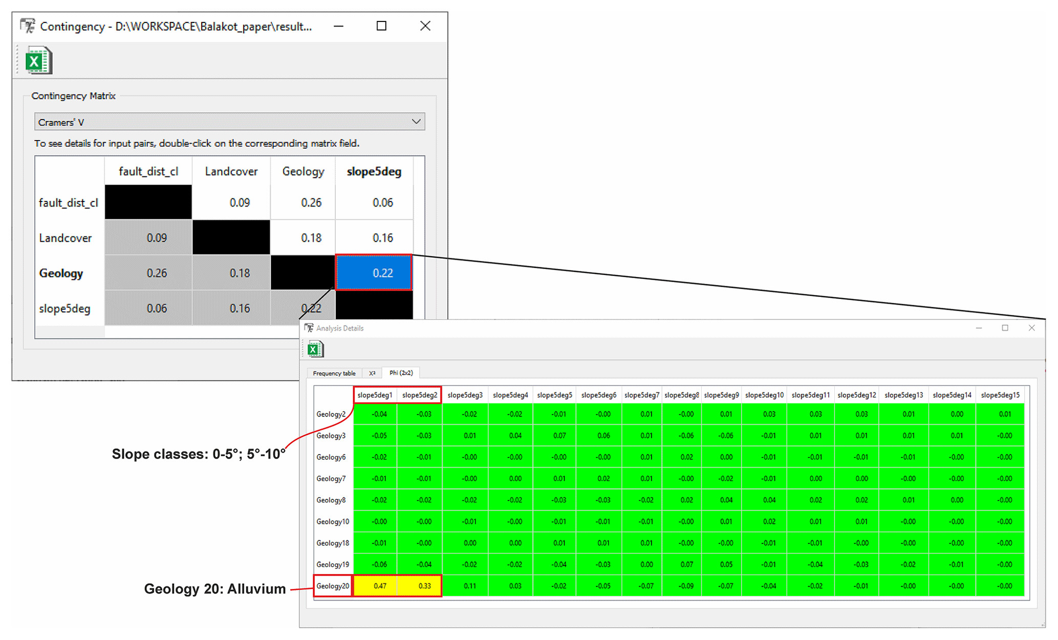
Figure 7 Example for the contingency result output: the first window represents an allover contingency matrix between multiclass parameters based on Cramer's V. On double-click, the detailed contingency between Geology and slope5deg is callable.

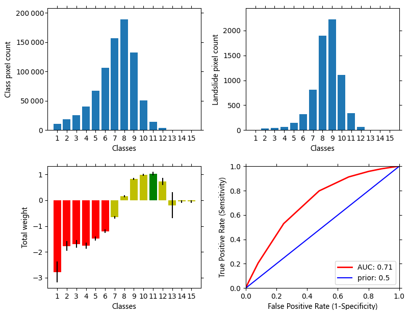
Figure 8 Graphical result output of WoE analysis for the simple cross-validation mode. Note that bar plots change to box or violin plots for other analysis modes such as on-the-fly subsampling.

Figure 9 Evaluation and comparison of the models in MB.

The analysis output consists of different tables (Fig. 7). The first result table shows the overview for all involved parameters based on Cramer's V and Pearson's C. Both metrics are estimates for the general association of the multiclass datasets. However, they do not allow determining in detail whether, e.g., a moderate association comes from several moderately associated classes or as an average estimate from one strongly associated class pair among other non-correlated discrete classes. Therefore, an additional ϕ metric based on the 2×2 contingency table is callable on double-click on the specific matrix cell, providing more detail for the specific parameter pair. It highlights the pairwise association among single variable class pairs. The tables are colored to emphasize the strength of association: green for no to marginal association, yellow for the moderate association, and red for the strong association. In Fig. 7, it is clear that while most classes of geology and classified slope layer are not correlated, a moderate association is present for alluvial deposits forming the valley fillings and slope between 0 and 10^∘.

In the WoE tool, the user can explore the associations among the single factor and the occurrence of the events. The results viewer contains all relevant information on the modeling process. The result table represents discrete class area distribution, corresponding landslide pixel frequencies in those classes, computed weights, variance, standard deviation, posterior probability values, and expected observations. The default output raster with suffix _woe derives from the table column weights. The included graphical representation of the results provides a quick overview of class and landslide pixel distributions, weights, and corresponding ROC curves (Fig. 8). WoE results can be exported as an analysis report in MS Word format that concisely represents the relevant features.

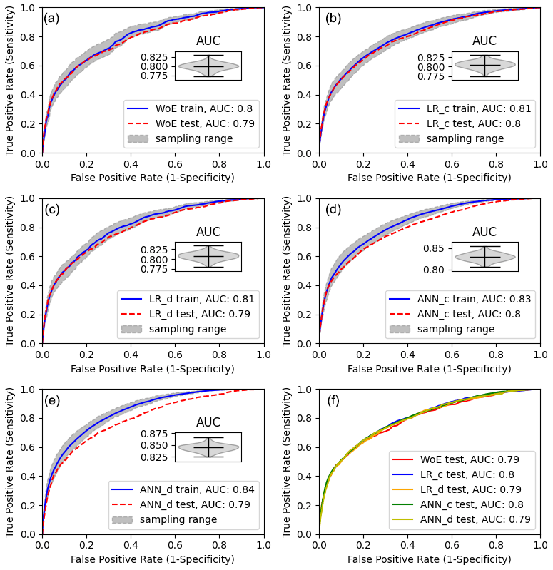
Figure 10 ROC curves for the different models. The greyish band marks the model uncertainty based on the MSE. The insert in (a)–(e) shows the corresponding distribution of AUC values for the utilized samples.

Outputs from LR and ANN analyses are compact. Among the involved parameters and model settings, LR results highlight the estimated coefficients and some informational metrics helping to find a trade-off between model complexity (number of explanatory variables) and explained variance such as the Akaike information criterion (AIC) and Bayesian information criterion (BIC), as well as the AUC of the corresponding ROC curve. The experimental ANN provides metadata on model inputs and settings, model score, and AUC value. For both graphical result output and corresponding analysis, reports are not implemented yet (see also Sect. 5).

The evaluation of model uncertainties in step 16 and model evaluation with test data in step 17 suggest that all three approaches deliver comparably good models. Although MB allows appropriate management for comparing the models (Fig. 9), we used customized scripts for Figs. 10, 11, and 13 (see Sect. 8) to showcase additional post-processing possibilities based on LSAT PM outputs.

To aggregate the results to a compact and legible figure (Fig. 10) providing some additional features not included in MB yet, we utilize the outputs of the MB. Figure 10 shows the performance of the models based on the predefined subsamples.

Figure 11 Pairwise comparison of the predicted landslide susceptibility patterns.

The greyish error band around the mean ROC curve indicates the MSE. As we can see from the violin plot inserts in Fig. 10a–e, the variance of the corresponding AUC values shows the normal distribution. At first glance, ANN_d and ANN_c models have the best training performance with AUCs of 0.84 and 0.83, followed by LR_c with an AUC of 0.81. WoE and LR_d models show the worst training performance (AUC of 0.80). For the model evaluation on test data, we see that for the WoE, LR_d, and LR_c, the test ROC curve is within the expected MSE. For ANN_c and ANN_d, however, the test performance is significantly lower. In this case, we can interpret this as an overfit of the models. Using discrete variables in ANN_d, we introduced additional degrees of freedom compared to the ANN_c model; therefore, overfitting is more prominent in the ANN_d model. The reason is the flexibility of the ANNs with multiple neurons to also fit nonlinear data relations, which might be an advantage but at the same time a significant uncertainty source. Thus, if we had aimed to optimize the susceptibility map with ANN, we would need to review the network design or the number of iterations in the network training process to prevent overfitting. At this point, it is worth noting that imbalanced samples can also cause comparable effects. When using polygon landslide data, the imbalance may develop from rare large landslides appearing only in the training or the test inventory. Although this affects all model types, flexible ANNs might suffer more than, e.g., WoE. The solution would be to check the distributions of the training and test landslide datasets and, if imbalances are present, to generate balanced samples by, e.g., randomly drawing pixels from landslide areas instead of using them as a whole.

Because the interpretation of ANN results is not intuitive, we would generally recommend a parallel application of a multivariate linear model and ANN to see how much nonlinearity is introduced by the ANN and how it affects the model generalization capabilities.

Further, looking at the test ROC curves of all models (Fig. 10f), we see that the predictivity of the models is comparable with minor advantages for models utilizing continuous datasets. Thus, given the simple study design and available data, the models are equivalent alternatives from the statistical point of view. However, although the ROC curve provides a quantitative measure for classifier performance, as any statistical measure, it is not suitable for evaluating the model's reliability (e.g., Rossi et al., 2010). As we can demonstrate here, models with equivalent AUCs can exhibit substantially different susceptibility patterns. How meaningful those patterns are is beyond the statistical analysis capabilities and has to be verified based on other sources of information.

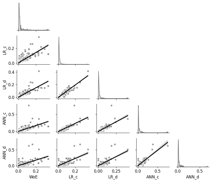
We compare the susceptibility models in a pair plot to evaluate the differences in obtained susceptibility patterns. The pair plot in Fig. 11 visualizes the pairwise pixel-by-pixel comparison of the model values. The matrix diagonal shows the distribution of the model values (marginal probabilities). In contrast, the scatter plots in the lower matrix corner of Fig. 11 show the covariance of the value pairs overlain by linear regression to emphasize the trend. The pairwise comparison reveals general linear relation for all models with better comparability for the multivariate models ANN and LR but substantial differences in detail.

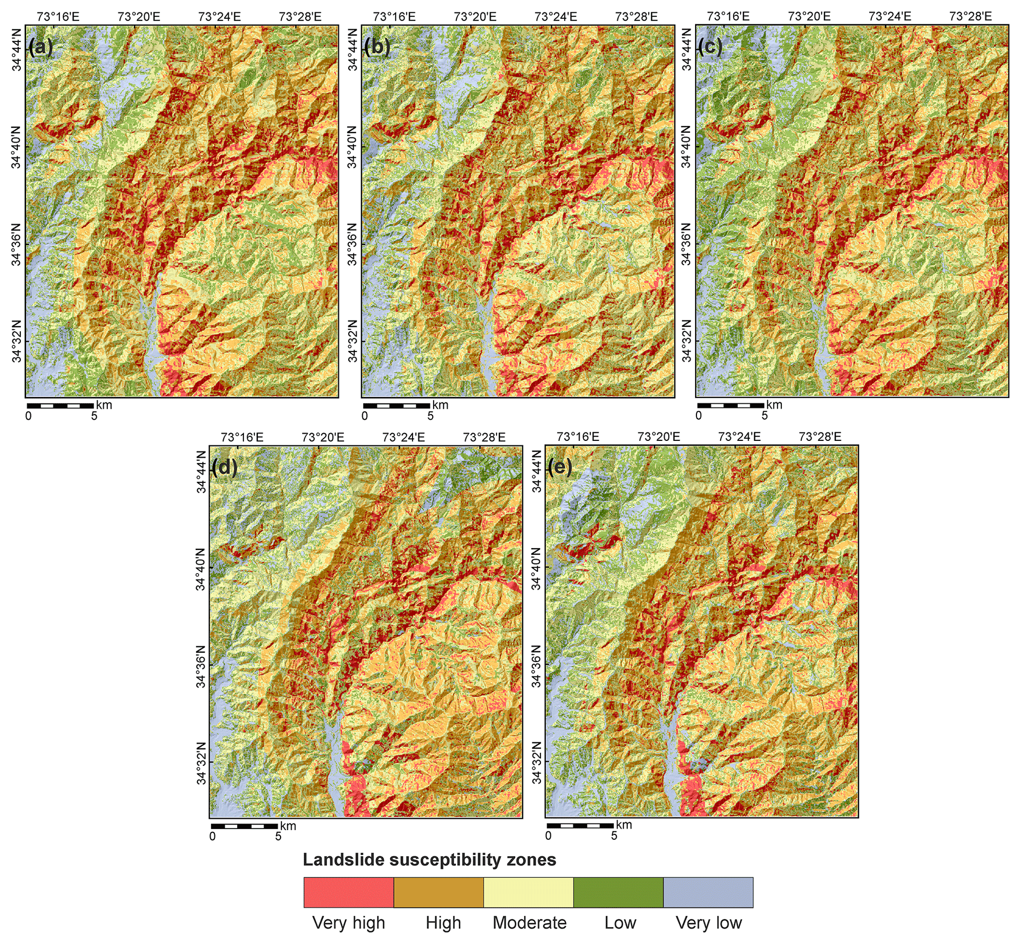
Figure 12 Landslide susceptibility zones based on different models. (a) WoE. (b) LR_d. (c) LR_c. (d) ANN_d. (e) ANN_c. Very high contains about 50 %, high about 30 %, moderate about 15 %, low about 4 %, and very low about 1 % of all landslide pixels.

Figure 13 Susceptibility zone distributions for the susceptibility models. The values in columns show the number of pixels within the zones.

We wanted to see how these differences affect the final zonation and compared the models using simple class frequency statistics after the zonation procedure. Figure 12 shows the landslide susceptibility maps after zonation with default values introduced in Sect. 3. In Fig. 13, the classified models are compared regarding their pixel counts within the susceptibility classes. While the highest susceptibility class containing 50 % of all landslide pixels shows minor differences, they become more significant in the lower susceptibility zones.

5 Conclusions and outlook

In this paper, we introduced LSAT PM that provides a framework for applying and evaluating knowledge- and data-driven spatial binary classification methods, and we demonstrated in part its capabilities based on a real-world test dataset. The given presentation is not exhaustive but provides a general idea of using the software.

Summarizing the capabilities of LSAT PM, we can emphasize that the project-based modular framework allows efficient data management at all steps of the LSA. The implemented logs on performed processing steps and metadata collection increase transparency and reproducibility and allow easy sharing of the modeling results, e.g., in working groups. At the same time, we tried to keep as many degrees of freedom as possible in the modeling procedures, providing users with not a fixed pipe but a toolkit that allows for flexible study designs. Thus, the preprocessing, analysis, and post-processing steps are performable according to the user's choice.

The MB module of LSAT PM implements functionalities allowing for practical evaluation of model uncertainties related to common sampling errors. Further, it provides a convenient way to compare models generated by the implemented algorithms and foreign models. The implemented raster calculator supports the generation of hybrid models and model ensembles.

LSAT PM targets a broad user profile. It provides access to LSA state-of-the-art methods for users beyond the academic community. Users with limited programming and scripting skills can perform analyses and explore the results via convenient GUI or export the results to other applications allowing further post-processing. Skilled users can also benefit from implemented standards and quickly enhance the analysis outcomes stored in NumPy archive format by own scripts, as we have shown in Sect. 4. This versatility makes LSAT PM well suited for educational purposes at all levels.

Of course, there is always room for improvement. Therefore, the LSAT PM is subject to continuous further development. We intend to implement additional and improve existing methods, e.g., improve the AHP and machine learning workflows. Especially for the latter, we intend to implement additional features to visualize the results and increase the interpretability of the model outputs. We intend to implement GPU support to perform better on massive datasets in machine learning methods. Also, some management features, such as a plugin builder tool that would support the easy implementation of customized plugins into the LSAT PM framework, are under preparation. Software documentation continuously updates with the ongoing development and will be extended by short video tutorials introducing the work with LSAT PM.

With the open-source approach, we would like to encourage interested scientists to join the development by introducing and discussing new ideas and sharing experience in spatial modeling of landslides and scientific programming in general.

Appendix A: Supporting information for weights of evidence

WoE uses Bayes' rule to estimate the conditional probability of an event based on prior knowledge and a set of pieces of evidence. Prior knowledge in terms of prior probability usually represents the average expectation of an event given a study area. For the raster-based analysis, the prior probability is calculated as the number of event pixels divided by the total pixels in the study area. Thus, the prior probability follows a uniform distribution over the entire study area (e.g., Torizin, 2016). We update the prior probability by weighted evidence factors, which we assume to be conditionally independent. For the spatial analysis, the factors characterize how much the probability value in a specific location is higher or lower than the prior probability. The updated probability is called the posterior probability (e.g., Teerarungsigul et al., 2015). The performed knowledge update cannot find new events but rather redistributes the probability density patterns conserving the total events (e.g., Agterberg and Cheng, 2002; Torizin, 2016). Thus, given the conditional independence of evidential patterns, we should obtain (approximately) the number of initial event pixels when summing up all pixels of the posterior probability raster. In practice, complete conditional independence of evidential patterns is rare. Therefore, using many factors may cause inflation of posterior probability by occasional double counting of the effects (Agterberg and Cheng, 2002). The latter sets a general requirement to perform a contingency analysis (e.g., based on χ² metrics) to estimate possible associations between evidence patterns.

In WoE, the weights for specific evidence patterns derive from the Bayes' rule formulation in logarithmic odds notation (e.g., Bonham-Carter et al., 1989; Bonham-Carter, 1994), considering the evidence as a binary pattern for the presence or absence of a specific feature. For multiclass datasets, the computation is done as if the dataset consists of several binary dummy variables. However, the straightforward analysis allows the weight calculation for multiclass datasets in one table without generating binary dummy variables explicitly. The weight calculation for a particular raster cell in a binary pattern distinguishes two cases. First, if the particular feature class C is present, then the logit is given by

$$\begin{array}{}\text{(A1)}& w^{+}={\log }_{\mathrm{e}}\left({\displaystyle \frac{P\left\{C\mathrm{|}E\right\}}{P\left\{C\mathrm{|}\stackrel{\mathrm{‾}}{E}\right\}}}\right).\end{array}$$

Otherwise, the logit is given by

$$\begin{array}{}\text{(A2)}& w^{-}={\log }_{\mathrm{e}}\left({\displaystyle \frac{P\left\{\stackrel{\mathrm{‾}}{C}\mathrm{|}E\right\}}{P\left\{\stackrel{\mathrm{‾}}{C}\mathrm{|}\stackrel{\mathrm{‾}}{E}\right\}}}\right),\end{array}$$

where P{C|E} is the conditional probability of C (feature) given E (event), $P\mathit{\left\{}C\mathrm{|}\stackrel{\mathrm{‾}}{E}\mathit{\right\}}$ is the conditional probability of C given $\stackrel{\mathrm{‾}}{E}$ (no event), $P\mathit{\left\{}\stackrel{\mathrm{‾}}{C}\mathrm{|}E\mathit{\right\}}$ is the conditional probability of $\stackrel{\mathrm{‾}}{C}$ (no feature) given E, and $P\mathit{\left\{}\stackrel{\mathrm{‾}}{C}\mathrm{|}\stackrel{\mathrm{‾}}{E}\mathit{\right\}}$ is the conditional probability of $\stackrel{\mathrm{‾}}{C}$ given $\stackrel{\mathrm{‾}}{E}$.

The weight notations w⁺ and w⁻ do not represent the mathematical sense of the values but the feature class presence (positive) and absence (negative) in the given raster cell.

With this formulation, positive logit values suggest a positive effect of the given variable, negative logits indicate a negative effect, and logits with a zero value indicate no effect. Thus, the latter does not modify the prior probability.

The posterior logit z is obtainable from weighted layers w_i (e.g., Barbieri and Cambuli, 2009; Torizin, 2016) as

$$\begin{array}{}\text{(A3)}& z=\text{PriorLogit}+\sum _{i=\mathrm{1}}^n{w}_i,\end{array}$$

where n is the number of weighted layers (evidence), and w_i is the ith weighted layer. The PriorLogit is

$$\begin{array}{}\text{(A4)}& \text{PriorLogit}={\log }_{\mathrm{e}}\left({\displaystyle \frac{\frac{\mathrm{total}\mathrm{landslide}\mathrm{pixel}}{\mathrm{total}\mathrm{area}\mathrm{pixel}}}{\mathrm{1}-\frac{\mathrm{total}\mathrm{landslide}\mathrm{pixel}}{\mathrm{total}\mathrm{area}\mathrm{pixel}}}}\right).\end{array}$$

To convert the logit formulation to posterior probability, we use the logistic function:

$$\begin{array}{}\text{(A5)}& p_{\mathrm{post}}={\displaystyle \frac{\mathrm{1}}{\mathrm{1}+e^{-z}}}.\end{array}$$

The sum of the weighted layers from Eq. (A3) is the default output in the LSAT PM model builder for WoE models. It is already sufficient to obtain the relative susceptibility pattern needed for evaluation. To obtain a model with probability values, the user should first compute the prior logit and modify the model-generating expression in the model builder according to Eq. (A5). Necessary information on the total number of landslide pixels and the total number of pixels in the study area is obtainable from the result table of any weighted layer. We recommend exporting the result table to Excel and conducting the simple side calculation as shown in Eq. (A4).