the Creative Commons Attribution 4.0 License.
the Creative Commons Attribution 4.0 License.
 | 01 Apr 2022
Simulation of organics in the atmosphere: evaluation of EMACv2.54 with the Mainz Organic Mechanism (MOM) coupled to the ORACLE (v1.0) submodel
Simon F. Reifenberg
Vinod Kumar
Bruno Franco
Matthias Kohl
Domenico Taraborrelli
Sergey Gromov
Sebastian Ehrhart
Patrick Jöckel
Rolf Sander
Veronica Fall
Simon Rosanka
Vlassis Karydis
Dimitris Akritidis
Tamara Emmerichs
Monica Crippa
Diego Guizzardi
Johannes W. Kaiser
Lieven Clarisse
Astrid Kiendler-Scharr
Holger Tost
Alexandra Tsimpidi
An updated and expanded representation of organics in the chemistry general circulation model EMAC (ECHAM5/MESSy for Atmospheric Chemistry) has been evaluated. First, the comprehensive Mainz Organic Mechanism (MOM) in the submodel MECCA (Module Efficiently Calculating the Chemistry of the Atmosphere) was activated with explicit degradation of organic species up to five carbon atoms and a simplified mechanism for larger molecules. Second, the ORACLE submodel (version 1.0) now considers condensation on aerosols for all organics in the mechanism. Parameterizations for aerosol yields are used only for the lumped species that are not included in the explicit mechanism. The simultaneous usage of MOM and ORACLE allows an efficient estimation of not only the chemical degradation of the simulated volatile organic compounds but also the contribution of organics to the growth and fate of (organic) aerosol, with the complexity of the mechanism largely increased compared to EMAC simulations with more simplified chemistry. The model evaluation presented here reveals that the OH concentration is reproduced well globally, whereas significant biases for observed oxygenated organics are present. We also investigate the general properties of the aerosols and their composition, showing that the more sophisticated and process-oriented secondary aerosol formation does not degrade the good agreement of previous model configurations with observations at the surface, allowing further research in the field of gas–aerosol interactions.
- Article
(7775 KB) - Full-text XML
-
Supplement
(574 KB) - BibTeX
- EndNote


Volatile organic compounds (VOCs) play a pivotal role in the atmosphere by constraining the total oxidant level and serve as precursors of ozone (O3), carbon dioxide (CO2) and secondary organic aerosols (Heald and Kroll, 2020). Due to the complexity of the chemistry of VOCs, a comprehensive and explicit representation thereof is mostly still missing in global and regional model simulations (Heald et al., 2005). To capture this full complexity, model simulations would become rather computationally expensive and slow in performance. However, missing this complexity also substantially limits the current understanding of the budget of secondary pollutants, e.g. O3 and aerosols. The challenges involved are twofold: (1) understanding and including the chemical degradation pathways and (2) representing all other influencing processes (e.g. deposition, multiphase chemistry) in already complex global and regional models.
A chemical mechanism that stands out for size and detailed oxidation of many important VOCs is the Mainz Organic Mechanism (MOM, Sander et al., 2019). MOM represents the chemistry of alkanes, alkenes, terpenes (isoprene and monoterpenes) and monocyclic aromatics. The mechanism has been employed to study the impact of isoprene OH recycling above pristine tropical forests (Taraborrelli et al., 2012), oxidation of monoterpenes as a source of HO2 (Hens et al., 2014; Mallik et al., 2018) and the influence of aromatics on tropospheric ozone (Taraborrelli et al., 2021). Furthermore, MOM has been used with extensions in order to simulate product yields of β-caryophyllene oxidation (van Eijck et al., 2013), the oxidation of alkyl amines and formamide as source of isocyanic acid HNCO (Rosanka et al., 2020), the atmospheric losses of stabilized Criegee intermediates (Vereecken et al., 2017), and the most recent OH-recycling mechanisms in isoprene oxidation (Novelli et al., 2020). However, a full evaluation of the VOC distribution predicted by MOM in a global numerical model has not been published.
Furthermore, a more detailed chemical mechanism, which reduces the number of lumped species of larger VOCs, allows an explicit coupling of the VOC chemistry with interactive aerosol-phase partitioning and organic compound ageing without losing the chemical identity of the organic compounds. Previous studies (e.g. Farina et al., 2010; Tsimpidi et al., 2016), which treat the organic aerosol with the help of a volatility basis set (VBS) (Donahue et al., 2011), usually use lumped species to represent tracers with similar volatility and age structure (e.g. O:C ratio; see Ng et al., 2010) and therefore without any chemical identity or detailed degradation scheme. Instead, explicit chemistry schemes allow a representation of secondary organic aerosol (SOA) formation from VOCs without the use of lumped species and experimentally derived parameters (e.g. reaction rates, aerosol yields). These tuning parameters can increase model uncertainties and result in large differences between atmospheric chemistry models. In addition, empirical chemical schemes are not mass conserving (e.g. for carbon) and the higher-generation reaction products are lumped or ignored, even if, for instance, they play a pivotal role for OH recycling and ozone chemistry (Taraborrelli et al., 2012) or are a major component of atmospheric brown carbon (Laskin et al., 2015). In general, explicit identities of model species are essential for making further progress in quantifying the atmospheric budget of secondary organic aerosols. By relying on high-quality (experimental and theoretical) data of the physico-chemical properties of precursors and intermediates, an ever more realistic modelling of removal, ageing and formation pathways would be possible.
In this study we present a simulation and an evaluation of the ECHAM/MESSy Atmospheric Chemistry (EMAC) general circulation model (Jöckel et al., 2010, 2016) with a complex organic chemical mechanism (MOM, Sander et al., 2019), accounting not only for the gas-phase chemistry but also for the losses via uptake and condensation into aerosols (via the ORACLE submodel) and cloud droplets (via the SCAV submodel). As the EMAC model has largely already been evaluated in the past and for most of the components there were no significant changes, we focus on the evaluation of organic tracers and aerosols. Most importantly, general properties of the aerosols (such as aerosol optical depth (AOD) and particulate concentration below 2.5 µg m−3) will be discussed, as these could be strongly affected. Furthermore, changes to the global hydroxyl radical distribution influenced by the new chemistry adopted in this study are discussed.
A comparison for VOCs with the MIM (Mainz Isoprene Mechanism) chemical mechanism developed by Pöschl et al. (2000) that has been evaluated by Pozzer et al. (2007) and used previously (Jöckel et al., 2006, 2016) is not shown here as in such a mechanism (i) most of organics are either lumped, e.g. methyl vinyl ketone (MVK) and methancrolein (MACR), or missing, e.g. aromatics and monoterpenes; (ii) primary species common to MIM and MOM would be influenced only by the different sinks (mainly OH; a detailed description of OH budget is presented in this paper); and (iii) the model bias with respect to secondary species, e.g. oxygenated VOCs, has been linked to a misrepresentation or lack of representation of processes like in-cloud chemistry (Rosanka et al., 2021b; Franco et al., 2021). Therefore, any comparison of VOC simulations between MOM and MIM would not give any additional information on the model–observation discrepancy or aid any future model improvement.
The model setup is presented in Sect. 2, followed by the description of the observational dataset used for the evaluation (Sect. 3), which is then presented for different tracers and aerosol components. This model evaluation is the basis for future studies on complex organic chemistry with EMAC.
EMAC is a numerical chemistry and climate simulation system that includes submodels describing tropospheric and middle-atmosphere processes and their interaction with oceans, land and human influences (Jöckel et al., 2016). It uses the second version of the Modular Earth Submodel System (MESSy2) to link multi-institutional computer codes. The core atmospheric model is the fifth-generation European Centre Hamburg general circulation model (ECHAM5 Roeckner et al., 2006). For the present study, we applied EMAC (ECHAM5 version 5.3.02, MESSy version 2.54.0) in the T63L31 resolution, i.e. with a spherical triangular truncation of T63 (corresponding to a quadratic Gaussian grid of approx. 1.8∘ by 1.8∘ in latitude and longitude) and 31 vertical hybrid pressure levels up to 10 hPa, with roughly 22 levels in the troposphere. The dynamics have been weakly nudged (Jeuken et al., 1996; Jöckel et al., 2006) towards the ERA-interim data (Berrisford et al., 2011) of the European Centre for Medium-Range Weather Forecasts (ECMWF) to reproduce the actual day-to-day meteorology in the troposphere. In this study we simulated 2 years (2009–2010), with the first year being used as spin-up time.
The anthropogenic emissions are based on the Emissions Database for Global Atmospheric Research (EDGARv4.3.2 Crippa et al., 2018), vertically distributed following Pozzer et al. (2009), and have been compared to other global emission databases by Crippa et al. (2018). These prescribed emissions are included in the model via the OFFEMIS submodel (Kerkweg et al., 2006b). The biogenic emissions of non-methane volatile organic compounds (NMVOCs) are calculated online using the Model of Emissions of Gases and Aerosol from Nature (MEGANv2.04, Guenther et al., 2006, 2012). Lightning NOx production is based on the parametrization of Grewe et al. (2001), while the algorithm of Yienger (1995) is used for soil NOx emissions, as described in detail in Jöckel et al. (2016).
Biomass burning emissions are calculated daily online based on dry matter burned from observations and fire type (Kaiser et al., 2012). The emission factors for different tracers and fire types are taken from Andreae (2019) and Akagi et al. (2011). The ONEMIS submodel (Kerkweg et al., 2006b) calculates natural emission fluxes of sea salt (Guelle et al., 2001) and dust (Klingmüller et al., 2018; Astitha et al., 2012). Oceanic emissions and deposition are calculated online with the AIRSEA submodel (Pozzer et al., 2006; Fischer et al., 2012; Lana et al., 2011) for DMS, CH3COCH3, CH3OH, C5H8, HCN and CH3CN (a net sink for CH3OH, HCN and CH3CN and a net source for the others). For C2–C3 alkanes and alkenes, the oceanic offline emissions from Inness et al. (2013) have been adopted.
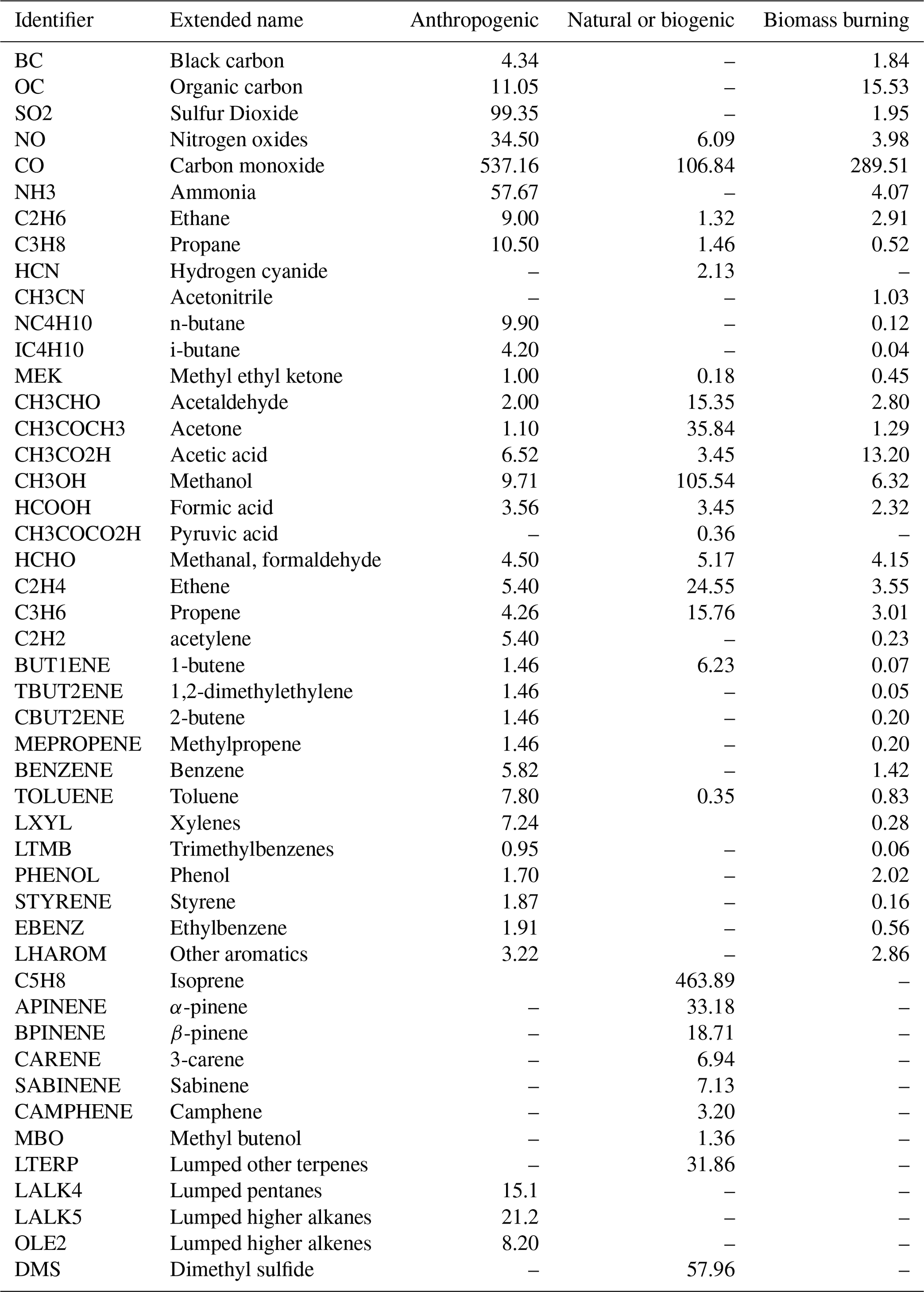
In Table 1 the total emissions are listed for all primary species emitted in the model.
Table 1Emissions of primary emitted species for the year 2010 used in this study. The values are given in units of Tg (species) yr−1 with the exception of NO, which is given in Tg (N) yr−1.
Dry deposition and sedimentation are estimated by the DDEP (Dry DEPosition) and SEDI (SEDImentation) submodels (Kerkweg et al., 2006a), while wet deposition is simulated by the SCAV (SCAVenging) submodel (Tost et al., 2006). The dissolution of species in the liquid-phase mechanism was augmented by including the liquid–gas equilibrium for all additional organics present in the mechanism with a Henry's law constant (solubility) above 103 . For less soluble species, wet scavenging is not expected to be important (Crutzen and Lawrence, 2000). The Henry's law constants of most oxygenated VOCs of atmospheric relevance are unknown, and estimation methods still quite uncertain (Wang et al., 2017). As the hydroxyl (and hydroperoxyl) group affects the solubility in water the most, the Henry's law constants of polyols from the compilation by Sander (2015) are taken as proxies.
In the chemistry submodel MECCA (Module Efficiently Calculating the Chemistry of the Atmosphere), we used the Mainz Organic Mechanism (MOM, Sander et al., 2019), with roughly 600 species and 1600 reactions. It originates from a reduced isoprene oxidation mechanism (Taraborrelli et al., 2009), which has been updated with recent kinetic data and expanded with efficient mechanisms of OH-recycling under low-NO conditions (Taraborrelli et al., 2012; Nölscher et al., 2014). The oxidation mechanism for α-pinene and β-pinene is based on the MCM (Master Chemical Mechanism, Jenkin et al., 2000) with modifications according to theoretical work in the literature (Vereecken et al., 2007; Capouet et al., 2008; Nguyen et al., 2009; Vereecken and Peeters, 2012). The degradation of monocyclic aromatics follows the MCM (Jenkin et al., 2003; Bloss et al., 2005) but with some modifications for the chemistry of phenols (Cabrera-Perez et al., 2016). The complete mechanism used in this study is part of the Supplement.
Aerosol microphysics and gas–aerosol partitioning are calculated by the Global Modal-aerosol eXtension (GMXe) aerosol module (described by Pringle et al., 2010a, b). GMXe simulates the distribution of aerosol within interacting lognormal modes (in a similar approach to that of Vignati et al., 2004; Mann et al., 2010). The lognormal modes span four size categories (nucleation (<6 nm radius), Aitken (6–60 nm), accumulation (60–600 nm) and coarse (>700 nm)) and are divided into hydrophilic (4) and a hydrophobic (3) modes. The GMXe model has been extensively evaluated previously (Pozzer et al., 2012a, b; Tost and Pringle, 2012; Karydis et al., 2016).
Organic aerosol (OA) formation is simulated by the submodel ORACLE (Tsimpidi et al., 2014, v.1.0), where logarithmically spaced saturation concentration bins are used to describe the organic aerosol components based on their volatility. For the formation of primary (POA) and secondary (SOA) organic aerosol from the emissions and photochemical oxidation of semivolatile and intermediate volatility organic compounds, the setup of Tsimpidi et al. (2016) is used. However, the SOA formation from the oxidation of the volatile organic compounds (VOC) in ORACLE has been modified to accommodate the photochemical production of components explicitly calculated by the MOM chemical mechanism. An earlier version of MOM has been compared against chamber measurements (Nölscher et al., 2014) and improved by Novelli et al. (2020), while ORACLE was derived empirically from chamber experiments (Donahue et al., 2011) and has been evaluated against observations from a field campaign by Janssen et al. (2017). Nevertheless, the MOM + ORACLE combination still has to be fully evaluated.
The effective saturation concentration of all the species present in the MECCA submodel is calculated based on their elemental composition (number of carbon, oxygen, nitrogen and sulfur atoms), following the molecular corridor approach (Li et al., 2016) and the study by Donahue et al. (2011). In Fig. 1, the volatility versus the molar mass is shown for all tracers present in the model, ranging from high volatility–low molar mass to low volatility–high molar mass. These calculations result in 199 tracers that can partition to the aerosol-phase, forming SOA under atmospheric conditions (i.e. with a volatility lower than 3.2×10³ µg m−3), while the other 396 tracers are considered too volatile for any condensation on aerosol particles. Additionally, the enthalpy of vaporization for the same condensing species has been estimated based on the study by Epstein et al. (2010). In addition to the 199 tracers, 11 additional “lumped species” for different oxidation levels of pentanes, higher alkanes, higher alkenes and terpenes have been added. Following this, ORACLE calculates the partitioning of these organic species between the gas and particle phases by assuming a bulk equilibrium and by further assuming that all organic compounds form a pseudo-ideal solution. The aerosol size distribution is determined by distributing the change in aerosol mass after the bulk equilibrium into each size mode using a weighting factor (Tsimpidi et al., 2014).
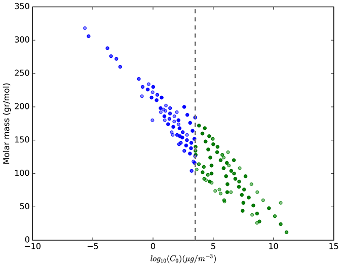
Figure 1Saturation mass concentrations at 298 K (Li et al., 2016) versus molar mass of organic tracers in EMAC. The blue dots represent those included in ORACLE, i.e. organic tracers that are allowed to condense explicitly on aerosols under atmospheric conditions; the green dots represent those organic tracers that are always in the gas phase. The dashed line represents the maximum volatility considered in ORACLE (i.e. 3.2×10³ µg m−3) for the VOC oxidation products.
The aerosol optical properties are calculated with the submodel AEROPT (Dietmüller et al., 2016), which is based on the scheme by Lauer et al. (2007) and makes use of predefined lognormal modes (i.e. the mode width σ and the mode mean radius have to be taken into account). Lookup tables with the extinction coefficient, the single-scattering albedo, and the asymmetry factor for the shortwave part of the spectrum and the extinction coefficient for the longwave part of the spectrum are pre-calculated with the help of Mie theory-based explicit radiative transfer calculations (see Pozzer et al., 2012a; Dietmüller et al., 2016). The aerosol compounds explicitly considered for their refractive indices are organic carbon, black carbon, dust, sea salt, water-soluble compounds (WASO, i.e. all other water soluble inorganic ions, e.g. , , , ) and aerosol water (H2O).
3.1 Aircraft measurements
Due to the high complexity of the MOM mechanism, we do not expect the model to be capable of representing polluted episodic conditions. Additionally, investigations of these conditions should be accompanied with detailed process studies, as has been done in previous studies with this mechanism (e.g. Lelieveld et al., 2018; Tadic et al., 2021). Instead we want to demonstrate its ability to reproduce background conditions in a climatological sense. For this reason, three different aircraft databases were chosen, which are all based on profiles of several flights and seasons, are taken over background regions, and provide an extensive set of observed trace gases.
3.1.1 NASA ATom campaign
We used observational data from the NASA Atmospheric Tomography Mission (ATom). The ATom campaign took place from July 2016 to May 2018 and included measurements in four different seasons (six flights each). During the flights with the NASA DC-8 aircraft, numerous profiles were recorded (see Fig. 2), which makes the dataset perfect for the evaluation of atmospheric model simulations. The data used in this evaluation was taken from the “Merged Atmospheric Chemistry, Trace Gases, and Aerosols, Version 2 dataset” (Wofsy et al., 2021) and are based on the following instruments: the UC-Irvine Whole Air Sampler (WAS; Barletta et al., 2019), the Trace Organic Gas Analyzer (TOGA; Apel et al., 2021), the California Institute of Technology Chemical Ionization Mass Spectrometer (CIT-CIMS; Allen et al., 2019), the NOAA Chemical Ionization Mass Spectrometer (NOAACIMS; Veres et al., 2021), the Georgia Tech Ionization Mass Spectrometer (GTCIMS; Huey et al., 2019), the NOAA Nitrogen Oxides and Ozone Instrument (NOyO3; Ryerson et al., 2019), and the NOAA Picarro G2401 spectrometer (NOAA-Picarro; McKain and Sweeney, 2021). The ATom observations were subdivided into data for different regions for this study (Fig. 2; namely Northwest Pacific, Southwest Pacific, East Pacific, Southern Ocean, South Atlantic, North Atlantic, and North Canada/Alaska/Greenland) based on expected homogeneous properties of organic compounds in those regions. A climatological comparison between the simulated year (2010) and the data from the ATom campaign (2016–2018) will be performed in order to further evaluate whether the MOM mechanism is able to reproduce remote conditions. For that purpose we divided the altitude range into 12 bins (linearly between 0.5 and 12.5 km) and defined a maximum of 336 (7 regions × 4 seasons × 12 altitude bins) points of interest (POI). For each POI we compared the mean value of all observations in the specific region, altitude bin and season to the mean value of all accordingly simulated values in 2010 in the range of ±1 d around the flights conducted in that region.
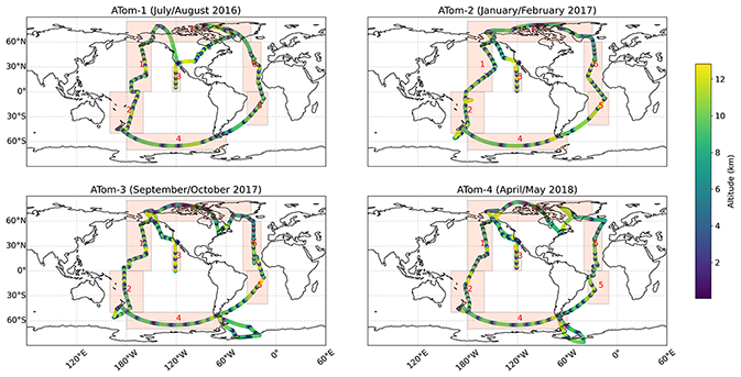
Figure 2Flight paths of the four ATom campaigns. The respective altitude is coloured, and the paths are sub-divided into seven different remote regions, namely the Northwest Pacific (1), Southwest Pacific (2), East Pacific (3), Southern Ocean (4), South Atlantic (5), North Atlantic (6), and North Canada/Alaska/Greenland (7).
3.1.2 Emmons database
We also used the database of aircraft measurements of trace gases produced by Emmons et al. (2000). It is based on observations from numerous aircraft campaigns that took place during the period 1990–2001 to create observation-based climatologies of chemical species relevant to tropospheric chemistry. Although these measurements cover only limited time periods and regions, they provide valuable information about the vertical distribution of the analysed trace gases. Note that the field campaigns used in this evaluation have been extended to also include observations after the year 2000, such as those from the TOPSE and TRACE-P campaigns.
3.1.3 Heald database
The aircraft evaluation is completed by aircraft measurements for organic aerosols presented by Heald et al. (2011). This dataset includes organic aerosol measurements from 17 aircraft campaigns during the period 2001–2009. Here, similar to Emmons et al. (2000), we consider the aircraft campaigns representative for the period and the regions, i.e. as an observation-based climatology. Therefore, we compared these data with the model results for the year 2010, yielding an improved evaluation of the vertical distribution of the organic aerosols in the troposphere.
3.2 Station measurements
3.2.1 NOAA-INSTAAR
Data from the National Oceanic and Atmospheric Administration (NOAA) Institute of Arctic and Alpine Research (INSTAAR) Global Monitoring Program were also used in this study. The network consists of 44 background stations from the NOAA Global Greenhouse Gases Reference Network (GGGRN) (Pollmann et al., 2008), where pairs of whole air samples are collected weekly and shipped to a central laboratory for analyses. For this study, we considered measurements of ethane, propane, iso-butane and n-butane from this network.
3.2.2 EPA
The Clean Air Markets Division of the U.S. Environmental Protection Agency (EPA) operates the Clean Air Status and Trends Network (CASTNET), with a total of 97 stations. Here, we include weekly filter pack data from 81 stations for , , , Na+, Mg2+, Ca2+, K+ and Cl− for the year 2010. The data can be downloaded at https://www.epa.gov/castnet (last access: 2 March 2022).
3.2.3 IMPROVE
In order to evaluate the simulated regional background OA concentrations, we use monthly averaged PM2.5 OA measurements during the year 2010 from the Interagency Monitoring of Protected Visual Environments (IMPROVE) program (http://views.cira.colostate.edu/fed, last access: 21 September 2021). IMPROVE is a cooperative measurement effort in the United States designed to characterize current visibility and aerosol conditions in scenic areas (primarily national parks and forests). This network includes 198 monitoring sites that are representative of the regional haze conditions over North America. IMPROVE co-located samplers collect 24 h samples every 3 d.
3.2.4 EMEP
The co-operative programme for monitoring and evaluation of the long-range transmission of air pollutants in Europe (EMEP) is a science-based and policy-driven programme under the Convention on Long-range Transboundary Air Pollution for international co-operation to solve transboundary air pollution problems. We use data from 42 stations, although the number of stations providing sufficient data for a certain species ranges from 22 to 42 (see Table 6). As Teflon filters are predominantly used, depending on the respective station, the concentrations of particulate nitrate can be systematically underestimated (Ames and Malm, 2001). The data were obtained from the EBAS database (http://ebas.nilu.no/, last access: 21 September 2021), and stations that did not provide full coverage of monthly mean values for the year 2010 were excluded from the analysis.
3.2.5 EANET
The Acid Deposition Monitoring Network in East Asia (EANET) regularly has monitored acid deposition since January 2001. A total of 13 countries currently participate in this effort, submitting data from a total of 54 sites. We use monthly averaged aerosol concentrations from 15 to 25 stations for the year 2010, with the data obtained from the Network Center for EANET, which are archived at https://monitoring.eanet.asia/document/public/index (last access: 2 March 2022). It is worth mentioning that EANET does not include OA observations. The simulated PM2.5 OA over East Asia is evaluated against collected short-term measurement data as summarized by Jo et al. (2013).
3.3 Remote sensing observations
3.3.1 MOPITT
MOPITT (Measurement of Pollution in the Troposphere) is a sensor onboard the NASA's Terra satellite. We use the MOPO3JM version 8 product of MOPITT, which provides monthly mean gridded column-integrated CO, vertical profiles of CO mixing ratios at 10 regularly spaced pressure levels from the surface up to 100 hPa and the corresponding averaging kernels (Deeter et al., 2019). The MOPO3JM product is based on the joint near-infrared (NIR) and thermal-infrared (TIR) retrievals of CO. We apply the MOPITT averaging kernels to the EMAC CO profiles according to Eq. (1) to ensure the same level of smoothing as that in the MOPO3JM product.
Here, xtrue is the EMAC profile, xa is the a priori profile, A is the averaging kernel matrix and I represents an identity matrix.
3.3.2 MODIS
The MODerate resolution Imaging Spectroradiometer (MODIS) sensor is also located on the Terra satellite. Here, AOD550 data (i.e. aerosol optical depth at 550 nm) from the MODIS Level 3 (Col. 6.11) gridded product are used at a spatial resolution of . The data are available through the Atmosphere Archive & Distribution System (LAADS) (https://ladsweb.modaps.eosdis.nasa.gov/, last access: 21 September 2021). The Deep Blue algorithm (Hsu et al., 2004) was used here for the aerosol AOD.
3.3.3 IASI
Global observations of a suite of VOCs are retrieved from the thermal infrared measurements of the nadir-viewing IASI (Infrared Atmospheric Sounding Interferometer) instruments (Clerbaux et al., 2009). The VOC dataset exploited here consists of total column densities of methanol, acetone, formic and acetic acids, and PAN, all retrieved on a near-global and daily basis from the IASI/MetOp-A observations with the aid of the ANNI (Artificial Neural Network for IASI) v3 retrieval framework. This neural-network-based retrieval approach does not rely on a priori information of the total column densities, and hence the products can be used directly for unbiased comparisons with model data (see Franco et al., 2018; Whitburn et al., 2016). The satellite products are filtered for measurements affected by clouds and poor retrieval performance. The uncertainties on the individual retrieved column densities can be large but are considerably reduced by averaging numerous observations in space and time, as has been done in this study by comparing annual averages on the model grid. A full description of the ANNI framework, the characterization of the VOC products, and comparisons of the satellite data with independent measurements can be found in Franco et al. (2018, 2019, 2020), Mahieu et al. (2021) and references therein. These studies, thanks to comparisons with ground-based column density measurements of VOCs and column densities derived from aircraft profiles, indicate no large systematic biases in the IASI data and no dependence on the latitude, although an underestimation (locally up to 30 %) of the highest column densities over tropical source regions (e.g. the Amazon basin) has been identified for all the IASI VOC products (except PAN). The accuracy of the IASI measurements is therefore sufficient to provide a global evaluation of the EMAC performance, considering the large uncertainties that still affect the emissions and atmospheric modelling of the VOCs. For both IASI and the model, daily gridded averages were constructed at the spatial resolution of the model grid. To have similar temporal coverage over the year between model and satellite observations, the EMAC daily averages were masked when the corresponding IASI data were missing for the same day and location.
3.3.4 AERONET
The AOD observations have been obtained from the global AErosol RObotic NETwork (AERONET Holben et al., 1998; Dubovik et al., 2000). The cloud-screened quality-assured Level 2 AOD data used in this study were obtained from the website http://aeronet.gsfc.nasa.gov/cgi-bin/combined_data_access_new (last access: 21 September 2021), including the AOD daily averages.
3.4 Pseudo-observations
Global annual averages of fine particulate matter with an aerodynamic diameter below 2.5 µm (PM2.5) have been obtained from Hammer et al. (2020). In this dataset, a combination of satellite-observed AOD, numerical model and ground-based PM2.5 measurements were used to estimate PM2.5 on a global scale at high resolution.
In Table 2 the evaluation of organic tracers using observations from the ATom campaign is presented, while Table 3 shows the comparison of the model results with the aircraft campaign data from Emmons et al. (2000) for selected tracers. There are no measurements of acetic acid (CH3COOH) from the ATom campaign, and the observations of ethene (C2H4) and propene (C3H6) are very limited. Thus, they will not be considered for discussion. In the Emmons database, there are no observations of i-butane (i-C4H10) and n-butane (n-C4H10).
Table 2Summary of simulated and observed mixing ratios of different tracers from the ATom campaign (Wofsy et al., 2021). N.points is the number of points used for the statistical estimation. The arithmetic mean of the model simulated mixing ratios (), the observed mixing ratios () and the corresponding standard deviations (MSTD, OSTD) (in pmol mol−1) are listed in the subsequent columns (for CO and O3 units are nmol mol−1). PF2 denotes the percentage of simulated points within a factor of 2 with respect to the observations, and RMSE represents the root-mean-square error between simulated and observed points. CORR is the Pearson correlation coefficient.
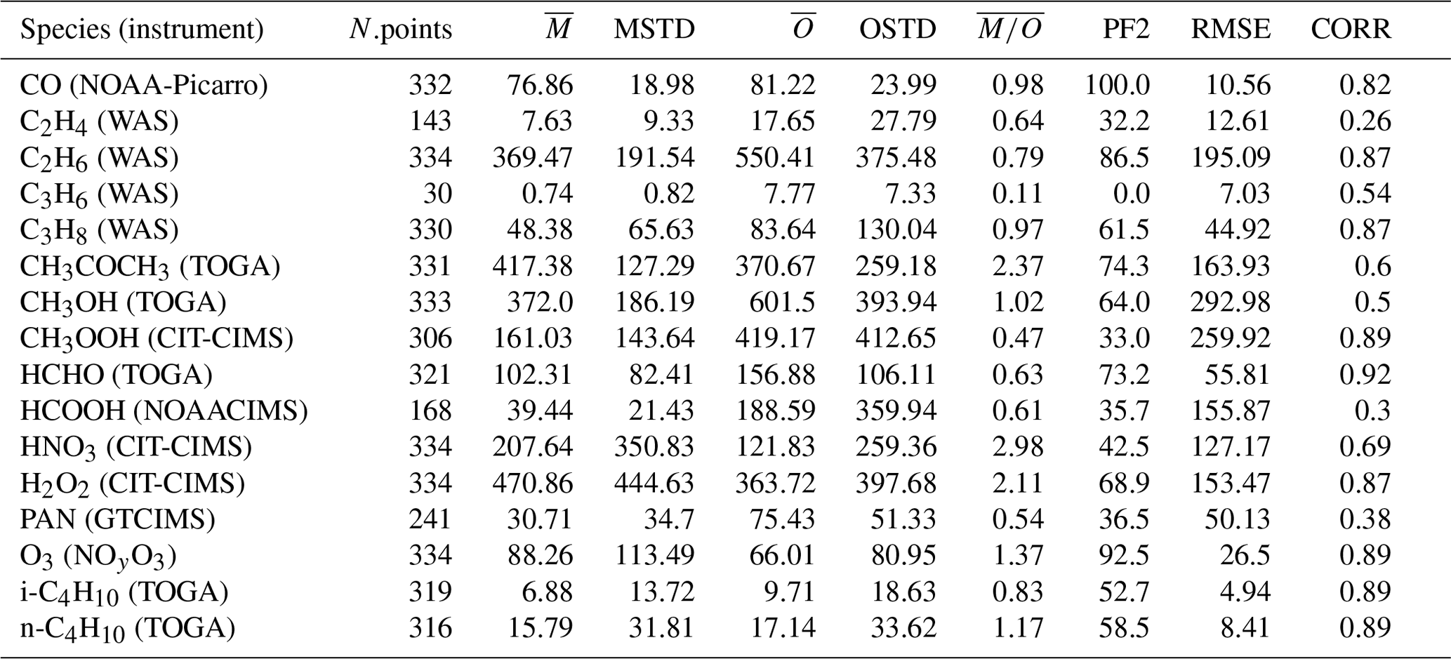
Table 3The same as Table 2 but for the comparison of our simulation results to the dataset of Emmons et al. (2000).
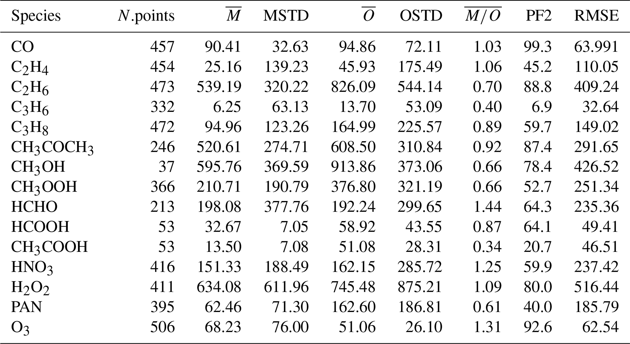

Figure 3Scattered simulated values of CH3OOH and HCHO against the observations of the ATom measurements. The different colours represent the altitude. Both species are generally underestimated by our simulations, but at the same time there is a high correlation between the simulation and observations.
CO, C2H6 and O3 are very well represented because more than 85 % of the simulated values are within a factor of 2 compared to the observations for these species (PF2). Other species (such as PAN) show insufficient agreement with both observation sets, while other species do not show consistent behaviour between the comparisons. For some species (such as the alkene C3H6 in the Emmons database), a general clear underestimation is seen in the Emmons database, which is coherent with previous results (Pozzer et al., 2006). An interesting feature can be observed for methyl hydroperoxide (CH3OOH) and formaldehyde (HCHO): both species are strongly underestimated by the simulation compared to the ATom observations (see Table 2; of 0.47 and 0.61, respectively), while they are highly correlated with the observations (≈0.9). Thus, the vertical shape is very well reproduced, but the sources and sinks seem to be systematically underestimated and overestimated, respectively. This feature is depicted in Fig. 3. The evaluation results for selected species will be analysed in more detail in the following.
4.1 CO
Figure 4 shows the seasonal (MAM: March, April, May; JJA: June, July, August; SON: September, October, November; DJF: December, January and February) mean modified EMAC and MOPITT CO vertical column densities (VCDs). Here, we term it as “modified” EMAC VCDs because MOPITT averaging kernels are applied to the simulated CO profiles to account for the sensitivity of MOPITT. To highlight the difference in spatial patterns of EMAC and MOPITT, we also show the absolute bias in the bottom panel.
We note that the spatial patterns are in good agreement between simulation and observations. In particular, the elevated CO background in the outflow regions (over oceans) in the northern hemisphere is well represented during boreal winter (DJF) and spring (MAM). The outflow region around South America in SON is also simulated well. Over land, a good agreement is found for Europe, the central and eastern United States, northern Africa, Australia, Russia, and the Indian subcontinent, with a mean bias within . During the biomass burning seasons (JJA in central Africa and north and northeast China and SON in South America), we observe an overestimation of ∼ 30 % by EMAC. By comparing EMAC's total CO column densities to IASI CO satellite retrievals, Rosanka et al. (2021a) found that EMAC underestimates CO in Indonesia in SON 2015. In 2015, a particularly strong El Niño led to severe peatland fires, which resulted in large CO emissions. Rosanka et al. (2021a) attribute the underestimation to a too low biomass burning emission factor for peatland used by EMAC. Here, we do not find any underestimation of CO in Indonesia in SON (see Fig. 4), as the year 2010 was a year with low biomass burning emissions in Indonesia (van der Werf et al., 2017). Following their analysis, the recent biomass burning emission factor estimate by Andreae (2019) suggests that EMAC underestimates the CO emission factor by about 10 % in central South America and Africa. It must however be stressed that the uncertainties in the biomass burning emissions are substantial, depending on regions and species (Carter et al., 2020). In contrast, in South America the overprediction of EMAC's CO column densities can be partially attributed to EMAC's tendency to overestimate biogenic emissions of CO precursors in this region (see Rosanka et al., 2021b, a), as also shown in Sect. 4.2.3 and 4.2.4.
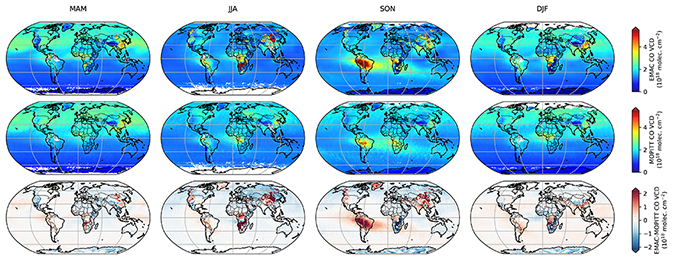
Figure 4Global seasonal mean maps of CO vertical column densities (VCDs) for the year 2010 for EMAC (top), MOPITT (middle) and bias (EMAC − MOPITT) (bottom).
Figure 5 shows the 2010 annual mean measured and simulated surface CO mixing ratio at the WDCGG stations sorted according to their latitude coordinates. The relative bias at all stations is also shown on a global map in the inset of Fig. 5. Similar latitudinal gradients are seen for the measurements and simulations with high values around the mid-latitudes of the Northern Hemisphere. The measured and simulated CO agree within 1σ annual variability for 106 out of 113 stations for which data were available for the year 2010. The bias between model and simulation was found to be less than 20 % of the observations for 96 stations.

Figure 5Latitudinal gradient of the annual mean (2010) of the measured and simulated surface CO mixing ratio at the WDCGG measurement stations. The error bars show the 1σ standard deviation of the annual mean (based on daily mean output). The map in the inset shows the annual bias between the simulation and measurements at the locations of the WDCGG stations.
4.2 Volatile organic compounds
4.2.1 C2–C4 alkanes
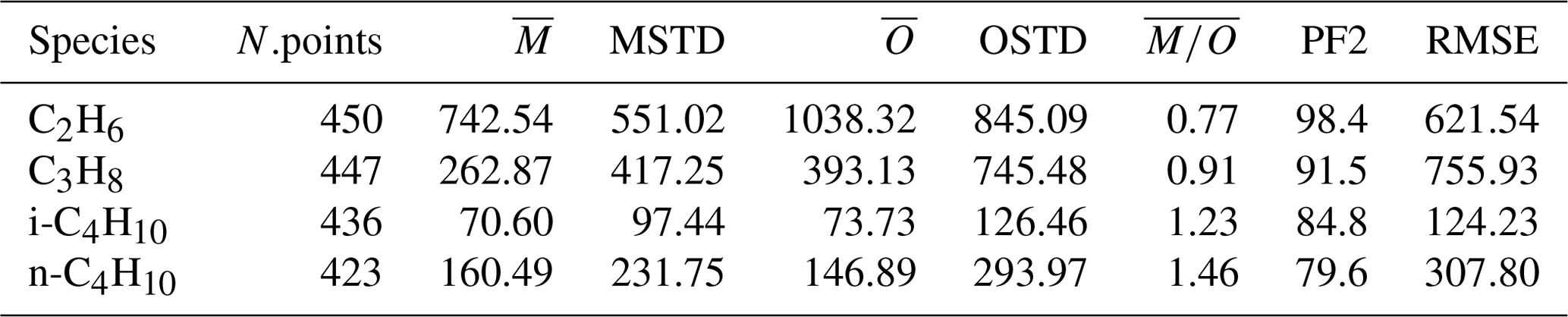
Alkanes are VOC ubiquitously present in the atmosphere that are mainly emitted from anthropogenic activities. In Fig. 6 the scatterplots of model results and in-situ observations from the NOAA/INSTAR database are presented. The statistic for each plot is summarized in Table 4. The model seems to reproduce satisfactorily the mixing ratios of the C2–C4 alkanes with more than 98 %, 91 %, 84 % and 79 % of the simulated values lying within a factor of 2 of the observations for C2H6, C3H8, i-C4H10 and n-C4H10, respectively. Furthermore, the average ratios show that a slight overestimation is present for i-butane and n-butane, whereas the model underestimates the mixing ratios of ethane and propane. This is confirmed by the comparison with the Emmons et al. (2000) database (Table 3), which shows that both ethane and propane are underestimated by the model with respect to the vertical profile as well (column ). The comparison with ATom observations (Table 2) also shows an underestimation (albeit smaller) of ethane and propane. However, for i-butane we see a slight underestimation in the evaluation using ATom observations in contrast to the NOAA/INSTAR database.
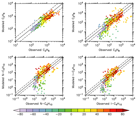
Figure 6Scatterplot of measured and simulated surface alkanes mixing ratios at the NOAA/INSTAAR measurement stations for the year 2010 (in pmol mol−1). The colour code denotes the latitude of the stations.
Figure 6 also shows a noticeable underestimation of the mixing ratios in the region between 30 and 0∘ N for propane and the butanes. This is clearly due to the underestimation of the oceanic emissions, as these stations (i.e. at Mahe Island, Seychelles (SEY); The American Samoa Observatory (SMO); Ascension Island, UK (ASC); and Easter Island, Chile (EIC)) are all strongly influenced by oceanic emissions. It must be pointed out that no oceanic emissions were included in the simulation for i-C4H10 and n-C4H10 but that these are necessary for a correct representation of butanes, as already shown previously (Pozzer et al., 2010). However, the underestimation in this region is not present in the comparison to the ATom observations.
Table 4Summary of simulated and observed mixing ratios of different tracers in the NOAA/INSTAAR database (station observations). The columns are the same as in Table 3.
4.2.2 C2–C3 alkenes
In contrast to alkanes, the alkenes are mostly emitted by the biosphere. The comparison to the ATom campaign can only be based on a very limited number of observations, and thus it will not be covered in this discussion. As shown in Table 3 in the comparisons with the Emmons et al. (2000) database, the numerical simulation of alkenes diverges more from the observations than the simulated alkanes do. Both C2H4 and C3H6 are underestimated compared to the observations (see the model mean against observed mean comparison in Table 3). Nevertheless, while C2H4 is reasonably reproduced overall (the average of the ratios is equal to 1.06; see Table 3), for C3H6 a strong underestimation is present (the average of the ratios is equal to 0.4; see Table 3). This is shown in Fig. 7, where examples of the vertical distribution of C2H4 are shown. The issues in simulating C3H6 have been already pointed out by Pozzer et al. (2006), where similar results were obtained with large underestimation of this tracer. As alkenes are mostly removed by reaction with OH, there are strong indications that these reactions are too fast; in addition, a substantial lack of emissions could be present, for instance from natural sources, as suggested by Li et al. (2021).
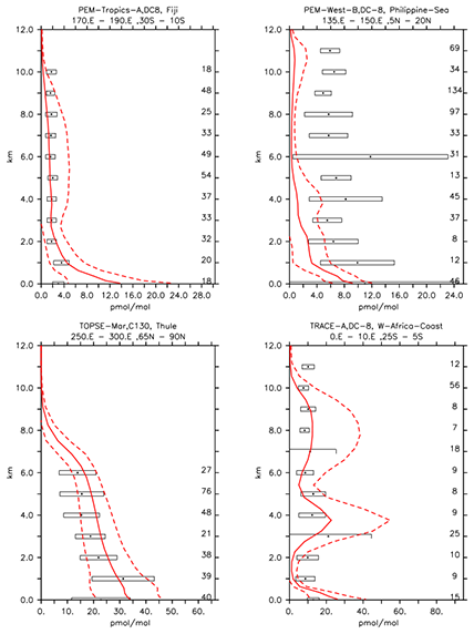
Figure 7Vertical profiles of C2H4 (in pmol mol−1) for some selected campaigns from Emmons et al. (2000). Asterisks and boxes represent the average and the standard deviation (with respect to space and time) of the measurements in the region, respectively. The simulated average is indicated by the red line, and the corresponding simulated standard deviation with respect to time and space is indicated by the dashed lines. The number of measurements is listed on the right-hand side.
4.2.3 CH3OH
CH3OH is the most abundant oxygenated VOC in the Earth's atmosphere (Singh et al., 2001) and is primarily emitted by terrestrial vegetation (Jacob et al., 2005). Other sources include biomass burning, the oceans and secondary formation in the troposphere (see, e.g. Millet et al., 2008; Stavrakou et al., 2011). The annual global distributions of CH3OH total column densities obtained from the IASI measurements and EMAC of the year 2010, as well as their differences, are presented in Fig. 8. Over land, the satellite and model spatial distributions of CH3OH are relatively consistent, with the main source regions observed within the tropics (mainly over the Amazon basin and central Africa), in Southeast Asia, and at Northern Hemisphere mid-latitudes and high latitudes. However, important differences in magnitude exist. Over tropical forests, EMAC indeed simulates annual CH3OH column densities up to 2 times larger than those retrieved from the IASI observations (3.0–3.5 × 10¹⁶ ). This can be partly ascribed to the high temperature bias that exists in the model over these areas (Hagemann and Stacke, 2015), which induces an excess of biogenic VOC emissions from the MEGAN submodel due to its high temperature sensitivity (Guenther et al., 2006). This is confirmed by a comparison of the simulated isoprene mixing ratios in the Amazon rainforest with observations from the AMAZE-08 campaign (Martin et al., 2016) and from the ATTO tower (Yáñez Serrano et al., 2015). In comparison to the AMAZE-08 campaign, the simulated isoprene measurements are overestimated by more than a factor of 3 (6.1±1.2 nmol mol−1 simulated and 1.9±1.4 nmol mol−1 observed), while the overestimation factor for the ATTO tower is on average approximately 1.6, being higher in February–March and lower in October–November.
Furthermore, dry deposition of methanol in tropical rainforests is likely under-represented by the Wesely (1989) approach used here (Karl et al., 2004). The potential contribution of an additional non-stomatal pathway favourable under humid conditions (Müller et al., 2018) has been shown by Emmerichs et al. (2021) for a less soluble species. On the other hand, EMAC underestimates the CH3OH column densities at mid-latitudes and high latitudes of the Northern Hemisphere, indicating that biogenic and/or biomass burning VOC emissions are too low during summertime in these regions. The southeastern US is the region in North America where most of the simulated CH3OH enhancement exists, driven by substantial biogenic emissions in summertime, while larger column densities are measured by IASI during the same season further northwards in the boreal regions. Over the oceans, EMAC underestimates the observed CH3OH column densities by ∼5 × 10¹⁵ , which might result from an insufficient transport from the continental source regions and/or from missing secondary source(s) (see, e.g. Bates et al., 2021; Müller et al., 2016). This is confirmed by the comparison of model results with the aircraft observations of the ATom campaign and the Emmons et al. (2000) database, where the methanol model mean is considerably lower than the observed one. This is most prominent over Pacific regions in the Northern Hemisphere at lower altitudes, as depicted in Fig. 9. However, with respect to the vertical profile CH3OH is not generally underestimated in comparison with the ATom campaign, as it is instead overestimated at higher altitudes and for lower absolute values.
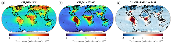
Figure 8Annually averaged CH3OH total column densities (in ) from IASI satellite observations (a) and simulated by EMAC (b) and the EMAC-to-IASI column density differences (c) for the year 2010.

Figure 9Vertical profiles of CH3OH of model simulations and ATom observations over the Pacific region (region 1 in Fig. 2) in the Northern Hemisphere, represented by box and whisker plots for altitude bins. The white line marks the median, the box corresponds to lower and upper quartiles, and the whiskers represent the 5th and 95th percentiles. The numbers on the right indicate the number of points of interest (POI, averaged values for region, flight and altitude) considered for each altitude bin.
4.2.4 CH3COCH3
Acetone is the one of the most abundant oxygenated VOCs in the Earth's atmosphere after CH3OH (Singh et al., 2001). Its sources include the terrestrial vegetation, the oxidation of hydrocarbon precursors of biogenic and anthropogenic origin, the oceans, and biomass burning (e.g. Jacob et al., 2002; Pozzer et al., 2010; Fischer et al., 2012). The acetone column densities obtained from the EMAC simulation and the IASI observations exhibit major discrepancies in terms of global distribution (Fig. 11). The satellite instrument detects the largest acetone column densities (up to 2 × 10¹⁶ ) at mid-latitudes and high latitudes of the boreal hemisphere, ascribed to important emissions of biogenic precursors during summertime (Franco et al., 2019), but a moderate burden at low latitudes and over the tropical forests. It is worth noting that this pattern is in agreement with the global acetone measurements obtained with the ACE-FTS satellite limb sounder (Dufour et al., 2016). Conversely, EMAC simulates strong hotspots of acetone within the tropics, especially over South America and Africa, with annually averaged column densities larger than 2 × 10¹⁶ , but underestimates the acetone abundance by up to a factor of 2 in the Northern Hemisphere. Such a mismatch between satellite and model distributions points to major deficiencies in the current emission inventories of acetone and its precursors. For example, the extremely large acetone column densities simulated by EMAC over the Persian Gulf and the Indo-Gangetic Plain can be attributed to the highly elevated emissions of propane – an important precursor of acetone – in these regions. In vegetated regions, an underestimation of acetone dry deposition, accounting for 20 % of the total loss globally (Khan et al., 2015), likely contributes to the mismatch. According to measurements, significant amounts of acetone are removed during the night through non-stomatal uptake (Karl et al., 2004; Müller et al., 2018). However, over remote areas and the oceans, the simulated acetone abundance is consistent with the IASI measurements, with vertical column densities in the range of 0.5–1.0 × 10¹⁶ . The model nevertheless simulates a slight overestimation over the oceans at low latitudes compared to IASI, especially in the outflows of the tropical hotspots.
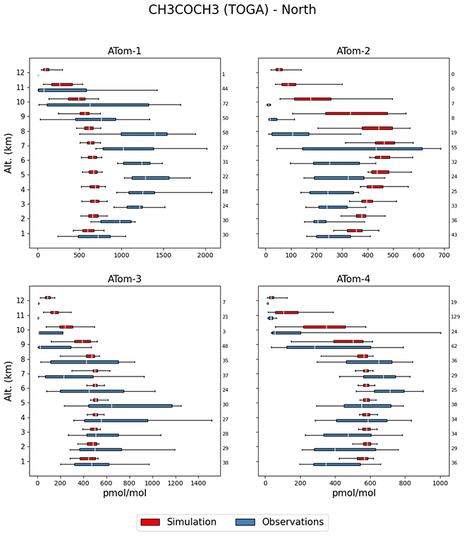
Compared to the ATom observations the model overestimates the mixing ratios, especially at high altitudes, leading to a large value of , while the simulated and observed mean are of a comparable magnitude. However, 74.3 % of the simulated values are still within a factor of 2 of the observations (see Table 2). Figure 10 depicts the vertical column densities of observations and simulations over the northern part of North America and Greenland, a region where CH3COCH3 is largely underestimated by the model in comparison to IASI. In Northern Hemisphere summer (July–August; ATom-1) this strong underestimation can also be observed for the ATom observations. However, for other seasons this is not the case. Overall, simulation results show only a small underestimation for this region. Compared to the Emmons et al. (2000) database, the model results present a much better agreement, with only a somewhat small bias (see Table 3). This apparent agreement with the observations is due to the uneven distribution of the field campaign present in the observational dataset (see Emmons et al., 2000, their Fig. 1, and Huijnen et al. (2019), their Fig. 1). In fact, most of the campaigns in which acetone was measured took place over the ocean, where the model is correct or slightly overestimates the total column densities observed by IASI. In contrast, only few campaigns in the Northern Hemisphere are present in the dataset (such as ABLE-3B and POLINAT-2) for which the model strongly underestimates the observed values. As a result of the sparsity of these observations, Table 3 presents a quite fair agreement between model and aircraft observations, an agreement which is, however, not corroborated by the more spatially complete comparison with the IASI total column densities.

Figure 11The same as Fig. 8 but for CH3COCH3.
4.2.5 HCOOH
Formic acid is the dominant organic acid in the troposphere and a product of the degradation of a large suite of VOC precursors, but its observed abundance is generally severely underestimated by state-of-the-art global models (e.g. Millet et al., 2015; Paulot et al., 2011; Stavrakou et al., 2012). Similarly, in our simulation the EMAC model largely underestimates the HCOOH total column densities derived from the IASI observations by up to a factor of 4, particularly in remote environments (see Fig. 12). Although the two main tropical source regions identified by IASI – the Amazon basin and central Africa – are reproduced by EMAC, the magnitudes of the simulated HCOOH column densities are too low in comparison to the satellite measurements. It also has to be mentioned that the apparent agreement over Amazonia is possibly due to the high temperature bias in the region and the subsequent excess of simulated isoprene emissions during the dry season. Over the other source regions (e.g. Southeast Asia and the southeastern US), the model underestimation is more pronounced, particularly in the Northern Hemisphere. The large enhancement of HCOOH column densities observed with IASI over western Russia ( ), attributed to the August 2010 wildfires, is not reproduced by EMAC ( ) and suggests that the biomass burning emissions of VOCs are underestimated.
The general underestimation of simulated versus observational data is also confirmed by the comparison with aircraft observations. The model strongly underestimates the observations by the ATom campaign, especially at low altitudes and for high absolute values (see Table 2, the observed mean is higher by more than a factor of 4 compared to the model mean). In general, there is very low agreement between simulated values and ATom observations, as only around 35 % of the simulated values are within a factor of 2 of the observations and the Pearson correlation coefficient is only 0.3. Although the underestimation of the model results compared to the Emmons et al. (2000) database is less apparent, it must be noted that only a limited number of merged data (53; see Table 3) is available for the comparison with aircraft observations. It must be stressed that Franco et al. (2021) showed the importance of in-cloud chemistry for this tracer, which is missing in this study. The lack of adequate in-cloud chemistry would therefore explain the almost ubiquitous underestimation of this tracer.
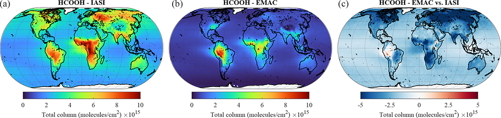
Figure 12The same as Fig. 8 but for HCOOH.
4.2.6 CH3COOH
Acetic acid is the second most abundant carboxylic acid in the troposphere and, based on the IASI retrievals, presents a spatial pattern, regional seasonality and vertical abundance that resemble those of HCOOH (Franco et al., 2020). Like the latter, CH3COOH is produced from the oxidation of various tropospheric precursors but has emission factors from biomass burning that are 3 to 10 times larger than those of HCOOH (Akagi et al., 2011; Andreae, 2019). CH3COOH is more difficult to detect in the infrared IASI spectra, and its retrievals are subject to larger uncertainties, particularly over ocean (see Franco et al., 2020). Therefore, here we limit the comparison with EMAC to the continents, excluding measurements over desert areas that are altered by surface emissivity artefacts (Fig. 13). From the comparison, conclusions similar to those of HCOOH can be drawn for CH3COOH: the two main tropical source regions are relatively well reproduced by EMAC (with a better agreement over Africa in this case), whereas the observed CH3COOH levels are underpredicted in the Northern Hemisphere by up to a factor of 4. The comparison with aircraft observations (see Table 3) again confirms this strong underestimation over the ocean as well, as the only campaign in the dataset including CH3COOH measurements is the PEM-Tropics-A, which was performed over the Pacific ocean.
These results confirm that the VOC emissions and oxidation pathways leading to the formation of CH3COOH in the troposphere are still poorly understood and constrained (e.g. Khan et al., 2018; Paulot et al., 2011). For example, acetaldehyde – a major CH3COOH precursor via its reaction with OH (Lei et al., 2018) – is well known to be largely underestimated by global models (Millet et al., 2010; Wang et al., 2019). On the other hand, the large model versus observations differences in Southeast Asia also point to missing emissions from biomass burning. Finally, in-cloud chemistry could be important in the CH3COOH formation, analogous to formic acid (Franco et al., 2021), and this process could bring model results and observations to a closer agreement.
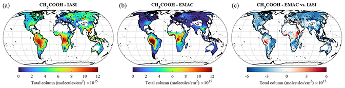
Figure 13The same as Fig. 8 but for CH3COOH. Note that areas above ocean have been excluded.
4.2.7 PAN
Owing to its complex photochemical sources and its thermal instability, PAN (peroxyacetyl nitrate), the main tropospheric reservoir species of NOx, is a very challenging tracer to simulate. The comparison with the IASI data reveals that the model correctly reproduces the main spatial patterns of PAN, with the source regions and main outflows over the oceans being correct. However, the model constantly underestimates the observed PAN column densities over the globe. The satellite column densities are indeed between 2 and 4 times the simulated ones, with the most pronounced negative bias observed at Northern Hemisphere mid-latitudes and high latitudes. The same conclusion can be drawn from the comparison with aircraft observations (Tables 2 and 3), for which the model clearly underestimates the observed mixing ratios consistently using the database from Emmons et al. (2000) and the measurements of the ATom campaign. A closer inspection reveals that PAN is especially underestimated in the middle and upper troposphere. The model–observation discrepancies can mostly be attributed to the unsatisfactory representation of different VOCs. For example, we have seen that the model results do not agree with observations for acetone, which is an important precursor of the peroxyacetyl radical in the free troposphere (Fischer et al., 2014). Furthermore, the strongest model underestimation appears to be exactly where CH3COCH3 the most underestimated, confirming that deficiencies in simulated precursor patterns are the main cause of the PAN biases. Additionally, sensitivity simulations suggested that the PAN formation in global models is more sensitive to the representation of VOCs than the one of NOx (Fischer et al., 2014). Finally, an insufficient vertical transport of VOCs from the planetary boundary layer to the free troposphere in the model might also reduce the amount of PAN because PAN is more stable at the lower temperatures of the free troposphere.

Figure 14The same as Fig. 8 but for PAN.
4.3 OH
The simulated distribution of the hydroxyl radical (OH) is in line with the findings by Lelieveld et al. (2016) (further denoted as L16), who earlier thoroughly analysed the MOM performance in EMAC with a setup featuring a simplified treatment of aerosol microphysics and gas–aerosol partitioning. The total OH turnover (composition of annual production and loss terms, shown in Fig. 15) of 234 Tmol yr−1 in 2010 is 7 % less than that found by L16 and is consistent with the addition of the explicit treatment of secondary organic formation processes of aerosols and changes in trace gas emission fluxes. The OH production in the VOC- and ROOH-initiated reactions is 3 % lower in both the free troposphere (FT) and the boundary layer (BL). This is compensated for by the increased share of primary production (P, via the O(1D) + H2O pathway), especially in the BL (4 % increase versus 2 % in the FT). Regarding the partitioning of the OH sinks, however, no substantial changes can be noted (see Fig. 15b and d). Together with the reduction of the secondary sources (S), the resulting OH recycling probability rOH (defined as ; see details in L16) is established at 59 % and 62 % in the BL and FT, respectively. Being about 5 % lower than the estimate reckoned by L16, such high rOH values still signify highly stable (buffered) OH concentrations and therefore a likewise stable tropospheric oxidative capacity obtained with this model setup.
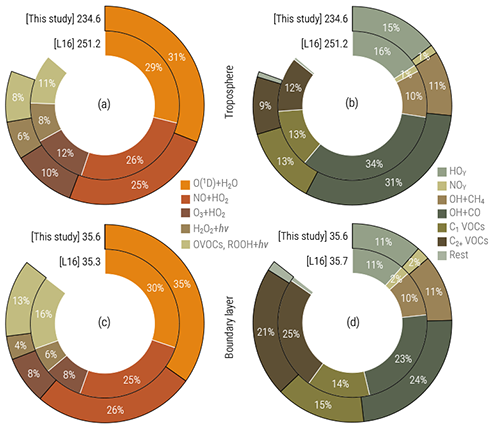
Figure 15Simulated OH production (a, c) and sink (b, d) by category in the troposphere (a, b) and boundary layer (c, d) in this study and the study of Lelieveld et al. (2016) (denoted L16). Values are annual totals (in Tmol yr−1) for 2010. Percentages denote fractions attributed to particular categories (see L16 for details).
The simulated annual air-mass-weighted average OH concentrations are 12.1 (troposphere), 12.0 (FT) and 13.6 (BL) 105 for the year 2010, which correspond to OH chemical removal lifetimes of 1.59, 1.78 and 0.53 s, respectively. The diagnosed tropospheric OH inter-hemispheric gradient (Northern Hemisphere to Southern Hemisphere ratio, NH / SH) is 1.17, lower than that estimated by L16 (1.20) due to the increased OH reactivity via VOC and SOA in the NH and at the lower end of the model estimates reviewed there. By not being in agreement with the measurement-based estimates suggesting hemispheric symmetry in tropospheric OH (Patra et al., 2014; Wolfe et al., 2019), the pronounced asymmetry in atmospheric models results from asymmetric OH production due to skewed distributions of O3 and NOx prevailing in the NH and calls for further studies in this direction.
Overall, the simulated tropospheric OH distribution is comparable to that which was thoroughly analysed by L16 with a minor increase in reactivity of up to 5 % when calculated from the changes to the CH4 and MCF (CH3CCl3) lifetimes against removal by OH (τOH). The τOH (CH4) values estimated here are 8.4 and 4.4 years in the FT and BL, respectively; the tropospheric τOH (MCF) value is determined to be 4.9 years.
4.4 Aerosol optical depth
In order to evaluate the overall performance of the model in reproducing aerosol distribution, the AOD at 550 nm simulated by the model is compared to satellite-based and station observations. Figure 16 shows the annual average AOD of the simulation and of the observations (satellite). The distribution is remarkably similar, with the high AOD regions (northern Africa and Southeast Asia) being well simulated by the model. Open-ocean AOD of ≃0.2 AOD units are reproduced by the model, with slightly underestimated AOD over the central Atlantic (possibly due to slightly underestimated dust outflow from the northern Africa region). To quantify the model capability to reproduce the AOD, in Fig. 17 the model daily AODs are compared to the co-located (in space and time) observations from MODIS and the AERONET instruments (middle and bottom row, respectively). For comparison, the same scatterplot has been produced comparing MODIS and AERONET directly (top row). The model has difficulties in reproducing the daily variability of AERONET AOD, with only 58 % of the simulated AOD within a factor of 2 of the observational data. Even the correlation is considerably low, with an R2 equal to 0.33. Very similar results are obtained by comparing the model results to the satellite AOD observations, with again only 57 % of the simulated data within a factor of 2 of the observations. Once monthly averages are used for the inter-comparison, the statistics remain almost unchanged with just a small improvement in the slope of the fitting curve (see Fig. 17, central column). Finally, using the annual averages for the intercomparison, the coefficients of determination R2 almost double (0.633 and 0.567 for the comparison of the model with MODIS and AERONET data, respectively), while more than 80 % of the model results are within a factor of 2 of the observations (either satellite or in situ). To put these results into context, the same analysis has been performed comparing the MODIS data and AERONET stations. Although the satellite observations (slightly) outperform the model results compared to the AERONET-measured AOD in the case of the daily and monthly averages, for the annual averages the model seems to perform equally well, with a similar coefficient of determination and a fraction of values within a factor of 2 of the observations. Due to the intrinsic characteristics of the model (such as its relatively coarse resolution) it is not expected to have a good representation of the short-term variability.
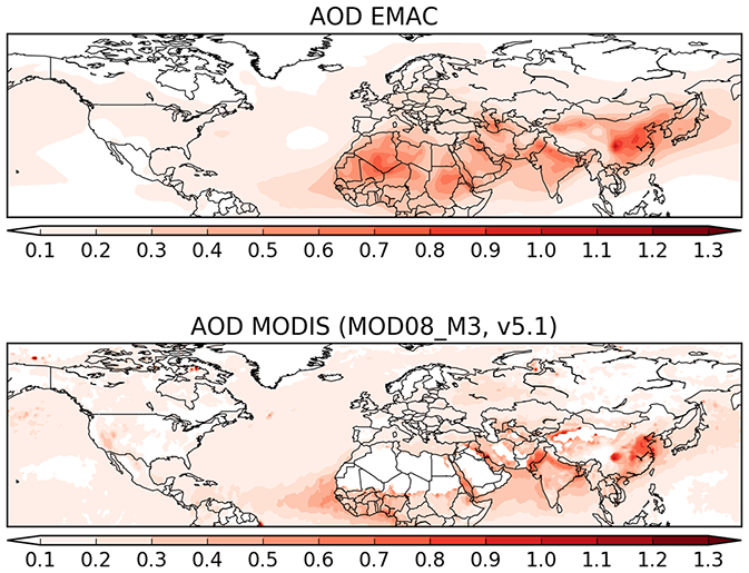
Figure 16Global map of AOD from model results and the MODIS observations for the year 2010 (annual average).
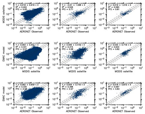
Figure 17Scatterplots of AOD estimated by the EMAC model in this study versus the MODIS and the AERONET observations. The left, middle and right columns show scatterplots using daily, monthly and annual averages, respectively. Both model- and satellite-based observations were sampled at the AERONET locations. In each plot the coefficients of the linear fit, the coefficient of determination and the fraction of data within a factor of 2 are listed.
4.5 Fine particulate matter (PM2.5)
The comparison of model results for PM2.5 (i.e. fine particles with an aerodynamic diameter smaller than 2.5 µm) was performed against the dataset of Hammer et al. (2020). Although this dataset is not a pure observational dataset, it has a global coverage and has been constrained from in situ measurements. The comparison is done for PM2.5 at 35 % relative humidity, i.e. dry fine particulate mass (in µg m−3). In Fig. 18, the maps of the annual average of the model results and the pseudo-observation dataset are shown. Although the distribution patterns appear to be similar, the model underestimates the fine particle concentration over northern India and eastern China, whereas the opposite happens over eastern Africa and the Middle East. On the other hand, the model seems to reproduce PM2.5 quite accurately over both Europe and North America, and even the locally enhanced levels of PM2.5 (∼30 µg m−3) in Canada from boreal forest biomass burning are reproduced well by the model.
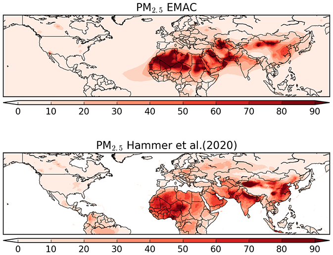
Figure 18Global map of PM2.5 from model results and the Hammer et al. (2020) dataset for the year 2010 (annual average, in µg m−3). The data from Hammer et al. (2020) does not contain values over the ocean.
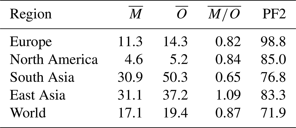
In Fig. 19, the scatterplot of the two datasets is shown, while in Table 5 the statistics for the different regions presented in the figures are listed. Due to the large grid resolution difference, the pseudo-observations have been aggregated to the grid resolution of the model. As already noted from the global map, the model underestimates PM2.5 over South Asia and East Asia by ∼40 % and ∼20 %, respectively. Nevertheless, in both regions more than 70 % of the model results are within a factor of 2 of the pseudo-observations. As shown by Pozzer et al. (2012a, 2017) and more recently by Miao et al. (2020), BC and OC are very important for the PM2.5 budget in East Asia and South Asia. As shown by Crippa et al. (2018) and Saikawa et al. (2017) the emissions of these tracers are associated with large uncertainties in these regions, which could strongly affect our results. However, the model agrees well with data from Europe and North America, with more than 95 % of the model results being within a factor of 2. The overall comparison indicates that the model agrees well with the pseudo-observations, as the spatiotemporal averages of the two datasets are very close (17.1 µg m−3 for the model and 19.4 µg m−3 for the pseudo-observations), with more than 70 % of the model-simulated PM2.5 within a factor of 2 of the pseudo-observed PM2.5.
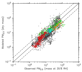
Figure 19Scatterplots of PM2.5 of model results versus data from Hammer et al. (2020) for the year 2010 (annual average, in µg m−3). Light blue, red, green and orange depict points located in Europe, North America, East Asia and South Asia, respectively. Grey points indicate the remaining parts of the world.
Table 5Summary for simulated and pseudo-observed annually averaged PM2.5. and denote the arithmetic mean of the simulated and observed concentrations, respectively (in µg m−3). PF2 is the percentage of simulated points within a factor of 2 with respect to the observations.
4.6 Aerosol composition
For the evaluation of the simulated mass concentrations of sulfate, nitrate, ammonium, sodium, and five species related to sea spray and organic aerosols, we use in situ measurements from different monitoring networks, as described in Sect. 3.2. Co-located time series of simulated and observed quantities were obtained via bilinear interpolation of the gridded model data at ground level to the respective site location. The analysis is based on monthly mean concentrations, which are derived from daily (model data, EMEP observations) and weekly (EPA) data, with the exception of EANET, which directly provides monthly averages. Note that some monitoring stations are located relatively close to each other, such that the reported concentrations may not be independent of each other, which can lead to an overestimation of the degrees of freedom in the calculation of quantities such as the root-mean-square error.
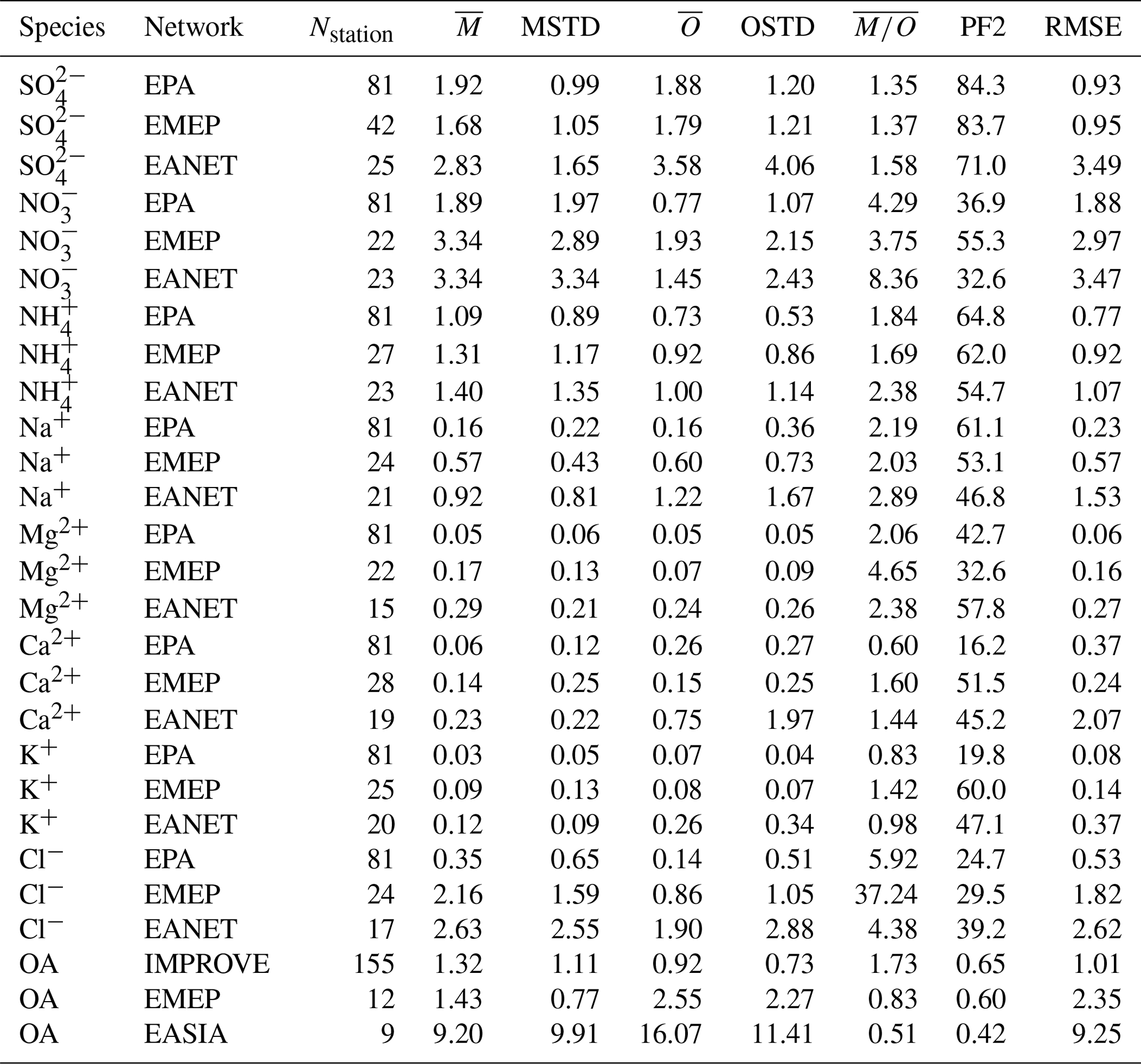
Table 6Summary of simulated and observed monthly averaged aerosol concentrations for , , , Na+, Mg2+, Ca2+, K+, Cl− and organic aerosols (OA) and different observational networks (second column). Nstation is the number of stations providing data for the respective species and network; note that this is not the sample size for the shown statistics. The following columns provide the arithmetic mean of the simulated () and observed concentrations () and the respective standard deviations (MSTD, OSTD, in µg m−3). PF2 denotes the percentage of simulated points within a factor of 2 with respect to the observations, and RMSE represents the root-mean-square error between simulated and observed points.
4.6.1 Sulfate ()
Observed particulate sulfate concentrations are reproduced well by the model. The monthly mean concentration is matched closely for North America (EPA) and slightly underestimated for Europe (EMEP) and East Asia (EANET) (see Table 6). For EPA and EMEP data, more than 80 % of the simulated monthly mean concentrations lie within a factor of 2 of the observations, as do more than 70 % of the concentrations for EANET. The standard deviation of observed monthly mean values is lower than the root-mean-square error (RMSE) for all monitoring networks, which is an indication for a good quality of the model results (Barna and Lamb, 2000). In addition, RMSE is lower in the present study compared to a similar analysis by Pozzer et al. (2012a) in which a longer time period of 4 years (2005–2008) was investigated. Pozzer et al. (2012a) also report a relatively large spread (observation standard deviation equal to 5.3 µg m−3) of the measured sulfate concentrations in EANET, which is likely caused by a comparably low number of stations that cover a large region with strong spatial gradients.
The close overall agreement of average concentrations simulated by the model () with the observations () for EPA can partly be attributed to underestimated high concentrations in summer (composite of June, July and August, JJA), which are compensated by overestimated lower concentrations from autumn to spring (see Fig. 20). Relative deviations are largest in winter and autumn, when observed concentrations are much lower than simulated concentrations. In Europe (EMEP), the highest concentrations are observed during the winter months, which is captured by the model.
The east–west gradient of observed annual mean concentrations in North America is represented well in the model, although the amplitude is underestimated by the model: lower observed values in the west are overestimated, while higher observed concentrations in the east are underestimated by the model (Fig. 21). This feature also led to a good agreement between observed and simulated mean concentrations in Table 6. The north–south gradient over Europe is also captured by the model. Despite the less dense spatial distribution of monitoring stations providing data for particulate sulfate, one can observe a correspondence between simulated and observed annual mean concentrations, especially over Japan. One outlier in Japan with a very low observed annual mean concentration is located at a relatively high altitude (Happo, 1850 m), and thus the comparison to model data on ground level may not be appropriate for this station. The same holds for two EMEP stations, namely Jungfraujoch (Switzerland) at 3578 m, and Chopok (Slovakia) at 2008 m, where annual mean concentrations are largely overestimated, possibly due to the coarse resolution of the model, which cannot correctly reproduce the orography (and hence the altitude) of these stations. We therefore compared concentrations with observations from aircraft campaigns, as compiled by Heald et al. (2011). The results are presented in Fig. 22. The simulated sulfate concentrations agree well with the aircraft observations in the free and lower troposphere, with an underestimation in a few cases (see Fig. 22; during the ITCT-2K4, ADIENT or IMPEX campaigns) but always within the measured standard deviations, confirming that the vertical profile of sulfate is generally well reproduced in the lower troposphere.
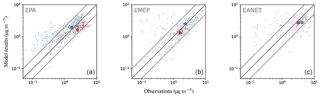
Figure 20Scatterplots of observed and simulated monthly average concentrations for the year 2010 and three observational networks: EPA, EMEP and EANET (a–c). The colouring of the points represents a categorization into seasons (dark blue: DJF; orange: MAM; red: JJA; light blue: SON); the seasonal averages of monthly concentrations are depicted as large circles. Dashed lines denote the interval of a factor of 2 of the observations. The simulated concentrations were obtained by sampling the modelled data at the respective station locations using bilinear interpolation over neighbouring grid points.

Figure 21Annual mean concentrations for the year 2010 for the model and three observational networks: EPA, EMEP and EANET (a–c). Simulated data are shown as shaded contours, while the observational data are depicted as circles.

Figure 22Model results of mean vertical profile of sulfate aerosol for selected field campaigns in black, and the spatiotemporal standard deviation is shown as a grey area. The observed mean values are depicted in solid red, with the bars representing the standard deviation of the observations. The observed median is presented as dashed red line.
4.6.2 Nitrate ()
Nitrate is less well represented than sulfate, showing a general overestimation of observed concentrations with an average ratio of simulated to observed concentrations of at least 3.75. This comparably large ratio is dominated by a few stations with small concentrations, where the median ratios lie between 1.70 and 2.84. About half (EMEP) to two-thirds (EPA, EANET) of the simulated monthly mean concentrations exceed a factor of 2 with respect to the observations. For EANET and EMEP, the number of monitoring stations is substantially lower than for EPA, which may partly explain the larger spread in both the model results and observations (OSTD, MSTD). The RMSE is larger than the observed standard deviations for all considered networks, suggesting a less faithful representation of this species. This overestimation may be attributed to the usage of Teflon filters, as nitrate can evaporate from the filters under warm and dry conditions (Ames and Malm, 2001). Schaap et al. (2004) and de Meij et al. (2006) showed that particulate ammonium and nitrate partially evaporate from the filters at temperatures between 15 to 20 ∘C and can evaporate completely at temperatures above 20 ∘C. Therefore, this effect predominantly affects measurements during the warmer seasons when nitrate concentrations are close to the annual minimum. An indication for overestimation due to evaporation would then be a closer agreement between model and observation in the colder winter months. However, both in relative and absolute terms, the overestimation of monthly mean nitrate concentrations is more pronounced in winter than in summer for the three considered networks (Fig. 23). All regions show the same seasonal cycle with respect to averaged monthly mean concentrations: a maximum in winter and a minimum in summer both for model results and observations. The spatial gradient of the annual mean concentrations is captured well for North America (EPA), although the concentrations towards the east coast are generally overestimated. The low number of monitoring stations for EANET and EMEP does not allow us to draw solid conclusions; however, we can report that the north–south gradient of nitrate over Europe is reproduced by the model, with the exception of an outlier at high altitude in Central Europe (Fig. 24). The region with the highest simulated annual mean concentrations and strongest spatial gradients is East Asia; however, it is sparsely covered by monitoring stations reporting full coverage for the considered year 2010.
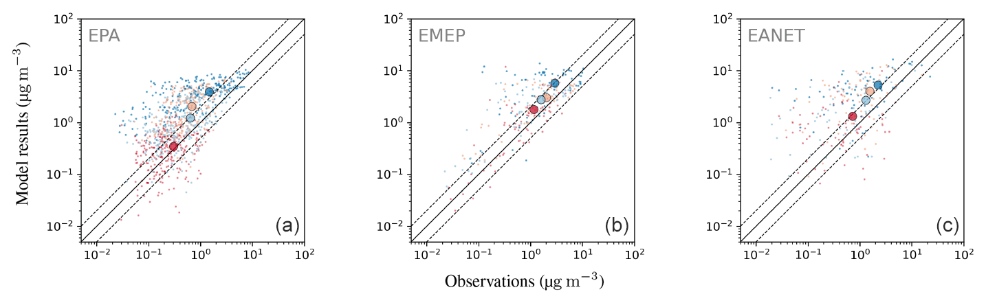

Figure 24The same as Fig. 21 but for .
4.6.3 Ammonium ()
Considering the ratio of averaged monthly mean ammonium concentrations, the model overestimates the observed concentrations but to a lower degree than for nitrate (Table 6). This feature is also apparent in the fraction of simulated monthly mean values within a factor of 2 of the observations: 54.7 % for the network in East Asia and more than 60 % for Europe and North America. The magnitude of overestimation is similar for the three networks, ranging from 40 % to 50 %. RMSE values are close to the standard deviation of observations in all networks, again indicating a good representation by the model. The largest concentrations occur during the winter months (Fig. 25). While the degree of overestimation is similar for the different seasons in EMEP and EANET, this does not hold for EPA: summer concentrations are systematically underestimated, whereas autumn to spring concentrations are generally overestimated. The concentrations for winter and spring constitute most of the values that are outside the aforementioned factor of 2 threshold regarding the observations for all considered regions. Both the observed north–south and east–west gradients of annual mean concentrations are represented well for the EPA network (Fig. 26), but the simulated gradient is less pronounced.
The north–south gradient of observations over Europe is also captured by the model, although the number of stations is again comparably low. The simulated spatial patterns in East Asia also arguably match the observations well.
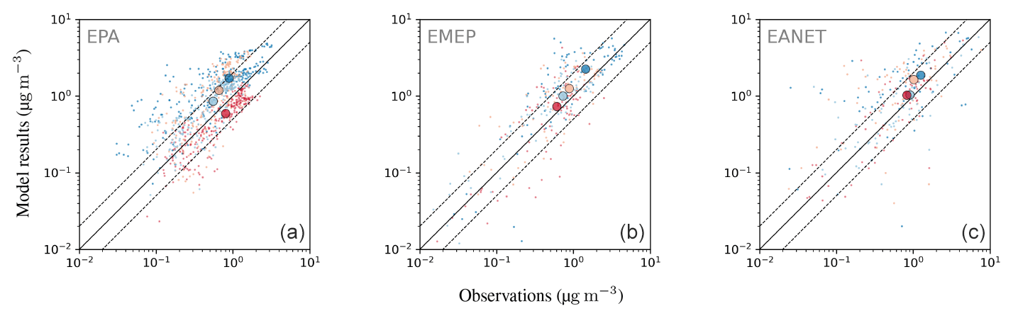
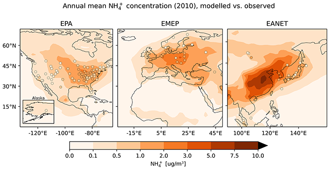
Figure 26The same as Fig. 21 but for .
4.6.4 Dust and sea spray
This section provides an overview for species frequently found in dust and sea spray aerosol: sodium, calcium, magnesium, potassium and chloride. As the ocean is a large source of these water-soluble species, concentrations over the sea and coastal areas are large, as opposed to lower concentrations over the continents. Sodium, potassium, magnesium and calcium can also be found in desert dust, for instance in the Sahara, as reported by Reid et al. (2003) and Moreno et al. (2006). However, most of the monitoring locations except for those in coastal areas are sampling quite remote sites far from the source regions, and thus they cannot be expected to display the full range of concentrations. In the following section, we present the results for sodium in more detail, followed by a brief overview of the remaining species.
Sodium is represented well by the model, as averaged monthly mean concentrations from model and observations agree in general, particularly for EPA (Table 6). The mean ratio , however, shows an average overestimation by a factor of at least 2. The observational standard deviation (OSTD) for all regions is smaller than the RMSE, the latter being reduced compared to the results from a previous study by Pozzer et al. (2012a). For EMEP, more than three out of five simulated monthly mean values lie within a factor of 2 of the observations and more than 53 % and 46 % for EMEP and EANET, respectively, which is a substantial improvement compared to Pozzer et al. (2012a). The latter two networks again offer only a small number of stations. Considering the average of monthly mean concentrations separated by season, one can observe an underestimation of summer concentrations for all networks (Fig. 27).
As mentioned before, the regional distribution of stations does not cover those regions with high concentrations. However, when including the information of all networks at once, one can observe that continental stations exhibit low annual mean concentrations, while high concentrations can for instance be observed at stations close to the coast (i.e. Japan, Florida, Denmark, Sweden), indicating that spatial features of the global sodium distribution are qualitatively captured (Fig. 28).
Potassium, magnesium and calcium ions share spatial features with sodium in the model, exhibiting elevated values over the ocean, as well as over the Sahara and Gobi desert, and reduced concentrations over other continental areas.
The number of stations in EANET is quite low for all sea spray species, which, on the one hand, allows for a few outliers to dominate mean values and errors. On the other hand, EPA offers a large number of stations, yet the correspondence between model and observations is also quite low for sea spray and dust species. Average monthly mean concentrations for magnesium are represented well in the model, which is caused by a large overestimation of concentrations in winter months balancing an underestimation of summer concentrations (not shown).
Chloride concentrations are widely overestimated with respect to all three networks. The exceptionally high ratio for EMEP is caused by two outliers with due to very low observed concentrations. Without these factors, is better, with a value of 13.08.

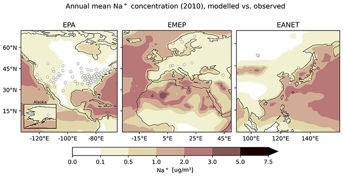
Figure 28The same as Fig. 21 but for Na+.
4.6.5 Organic aerosols (OA)
Figure 30 shows the comparison of model-calculated OA concentrations with measurements from the EMEP observational network over Europe, the IMPROVE network over rural North American locations, and short-term measurement data collected over East Asia as summarized by Jo et al. (2013). As we only used measurements taken in the year 2010, a low number of observations are present for East Asia, and the comparison must be taken cautiously for this region. The comparison statistics are presented in Table 6. The model captures the monthly average concentrations of OA relatively well over these highly populated regions of the Northern Hemisphere. This is rather encouraging given the expected uncertainties of the emission inventory and the complex chemistry involved in simulating the secondary organic aerosol formation. It is worth emphasizing that the model considers the formation of SOA solely from the homogeneous gas-phase photochemical oxidation of its precursors. Therefore, the omission of other SOA formation pathways (e.g. from aqueous-phase and heterogeneous reactions) can add to the model bias. This is mostly evident during winter (e.g. over Europe), when the relative importance of these processes on SOA formation increases due to the lower photochemical activity and the limited conversion of gas-phase organic precursors to SOA. In addition, recent studies have provided strong evidence that the uptake of water-soluble gas-phase oxidation products (even small carbonyls like formaldehyde and acetic acid) can be the main driver of SOA pollution during haze events over East Asia (Gkatzelis et al., 2021). Given the coarse resolution of the model and its inability to simulate these SOA formation pathways, the observed total OA concentrations are expected to be systematically underestimated by the model over East and South Asia. Nevertheless, model results are in general in reasonable agreement with observations, with the exception of the strong underestimation over Beijing and Shijiazhuang, which brings the to very low value (i.e. 0.51). As pointed out by Miao et al. (2021) and Zhao et al. (2016), the emission inventories for semivolatile and intermediate-volatility organic compounds are insufficient and lead to the majority of the model biases in simulating OA in these regions that are influenced significantly by anthropogenic emissions.
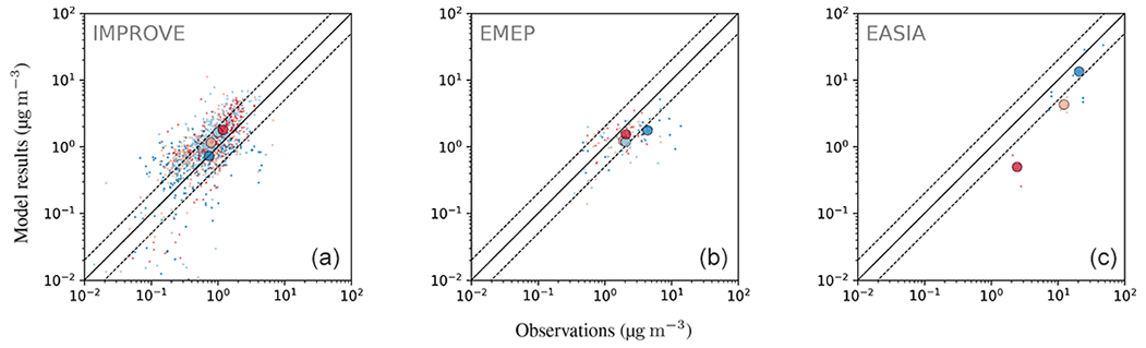
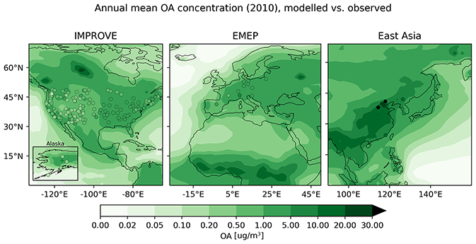
Figure 30The same as Fig. 21 but for OA.
Over Europe, the model also underestimates OA, with of 0.83 (see Table 6). The model performs worst during winter. Tsimpidi et al. (2016) have identified the lack of biomass burning emissions as the main source of this discrepancy over Europe. Kodros et al. (2020) and Paglione et al. (2020) have more recently shown evidence that biomass burning also contributes significantly to SOA formation during winter following its oxidation by the NO3 radical in the dark. Over North America, the model overestimates OA over rural areas, with a equal to 1.73. However, as shown in Fig. 29, part of this discrepancy is explained by the low values of OA over the US national parks.
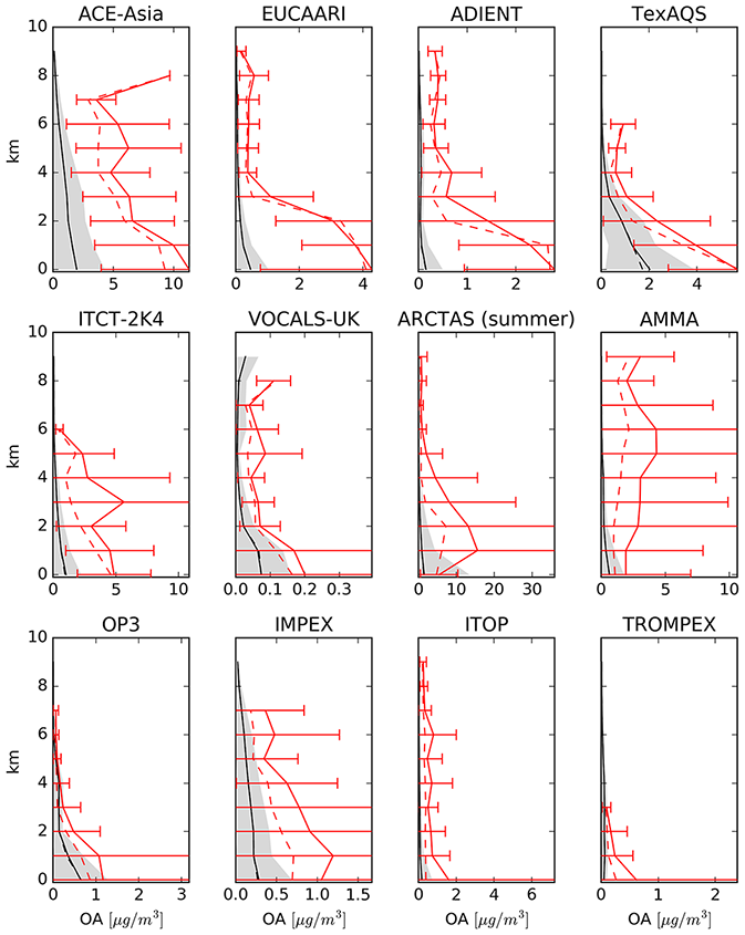
Despite the agreement of the surface OA concentrations between model results and observations, the OA are strongly underestimated in the free troposphere. In Fig. 31, the model is compared with 12 field campaign measurements (Heald et al., 2011). Our results show similar agreement to those obtained by Heald et al. (2011), with the simulated values being below the observed values.
We have presented an evaluation of EMAC with a comprehensive degradation scheme for organics (MOM) in the MECCA chemistry submodel combined with an explicit estimation of the organic tracers' condensation on aerosols with a VBS approach (ORACLE submodel). We have compared the model results with a large number of in situ and satellite-based remote sensing observations. The evaluation focuses on carbon monoxide (CO), simple organics and aerosols, which are the samples most influenced by the new scheme. CO is correctly reproduced compared with station measurements, with the correct north–south gradient. Nevertheless, once the model results are compared with the satellite observations from MOPITT, an overestimation of CO over the Amazon basin is apparent, especially in autumn, possibly due to an overestimation of the biomass burning emissions simulated by the model. For alkanes the comparison shows a good agreement, although an oceanic source for the butanes is missing. In contrast, the model underestimates alkenes, especially C3H6, which shows large differences compared to the observations. Model results of oxygenated species show an indifferent picture when compared to observations depending on the tracer: while methanol is well reproduced, simulated acetone shows large spatial discrepancies compared to the remotely sensed observations. For the latter, the model in fact misses strong emissions over the boreal forests, while it instead predicts too high total columns over tropical forests (i.e. Amazonia and central Africa). Formic and acetic acid show similar agreement to the observations, with the main tropical sources being well reproduced, albeit with a strong underestimation elsewhere.
The aerosols at the surface are reproduced well by the model with respect to both composition and total amount. The annually averaged simulated AODs show a very good agreement with the AERONET station observations, but they show some deficiencies in the representation of the short-term variability. The agreement of the fine particulate mass (PM2.5) near the surface is also quite good, with most of the simulated values within a factor of 2 of the observations. The evaluation of the aerosol chemical composition shows a high level of agreement for near-surface sulfate and more deviation for and nitrate, which are both overestimated by the model (especially the latter), even though the observations are characterized with a high level of uncertainty. The mechanically produced primary aerosol species (dust and sea salt) show a reasonable agreement with the observations with some substantial overestimation of the simulated chloride concentrations indicating an acid displacement process that is too weak over the continents.
Finally, the comparison of OA shows a good agreement with station observations, while the vertical distribution of the simulated values are largely underestimated when compared with aircraft measurements, which is analogous to other global atmospheric chemistry models of similar complexity, although significant improvement in this direction has recently been published (Pai et al., 2020).
The presented model evaluation is useful for identifying areas for further model improvements. A few possible directions are discussed below.
Emissions have always been a critical point for simulating tropospheric chemistry. It has already been shown in many studies that even anthropogenic emissions of alkanes need to be improved as they are severely underestimated in many inventories (e.g. Emmons et al., 2015; Tilmes et al., 2016), mostly due to erroneous speciation of the total VOC emissions (Dalsøren et al., 2018)
Residential wood burning and/or biofuel use (e.g. for heating) that often contribute significantly to both POA and SOA formation over urban areas are strongly underestimated in the emission inventories (Tsimpidi et al., 2016; Denier Van Der Gon et al., 2015). In addition, global models lack OA emissions from residential and commercial cooking activities that can be an important source of OA (Mohr et al., 2012; Sun et al., 2011; Ge et al., 2012; Hayes et al., 2013). Underestimation of cold-start vehicle emissions (Weilenmann et al., 2009) can also lead to significant underestimation of OA formation from the transport sector (e.g. during wintertime).
As seen in this study, the model results underestimate selected VOCs in boreal regions. The thawing of permafrost is potentially an additional emission source of organic compounds at high latitudes in the Northern Hemisphere (Li et al., 2020) that has not been considered yet. However, an estimate with global datasets is still missing. Furthermore, the emission of VOCs from biomass burning is likely strongly underestimated. In fact, overwintering fires in boreal forest (Scholten et al., 2021), which smoulder through the non-fire season, are normally not detected by satellite observations and are therefore missing in our used emissions dataset. Moreover, peat fires are not easily detected from space but are characterized by larger emission factors for many VOCs. They are important for simulating air composition during peat fires in Indonesia (Rosanka et al., 2021a) and likely critical for resolving the model biases at high latitudes, where most of peatland is located and could be further released by permafrost thawing. Ramo et al. (2021) also found that small undetected fires enhance the estimated amount of emitted carbon from biomass burning in sub-Saharan Africa by 31 %–101 %. Finally, soil temperature and soil wetness play an important role in the estimation of the online emissions of biogenic VOCs, and it is therefore important to have a correct simulation of the surface properties by the underlying climate model.
Furthermore, dry deposition is a relevant process also affecting VOCs in the lower troposphere (Khan et al., 2015). The inclusion of the additional uptake at the plant cuticle leads to a better representation (Karl et al., 2004; Müller et al., 2018; Emmerichs et al., 2021) and would likely reduce the overestimation of species like acetaldehyde in the tropics, as shown here. In the Amazon rainforest, the missing storage capacity of soil water leading to too high temperatures (Hagemann and Stacke, 2015) additionally causes an underestimation of dry deposition (Emmerichs et al., 2021), while temperature-dependent processes like VOC emissions are overestimated.
Another source of uncertainty is related to the scavenging efficiency of gas-phase OA precursors. The water solubility of these oxidized organic vapours is largely unknown and is typically considered uniform for all organic compounds in modelling studies even though they become increasingly more hydrophilic during their atmospheric lifetime (Hodzic et al., 2014; Tsimpidi et al., 2017).
The extension of MOM for the oxidation of additional VOCs has the potential to reduce the negative model biases for some oxygenated volatile organic compounds (OVOCs) and enhance the predicted OA levels. For instance, with an emission strength of more than 40 Tg yr−1, anthropogenic C5 and higher hydrocarbons can be a significant source of OVOCs like acetaldehyde and acetone (Pozzer et al., 2010). Further improvements are expected from an extended representation of the emission and oxidation of known biogenic VOCs with more than five carbon atoms. Moreover, the emissions of aromatic compounds from biogenic sources could be as large as 40 Tg yr−1 (Misztal et al., 2015). So far only small emissions of toluene are considered, and a more comprehensive representation of biogenic aromatics would likely lead to further improvements.
The formation of SOA in most models relies on the reaction of its gas-phase precursors with reactive atmospheric radicals (e.g. OH, O3, NO3), and their chemical ageing is usually considered by the further photo-oxidation of the semivolatile products solely in the gas phase. However, SOA is also subject to oxidation in the aqueous phase through superficial and bulk interactions with gas-phase oxidants (George and Abbatt, 2010). Therefore, fundamental processes of SOA formation in the aqueous phase (e.g. from isoprene epoxydiols (Nguyen et al., 2009) and glyoxal (Fu et al., 2008)) are typically missing from the conventionally used parameterizations. In addition, the uptake of small carbonyls (e.g. aldehydes and acids) to the aqueous phase and their subsequent oxidation and oligomerization has been recently linked to significant increases of SOA mass during pollution events (Gkatzelis et al., 2021).
Recently, MOM has been coupled to the detailed Jülich Aqueous-phase Mechanism of Organic Chemistry (JAMOC, Rosanka et al., 2021c) for cloud droplets. An explicit treatment of multiphase chemistry of OVOC has already been used for assessing the global role of clouds as a sink of ozone (Rosanka et al., 2021b). By comparing EMAC's prediction of total methanol columns to IASI satellite retrievals (comparable to Sect. 4.2.3 and Fig. 8), they find that EMAC's tendency to overestimate methanol is partially reduced by the additional cloud sink. This suggests that the missing representation of in-cloud OVOC chemistry introduces a significant bias in the present study, and therefore a more detailed multiphase chemistry should be included for future studies. Furthermore, JAMOC is limited to the oxidation of OVOCs containing up to four carbon atoms (Rosanka et al., 2021c), and an expansion to larger species (i.e. containing more than four carbon atoms) is thus desirable, in order to improve the representation of these OVOCs in EMAC when using MOM. Based on the results of Franco et al. (2021), more detailed in-cloud chemistry could improve the representation of acids (such as acetic and formic acid), which is clearly underestimated here, where cloud chemistry is important.
Finally, the MOM + ORACLE framework calculates the phase partitioning of organic compounds by assuming a bulk equilibrium without any kinetic limitation. However, the phase state of the organic aerosol can affect the mixing time of the condensed organic compounds within the aerosol. In general, equilibrium partitioning to the particle phase is a reasonable assumption if the aerosol is liquid; however, if the phase state is solid, non-equilibrium partitioning should be considered. Shiraiwa et al. (2017) suggests that kinetic limitations in the bulk may not significantly affect SOA partitioning in the boundary layer, justifying the use of equilibrium partitioning in this part of the atmosphere, but kinetic limitations should be implemented and investigated for the free and upper troposphere.
The Modular Earth Submodel System (MESSy) is continuously further developed and applied by a consortium of institutions. The usage of MESSy and access to the source code is licensed to all affiliates of institutions which are members of the MESSy Consortium. Institutions can become a member of the MESSy Consortium by signing the MESSy Memorandum of Understanding. More information can be found on the MESSy Consortium Website (http://www.messy-interface.org, last access: 2 March 2022). The code presented here has been based on MESSy version 2.54 and is available in the official release of version 2.55.
The supplement related to this article is available online at: https://doi.org/10.5194/gmd-15-2673-2022-supplement.
AP, AT and VlK planned the research. AP designed, coded, prepared the input files and performed the model simulation with the help of SE. AP, ViK, SG, SFR, BF, SR, TE, DT, VF, AT and MK wrote the manuscript. DT and RS developed MOM and integrated it into MECCA. SG implemented extended budgeting of species turnover. AT and VlK modified ORACLE to accommodate the organic tracers from the MOM chemical mechanism. MC, DG and JWK provided the emissions for the simulations. AP, SFR, ViK, AT, DA and MK contributed to the evaluation. AKS corrected the manuscript. PJ and HT contributed to model development of the system applied here. BF and LC developed the IASI VOC products and performed the comparisons with EMAC.
At least one of the co-authors is a member of the editorial board of Geoscientific Model Development. The peer-review process was guided by an independent editor, and the authors also have no other competing interests to declare.
Publisher's note: Copernicus Publications remains neutral with regard to jurisdictional claims in published maps and institutional affiliations.
IASI is a joint mission of EUMETSAT and the Centre National d'Etudes Spatiales (CNES, France). The IASI Level-1C data are distributed in near real time by EUMETSAT through the EUMETCast distribution system. The authors acknowledge the AERIS data infrastructure (https://www.aeris-data.fr/, last access: 21 September 2021) for providing access to the IASI Level-1C data and Level-2 temperature data. IASI activities are supported by the Belgian State Federal Office for Scientific, Technical and Cultural Affairs (Prodex arrangement IASI.FLOW). Lieven Clarisse is a research associate supported by the F.R.S. – FNRS. Holger Tost acknowledges funding from the Carl Zeiss Foundation. We are grateful to Colette Heald for providing the aircraft data and for her support and suggestions to improve the manuscript.
The article processing charges for this open-access publication were covered by the Max Planck Society.
This paper was edited by Christoph Knote and reviewed by three anonymous referees.
Akagi, S. K., Yokelson, R. J., Wiedinmyer, C., Alvarado, M. J., Reid, J. S., Karl, T., Crounse, J. D., and Wennberg, P. O.: Emission factors for open and domestic biomass burning for use in atmospheric models, Atmos. Chem. Phys., 11, 4039–4072, https://doi.org/10.5194/acp-11-4039-2011, 2011. a, b
Allen, H., Crounse, J., Kim, M., Teng, A., and Wennberg, P.: ATom: L2 In Situ Data from Caltech Chemical Ionization Mass Spectrometer (CIT-CIMS), ORNL DAAC [data set], https://doi.org/10.3334/ORNLDAAC/1713, 2019. a
Ames, R. B. and Malm, W. C.: Comparison of sulfate and nitrate particle mass concentrations measured by IMPROVE and the CDN, Atmos. Environ., 35, 905–916, https://doi.org/10.1016/S1352-2310(00)00369-1, 2001. a, b
Andreae, M. O.: Emission of trace gases and aerosols from biomass burning – an updated assessment, Atmos. Chem. Phys., 19, 8523–8546, https://doi.org/10.5194/acp-19-8523-2019, 2019. a, b, c
Apel, E., Asher, E., Hills, A., and Hornbrook, R.: ATom: Volatile Organic Compounds (VOCs) from the TOGA instrument, Version 2, ORNL DAAC [data set], https://doi.org/10.3334/ORNLDAAC/1936, 2021. a
Astitha, M., Lelieveld, J., Abdel Kader, M., Pozzer, A., and de Meij, A.: Parameterization of dust emissions in the global atmospheric chemistry-climate model EMAC: impact of nudging and soil properties, Atmos. Chem. Phys., 12, 11057–11083, https://doi.org/10.5194/acp-12-11057-2012, 2012. a
Barletta, B., Biggs, B., Blake, D., Blake, N., Hoffman, A., Hughes, S., Meinardi, S., Vieznor, N., and Woods, C.: ATom: L2 Halocarbons and Hydrocarbons from the UC-Irvine Whole Air Sampler (WAS), ORNL DAAC [data set], https://doi.org/10.3334/ORNLDAAC/1751, 2019. a
Barna, M. and Lamb, B.: Improving ozone modeling in regions of complex terrain using observational nudging in a prognostic meteorological model, Atmos. Environ., 34, 4889–4906, https://doi.org/10.1016/S1352-2310(00)00231-4, 2000. a
Bates, K. H., Jacob, D. J., Wang, S., Hornbrook, R. S., Apel, E. C., Kim, M. J., Millet, D. B., Wells, K. C., Chen, X., Brewer, J. F., Ray, E. A., Commane, R., Diskin, G. S., and Wofsy, S. C.: The Global Budget of Atmospheric Methanol: New Constraints on Secondary, Oceanic, and Terrestrial Sources, J. Geophys. Res.-Atmos., 126, e2020JD033439, https://doi.org/10.1029/2020jd033439, 2021. a
Berrisford, P., Dee, D., Poli, P., Brugge, R., Fielding, M., Fuentes, M., Kållberg, P., Kobayashi, S., Uppala, S., and Simmons, A.: The ERA-Interim archive Version 2.0, p. 23, https://www.ecmwf.int/node/8174 (last access: 2 March 2022), 2011. a
Bloss, C., Wagner, V., Jenkin, M. E., Volkamer, R., Bloss, W. J., Lee, J. D., Heard, D. E., Wirtz, K., Martin-Reviejo, M., Rea, G., Wenger, J. C., and Pilling, M. J.: Development of a detailed chemical mechanism (MCMv3.1) for the atmospheric oxidation of aromatic hydrocarbons, Atmos. Chem. Phys., 5, 641–664, https://doi.org/10.5194/acp-5-641-2005, 2005. a
Cabrera-Perez, D., Taraborrelli, D., Sander, R., and Pozzer, A.: Global atmospheric budget of simple monocyclic aromatic compounds, Atmos. Chem. Phys., 16, 6931–6947, https://doi.org/10.5194/acp-16-6931-2016, 2016. a
Capouet, M., Müller, J.-F., Ceulemans, K., Compernolle, S., Vereecken, L., and Peeters, J.: Modeling aerosol formation in alpha-pinene photo-oxidation experiments, J. Geophys. Res.-Atmos., 113, D02308, https://doi.org/10.1029/2007JD008995, 2008. a
Carter, T. S., Heald, C. L., Jimenez, J. L., Campuzano-Jost, P., Kondo, Y., Moteki, N., Schwarz, J. P., Wiedinmyer, C., Darmenov, A. S., da Silva, A. M., and Kaiser, J. W.: How emissions uncertainty influences the distribution and radiative impacts of smoke from fires in North America, Atmos. Chem. Phys., 20, 2073–2097, https://doi.org/10.5194/acp-20-2073-2020, 2020. a
Clerbaux, C., Boynard, A., Clarisse, L., George, M., Hadji-Lazaro, J., Herbin, H., Hurtmans, D., Pommier, M., Razavi, A., Turquety, S., Wespes, C., and Coheur, P.-F.: Monitoring of atmospheric composition using the thermal infrared IASI/MetOp sounder, Atmos. Chem. Phys., 9, 6041–6054, https://doi.org/10.5194/acp-9-6041-2009, 2009. a
Crippa, M., Guizzardi, D., Muntean, M., Schaaf, E., Dentener, F., van Aardenne, J. A., Monni, S., Doering, U., Olivier, J. G. J., Pagliari, V., and Janssens-Maenhout, G.: Gridded emissions of air pollutants for the period 1970–2012 within EDGAR v4.3.2, Earth Syst. Sci. Data, 10, 1987–2013, https://doi.org/10.5194/essd-10-1987-2018, 2018. a, b, c
Crutzen, P. J. and Lawrence, M. G.: The impact of precipitation scavenging on the transport of trace gases: A 3-dimensional model sensitivity study, J. Atmos. Chem., 37, 81–112, 2000. a
Dalsøren, S. B., Myhre, G., Hodnebrog, Ø., Myhre, C. L., Stohl, A., Pisso, I., Schwietzke, S., Höglund-Isaksson, L., Helmig, D., Reimann, S., Sauvage, S., Schmidbauer, N., Read, K. A., Carpenter, L. J., Lewis, A. C., Punjabi, S., and Wallasch, M.: Discrepancy between simulated and observed ethane and propane levels explained by underestimated fossil emissions, Nat. Geosci., 11, 178–184, 2018. a
Deeter, M. N., Edwards, D. P., Francis, G. L., Gille, J. C., Mao, D., Martínez-Alonso, S., Worden, H. M., Ziskin, D., and Andreae, M. O.: Radiance-based retrieval bias mitigation for the MOPITT instrument: the version 8 product, Atmos. Meas. Tech., 12, 4561–4580, https://doi.org/10.5194/amt-12-4561-2019, 2019. a
de Meij, A., Krol, M., Dentener, F., Vignati, E., Cuvelier, C., and Thunis, P.: The sensitivity of aerosol in Europe to two different emission inventories and temporal distribution of emissions, Atmos. Chem. Phys., 6, 4287–4309, https://doi.org/10.5194/acp-6-4287-2006, 2006. a
Denier van der Gon, H. A. C., Bergström, R., Fountoukis, C., Johansson, C., Pandis, S. N., Simpson, D., and Visschedijk, A. J. H.: Particulate emissions from residential wood combustion in Europe – revised estimates and an evaluation, Atmos. Chem. Phys., 15, 6503–6519, https://doi.org/10.5194/acp-15-6503-2015, 2015. a
Dietmüller, S., Jöckel, P., Tost, H., Kunze, M., Gellhorn, C., Brinkop, S., Frömming, C., Ponater, M., Steil, B., Lauer, A., and Hendricks, J.: A new radiation infrastructure for the Modular Earth Submodel System (MESSy, based on version 2.51), Geosci. Model Dev., 9, 2209–2222, https://doi.org/10.5194/gmd-9-2209-2016, 2016. a, b
Donahue, N. M., Epstein, S. A., Pandis, S. N., and Robinson, A. L.: A two-dimensional volatility basis set: 1. organic-aerosol mixing thermodynamics, Atmos. Chem. Phys., 11, 3303–3318, https://doi.org/10.5194/acp-11-3303-2011, 2011. a, b, c
Dubovik, O., Smirnov, A., Holben, B., King, M., Kaufman, Y., Eck, T., and Slutsker, I.: Accuracy assessments of aerosol optical properties retrieved from Aerosol Robotic Network (AERONET) Sun and sky radiance measurements, J. Geophys. Res., 105, 9791–9806, 2000. a
Dufour, G., Szopa, S., Harrison, J. J., Boone, C. D., and Bernath, P. F.: Seasonal variations of acetone in the upper troposphere–lower stratosphere of the northern midlatitudes as observed by ACE-FTS, J. Mol. Spectrosc., 323, 67–77, https://doi.org/10.1016/j.jms.2016.02.006, 2016. a
Emmerichs, T., Kerkweg, A., Ouwersloot, H., Fares, S., Mammarella, I., and Taraborrelli, D.: A revised dry deposition scheme for land–atmosphere exchange of trace gases in ECHAM/MESSy v2.54, Geosci. Model Dev., 14, 495–519, https://doi.org/10.5194/gmd-14-495-2021, 2021. a, b, c
Emmons, L. K., Hauglustaine, D. A., Müller, J.-F., Carroll, M. A., Brasseur, G. P., Brunner, D., Staehelin, J., Thouret, V., and Marenco, A.: Data composites of airborne observations of tropospheric ozone and its precursors, J. Geophys. Res.-Atmos., 105, 20497–20538, 2000. a, b, c, d, e, f, g, h, i, j, k, l
Emmons, L. K., Arnold, S. R., Monks, S. A., Huijnen, V., Tilmes, S., Law, K. S., Thomas, J. L., Raut, J.-C., Bouarar, I., Turquety, S., Long, Y., Duncan, B., Steenrod, S., Strode, S., Flemming, J., Mao, J., Langner, J., Thompson, A. M., Tarasick, D., Apel, E. C., Blake, D. R., Cohen, R. C., Dibb, J., Diskin, G. S., Fried, A., Hall, S. R., Huey, L. G., Weinheimer, A. J., Wisthaler, A., Mikoviny, T., Nowak, J., Peischl, J., Roberts, J. M., Ryerson, T., Warneke, C., and Helmig, D.: The POLARCAT Model Intercomparison Project (POLMIP): overview and evaluation with observations, Atmos. Chem. Phys., 15, 6721–6744, https://doi.org/10.5194/acp-15-6721-2015, 2015. a
Epstein, S. A., Riipinen, I., and Donahue, N. M.: A semiempirical correlation between enthalpy of vaporization and saturation concentration for organic aerosol, Environ. Sci. Technol., 44, 743–748, 2010. a
Farina, S. C., Adams, P. J., and Pandis, S. N.: Modeling global secondary organic aerosol formation and processing with the volatility basis set: Implications for anthropogenic secondary organic aerosol, J. Geophys. Res.-Atmos., 115, D09202, https://doi.org/10.1029/2009JD013046, 2010. a
Fischer, E., Jacob, D. J., Millet, D. B., Yantosca, R. M., and Mao, J.: The role of the ocean in the global atmospheric budget of acetone, Geophys. Res. Lett., 39, L01807, 2012. a, b
Fischer, E. V., Jacob, D. J., Yantosca, R. M., Sulprizio, M. P., Millet, D. B., Mao, J., Paulot, F., Singh, H. B., Roiger, A., Ries, L., Talbot, R. W., Dzepina, K., and Pandey Deolal, S.: Atmospheric peroxyacetyl nitrate (PAN): a global budget and source attribution, Atmos. Chem. Phys., 14, 2679–2698, https://doi.org/10.5194/acp-14-2679-2014, 2014. a, b
Franco, B., Clarisse, L., Stavrakou, T., Müller, J.-F., Van Damme, M., Whitburn, S., Hadji-Lazaro, J., Hurtmans, D., Taraborrelli, D., Clerbaux, C., and Coheur, P.-F.: A General Framework for Global Retrievals of Trace Gases From IASI: Application to Methanol, Formic Acid, and PAN, J. Geophys. Res.-Atmos., 123, 13963–13984, https://doi.org/10.1029/2018jd029633, 2018. a, b
Franco, B., Clarisse, L., Stavrakou, T., Müller, J.-F., Pozzer, A., Hadji-Lazaro, J., Hurtmans, D., Clerbaux, C., and Coheur, P.-F.: Acetone Atmospheric Distribution Retrieved From Space, Geophys. Res. Lett., 46, 2884–2893, https://doi.org/10.1029/2019gl082052, 2019. a, b
Franco, B., Clarisse, L., Stavrakou, T., Müller, J.-F., Taraborrelli, D., Hadji-Lazaro, J., Hannigan, J. W., Hase, F., Hurtmans, D., Jones, N., Lutsch, E., Mahieu, E., Ortega, I., Schneider, M., Strong, K., Vigouroux, C., Clerbaux, C., and Coheur, P.-F.: Spaceborne Measurements of Formic and Acetic Acids: A Global View of the Regional Sources, Geophys. Res. Lett., 47, e2019GL086239, https://doi.org/10.1029/2019gl086239, 2020. a, b, c
Franco, B., Blumenstock, T., Cho, C., Clerbaux, C., Coheur, P.-F., Maziére, M., Smedt, I. D., Dorn, H.-P., T.Emmerichs, Fuchs, H., Gkatzelis, G., Grigffith, D., Gromov, S., Hannigan, J., Hase, F., Hohaus, T., Jones, N., Kerkweg, A., Kiendler-Scharr, A., Lutsch, E., Mahieu, E., Noveli, A., Ortega, I., Paton-Walsh, C., Pommier, M., Pozzer, A., Reimer, D., Rosanka, S., Sander, R., Schneider, M., Strong, K., Tillmann, R., Roozendael, M. V., Vereecken, L., Vigouroux, C., Wahner, A., and Taraborrelli, D.: Ubiquitous atmospheric production of organic acids mediated by cloud droplets, Nature, 593, 233–237, https://doi.org/10.1038/s41586-021-03462-x, 2021. a, b, c, d
Fu, T.-M., Jacob, D. J., Wittrock, F., Burrows, J. P., Vrekoussis, M., and Henze, D. K.: Global budgets of atmospheric glyoxal and methylglyoxal, and implications for formation of secondary organic aerosols, J. Geophys. Res.-Atmos., 113, D15303, 2008. a
Ge, X., Setyan, A., Sun, Y., and Zhang, Q.: Primary and secondary organic aerosols in Fresno, California during wintertime: Results from high resolution aerosol mass spectrometry, J. Geophys. Res.-Atmos., 117, D19301, 2012. a
George, I. and Abbatt, J.: Heterogeneous oxidation of atmospheric aerosol particles by gas-phase radicals, Nat. Chem., 2, 713–722, 2010. a
Gkatzelis, G. I., Papanastasiou, D. K., Karydis, V. A., Hohaus, T., Liu, Y., Schmitt, S. H., Schlag, P., Fuchs, H., Novelli, A., Chen, Q., Cheng, X., Broch, S., Dong, H., Holland, F., Li, X., Liu, Y., Ma, X., Reimer, D., Rohrer, F., Shao, M., Tan, Z., Taraborrelli, D., Tillmann, R., Wang, H., Wang, Y., Wu, Y., Wu, Z., Zeng, L., Zheng, J., Hu, M., Lu, K., Hofzumahaus, A., Zhang, Y., Wahner, A., and Kiendler-Scharr, A.: Uptake of water-soluble gas-phase oxidation products drives organic particulate pollution in Beijing, Geophys. Res. Lett., 48, e2020GL091351, https://doi.org/10.1029/2020GL091351, 2021. a, b
Grewe, V., Brunner, D., Dameris, M., Grenfell, J., Hein, R., Shindell, D., and Staehelin, J.: Origin and variability of upper tropospheric nitrogen oxides and ozone at northern mid-latitudes, Atmos. Environ., 35, 3421–3433, 2001. a
Guelle, W., Schulz, M., Balkanski, Y., and Dentener, F.: Influence of the source formulation on modeling the atmospheric global distribution of sea salt aerosol, J. Geophys. Res.-Atmos., 106, 27509–27524, 2001. a
Guenther, A., Karl, T., Harley, P., Wiedinmyer, C., Palmer, P. I., and Geron, C.: Estimates of global terrestrial isoprene emissions using MEGAN (Model of Emissions of Gases and Aerosols from Nature), Atmos. Chem. Phys., 6, 3181–3210, https://doi.org/10.5194/acp-6-3181-2006, 2006. a, b
Guenther, A. B., Jiang, X., Heald, C. L., Sakulyanontvittaya, T., Duhl, T., Emmons, L. K., and Wang, X.: The Model of Emissions of Gases and Aerosols from Nature version 2.1 (MEGAN2.1): an extended and updated framework for modeling biogenic emissions, Geosci. Model Dev., 5, 1471–1492, https://doi.org/10.5194/gmd-5-1471-2012, 2012. a
Hagemann, S. and Stacke, T.: Impact of the soil hydrology scheme on simulated soil moisture memory, Clim. Dynam., 44, 1731–1750, https://doi.org/10.1007/s00382-014-2221-6, 2015. a, b
Hammer, M. S., van Donkelaar, A., Li, C., Lyapustin, A., Sayer, A. M., Hsu, N. C., Levy, R. C., Garay, M., Kalashnikova, O., Kahn, R. A., Brauer, M., Apte, J. S., Henze, D. K., Zhang, L., Zhang, Q., Ford, B., Pierce, J. R., and Martin, R. V.: Global Estimates and Long-Term Trends of Fine Particulate Matter Concentrations (1998–2018), Environ. Sci. Technol., 54, 7879–7890, https://doi.org/10.1021/acs.est.0c01764, 2020. a, b, c, d, e
Hayes, P., Ortega, A., Cubison, M., Froyd, K., Zhao, Y., Cliff, S., Hu, W., Toohey, D., Flynn, J., Lefer, B., Grossberg, N., Alvarez, S., Rappenglück, B., Taylor, J. W., Allan, J. D., Holloway, J. S., Gilman, J. B., Kuster, W. C., de Gouw, J. A., Massoli, P., Zhang, X., Liu, J., Weber, R. J., Corrigan, A. L., Russell, L. M., Isaacman, G., Worton, D. R., Kreisberg, N. M., Goldstein, A. H., Thalman, R., Waxman, E. M., Volkamer, R., Lin,Y. H., Surratt, J. D., Kleindienst, T. E., Offenberg, J. H., Dusanter, S., Griffith, S., Stevens, P. S., Brioude, J., Angevine, W. M., and Jimenez, J. L.: Organic aerosol composition and sources in Pasadena, California, during the 2010 CalNex campaign, J. Geophys. Res.-Atmos., 118, 9233–9257, https://doi.org/10.1002/jgrd.50530, 2013. a
Heald, C. L. and Kroll, J. H.: The fuel of atmospheric chemistry: Toward a complete description of reactive organic carbon, Science Advances, 6, eaay8967, https://doi.org/10.1126/sciadv.aay8967, 2020. a
Heald, C. L., Jacob, D. J., Park, R. J., Russell, L. M., Huebert, B. J., Seinfeld, J. H., Liao, H., and Weber, R. J.: A large organic aerosol source in the free troposphere missing from current models, Geophys. Res. Lett., 32, L18809, https://doi.org/10.1029/2005GL023831, 2005. a
Heald, C. L., Coe, H., Jimenez, J. L., Weber, R. J., Bahreini, R., Middlebrook, A. M., Russell, L. M., Jolleys, M., Fu, T.-M., Allan, J. D., Bower, K. N., Capes, G., Crosier, J., Morgan, W. T., Robinson, N. H., Williams, P. I., Cubison, M. J., DeCarlo, P. F., and Dunlea, E. J.: Exploring the vertical profile of atmospheric organic aerosol: comparing 17 aircraft field campaigns with a global model, Atmos. Chem. Phys., 11, 12673–12696, https://doi.org/10.5194/acp-11-12673-2011, 2011. a, b, c, d
Hens, K., Novelli, A., Martinez, M., Auld, J., Axinte, R., Bohn, B., Fischer, H., Keronen, P., Kubistin, D., Nölscher, A. C., Oswald, R., Paasonen, P., Petäjä, T., Regelin, E., Sander, R., Sinha, V., Sipilä, M., Taraborrelli, D., Tatum Ernest, C., Williams, J., Lelieveld, J., and Harder, H.: Observation and modelling of HOx radicals in a boreal forest, Atmos. Chem. Phys., 14, 8723–8747, https://doi.org/10.5194/acp-14-8723-2014, 2014. a
Hodzic, A., Aumont, B., Knote, C., Lee‐Taylor, J., Madronich, S., and Tyndall, G.: Volatility dependence of Henry's law constants of condensable organics: Application to estimate depositional loss of secondary organic aerosols, Geophys. Res. Lett., 41, 4795–4804, 2014. a
Holben, B., Eck, T., Slutsker, I., Tanre, D., Buis, J., Setzer, A., Vermote, E., Reagan, J., Kaufman, Y., Nakajima, T., Lavenu, F., Jankowiak, I., and Smirnov, A.: AERONET: federated instrument network and data archive for aerosol characterization, Remote Sens. Environ., 66, 1–16, ISSN 0034-4257, https://doi.org/10.1016/S0034-4257(98)00031-5, 1998. a
Hsu, N., Tsay, S.-C., King, M., and Herman, J.: Aerosol properties over bright-reflecting source regions, IEEE T. Geosci. Remote, 42, 557–569, https://doi.org/10.1109/TGRS.2004.824067, 2004. a
Huey, L., Nowak, J., Tanner, D., and Kim, S.: ATom: L2 In Situ Peroxyacetyl Nitrate (PAN) Measurements from Georgia Tech CIMS, ORNL DAAC [data set], https://doi.org/10.3334/ORNLDAAC/1715, 2019. a
Huijnen, V., Pozzer, A., Arteta, J., Brasseur, G., Bouarar, I., Chabrillat, S., Christophe, Y., Doumbia, T., Flemming, J., Guth, J., Josse, B., Karydis, V. A., Marécal, V., and Pelletier, S.: Quantifying uncertainties due to chemistry modelling – evaluation of tropospheric composition simulations in the CAMS model (cycle 43R1), Geosci. Model Dev., 12, 1725–1752, https://doi.org/10.5194/gmd-12-1725-2019, 2019. a
Jenkin, M. E., Shallcross, D. E., and Harvey, J. N.: Development and application of a possible mechanism for the generation of cis-pinic acid from the ozonolysis of α and β-pinene, Atmos. Environ., 34, 2837–2850, ISSN 1352-2310, https://doi.org/10.1016/S1352-2310(00)00087-X, 2000. a
Inness, A., Baier, F., Benedetti, A., Bouarar, I., Chabrillat, S., Clark, H., Clerbaux, C., Coheur, P., Engelen, R. J., Errera, Q., Flemming, J., George, M., Granier, C., Hadji-Lazaro, J., Huijnen, V., Hurtmans, D., Jones, L., Kaiser, J. W., Kapsomenakis, J., Lefever, K., Leitão, J., Razinger, M., Richter, A., Schultz, M. G., Simmons, A. J., Suttie, M., Stein, O., Thépaut, J.-N., Thouret, V., Vrekoussis, M., Zerefos, C., and the MACC team: The MACC reanalysis: an 8 yr data set of atmospheric composition, Atmos. Chem. Phys., 13, 4073–4109, https://doi.org/10.5194/acp-13-4073-2013, 2013. a
Jacob, D., Field, B., Jin, E., Bey, I., Li, Q., Logan, J., and Yantosca, R.: Atmospheric budget of acetone, J. Geophys. Res.-Atmos., 107, 4100, https://doi.org/10.1029/2001JD000694, 2002. a
Jacob, D. J., Field, B. D., Li, Q., Blake, D. R., de Gouw, J., Warneke, C., Hansel, A., Wisthaler, A., Singh, H. B., and Guenther, A.: Global budget of methanol: Constraints from atmospheric observations, J. Geophys. Res.-Atmos., 110, D08303, https://doi.org/10.1029/2004JD005172, 2005. a
Janssen, R. H. H., Tsimpidi, A. P., Karydis, V. A., Pozzer, A., Lelieveld, J., Crippa, M., Prévôt, A. S. H., Ait-Helal, W., Borbon, A., Sauvage, S., and Locoge, N.: Influence of local production and vertical transport on the organic aerosol budget over Paris, J. Geophys. Res.-Atmos., 122, 8276–8296, 2017. a
Jenkin, M. E., Saunders, S. M., Wagner, V., and Pilling, M. J.: Protocol for the development of the Master Chemical Mechanism, MCM v3 (Part B): tropospheric degradation of aromatic volatile organic compounds, Atmos. Chem. Phys., 3, 181–193, https://doi.org/10.5194/acp-3-181-2003, 2003. a
Jeuken, A., Siegmund, P., Heijboer, L., Feichter, J., and Bengtsson, L.: On the potential assimilating meteorological analyses in a global model for the purpose of model validation, J. Geophys. Res.-Atmos., 101, 16939–16950, 1996. a
Jo, D., Park, R., Kim, M., and Spracklen, D.: Effects of chemical aging on global secondary organic aerosol using the volatility basis set approach, Atmos. Environ., 81, 230–244, 2013. a, b
Jöckel, P., Tost, H., Pozzer, A., Brühl, C., Buchholz, J., Ganzeveld, L., Hoor, P., Kerkweg, A., Lawrence, M. G., Sander, R., Steil, B., Stiller, G., Tanarhte, M., Taraborrelli, D., van Aardenne, J., and Lelieveld, J.: The atmospheric chemistry general circulation model ECHAM5/MESSy1: consistent simulation of ozone from the surface to the mesosphere, Atmos. Chem. Phys., 6, 5067–5104, https://doi.org/10.5194/acp-6-5067-2006, 2006. a, b
Jöckel, P., Kerkweg, A., Pozzer, A., Sander, R., Tost, H., Riede, H., Baumgaertner, A., Gromov, S., and Kern, B.: Development cycle 2 of the Modular Earth Submodel System (MESSy2), Geosci. Model Dev., 3, 717–752, https://doi.org/10.5194/gmd-3-717-2010, 2010. a
Jöckel, P., Tost, H., Pozzer, A., Kunze, M., Kirner, O., Brenninkmeijer, C. A. M., Brinkop, S., Cai, D. S., Dyroff, C., Eckstein, J., Frank, F., Garny, H., Gottschaldt, K.-D., Graf, P., Grewe, V., Kerkweg, A., Kern, B., Matthes, S., Mertens, M., Meul, S., Neumaier, M., Nützel, M., Oberländer-Hayn, S., Ruhnke, R., Runde, T., Sander, R., Scharffe, D., and Zahn, A.: Earth System Chemistry integrated Modelling (ESCiMo) with the Modular Earth Submodel System (MESSy) version 2.51, Geosci. Model Dev., 9, 1153–1200, https://doi.org/10.5194/gmd-9-1153-2016, 2016. a, b, c, d
Kaiser, J. W., Heil, A., Andreae, M. O., Benedetti, A., Chubarova, N., Jones, L., Morcrette, J.-J., Razinger, M., Schultz, M. G., Suttie, M., and van der Werf, G. R.: Biomass burning emissions estimated with a global fire assimilation system based on observed fire radiative power, Biogeosciences, 9, 527–554, https://doi.org/10.5194/bg-9-527-2012, 2012. a
Karl, T., Potosnak, M., Guenther, A., Clark, D., Walker, J., Herrick, J. D., and Geron, C.: Exchange processes of volatile organic compounds above a tropical rain forest: Implications for modeling tropospheric chemistry above dense vegetation, J. Geophys. Res.-Atmos., 109, D18306, https://doi.org/10.1029/2004JD004738, 2004. a, b, c
Karydis, V. A., Tsimpidi, A. P., Pozzer, A., Astitha, M., and Lelieveld, J.: Effects of mineral dust on global atmospheric nitrate concentrations, Atmos. Chem. Phys., 16, 1491–1509, https://doi.org/10.5194/acp-16-1491-2016, 2016. a
Kerkweg, A., Buchholz, J., Ganzeveld, L., Pozzer, A., Tost, H., and Jöckel, P.: Technical Note: An implementation of the dry removal processes DRY DEPosition and SEDImentation in the Modular Earth Submodel System (MESSy), Atmos. Chem. Phys., 6, 4617–4632, https://doi.org/10.5194/acp-6-4617-2006, 2006a. a
Kerkweg, A., Sander, R., Tost, H., and Jöckel, P.: Technical note: Implementation of prescribed (OFFLEM), calculated (ONLEM), and pseudo-emissions (TNUDGE) of chemical species in the Modular Earth Submodel System (MESSy), Atmos. Chem. Phys., 6, 3603–3609, https://doi.org/10.5194/acp-6-3603-2006, 2006b. a, b
Khan, M., Cooke, M., Utembe, S., Archibald, A., Maxwell, P., Morris, W., Xiao, P., Derwent, R., Jenkin, M., Percival, C., Walsh, R., Young, T., Simmonds, P., Nickless, G., O'Doherty, S., and Shallcross, D.: A study of global atmospheric budget and distribution of acetone using global atmospheric model STOCHEM-CRI, Atmos. Environ., 112, 269–277, https://doi.org/10.1016/j.atmosenv.2015.04.056, 2015. a, b
Khan, M. A. H., Lyons, K., Chhantyal-Pun, R., McGillen, M. R., Caravan, R. L., Taatjes, C. A., Orr-Ewing, A. J., Percival, C. J., and Shallcross, D. E.: Investigating the Tropospheric Chemistry of Acetic Acid Using the Global 3-D Chemistry Transport Model, STOCHEM-CRI, J. Geophys. Res.-Atmos., 123, 6267–6281, https://doi.org/10.1029/2018jd028529, 2018. a
Klingmüller, K., Metzger, S., Abdelkader, M., Karydis, V. A., Stenchikov, G. L., Pozzer, A., and Lelieveld, J.: Revised mineral dust emissions in the atmospheric chemistry–climate model EMAC (MESSy 2.52 DU_Astitha1 KKDU2017 patch), Geosci. Model Dev., 11, 989–1008, https://doi.org/10.5194/gmd-11-989-2018, 2018. a
Kodros, J. K., Papanastasiou, D. K., Paglione, M., Masiol, M., Squizzato, S., Florou, K., Skyllakou, K., Kaltsonoudis, C., Nenes, A., and Pandis, S. N.: Rapid dark aging of biomass burning as an overlooked source of oxidized organic aerosol, P. Natl. Acad. Sci. USA, 117, 33028–33033, 2020. a
Lana, A., Bell, T., Simó, R., Vallina, S., Ballabrera-Poy, J., Kettle, A., Dachs, J., Bopp, L., Saltzman, E., Stefels, J., Johnson, J. E., and Liss, P. S.: An updated climatology of surface dimethlysulfide concentrations and emission fluxes in the global ocean, Global Biogeochem. Cy., 25, GB1004, https://doi.org/10.1029/2010GB003850, 2011. a
Laskin, A., Laskin, J., and Nizkorodov, S. A.: Chemistry of Atmospheric Brown Carbon, Chem. Rev., 115, 4335–4382, https://doi.org/10.1021/cr5006167, 2015. a
Lauer, A., Eyring, V., Hendricks, J., Jöckel, P., and Lohmann, U.: Global model simulations of the impact of ocean-going ships on aerosols, clouds, and the radiation budget, Atmos. Chem. Phys., 7, 5061–5079, https://doi.org/10.5194/acp-7-5061-2007, 2007. a
Lei, X., Chen, D., Wang, W., Liu, F., and Wang, W.: Quantum chemical studies of the OH-initiated oxidation reactions of propenols in the presence of O2, Mol. Phys., 117, 682–692, https://doi.org/10.1080/00268976.2018.1537527, 2018. a
Lelieveld, J., Gromov, S., Pozzer, A., and Taraborrelli, D.: Global tropospheric hydroxyl distribution, budget and reactivity, Atmos. Chem. Phys., 16, 12477–12493, https://doi.org/10.5194/acp-16-12477-2016, 2016. a, b
Lelieveld, J., Bourtsoukidis, E., Brühl, C., Fischer, H., Fuchs, H., Harder, H., Hofzumahaus, A., Holland, F., Marno, D., Neumaier, M., Pozzer, A., Schlager, H., Williams, J., Zahn, A., and Ziereis, H.: The South Asian monsoon–pollution pump and purifier, Science, 361, 270–273, 2018. a
Li, H., Väliranta, M., Mäki, M., Kohl, L., Sannel, A. B. K., Pumpanen, J., Koskinen, M., Bäck, J., and Bianchi, F.: Overlooked organic vapor emissions from thawing Arctic permafrost, Environ. Res. Lett., 15, 104097, https://doi.org/10.1088/1748-9326/abb62d, 2020. a
Li, J.-L., Zhai, X., Wu, Y.-C., Wang, J., Zhang, H.-H., and Yang, G.-P.: Emissions and potential controls of light alkenes from the marginal seas of China, Sci. Total Environ., 758, 143655, ISSN 0048-9697, https://doi.org/10.1016/j.scitotenv.2020.143655, 2021. a
Li, Y., Pöschl, U., and Shiraiwa, M.: Molecular corridors and parameterizations of volatility in the chemical evolution of organic aerosols, Atmos. Chem. Phys., 16, 3327–3344, https://doi.org/10.5194/acp-16-3327-2016, 2016. a, b
Mahieu, E., Fischer, E. V., Franco, B., Palm, M., Wizenberg, T., Smale, D., Clarisse, L., Clerbaux, C., Coheur, P.-F., Hannigan, J. W., Lutsch, E., Notholt, J., Pardo Cantos, I., Prignon, M., Servais, C., and Strong, K.: First retrievals of peroxyacetyl nitrate (PAN) from ground-based FTIR solar spectra recorded at remote sites, comparison with model and satellite data, Elem. Sci. Anth., 9, 00027, https://doi.org/10.1525/elementa.2021.00027, 2021. a
Mallik, C., Tomsche, L., Bourtsoukidis, E., Crowley, J. N., Derstroff, B., Fischer, H., Hafermann, S., Hüser, I., Javed, U., Keßel, S., Lelieveld, J., Martinez, M., Meusel, H., Novelli, A., Phillips, G. J., Pozzer, A., Reiffs, A., Sander, R., Taraborrelli, D., Sauvage, C., Schuladen, J., Su, H., Williams, J., and Harder, H.: Oxidation processes in the eastern Mediterranean atmosphere: evidence from the modelling of HOx measurements over Cyprus, Atmos. Chem. Phys., 18, 10825–10847, https://doi.org/10.5194/acp-18-10825-2018, 2018. a
Mann, G. W., Carslaw, K. S., Spracklen, D. V., Ridley, D. A., Manktelow, P. T., Chipperfield, M. P., Pickering, S. J., and Johnson, C. E.: Description and evaluation of GLOMAP-mode: a modal global aerosol microphysics model for the UKCA composition-climate model, Geosci. Model Dev., 3, 519–551, https://doi.org/10.5194/gmd-3-519-2010, 2010. a
Martin, S., Artaxo, P., Chen, Q., Guenther, A., Gunthe, S., Jimenez, J., Manzi, A., Prenni, K., Pöschl, U., Schneider, J., and Swietlicki, E.: AMAZE-08 Aerosol Characterization and Meteorological Data, Central Amazon Basin: 2008, ORNL DAAC [data set], https://doi.org/10.3334/ORNLDAAC/1308, 2016. a
McKain, K. and Sweeney, C.: ATom: CO2, CH4, and CO Measurements from Picarro, 2016–2018, ORNL DAAC [data set], https://doi.org/10.3334/ORNLDAAC/1732, 2021. a
Miao, R., Chen, Q., Zheng, Y., Cheng, X., Sun, Y., Palmer, P. I., Shrivastava, M., Guo, J., Zhang, Q., Liu, Y., Tan, Z., Ma, X., Chen, S., Zeng, L., Lu, K., and Zhang, Y.: Model bias in simulating major chemical components of PM2.5 in China, Atmos. Chem. Phys., 20, 12265–12284, https://doi.org/10.5194/acp-20-12265-2020, 2020. a
Miao, R., Chen, Q., Shrivastava, M., Chen, Y., Zhang, L., Hu, J., Zheng, Y., and Liao, K.: Process-based and observation-constrained SOA simulations in China: the role of semivolatile and intermediate-volatility organic compounds and OH levels, Atmos. Chem. Phys., 21, 16183–16201, https://doi.org/10.5194/acp-21-16183-2021, 2021. a
Millet, D. B., Jacob, D. J., Custer, T. G., de Gouw, J. A., Goldstein, A. H., Karl, T., Singh, H. B., Sive, B. C., Talbot, R. W., Warneke, C., and Williams, J.: New constraints on terrestrial and oceanic sources of atmospheric methanol, Atmos. Chem. Phys., 8, 6887–6905, https://doi.org/10.5194/acp-8-6887-2008, 2008. a
Millet, D. B., Guenther, A., Siegel, D. A., Nelson, N. B., Singh, H. B., de Gouw, J. A., Warneke, C., Williams, J., Eerdekens, G., Sinha, V., Karl, T., Flocke, F., Apel, E., Riemer, D. D., Palmer, P. I., and Barkley, M.: Global atmospheric budget of acetaldehyde: 3-D model analysis and constraints from in-situ and satellite observations, Atmos. Chem. Phys., 10, 3405–3425, https://doi.org/10.5194/acp-10-3405-2010, 2010. a
Millet, D. B., Baasandorj, M., Farmer, D. K., Thornton, J. A., Baumann, K., Brophy, P., Chaliyakunnel, S., de Gouw, J. A., Graus, M., Hu, L., Koss, A., Lee, B. H., Lopez-Hilfiker, F. D., Neuman, J. A., Paulot, F., Peischl, J., Pollack, I. B., Ryerson, T. B., Warneke, C., Williams, B. J., and Xu, J.: A large and ubiquitous source of atmospheric formic acid, Atmos. Chem. Phys., 15, 6283–6304, https://doi.org/10.5194/acp-15-6283-2015, 2015. a
Misztal, P. K., Hewitt, C. N., Wildt, J., Blande, J. D., Eller, A. S., Fares, S., Gentner, D. R., Gilman, J., Graus, M., Greenberg, J., Guenther, A. B., Hansel, A., Harley, P., Huang, M., Jardine, K., Karl, T., Kaser, L., Keutsch, F. N., Kiendler-Scharr, A., Kleist, E., Lerner, B. M., Li, T., Mak, J., Nölscher, A. C., Schnitzhofer, R., Sinha, V., Thornton, B., Warneke, C., Wegener, F., Werner, C., Williams, J., Worton, D. R., Yassaa, N., and Goldstein, A. H.: Atmospheric benzenoid emissions from plants rival those from fossil fuels, Scientific Reports, 5, 12064, https://doi.org/10.1038/srep12064, 2015. a
Mohr, C., DeCarlo, P. F., Heringa, M. F., Chirico, R., Slowik, J. G., Richter, R., Reche, C., Alastuey, A., Querol, X., Seco, R., Peñuelas, J., Jiménez, J. L., Crippa, M., Zimmermann, R., Baltensperger, U., and Prévôt, A. S. H.: Identification and quantification of organic aerosol from cooking and other sources in Barcelona using aerosol mass spectrometer data, Atmos. Chem. Phys., 12, 1649–1665, https://doi.org/10.5194/acp-12-1649-2012, 2012. a
Moreno, T., Querol, X., Castillo, S., Alastuey, A., Cuevas, E., Herrmann, L., Mounkaila, M., Elvira, J., and Gibbons, W.: Geochemical variations in aeolian mineral particles from the Sahara–Sahel Dust Corridor, Chemosphere, 65, 261–270, https://doi.org/10.1016/j.chemosphere.2006.02.052, 2006. a
Müller, J.-F., Liu, Z., Nguyen, V. S., Stavrakou, T., Harvey, J. N., and Peeters, J.: The reaction of methyl peroxy and hydroxyl radicals as a major source of atmospheric methanol, Nat. Commun., 7, 13213, https://doi.org/10.1038/ncomms13213, 2016. a
Müller, J.-F., Stavrakou, T., Bauwens, M., Compernolle, S., and Peeters, J.: Chemistry and deposition in the Model of Atmospheric composition at Global and Regional scales using Inversion Techniques for Trace gas Emissions (MAGRITTE v1.0). Part B. Dry deposition, Geosci. Model Dev. Discuss. [preprint], https://doi.org/10.5194/gmd-2018-317, 2018. a, b, c
Ng, N. L., Canagaratna, M. R., Zhang, Q., Jimenez, J. L., Tian, J., Ulbrich, I. M., Kroll, J. H., Docherty, K. S., Chhabra, P. S., Bahreini, R., Murphy, S. M., Seinfeld, J. H., Hildebrandt, L., Donahue, N. M., DeCarlo, P. F., Lanz, V. A., Prévôt, A. S. H., Dinar, E., Rudich, Y., and Worsnop, D. R.: Organic aerosol components observed in Northern Hemispheric datasets from Aerosol Mass Spectrometry, Atmos. Chem. Phys., 10, 4625–4641, https://doi.org/10.5194/acp-10-4625-2010, 2010. a
Nguyen, T. L., Peeters, J., and Vereecken, L.: Theoretical study of the gas-phase ozonolysis of β-pinene (C10H16), Phys. Chem. Chem. Phys., 11, 5643–5656, https://doi.org/10.1039/B822984H, 2009. a, b
Nölscher, A., Butler, T., Auld, J., Veres, P., Muñoz, A., Taraborrelli, D., Vereecken, L., Lelieveld, J., and Williams, J.: Using total OH reactivity to assess isoprene photooxidation via measurement and model, Atmos. Environ., 89, 453–463, https://doi.org/10.1016/j.atmosenv.2014.02.024, 2014. a, b
Novelli, A., Vereecken, L., Bohn, B., Dorn, H.-P., Gkatzelis, G. I., Hofzumahaus, A., Holland, F., Reimer, D., Rohrer, F., Rosanka, S., Taraborrelli, D., Tillmann, R., Wegener, R., Yu, Z., Kiendler-Scharr, A., Wahner, A., and Fuchs, H.: Importance of isomerization reactions for OH radical regeneration from the photo-oxidation of isoprene investigated in the atmospheric simulation chamber SAPHIR, Atmos. Chem. Phys., 20, 3333–3355, https://doi.org/10.5194/acp-20-3333-2020, 2020. a, b
Paglione, M., Gilardoni, S., Rinaldi, M., Decesari, S., Zanca, N., Sandrini, S., Giulianelli, L., Bacco, D., Ferrari, S., Poluzzi, V., Scotto, F., Trentini, A., Poulain, L., Herrmann, H., Wiedensohler, A., Canonaco, F., Prévôt, A. S. H., Massoli, P., Carbone, C., Facchini, M. C., and Fuzzi, S.: The impact of biomass burning and aqueous-phase processing on air quality: a multi-year source apportionment study in the Po Valley, Italy, Atmos. Chem. Phys., 20, 1233–1254, https://doi.org/10.5194/acp-20-1233-2020, 2020. a
Pai, S. J., Heald, C. L., Pierce, J. R., Farina, S. C., Marais, E. A., Jimenez, J. L., Campuzano-Jost, P., Nault, B. A., Middlebrook, A. M., Coe, H., Shilling, J. E., Bahreini, R., Dingle, J. H., and Vu, K.: An evaluation of global organic aerosol schemes using airborne observations, Atmos. Chem. Phys., 20, 2637–2665, https://doi.org/10.5194/acp-20-2637-2020, 2020. a
Patra, P. K., Krol, M. C., Montzka, S. A., Arnold, T., Atlas, E. L., Lintner, B. R., Stephens, B. B., Xiang, B., Elkins, J. W., Fraser, P. J., Ghosh, A., Hintsa, E. J., Hurst, D. F., Ishijima, K., Krummel, P. B., Miller, B. R., Miyazaki, K., Moore, F. L., Mühle, J., O’Doherty, S., Prinn, R. G., Steele, L. P., Takigawa, M., Wang, H. J., Weiss, R. F., Wofsy, S. C., and Young, D.: Observational evidence for interhemispheric hydroxyl-radical parity, Nature, 513, 219–223, https://doi.org/10.1038/nature13721, 2014. a
Paulot, F., Wunch, D., Crounse, J. D., Toon, G. C., Millet, D. B., DeCarlo, P. F., Vigouroux, C., Deutscher, N. M., González Abad, G., Notholt, J., Warneke, T., Hannigan, J. W., Warneke, C., de Gouw, J. A., Dunlea, E. J., De Mazière, M., Griffith, D. W. T., Bernath, P., Jimenez, J. L., and Wennberg, P. O.: Importance of secondary sources in the atmospheric budgets of formic and acetic acids, Atmos. Chem. Phys., 11, 1989–2013, https://doi.org/10.5194/acp-11-1989-2011, 2011. a, b
Pollmann, J., Helmig, D., Hueber, J., Plass-Dülmer, C., and Tans, P.: Sampling, storage, and analysis of C2–C7 non-methane hydrocarbons from the US National Oceanic and Atmospheric Administration Cooperative Air Sampling Network glass flasks, J. Chromatogr. A, 1188, 75–87, 2008. a
Pöschl, U., Von Kuhlmann, R., Poisson, N., and Crutzen, P. J.: Development and intercomparison of condensed isoprene oxidation mechanisms for global atmospheric modeling, J. Atmos. Chem., 37, 29–52, https://doi.org/10.1023/A:1006391009798, 2000. a
Pozzer, A., Jöckel, P., Sander, R., Williams, J., Ganzeveld, L., and Lelieveld, J.: Technical Note: The MESSy-submodel AIRSEA calculating the air-sea exchange of chemical species, Atmos. Chem. Phys., 6, 5435–5444, https://doi.org/10.5194/acp-6-5435-2006, 2006. a, b, c
Pozzer, A., Jöckel, P., Tost, H., Sander, R., Ganzeveld, L., Kerkweg, A., and Lelieveld, J.: Simulating organic species with the global atmospheric chemistry general circulation model ECHAM5/MESSy1: a comparison of model results with observations, Atmos. Chem. Phys., 7, 2527–2550, https://doi.org/10.5194/acp-7-2527-2007, 2007. a
Pozzer, A., Jöckel, P., and Van Aardenne, J.: The influence of the vertical distribution of emissions on tropospheric chemistry, Atmos. Chem. Phys., 9, 9417–9432, https://doi.org/10.5194/acp-9-9417-2009, 2009. a
Pozzer, A., Pollmann, J., Taraborrelli, D., Jöckel, P., Helmig, D., Tans, P., Hueber, J., and Lelieveld, J.: Observed and simulated global distribution and budget of atmospheric C2–C5 alkanes, Atmos. Chem. Phys., 10, 4403–4422, https://doi.org/10.5194/acp-10-4403-2010, 2010. a, b, c
Pozzer, A., de Meij, A., Pringle, K. J., Tost, H., Doering, U. M., van Aardenne, J., and Lelieveld, J.: Distributions and regional budgets of aerosols and their precursors simulated with the EMAC chemistry-climate model, Atmos. Chem. Phys., 12, 961–987, https://doi.org/10.5194/acp-12-961-2012, 2012a. a, b, c, d, e, f, g
Pozzer, A., Zimmermann, P., Doering, U. M., van Aardenne, J., Tost, H., Dentener, F., Janssens-Maenhout, G., and Lelieveld, J.: Effects of business-as-usual anthropogenic emissions on air quality, Atmos. Chem. Phys., 12, 6915–6937, https://doi.org/10.5194/acp-12-6915-2012, 2012b. a
Pozzer, A., Tsimpidi, A. P., Karydis, V. A., de Meij, A., and Lelieveld, J.: Impact of agricultural emission reductions on fine-particulate matter and public health, Atmos. Chem. Phys., 17, 12813–12826, https://doi.org/10.5194/acp-17-12813-2017, 2017. a
Pringle, K. J., Tost, H., Message, S., Steil, B., Giannadaki, D., Nenes, A., Fountoukis, C., Stier, P., Vignati, E., and Lelieveld, J.: Description and evaluation of GMXe: a new aerosol submodel for global simulations (v1), Geosci. Model Dev., 3, 391–412, https://doi.org/10.5194/gmd-3-391-2010, 2010a. a
Pringle, K. J., Tost, H., Pozzer, A., Pöschl, U., and Lelieveld, J.: Global distribution of the effective aerosol hygroscopicity parameter for CCN activation, Atmos. Chem. Phys., 10, 5241–5255, https://doi.org/10.5194/acp-10-5241-2010, 2010b. a
Ramo, R., Roteta, E., Bistinas, I., van Wees, D., Bastarrika, A., Chuvieco, E., and van der Werf, G. R.: African burned area and fire carbon emissions are strongly impacted by small fires undetected by coarse resolution satellite data, P. Natl. Acad. Sci. USA, 118, e2011160118, https://doi.org/10.1073/pnas.2011160118, 2021. a
Reid, E. A., Reid, J. S., Meier, M. M., Dunlap, M. R., Cliff, S. S., Broumas, A., Perry, K., and Maring, H.: Characterization of African dust transported to Puerto Rico by individual particle and size segregated bulk analysis, J. Geophys. Res.-Atmos., 108, 8591, https://doi.org/10.1029/2002JD002935, 2003. a
Roeckner, E., Brokopf, R., Esch, M., Giorgetta, M., Hagemann, S., Kornblueh, L., Manzini, E., Schlese, U., and Schulzweida, U.: Sensitivity of simulated climate to horizontal and vertical resolution in the ECHAM5 atmosphere model, J. Climate, 19, 3771–3791, 2006. a
Rosanka, S., Vu, G. H. T., Nguyen, H. M. T., Pham, T. V., Javed, U., Taraborrelli, D., and Vereecken, L.: Atmospheric chemical loss processes of isocyanic acid (HNCO): a combined theoretical kinetic and global modelling study, Atmos. Chem. Phys., 20, 6671–6686, https://doi.org/10.5194/acp-20-6671-2020, 2020. a
Rosanka, S., Franco, B., Clarisse, L., Coheur, P.-F., Pozzer, A., Wahner, A., and Taraborrelli, D.: The impact of organic pollutants from Indonesian peatland fires on the tropospheric and lower stratospheric composition, Atmos. Chem. Phys., 21, 11257–11288, https://doi.org/10.5194/acp-21-11257-2021, 2021a. a, b, c, d
Rosanka, S., Sander, R., Franco, B., Wespes, C., Wahner, A., and Taraborrelli, D.: Oxidation of low-molecular-weight organic compounds in cloud droplets: global impact on tropospheric oxidants, Atmos. Chem. Phys., 21, 9909–9930, https://doi.org/10.5194/acp-21-9909-2021, 2021b. a, b, c
Rosanka, S., Sander, R., Wahner, A., and Taraborrelli, D.: Oxidation of low-molecular-weight organic compounds in cloud droplets: development of the Jülich Aqueous-phase Mechanism of Organic Chemistry (JAMOC) in CAABA/MECCA (version 4.5.0), Geosci. Model Dev., 14, 4103–4115, https://doi.org/10.5194/gmd-14-4103-2021, 2021c. a, b
Ryerson, T., Thompson, C., Peischl, J., and Bourgeois, I.: ATom: L2 In Situ Measurements from NOAA Nitrogen Oxides and Ozone (NOyO3) Instrument, ORNL DAAC [data set], https://doi.org/10.3334/ORNLDAAC/1734, 2019. a
Saikawa, E., Kim, H., Zhong, M., Avramov, A., Zhao, Y., Janssens-Maenhout, G., Kurokawa, J.-I., Klimont, Z., Wagner, F., Naik, V., Horowitz, L. W., and Zhang, Q.: Comparison of emissions inventories of anthropogenic air pollutants and greenhouse gases in China, Atmos. Chem. Phys., 17, 6393–6421, https://doi.org/10.5194/acp-17-6393-2017, 2017. a
Sander, R.: Compilation of Henry's law constants (version 4.0) for water as solvent, Atmos. Chem. Phys., 15, 4399–4981, https://doi.org/10.5194/acp-15-4399-2015, 2015. a
Sander, R., Baumgaertner, A., Cabrera-Perez, D., Frank, F., Gromov, S., Grooß, J.-U., Harder, H., Huijnen, V., Jöckel, P., Karydis, V. A., Niemeyer, K. E., Pozzer, A., Riede, H., Schultz, M. G., Taraborrelli, D., and Tauer, S.: The community atmospheric chemistry box model CAABA/MECCA-4.0, Geosci. Model Dev., 12, 1365–1385, https://doi.org/10.5194/gmd-12-1365-2019, 2019. a, b, c
Schaap, M., van Loon, M., ten Brink, H. M., Dentener, F. J., and Builtjes, P. J. H.: Secondary inorganic aerosol simulations for Europe with special attention to nitrate, Atmos. Chem. Phys., 4, 857–874, https://doi.org/10.5194/acp-4-857-2004, 2004. a
Scholten, R. C., Jandt, R., Miller, E. A., Rogers, B. M., and Veraverbeke, S.: Overwintering fires in boreal forests, Nature, 593, 399–404, 2021. a
Shiraiwa, M., Li, Y., Tsimpidi, A., Karydis, V., Berkemeier, T., Pandis, S., Lelieveld, J., Koop, T., and Pöschl, U.: Global distribution of particle phase state in atmospheric secondary organic aerosols, Nat. Commun., 8, 15002, https://doi.org/10.1038/ncomms15002, 2017. a
Singh, H. B., Chen, Y., Staudt, A., Jacob, D., Blake, D., Heikes, B., and Snow, J.: Evidence from the Pacific troposphere for large global sources of oxygenated organic compounds, Nature, 410, 1078–1081, https://doi.org/10.1038/35074067, 2001. a, b
Stavrakou, T., Guenther, A., Razavi, A., Clarisse, L., Clerbaux, C., Coheur, P.-F., Hurtmans, D., Karagulian, F., De Mazière, M., Vigouroux, C., Amelynck, C., Schoon, N., Laffineur, Q., Heinesch, B., Aubinet, M., Rinsland, C., and Müller, J.-F.: First space-based derivation of the global atmospheric methanol emission fluxes, Atmos. Chem. Phys., 11, 4873–4898, https://doi.org/10.5194/acp-11-4873-2011, 2011. a
Stavrakou, T., Müller, J.-F., Peeters, J., Razavi, A., Clarisse, L., Clerbaux, C., Coheur, P.-F., Hurtmans, D., Mazière, M. D., Vigouroux, C., Deutscher, N. M., Griffith, D. W. T., Jones, N., and Paton-Walsh, C.: Satellite evidence for a large source of formic acid from boreal and tropical forests, Nat. Geosci., 5, 26–30, https://doi.org/10.1038/ngeo1354, 2012. a
Sun, Y.-L., Zhang, Q., Schwab, J. J., Demerjian, K. L., Chen, W.-N., Bae, M.-S., Hung, H.-M., Hogrefe, O., Frank, B., Rattigan, O. V., and Lin, Y.-C.: Characterization of the sources and processes of organic and inorganic aerosols in New York city with a high-resolution time-of-flight aerosol mass apectrometer, Atmos. Chem. Phys., 11, 1581–1602, https://doi.org/10.5194/acp-11-1581-2011, 2011. a
Tadic, I., Nussbaumer, C. M., Bohn, B., Harder, H., Marno, D., Martinez, M., Obersteiner, F., Parchatka, U., Pozzer, A., Rohloff, R., Zöger, M., Lelieveld, J., and Fischer, H.: Central role of nitric oxide in ozone production in the upper tropical troposphere over the Atlantic Ocean and western Africa, Atmos. Chem. Phys., 21, 8195–8211, https://doi.org/10.5194/acp-21-8195-2021, 2021. a
Taraborrelli, D., Lawrence, M. G., Butler, T. M., Sander, R., and Lelieveld, J.: Mainz Isoprene Mechanism 2 (MIM2): an isoprene oxidation mechanism for regional and global atmospheric modelling, Atmos. Chem. Phys., 9, 2751–2777, https://doi.org/10.5194/acp-9-2751-2009, 2009. a
Taraborrelli, D., Lawrence, M. G., Crowley, J. N., Dillon, T. J., Gromov, S., Groß, C. B. M., Vereecken, L., and Lelieveld, J.: Hydroxyl radical buffered by isoprene oxidation over tropical forests, Nat. Geosci., 5, 190–193, https://doi.org/10.1038/ngeo1405, 2012. a, b, c
Taraborrelli, D., Cabrera-Perez, D., Bacer, S., Gromov, S., Lelieveld, J., Sander, R., and Pozzer, A.: Influence of aromatics on tropospheric gas-phase composition, Atmos. Chem. Phys., 21, 2615–2636, https://doi.org/10.5194/acp-21-2615-2021, 2021. a
Tilmes, S., Lamarque, J.-F., Emmons, L. K., Kinnison, D. E., Marsh, D., Garcia, R. R., Smith, A. K., Neely, R. R., Conley, A., Vitt, F., Val Martin, M., Tanimoto, H., Simpson, I., Blake, D. R., and Blake, N.: Representation of the Community Earth System Model (CESM1) CAM4-chem within the Chemistry-Climate Model Initiative (CCMI), Geosci. Model Dev., 9, 1853–1890, https://doi.org/10.5194/gmd-9-1853-2016, 2016. a
Tost, H. and Pringle, K. J.: Improvements of organic aerosol representations and their effects in large-scale atmospheric models, Atmos. Chem. Phys., 12, 8687–8709, https://doi.org/10.5194/acp-12-8687-2012, 2012. a
Tost, H., Jöckel, P., Kerkweg, A., Sander, R., and Lelieveld, J.: Technical note: A new comprehensive SCAVenging submodel for global atmospheric chemistry modelling, Atmos. Chem. Phys., 6, 565–574, https://doi.org/10.5194/acp-6-565-2006, 2006. a
Tsimpidi, A. P., Karydis, V. A., Pozzer, A., Pandis, S. N., and Lelieveld, J.: ORACLE (v1.0): module to simulate the organic aerosol composition and evolution in the atmosphere, Geosci. Model Dev., 7, 3153–3172, https://doi.org/10.5194/gmd-7-3153-2014, 2014. a, b
Tsimpidi, A. P., Karydis, V. A., Pandis, S. N., and Lelieveld, J.: Global combustion sources of organic aerosols: model comparison with 84 AMS factor-analysis data sets, Atmos. Chem. Phys., 16, 8939–8962, https://doi.org/10.5194/acp-16-8939-2016, 2016. a, b, c, d
Tsimpidi, A. P., Karydis, V. A., Pandis, S. N., and Lelieveld, J.: Global-scale combustion sources of organic aerosols: sensitivity to formation and removal mechanisms, Atmos. Chem. Phys., 17, 7345–7364, https://doi.org/10.5194/acp-17-7345-2017, 2017. a
van der Werf, G. R., Randerson, J. T., Giglio, L., van Leeuwen, T. T., Chen, Y., Rogers, B. M., Mu, M., van Marle, M. J. E., Morton, D. C., Collatz, G. J., Yokelson, R. J., and Kasibhatla, P. S.: Global fire emissions estimates during 1997–2016, Earth Syst. Sci. Data, 9, 697–720, https://doi.org/10.5194/essd-9-697-2017, 2017. a
van Eijck, A., Opatz, T., Taraborrelli, D., Sander, R., and Hoffmann, T.: New tracer compounds for secondary organic aerosol formation from β-caryophyllene oxidation, Atmos. Environ., 80, 122–130, https://doi.org/10.1016/J.ATMOSENV.2013.07.060, 2013. a
Vereecken, L. and Peeters, J.: A theoretical study of the OH-initiated gas-phase oxidation mechanism of β-pinene (C10H16): first generation products, Phys. Chem. Chem. Phys., 14, 3802–3815, https://doi.org/10.1039/C2CP23711C, 2012. a
Vereecken, L., Müller, J.-F., and Peeters, J.: Low-volatility poly-oxygenates in the OH-initiated atmospheric oxidation of α-pinene: impact of non-traditional peroxyl radical chemistry, Phys. Chem. Chem. Phys., 9, 5241–5248, https://doi.org/10.1039/B708023A, 2007. a
Vereecken, L., Novelli, A., and Taraborrelli, D.: Unimolecular decay strongly limits the atmospheric impact of Criegee intermediates, Phys. Chem. Chem. Phys., 19, 31599–31612, https://doi.org/10.1039/C7CP05541B, 2017. a
Veres, P., Neuman, J., and Ryerson, T.: ATom: L2 Measurements from NOAA ToF Chemical Ionization Mass Spectrometer, Version 2, ORNL DAAC [data set], https://doi.org/10.3334/ORNLDAAC/1921, 2021. a
Vignati, E., Wilson, J., and Stier, P.: M7: An efficient size-resolved aerosol microphysics module for large-scale aerosol transport models, J. Geophys. Res.-Atmos., 109, D22202, https://doi.org/10.1029/2003JD004485, 2004. a
Wang, C., Yuan, T., Wood, S. A., Goss, K.-U., Li, J., Ying, Q., and Wania, F.: Uncertain Henry's law constants compromise equilibrium partitioning calculations of atmospheric oxidation products, Atmos. Chem. Phys., 17, 7529–7540, https://doi.org/10.5194/acp-17-7529-2017, 2017. a
Wang, S., Hornbrook, R. S., Hills, A., Emmons, L. K., Tilmes, S., Lamarque, J.-F., Jimenez, J. L., Campuzano-Jost, P., Nault, B. A., Crounse, J. D., Wennberg, P. O., Kim, M., Allen, H., Ryerson, T. B., Thompson, C. R., Peischl, J., Moore, F., Nance, D., Hall, B., Elkins, J., Tanner, D., Huey, L. G., Hall, S. R., Ullmann, K., Orlando, J. J., Tyndall, G. S., Flocke, F. M., Ray, E., Hanisco, T. F., Wolfe, G. M., Clair, J. S., Commane, R., Daube, B., Barletta, B., Blake, D. R., Weinzierl, B., Dollner, M., Conley, A., Vitt, F., Wofsy, S. C., Riemer, D. D., and Apel, E. C.: Atmospheric Acetaldehyde: Importance of Air-Sea Exchange and a Missing Source in the Remote Troposphere, Geophys. Res. Lett., 46, 5601–5613, https://doi.org/10.1029/2019gl082034, 2019. a
Weilenmann, M., Favez, J.-Y., and Alvarez, R.: Cold-start emissions of modern passenger cars at different low ambient temperatures and their evolution over vehicle legislation categories, Atmos. Environ., 43, 2419–2429, 2009. a
Wesely, M.: Parameterization of surface resistances to gaseous dry deposition in regional-scale numerical models, Atmos. Environ., 23, 1293–1304, 1989. a
Whitburn, S., Van Damme, M., Clarisse, L., Bauduin, S., Heald, C. L., Hadji-Lazaro, J., Hurtmans, D., Zondlo, M. A., Clerbaux, C., and Coheur, P.-F.: A flexible and robust neural network IASI-NH3 retrieval algorithm, J. Geophys. Res.-Atmos., 121, 6581–6599, https://doi.org/10.1002/2016jd024828, 2016. a
Wofsy, S., Afshar, S., Allen, H., Apel, E., Asher, E., Barletta, B., Bent, J., Bian, H., Biggs, B., Blake, D., Blake, N., Bourgeois, I., Brock, C., Brune, W., Budney, J., Bui, T., Butler, A., Campuzano-Jost, P., Chang, C., Chin, M., Commane, R., Correa, G., Crounse, J., Cullis, P. D., Daube, B., Day, D., Dean-Day, J., Dibb, J., DiGangi, J., Diskin, G., Dollner, M., Elkins, J., Erdesz, F., Fiore, A., Flynn, C., Froyd, K., Gesler, D., Hall, S., Hanisco, T., Hannun, R., Hills, A., Hintsa, E., Hoffman, A., Hornbrook, R., Huey, L., Hughes, S., Jimenez, J., Johnson, B., Katich, J., Keeling, R., Kim, M., Kupc, A., Lait, L., McKain, K., Mclaughlin, R., Meinardi, S., Miller, D., Montzka, S., Moore, F., Morgan, E., Murphy, D., Murray, L., Nault, B., Neuman, J., Newman, P., Nicely, J., Pan, X., Paplawsky, W., Peischl, J., Prather, M., Price, D., Ray, E., Reeves, J., Richardson, M., Rollins, A., Rosenlof, K., Ryerson, T., Scheuer, E., Schill, G., Schroder, J., Schwarz, J., St.Clair, J., Steenrod, S., Stephens, B., Strode, S., Sweeney, C., Tanner, D., Teng, A., Thames, A., Thompson, C., Ullmann, K., Veres, P., Wagner, N., Watt, A., Weber, R., Weinzierl, B., Wennberg, P., Williamson, C., Wilson, J., Wolfe, G., Woods, C., Zeng, L., and Vieznor, N.: ATom: Merged Atmospheric Chemistry, Trace Gases, and Aerosols, Version 2, ORNL DAAC [data set], https://doi.org/10.3334/ORNLDAAC/1925, 2021. a, b
Wolfe, G. M., Nicely, J. M., St. Clair, J. M., Hanisco, T. F., Liao, J., Oman, L. D., Brune, W. B., Miller, D., Thames, A., González Abad, G., Ryerson, T. B., Thompson, C. R., Peischl, J., McKain, K., Sweeney, C., Wennberg, P. O., Kim, M., Crounse, J. D., Hall, S. R., Ullmann, K., Diskin, G., Bui, P., Chang, C., and Dean-Day, J.: Mapping hydroxyl variability throughout the global remote troposphere via synthesis of airborne and satellite formaldehyde observations, P. Natl. Acad. Sci. USA, 116, 11171–11180, https://doi.org/10.1073/pnas.1821661116, 2019. a
Yáñez-Serrano, A. M., Nölscher, A. C., Williams, J., Wolff, S., Alves, E., Martins, G. A., Bourtsoukidis, E., Brito, J., Jardine, K., Artaxo, P., and Kesselmeier, J.: Diel and seasonal changes of biogenic volatile organic compounds within and above an Amazonian rainforest, Atmos. Chem. Phys., 15, 3359–3378, https://doi.org/10.5194/acp-15-3359-2015, 2015. a
Yienger, J.: Empirical model of global soil-biogenic NOx emissions, J. Geophys. Res., 100, 11447–11464, https://doi.org/10.1029/95JD00370, 1995. a
Zhao, B., Wang, S., Donahue, N. M., Jathar, S. H., Huang, X., Wu, W., Hao, J., and Robinson, A. L.: Quantifying the effect of organic aerosol aging and intermediate-volatility emissions on regional-scale aerosol pollution in China, Scientific Reports, 6, 28815, https://doi.org/10.1038/srep28815, 2016. a