GCAM-USA v5.3_water_dispatch: integrated modeling of subnational US energy, water, and land systems within a global framework

This paper describes GCAM-USA v5.3_water_dispatch, an open-source model that represents key interactions across economic, energy, water, and land systems in a consistent global framework with subnational detail in the United States. GCAM-USA divides the world into 31 geopolitical regions outside the United States (US) and represents the US economy and energy systems in 51 state-level regions (50 states plus the District of Columbia). The model also includes 235 water basins and 384 land use regions, and 23 of each fall at least partially within the United States. GCAM-USA offers a level of process and temporal resolution rare for models of its class and scope, including detailed subnational representation of US water demands and supplies and sub-annual operations (day and night for each month) in the US electric power sector. GCAM-USA can be used to explore how changes in socioeconomic drivers, technological progress, or policy impact demands for (and production of) energy, water, and crops at a subnational level in the United States while maintaining consistency with broader national and international conditions. This paper describes GCAM-USA's structure, inputs, and outputs, with emphasis on new model features. Four illustrative scenarios encompassing varying socioeconomic and energy system futures are used to explore subnational changes in energy, water, and land use outcomes. We conclude with information about how public users can access the model.

1 Introduction

Modern societies depend on a complex set of interacting and co-evolving human and natural systems, including economic, energy, water, land, agriculture, and climate systems. Studying these systems in an integrated fashion is important because of the potential for changes in one system, region, or sector to impact others. However, representing these interactions comprehensively and robustly is challenging because human and Earth systems are complex and nonlinear (Baker et al., 2018; Clarke et al., 2018b), with processes and feedbacks that span a wide range of geographic (subnational to global) and temporal (seconds to decades) scales. Because the behavior and co-evolution of these interconnected systems is important at global, national, and subnational spatial scales (Clarke et al., 2018b; Moss et al., 2016; Oppenheimer et al., 2014; Wilbanks and Fernandez, 2013), modelers must account for complex regional and subnational factors that affect these systems and their interactions while maintaining consistency with broader national and global processes and conditions.

Traditionally, multi-sector models have been used to study human–Earth system interactions at coarse geographic and temporal scales, dividing the world into one to three dozen geopolitical regions and running in half-decade increments (Calvin and Bond-Lamberty, 2018). In response to the need for understanding human–Earth system interactions at finer spatial and temporal scales, previous modeling efforts have begun to incorporate more detail into such models (Iyer et al., 2017a, b; Khan et al., 2021) and in some cases, studies have employed model coupling and downscaling approaches (e.g., coupling multi-sector models with more detailed sector-specific models) (Cohen and Caron, 2018; Feijoo et al., 2018; Hejazi et al., 2015; Iyer et al., 2019; Kraucunas et al., 2014; O'Connell et al., 2019; Yuan et al., 2021).

This paper introduces the latest version of GCAM-USA, a version of the Global Change Analysis Model (GCAM) with subnational detail in the United States. The newest version of GCAM-USA consolidates past efforts to incorporate spatial and temporal detail in GCAM and includes subnational detail for economic, energy, water, and land systems in the United States (US). Specifically, GCAM-USA represents the economic and energy systems in 50 states and the District of Columbia (DC). The model also includes subnational representations of water demands (at the state level) and supplies (at the Hydrologic Unit Code 2, HUC-2, river-basin level); activity in the land system is represented in land use regions (also corresponding to river basins), of which there are 23 in the US. Furthermore, while GCAM-USA runs in 5-year time intervals from 2015 (final calibration year) to 2100, the latest version includes a new electric power sector module that separates multi-decadal decisions about capacity investments from operational decisions about deploying capacity to meet electricity demands at sub-annual timescales (day and night for each month). Finally, GCAM-USA is housed within the global version of GCAM (Calvin et al., 2019) and includes the representations of economy–energy–water–land systems in 31 geopolitical regions outside of the US. Thus, subnational outcomes within the US are consistent with international conditions.

This level of spatial and temporal detail in GCAM-USA v5.3_water_dispatch extends the boundary compared to other global multi-sector models. Specifically, the latest version of GCAM-USA can be used to answer a variety of science questions related to the impacts of short-term and long-term stressors on co-evolving human and natural systems at spatial scales ranging from states, basins, and multi-state regions to national, continental, and global scales. The improved temporal detail in the power sector of GCAM-USA also opens the door to a variety of questions related to the impacts of short-term stressors such as climate variability and fuel price shocks on the electric grid. Finally, the latest model lays the foundation for improved coupling with finer scale and sector-specific tools.

Using GCAM-USA v5.3_water_dispatch, we explore four scenarios which encapsulate varying assumptions about future socioeconomic drivers and energy system pathways. While a large range of future scenarios can be explored using this new capability, these four scenarios are meant to be an illustrative sample of those explored in the literature to demonstrate the model's capabilities. Detailed exploration of other scenarios is reserved for future work.

The remainder of the paper proceeds as follows. Section 2 provides a high-level overview of GCAM and GCAM-USA. (A detailed description of the GCAM framework, within which GCAM-USA is embedded, is available in Calvin et al., 2019.) Section 3 describes new model features in GCAM-USA v5.3_water_dispatch (relative to GCAM-USA v5.2). A qualitative description of key sectors in the GCAM-USA Reference scenario is provided in Sect. 4. Section 5 presents four scenario simulations to demonstrate the model's capabilities and new features; Sect. 6 presents the energy, water, and land outcomes at various scales from these simulations. Discussions and conclusions follow in Sect. 7; the final section provides information about how to access the model. More detailed documentation of the GCAM model is available online at http://jgcri.github.io/gcam-doc (last access: 22 October 2021); the GCAM-USA documentation page can be accessed at http://jgcri.github.io/gcam-doc/gcam-usa.html (last access: 22 October 2021).

2 Model overview

2.1 Overview of GCAM

The Global Change Analysis Model is an open-source model developed and maintained by the Pacific Northwest National Laboratory. GCAM is a dynamic recursive, partial equilibrium model which captures key interactions between global economic, energy, water, land, and climate systems by simultaneously solving for equilibrium (prices where demand equals supply) in energy, water, agriculture, and emissions markets. The model is myopic (not forward looking) and produces cost-effective solutions by clearing markets, although it does not optimize around any target function. GCAM divides the world into 32 geopolitical regions (the scale at which energy and economy are represented), 235 water basins, and 384 land use regions; the model solves for the equilibrium prices and quantities for all energy, water, agricultural, and emissions markets in 5-year intervals from 2015 to 2100. The climate system is represented by the open-source simple climate model Hector 2.5.0, which translates greenhouse gas (GHG) emissions from the energy and land systems into GHG concentrations, global mean radiative forcing, global mean temperature, and other key Earth system variables (Hartin et al., 2015) (https://github.com/JGCRI/hector, last access: 22 October 2021). GCAM is an object-oriented program developed in C$++$ (Kim et al., 2006); an R data package, gcamdata, is used to prepare the model input data (Ben Bond-Lamberty et al., 2019) (https://github.com/JGCRI/gcamdata, last access: 22 October 2021). Key model inputs include assumptions about socioeconomic drivers (population and economic growth), resource endowments (potentials and extraction costs), technologies (costs and efficiencies), and policies.

GCAM simultaneously solves for equilibrium in energy, water, agriculture, and emissions markets. After market equilibrium is reached, computations are performed to evaluate the state of the climate system. These systems are directly linked in the computer code; their interaction and coevolution are captured dynamically within the model. For instance, Calvin et al. (2019) provides a detailed description of bioenergy as an example of the coupled nature of complex systems in GCAM. Bioenergy is demanded, transformed, and consumed in the energy system, where it competes with other fuels to provide end-use energy services; demand for these services is influenced by the size of the population and economy. Bioenergy is supplied by the land system, where production depends on the price and cost of growing bioenergy crops compared to those of other land uses; bioenergy production requires fertilizer (produced by the energy system) and water inputs, the prices of which are determined by supply costs and influenced by demand for alternative uses of these resources. The model solves for the market clearing price (where supply equals demand) of bioenergy and all other energy, water, land, and emissions markets simultaneously. This integrated, multi-sectoral framework allows users to analyze the interdependencies, feedbacks, and co-evolution of such coupled systems under alternate futures.

2.2 Overview of GCAM-USA

GCAM-USA is a version of GCAM with subnational detail in the USA (Binsted et al., 2020; Feijoo et al., 2018; Iyer et al., 2017a, 2019). The model remains global in scope but contains 51 state-level regions (50 states plus the District of Columbia) that represent the US economic and energy systems. These state-level regions contain detailed and heterogeneous representations of socioeconomic drivers, resource endowments, energy transformation sectors, and final energy services; agriculture and land use activity and water resources are represented at the HUC-2 river-basin level, while fossil resource extraction and livestock are represented at the national level. State-level regions are connected to the rest of the world through global markets for primary energy carriers, and the USA is linked to the rest of the world via agricultural markets. Thus, subnational outcomes in the US are consistent with international conditions. GCAM-USA is included in the regular GCAM model release packages (https://github.com/JGCRI/gcam-core/releases, last access: 22 October 2021); gcamdata includes all the additional input data and data processing routines needed for GCAM-USA. Below is a short description of the four broad systems – socioeconomics, energy, water, and land – in GCAM-USA.

2.2.1 Socioeconomics

GCAM-USA contains heterogeneous state-level assumptions about population and economic growth (labor productivity) that set the scale for activity in the energy system. The “sum-of-states” population and GDP from GCAM-USA differ from the default USA population and GDP in GCAM, although GCAM-USA's socioeconomic assumptions are still broadly consistent with the “middle-of-the-road” Shared Socioeconomic Pathway 2 (SSP2) assumptions (O'Neill et al., 2017) that are utilized for the other 31 regions in the GCAM-USA Reference scenario.

State-level populations are based on historical values from the U.S. Census Bureau through 2018. Beyond 2018, population growth is based on downscaled projections from the SSP2 (Shared Socioeconomic Pathways 2) scenario developed by Jiang et al. (2018). The data includes state-level population projections from 2010 to 2100 in 10-year intervals. To avoid inconsistencies between the more recent historical data and the SSP projections, population growth rates are linearly transitioned from historical trends (2010–2018) to those derived from Jiang et al. (2018) (for the period 2020–2030) in 2030. Beyond 2030, we apply growth rates directly from the Jiang et al. (2018) downscaled SSP2 projections.

Similarly, state-level GDP is based on historical data through 2018. Future labor productivity growth assumptions are developed in two stages. In the near-to-medium term, to maintain heterogenous growth patterns, we harmonize with U.S. Census Division level per-capita GDP growth rates from the U.S. EIA's Annual Energy Outlook (AEO) 2019 (U.S. Energy Information Administration, 2019) by transitioning linearly from historical labor productivity growth rates to near-term census division growth rates in 2030 and then directly applying growth rates from AEO 2019 from 2030 to 2050 (assuming uniform growth rates for all states within a census region). Beyond 2050, we linearly interpolate growth rates from state-level 2050 values to the US SSP2 labor productivity growth rate in 2100, such that all states converge to a common rate of economic growth by the end of the century. This reflects the fact that projecting state-level differences in economic growth becomes more difficult for more distant decades. The GCAM-USA Reference scenario population and GDP assumptions are provided in Table S2 in the Supplement.

2.2.2 Energy

GCAM-USA features a detailed energy system coordinating multi-scale energy supply, transformation, and demand. Primary energy supply of depletable resources (coal, oil, natural gas, uranium) is represented at the national level, with resource supply curves containing extraction prices and resource availability. Renewable energy resources (solar, wind, geothermal, and hydropower) are represented at the state-level, with resource supply curves for all but hydropower (for which production is exogenously prescribed). GCAM-USA also represents key energy transformation processes at the state-level (electricity generation, refining, fertilizer production) with a few sectors still modeled at the national level (gas processing, hydrogen production). The electricity sector in GCAM-USA is particularly detailed; long-term decisions about capacity expansion are separated from operational decisions about deploying capacity to meet electricity demands for 25 sub-annual time segments. A more detailed discussion of the new GCAM-USA electric power sector is provided in Sect. 3.3.

These transformation sectors produce energy carriers that are consumed and ultimately translated into energy service in the building, transportation, and industry end-use sectors. Inter-state electricity trade (see Sect.  1 in the Supplement for additional information) and regionally differentiated fuel prices for key energy carriers (electricity, refined liquids, natural gas, and coal) are captured in the model. Some end-use sectors are also more detailed in GCAM-USA. For instance, the GCAM-USA industry sector includes a vintage structure that reflects the long-lived nature of industrial capital. GCAM-USA also includes expanded technological and energy service detail in the buildings sector (relative to GCAM). In addition to space heating and cooling, both the residential and commercial building sectors include services such as lighting and water heating and various appliances (refrigerator, dishwasher, oven and range, clothes washer, clothes dryer, etc.) (Zhou et al., 2014). Each of these services contains a set of technologies that compete for market share; among these technologies are low- and high-efficiency options that are powered by both secondary fuels (such as electricity) and primary fuels (such as gas and biomass). Technology costs and efficiencies are taken from the inputs to the EIA's National Energy Modeling System (NEMS) and are consistent with the 2016 Annual Energy Outlook (see Iyer et al., 2017a, for detailed technology assumptions).

Demands for final energy services are represented at the state-level in GCAM-USA utilizing the same demand functions as GCAM. Final demands include residential and commercial building floor space and service outputs (space heating, space cooling, lighting, water heating, and various appliances), generic industrial energy service, use of energy carriers as feedstocks in industry, cement production (million tonnes), fertilizer production (million tonnes), passenger-kilometers traveled (split between domestic travel and international aviation), and freight-tonne-kilometers shipped (split between domestic freight and international shipping). Within the building sector, service demands are a function of building floor space and service demands per unit of floor space. Building floor space varies with population, income (per-capita GDP), and energy service prices, with exogenous satiation levels prescribing an upper-limit on per-capita floor space. Building service demands per unit of floor space depend on climate (for space heating and cooling), building envelope efficiency, service prices, and exogenous satiation (for a more detailed discussion, see Clarke et al., 2018a). Within industry, demand for nitrogen fertilizer is dictated by the agriculture sector, where technologies with low and high levels of fertilizer application compete for production shares of each crop. Demand for cement is driven by economic growth and modulated by price and income elasticities. Aggregate industry output is represented in generic terms as a function of income and the price of generic energy service and feedstock use. Fuels compete on costs for share of total energy with a low elasticity of substitution. Transportation service demands depend on income and services prices. Service prices among competing passenger transportation modes consider the value of time traveled, which is calculated from the wage rate (per-capita GDP divided by the number of working hours in a year), the mode's (exogenous) speed of travel, and an exogenous time value multiplier for each mode reflecting the valuation of people's time in transport and waiting times associated within each mode.

2.2.3 Water

The water system is a key new development for GCAM-USA and is described in detail in Sect. 3.2. For more detail on water demands in GCAM, see Calvin et al. (2019). For a description of water supplies and water market mechanisms in GCAM, see Kim et al. (2016) and Turner et al. (2019). Both features are also thoroughly described in the GCAM documentation at http://jgcri.github.io/gcam-doc/supply_water.html (last access: 3 January 2022) and http://jgcri.github.io/gcam-doc/demand_water.html (last access: 3 January 2022).

2.2.4 Land

The agriculture and land system in GCAM-USA is largely unchanged from its representation in the core (32-region) GCAM. The fundamental geographic unit for the land system in GCAM-USA is still the GCAM land use regions (water basins intersected with 32 core GCAM regions), 23 of which lie in the United States. While the interconnections between agriculture and other systems in GCAM-USA often involve the state regions (for instance, fertilizer production is represented at the state level; agricultural water demands are tracked at the state level), agricultural activity is not tracked at the state level or directly impacted by policies, technologies, or other drivers at the state-level. A detailed description of the GCAM land system is available in Calvin et al. (2019).

3 Major changes from GCAM-USA v5.2

3.1 Model base year updated to 2015

As of GCAM v5.3 (June 2020), the final calibration year (model base year) for GCAM and GCAM-USA was updated from 2010 to 2015. This encapsulates updates to the data used to calibrate GCAM's socioeconomic, energy, agricultural, and water systems. This means that, relative to other recent GCAM-USA studies (Binsted et al., 2020; Feijoo et al., 2018; Iyer et al.,  2019), GCAM-USA's 2015 results reflect historical outcomes rather than model simulations, and future results based on model calibration of more recent data. A comparison of GCAM-USA's Reference scenario to historical data and other future scenarios is included in Sect. 6.5.

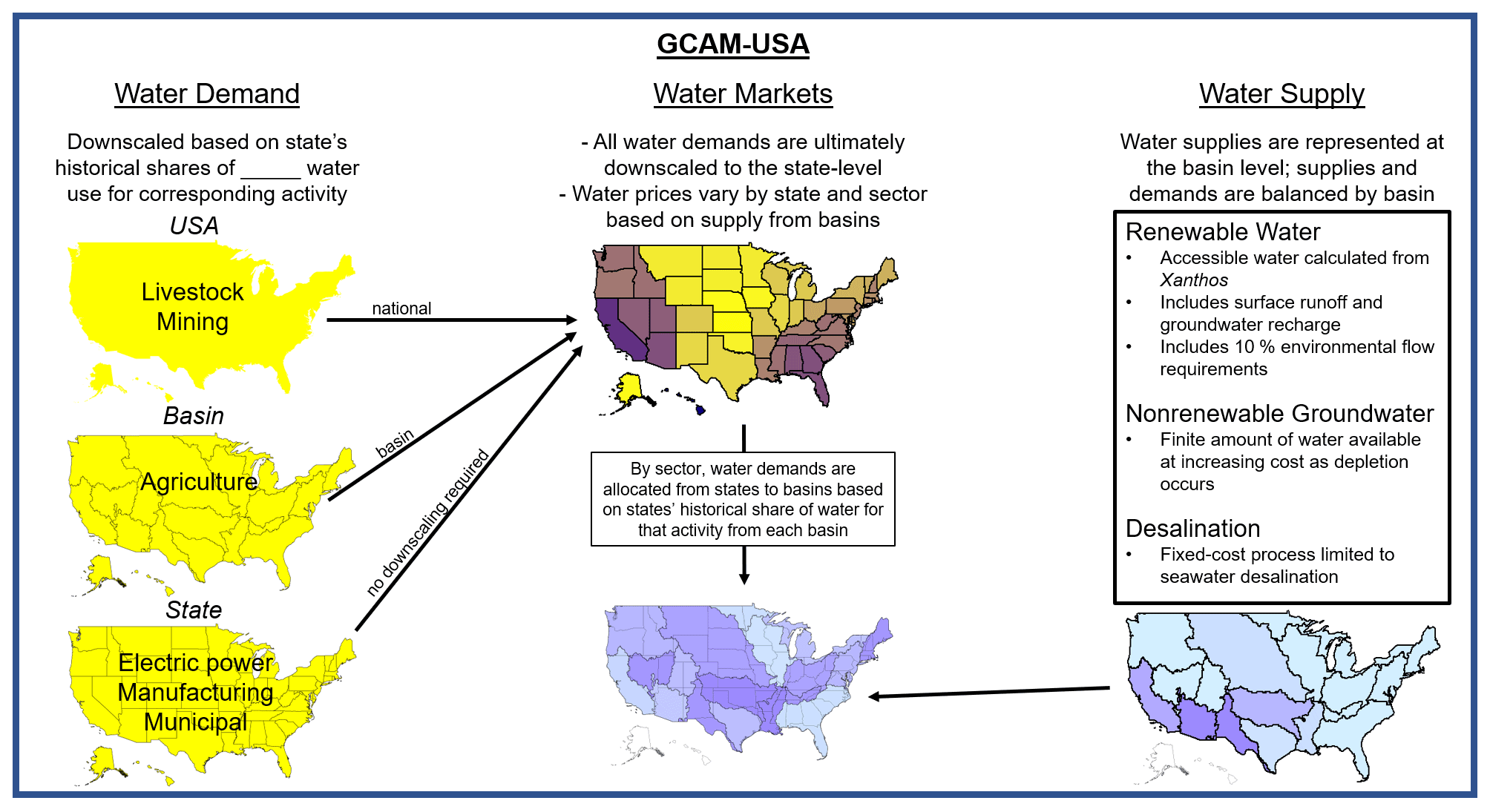
Figure 1 Conceptual diagram of GCAM-USA water market structure.

3.2 Introduction of water markets behavior (supply and demand)

3.2.1 Water supplies

GCAM-USA now includes endogenous representation of water supplies and demands at a subnational scale. Figure 1 presents a conceptual diagram outlining how (and at what scale) water demands and supplies are represented in GCAM-USA. The model represents water supplies from three distinct freshwater sources: renewable water (surface and ground), non-renewable (or fossil) groundwater, and desalinated saltwater. Additionally, saltwater is available for cooling of thermal power plants (and treated as an unlimited resource) in coastal states only. These water resources are represented at the HUC-2 river basin level and include extraction costs and availability limits for each resource type, such that water prices escalate as demand increases. The USA's water is supplied by 23 water basins, some of which are shared with neighboring regions (Canada, Mexico, and the Caribbean). GCAM's water supply system is described in detail in Kim et al. (2016) and Turner et al. (2019); a high-level overview is provided below.

Renewable water is the least expensive source of water in GCAM and includes direct extraction of surface water as well as pumping of recharged groundwater. A global hydrology model, Xanthos (Li et al., 2017; Vernon et al., 2019), is used to calculate long-term average annual streamflow for each water basin by routing gridded runoff at 0.5^∘ spatial resolution. A total of 10 % of this average annual flow is allocated to environmental flow requirements and thus unavailable; the remaining portion represents the maximum renewable water supply. A fraction of this renewable water supply is considered currently accessible at low cost via existing infrastructure for capturing, storing, and delivering; this fraction is adjusted to reflect the amount available even in dry years (henceforth referred to as “accessible volume”) (Kim et al., 2016). For most basins, this accessible volume is derived from Xanthos simulations of base flows and storage reservoirs (utilizing the Global Reservoir and Dams inventory) (Kim et al., 2016); in some basins where estimates of groundwater depletion are available, the accessible portion of renewable water is derived as the historical difference between total water withdrawals and fossil groundwater pumping (Turner et al., 2019). In model simulations, basins can withdraw greater fractions of the total renewable water supply (beyond the accessible volume) at significantly higher costs, reflecting the potential costs of interventions such as river rerouting, dam construction, or water transportation (Kim et al., 2016; Turner et al., 2019).

Each water basin in GCAM also contains a volume of potentially exploitable non-renewable groundwater, divided into several grades of increasing price based on estimated drilling and pumping costs. Total physically exploitable groundwater reserves (without considering economic and environmental constraints) are estimated at a 50 km grid scale for all major aquifers from data on aquifer areal extent, porosity, thickness, permeability, and groundwater depth as described in Turner et al. (2019) (Sect. 2.3). An extraction cost model is used to simulate groundwater pumping for each 50 km grid to estimate extraction costs including capital costs (a function of well depth and complexity), maintenance costs, and operating costs (reflecting well depth, yields, and country-specific electricity prices). Costs associated with water treatment, conveyance, and storage are not included due to lack of available data. These water quantity and cost data points are then aggregated to the HUC-2 water basin level and organized into grades of increasing cost. By default, only 25 % of physically exploitable groundwater is assumed to be available for extraction to reflect environmental limits on groundwater depletion (in the absence of a global data set facilitating basin-specific environmental factors in the model; Turner et al., 2019).

As the maximum renewable water supply is approached, non-renewable groundwater begins to become an economically competitive source of water withdrawals. However, groundwater supplies are depleted as they are exploited; non-renewable groundwater consumption leads to water price increases as each marginal unit of groundwater entails increased pumping costs. Desalinated seawater is also available in coastal basins and states (but not inland basins and states) to meet water demands excluding irrigation demands, although this is at a high price due to the energy intensity of desalination. Water prices in GCAM are incurred directly by water-consuming technologies and ultimately passed onto end users in the costs of goods (e.g., crops) and services (e.g., electricity). Thus, increasing water prices can motivate shifts to less water-intensive production methods such as rain-fed agriculture or more water-efficient power plant cooling systems.

3.2.2 Water demands

In GCAM, water demands from all sectors – primary energy (mining), agriculture (irrigation), livestock, electric power, manufacturing, and municipal – are tracked endogenously in two forms. Water withdrawal represents the total volume of water extracted from the supply system, while water consumption represents the fraction of withdrawals not directly returned to the system for immediate re-use. Water resource availability and demands (i.e., withdrawals) are endogenously resolved through a water market pricing mechanism at the river basin level.

In GCAM-USA, the drivers of water demands are modeled at multiple scales. All water demands are endogenously mapped to the state-level and resolved with water supplies at the basin level. Several water demand sectors, including electricity generation, manufacturing, and municipal water use, are represented directly at the state level. U.S. Geological Survey (USGS) historical water withdrawal data (https://water.usgs.gov/watuse/data/, last access: 1 October 2020) is used to calculate state-specific water demand coefficients for the municipal and manufacturing sectors. Municipal water demands are driven by heterogeneous state level socioeconomic trends (see Sect. 2.2.1). All states' municipal water withdrawal-to-consumption ratio is assumed to improve at a constant rate over time. Manufacturing water demands are calculated from state-level U.S. Energy Information Administration (EIA) data for industrial energy consumption for historical years (https://www.eia.gov/state/seds/seds-data-complete.php, last access: 15 May 2020), which is then matched with USGS water demand data to obtain state-specific water demand coefficients. These coefficients are held constant through the end of the century; future industrial water demands are purely a function of industrial activity at the state-level, with a presumption of no structural changes that would cause the water intensity of industry to deviate from historical levels.

In the electric power sector, GCAM-USA includes an endogenous competition between cooling systems for each thermal electricity generation technology. Broadly, GCAM-USA represents once-through, seawater (once-through), recirculating, cooling pond, dry cooling, and dry-hybrid cooling systems. Not all systems are available for every fuel and cooling technology (Table S5 specifies which fuel–cooling system combinations are available in GCAM-USA). Wind power is assumed to have no water demands (withdrawals or consumption), while photovoltaic solar (PV) requires a small amount of water for plant operations and maintenance. Hydropower has no water withdrawals but some consumption, due to evaporation losses associated with impoundment reservoirs. All other generation technologies (including concentrated solar power, or CSP) require a cooling system. Cooling system capital costs, along with the cost of providing cooling water, influence decisions about which technologies are deployed in future model periods (Liu et al., 2019); water prices also impact power sector operation decisions (see Sect. 3.3 for more detail).

Three other demand sectors – primary energy (mining), agriculture (irrigation), and livestock – are not represented at the state level in GCAM-USA. Water demands for these sectors are driven by activity at the national level (primary energy, livestock) or land use regions (irrigation; see Graham et al., 2021). Calvin et al. (2019) describes how water demands for these three sectors are calculated. These demands are then endogenously downscaled (mapped) to the states using sector-specific historical demand shares based on 0.5^∘ × 0.5^∘ gridded water demand data from Huang et al. (2018). Thus, although activities such as natural gas extraction are modeled at the national level, water demands associated with such activities are tracked at the state-level within the model via endogenous downscaling of demands based on historical shares.

Across all demand sectors, state-level water demands are mapped to the basin level (where supplies and demands are balanced). State-to-basin mappings are also conducted on the basis of Huang et al. (2018). In short, state shares of historical water demands for a given basin and sector are calculated based on Huang et al. (2018). Note that a given state or sector's water demands can be supplied by multiple basins and that multiple states' water demands for a given sector can come from a single basin. State–basin shares are held constant for future periods at their 2010 values; thus, future competition between basins to supply water for a given sector or state is pre-determined by the historical share of water demands. There is also competition within coastal state–basin combinations between natural fresh water (renewable or non-renewable) and fresh water from desalination.

With this new water market structure in GCAM-USA, users can track comprehensive water demands (withdrawals and consumption) for each region and sector. The model also outputs water supplies by water type (renewable, non-renewable, desalinated) at the basin level.

Figure 2 Conceptual diagram of new GCAM-USA electric power sector.

3.3 Increased operational resolution in the electric power sector

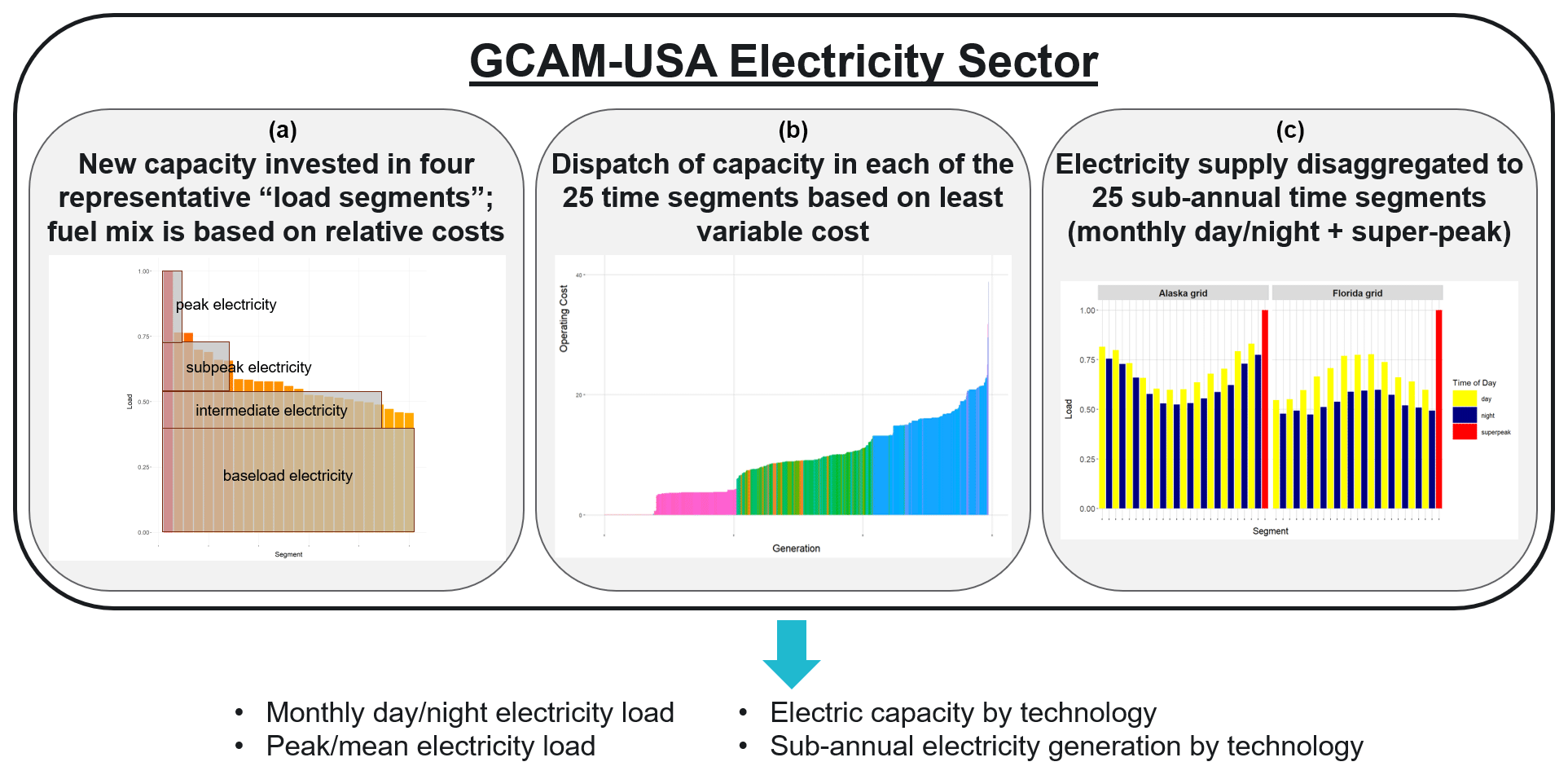
One of the most significant developments in GCAM-USA v5.3_water_dispatch is the new electric power sector (dispatch) model (Fig. 2). This model now separates long-term decisions about capacity expansion (Fig. 2a) and short-term decisions about dispatching that capacity (Fig. 2b) to meet electricity demands at sub-annual timescales (Fig. 2c). This finer-scale operational detail provides more robust results about the ability and timing of variable, or intermittent, energy sources to contribute to power supply, and requires new approaches to capture the contribution of various technologies to reserve capacity. Each of these features is described in detail below.

3.3.1 Electric power capacity investment and retirement

Economic decisions in the power sector occur on different time horizons. Capacity expansion – decisions about investing in new power plants – consider the profitability of these plants over the course of their expected lifetime, usually several decades. These decisions are in principle based on uncertain information – future fuel and electricity prices cannot be known at the time of investment. Thus, investment decisions in the GCAM-USA power sector are made using a probabilistic logit formulation that assumes a distribution of realized costs and preferences due to heterogeneous real-world conditions (Calvin et al., 2019; Clarke and Edmonds, 1993; McFadden, 1980).

Investment decisions are made in four representative “load segments” (base load electricity, intermediate electricity, sub-peak electricity, and peak electricity; Fig. 2a) corresponding to how the plant is expected to operate: for example, nuclear technologies are available for investment in the base load and intermediate segments, while gas combustion turbine technologies are invested only in the sub-peak and peak segments. Within each investment sector, various fuels (subsectors) compete for share based on relative costs using the logit choice model described above. Within subsectors, different generation technologies (i.e., conventional coal vs. integrated gasification combined cycle, IGCC, coal) compete for share of generation within a given fuel type. Finally, within each generation technology there is competition between alternate cooling systems (for thermal power plants). See Sect. 3.2.2 for a description of which cooling systems are represented in GCAM-USA.

Within the investment sectors (segments), each level of competition is based on relative levelized costs of electricity generation. These costs include power plant capital, cooling system capital, fixed operations and maintenance (O&M), variable O&M, resource inputs (fuel, water, etc.), policies (portfolio standards, emissions penalties) in place at the time of investment, and capacity credits (described in Sect. 3.3.3). Technology costs are the same across investment segments, but the capacity factors used to levelize technology costs vary by segment, corresponding to different a priori assumptions about how frequently plants in different investment segments are expected to operate. The base load segment is assumed to have the highest capacity factors and peak load the lowest capacity factors. These capacity factors will not necessarily match those which result from the capacity dispatch.

Investment decisions are made at the state level and aggregated across the four investment segments. Power sector investments are tracked by their original operating year and available to be dispatched in subsequent model periods until the end of their physical lifetimes (which vary by technology) unless the capacity is substantially underutilized and prematurely retired for economic reasons. Capacity investment requirements are calculated to ensure sufficient capacity is available to meet electricity demands across all dispatch segments in each model period, including a 15 % reserve margin. New capacity requirements are allocated across the four investment segments by mapping each investment segment to the dispatch segment whose load most closely matches the average load of the investment segment and comparing the variable cost of the marginal existing generator to the full cost of investing in a new plant. The demand for new capacity is processed in order from low to high load (base load first, peak last) so that the model knows how much capacity (including reserve margin) remains to be met by super peak (the 10 highest load hours of the year per grid region).

Existing capacity that becomes consistently too expensive to operate may be permanently retired before the end of its physical lifetime. These retirements could be driven by policies like an emissions price, sustained high fuel or cooling water input costs, or a plant being displaced by lower-variable cost technologies in the dispatch curve. When making investment decisions, the model compares the variable cost of technologies not dispatched in each representative dispatch segment to the price of the corresponding investment sector (including both fixed and variable costs) using a simple smooth function. If a technology is more expensive to operate than the costs of building and operating an average new plant in the relevant investment segment, some of that technology's capacity will retire (a greater fraction will retire as that cost delta increases). These retirement decisions are lagged by one model period; retirements each year are based on the previous period's dispatch.

3.3.2 Electric power dispatch

After new capacity investment decisions are made, all capacity (existing and newly invested) is gathered into a set of technologies available for dispatch at the grid-region level. At this point, there is no distinction among investment segments – a combined cycle gas plant is the same whether it was invested with the assumption of operating as base load or in sub-peak – although there is still a distinction among technology vintages (year of investment) because plant efficiencies and O&M costs evolve over time. Each grid region contains 25 load segments corresponding to daytime and nighttime loads for each month of the year, plus an annual super-peak containing the top 10 load hours of the year. Information on these sub-annual load profiles comes from Federal Energy Regulatory Commission form no. 714.

For each of these 25 dispatch segments, the model sorts all available capacity by variable cost (including fuel and water costs, variable O&M costs, and policy costs tied to a unit of energy or emissions production) and dispatches (operates) them based on least variable cost. Each generation technology is assigned a maximum production level for each segment, which is a function of (1) the number of hours in the segment, (2) the amount of capacity available for that technology, and (3) a “segment capacity factor”. For dispatchable technologies (nuclear, fossil fuels, biomass), the segment capacity factor is identical for each segment and reflects plant availability considering downtime for maintenance, refueling, etc. The exception to this rule is the super-peak segment, in which it is assumed that all dispatchable are available at their full capacity. For intermittent (or variable) technologies, the segment capacity factor varies by segment and reflects heterogeneous resource availability. For example, solar plants are only available during daytime segments and wind availability tends to be higher in nighttime segments. The model loops through each dispatch segment (S) and state technology vintage (T), assigning each T its maximum level of production to meet the demand in S until the full demand is met, creating a dispatch curve for each dispatch segment in the process.

The price of electricity is equal to an average of each segment's marginal generator's variable cost, plus the capacity price. By default, the load profiles in GCAM-USA are fixed over time – the distribution of annual load across the 25 sub-annual dispatch segments is calibrated to historical data for 2015 (by grid region) and fixed across future model periods. In contrast, Khan et al. (2021) utilized a version of GCAM-USA with “detailed demand segments” where the electricity load profile is distinguished by end-use sector (buildings, industry, transportation) for each grid region, and electricity from each load segment is explicitly consumed by each end-use sector. In this “demand segments” configuration, the annual load profile evolves endogenously within the model as the relative share of consumption across end-use sectors changes and as demands for thermal building services (heating and cooling, represented at the same monthly day and night temporal resolution) evolve over time. This model feature is not included in the GCAM-USA v5.3_water_dispatch.

3.3.3 Capacity markets and capacity credits

Historically, regulators and regional transmission operations have required that sufficient reserve capacity is available to minimize the probability that a shortage occurs by imposing a capacity reserve margin on electric utilities that prescribed a percentage of capacity (often 15 %) to be maintained in excess of expected peak demand. The additional cost of this reserve capacity was incorporated into the electricity rates paid by consumers. Deregulated markets also have mechanisms in place to ensure capacity reserve margin, called capacity markets. In addition to the production and sale of electrical energy in real time, capacity markets generate revenues to maintain grid reliability by paying electricity generators a premium for capacity beyond what is earned from supplying electricity. Because all generators contribute to reliability, each generator can receive revenue in the capacity market. Revenues from capacity markets can be very important for the financial viability of power plants, particularly for peak-load plants that operate for a small percentage of hours per year.

Historically, regulators and regional transmission operations have required that sufficient reserve capacity is available to minimize the probability that a shortage occurs by imposing a capacity reserve margin on electric utilities that prescribed a percentage of capacity (often 15 %) to be maintained in excess of expected peak demand. The additional cost of this reserve capacity was incorporated into the electricity rates paid by consumers. Deregulated markets also have mechanisms in place to ensure capacity reserve margin, called capacity markets. In addition to the production and sale of electrical energy in real time, capacity markets generate revenues to maintain grid reliability by paying electricity generators a premium for capacity beyond what is earned from supplying electricity. Because all generators contribute to reliability, each generator can receive revenue in the capacity market. Revenues from capacity markets can be very important for the financial viability of power plants, particularly for peak-load plants that operate for a small percentage of hours per year.

The GCAM-USA electricity dispatch model's investment segments represent demand and supply of capacity to meet peak demand plus a reserve margin. It also represents the economics of capacity markets. All generators are assumed to contribute to reserve margin and receive payments for their contributions. Dispatchable technologies can contribute their full rated capacity toward reserve margins and hence receive full payments, which assumed assumed to equal the levelized capital cost of a gas combustion turbine power plant (the least expensive dispatchable capacity to build), consistent with results from optimization models (for example, see Cole et al., 2017, Fig. 8). Due to their intermittency, renewables can contribute only a fraction of their rated capacity. In reality, this fraction – also known as the capacity credit or capacity value (CV) – is a function of the correlation between the temporal generation pattern of the resource and the peak load periods, as well as the fraction of intermittent generation compared to total regional output. As wind or solar constitute more of the system capacity, the variability of their peak-load operation will have a decreasingly beneficial effect on system reliability; hence, the capacity value of a renewable technology decreases with its penetration. We model this decreasing capacity credit as a function of renewable energy (VRE) capacity shares using a simple sigmoid function. Wind power receives a 15 % capacity value, but this credit is largely unaffected by the level of wind penetration; solar power receives 40 % of the capacity credit at low levels of penetration, but this capacity value decreases to 5 % by the time solar constitutes 20 % of overall capacity (Cole et al., 2017).

In addition to decreasing capacity credits, VRE technologies may also face decreasing capacity factors as deployment increases because locations with the strongest resources (solar insolation or wind speed) will tend to be utilized first, and subsequent installations will be cited in locations with marginally poorer resources. Section S2 describes how the GCAM-USA electricity dispatch model captures these dynamics.

The new GCAM-USA electric power sector provides a rich set of outputs for each scenario. Users can track electric capacity by technology (both existing capacity and new investments); monthly day and night electricity load and electricity generation by technology; variable costs and electricity dispatch order by monthly day and night electricity load segment; dynamically evolving technology capacity factors (as each technology-vintage's operation evolves over time). Most of these results are available at the state level, although some of the decisions (e.g., electricity dispatch order) are represented at the grid region level.

4 GCAM-USA Reference scenario storyline

Human–Earth system models simulate outcomes of dynamic systems whose future evolution is highly uncertain. For this reason, it is important to articulate a clear storyline, or “narrative description…highlighting the main scenario characteristics, relationships between key driving forces, and the dynamics of their evolution” (IPCC, 2014) (p. 1773), about the evolution of the modeled system. This high-level description of drivers and trends provides the basis for clearly documenting assumptions, including choices about model structures and parameters, which may influence future model outcomes (Binsted et al., 2020). The following section outlines the storyline for the GCAM-USA Reference scenario. Additional description of the GCAM-USA Reference scenario storyline is available in the online GCAM-USA model documentation page (http://jgcri.github.io/gcam-doc/gcam-usa.html, last access: 22 October 2022).

4.1 Socioeconomics and end-use energy demands

The GCAM-USA Reference scenario assumes a steadily growing US economy and growing but gradually peaking population through the end of the century. A detailed description of GCAM-USA's default socioeconomic assumptions is provided in Sect. 2.2.1. This population and economic growth translates to increasing service demands in all end-use sectors. The GCAM-USA Reference scenario assumes a continuation but not an expansion or strengthening of current energy efficiency policies (e.g., building efficiency standards). In aggregate, total final energy demands increase as efficiency improvements are slower than increases in demand for end-use energy services (space heating and cooling, passenger and freight transportation, industrial energy use, etc.), although the balance between population and income driven demand growth and service efficiency vary by sector. (Section S3 provides information on service and energy growth by sector for the GCAM-USA Reference scenario.) End-use sectors tend to become increasingly electrified over time, with the trend strongest in buildings (where many new energy demands come from electronic devices). Transportation remains reliant on liquid fossil fuels, although light-duty vehicles (LDVs) electrify more rapidly than the sector as a whole.

4.2 Electric power

In the GCAM-USA Reference scenario, electricity demand grows slowly but steadily over the next 3 decades, reaching approximately 5600 TWh in 2050. Load grows slightly faster over the second half of the century, reaching 7700 TWh in 2100. This demand is driven by increased electrification in buildings and industry, with modest growth in transportation after 2050. The GCAM-USA Reference scenario does reflect existing policies to incentivize battery electric vehicle (BEV) deployment. This future load growth departs from recent historical trends; USA electricity demand increased only 4 % in the decade between 2009 and 2019 (EIA, 2020a).

In terms of electricity supply, rising electricity demand is met by increasing generation from natural gas and renewables in the GCAM-USA Reference scenario. Growth in gas generation dominates through 2050, with moderate increases in wind and solar; post-2050, gas generation flattens while wind and solar growth accelerate substantially. The GCAM-USA Reference scenario assumes no new deployment of coal-fired power plants without carbon capture and storage (CCS), based on the Clean Air Act Section 111 (b) New Source Performance Standards (Environmental Protection Agency, 2015). Coal generation remains roughly flat from 2020 to 2030 and remains a substantial portion of the generation mix through 2040, until much of the capacity reaches the end of its technical lifetime. New nuclear deployment does not occur in the GCAM-USA Reference scenario until 2030, considering the long lead time for permitting and construction and the dearth of nuclear plants currently under construction in the USA (apart from Vogtle Units 3 and 4 in Georgia). A more detailed description of the GCAM-USA Reference scenario storyline for the electricity sector is available in Binsted et al. (2020).

4.3 Water

At a national level, the GCAM-USA Reference scenario entails modest declines in water withdrawals through mid-century, with relatively flat water demands thereafter. The decline in demand is driven by a reduction in power sector cooling water. Despite growing electricity demand, the gradual retirement of plants with once-through cooling systems (which are assumed to be unavailable for installation in future model periods) coupled with a shift towards less water-intensive generation technologies (e.g., natural gas, renewables) results in diminishing power sector water demands in the GCAM-USA Reference scenario.

Declining power sector cooling water demands are partially offset by increased withdrawals from the agriculture, livestock, manufacturing, and municipal sectors; these demands are largely driven by economic growth. Per-unit water requirements for primary energy, livestock, and manufacturing are assumed to be constant through the end of the century, and thus the scale of those activities corresponds directly to water withdrawals. In the agricultural sector, there is a competition between irrigated and rainfed crop management systems; however, in the US, most agriculture is already irrigated, and the GCAM-USA Reference scenario assumes no improvement in crop-specific per-unit irrigation water requirements over time. Municipal water use does become somewhat more efficient over time, but these efficiency improvements are offset by population growth.

4.4 Land

Agricultural productivity increases gradually in the US in the future, with crop-specific annual productivity growth rates ranging from 0 % yr⁻¹ to 0.67 % yr⁻¹ between 2015 and 2100. These productivity gains represent exogenously specified technical change, which varies by crop, management practice (irrigated vs. rainfed, high vs. low fertilizer application), and year, reflecting factors like improved mechanization, and crop breeding. Alternate fertilizer use and irrigation practices are represented endogenously and respond dynamically to economic forces (commodity prices, land values, input costs, etc.) within the model; shifting management practices generate additional productivity changes beyond those listed above.

Demand for agricultural commodities increases in the GCAM-USA Reference scenario, driven by changes in population, income, and biofuels demand. Per capita food demand is relatively flat in the US given its income level, with staple demand decreasing slightly over the century and non-staple demand increasing modestly (Edmonds et al., 2017). Demand for liquid biofuels increases by 160 % between 2015 and 2050 in the reference scenario. The US is a net exporter of crops, with ∼ 21 % of all crops produced exported in 2015 and ∼ 25 % exported in 2050 in a reference scenario.

Table 1 Scenario design

5 Scenarios

The following section presents results for four illustrative scenarios constructed using GCAM-USA v5.3_water_dispatch. The scenarios vary across the following two dimensions: socioeconomic drivers and energy system evolution. These scenarios, outlined in Table 1, are intentionally simple and designed to illustrate key model behavior and capabilities across a range of potential futures; they are not intended to reflect “likely” outcomes or detailed narratives of future worlds.

The Ref scenario is the default GCAM-USA Reference scenario based on the storyline described in Sect. 4. In this scenario, population and GDP growth assumptions are consistent with SSP2 (see Sect. 2.2.1 for more information on socioeconomic assumptions in GCAM). The High Growth scenario assumes faster population and economic growth consistent with SSP5. Note that although the SSPs are global scenario narratives, our High Growth scenario assumes that only the US population and economy grows at the accelerated SSP5 rates, in order to isolate the impact of economic growth in the US on model outcomes.

The Transition scenario contains default (reference) socioeconomic assumptions but reflects a transition towards a lower-carbon energy system (reaching zero energy system carbon dioxide emissions by 2090; see Fig. S1 in the Supplement for scenario emissions pathways). The energy transition is implemented via a price on carbon dioxide emissions from the energy system of roughly USD 22 per t CO₂ (2015 USD values) beginning in 2025 and escalating at 5 % yr⁻¹ thereafter. The Transition scenario does not include any new or improved technology options that are not available in the Ref scenario (only shifting technology deployment in response to the carbon price); it also does not explicitly reflect any “lifestyle” changes that could impact future energy demand (although end-use energy consumption responds endogenously to changes in energy prices). Finally, the High Growth + Transition scenario combines the higher growth (SSP5) scenario element with the transition towards a lower-carbon energy system.

In all scenarios, water availability is constrained to default levels of renewable and non-renewable groundwater as described in Kim et al. (2016) and Turner et al. (2019). The methods for constructing GCAM's renewable water and groundwater resource curves are described in Sect. 3.2.1 (water supplies). In short, this entails a 10 % environmental flow restriction on renewable water, renewable water availability based on the stable volume of long-term average annual flow (i.e., not reflecting potential impacts of future climate change on water availability), and a 25 % limit on physically exploitable groundwater extraction reflecting environmental limits on groundwater depletion. Renewable water and groundwater resource curves by river basin are included in Fig. S4. Water prices will thus vary by basin; basins in which renewable water supplies exceed water demand will have negligible water prices, but as demands rise in the future across scenarios, some basins may need to utilize and non-renewable groundwater (and possibly desalinated water), raising the price of water and motivating a shift towards less water-intensive technologies.

6 Results

This section presents results for the four GCAM-USA scenarios described above, focusing on model outputs for energy consumption (Sect. 6.1), electric power (Sect. 6.2), water (Sect. 6.3), and land use (Sect. 6.4). Each system will begin with a description of high-level national-aggregate trends but focus mainly on subnational detail within the model. The section concludes with a brief comparison to historical data and other future scenarios (Sect. 6.5).

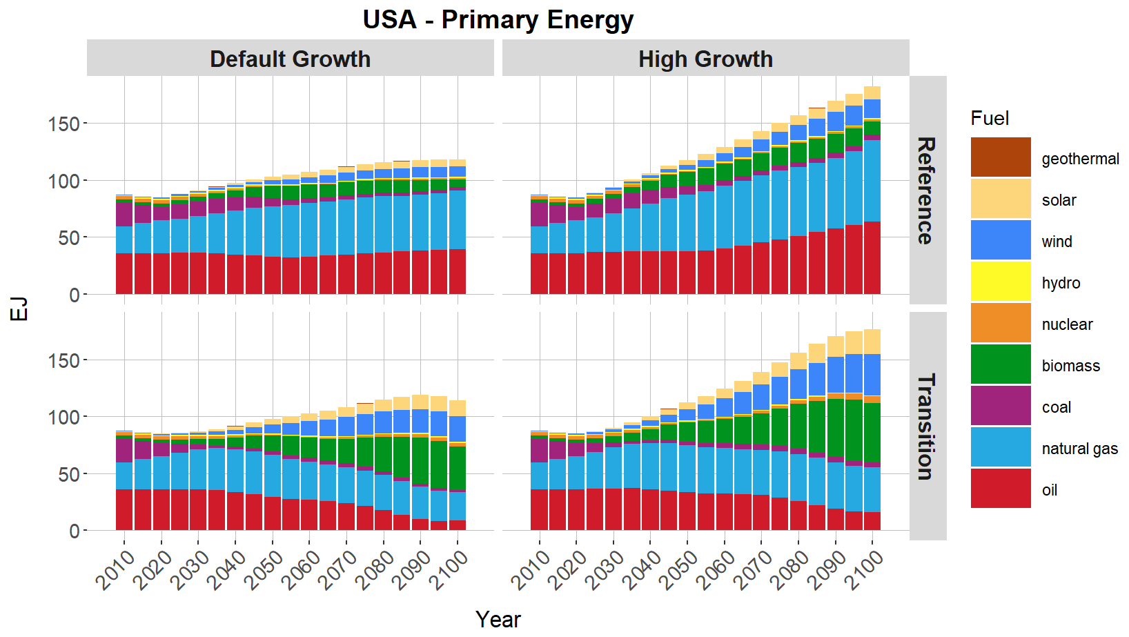
Figure 3 US primary energy consumption (national total) by fuel and scenario. Columns reflect alternate assumptions about socioeconomic drivers; rows represent alternate assumptions about energy system evolution.

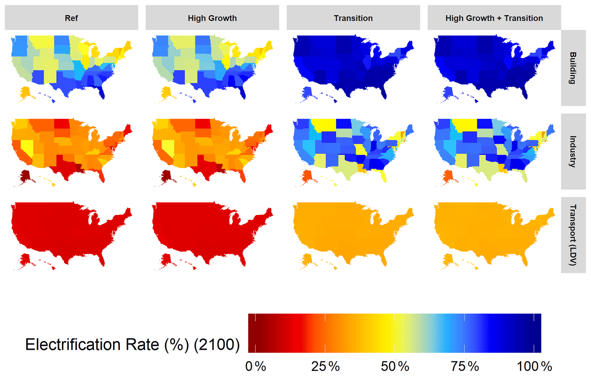
Figure 4 Electricity share of final energy by state, scenario, and end-use sector (building, industry, passenger vehicles) in 2100. Note that because electric drivetrains are more energy efficient than internal combustion engines, the share of passenger transportation service provided by electricity (BEVs) in the scenarios will exceed the energy consumption shares shown in this figure. A plot of passenger vehicle electrification by share of transportation service (passenger miles traveled) is provided as Fig. S2.

6.1 Energy consumption

The four GCAM-USA scenarios presented in this paper entail vastly different future energy trends (Fig. 3). In the Ref scenario, total primary energy for the USA grows steadily throughout the century, with the energy mix dominated by fossil fuels. Oil consumption is relatively flat from 2015 to 2100; coal demand dwindles past 2050, while natural gas becomes the largest source of primary energy, with consumption nearly doubling in 2100 (relative to 2015 levels). The fuel trends are similar in the High Growth scenario, but total primary energy more than doubles in 2100 (relative to 2015), compared to only 38 % growth in the Ref scenario over the same period.

In the Transition scenario, the decline of coal happens sooner (mostly eliminated by 2035), while oil consumption is roughly flat through 2040 before declining in the second half of the century. Gas consumption grows over the next several decades but peaks by 2050. Bioenergy, wind, and solar consumption grow relatively slowly through 2050 and rapidly thereafter; by 2100, these three fuels constitute nearly two-thirds of total US primary energy consumption. The Transition + High Growth scenario has similar trends, but primary energy demands are more than 50 % greater in 2100.

Beneath these national-level results is significant heterogeneity in outcomes across states and sectors. Figure 4 shows the electrification rate (electricity share of final energy) by sector for each scenario in 2100. Across all scenarios, the building sector tends to be the most electrified, although there is significant regional variation. In the Ref scenario, building sector electrification ranges from 36 % (Vermont) to 90 % (Florida) in 2100; electrification rates are similar in the High Growth scenario, although they tend to be slightly higher. The wide range of building electrification rates is driven by several factors. Differences in the energy service profile of the buildings sector vary by region; for example, southern states require more air conditioning (powered by electricity) and little heating, while northern states require little cooling but substantial space heating (often provided by gas, heating oil, or biomass, as well as some electricity). Historically estimated differences in fuel preferences for different services (e.g., electricity vs. gas (or other fuels) for space heating, water heating, cooking) by state are carried forward and influence future technology choices (GCAM-USA's calibration routine is discussed in Sect. 6.5.), as do regionally differentiated fuel prices (oil, gas, coal, and electricity prices all vary by grid region).

This range in building electrification tightens substantially in the Transition scenario. Electrification of end-use sectors is a key emission-reduction strategy in response to the carbon price in the Transition scenario; buildings, the most electrified sector in the Ref scenario, tends towards the upper end of electrification, with electricity accounting for 79 % of building energy consumption in New York and 97 % in Florida. With fossil fuel technologies facing a substantial price on the CO₂ emissions they generate in the Transition scenario and electric options available for every building service, deep electrification of the buildings sector occurs across states by 2100, although some differences remain due to variations in regional preferences, fuel prices, and turnover rates of existing equipment stock.

Industry electrification rates are similarly diverse. In the Ref scenario, electricity accounts for between 2 % (Alaska) and 50 % (Nevada) of industrial energy use. Again, these rates are similar in the High Growth scenario, although the magnitudes of this electricity consumption are vastly different. For example, Ohio's industry sector has a 31 % electricity share in Ref and a 32 % share in High Growth, but the sector consumes 95.3 TWh in Ref compared to 158.3 TWh in High Growth. As with the building sector, industry electrifies quite substantially in the Transition scenario, although there is more heterogeneity in these outcomes. For example, Alaska has only a 22 % industrial electrification rate in 2100, while Alabama has an 86 % electrification rate (Transition scenario). GCAM-USA's industry sector is represented at a more aggregate level than buildings, but the same basic factors – state-specific fuel preferences, capital stock accumulation, and regionally differentiated fuel prices – drive differences in industrial fuel mix across the states. Additionally, some states, such as those with large petrochemical sectors (e.g., Louisiana, Texas), use much of the energy in industry as feedstocks, which lowers the share of electricity in their industrial energy mix.

Electrification of passenger transportation is much more regionally homogenous than other sectors. In the Ref scenario, between 11 % (Texas) and 14 % (Hawaii) of states' passenger transport energy consumption comes from electricity. These rates are virtually identical in the High Growth scenario. In the Transition and Transition + High Growth scenarios, these electrification rates range from 33 % to 40 %. This represents a significant increase in electrification relative to the Ref and High Growth scenarios, although the range of outcomes is fairly small. There are several reasons for this. First, because electric vehicle (EV) penetration is very low in the historical period (2015), the model has little information about varying regional preferences for EVs around which to calibrate. Second, since these consumer preferences for EVs begin from a similar place (near zero deployment), these preferences tend to evolve homogenously over time in the model. Third, vehicle costs and emission costs are the same in every state in these scenarios; the scenarios do not represent existing state-level zero-emissions vehicle (ZEV) mandates. Finally, although GCAM-USA does capture regional differences in fuel prices (for both traditional liquid fuels and electricity), fuel prices tend to represent a small percentage of total vehicle ownership costs; thus, these fuel price differences do not impact transportation results as much as they may in other sectors. Additional information about the reference transportation assumptions in GCAM-USA v5.3_water_dispatch, as well as how alternate assumptions of state-level policy or consumer preferences could be implemented, is provided in Note 4 in the Supplement.

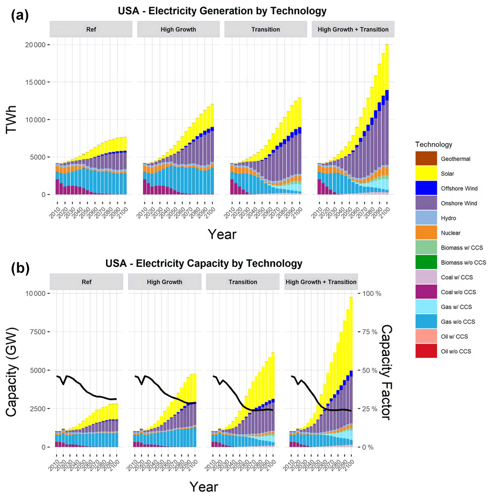
Figure 5 USA electricity generation (a) and capacity (b) by technology and scenario. Lines on capacity plots (b) represent national fleet average annual capacity factor and correspond to the secondary (right) y axis.

6.2 Electric power

GCAM-USA now explicitly tracks both electricity generation and generation capacity by technology and cooling system. Figure 5 presents both electricity generation and capacity for our four GCAM-USA scenarios. Electricity generation in the Ref scenario grows 85 % over the course of the century (relative to 2015) to nearly 7700 TWh, while capacity grows more than 250 % to over 2800 GW in 2100. Fossil fuels dominate the generation mix in the near- to medium-term, with coal generation gradually declining and gas generation steadily growing. By 2060, fossil fuels account for just over 50 % of total US power generation, with wind and solar the next most significant generation sources (behind natural gas). Hydropower is exogenously specified in GCAM-USA and fixed at 2019 levels for all historical periods. Nuclear power represents a significant portion of the generation mix through about 2035, then dwindles for several decades (driven by an assumption of 60-year operational lifetimes) before growing again beginning around 2070. Capacity trends by fuel are similar, although wind and solar make up a larger share of capacity than generation due to their relatively low capacity factors (compared to other technologies like gas combined cycle and nuclear). The increasing penetration of wind and solar is one reason that the national fleet's annual average capacity factor declines steadily from 45 % in 2015 to 31 % in 2100. Wind and solar constitute greater than 50 % of power sector capacity by 2055, but do not account for 50 % of electricity generation until 2080.

Fuel mix trends, in both generation and capacity, are similar in the High Growth scenario. However, electricity demand in the High Growth scenario is 57 % higher than in Ref, with electricity in generation in 2100 exceeding 12 000 TWh (290 % higher than 2015 levels). Capacity growth, outpacing generation, approaches 4800 GW, more than quadruple 2015 levels. The Transition scenario, with middle-of-the-road population and economic growth but strong incentives to electrify end-use sectors to reduce their carbon intensity, sees even higher electricity growth, with generation reaching 12 900 TWh in 2100 and capacity reaching 6140 GW. In this scenario, coal phases out even more quickly, while gas peaks in 2035 and declines steadily thereafter (although gas continues to provide nearly 10 % of electricity generation in 2100, most of which is in combination with carbon capture in storage, CCS). Wind and solar constitute 50 % of total electricity generation by 2050 in the transition scenario and over 75 % in 2100, while nuclear power also contributes about 5 % of total generation in 2100. Again, the fuel mix in the High Growth + Transition scenario is similar to that of High Growth, but total electricity generation is 50 % higher in the former (nearly 20 000 TWh in High Growth + Transition vs. 12 900 TWh in High Growth), with total power sector capacity exceeding 9700 GW in 2100.

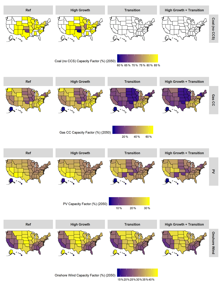
Figure 6 USA power sector capacity factor by scenario for select technologies in 2050. Note that color scales differ between technologies. No shading (white) indicates zero capacity in that state, period, and scenario.

The new electricity dispatch model in GCAM-USA also allows us to explore changes in the operation of power plants at the state-level. Figure 6 shows the endogenous capacity factors for four key technologies (coal without CCS, gas combined cycle (gas CC), photovoltaic solar (PV), and onshore wind) at the state level across all four scenarios in 2050. Note that the color scales differ between technologies. These results highlight the state-level heterogeneity in GCAM-USA – technology capacity factors (utilization rates) span a relatively wide range across states. In the Ref scenario, coal (without CCS) capacity factors range from 66 % to 85 %, although 23 state-level regions have no coal capacity in 2050. Gas CC capacity factors in the Ref scenario range from 21 % (Missouri) to 66 % (Washington) in 2050, with a national average of 49 %. PV capacity factors range from just 5 % (Alaska) to 31 % (Arizona) (22 % national average), while wind capacity factors range from 14 % (Hawaii) to 44 % (Kansas) (36 % national average).

As observed with other rate variables, these endogenous technology capacity factors tend to be quite similar in the High Growth and Ref scenarios, particularly in 2050 when deployment of intermittent technologies is still more limited. Coal plant utilization is nearly identical in the High Growth and Ref scenarios, although a handful of Midwest and Great Plains states have slightly diminished (1 %–10 %) coal capacity factors as wind deployment increases. Gas CC plants are operated between 2 % more frequently (Montana) and 5 % less frequently (Washington) in the High Growth scenario (compared to Ref) in 2050. PV and onshore wind capacity factors are consistently lower in the High Growth scenario (compared to Ref), but the differences do not exceed 1.3 % in 2050. By 2100, however, PV and onshore wind capacity factors in the High Growth scenario diverge more and are noticeably lower than in Ref. PV capacity factors are up to 7.6 % lower (New Mexico, 10.4 % vs. 17 %) in 2100, with the national average PV capacity factor about 1.4 % lower. Similarly, onshore wind capacity factors are up to 5 % lower in 2100 (New Jersey), with the national average 1.4 % lower in High Growth (compared to Ref). These declines occur because the highest quality sites for variable energy (wind and PV) are utilized first. Deployment of these technologies is significantly higher in the High Growth scenario in 2100; these additional wind and PV installations are built in increasingly marginal areas with diminishing capacity factors.

A similar and indeed exaggerated result is observed in the Transition and High Growth + Transition scenarios. PV capacity factors in the Transition scenario range from 4 % (Alaska) to 27 % (Utah) in 2050 – between 0 % and 20 % lower than those in the Ref scenario. The national average PV capacity factor is about 2.2 % lower in Transition (19.6 %) compared to Ref (21.8 %) in 2050. Interestingly, PV capacity factors are not further degraded in the High Growth + Transition scenario, still ranging between 4 % and 27 %.

Onshore wind capacity factors in the Transition scenario (2050) range from 14 % (Hawaii) to 43 % (Alaska) with a national average of 36 %. These capacity factors are again lower than those observed in the Ref scenario; greater deployment reduces the national average onshore wind capacity factor in the Transition by an additional 0.5 % relative to the High Growth scenario. Contrary to PV, combining the high socioeconomic growth and energy system transition assumptions leads to further degradation of onshore wind capacity factors, which are between 0 % and 2.6 % lower in the High Growth + Transition scenario (relative to Transition).

Gas CC capacity factors drop in the Transition and High Growth + Transition scenarios (relative to Ref) because the emissions price used to incentivize a shift towards a lower-carbon economy makes operating gas CC plants relatively more expensive. At the national level, gas CC (without CCS) capacity factors drop from roughly 49 % in 2050 (Ref) to 32 % (Transition); at the state level, these differences range from 2 % higher in the Transition scenario (Mississippi) to 44 % lower (Washington) relative to Ref. Coal power plant operations are even more strongly impacted because they are more carbon intensive; in the Transition scenario only six states have remaining coal capacity (without CCS) by 2040, and all coal capacity without CCS is retired by 2050.

An interesting regional pattern which emerges is that gas CC capacity factors tend to be higher in the southeastern states, especially in the Transition and High Growth + Transition scenarios. The southeast has relatively poor wind resources, as indicated by the low capacity factors for onshore wind. For example, in 2050 wind accounts for just 2.1 % of total capacity (1.1 % of generation) in Georgia in the Ref scenario; in the Transition scenario, this increases to only 5.0 % of capacity and 3.2 % of generation. At night, with no solar generation and a dearth of wind generation (which tends to be stronger at night), the southeast must rely on other technologies – often gas CC – to support nighttime loads. This keeps gas CC capacity factors high in the southeast compared to other regions.

Broadly, national average electric capacity factors decrease across all scenarios (Fig. 5), driven by greater penetration of intermittent renewable technologies (wind and solar), which have lower maximum availability rates. The competition for investment in new generation capacity is based on levelized generation costs (including capital, operations and maintenance, fuel costs, and emissions penalties). Despite their lower capacity factors, wind and solar account for a large share of new installations in all scenarios due to their low operating costs, lack of emissions (and associated costs), and rapidly improving capital cost. Wind and solar are especially economical in the Transition and High Growth + Transition scenarios where fossil fuel technologies face a carbon price on their CO₂ emissions.

Wind and solar capacity factors themselves decline a bit over time across all scenarios (Fig. S3 presents national average electric technology capacity factors for all scenarios and model periods); this reduction is a bit more pronounced in the Transition and High Growth + Transition scenarios (where wind and solar deployment is greatest). This is because wind and solar resource bases are finite and heterogeneous in quality; GCAM-USA assumes that the highest quality (highest capacity factor) resources are utilized first, and thus increased deployment over time entails exploiting lower-quality resources and thus diminished capacity factors (Note 2 in the Supplement explains this dynamic in greater detail). The overall (national average) reduction in capacity factor is small (2.2 % and 1.9 % reduction in PV and onshore wind capacity factors in 2050 for the Transition scenario, relative to Ref), although some states see larger reductions.

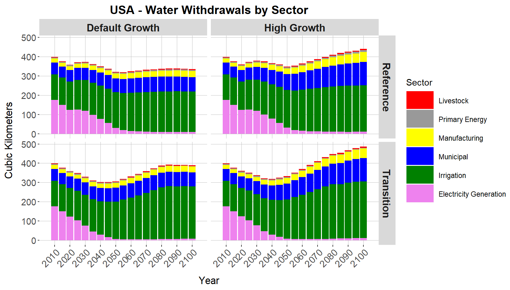
Figure 7 USA water withdrawals by sector and scenario. Columns reflect alternate assumptions about socioeconomic drivers; rows represent alternate assumptions about energy system evolution.

Capacity factors for fossil fuel (coal and gas) technologies without CCS also decrease in the Transition and High Growth + Transition scenarios because the price associated with their CO₂ emissions makes them less economical to operate (as noted above). In the new GCAM-USA electricity dispatch model structure, capacity is operated in order of least variable (operating) cost, including variable O&M, input (fuel and water) prices, and emissions penalties. However, not all technologies experience a reduction in capacity factor in the Transition scenario (Fig. S3). Bioenergy with CCS capacity factors are stable in the Transition scenario; nuclear capacity factors decline through mid-century as intermittent renewable capacity increases (nuclear has fuel costs and variable O&M costs that exceed those for solar and wind) but stabilizes from 2050 onward. Fossil technologies with CCS see steadily declining capacity factors over the course of the century as renewable penetration grows and carbon prices steadily increase (making these as fossil plants with CCS more costly to operate, as these technologies still produce some residual CO₂ emissions that escape capture).

6.3 Water

GCAM-USA now provides a comprehensive accounting of water use (withdrawals and consumption) at the state level. Figure 7 presents a time series of water withdrawals by sector for each scenario. In 2015, cooling water for electricity generation is the largest source of water withdrawals at the national level, followed closely by agricultural irrigation. Together these sectors account for more than 290 km³ of water withdrawals, or more than three-quarters of national withdrawals in 2015. However, while electricity sector withdrawals remain relatively flat through 2030 before declining rapidly to under 20 km³ by 2060 in all scenarios (and remaining low thereafter), irrigation water withdrawals grow steadily over the century across all scenarios, reaching 210 km³ in 2100 in the Ref scenario (a 49 % increase over 2015).

Growth in agricultural water withdrawals in the Ref scenario is driven primarily by cropland expansion (Fig. 10) to meet increasing food demand caused by growing population and GDP. Nationally, cropland irrigation shares (the percentage of cropland that is irrigated as opposed to rainfed) for food and feed crops increase marginally over time across scenarios (16.4 % in 2015, 17.4 %–19.6 % in 2100), albeit with substantial variation across basins and crop types. Irrigation water demands are influenced by several factors, including agricultural land area (driven by food demand and modulated by competition between cropland and alternate land uses), competition between different crop types (which have different profit rates and water requirements), and competition among production strategies (irrigated vs. rainfed and high vs. low fertilizer application) based on their costs (including water and fertilizer prices), yields, and profitability (crop prices). Irrigated agriculture entails higher costs (equipment + water costs) but achieves higher yields.

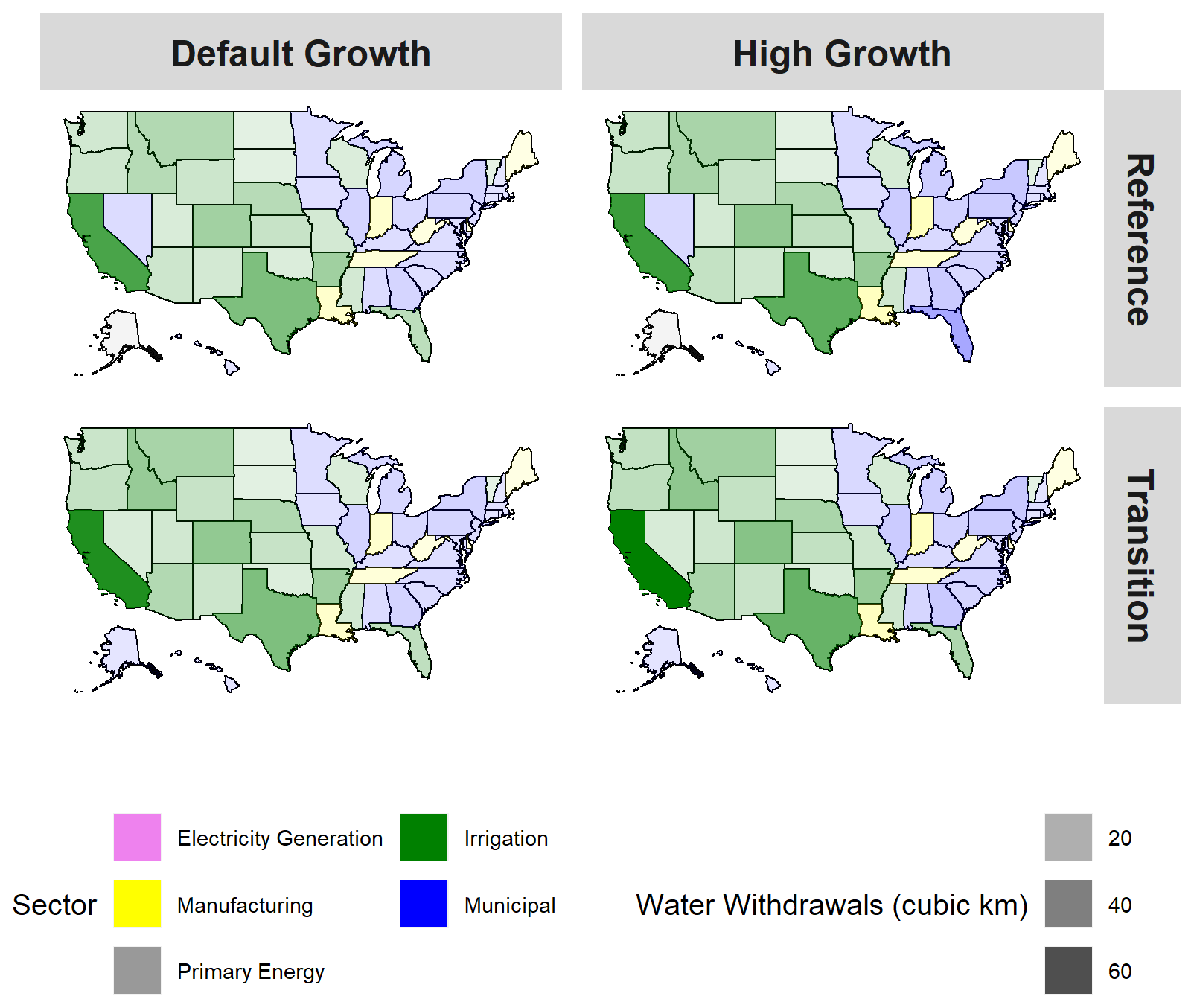
Figure 8 Water withdrawals by state and scenario in 2100. Fill color represents the sector with the largest water withdrawals in each state. Shading (transparency) corresponds to the magnitude of total withdrawals (sum of all sectors) by state. Columns reflect alternate assumptions about socioeconomic drivers; rows represent alternate assumptions about energy system evolution.

In the High Growth scenario, agricultural water withdrawals grow more rapidly to 240 km³ in 2100. In the Transition and High Growth + Transition scenarios, agricultural withdrawals reach 271 and 295 km³ in 2100, respectively. This increase in demand for irrigation water is largely driven by increased demand for bioenergy crops by the energy system. Bioenergy crops can be produced with the same four production strategies (combinations of irrigated vs. rainfed and high vs. low fertilizer application) as other crops. Irrigation shares are generally lower for bioenergy crops than they are for traditional (food and feed) crops (between 8 %–11 % across scenarios and model periods), but bioenergy cropland expands tremendously in the Transition scenario, while traditional cropland grows minimally, as described in Sect. 6.1. As a result, about 71 % of the increase in irrigation water withdrawals in 2100 (relative to 2015) are attributable to bioenergy crops rather than food and feed crops.

Municipalities are the third largest water user in terms of withdrawals, both historically and throughout the century across all four GCAM-USA scenarios. Municipal water demands grow steadily with socioeconomic growth, as do demands from manufacturing, the fourth-largest source of water withdrawals nationally. Water demands for the mining (primary energy) and livestock sectors are relatively small from a national perspective across all scenarios. In total, national water withdrawals decline slightly to mid-century in the Ref scenario and are relatively flat thereafter, with end-of-century withdrawals about 10 % lower than historical (2015) levels. In the High Growth scenario, the decline in electric power water withdrawals is more rapidly offset by increasing demands from agriculture and municipalities, with total USA withdrawals reaching 440 km³ in 2100 (nearly 20 % higher than 2015 levels). Although irrigation water withdrawals grow even more rapidly in the Transition scenario (as highlighted above), municipal and manufacturing demands remain close to Ref levels; in turn, total water withdrawals are slightly lower by end-of-century in the Transition scenario (relative to High Growth) at just about 390 km³ in 2100. The High Growth + Transition scenario has by far the largest water withdrawals in 2100 (at 486 km³), although total withdrawals in 2050 are only 3 % higher than the Ref scenario; in the near-to-medium term, growth in irrigation and municipal withdrawals (driven by increased demand for bioenergy crops and socioeconomic growth, receptively) is offset by faster declines in power sector water withdrawals due to less frequent operation of fossil fuel power plants (particularly coal, which requires substantial cooling water) and greater investment and generation from wind and PV (which have no cooling requirements).

However, as observed in the energy and electricity results, significant regional heterogeneity undergirds these national trends. Figure 8 presents water withdrawals by state and scenario in 2100; the map is color-coded according to which sector is the largest water user (in terms of withdrawals) in each respective state, while the shading of that color is scaled to total water demands (across all sectors) in the state; states with the highest water withdrawals appear most saturated. Irrigation accounts for the most water withdrawals nationally in 2100 and is also the largest water user in 22 states (mostly across the Great Plains and western US). Municipalities are the largest water users in 21 states (mainly along the eastern seaboard and Great Lakes), while manufacturing accounts for the most water withdrawals in six states. The regional distribution of water demands by sector is similar in the High Growth scenario, although municipal water use becomes larger than irrigation in Florida, and demands are generally higher across the board. Similar outcomes are observed in the Transition and High Growth + Transition scenarios, with water withdrawals increasing in volume but the sectoral distribution by state (in terms of highest consuming sector) remaining relatively stable.

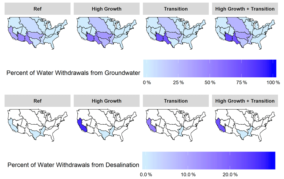
Figure 9 Percentage of total water withdrawals met by groundwater extraction (top row) and desalination (bottom row) by water basin and scenario in 2100.

In addition to water use (withdrawals and consumption), GCAM-USA also reports water supplies by source by water basin. Figure 9 presents the percentage of total water withdrawals supplied by groundwater (top panel) and desalinated water (bottom panel) in 2100 (the remaining withdrawals come from runoff, which is not included in the figure). In the Ref scenario, groundwater accounts for less than 10 % of water withdrawals in most (15 of 20) water basins, although groundwater supplies between 25 %–40 % of water withdrawals for the Arkansas White Red, California River, and Mexico Northwest Coast basins, while the Rio Grande and Lower Colorado basins rely on groundwater for nearly 50 % of their total withdrawals. The shadow prices of water for each river basin and scenario are included in Fig. S5; broadly, we observe increasing water prices in basins and scenarios with high reliance on groundwater extraction or desalination. Note that GCAM-USA's water prices represent a shadow price on water (Bierkens et al., 2019) – the intention is not to predict real-world consumer prices, but to reflect water scarcity and provide a price signal to water-consuming sectors when basins face water scarcity and marginal water demand must be met by expensive ground water extraction or desalination (where available). Results are generally consistent in the High Growth scenario; the groundwater reliant regions from the Ref scenario become slightly more groundwater reliant, and the Lower Mississippi River, Missouri River, and Texas Gulf Coast basins approach or exceed 20 % of withdrawals from groundwater. The most notable change in this scenario, however, is the California River basin, which has virtually no groundwater extraction in 2100. This is a result of over-extraction in previous model periods; by 2100, remaining groundwater is limited and is expensive to access. The California River basin thus becomes more reliant on desalination in the High Growth scenario, with nearly 30 % of water withdrawals provided by desalination (no other basin exceeds 1 %, and most do not utilize desalinated water at all). The Transition and High Growth + Transition scenarios have similar spatial patterns of water stress; the southwestern US becomes even more reliant on groundwater in these scenarios, with the Lower Colorado River and Rio Grande basins both relying on groundwater for roughly three-quarters of their withdrawals in 2100 across both scenarios. This result is tied to an expansion of agriculture in the region, discussed further in the next section.

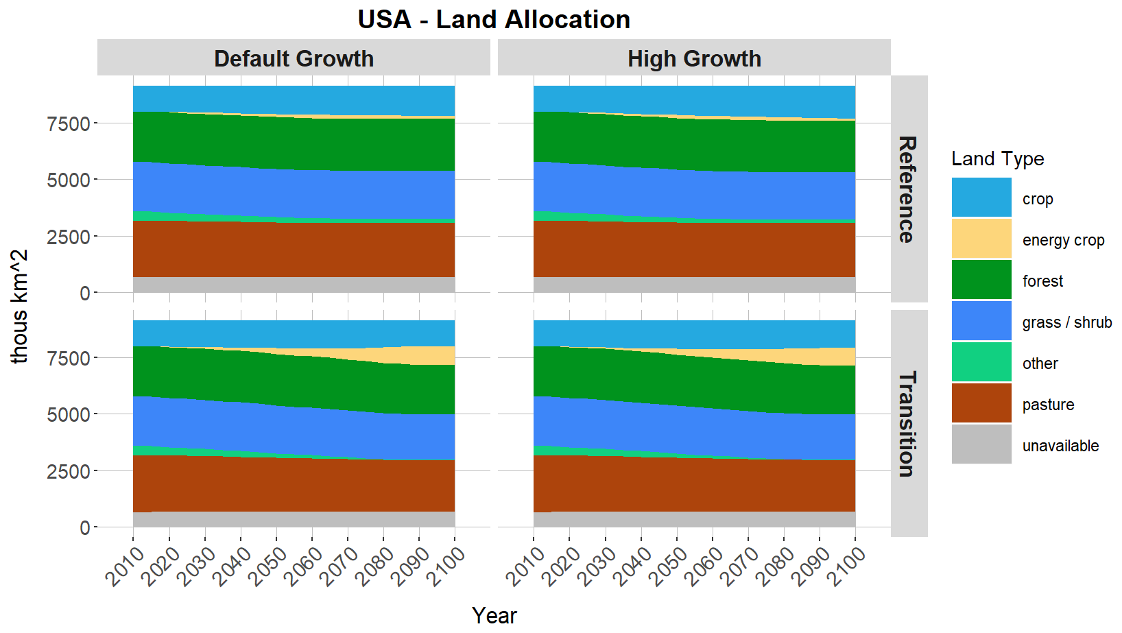
Figure 10 USA land allocation by aggregate land type and scenario. Columns reflect alternate assumptions about socioeconomic drivers; rows represent alternate assumptions about energy system evolution.

6.4 Land

GCAM-USA tracks land allocation in the USA across more than a dozen crop categories (corn, wheat, rice, other grains, fiber, root, sugar, and oil crops), two types of dedicated energy crops (trees and shrubs), managed and unmanaged forests, grasslands, shrublands, pasture lands, and several other land types. Figure 10 presents USA land allocation by aggregate land type for each scenario. In the Ref scenario, cropland expands gradually throughout the century, reaching 1.33 million square kilometers in 2100 (about 20 % higher than 2015 levels). Cropland expands less rapidly than irrigation water withdrawals, implying a shift to more water-intensive crops over time (the national share of irrigated agriculture is roughly constant throughout the scenario). A small amount of dedicated bioenergy cropland is also introduced throughout the century. This additional cropland comes mainly from pasture and other arable land; forest land expands marginally (2 % higher in 2100) in the Ref scenario. Cropland expansion is more significant in the High Growth scenario, with cropland reaching 1.43 million square kilometers in 2100. This additional cropland results in less allocation to most other land types, including energy crops, although the biggest differences (in absolute magnitude) are in other arable land and forests.

The Transition and High Growth + Transition scenarios, by contrast, entail initial cropland expansion followed by a contraction in the second half of the country, as traditional cropland is gradually replaced by energy cropland. Cropland in the Transition scenario is just 1.13 million square kilometers in 2100, just 1 % higher than 2015 levels; in the High Growth + Transition scenario, traditional cropland accounts for 1.21 million square kilometers in 2100, as a larger population demands more food. Thus, the Transition scenario has the largest energy cropland allocation at 814 000 km² in 2100 (42 % of total cropland), with the High Growth + Transition scenario next largest at 759 000 km² (39 %). It should be noted that this large bioenergy cropland expansion is driven by the fact that bioenergy is considered to be carbon-neutral in the energy system; the Transition and High Growth + Transition scenarios entail a long-term transition towards a lower-carbon energy system but do not include efforts to value or incentivize the sequestration of carbon in the land system. Both the Transition and High Growth + Transition scenarios entail lower forest, grassland, shrubland, pasture, and other arable land than the Ref and High Growth scenarios.

Figure 11 Percentage change in cropland allocation in 2100 relative to 2015 by water basin and scenario. Red shades indicate a reduction in cropland allocation, while blue shades indicate an increase in cropland.

As with other systems, the way these national trends unfold varies by region. Figure 11 presents the percentage change in cropland (excluding dedicated energy crops) in 2100 relative to 2015 by land region for each scenario. Bioenergy crops are excluded from Fig. 11 to emphasize the way food production shifts across basins within the scenarios. There is no dedicated bioenergy cropland in 2015 (the model base year and base year for the percentage changes in Fig. 11). Figure S6 presents absolute and percentage changes in traditional (food + feed) cropland, dedicated bioenergy cropland, and total cropland. In the discussion below, cropland refers to traditional (food + feed) cropland, excluding dedicated energy crops.

In the Ref scenario, every region (besides the Nelson River basin) has more cropland in 2100 than in 2015, with cropland increases ranging between 3 % to 113 % (national average: 18 %). The largest relative increases are in the southwestern US, with the Great Basin, Upper Colorado River, and Rio Grande basins all more than doubling cropland in 2100 (relative to 2015), although these basins currently have a relatively small amount of cropland (about 18 000 km² combined in 2015). The largest absolute increase by far occurs in the Missouri River basin, which adds nearly 70 000 km² of cropland over the century. These spatial trends are similar but larger in the High Growth scenario, with every basin increasing cropland and the Great Basin, Upper Colorado River, and Rio Grande basins seeing 132 %, 140 %, and 150 % increases in cropland in 2100 (relative to 2015), respectively.

The Transition and High Growth + Transition scenarios entail both increasing and decreasing cropland across basins. In the Transition scenario, 9 of 20 basins finish the century with less cropland than the final historical year; the biggest decrease is 29 000 km² in the Nelson River basin. The Missouri River basin again sees the largest increase in total cropland with 60 000 km² of cropland added by 2100; the largest relative increases are again in the Great Basin, Colorado River (Upper and Lower), and Rio Grande River basins. Finally, as mentioned above, while the Transition and High Growth + Transition scenarios both have less cropland than their reference energy system counterparts (due to increased demand for bioenergy crops), the High Growth + Transition scenario has more cropland because of greater population and corresponding total food demand. Thus, only 5 of 20 basins in this scenario experience net cropland contraction over the course of the century (and each is smaller than the corresponding reduction in the Transition scenario).

6.5 Comparison to historical data and other future scenarios

This section compares GCAM-USA v5.3_water_dispatch results to historical data and other future projections. Historical results for GCAM-USA are compared to inventory data for four metrics at the state level for the model's final historical year (2015). The four historical metrics are total final energy consumption (across all fuels and end-use sectors), total electricity generation (across all fuels), total water withdrawals (across all sectors), and energy system CO₂ emissions (excluding emissions from the land system). State-level final energy consumption comes from the Energy Information Administration's (EIA) State Energy Data System (SEDS) “All consumption estimates” data set (https://www.eia.gov/state/seds/sep_use/total/csv/use_all_btu.csv, last access: 1 October 2020). Historical data for electricity generation comes from the EIA's Electricity Data Browser (EIA, 2020a; https://www.eia.gov/electricity/data/browser/, last access: 22 January 2021). Data on state-level water withdrawals comes from the U.S. Geological Survey (USGS) (https://water.usgs.gov/watuse/data/, last access: 15 May 2020.), and data on historical CO₂ emissions by state is taken from EIA's Energy-Related CO₂ Emission Data Tables (https://www.eia.gov/environment/emissions/state/excel/table2.xlsx, last access: 22 January 2021).

GCAM-USA is initialized over five historical periods (1975, 1990, 2005, 2010, 2015) and calibrated (by estimating logit share weight parameter values) to match historical data (calibration is discussed in more detail below). For energy flows, land allocation, and agricultural production, an exact match is enforced in the historical period. Water use and CO₂ emissions are determined by coefficients calculated from historical data, but not forced to match observations. Historical observations are read into the model, which replicates these outcomes while maintaining GCAM's market equilibrium requirement that supplies and demands of all markets balance in each model period. Several data sets are used to provide historical calibration information for the model. At the global level, the IEA Energy Balances (IEA, 2019) is the primary data set used to calibrate historical energy flows, including energy production, transformation, and consumption. Fossil fuel production and consumption data are scaled globally to eliminate statistical differences and net stock changes and ensure supply–demand balance; electricity is similarly scaled for each GCAM region to remove inter-regional trade and statistical differences.

To ensure that global energy remains balanced, GCAM-USA downscales this processed IEA energy production, transformation, and consumption data for the USA using state-level shares derived from the EIA's State Energy Data System. Some sectors are disaggregated beyond the level of detail in core GCAM; for instance, the building sector includes additional building services and technological detail and utilizes the EIA's Residential Energy Consumption Survey (RECS) and Commercial Building Energy Consumption Survey (CBECS) to further disaggregate building energy. A full list of input data sets is included as Table S6; all model input data (except for the proprietary IEA Energy Balances data set) are available with the model or in the separate gcamdata package (https://github.com/JGCRI/gcamdata/, last access: 22 October 2021).

Within GCAM, each sector contains at least one subsector, which in turn contains at least one technology. Subsectors (often corresponding to competing fuels) compete for share of the sector's total output; technologies within a given subsector compete for share of the subsector's output. This competition occurs on the basis of relative costs using a probabilistic logit choice function, which assumes a distribution of realized costs due to heterogeneous real-world conditions and allocates market share on the probability that a technology has the lowest cost compared to competing options. GCAM's logit choice formulation is described in detail in Calvin et al. (2019). In short, technology shares within a nest are a function of the technology's cost, its share weight, the logit exponent, and the costs and share weights of other competing technologies in the nest. The exogenous logit exponent regulates the extent to which cost (or profit) dictates share; larger absolute logit exponent values lead to greater shares for the lowest cost (most profitable) technology when all else is equal. Technology costs in the logit equation include exogenous non-energy cost inputs, endogenous energy and water prices (combined with exogenous conversion efficiencies), and emissions or other policy costs; non-energy cost and efficiency assumptions reflect exogenous technological improvement for most technologies and sectors.

During the calibration routine, GCAM uses the cost of each subsector or technology to estimate the (unobserved) logit share weight parameters, ensuring that historically observed outcomes are reproduced (Calvin et al., 2019). Technology shares are derived from the historical (calibration) data, leaving share weights as the unknown parameter in the logit equation that is solved for. The share weight parameters capture unobserved factors, including preferences, which impact economic choice but are not explicitly represented in the model's choice indicator (cost). Share weights are typically held constant at their final (2015) calibration values or gradually converged to a common value in some future model period. Thus, the preferences captured by GCAM's calibration routine influence model decisions in future model periods (most strongly in initial model years). Table S7 provides an overview of how the calibrated share weights parameters for key sectors are applied in future model periods.

Figure 12 Comparison of state-level historical results (2015) from GCAM-USA to historical data for (a) final energy consumption, (b) electricity generation, (c) water withdrawals, and (d) energy system CO₂ emissions. The line in each figure is a one-to-one line indicating an exact match between historical data and model outcomes; the green band around this line corresponds to a ± 5 % deviation from historical data. Individual state results are indicated by the position of the corresponding state abbreviation. Note that the units and axis scales vary by panel.

Figure 12 presents a comparison of historical (2015) state-level results from GCAM-USA and the historical inventory data (described above) as a scatterplot, with historical data on the horizontal axis and GCAM-USA results on the vertical axis. The line in each figure is a one-to-one line indicating an exact match between historical data and model outcomes. As indicated by the tight grouping of data points along this one-to-one line, GCAM-USA results compare well to historical data for final energy consumption, electricity generation, and energy system CO₂ emissions.

Results for water withdrawals deviate more from the historical inventory data. This occurs for a couple of reasons. First, as discussed in Sect. 3.2.2, agriculture and land use is modeled at the land region level rather than the state level; water consumption from this sector is mapped to state level based on a 5-year running average share of withdrawals for each state-basin combination. The Huang et al. (2018) data used for this mapping runs only through 2010, and thus 2015 results are allocated to the states assuming 2010 shares. GCAM-USA also applies USA average irrigation efficiency values from Rohwer et al. (2007) to each land region; these values are likely to differ spatially, contributing to differences in state-level results compared to USGS data. A similar dynamic occurs with electric power sector withdrawals. Historical cooling system shares by state are based on data from 2012. While states are differentiated by the composition of cooling systems for each generation technology, water withdrawal (and consumption) demand coefficients for each power plant and cooling system combination are based on US national averages. Mining and livestock water withdrawals by state also diverge from USGS data somewhat, while municipal and manufacturing demands match historical data exactly.

Figure 13 Comparison of national energy system projections from GCAM-USA (red line) and nine scenarios from the EIA's 2020 Annual Energy Outlook (grey lines). Results for (a) primary energy consumption, (b) energy system CO₂ emissions, (c) electricity generation, and (d) electricity capacity.

Figure 13 compares the GCAM-USA Ref scenario to nine scenarios from the EIA's 2020 Annual Energy Outlook (AEO)¹. The AEO was chosen as the point of comparison for future results because it is one of the most cited projections of the future US energy system. The National Energy Modeling System (NEMS) is used to create the AEO projections. NEMS' geographic scope is limited to the USA; AEO results are mostly reported at the national level. Thus, the comparison in Fig. 13 focuses on national aggregate results, rather than subnational ones. Additionally, NEMS has strong detail in the energy system but does not represent the land and water systems; thus, the metrics compared in Fig. 13 – total primary energy consumption (across fuels), total energy system CO₂ emissions, total electricity generation, and total electricity capacity – focus on results from the energy system. Results are provided for the full future time horizon of each scenario (2020 through 2050 for the AEO and through 2100 for GCAM-USA).

Broadly, the GCAM-USA Ref scenario results fall within the range of AEO 2020 results for the scenarios shown through 2050. In terms of primary energy consumption, GCAM-USA's results for 2020 are about 10 % lower than AEO's Reference case. This is in part because AEO is calibrated to 2019 outcomes, while GCAM-USA's final historical year is 2015. By 2030, GCAM-USA is well within the range of primary energy consumption for AEO scenarios and remains there through 2050.

In terms of CO₂ emissions, GCAM-USA's simulated emissions in 2020 are 2 % lower than the AEO 2020 Reference case. From there, the models diverge. The GCAM-USA Reference scenario projects increasing CO₂ emissions through 2035, after which emissions decline for roughly 3 decades before rebounding to current (2020) levels in 2090. In contrast, AEO's scenarios generally project emissions decreasing to 2030 or 2040 before ticking up again thereafter. GCAM-USA's emissions growth is driven by increased emissions in the power sector, industry, and transport. Conversely, AEO projects decreasing emissions from electricity and transport, at least in part because the AEO “generally assumes that existing laws and regulations remain as enacted throughout the projection period” (EIA, 2020b), while the GCAM-USA Ref scenario does not explicitly include policies such as Corporate Average Fuel Economy (CAFE) standards or state-level renewable portfolio standards (RPS). By 2050, GCAM-USA Reference scenario CO₂ emissions are within the spread of AEO scenarios and almost identical to the AEO 2020 Reference case.

For the electric power sector, GCAM-USA and AEO are generally in good agreement about the size of the sector, both in terms of capacity and total generation. GCAM-USA anticipates higher electricity generation than the AEO 2020 Reference case over the next 4 decades, although it is always within the range of AEO 2020 cases. The GCAM-USA Ref scenario simulates slightly lower capacity than the AEO 2020 Reference case in the near-term, but falls right in the middle of the AEO 2020 range in the longer-term.

7 Discussion and conclusions

GCAM-USA has been used by public (The White House, 2016) and private (Lempert; et al., 2019) sector decision-makers and the research community (Feijoo et al., 2018; Iyer et al., 2019) to understand interconnections and trade-offs between US economic, energy, agriculture, land, and water systems in a global context. The latest version of GCAM-USA, described here, includes several important new features that open the possibility for new avenues of research in subnational energy–water–land interactions, such as the impact of water constraints on electricity capacity expansion (e.g., Liu et al., 2019); the impacts of agriculture and electricity production on virtual water trade within the US (e.g., Graham et al., 2020); implications for electricity and end-use sectors of increasing deployment of variable renewable energy technologies; or energy–water–land implications of higher renewable fuel standard targets in the US. It also demonstrates how subnational and sub-annual detail can be incorporated in a global multi-sector modeling framework, serving as a blueprint for other regionally detailed models like GCAM-China (see, for example, Cui et al.,  2021).

With models like GCAM-USA, there is a constant balancing act between global and sectoral coverage; regional, temporal, and process resolution; and computational tractability. While GCAM-USA has advanced significantly in recent years, there are still many areas ripe for model development, including the following examples.

1. State-level resource endowments and production, particularly for fossil resources (oil, gas, coal) but also hydropower as state-level fossil resource endowments and production would permit the accounting of associated energy and emissions inputs at the state level and facilitate the exploration of changes in regional patterns of resource production under alternate future scenarios. While hydropower production is exogenously prescribed for each state and model period (hydropower capacity and capacity factors are fixed at 2019 levels for all future periods), hydropower capacity and generation could vary in the future under different socioeconomic, technology, policy, or water-availability scenarios, which could play out differentially among the states and impact the generation and final energy mix for a given state and its electricity trade partners.

2. Improved representation of electricity storage, electricity trade, and electrification potential of end uses (particularly industry and transportation).

3. Improved representation of infrastructure, including electricity transmission lines, oil and gas pipelines, and water conveyance network.

4. Increased detail in the industrial sector, representing different industrial subsectors and their corresponding technologies.

5. Improved representation of existing policies in the GCAM-USA Reference scenario, including federal policies (e.g., CAFE standards) and state-level policies (e.g., Hultman et al., 2020).

6. Complete representation of non-CO₂ emissions because GCAM-USA currently does not represent non-CO₂ emissions for energy activities modeled at the state-level. Without emissions of these species in the USA, the picture of radiative forcing agents in the atmosphere is incomplete; thus, the Hector climate model is disabled when running GCAM-USA, and climate outcomes are not available for GCAM-USA scenarios. Complete accounting of non-CO₂ emissions (both non-CO₂ greenhouse gases and traditional air pollutants) is an ongoing development priority for GCAM-USA; studies have been published with research versions of the model containing such capabilities (Feijoo et al., 2020; Ou et al., 2020; Shi et al.,  2017).

7. State-level drivers for all activities because while decisions and outcomes in the land system are modeled at the subnational level, these decisions are driven by national aggregate socioeconomic drivers which determine demands for food, fiber, and other agricultural products, rather than heterogenous state-level demands, preferences, and economic and policy contexts. Some energy transformation processes (e.g., gas processing, hydrogen production) also remain nationally resolved.

Ultimately, there are trade-offs between model detail on the one hand and computational tractability on the other. As presently configured, GCAM-USA requires balancing supplies and demands for nearly 1700 markets simultaneously and produces databases in excess of 2 GB per scenario (run to 2100). The model can presently be run on a personal computer with 8 GB of RAM; additional developments inevitably increase memory requirements, solution complexity, and database size, although great effort is invested in making the GCAM framework as computationally efficient as possible to strike a balance between cutting-edge scientific capability and user functionality.