the Creative Commons Attribution 4.0 License.
the Creative Commons Attribution 4.0 License.
 | 21 Mar 2022
Flow-Py v1.0: a customizable, open-source simulation tool to estimate runout and intensity of gravitational mass flows
Christopher J. L. D'Amboise
Michael Neuhauser
Michaela Teich
Andreas Huber
Andreas Kofler
Frank Perzl
Reinhard Fromm
Karl Kleemayr
Jan-Thomas Fischer
Models and simulation tools for gravitational mass flows (GMFs) such as snow avalanches, rockfall, landslides, and debris flows are important for research, education, and practice. In addition to basic simulations and classic applications (e.g., hazard zone mapping), the importance and adaptability of GMF simulation tools for new and advanced applications (e.g., automatic classification of terrain susceptible for GMF initiation or identification of forests with a protective function) are currently driving model developments.
In principle, two types of modeling approaches exist: process-based physically motivated and data-based empirically motivated models. The choice for one or the other modeling approach depends on the addressed question, the availability of input data, the required accuracy of the simulation output, and the applied spatial scale. Here we present the computationally inexpensive open-source GMF simulation tool Flow-Py. Flow-Py's model equations are implemented via the Python computer language and based on geometrical relations motivated by the classical data-based runout angle concepts and path routing in three-dimensional terrain. That is, Flow-Py employs a data-based modeling approach to identify process areas and corresponding intensities of GMFs by combining models for routing and stopping, which depend on local terrain and prior movement. The only required input data are a digital elevation model, the positions of starting zones, and a minimum of four model parameters.
In addition to the major advantage that the open-source code is freely available for further model development, we illustrate and discuss Flow-Py's key advancements and simulation performance by means of three computational experiments.
-
Implementation and validation. We provide a well-organized and easily adaptable solver and present its application to GMFs on generic topographies.
-
Performance. Flow-Py's performance and low computation time are demonstrated by applying the simulation tool to a case study of snow avalanche modeling on a regional scale.
-
Modularity and expandability. The modular and adaptive Flow-Py development environment allows access to spatial information easily and consistently, which enables, e.g., back-tracking of GMF paths that interact with obstacles to their starting zones.
The aim of this contribution is to enable the reader to reproduce and understand the basic concepts of GMF modeling at the level of (1) derivation of model equations and (2) their implementation in the Flow-Py code. Therefore, Flow-Py is an educational, innovative GMF simulation tool that can be applied for basic simulations but also for more sophisticated and custom applications such as identifying forests with a protective function or quantifying effects of forests on snow avalanches, rockfall, landslides, and debris flows.
- Article
(5749 KB) - Full-text XML
- BibTeX
- EndNote


The term gravitational mass flow (GMF) covers various natural hazard processes such as snow avalanches, rockfall, landslides, and debris flows. GMFs are characterized by (1) the composition of their mass and (2) the behavior of their motion (Köhler et al., 2018; Okuda, 1991; Varnes, 1978). However, certain commonalities are shared between most GMFs such as the fact that their motion is driven by the force of gravity and that they are all processes acting on hillslopes (Varnes, 1978).
GMF simulation tools are crucial for developing natural hazard zoning maps and integrated natural hazard risk management (Corominas et al., 2014; Fressard et al., 2014; Guillard and Zezere, 2012; Barbolini et al., 2011; Dorren et al., 2011; Fell et al., 2008; Sauermoser, 2006; Van Westen et al., 2006; Crozier and Glade, 2005; Dorren, 2003; Guzzetti et al., 2002). To optimize risk mitigation measures, e.g., by installing technical protection measures or planning and implementing nature-based solutions and avoidance strategies efficiently, GMF runout models can be used in economic studies (Moos et al., 2018; Teich and Bebi, 2009; Fuchs et al., 2007).
Many GMF-specific models exist, which provide estimations of runout lengths for snow avalanches (Christen et al., 2010; Sampl and Granig, 2009; Christen et al., 2002; McClung and Lied, 1987; Bakkehøi et al., 1983; Lied and Bakkehøi, 1980), landslides (Brenning, 2005), or rockfall (Dorren, 2012; Guzzetti et al., 2002). More general GMF models can be applied to various GMFs and are either process-based physically (Wirbel et al., 2021; Mergili et al., 2017; Christen et al., 2010; Sampl and Zwinger, 2004) or data-based empirically motivated (Horton et al., 2013). The main differences between these two types are the larger number of input parameters and expensive computational resources required for process-based physically motivated GMF models (hereafter referred to as process-based models) in contrast to data-based empirically motivated models (hereafter referred to as data-based models) that usually involve fewer input parameters and are computationally inexpensive; however, process-based models provide more detailed information about a GMF process and its interactions with the terrain and obstacles in the flow path. The choice for one or the other modeling approach depends on the addressed question, the availability of input data, the required accuracy of the simulation output, and the applied spatial scale.
Depending on their application, one can choose between those two types of modeling approaches: process-based models are suitable for most applications provided that their input data requirements are met; however, obtaining detailed parameter sets over large areas is labor-intensive and often not possible. Therefore, process-based models are best used on smaller (hillslope) scales and in data-rich domains (Corominas et al., 2014; Van Westen et al., 2008), but methods to overcome the lack of parameterizations have even been developed to tackle back calculations by solving the inverse problem (Fischer et al., 2015; Eckert et al., 2010; Ancey et al., 2003). In recent years, a number of data-based models, which require fewer input parameters, have been developed and applied to regional-scale case studies and for various GMFs. For example, random-walk-based models have already been applied to debris flows and other GMFs (Mergili et al., 2015; Gamma, 1999). Huggel et al. (2003) developed a similar flow-routing model and used it to assess GMFs related to glacier lake outbursts, but their model can also be applied to other GMF types such as ice–rock avalanches (Huggel et al., 2007; Noetzli et al., 2006). Horton et al. (2013) published the Flow-R simulation tool, which primarily aims at regionally assessing debris flow susceptibilities, but is also applicable to other processes and variable friction relations. While data-based models mostly lack a physical interpretation of their results, they are computationally inexpensive and require fewer input data. In addition, data-based and process-based approaches can be combined in one model (Barbolini et al., 2011; Scheidl and Rickenmann, 2011). Using a combination of observations, data-based models, and process-based models for hazard zone mapping has been proposed to overcome the lack of hard-to-measure parameterizations for process-based models, especially for statistically sensitive variables (Barbolini et al., 2000).
We present the innovative and educational Flow-Py simulation tool, which employs a data-based motivated approach to predict the magnitude, i.e., runout (spatial extent including starting, transit, and runout zones) and intensity (effects of a GMF at a specific location), of GMF processes. Flow-Py builds on the ideas and algorithms from existing data-based GMF models. The Flow-Py algorithm is based on a flow path identification in three-dimensional terrain (routing) and concepts for runout and intensity estimates along this path (stopping). To determine the GMF's runout and intensity we utilized well-known runout (travel) angle concepts (Heim, 1932) and derived corresponding geometrical quantities to motivate the Flow-Py model equations. These geometric relations serve further as a reference to validate the Flow-Py implementation and results. In addition to runout and intensity predictions, Flow-Py simulation results are also a measure of how exposed a location in the flow path is regarding the number of starting zones and associated transit zones, which route flux through that location.
This contribution is structured as follows: in Sect. 2 we describe the motivation and implementation of our GMF model, which is further explained in the code repository (Neuhauser et al., 2021). A validation experiment is presented in Sect. 3, which shows simulation results from three simple generic slopes. The performance of Flow-Py is tested via a regional-scale simulation of snow avalanches in Sect. 4. The customization of Flow-Py is described in Sect. 5 and shows how flexible the simulation tool is and that it can be easily adapted with extensions to specific modeling questions.
With this contribution we enable the reader to reproduce and understand the basic GMF model concepts and their implementation in the Flow-Py code.
The main objectives of the Flow-Py simulation tool are to compute the spatial extent (hereafter referred to as runout) of GMFs, which consists of starting, transit, and runout zones, and the intensity of the GMF. Flow-Py is based on data-driven empirical modeling ideas (Heim, 1932) with automated path identification (Holmgren, 1994; Horton et al., 2013; Huber et al., 2016; Wichmann, 2017) to solve the routing and stopping of GMFs in three-dimensional terrain. Data-based models often require fewer input data as well as a less complex parameterization and solution (e.g., no time-dependent equations are usually solved), than process-based models. The Flow-Py simulation tool has been designed as a computationally inexpensive data-based model, which facilitates its application on regional scales, including a large number of GMF paths. Simulations of single starting cells take 1 to 10 s, whereas process-based, depth average simulations usually operate on the order of minutes. This can be attributed to the fact that no time-dependent equations, which process-based models are built on, are solved in the underlying model equations of Flow-Py. The Flow-Py code is written in the Python computer language, taking advantage of Python's object-oriented class method. The well-structured model implementation allows users to address GMF-specific modeling questions by keeping the parameterization flexible and enabling inclusion of customized model extensions and add-ons. Flow-Py has already been applied to dry snow avalanches, rockfall, and shallow-seated landslides by adapting the parameterization. Experience from similar studies also suggests that the model may also be suitable for other GMFs such as debris flows and wet snow avalanches (Holmgren, 1994; Gamma, 1999).
The development philosophy to maximize the applicability of Flow-Py builds on the following:
-
flexible yet minimal input data requirements,
-
simple parameterizations which can describe a range of GMFs, and
-
a highly adaptable and customizable source code.
In the following sections the model motivation, implementation, input data and Flow-Py results, and underlying model equations are explained in detail.
2.1 Model motivation
Flow-Py's routing and flow path identification in three-dimensional terrain were inspired by the gravitational process path model CPP (Wichmann, 2017), which introduced a weighting factor for the flow direction, and the programming architecture and persistence equations of Flow-R (Horton et al., 2013), combined with an adapted version of the flow direction algorithm (Holmgren, 1994), to appropriately model movement in flat and uphill terrain. The routing is based on local terrain and prior movement (flow direction and process intensity), which determines the flow path from starting to transit and runout zones and simultaneously describes the flow concentration, including lateral spreading. To estimate the process intensity along the identified path and the runout by introducing a stopping criterion we utilize the well-known runout angle (α) concept (Heim, 1932; Lied and Bakkehøi, 1980; Bakkehøi et al., 1983; Körner, 1980) and derived corresponding geometrical quantities to motivate the Flow-Py model equations. Figure 1 depicts the runout angle along with the corresponding geometric relations in a two-dimensional representation along a GMF path, building the foundation for the underlying model equations.

Figure 1GMF path with altitude z(s), projected travel distance s, and local slope angle ψ with starting point s0,z(s0) and runout point sα,z(sα). The corresponding geometric quantities are directly related to the runout angle α concept and include the local travel angle γ, with corresponding total altitude change zγ and the process intensity measure zδ with angle δ.
The geometric relations are directly deduced from the runout angle α and allow us to motivate the stopping and intensity estimates. Additionally, the geometric solution, represented by the α line from starting (s0,z(s0)) to the runout (sα,z(sα)) points, serves as a reference for a model validation. Important quantities include the local travel angle γ,
which, at the end of the GMF path, corresponds to the total travel angle (i.e., the so-called runout angle α; Heim, 1932) that can be expressed as
The local travel angle height zγ corresponds geometrically to the total elevation drop zγ from the starting point s0 to the currently projected runout length s along the path:
The total elevation drop zγ splits into zα,
which is associated with the dissipation kinetic energy height, and zδ,
which is a measure of the process intensity corresponding to the kinetic energy height (based on the principles of energy conservation, assuming a block movement with frictional dissipation associated with a Coulomb friction; Heim, 1932).
2.2 Implementation
The Flow-Py simulation tool is implemented based on object-oriented programming ideas, which allows for easy model customization (Neuhauser et al., 2021). Flow-Py is written in the freely available modern programming language Python3 (Van Rossum and Drake, 2009), which is widely used and supported by an active online community. The simulation tool is highly adaptable, and different routing and stopping routines can be easily implemented, which enables the user to adjust the parameterization, also for multi-model runs and the equations that govern the movement of the mass downslope as well as to implement Flow-Py in model chains. Flow-Py can be run either by command line allowing it to be called by external programs or in a BASH file, or with a simple GUI, which guides the user through choosing input files and the parameterization.
A GMF usually has one or more starting zones that span over a single cell or multiple starting cells. Flow-Py computes the so-called path, which we define as the spatial extent of the routing from each starting cell to the stopping cells. Each starting zone is associated with its own unique path; however, a certain location in the terrain can belong to many paths. Flow-Py identifies the path with spatial iterations on the cell level, starting with a single cell of a starting zone and then transferring the final results of the cell and path levels to the output raster level (see Fig. 2). To route on the three-dimensional terrain operating on a quadrilateral grid, we implemented the geometric concepts that have been introduced in Sect. 2.1. That is, each path calculation starts with a starting cell, operating on the cell level, requiring the definition of parent, base, child, and other neighbor cells (see Fig. 2). For the discretized model equations that operate on the cell level we use capital letters to distinguish the variables from the geometric motivation equations (see Sect. 2.1), with superscripts for the specification and subscripts for the cell indices.
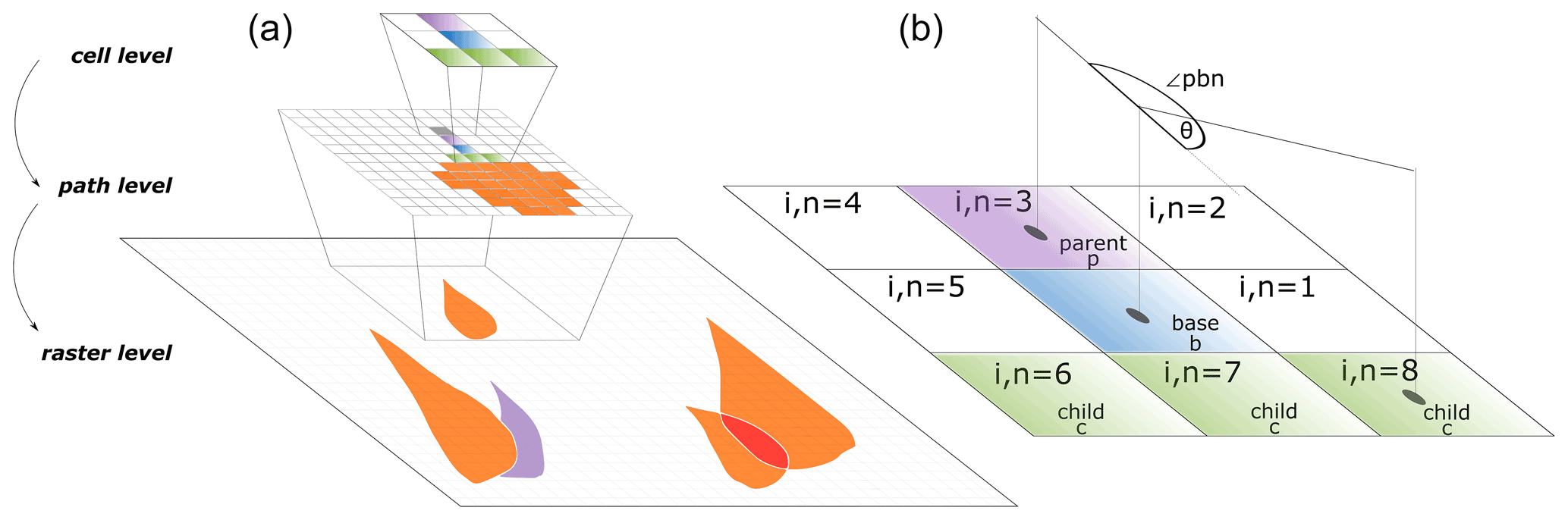
Figure 2(a) The raster level summarizes the simulation results and output quantities for all GMF paths. The path level is the spatial level that contains the spatial extent of a path associated with one starting cell. (b) Iterative routing is done on the cell level. During an iteration the cells are defined as parent p, base b, child c, and all neighbor cells get two indices i and n. The angle θ is the deviation between the projected incoming and outgoing directions, with the angle ∠pbn formed from the directions of parent p to base b and from base b to neighbor n cells.
The Python class object developed for Flow-Py is called Flow-Class, which can store values and functions. A Flow-Class is created for each cell that is part of one path when the neighbor cell is recognized as a child cell and is then added to the calculation queue. The Flow-Class saves information about a single cell, such as location, its parent cell(s), the output quantities, and other information needed for further calculations or computing the output raster. The cells in the calculation queue will be the base cell (center cell) for subsequent calculations. Information on the iteration step is temporally stored to the respective cell's Flow-Class. When the path calculations are finished, values from each cell's Flow-Class are updated to their respective location in the result array such that either a maximum value (e.g., , the maximum Zδ for a cell over all path calculations) or a running sum (e.g., , the sum of all Zδ values for a cell over all path calculations) of all calculated paths that route flux through that cell is stored. The Flow-Class can be extended to store additional information that can be used to adjust stopping and routing calculations; e.g., the runout angle α is saved in the Flow-Class and could be adapted and scaled with to account for an energy-dependent friction.
Using Python's object-oriented class method is a major advantage for advanced users since they can easily develop custom extensions or add-ons. We present an example for a back-tracking extension, which saves information of infrastructure located in GMF flow paths in the Flow-Class adapting the Flow-Py output in Sect. 5.
2.3 Input data
Flow-Py's core function loads and handles all input data, which are a digital elevation model (DEM) and a release raster in .asc or .tiff format. The release raster shows observed or potential GMF starting zones containing one or several starting cells. The release raster can be created by vector-to-raster conversion of polygon mappings by expert or by onset-susceptibility modeling. Flow-Py employs parallel processing for short model run times by splitting the release raster and DEM into tiles. Each tile is solved independently and sequentially in its own dedicated computer core and processing threads. Multi-processing is set as the Flow-Py default; i.e., the number of free cores and the amount of RAM are first checked before splitting the starting cells and spreading runout calculations among the free computer cores, making sure that the amount of RAM is not exceeded. The individual calculations are merged by updating the result arrays, which are transformed into an output raster.
The release raster shows potential GMF starting zones containing one or several starting cells. The DEM and the release raster must be in the same extent and resolution with no resolution limit; however, 5 and 10 m raster resolutions have been tested. The major differences between different types of GMFs in regional runout modeling is the behavior of the movement and its runout, which can be summarized by the runout length and the convergence or divergence of the spreading movement. These behaviors are controlled by the parameterization of the stopping and routing routines in Flow-Py.
2.4 Model equations and path identification
The Flow-Py model equations are formulated with respect to an equidistant quadratic grid with the same resolution and extent as the input raster.
During each spatial iteration, calculations are made on a 3×3 cell subset of the raster, for which the flux across the base cell (subscript b) is solved (see Fig. 2). The eight neighbor cells to the base cell (subscript i and n) can be parent cells (subscript p) during an iteration step acting as flux source cells or child cells (subscript c) acting as flux sink cells.
The governing runout modeling question is broken down into two subquestions.
-
Where does the GMF move to?
-
Where does the GMF stop?
These questions are addressed in two dedicated modeling routines called the routing routine and the stopping routine.
2.4.1 Routing
The routing routine considers a terrain contribution Ti and a contribution accounting for prior motion called persistence Pi (Horton et al., 2013); the flux is solved from parent cells through the base cell to child cells. Equation (6) is the basis of the routing algorithm and shows how the terrain contribution Ti and the persistence contribution Pi are combined to distribute the routing flux:
Ri is the routing flux from the base cell to neighbor cell i and Rb is the total routing flux into the base cell (for starting cells ). To conserve Ri, the amount of Rb must be equal to Ri unless a stopping criterion is met (see Sect. 2.4.4). To conserve flux, Ti and Pi to cell i are normalized across all neighboring cells n. The normalized direction is then scaled with Rb.
2.4.2 Terrain-based routing
The terrain-based routing accounts for the guiding effect of the slope on the movement. To distribute the flux we utilize the terrain-routing function:
where Ti is the normalized terrain-based routing from the base cell i and is the distribution angle with the local slope angle ψi from the center point of the base cell b to the center points of neighbor cells i where positive slopes indicate a downhill direction. The distribution function tan ψi is used as a weight to give preference to distributing flux to steeper slopes; this distribution function allows for routing on flat and uphill terrain by returning values <0 for . The distribution function reaches a maximum at , which is a vertical drop or free fall, and a minimum at , where tan ψi≈0 occurs at a vertical rise or wall face.
To control the concentration of routing flux an approach based on the multiple flow direction algorithm for runoff has been employed (Holmgren, 1994). The exponent exp, together with the flux cutoff (see Sect. 2.4.6), controls the lateral spreading of the flow (Horton et al., 2013). When exp increases, the terrain-based routing flux is concentrated to the steepest decent. Together with the flux cutoff >0, this results in the path's lateral spreading being reduced. As exp→∞ the divergence results in a single flow direction (block movement) and as exp→1 wide spreading is encouraged (fluvial movement). However, other terrain-based routing approaches can be easily implemented in Flow-Py (see Horton et al., 2013, for a summary).
2.4.3 Persistence-based routing
The persistence-based routing contribution aims to account for the influence or prior GMF movement on the subsequent routing. It must be noted that persistence is empirically derived and may be conceptually comparable to momentum; however, Flow-Py's underlying model equations do not account for mass (and hence momentum).
Equation (8) shows the persistence routing function Pi for neighbor cell i:
which consists of two components, the direction Dn in Eq. (9) and the intensity , which has classically been called energy line height (Körner, 1980). Because a base cell can receive flux from many parent cells p the persistence routing function is calculated over all neighbor cells n considering the incoming flux from each parent cell.
The direction Dn maintains the flow direction from a parent cell (p, flux source) to the base cell b. Weights are used to define the flow direction and are expressed as
where is the resulting deviation angle between the projected incoming and outgoing direction, with ∠pbn as the angle formed from the directions of parent cell p to base cell b and from base cell b to neighbor cell n (compare to Fig. 2). Cells located opposite a parent cell are assigned the full weight of 1, whereas cells 45∘ off the direct flow direction get a weight of cos (45∘) or 0.707, similar to Horton et al. (2013).
The reason that the persistence function passes flux through three cells and not only one is to compensate for the restriction that there are only eight directions to move on a raster grid. A weight of 0 is given to all other cells including the parent cell.
The intensity is stored in the Flow-Class of the parent cell p from a previous iteration step, and the value of Zδ is saved in the Flow-Class of each child cell. If one child cell has more than one parent cell, then (maximum value of Zδ for the many combinations of routes to a cell on a single path) is stored in its Flow-Class.
The intensity at the neighbor cell n is calculated cell-wise, i.e., cell to cell throughout the spatial iterations. The intensity refers to the iterative part of that is associated with the spatial step from the base cell b to the neighbor cell n. Equation (10) shows the calculation of , where is the intensity of the base cell b, which is stored in its Flow-Class. was calculated on a previous spatial iteration when the current base cell was a child cell:
where is calculated with respect to
where the subscript bn refers to base cell b to neighbor cell n, with the distance Sbn and the iterative energy quantities , and (see Fig. 1).
The total projected distance along the GMF path Sn is expressed as
The parent cell further away from the stopping condition (larger Zδ) will have more influence on the routing flux. After all n parent cells are calculated for each neighbor i the persistence-based routing Pi is combined with the terrain-based routing Ti, as seen in Eq. (7). When the parent cell has a large the persistence-based routing Pi will be the dominant term in Eq. (7); however, if is small, then the terrain-based routing Ti will dominate the routing direction.
There are two limits that are imposed in the persistence routing routine: first, any cell that has previously been a base cell cannot be a child cell (a parent cell cannot be a child cell). The disadvantage of this limit is exerted on half-pipe-shaped terrain in which the mass moves up a slope and back down on the same path but in the opposite direction. This limit is necessary to keep small amounts of flux from routing back and forth in terrain shaped like a bowl. The major advantage of this limit is the reduction of iteration steps by not calculating further flux for child cells resulting from flux oscillating in a bowl feature.
The second limit is imposed on the maximum value of , which is a limit of the process intensity () corresponding to a kinetic energy height or GMF velocity limit, respectively:
which is important for some GMF types because it is analogous to introducing a turbulent friction coefficient in a process-based model (Horton et al., 2013). In the examples used in Sects. 3, 4, and 5, no such limits are imposed.
2.4.4 Stopping
Two stopping criteria are employed: the first is a runout angle criterion that limits how far the GMF runout goes. The second is a flux cutoff stopping routine, which, together with the divergence control (exp) in the routing routine, limits the lateral spreading of the path. The GMF will not propagate further if either stopping criteria is met; however, the runout angle mainly determines the total travel distance in the main flow direction, while the flux cutoff influences the lateral spreading.
2.4.5 Runout-angle-induced stopping
The runout-angle-induced stopping routine is based on the geometric quantities derived with the α angle concepts (see Eqs. 1 to 5; see Fig. 1). The local travel angle γn is the inclination of the line formed from the top of the starting zone to the current neighbor cell n.
The stopping condition is reached when γn<α, i.e., when
When the stopping condition is met, no child cells are assigned in the next iteration step.
2.4.6 Routing-flux-induced stopping
The second stopping criterion is based on the assumption that a GMF must have a critical amount of routing flux Ri to continue its propagation. If the GMF has an excessively divergent flow concentration that dilutes down and across a slope, then the flow concentration (that can be associated with GMF mass) disappears at a critical amount of spreading corresponding to the critical routing flux threshold Rstop.
The routing flux stopping criterion is met when
the runout angle stopping condition is also met, and neighbor cell i is not a child cell. If Ri≥Rstop and the runout angle stopping condition is not met, then neighbor cell i is a potential child cell and is added to the calculation queue, and a Flow-Class is accepted.
The routing-flux-induced stopping mainly limits the width or spreading of the path. The magnitude of the routing flux of the potential child cell Ri relates to the percentage of initial routing flux from the start cell, where the starting flux Rstart=1. As a default, has been adopted in Flow-Py and is shown in the examples in Sects. 3, 4, and 5.
2.5 Flow-Py outputs
The outputs of Flow-Py are a set of rasters in the same resolution and extent as the input DEM, providing information about the runout of the GMF and different measures of the intensity.
-
is the local maximum Zδ for a cell over all path calculations. This is a geometric measure of highest intensity in terms of Zδ for all starting cells, which can be associated with the maximum kinetic energy that is expected at each location (raster cell).
-
Rmax is the local maximum routing flux for a cell over all path calculations. This is a measure of intensity in terms of the maximum of flow concentration from a single start cell that is expected at each location (raster cell).
-
is the sum of all Zδ for a cell over all path calculations. This is a measure of intensity in terms of Zδ combined with the number of starting cells that route flux through a location (raster cell).
-
CC is path cell counts, which is the number of paths that route flux through a location (raster cell). Together with an average of Zδ can be formed.
-
γmax is the local maximum flow path travel angle for a cell over all path calculations. This is a measure of how exposed a location is with regards to how close the highest GMF intensity in terms of Zδ is to the runout angle stopping criteria.
This first computational experiment demonstrates the Flow-Py routing and stopping algorithms for GMF modeling on simple but increasingly complex generic topographies. We highlight how GMFs interact with different terrain features and show the influence of different parameterizations on the flux; however, we do not perform a detailed parameter study, which is beyond the scope of this contribution. First, we describe the scenarios (terrain and model parameterizations) and present the simulations results. For each scenario, we altered the model parameterization or terrain complexity. Then the behavior of the simulations and a comparison to the geometrically expected results, which allows for validation of the model implementation, are summarized and discussed.
The generic topographies used for Flow-Py testing were generated using the “generate topography” functions provided within AvaFrame (Wirbel et al., 2021). Terrain data were saved in ASCII raster format (.asc) with 10 m resolution. The release raster consisted of three 100 m2 neighboring starting cells (starting zone = 300 m2, 3 raster cells) located close to the top of the generic terrain model at an elevation of 982 m. The three starting cells are centered on the y plane.
3.1 Parabolic, open slope
The first example topography is built from a parabolic slope that connects with a flat (0∘ slope) plane. The extent of the terrain model is 5000 m (x axis) by 1500 m (y axis). The transition from parabolic slope to flat plane takes place at 2250 m along the x axis. The total altitude difference of the terrain is 1000 m, with a maximum altitude located at x=0. This parabolic slope example is used as the base topography, to which more complex terrain features are added.
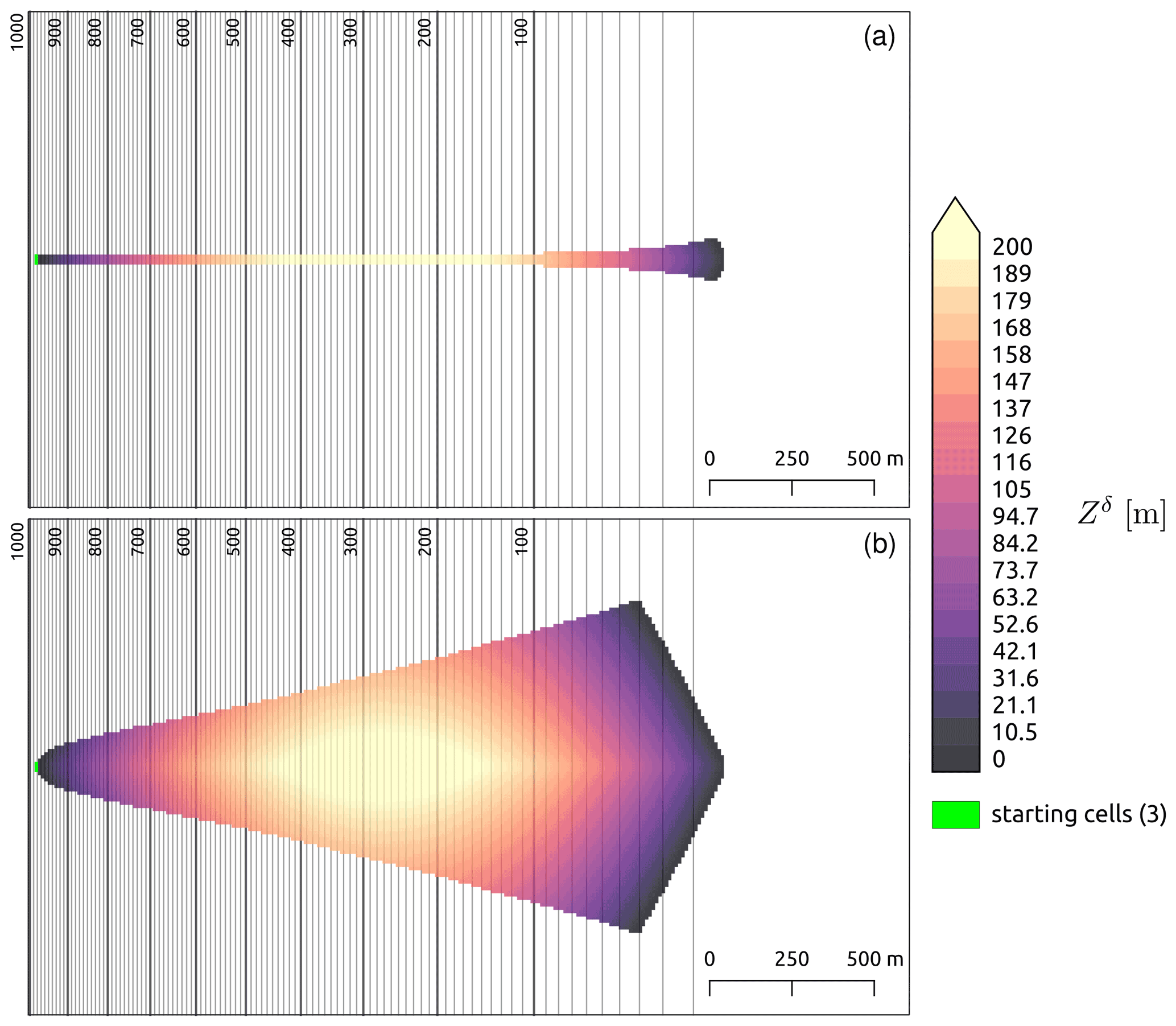
Figure 3GMF runout modeled with Flow-Py on a simple parabolic slope connected to a flat plane with the runout angle . The divergence control is exemplified with a low spreading (a, exp=100) and a high spreading (b, exp=8) simulation. Both examples use a flux cutoff of and m (the height of Mount Everest, i.e., no effective limit is used). Cooler colors indicate areas where the process has a relatively low intensity with regards to , and warmer colors show areas where the process has a relatively high intensity with regards to , which is associated with maximum kinetic energy.
Figure 3 shows the parabolic slope and the results from two simulations, for which the color scale is the as an indication of the intensity of the GMF. The parameterizations used for these simulations are , , and m (the height of Mount Everest, i.e., no effective limit is used). The parameter that controls the concentration of flux (exp) is varied between the two simulations to show results with low spreading (Fig. 3a, exp=100) and high spreading (Fig. 3b, exp=8). The run time for these examples when run on a personal computer with an eight-core processor (AMD Ryzen 7 2700X eight-core Processor 3.70 GHz) and 32 GB RAM is 1 s for the low spreading case (Fig. 3a) and 16 s for the high spreading case (Fig. 3b).
Comparing the top and bottom panels of Fig. 3, it can be seen that keeping the terrain, the runout angle, and Rstop the same but reducing the exp value increases the spreading of the GMF, yet the runout length does not change. In the low spreading example in Fig. 3a (exp=100), the behavior of the downhill flow is restricted to a single flow direction in steeper terrain. Once the slope flattens out the path diverges with very limited spreading. The small amount of spreading in flatter terrain can be explained by the low , which results from the persistence-based routing being dominated by the terrain-based routing. The front of the GMF runout is defined by the runout-angle-induced stopping routine with (black). The sides of the GMF process path are defined by the routing-flux-induced stopping routine, and because the runout-angle-induced stopping condition is not met.
3.2 Parabolic, channelized slope
This topography has the same extent, centerline profile, and configuration as the parabolic slope in Sect. 3.1; however, an hourglass-shaped channel is added, which begins wide and becomes narrow, returning to a wide channel in the runout zone again. The parameterizations used for this scenario are , exp=8, , and m such that one can compare it to the simulation results shown in Fig. 3b.

Figure 4GMF runout modeled with Flow-Py on a parabolic slope with a channel with , exp=8, , and m. The colors show the value of , which is associated with maximum kinetic energy. The topography is a simple parabolic slope connected to a flat plane.
This example highlights the routing-flux-induced stopping and the terrain-based routing (Fig. 4). The GMF travels down the channel and does not spread like in the previous example (Fig. 3). That is, the routing algorithms acts on the channelized terrain and concentrates the flux in the center of the channel. The GMF does not spread outside the channel because the flux that is routed up the channel walls does not exceed the flux cutoff Rstop, and hence the routing-flux-induced stopping criterion is met.
3.3 Parabolic, channelized slope with superimposed dam
The topography used in this scenario is the same as in the last section (Sect. 3.2) including a superimposed obstacle that crosses the terrain such that the GMF must travel uphill to overcome it. We refer to this obstacle as a dam as it could resemble a dam built in the GMF path. This example highlights how the Flow-Py simulation responds to flat or uphill terrain, which is where persistence-based routing will dominate over the terrain-based routing. The parameterizations used are , exp=8, , and m so that the result can be directly compared with the spreading example shown in Fig. 3b and the channelized example (Fig. 4). The dam has the shape of a Gaussian function with a width of 75 m and a height of 75 m, which is added on top of the topography of the parabolic slope with a channel. The center of the dam (maximum height) is located at 1350 m (Fig. 5).
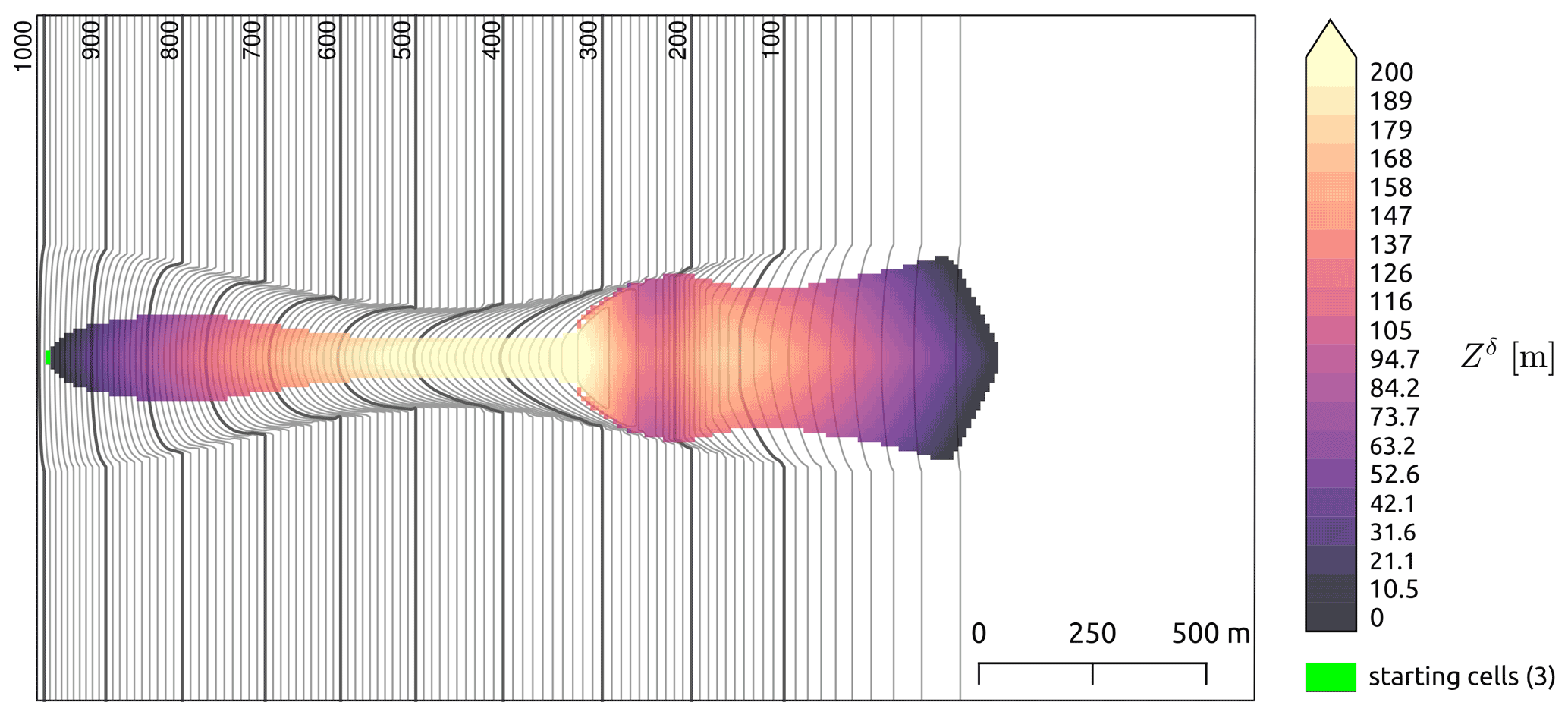
Figure 5GMF runout modeled with Flow-Py on a parabolic slope with a channel and a dam that crosses the terrain at 1350 m with , exp=8, , and m. The colors show the value of , which is associated with maximum kinetic energy. The topography is a simple parabolic slope connected to a flat plane.
The GMF traveled just as far as in the previous examples, but its spreading increased once it encountered the dam since uphill terrain is more divergent (Fig. 5). The GMF has a lower or energy when reaching the top of the dam; however, after the dam the intensity is the same as in previous examples, resulting in the same runout length with a slightly different lateral shape. Changing the parameterization such that would result in the GMF stopping on the face of the dam, resulting in a shorter runout length than a channelized parabolic slope without a dam.
3.4 Discussion on model testing and validation
The Flow-Py simulation tool is based on a simple model that allows for regional application and was not specifically designed to model a singular GMF. However, simulations on generic topographies and of single paths provide a visual description of how the implemented routing and stopping routines react to different terrain features and parameterizations. The parameters Rstop and exp are primarily responsible for limiting the spreading of the path, whereas α and are primarily responsible for limiting the runout distance. Rstop and exp are dependent on the resolution of the DEM, whereas α and are not.
Figure 6 shows values for the centerline of all scenarios presented in this section, which allows quantification and validation of the model implementation. All simulations yield the same values for (where Z is the terrain height) along the centerline, although topographies and associated three-dimensional runout extents differ significantly. This is particularly interesting for the third scenario (Fig. 5) in which not only values are matched but the routing and propagation of the GMF also continued beyond the obstacle, where it would usually prohibit any propagation, e.g., with an often-employed steepest descent routing approach.
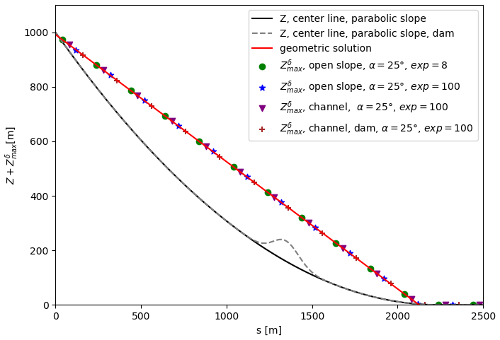
In addition, the model motivation allows prediction of the geometrically and theoretically expected solution in terms of runout and zδ. By comparing the geometrically correct solution zδ with the simulation results of for each scenario we obtain a match with the root mean squared error of for each simulation result compared with the geometric solution (see Fig. 6). This in turn validates the discretized model equations and their correct implementation. That is, the cell-by-cell approach to the routing results in expected behavior with all the stopping points matching the geometric solution even on flat and uphill terrain with very high accuracy. Furthermore, values solved on the 10 m grid for each scenario fit the continuous geometric solution. This validation, however, is only relevant for the intensity and runout length along the centerline. It was not the aim to fully validate the implementation of the spreading algorithm; however, the scenarios show satisfying results wherein single flow and divergent flow behavior, i.e., ranges from block to fluvial GMF behavior, can be reproduced by changing the Flow-Py parameterization (Fig. 3).
This section is dedicated to highlighting the performance of the Flow-Py simulation tool in real terrain and on a regional scale by applying it to the snow avalanche GMF.
4.1 Study area description and experimental setup
The study area is located in the mountains surrounding the Austrian villages Vals and Gries am Brenner in Tyrol close to the Italian border (Plörer and Stöhr, 2021). The area of the study area is 104.5 km2. The input DEM is freely available from Land Tirol (data.tirol.gv.at) issued under a Creative Commons Attribution 4.0 International (CC BY 4.0) license.
The computation time is dependent on the number of starting cells and the extent of the paths (how divergent or concentrated). We developed an overly simple starting zone model to test the performance of Flow-Py on a regional scale. There are many models for identifying potential avalanche starting zones that use a range of slope inclinations such as 28 to 60∘ (Veitinger et al., 2016; Pistocchi and Notarnicola, 2013; Maggioni and Gruber, 2003). More information, such as terrain curvature, forest cover, and average maximum snow depth, is used to further restrict the number and size of potential starting zones. The starting zone model employed is based solely on the slope inclinations derived from the 10 m DEM with the goal to provide a sufficient number of starting cells with potentially long runout lengths for performance testing. To achieve this we used two criteria for identifying starting cells: first, starting cells must be located above 1800 m; second, the starting cell must have a slope inclination between 31 and 34∘. The range of slope inclinations used is much smaller than used in more sophisticated models. This method was used to reduce the number of starting cells without introducing more information, such as forest area or average snow depth, but rather relying solely on the 10 m DEM.
The parameterizations for this simulation were and exp=8 as well as and m, which have successfully been used to model large to very large avalanches (D’Amboise et al., 2021b). For snow avalanches an exp of 8 on a 10 m resolution DEM has produced good results in past studies (Huber et al., 2016).
4.2 Results
The study area contains 1 045 311 raster cells (104 531 100 m2), and starting cells comprise 5.4 % of the total study area (56 969 raster cells or 5 696 900 m2), which can be seen in Fig. 7. The simulation took 3 h and 45 min with multi-processing on 16 cores.
Flow-Py identified 642 630 cells or 61.5 % of the total study area as part of the avalanche starting, transit, and runout zones (see Fig. 8). Many of these cells belong to multiple paths and are therefore base cells for many calculations, which is reflected in the CC (cell counts) output raster. The CC output is not shown; however, all the example input data and simulation results can be found in D'Amboise et al. (2021a).
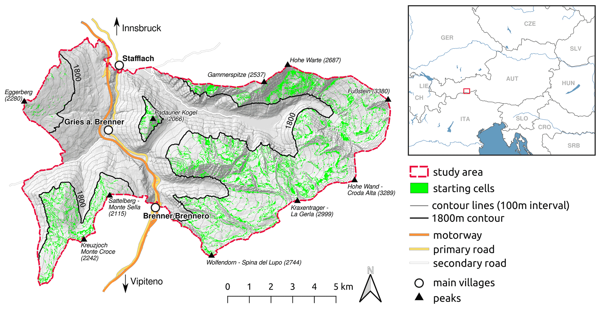
Figure 7Study area for Flow-Py performance testing on a regional scale. Snow avalanche starting cells (green) are defined by locations above 1800 m on slope inclinations between 31 and 34∘. The maps utilize datasets from the following sources. (a) ©OpenStreetMap contributors 2021. Distributed under the Open Data Commons Open Database License (ODbL) v1.0. (b) Natural Earth. Free vector and raster map data at https://www.naturalearthdata.com/ (last access: 1 October 2021). (c) Land Tirol – https://www.tirol.gv.at/statistik-budget/tiris/ (last access: 1 March 2021), issued under a Creative Commons Attribution 4.0 International (CC BY 4.0) license.
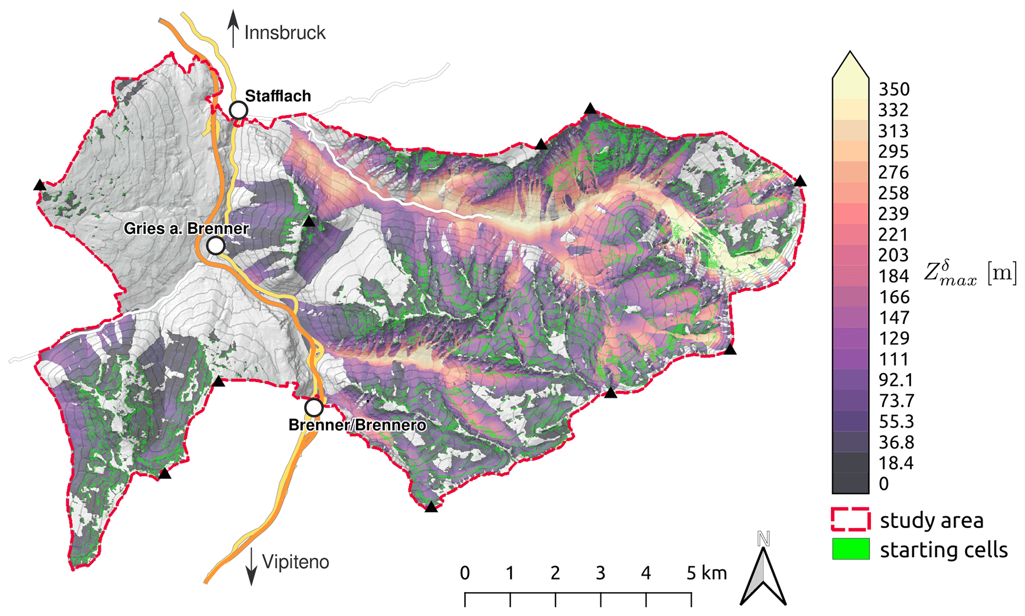
Figure 8Flow-Py simulation results of snow avalanche runout and intensity () in complex terrain on a regional scale. The simulation took 3 h and 45 min. The map utilizes data from ©OpenStreetMap contributors 2021. Distributed under the Open Data Commons Open Database License (ODbL) v1.0 and Land Tirol (https://www.tirol.gv.at/statistik-budget/tiris/, last access: 1 March 2021) issued under a Creative Commons Attribution 4.0 International (CC BY 4.0) license.
4.3 Discussion
The GMF path (extent of the avalanche starting, transit, and runout zones) is determined by the length of runout and the amount of spreading. Because of the overly simple starting zone model used, these results should not be used to examine the avalanche situation in the study area, but rather for demonstrating the computational performance of Flow-Py. In this example, the dominant term that determines the runout length is the runout angle α, but it can also be affected by . The dominant terms that determines the spreading of the process are the divergence (exp) and flux cutoff (Rstop). Combined, they can also limit the runout length when Rstop is high or divergence (low exp values) is excessively high. However, the feedback that propagates between the routines should not be ignored. A large runout angle (short runout length) will restrict the spreading capabilities even when using a low exp for a highly divergent process.
The parameterization used in this example has been used in past work for simulations of extreme avalanche events (D’Amboise et al., 2021b); however, there is a need for much more extensive parameter studies, in particular how exp and Rstop interact to limit the spreading of the GMF and the use of to limit the reach of the GMF.
The run time of simulations is highly dependent on the scenario and parameter setting. For Flow-Py we showed that the simulation run time in the parabolic slope example varies by an order of magnitude by changing the divergence parameter, exp (compare Fig. 3a and b). The run time is affected to a lesser extent by the number of starting cells and the length of the runout.
The comparison of computational efficiency of GMF simulation tools is not a trivial task because there is a lack of standardized examples and parameterizations used for benchmarking. More specifically, these tests are restricted by limited model access, and simulation tools belonging to the data-based class of models require a spatial iteration wherein process-based models solve the equations of motion and therefore the spatial–temporal flow evolution. Since the solver and parameterization differ drastically a direct comparison is not possible for different modeling approaches. Values in the literature vary significantly for the different types of simulation tools (Fischer et al., 2020; Rauter et al., 2018), so their potential for comparison is limited due to the already mentioned variation in scenarios and parameter setting but also the different computer hardware used to test the simulation tools, ranging from personal computers to cloud computing approaches. However, a comparison of simulations run on the same hardware that result in a similar spatial extent can be used to gain insight on computational efficiency and simulation run time.
To provide an estimate of computational efficiency we compared Flow-Py simulations with the open-source process-based physical simulation tool AvaFrame Com1DFA (Wirbel et al., 2021). Flow-Py and Com1DFA simulations were run on a personal computer with an eight-core processor (AMD Ryzen 7 2700X eight-core Processor 3.70 GHz) and 32 GB RAM. For the parabolic slope example (Fig. 3) it turned out that Flow-Py requires 1–2 orders of magnitude less computational time than Com1DFA using operational standard parameters (e.g., 5 m computational resolution compared to 10 m in the Flow-Py example) for avalanches of catastrophic size and an estimated release thickness of 1 m as required input.
The third computational experiment highlights the adaptability of the Flow-Py simulation tool with an example for a custom extension that was designed to answer a specific question, but additional information and calculations can be easily added into the Flow-Classes (Neuhauser et al., 2021).
5.1 Experimental setup and methods
This specific model customization experiment addresses this research question: what areas on the terrain are associated with endangering a location containing infrastructure by a GMF? For this example the parabolic slope from Sect. 3.1 and release raster from Sect. 3 were used as input data with the parameterization , exp=8, , and m as well as an additional input raster that contains the location of infrastructure. With the experimental setup defined the initial question can be refined: what raster cells on the synthetic parabolic slope are associated with routing flux of an GMF through a specific set of raster cells that have been identified as locations with infrastructure?
A custom extension called the back-tracking extension was implemented to change the runout model to a model that highlights terrain associated with endangering infrastructure. The back-tracking results will be a spatially explicit subset of the GMF path. Three steps are required to adjust the Flow-Py simulation tool.
-
Load the infrastructure raster as an additional input raster.
-
Adjust the calculation and store new information in the Flow-Class.
-
Save the back-tracking information as a raster and discard the default outputs.
Steps 1 and 3 are simple tasks when using the existing input and outputs of Flow-Py as an example. For the version of Flow-Py used in this contribution an automatic switch was added such that, when an additional input raster is included, Flow-Py will initiate the back-tracking extension and suppress the normal Flow-Py outputs (see the Flow-Py repository in Neuhauser et al., 2021, for more information on implementing these steps).
Step 2 is the more challenging adjustment that highlights the adaptable nature of the Flow-Class organization. Since the goal of back-tracking is to find the avalanche starting, transit, and runout zones that are associated with endangering infrastructure, a new back-tracking variable must be added to the Flow-Class storing information about a cell's parents. If the back-tracking variable of a cell is 0, then this cell is not associated with endangering infrastructure; if it is 1, then the cell is associated with endangering infrastructure. After a path is calculated and before updating the result raster, the back-tracking routine can start. Starting with the cells identified as a location with infrastructure a family tree can be constructed by looking at which cells acted as parent cells to these infrastructure cells. For each parent cell the back-tracking variable is changed from 0 to 1. After looping over all cells identified as parent cells that are related to cells containing infrastructure, the result raster can be updated with the back-tracking results and the next GMF starting cell can be calculated.
To optimize the back-tracking extension with regards to model run time, the starting cells have been ordered by elevation. If a starting cell is located in the path of a previously calculated starting cell at a higher elevation, then the lower-elevation starting cell is removed from the queue of starting cells that must be calculated. This will greatly reduce the run time of the model as fewer starting cells and process paths need to be computed; however, no information about the back-tracking is lost because the process path of the lower starting cell will be a subset of the upper starting cell's path, but other output rasters such as cell counts (CC) and the will no longer be valid since some starting cells are ignored for optimization.
To test the back-tracking extension two types of infrastructure were considered: a linear infrastructure such as a road, railroad, or walking path that crosses the terrain and a single pixel which could represent a building or utility pole.
5.2 Results
Figure 9a shows linear infrastructure (vertical red line) crossing the parabolic terrain, with the areas identified by the back-tracking extension. Most of the path located uphill of the infrastructure has been identified by the back-tracking extension except for a few cells that lay on its edges. This is because these cells were not parent cells due to the routing-flux-induced stopping criterion.
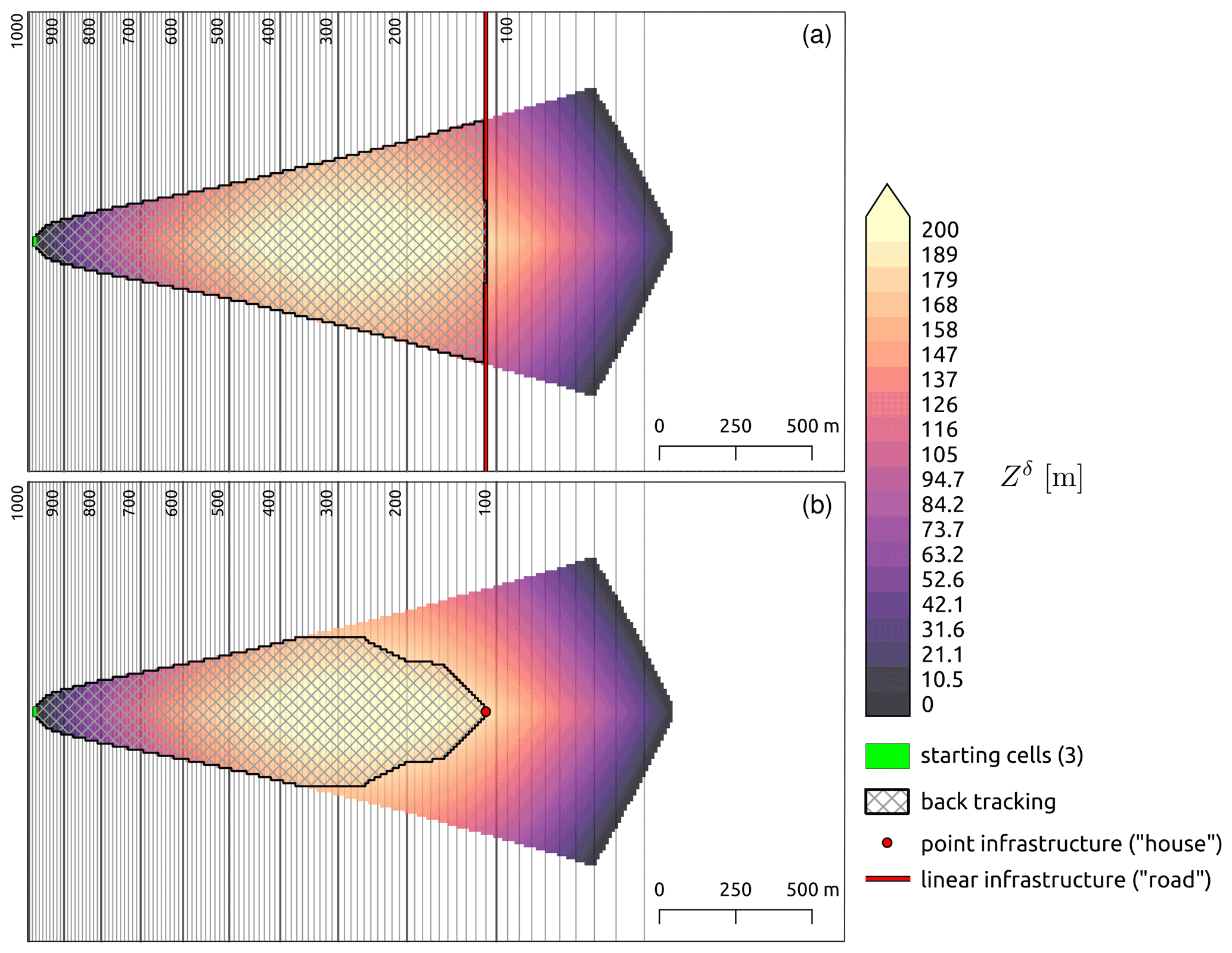
Figure 9GMF runout modeled with Flow-Py and results of the back-tracking extension with , exp=8, , and m. The textured areas highlight starting, transit, or runout zones associated with endangering linear infrastructure (a) or a building (b). The topography is a simple parabolic slope connected to a flat plane.
The bottom panel of Fig. 9 shows how the back-tracking extension behaves for a single infrastructure cell (red), e.g., a building, in the center of the GMF path. A wedge-shaped subset of the process path starting at the infrastructure cell and extending upslope is identified by the back-tracking extension, and it is clearly shown that not all uphill cells of the infrastructure cell route flux through the infrastructure cell. In both linear and building infrastructure cases, all cells that lay below the infrastructure cells are not identified by the back-tracking extension.
5.3 Discussion
The back-tracking extension is a complex adaptation because inputs, outputs, and some calculations are changed. However, because of the modular and adaptive Flow-Py development environment and the advantages of programming in Python's object-oriented class method, this complex task could be adopted with little effort.
Different routing or stopping approaches could also be easily added to the Flow-Class, which may be necessary to represent different types of GMFs more precisely. For instance, the additional energy dissipation due to terrain roughness or forest can be included by accepting different runout angles in the Flow-Class (D’Amboise et al., 2021b) as well as a Voellmy-type friction term (Voellmy, 1955), which is dependent on the GMF intensity (). Moreover, material flowing versus material sliding or falling downslope behaves differently, which could be described more precisely in the Flow-Py simulation tool by including different routing and stopping routines, such as the TauDEM routing for snow avalanches (Tarboton et al., 2015) or a steepest decent single flow method (Huggel et al., 2003). However, many of potential Flow-Py extensions will include one or more of the three steps outlined with the back-tracking examples (i.e., load additional input, adjust the calculation, or save additional output).
We used the back-tracking extension to exemplify and highlight the adaptability of the Flow-Py simulation tool. By making small adaptions Flow-Py was changed from a runout model to a model that identifies endangered infrastructure, which demonstrates how Flow-Py can be used to investigate questions related to specific GMFs.
Flow-Py is an open-source simulation tool for data-based gravitational mass flow (GMF) runout and intensity modeling, which is suitable for spatially explicit applications on a regional scale. GMF is a term that generalizes the flow of various materials in different ratios of solids, water (ice), and air down a slope. The GMF behavior, the runout length, and the amount of lateral spreading are all partially dependent on the composition of the material (Pudasaini and Mergili, 2019). Flow-Py handles diverse flow behaviors by providing an adjustable parameterization that acts to control the spreading and runout lengths of the simulated GMF path.
Flow-Py's basic model equations and well-organized solver split the GMF runout modeling into two routines: (1) routing of the GMF and (2) stopping of the GMF. The routing routine is further broken down into terrain-based and persistence-based routing, and the stopping routine is further broken down into two stopping criteria based on runout length and the amount of flux. With this, Flow-Py provides an educational GMF model development environment, which combines computational efficiency with low entry barriers for adaptations and extension, such as the presented back-tracking extension.
Besides the local topography two factors influence the spreading of the simulated GMF, namely the exp parameter and the routing flux threshold Rstop. However, the four main parameters (runout angle α, divergence control exp, flux cutoff Rstop, and the limit of the process intensity ) have to be defined based on one's experience or corresponding guidelines to obtain the desired range of motion behaviors corresponding to different materials and their compositions. However, further studies are needed for in-depth parameter investigations, including the development of parameter sets which can be used for specific GMF types such as rockfall, different types of snow avalanches, or landslides. Some of these parameter studies should include a sensitivity study on the DEM resolution used.
The implementation of the model equations to route the flux on the cell level has the advantage that the flow path does not need to be predetermined in contrast to some similar statistical runout methods (Lied and Bakkehøi, 1980). Therefore, Flow-Py combines the simplicity of a runout-angle-motivated model with the advantages associated with process-based modeling, providing a corresponding intensity measure and allowing for routing in flat or uphill terrain as we demonstrated in a computational experiment.
The results of a second experiment show that the run time of the model is suitable for regional modeling (several 100 km2) (see Sect. 4). The main factor that controls model run time is the parameterization, especially the amount of spreading, which is controlled by exp and Rstop; however, the number of starting cells and the number of available computer cores are also important factors influencing model run time.
One of the major benefits of Flow-Py compared to existing GMF simulation tools is its well-organized code that allows easy adaptations and extension development. A custom extension was developed for Flow-Py to take into account terrain complexity with regards to snow avalanches; automated avalanche terrain exposure scale (ATES) maps were created (Larsen et al., 2020). Future work is being carried out to develop a custom extension which will adapt the stopping criteria to other statistical models (Lied and Bakkehøi, 1980; Barbolini et al., 2011). We presented the back-tracking extension in Sect. 5 to demonstrate adaptability of the simulation tool, which required adjustments to the input data, calculations, and output raster. The additional calculations took advantage of Flow-Py's programming in Python's object-oriented class method, the Flow-Class. The output can be used to identify forests with a direct object protective function by combining the back-tracking results with a map of the current forest cover in a post-processing procedure. More simple extensions have already been developed and used, e.g., the forest extension, which has been applied to quantify the forest's protective effects in transit zones of rockfall and starting, transit, and runout zones of snow avalanches, as well as adapting the runout angle stopping criteria dependent on forest structure and the intensity () of the GMF (D’Amboise et al., 2021b).
We have shown that Flow-Py is an innovative GMF simulation tool that can be applied for basic simulations (e.g., for hazard zone mapping) but also for more sophisticated custom applications such as identifying areas that potentially endanger specific infrastructure. Furthermore, presenting Flow-Py in this contribution as well as the modeling concepts that motivated its model equations and their implementation in the Flow-Py code enables one to reproduce and understand the basic concepts of GMF modeling and to also use Flow-Py as an educational tool.
The Flow-Py code and user manual can be found in the repository in Neuhauser et al. (2021).
Input data and simulation results can be found in D'Amboise et al. (2021a).
MN developed the model code with help from JTF and CJLD. Original draft preparation was done by CJLD and JTF with significant input from MN (model description) and MT (introduction and conclusions). Figures were designed by AH, MN, and CJLD. Model conceptualization was performed by RF, AH, AK, FP, JTF, MN, and CJLD with overarching research goals formulated by KK and JTF. Data (DEMs) were obtained and/or created by JTF and CJLD. Funding was acquired by FP, MT, JTF, and MT. All authors supported the review and editing process of the paper.
The contact author has declared that neither they nor their co-authors have any competing interests.
Publisher's note: Copernicus Publications remains neutral with regard to jurisdictional claims in published maps and institutional affiliations.
This work was conducted in the context of the GreenRisk4ALPs project (ASP635), which has been financed by Interreg Alpine Space, one of the 15 transnational cooperation programs covering the whole of the European Union (EU) in the framework of European regional policy. Additional financial support came from AvaRange (https://www.avarange.org/, last access: 1 February 2022; international cooperation project “AvaRange – Particle Tracking in Snow Avalanches” supported by the German Research Foundation; DFG, DR 639/22-1), the Austrian Science Fund (FWF, I 4274-N29), and the open Avalanche Framework AvaFrame (https://www.avaframe.org/, last access: 1 March 2022). AvaFrame is a cooperation between the Austrian Research Centre for Forests (Bundesforschungszentrum für Wald; BFW) and the Austrian Avalanche and Torrent Service (Wildbach- und Lawinenverbauung; WLV) in conjunction with the Federal Ministry Republic of Austria: Agriculture, Regions and Tourism (BMLRT).
This paper was edited by Heiko Goelzer and reviewed by two anonymous referees.
Ancey, C., Meunier, M., and Richard, D.: Inverse problem in avalanche dynamics models, Water Resour. Res., 39, 1099, https://doi.org/10.1029/2002WR001749, 2003. a
Bakkehøi, S., Domaas, U., and Lied, K.: Calculation of snow avalanche runout distance, Ann. Glaciol., 4, 24–29, 1983. a, b
Barbolini, M., Gruber, U., Keylock, C. J., Naaim, M., and Savi, F.: Application of statistical and hydraulic-continuum dense-snow avalanche models to five real European sites, Cold Reg. Sci. Technol., 31, 133–149, 2000. a
Barbolini, M., Pagliardi, M., Ferro, F., and Corradeghini, P.: Avalanche hazard mapping over large undocumented areas, Nat. Hazards, 56, 451–464, 2011. a, b, c
Brenning, A.: Spatial prediction models for landslide hazards: review, comparison and evaluation, Nat. Hazards Earth Sys., 5, 853–862, 2005. a
Christen, M., Bartelt, P., and Gruber, U.: AVAL-1D: An avalanche dynamics program for the practice, in: International Congress Interpraevent 2002 in the Pacific Rim – Matsumoto/Japan, Congress publication, 2, 715–725, 2002. a
Christen, M., Kowalski, J., and Bartelt, P.: RAMMS: Numerical simulation of dense snow avalanches in three-dimensional terrain, Cold Reg. Sci. Technol., 63, 1–14, 2010. a, b
Corominas, J., van Westen, C., Frattini, P., Cascini, L., Malet, J.-P., Fotopoulou, S., Catani, F., Van Den Eeckhaut, M., Mavrouli, O., Agliardi, F., and Pitilakis, K.: Recommendations for the quantitative analysis of landslide risk, B. Eng. Geol. Environ., 73, 209–263, 2014. a, b
Crozier, M. J. and Glade, T.: Landslide hazard and risk: issues, concepts and approach, Landslide hazard and risk, chap. 1, 1–40, https://doi.org/10.1002/9780470012659.ch1, 2005. a
D'Amboise, C. J. L., Neuhauser, M., Teich, M., and Fischer, J.-T.: Maverick-bfw/Flow_py_inputs_results: First releases (Version v1), Zenodo [data set], https://doi.org/10.5281/zenodo.5154787, 2021a. a, b
D’Amboise, C. J. L., Teich, M., Hormes, A., Steger, S., and Berger, F.: “Modeling Protective Forests for Gravitational Natural Hazards and How It Relates to Risk-Based Decision Support Tools”, in: Protective forests as Ecosystem-based solution for Disaster Risk Reduction (ECO-DRR), edited by: edited by: Teich, M., Accastello, C., Perzl, F., and Kleemayr, K., London: IntechOpen, https://www.intechopen.com/online-first/78979 (last access: 1 March 2022), 2021b. a, b, c, d
Dorren, L.: A review of rockfall mechanics and modelling approaches, Prog. Phys. Geog., 27, 69, https://doi.org/10.1191/0309133303pp359ra, 2003. a
Dorren, L.: Rockyfor3D (v4.1) revealed – Transparent description of the complete 3D rockfall model, ecorisQ paper, https://www.ecorisq.org/ (last access: 1 June 2021), 2012. a
Dorren, L. K., Domaas, U., Kronholm, K., and Labiouse, V.: Methods for predicting rockfall trajectories and runout zones, edited by: Lambert, S., Tech. Rep., John Wiley & Sons, ISTE Ltd, 143–173, ISBN 9781848212565, 2011. a
Eckert, N., Naaim, M., and Parent, E.: Long-term avalanche hazard assessment with a Bayesian depth-averaged propagation model, J. Glaciol., 56, 563–586, 2010. a
Fell, R., Corominas, J., Bonnard, C., Cascini, L., Leroi, E., Savage, W. Z., and the JTC-1 Joint Technical Committee on Landslides and Engineered Slopes: Guidelines for landslide susceptibility, hazard and risk zoning for land-use planning, Eng. Geol., 102, 99–111, 2008. a
Fischer, J. T., Kofler, A., Fellin, W., Granig, M., and Kleemayr, K.: Multivariate parameter optimization for computational snow avalanche simulation, J. Glaciol., 61, 875–888, https://doi.org/10.3189/2015JoG14J168, 2015. a
Fischer, J.-T., Kofler, A., Huber, A., Fellin, W., Mergili, M., and Oberguggenberger, M.: Bayesian Inference in Snow Avalanche Simulation with r. avaflow, Geosciences, 10, 191, https://doi.org/10.3390/geosciences10050191, 2020. a
Fressard, M., Thiery, Y., and Maquaire, O.: Which data for quantitative landslide susceptibility mapping at operational scale? Case study of the Pays d'Auge plateau hillslopes (Normandy, France), Nat. Hazards Earth Syst. Sci., 14, 569–588, https://doi.org/10.5194/nhess-14-569-2014, 2014. a
Fuchs, S., Thöni, M., McAlpin, M. C., Gruber, U., and Bründl, M.: Avalanche hazard mitigation strategies assessed by cost effectiveness analyses and cost benefit analyses – evidence from Davos, Switzerland, Nat. Hazards, 41, 113–129, 2007. a
Gamma, P.: dfwalk - Ein Murgang-Simulationsprogramm zur Gefahrenzonierung, PhD thesis, G66, Universität Bern, 1999. a, b
Guillard, C. and Zezere, J.: Landslide susceptibility assessment and validation in the framework of municipal planning in Portugal: the case of Loures Municipality, Environ. Manage., 50, 721–735, 2012. a
Guzzetti, F., Crosta, G., Detti, R., and Agliardi, F.: STONE: a computer program for the three-dimensional simulation of rock-falls, Comput. Geosci., 28, 1079–1093, 2002. a, b
Heim, A.: Bergstürze und Menschenleben, in: Beiblatt zur Vierteljahrsschrift der Naturforschenden Gesellschaft in Zürich Publisher, Zürich, Fretz & Wasmuth, 1932. a, b, c, d, e
Holmgren, P.: Multiple flow direction algorithms for runoff modelling in grid based elevation models: an empirical evaluation, Hydrol. Proc., 8, 327–334, 1994. a, b, c, d
Horton, P., Jaboyedoff, M., Rudaz, B., and Zimmermann, M.: Flow-R, a model for susceptibility mapping of debris flows and other gravitational hazards at a regional scale, Nat. Hazards Earth Syst. Sci., 13, 869–885, https://doi.org/10.5194/nhess-13-869-2013, 2013. a, b, c, d, e, f, g, h, i
Huber, A., Fischer, J. T., Kofler, A., and Kleemayr, K.: Using spatially distributed statistical models for avalanche runout estimation, in: International Snow Science Workshop, Breckenridge, Colorado, USA, 2016. a, b
Huggel, C., Kääb, A., Haeberli, W., and Krummenacher, B.: Regional-scale GIS-models for assessment of hazards from glacier lake outbursts: evaluation and application in the Swiss Alps, Nat. Hazards Earth Syst. Sci., 3, 647–662, https://doi.org/10.5194/nhess-3-647-2003, 2003. a, b
Huggel, C., Caplan-Auerbach, J., Waythomas, C., and Wessels, R.: Monitoring and modeling ice-rock avalanches from ice-capped vocanoes: A case study of frequent large avalanches of Iliamna Volcano, Alaksa, J. Volcanol. Geoth. Res., 168, 114–136, 2007. a
Köhler, A., McElwaine, J., and Sovilla, B.: GEODAR data and the flow regimes of snow avalanches, J. Geophys. Res.-Earth, 123, 1272–1294, 2018. a
Körner, H.: The energy-line method in the mechanics of avalanches, J. Glaciol., 26, 501–505, 1980. a, b
Larsen, H., Sykes, J., Schauer, A., Hendrikx, J., Langford, R., Statham, G., Campbell, C., Neuhauser, M., and Fischer, J. T.: Development of automated avalanche terrain exposure scale maps: current and future, in: Virtual Snow Science Workshop, Fernie, Canada, 2020. a
Lied, K. and Bakkehøi, S.: Empirical calculations of snow-avalanche run-out distance based on topographic parameters, J. Glaciol., 26, 165–177, 1980. a, b, c, d
Maggioni, M. and Gruber, U.: The influence of topographic parameters on avalanche release dimension and frequency, Cold Reg. Sci. Technol., 37, 407–419, https://doi.org/10.1016/S0165-232X(03)00080-6, 2003. a
McClung, D. and Lied, K.: Statistical and geometrical definition of snow avalanche runout, Cold Reg. Sci. Technol., 13, 107–119, 1987. a
Mergili, M., Krenn, J., and Chu, H.-J.: r.randomwalk v1, a multi-functional conceptual tool for mass movement routing, Geosci. Model Dev., 8, 4027–4043, https://doi.org/10.5194/gmd-8-4027-2015, 2015. a
Mergili, M., Fischer, J.-T., Krenn, J., and Pudasaini, S. P.: r.avaflow v1, an advanced open-source computational framework for the propagation and interaction of two-phase mass flows, Geosci. Model Dev., 10, 553–569, https://doi.org/10.5194/gmd-10-553-2017, 2017. a
Moos, C., Fehlmann, M., Trappmann, D., Stoffel, M., and Dorren, L.: Integrating the mitigating effect of forests into quantitative rockfall risk analysis–Two case studies in Switzerland, Int. J. Disast. Risk Re., 32, 55–74, 2018. a
Neuhauser, M., D'Amboise, C., Teich, M., Kofler, A., Huber, A., Fromm, R., and Fischer, J. T.: Flow-Py: routing and stopping of gravitational mass flows, Zenodo [code], https://doi.org/10.5281/zenodo.5027274, 2021. a, b, c, d, e
Noetzli, J., Huggel, C., Hoelzle, M., and Haeberli, W.: GIS-based modelling of rock-ice avalanches from Alpine permafrost areas, Computat. Geosci., 10, 161–178, 2006. a
Okuda, S.: Rapid mass movements, Field Experiments and Measurement Programs in Geomorphology, edited by: Slaymaker, O., CRC Press, 61–105, ISBN 9789061919964, 1991. a
Pistocchi, A. and Notarnicola, C.: Data-driven mapping of avalanche release areas: a case study in South Tyrol, Italy, Nat. Hazards, 65, 1313–1330, 2013. a
Plörer, M. and Stöhr, D.: Gries am Brenner/Vals Pilot Action Region: The Tyrolean Ski Tour Steering Concept – A Contribution to the Protection of Wildlife and Object Protective Forests in Best Practice Examples of Implementing Ecosystem-Based Natural Hazard Risk Management in the GreenRisk4ALPs Pilot Action Regions, edited by: Beguš, J., Berger, F., and Kleemayr, K., London, IntechOpen, https://doi.org/10.5772/intechopen.99011, 2021. a
Pudasaini, S. P. and Mergili, M.: A multi-phase mass flow model, J. Geophys. Res.-Earth, 124, 2920–2942, 2019. a
Rauter, M., Kofler, A., Huber, A., and Fellin, W.: faSavageHutterFOAM 1.0: depth-integrated simulation of dense snow avalanches on natural terrain with OpenFOAM, Geosci. Model Dev., 11, 2923–2939, https://doi.org/10.5194/gmd-11-2923-2018, 2018. a
Sampl, P. and Granig, M.: Avalanche simulation with SAMOS-AT, in: Proceedings of the International Snow Science Workshop, Montana State University Library, Davos, 27, 519–523, 2009. a
Sampl, P. and Zwinger, T.: Avalanche simulation with SAMOS, Ann. Glaciol., 38, 393–398, 2004. a
Sauermoser, S.: Avalanche hazard mapping – 30 years experience in Austria, in: Proceedings of the 2006 International Snow Science Workshop in Telluride, Colorado, 1–6, Citeseer, 2006. a
Scheidl, C. and Rickenmann, D.: TopFlowDF - a simple GIS based model to simulate debris-flow runout on the fan., in: Proceedings of the 5th international Conference on Debris-Flow Hazards: Mitigation, Mechanics, Prediction and Assessment, edited by: Genevois, R., Hamiltion, D., and Prestininzi, A., 253–262, https://doi.org/10.4408/IJEGE.2011-03.B-030, 2011. a
Tarboton, D. G., Dash, P., and Sazib, N.: TauDEM 5.3: Guide to Using the TauDEM Command Line Functions, 2015. a
Teich, M. and Bebi, P.: Evaluating the benefit of avalanche protection forest with GIS-based risk analyses – A case study in Switzerland, Forest Ecol. Manag., 257, 1910–1919, 2009. a
Van Rossum, G. and Drake, F. L.: Python 3 Reference Manual, CreateSpace, Scotts Valley, CA, ISBN 9781441412690, 2009. a
Van Westen, C., Van Asch, T. W., and Soeters, R.: Landslide hazard and risk zonation—why is it still so difficult?, B. Eng. Geol. Environ., 65, 167–184, 2006. a
Van Westen, C. J., Castellanos, E., and Kuriakose, S. L.: Spatial data for landslide susceptibility, hazard, and vulnerability assessment: An overview, Eng. Geol., 102, 112–131, 2008. a
Varnes, D. J.: Slope movement types and processes, Transportation Research Board Special Report, 176, 11–33, 1978. a, b
Veitinger, J., Purves, R. S., and Sovilla, B.: Potential slab avalanche release area identification from estimated winter terrain: a multi-scale, fuzzy logic approach, Nat. Hazards Earth Syst. Sci., 16, 2211–2225, https://doi.org/10.5194/nhess-16-2211-2016, 2016. a
Voellmy, A.: Über die Zerstörungskraft von Lawinen, Schweizerische Bauzeitung, Sonderdruck aus dem 73. Jahrgang, 1–25, 1955. a
Wichmann, V.: The Gravitational Process Path (GPP) model (v1.0) – a GIS-based simulation framework for gravitational processes, Geosci. Model Dev., 10, 3309–3327, https://doi.org/10.5194/gmd-10-3309-2017, 2017. a, b
Wirbel, A., Oesterle, F., Tonnel, M., and Fischer, J.-T.: avaframe/AvaFrame: Version 0.5, Zenodo [code], https://doi.org/10.5281/zenodo.5094509, 2021. a, b, c
- Abstract
- Introduction
- Model description
- Model testing and validation on generic slopes
- Performance testing on a regional scale
- Model customization and adaptability
- Conclusions and outlook
- Code and data availability
- Author contributions
- Competing interests
- Disclaimer
- Acknowledgements
- Review statement
- References