Impacts of a revised surface roughness parameterization in the Community Land Model 5.1

The roughness of the land surface (z₀) is a key property, exerting significant influence on the amount of near-surface turbulent activity and consequently the turbulent exchange of energy, water, momentum, and chemical species between the land and the atmosphere. Variations in z₀ are substantial across different types of land cover, ranging from typically less than 1 mm over fresh snow or sand deserts up to more than 1 m over urban areas or forests. In this study, we revise the parameterizations and parameter choices related to z₀ in the Community Land Model 5.1 (CLM), the land component of the Community Earth System Model (CESM). We propose a number modifications for z₀ in CLM, guided by observational data. Most importantly, we find that the observations support an increase in z₀ for all types of forests and a decrease in the momentum z₀ for bare soil, snow, glaciers, and crops. We then assess the effect of those modifications in land-only and land–atmosphere coupled simulations. With the revised parameterizations, diurnal variations of the land surface temperature (LST) are dampened in forested regions and are amplified over warm deserts. These changes mitigate model biases compared to MODerate resolution Imaging Spectroradiometer (MODIS) remote sensing observations. The changes in LST are generally stronger during the day than at night. For example, the LST increases by 5.1 K at 13:30 local solar time but only by 0.6 K at 01:30 during boreal summer across the entire Sahara. The induced changes in the diurnal variability of near-surface air temperatures are generally of the opposite sign and of smaller magnitude. Near-surface winds accelerate in areas where the momentum z₀ was lowered, such as the Sahara, the Middle East, and Antarctica, and decelerate in regions with forests. Overall, this study finds that the current representation of z₀ in CLM is not in agreement with observational constraints for several types of land cover. The proposed model modifications are shown to considerably alter the simulated climate in terms of temperatures and wind speed at the land surface.

1 Introduction

The land surface interacts in numerous ways with the atmosphere. Among the most relevant interactions is the turbulent exchange of sensible heat, water vapor, momentum, and chemical species at the land–atmosphere interface. Turbulence above the land surface occurs due to the retardation of moving air by friction and due to the buoyancy created by surface heating from solar irradiance (Bonan, 2019). The intensity of the turbulence generated by friction is determined by the amount and shape of obstacles on land in concert with atmospheric conditions. In land models, the turbulent exchange with the atmosphere is commonly represented through the Monin–Obukhov similarity theory (MOST). A key parameter in MOST is the aerodynamic or momentum surface roughness, z_0m. A rough surface, such as an urban environment or a forest, is characterized by a higher z_0m and therefore induces more turbulence for a given wind speed than a smooth surface, such as a snow field or a lake. Similar surface roughness parameters exist for the exchange of scalars (e.g., temperature and water vapor). Observed values of z_0m over land span more than 4 orders of magnitude with values ranging from a few tenths of a millimeter over fresh snow (Brock et al., 2006) or bare soil (Prigent et al., 2005) to several meters over forests (Hu et al., 2020) or urban areas (Kanda et al., 2013).

The momentum surface roughness is defined as the height above the displacement height (d) where the average wind speed extrapolates to zero under neutral conditions. The displacement height accounts for the fact that large roughness elements, such as trees or buildings, may shift the logarithmic wind speed profile (which occurs under neutral conditions) upwards, such that mean wind speed extrapolates to zero at the height z_0m+d rather than z_0m. Similarly, the sensible heat (z_0h) and the latent heat (z_0q) roughness lengths are defined as the heights above d where the air temperature and the specific humidity reach their respective surface value under neutral conditions. In the surface sublayer, a thin layer of air directly adjacent to the surface of typically 10⁻³ to 10⁻¹ m thickness, water vapor and heat are transported solely through molecular diffusion, while momentum exchange is also facilitated by pressure fluctuations that are induced by the presence of roughness elements (Zeng and Dickinson, 1998). As a result, the turbulent exchange of sensible and latent heat between the land and the atmosphere is generally less efficient than the exchange of momentum. Accordingly, z_0h and z_0q are often much smaller than z_0m (Yang et al., 2002, 2008; Hu et al., 2020).

In the field, z₀ is commonly estimated through four main methods. The first approach is to measure the vertical wind speed profile and link these measurements to z_0m using the equation below (e.g., Greeley et al., 1997; Brock et al., 2006; Marticorena et al., 2006; Nakai et al., 2008; Hugenholtz et al., 2013; Kanda et al., 2013; Nield et al., 2013; Fitzpatrick et al., 2019). The wind speed profile is logarithmic under neutral conditions over a plain surface:

$$\begin{array}{}\text{(1)}& u\left(z\right)={\displaystyle \frac{u_{*}}{\mathit{\kappa }}}\ln \left({\displaystyle \frac{z-d}{z_{\mathrm{0}\mathrm{m}}}}\right),\end{array}$$

where u(z) is the mean wind speed profile, z is the height above the surface, u_* is the friction velocity, and κ is the von Karman constant (=0.4). This approach can also be used to estimate z_0h and z_0q through measurements of the temperature and specific humidity profiles. A second method is to use eddy covariance measurements of the momentum, the sensible heat, and latent heat fluxes, which can then be used to deduce the z_0m, z_0h, and z_0q that conform best with the measured fluxes according to MOST (e.g., Maurer et al., 2013; Li et al., 2015; Hu et al., 2020). A third method involves using measurements of the microtopography to link z_0m to small-scale variations of the height of the surface (e.g., Brock et al., 2006; Weligepolage et al., 2012; Hugenholtz et al., 2013; Fitzpatrick et al., 2019; van Tiggelen et al., 2021). The final approach uses remote sensing observations of either backscattering at the land surface or the surface reflectance to serve as a proxy for microtopography to estimate z_0m (e.g., Greeley et al., 1997; Marticorena et al., 2004; Prigent et al., 2005, 2012; Stilla et al., 2020). This latter approach requires some in situ measurements of z_0m to establish a relationship between the remotely sensed proxy and z_0m.

The surface roughness plays a central role for atmospheric dynamics (Sud et al., 1988; Vautard et al., 2010; Wever, 2012), energy fluxes at the land surface, and thereby temperatures at the land surface (Zeng and Dickinson, 1998; Zeng and Wang, 2007). Several studies have linked deficiencies of various models to a misrepresentation of z₀ (Chen et al., 2010; Subin et al., 2012; Zeng et al., 2012; Wang et al., 2014; Trigo et al., 2015; Xu et al., 2016; Wang et al., 2019). The aerodynamic z₀ also affects the simulated mineral dust emissions (Menut et al., 2013), which absorb and reflect solar radiation and thereby alter temperatures at the land surface (Claquin et al., 1998; Miller and Tegen, 1998; Klose et al., 2021). Further, alterations in z₀ due to de-, re-, and afforestation represent an important contribution to the biogeophysical effect of such land cover changes (Davin and de Noblet-Ducoudré, 2010; Lee et al., 2011; Burakowski et al., 2018; Belušić et al., 2019; Laguë et al., 2019; Winckler et al., 2019). Adequate parameterizations of z₀ are therefore not only crucial to realistically simulate climate and weather but also to understand the biogeophysical effects of land cover changes.

In this study, we revise the representation of z₀ in the Community Land Model version 5.1 (CLM; Lawrence et al., 2019), which is the land surface model of the Community Earth System Model (CESM; Danabasoglu et al., 2020). Our endeavors are motivated by an underestimation of diurnal variations in land surface temperature over arid and semi-arid regions in CLM/CESM (Zeng et al., 2012; Wang et al., 2014; Meier et al., 2019) as well as a seasonal cycle of z₀ for broadleaf deciduous forests that appears to be in opposition to observational data, as will be shown in the next section. In Sect. 2, we compare the representation of z₀ for each land cover type in CLM to observational data and parameterizations that have been proposed in the literature. Based on this comparison, we introduce five modifications to CLM: (1) a new parameterization of the vegetation z₀ based on Raupach (1992) with optimized parameters to match the data collected in Hu et al. (2020) for different types of vegetation; (2) new globally constant z_0m values for bare soil, snow, and glaciers based on field measurements; (3) inclusion of the parameterization of Yang et al. (2008) for z_0h and z_0q over bare soil, snow, and glaciers; (4) use of a spatially explicit z_0m input field for bare soil based on the data of Prigent et al. (2005); and (5) inclusion of the Brock et al. (2006) parameterization of z_0m for snow that is based on accumulated snowmelt. The latter two modifications replace the globally constant z_0m values for bare soil and snow and may therefore be activated individually by the model user. To assess the impact of these modifications, we then conduct land-only and land–atmosphere coupled simulations, as described in Sect. 3, and evaluate them as described in Sect. 4. Section 5 describes how our modifications of z₀ affect temperatures at the land surface and wind speed. We also confront the default and modified model configuration with MODerate resolution Imaging Spectroradiometer (MODIS) remote sensing observations of diurnal variations in the land surface temperature (LST) and the sensitivity of LST to a conversion of vegetation to bare land, based on the approach of Duveiller et al. (2018).

2 Revisions of surface roughness in CLM 5.1

2.1 General description of CESM and CLM

The Community Earth System Model is a state-of-the-art Earth system model, which is widely applied in the field of climate science and has contributed to multiple multi-model intercomparison projects. Version 2 was released in June 2018 (Danabasoglu et al., 2020), followed by several incremental releases to version 2.1.2, which is used in this study. The development of CESM is coordinated and led by the National Center for Atmospheric Research (NCAR). However, a number of additional universities and research institutes contribute to the development of CESM. It is publicly available and well documented to facilitate this community effort (https://www.cesm.ucar.edu/models/cesm2/, last access: 21 February 2022). CESM comprises prognostic components for the atmosphere, ocean, land, sea ice, land ice, rivers, and waves. Besides these prognostic components, an observed data version exists for most components. In these versions, the coupling fields of the respective components are prescribed from recent observational data instead of running this component prognostically. CESM therefore allows us to flexibly disable or enable coupling of model components depending on the application.

The Community Land Model is the land component of CESM. It comprehensively represents the surface energy fluxes, the surface hydrology, and optionally the biogeochemical cycles for carbon and nitrogen (Lawrence et al., 2018, 2019). Up to five different land units may exist in each grid cell: (naturally) vegetated, lakes, urban, glaciers, and crops. A land unit tile can be further divided into different columns (e.g., rainfed and irrigated for crops) and patches (e.g., different types of natural vegetation). Bare soil, which can be found frequently in arid regions, is treated as a patch of natural vegetation. These patches of natural vegetation are called plant functional types (PFTs). Vegetation is simulated by a big-leaf approach (Sellers et al., 1986), distinguishing between sunlit and shaded leaves. The vegetation phenology can either be prescribed from remote-sensing-based data (satellite phenology), which are used in this study, or computed prognostically from the vegetation carbon pools, if the biogeochemical cycle is activated.

CLM5 distinguishes between vegetation, bare soil, snow, glacier ice, lakes, and urban areas in its parameterization of z₀ (Lawrence et al., 2018). In the following sections, we describe the current representation of z₀ in CLM and our proposed modifications, which we justify by comparison to the literature. As mentioned, z_0m, z_0h, and z_0q correspond to the surface roughness for momentum, sensible heat, and latent heat, respectively. The land cover type is specified after a comma using “v”, “b”, “s”, “i”, and “g” for vegetated, bare soil, snow, ice (glaciers), and any type of ground (bare soil, snow, or ice), respectively (e.g., z_0h,b is the sensible heat surface roughness of bare soil). Note that z_0,v in CLM represents the aerodynamic roughness length for the turbulent exchange between the canopy air space and the free atmosphere. There is thus no distinction between z_0m,v, z_0h,v, and z_0q,v, as this exchange occurs above the surface sublayer. However, there are additional resistances between the leaves/ground and the canopy air space to account for the surface resistance of the sensible and latent heat fluxes. A list of the symbols and abbreviations used in this study is provided in Table A2.

2.2 Vegetation

The current representation of z_0,v and d was developed by Zeng and Wang (2007) and links these properties to the vegetation height (h_top), the exposed leaf area index (LAI; i.e., the one-sided leaf area above the snow, if there is any), and the exposed stem area index (SAI; i.e., the one-sided stem and dead leaf area above the snow) as follows (Eqs. 2.5.125–127 in Lawrence et al., 2018):

$$\begin{array}{}\text{(2)}& {\displaystyle }{z}_{\mathrm{0},\mathrm{v}}=\exp \left[V\ln \left(h_{\mathrm{top}}{R}_{z\mathrm{0}\mathrm{m}}\right)+(\mathrm{1}-V)\ln \left(z_{\mathrm{0}\mathrm{m},\mathrm{g}}\right)\right],\text{(3)}& {\displaystyle }d=h_{\mathrm{top}}{R}_{d}V,\text{(4)}& {\displaystyle }V={\displaystyle \frac{\mathrm{1}-\exp (-\mathit{\beta }min(\text{VAI},{\text{VAI}}_{\mathrm{cr}}\left)\right)}{\mathrm{1}-\exp (-\mathit{\beta }{\text{VAI}}_{\mathrm{cr}})}},\end{array}$$

where VAI is the vegetation area index defined as the sum of LAI and SAI, R_z0m and R_d are the ratios of z_0,v and d to the canopy height for values of VAI exceeding the critical value VAI_cr=2 m² m⁻², z_0m,g is the momentum surface roughness of the ground (see Sect. 2.3–2.5), V is a fractional weight, and β=1. R_z0m is set to 0.075 for broadleaf evergreen trees, to 0.055 for other trees, and to 0.12 for grass, crops, and shrubs, while R_d is 0.67 for all trees and 0.68 for grass, crops, and shrubs. With this implementation, $z_{\mathrm{0},\mathrm{v}}/h_{\mathrm{top}}$ increases almost linearly with VAI before plateauing at the constant value R_z0m beyond VAI_cr (red curves in the left column of Fig. 1).

Observations find a first-order linear relation between h_top and z_0,v as well as d (Tanner and Pelton, 1960). It is therefore common practice to normalize z_0,v by h_top when determining whether other vegetation properties influence z_0,v (Shaw and Pereira, 1982; Yang and Friedl, 2003; Zhou et al., 2006; Nakai et al., 2008; Maurer et al., 2015). Proposed parameterizations hence frequently link $z_{\mathrm{0},\mathrm{v}}/h_{\mathrm{top}}$ and $d/h_{\mathrm{top}}$ to other structural properties of the vegetation such as LAI, stand density, and/or crown width (Choudhury and Monteith, 1988; Raupach, 1992, 1994; Yang and Friedl, 2003; Nakai et al., 2008; Bingöl, 2019). For crops, z_0,v exhibits a distinct seasonal cycle in the extratropics, with low values during winter, when crops are absent (blue and turquoise lines in Fig. 1m; Hu et al., 2020; Young et al., 2021). On the other hand, z_0,v remains relatively high during the dormant phase if parts of the vegetation such as the stem and branches of trees persist throughout the year (Fig. 1b, d, and f; Dolman, 1986; Hu et al., 2020). In the case of broadleaf deciduous forests, there are even several studies that find a decrease in z_0,v for higher values of LAI, probably because the dense canopies during the growing season shelter the branches and trunks of trees from the atmospheric flow (Nakai et al., 2008; Maurer et al., 2013; Young et al., 2021).

Hu et al. (2020) provide z_0,v estimates for an extensive collection of FLUXNET sites, which offers an unprecedented opportunity to reconcile z_0,v values observed in the field and the z_0,v parameterizations in models. Here, we use an updated version of this data set for comparison to z_0,v in CLM, which is subsequently referred to as Hu20. This updated version includes more FLUXNET sites than the original publication. Hu20 estimates daily z_0,v values at a total of 113 FLUXNET sites by minimizing the following cost function J:

$$\begin{array}{}\text{(5)}& J=\sum (u_{*,\mathrm{obs}}-u_{*,\mathrm{est}}{)}^{\mathrm{2}},\end{array}$$

where $u_{*,\mathrm{obs}}$ is the measured friction velocity in the field and $u_{*,\mathrm{est}}$ the estimated friction velocity according to MOST:

$$\begin{array}{}\text{(6)}& u_{*,\mathrm{est}}=\mathit{\kappa }u{\left[\ln \left({\displaystyle \frac{z_{\mathrm{m}}-d}{z_{\mathrm{0},\mathrm{v}}}}\right)-{\mathrm{\Psi }}_{\mathrm{m}}\left({\displaystyle \frac{z_{\mathrm{m}}-d}{L}}\right)+{\mathrm{\Psi }}_{\mathrm{m}}\left({\displaystyle \frac{z_{\mathrm{0},\mathrm{v}}}{L}}\right)\right]}^{-\mathrm{1}},\end{array}$$

where u is the wind speed measured at the instrument height, z_m, d is the displacement height estimated as two-thirds of h_top, Ψ_m is the stability correction function for momentum transfer, and L is the Obukhov length scale. We divide the sites in Hu20 into the following six vegetation types: needleleaf forest, evergreen broadleaf forest, deciduous broadleaf forest, shrubland, grassland, and cropland. We make a number of additional suitability checks of the already quality-checked data, before using the data of Hu20 for comparison to CLM: (1) we exclude z_0,v values that deviate by more than 2 standard deviations from the mean z_0,v at the respective site; (2) we exclude z_0,v values when h_top=0, because we scale z_0,v by h_top in the next step; (3) we exclude sites that are not representative of the respective vegetation type according to a visual inspection on Google Maps (e.g., a sparse plantation); and (4) we remove sites with thin forest by excluding forest sites with a h_top below 5 m and/or a maximum fractional vegetation cover below 0.8. Finally, we assign the forest sites designated as mixed forest to the most abundant type of forest according the species composition as described in the respective publication. In addition to the mean annual cycle of z_0,v, we also consider the relationship between the VAI and $z_{\mathrm{0},\mathrm{v}}/h_{\mathrm{top}}$ in Hu20 to evaluate and revise the current parameterization in CLM. Hu20 provides LAI information but not SAI. Therefore, we extract from our CESM control simulation (Sect. 3) the monthly simulated SAI for the respective PFT and location, multiply it by the mean LAI at the site, and divide it by the mean LAI in CESM to estimate the SAI. Then, we collect all the $z_{\mathrm{0},\mathrm{v}}/h_{\mathrm{top}}$ estimates for the mentioned vegetation types, bin them into VAI bins of 0.2 m² m⁻², and compute the median $z_{\mathrm{0},\mathrm{v}}/h_{\mathrm{top}}$ in each bin (black points in Fig. 1). Finally, bins with fewer than 20 data samples are removed prior to the optimization process.

Compared to this data set, the current version of CLM overestimates the z_0,v of crops and underestimates the z_0,v for all other types of vegetation, in particular for forests (compare red and turquoise lines in Fig. 1). Further, CLM produces low values of z_0,v in the absence of leaves for broadleaf deciduous forests, resulting in an annual cycle of z_0,v that is in contradiction to Hu20 (Fig. 1f) and other observational studies (Nakai et al., 2008; Maurer et al., 2013; Young et al., 2021). Hu20 exhibits a peak in $z_{\mathrm{0},\mathrm{v}}/h_{\mathrm{top}}$ for intermediate values of VAI for most types of vegetation (left column of Fig. 1). The current parameterization for $z_{\mathrm{0},\mathrm{v}}/h_{\mathrm{top}}$ in CLM does not capture such behavior, with $z_{\mathrm{0},\mathrm{v}}/h_{\mathrm{top}}$ increasing monotonically with VAI before plateauing at a constant value (red lines in Fig. 1).

We therefore optimize the z_0,v parameterization of Raupach (1992) and Raupach (1994), which is subsequently called Ra92, for the binned $z_{\mathrm{0},\mathrm{v}}/h_{\mathrm{top}}$ in Hu20. Ra92 was chosen over other proposed parameterizations for z_0,v, because it (1) is appropriate for a broad range of vegetation densities (Raupach, 1992, 1994), (2) exhibits a similar shape for the relation between z_0,v and the LAI as found by machine learning algorithms in Hu20, and (3) requires only h_top and the single-sided area of all canopy elements as inputs describing the vegetation structure, which are both already present in CLM. Ra92 parameterizes the ratio of z_0,v and h_top as follows:

$$\begin{array}{}\text{(7)}& {\displaystyle \frac{z_{\mathrm{0},\mathrm{v}}}{h_{\mathrm{top}}}}={\displaystyle \frac{h_{\mathrm{top}}-d}{h_{\mathrm{top}}}}\exp \left({\mathrm{\Psi }}_h-\mathit{\kappa }{U}_h/u_{*}\right).\end{array}$$

Here, Ψ_h is the roughness sublayer influence function, which is computed in Raupach (1994) as

$$\begin{array}{}\text{(8)}& {\mathrm{\Psi }}_h=\ln \left(c_{\mathrm{w}}\right)-\mathrm{1}+c_{\mathrm{w}}^{-\mathrm{1}},\end{array}$$

where c_w is a constant larger than 1 (Raupach, 1992). The ratio of the wind speed at canopy height, U_h, and u_* is derived from an implicit function of the roughness density, λ:

$$\begin{array}{}\text{(9)}& U_h/u_{*}=(C_{\mathrm{S}}+\mathit{\lambda }{C}_{\mathrm{R}}{)}^{-\mathrm{0.5}}\exp \left({\displaystyle \frac{min(\mathit{\lambda },{\mathit{\lambda }}_{\max })c{U}_h/u_{*}}{\mathrm{2}}}\right).\end{array}$$

Here, C_S represents the drag coefficient of the ground in the absence of vegetation, C_R is the drag coefficient of an isolated roughness element (plant), c is an empirical constant, and λ_max is the maximum λ, above which $U_h/u_{*}$ becomes constant. The λ_max is set to the value of λ for which Eq. (9) in the absence of λ_max would have its minimum. Equation (9) can be written as

$$\begin{array}{}\text{(10)}& X{e}^{-X}=(C_{\mathrm{S}}+\mathit{\lambda }{C}_{\mathrm{R}}{)}^{-\mathrm{0.5}}c\mathit{\lambda }/\mathrm{2},\end{array}$$

where $X=\frac{c\mathit{\lambda }{U}_h/u_{*}}{\mathrm{2}}$.

X and thereby U_h/u_* can be found iteratively:

$$\begin{array}{}\text{(11)}& X_{\mathrm{0}}=(C_{\mathrm{S}}+\mathit{\lambda }{C}_{\mathrm{R}}{)}^{-\mathrm{0.5}}c\mathit{\lambda }/\mathrm{2}\end{array}$$

and

$$X_{i+\mathrm{1}}=(C_{\mathrm{S}}+\mathit{\lambda }{C}_{\mathrm{R}}{)}^{-\mathrm{0.5}}c\mathit{\lambda }/\mathrm{2}\exp (X_i).$$

We update X until it changes by less than $\mathrm{1.0}\times {\mathrm{10}}^{-\mathrm{4}}$ from one iteration to the next during the optimization of Ra92 and in the implementation in CLM. As proposed in Raupach (1994), λ is set to half the total single-sided area of all canopy elements, here VAI. For numerical stability, VAI cannot be lower than $\mathrm{1.0}\times {\mathrm{10}}^{-\mathrm{5}}$ m² m⁻² when computing λ:

$$\begin{array}{}\text{(12)}& \mathit{\lambda }={\displaystyle \frac{max(\mathrm{1}\times {\mathrm{10}}^{-\mathrm{5}},\text{VAI})}{\mathrm{2}}}.\end{array}$$

For d, we use the parameterization proposed in Raupach (1994), which replaces Eq. (3):

$$\begin{array}{}\text{(13)}& {\displaystyle \frac{d}{h_{\mathrm{top}}}}=\mathrm{1}-{\displaystyle \frac{\mathrm{1}-\exp (-\sqrt{c_{d\mathrm{1}}\mathrm{2}\mathit{\lambda }})}{\sqrt{c_{d\mathrm{1}}\mathrm{2}\mathit{\lambda }}}},\end{array}$$

where c_d1=7.5. We then optimize the values of the parameters c_w, C_S, C_R, and c so that they minimize the root-mean-square deviation (RMSD) in comparison to the median $z_{\mathrm{0},\mathrm{v}}/h_{\mathrm{top}}$ values in the different bins of VAI for each vegetation type. When computing the RMSD, we weight by the number of sites that contribute to the respective bins. We do not optimize c_d1 because CLM exhibits little sensitivity to d and the effect of c_d1 on z_0,v is similar to that of C_R and c_w. The optimization is completed via a brute-force approach by testing 40 different values of the four fitted parameters over their realistic ranges and with the precision as shown on the bottom of Table 1. To assure numerical stability, we only test parameter combinations for which C_S≤10 C_R holds. Thus, we test a total of 1.312×10⁶ ($={\mathrm{40}}^{\mathrm{3}}\cdot \frac{\mathrm{41}}{\mathrm{2}}$) parameter combinations for each type of vegetation. The resultant fits of $z_{\mathrm{0},\mathrm{v}}/h_{\mathrm{top}}$ are depicted as orange lines in the left column of Fig. 1 and the parameter values in Table 1.

The optimized Ra92 parameterizations improve the mean annual cycle of z_0,v for all vegetation types (compare orange to red lines in the right column of Fig. 1 in reference to turquoise lines). Notably, the z_0,v of forests and shrubland, which was underestimated by the default z_0,v parameterization, increases considerably. Further, the z_0,v of crops is decreased by roughly a factor of 2. The z_0,v of deciduous broadleaf forests decreases with higher VAI values in the data of Hu20. This relation is captured with the updated z_0,v parameterization, resulting in a seasonal minimum of z_0,v during summer as observed in the field. Given these clear improvements, the new parameterization of z_0,v is added to the model code following Eqs. (7) to (13). The four parameters that were optimized for the different vegetation types are added to the parameter file of CLM/CESM and read in by the model at the start of a simulation. Besides these four parameters, λ_max is also treated as a PFT-specific parameter in the revised model version. This is done to avoid requiring that the model compute $U_h/u_{*}$ for the full range of possible VAI values to find the minimum of $U_h/u_{*}$ every time z_0,v is updated.

Table 1 Fitted parameter values for Ra92. From left to right, vegetation type, number of sites from Hu20 assigned to this vegetation type, total number of daily z_0,v estimates used to fit Ra92, and optimized values for C_S, C_R, c, c_w, and the maximum VAI are shown. Below, tested range and precision used when fitting parameters of Ra92 are shown.

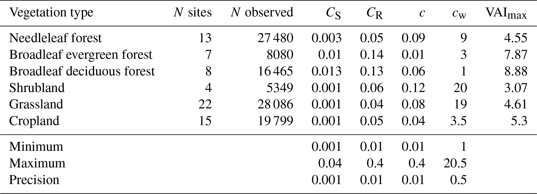
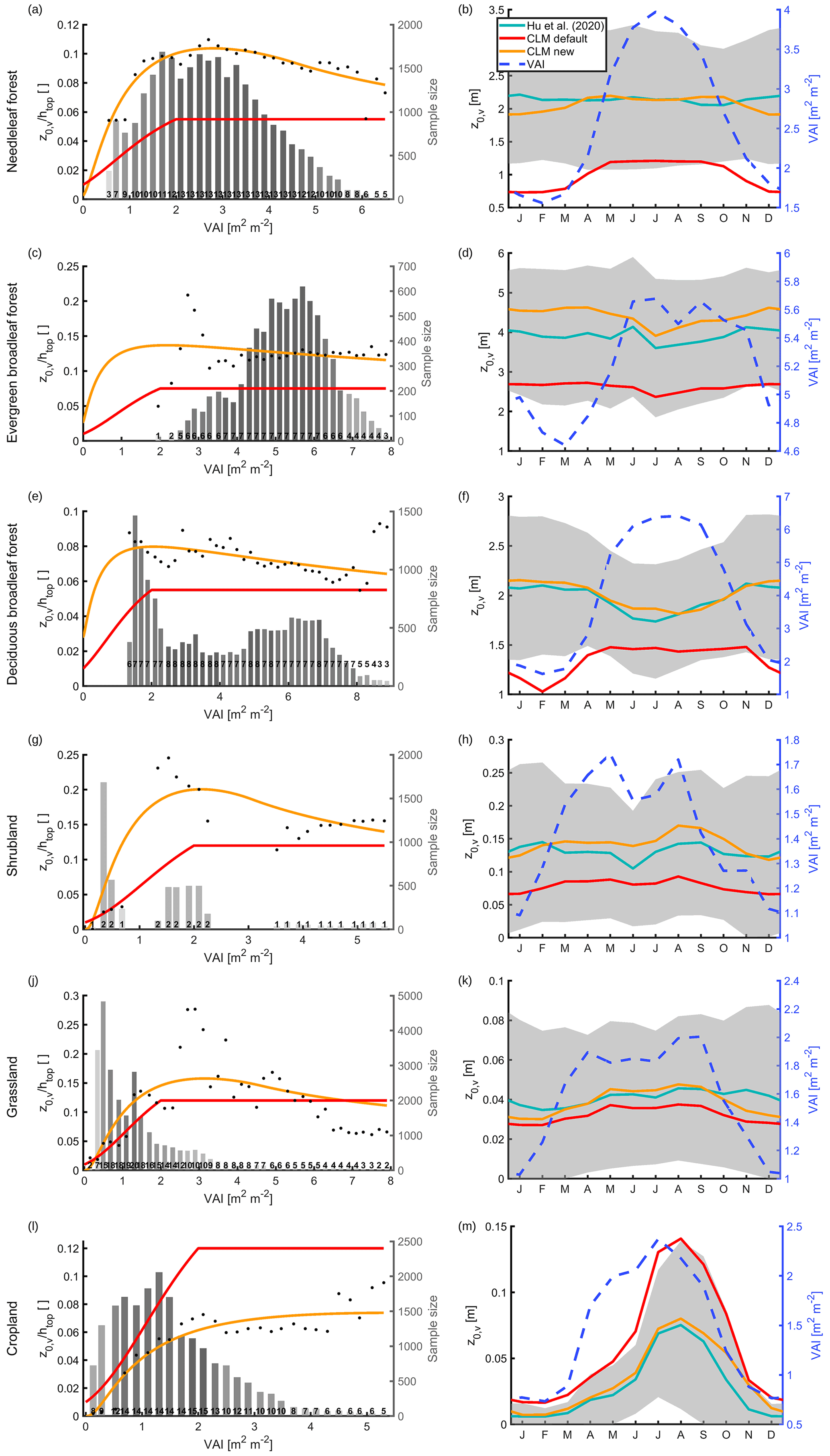
Figure 1 Left column: median $z_{\mathrm{0},\mathrm{v}}/h_{\mathrm{top}}$ of Hu20 in VAI bins as black dots, red line the default z_0,v parameterization of CLM, and orange line the optimized Ra92 parameterization. Height of gray bars shows the sample size in the respective bin and numbers at the bottom of the bars the number of sites that contributed to the respective bin. The darkness of the bars increases with an increasing fraction of total sites that are present in respective bin. Right column: monthly mean z_0,v in Hu20 (turquoise), with default parameterization of CLM (red) and with optimized Ra92 parameterization (orange). Gray shading shows mean of Hu20 ± 1 standard deviation and dotted blue line mean seasonal cycle of VAI. Note that the data of sites south of 30^∘ S were shifted by 6 months. (a–b) Needleleaf forests, (c–d) evergreen broadleaf forests, (e–f) deciduous broadleaf forests, (g–h) shrubland, (j–k) grassland, and (l–m) cropland.

2.3 Bare soil

CLM5 currently prescribes a z_0m,b of 0.01 m (Lawrence et al., 2018). As mentioned above, z_0h,b and z_0q,b differ from z_0m,b because scalar fluxes are not affected by the pressure fluctuations that are induced by the presence of the roughness elements. In CLM5, this is accounted for after Zeng and Dickinson (1998):

$$\begin{array}{}\text{(14)}& z_{\mathrm{0}\mathrm{h},\mathrm{b}}=z_{\mathrm{0}\mathrm{q},\mathrm{b}}=z_{\mathrm{0}\mathrm{m},\mathrm{b}}{e}^{-a(u_{*}{z}_{\mathrm{0}\mathrm{m}}/\mathit{\nu }{)}^{\mathrm{0.45}}},\end{array}$$

where a=0.13 and ν is the kinematic viscosity of air ($=\mathrm{1.5}\times {\mathrm{10}}^{-\mathrm{5}}$ m² s⁻¹). Note that this equation is also used to compute z_0h and z_0q over snow and ice.

Observed z_0m values over bare soil exhibit a wide range from $\mathrm{1}\times {\mathrm{10}}^{-\mathrm{5}}$ m to $\mathrm{1}\times {\mathrm{10}}^{-\mathrm{2}}$ m but are frequently around 0.001 m (Greeley et al., 1997; Callot et al., 2000; Marticorena et al., 2004, 2006; Hugenholtz et al., 2013; Nield et al., 2013). The default value of 0.01 m is within the observed range but lies at the upper end of it. To better determine the distribution of observed values, we synthesize z_0m,b observed values reported in the literature (Fig. 2). Specifically, we use the data compiled in Table 1 of Prigent et al. (2005), sites S8 and S9 in Table 6, as well as the data compiled in Table 7 of Marticorena et al. (2006), and the reported values in Hugenholtz et al. (2013) and Nield et al. (2013), making sure that no value is counted twice. When a range is reported, we compute the average of this range (e.g., 0.001–0.005 m would be included as 0.003 m). We confirm that the 0.01 m value used in CLM is near the maximum among the observations from the literature (Fig. 2). Therefore, we replace the current value with the median value from our literature synthesis ($\mathrm{8.5}\times {\mathrm{10}}^{-\mathrm{4}}$ m).

Several remote-sensing-based data sets exist for z_0m,b, which could potentially be used as an alternative to using one globally constant z_0m,b value (e.g., Marticorena et al., 2004; Prigent et al., 2005, 2012; Stilla et al., 2020). We therefore additionally implement the input of a spatially explicit z_0m,b based on the data of Prigent et al. (2005), which we subsequently refer to as Pr05. Unlike other data sets, Pr05 also covers warm deserts other than the Sahara. Pr05 employs observations of the backscattering coefficient from the European Remote Sensing Satellite (ERS) scatterometer, calibrated on quality in situ and geomorphological z_0m,b estimates, to derive monthly mean z_0m,b in arid and semi-arid regions for an equal-area grid of 0.25^∘ resolution at the Equator. To derive a spatially continuous input field for CLM, we collect the monthly data from all grid cells in Pr05 that fall within a focal grid cell in our simulations. We use the 25th percentile of the corresponding monthly data that fall within the focal grid cell as a temporally constant input for our simulations assuming that the temporal evolution in Pr05 results purely from the seasonality of vegetation (which is represented by the vegetation patches described in the previous section). The 25th percentile is chosen because vegetation normally exhibits a higher z_0m than the ground. For grid cells without observations in Pr05 we use the area-weighted global mean of all the grid cells that contain data ($\mathrm{4.1}\times {\mathrm{10}}^{-\mathrm{4}}$ m). We replace values of z_0m,b that fall below $\mathrm{1}\times {\mathrm{10}}^{-\mathrm{4}}$ m with this value for numerical stability. The z_0m,b values in Pr05 are at the lower side of in situ observations with values as low as $\mathrm{1}\times {\mathrm{10}}^{-\mathrm{5}}$ m. This might originate from the fact that Pr05 focuses on desert regions by excluding z_0m,b values above $\mathrm{8}\times {\mathrm{10}}^{-\mathrm{4}}$ m, while some in situ sites might exhibit a locally higher z_0m,b due to the presence of rocks or sparse vegetation elements.

Figure 2 Boxplot of the decimal logarithm in in situ observations of z_0m,b (left), z_0m,s (second from right), and z_0m,i (right). The value of n corresponds to the number of sites. Second boxplot from left shows z_0m,b in remote-sensing-based data of Prigent et al. (2005). Stars correspond to outliers, which are more than 1.5 times the interquartile range away from the box. Red dots show the current value in CLM5.

Next, we focus on the formulation of z_0h,b and z_0q,b. Yang et al. (2008) assessed the performance of seven different parameterizations for the ratio of $z_{\mathrm{0}\mathrm{h},\mathrm{b}}/z_{\mathrm{0}\mathrm{m},\mathrm{b}}$, including Eq. (14), at several bare soil sites. The formulations of Owen and Thomson (1963) and a revised version of Yang et al. (2002) performed best among the tested parameterizations. Further, $z_{\mathrm{0}\mathrm{h},\mathrm{b}}/z_{\mathrm{0}\mathrm{m},\mathrm{b}}$ exhibits distinct diurnal variations, which is reproduced best by the latter parameterization. The parameterization of Zeng and Dickinson (1998), on the other hand, overestimates $z_{\mathrm{0}\mathrm{h},\mathrm{b}}/z_{\mathrm{0}\mathrm{m},\mathrm{b}}$ strongly, particularly during the day. Similarly, Chen et al. (2010) implemented and tested several parameterizations of $z_{\mathrm{0}\mathrm{h},\mathrm{b}}/z_{\mathrm{0}\mathrm{m},\mathrm{b}}$ in the Noah LSM, confirming the good performance of the formulation proposed in Yang et al. (2008), which is subsequently called Ya08. In particular, the Ya08 parameterization reduced the underestimation of daytime LSTs of Noah in arid regions (Chen et al., 2011). Similar biases to those for Noah exist in CLM3.5, which could be improved by decreasing $z_{\mathrm{0}\mathrm{h},\mathrm{b}}/z_{\mathrm{0}\mathrm{m},\mathrm{b}}$ (Zeng et al., 2012).

Overall, there is clear evidence that the parameterization of z_0h,b and most likely also z_0q,b applied currently in CLM5 is in disagreement with observations. We therefore employ Ya08 for the parameterization of z_0h,b and z_0q,b:

$$\begin{array}{}\text{(15)}& z_{\mathrm{0}\mathrm{h},\mathrm{b}}=z_{\mathrm{0}\mathrm{q},\mathrm{b}}=(\mathrm{70}\mathit{\nu }/u_{*})\times \exp (-\mathit{\beta }{u}_{*}^{\mathrm{0.5}}|T_{*}{|}^{\mathrm{0.25}}).\end{array}$$

Here, β=7.2 and T_* is the frictional temperature defined as $-\text{SH}/\left(\mathit{\rho }{c}_p{u}_{*}\right)$, where SH is the sensible heat flux, ρ is the air density, and c_p is the specific heat of air at constant pressure. We have also tested the formulation of $z_{\mathrm{0}\mathrm{h},\mathrm{b}}/z_{\mathrm{0}\mathrm{m},\mathrm{b}}$ after Owen and Thomson (1963) in CLM and found no major difference to the model version using Ya08. Ya08 is also used in the revised version of CLM to compute the z_0h and z_0q of snow and ice, which will be described in more detail in the next two sections.

2.4 Snow

The current z₀ representation for snow is similar to the one of bare soil except that a globally constant z_0m,s value of 0.0024 m is used instead of 0.01 m. We here focus on z_0m,s, as the modifications of z_0h,s and z_0q,s were described in the previous section. For a comparison of z_0m,s, we collect the data compiled and measured with the wind profile method for snow in Brock et al. (2006) as well as the measured values in Fitzpatrick et al. (2019) and van Tiggelen et al. (2021), applying the same procedure for reported ranges as for bare soil. Again, the default value of 0.0024 m lies in the higher range of observed values, although less drastically than for bare soil (Fig. 2). Therefore, we replace the globally constant value for z_0m,s with the median value from the literature synthesis ($\mathrm{7.75}\times {\mathrm{10}}^{-\mathrm{4}}$ m).

Field observations show that z_0m,s increases as snow melting proceeds due to the formation of melting ponds (Brock et al., 2006; Fitzpatrick et al., 2019). Brock et al. (2006) propose the following parameterization of z_0m,s as a function of accumulated snowmelt to account for this relationship (solid line in Fig. 3):

$$\begin{array}{}\text{(16)}& \ln \left(z_{\mathrm{0}\mathrm{m},\mathrm{s}}\right)=b_{\mathrm{1}}\left\{\text{atan}\left(\left[{\log }_{\mathrm{10}}\left(M_{\mathrm{a}}\right)+\mathrm{0.23}\right]/\mathrm{0.08}\right)\right\}+b_{\mathrm{4}},\end{array}$$

where ln (z_0m,s) is the natural logarithm of z_0m,s in millimeters, b₁ and b₂ are empirical constants, and M_a is the accumulated snowmelt in meters water equivalent. For application in CLM, we compute the constants b₁ and b₂ such that the parameterization will pass through the 10th percentile of the data displayed in Fig. 2 as M_a=0 m and approaches the 90th percentile as M_a goes towards infinity, arriving at b₁=1.4 and $b_{\mathrm{4}}=-\mathrm{0.31}$ (dashed line in Fig. 3). M_a should decrease when fresh snow falls on snow that was previously melting. Therefore, we update M_a for snow that already existed at the previous time step as follows:

$$\begin{array}{}\text{(17)}& M_{\mathrm{a}}^t=M_{\mathrm{a}}^{t-\mathrm{1}}-Q_{\mathrm{snowfall}}^t+Q_{\mathrm{snowmelt}}^t,\end{array}$$

where $M_{\mathrm{a}}^t$ and $M_{\mathrm{a}}^{t-\mathrm{1}}$ are the accumulated snowmelt at the current time step and previous time step, respectively, $Q_{\mathrm{snowfall}}^t$ is the freshly fallen snow, and $Q_{\mathrm{snowmelt}}^t$ is the melted snow, all in meters water equivalent.

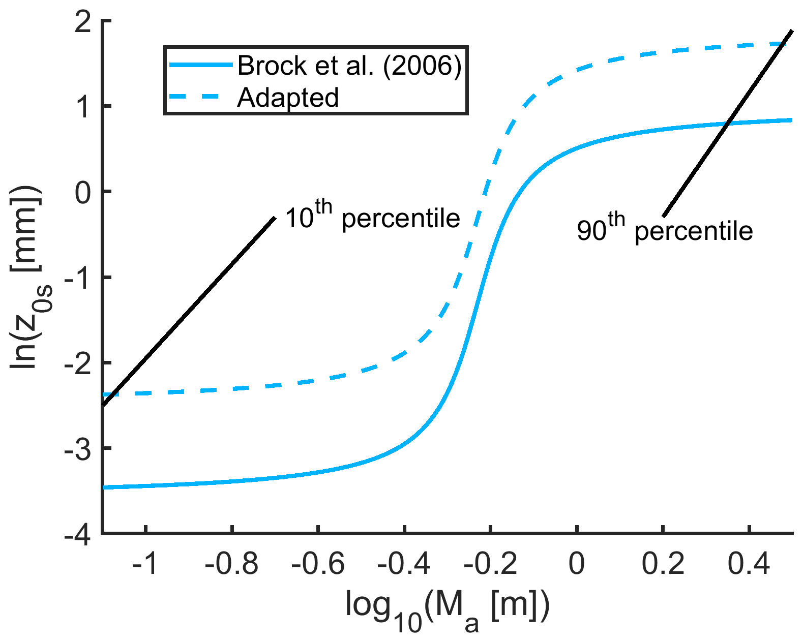
Figure 3 Parameterization of z_0m,s as a function of accumulated snowmelt since snowfall of Brock et al. (2006) (solid line) and parameterization with adapted constants, such that it passes through the 10th and 90th percentiles of data displayed in Fig. 2 (dashed line).

2.5 Glaciers

The surface roughness of ice sheets and glaciers is currently the same as that for bare soil in CLM. It should be noted that the surface properties of land ice play a somewhat subordinate role in CLM, since ice is generally covered by snow. As with snow, we employ the z_0m,i observations of Brock et al. (2006), Fitzpatrick et al. (2019), and van Tiggelen et al. (2021) for a comparison to CLM (Fig. 2). The z_0m of land ice tends to be higher than for bare soil or snow. Still, the current value of 0.01 m in CLM is on the upper end of the synthesized field observations. Accordingly, we decrease this globally constant value to $\mathrm{2.3}\times {\mathrm{10}}^{-\mathrm{3}}$ m, the median among the collected field observations.

2.6 Lakes

The current lake model in CLM, the Lake, Ice, Snow, and Sediment Simulator (LISSS), was developed by Subin et al. (2012). The z₀ parameterization for frozen (potentially snow-covered) lakes is the same as for ice and snow on land. However, the z_0m,i was decreased in the lake model to 0.001 m. For unfrozen lakes, z_0m, z_0h, and z_0q is parameterized as follows:

$$\begin{array}{}\text{(18)}& {\displaystyle }{z}_{\mathrm{0}\mathrm{m}}=max\left({\displaystyle \frac{\mathit{\alpha }\mathit{\nu }}{u_{*}}},{\displaystyle \frac{c{u}_{*}^{\mathrm{2}}}{g}}\right),\text{(19)}& {\displaystyle }{z}_{\mathrm{0}\mathrm{h}}=z_{\mathrm{0}\mathrm{m}}\exp \left(-{\displaystyle \frac{\mathit{\kappa }}{\mathit{Pr}}}\left(\mathrm{4}\sqrt{R_{\mathrm{0}}}-\mathrm{3.2}\right)\right),\end{array}$$

and

$$\begin{array}{}\text{(20)}& z_{\mathrm{0}\mathrm{q}}=z_{\mathrm{0}\mathrm{m}}\exp \left(-{\displaystyle \frac{\mathit{\kappa }}{\mathit{Sc}}}\left(\mathrm{4}\sqrt{R_{\mathrm{0}}}-\mathrm{4.2}\right)\right),\end{array}$$

where α=0.1, c is the effective Charnock coefficient (for details check Lawrence et al., 2018), g is the acceleration of gravity, Pr=0.71 is the molecular Prandt number for air, R₀ is the near-surface atmospheric roughness Reynolds number, and Sc=0.66 is the molecular Schmidt number for water in air. The resultant z_0m values over open water lie typically in the range of $\mathrm{1}\times {\mathrm{10}}^{-\mathrm{4}}$ to $\mathrm{5}\times {\mathrm{10}}^{-\mathrm{4}}$ m.

Subin et al. (2012) demonstrated the added value of the z₀ formulations described above compared to prescribing a constant value in LISSS. The WRF lake model also profited from an introduction of this parameterization (Xu et al., 2016; Wang et al., 2019). Li et al. (2015) find the dependence of z_0m, z_0h, and z_0q on wind speed in LISSS is not ideal for a lake over the Tibetan Plateau. However, the simulated values are generally of reasonable magnitude compared to the observed values. We conclude that there is no clear evidence for a need to revise the z₀ parameterization of LISSS. Therefore, we retain the current formulations for z₀ over lakes. We do, however, adopt the revisions for the z₀ of frozen lakes, consistent with the modifications for snow and ice on land described in Sect. 2.4 and 2.5.

2.7 Urban areas

In the urban module of CLM, z₀ and d are parameterized after Macdonald et al. (1998) as a function of the canyon height, H, the plan area index, λ_p, and the frontal area index λ_f (for more details see Oleson et al., 2008, 2010):

$$\begin{array}{}\text{(21)}& d=H\left(\mathrm{1}+{\mathit{\alpha }}^{-{\mathit{\lambda }}_{\mathrm{p}}}({\mathit{\lambda }}_{\mathrm{p}}-\mathrm{1})\right),\end{array}$$

and

$$\begin{array}{}\text{(22)}& z_{\mathrm{0}}=H\left(\mathrm{1}-{\displaystyle \frac{d}{H}}\right)\exp \left(-{\left[\mathrm{0.5}B{\displaystyle \frac{C_{\mathrm{D}}}{k^{\mathrm{2}}}}\left(\mathrm{1}-{\displaystyle \frac{d}{H}}\right){\mathit{\lambda }}_{\mathrm{f}}\right]}^{-\mathrm{0.5}}\right),\end{array}$$

where α=4.43 is an empirical coefficient and C_D is the depth-integrated mean drag coefficient for surface-mounted cubes in a shear flow. As for vegetation, this z₀ corresponds to the aerodynamic z₀ for the exchange between the urban canopy and the atmosphere. Again, there are additional resistance for the exchange of water vapor and energy between the surface of the different elements in the urban environment and the urban canopy air.

Variations of $z_{\mathrm{0}}/H$ among urban environments are considerable (e.g., Kanda et al., 2013). The parameterization of Macdonald et al. (1998) generally lies comfortably within the spread of $z_{\mathrm{0}}/H$ estimates (Grimmond and Oke, 1999; Nakayama et al., 2011; Kanda et al., 2013). We therefore conclude that there is no justification to revise the representation of z₀ and d in the urban module of CLM.

2.8 Resulting changes in surface roughness

Here, we present the impact on z₀ due to the proposed set of CLM modifications in land-only simulations, which will be described in the next section. The introduction of Ra92 leads to an increase in z_0,v for the forest PFTs (Fig. 4a and c). In particular, the z_0,v of forests increase by more than an order of magnitude during winter in some locations because the z_0,v of deciduous trees is raised considerably for low values of VAI (Fig. 1e). Changes in z_0,v for grassland and cropland PFTs generally exhibit no clear pattern, with the exception of a pronounced reduction in z_0,v in the northern high latitudes during winter (Fig. 4b and d).

The z_0m,g decreases by more than an order of magnitude in most regions due to the changes in z_0m,b, z_0m,s, and z_0m,i (Fig. 5a and d). In some coastal areas of Greenland, z_0m,g increases slightly, as enough snowmelt accumulates to reach the higher end of the Brock et al. (2006) parameterization for z_0m,s. The z_0h,g and z_0q,g now exhibit a distinct diurnal cycle following the introduction of Ya08. They decrease at daytime in low latitudes and during summer in the midlatitudes, while they increase under stable conditions that are often present in high latitudes and at night. In fact, the concurrent decrease of z_0m,g and increases of z_0h,g frequently result in a distinctly larger z_0h,g than z_0m,g (not shown). This is in contradiction to field observations, which normally find higher values of z_0m,g than for z_0h,g (Yang et al., 2002, 2008).

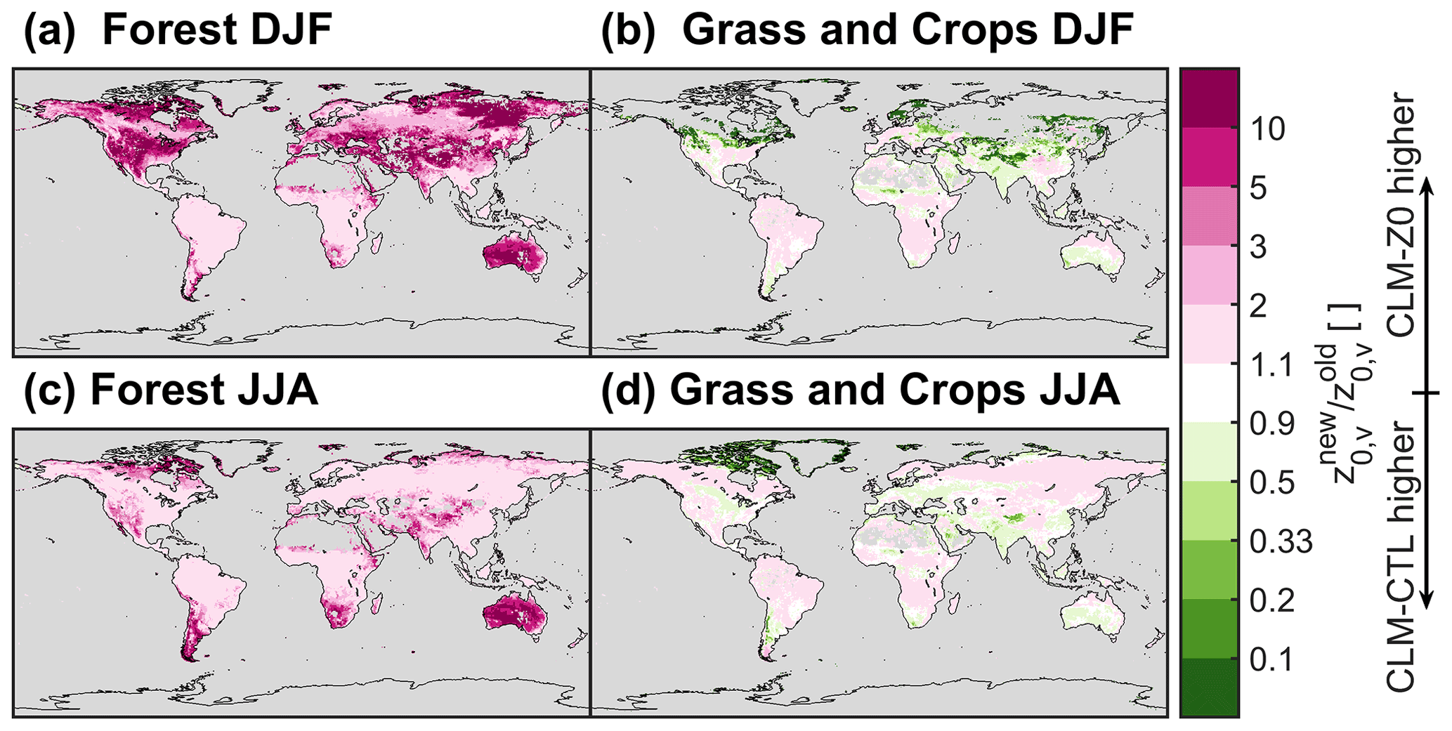
Figure 4 Ratio of new vegetation surface roughness (z_0,v; in CLM-Z0) divided by old z_0,v (in CLM-CTL). Panels (a) and (c) show the ratio of average z_0,v across forest plant functional types, and (b) and (d) show the ratio across grassland and cropland plant functional types. (a, b) Boreal winter (DJF) and (c, d) boreal summer (JJA). Data are masked if vegetation is buried completely by snow.

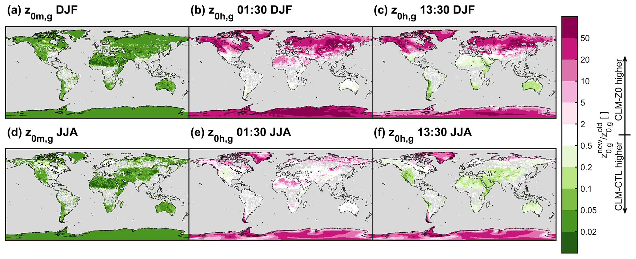
Figure 5 Ratio of new ground surface roughness (z_0,g) divided by old z_0,g. Panels (a) and (d) show the momentum surface roughness, (b) and (e) surface roughness of scalars at 01:30 local solar time, and (c) and (f) surface roughness of scalars at 13:30 local solar time. (a–c) Boreal winter (DJF) and (d–f) boreal summer (JJA).

3 Experiment design

We present results from two sets of simulations: (1) land-only simulations using CLM version 5.1 forced by the GSWP3 reanalysis data (Dirmeyer et al., 2006; Kim, 2014) and (2) land–atmosphere simulations with CESM version 2.1.2. For each simulation, we conduct a 50-year spinup followed by a 15-year analysis period using a near present-day climatological configuration. The vegetation phenology is prescribed from satellite observations in all simulations (SP mode in CLM). The different patches of vegetation are placed on separated soil columns to suppress lateral exchange of energy and water among them (Schultz et al., 2017; Meier et al., 2018) and biomass heat storage was activated to enable removal of the stability cap of the Monin–Obukhov stability parameter (Swenson et al., 2019; Meier et al., 2019). We additionally implement a new history file averaging flag that enables retrieval of model output at a specified local solar time. This allows us to determine the model state at a specific local solar time, for example at the time of MODIS LST observations at 01:30 and 13:30, without archiving data at all model time steps. For each configuration we conduct one control simulation with the existing representation of z₀ in CLM and a simulation in which we apply the updates for z₀ previously described.

For the CLM simulations, we use the component configuration set “I2000Clm51Sp”. These simulations are run at 0.5^∘ resolution. For the atmospheric forcing we cycle through the GSWP3 data of 1998–2012. The resulting simulations are called CLM-CTL and CLM-Z0 subsequently. In addition, a series of CLM land-only experiments are presented in Appendix A1 to assess the effect of the individual modifications. Table A1 provides an overview of all CLM simulations.

The CESM simulations are run in the configuration “F2000climo” at 0.9^∘ × 1.25^∘ resolution. This configuration couples CLM version 5.0 with the atmospheric model CAM version 6.0. The ocean is prescribed in F2000climo from the Hadley Centre Sea Ice and Sea Surface Temperature (HadISST) v1.1 data set (i.e., it is run in data mode; Hurrell et al., 2008). For the prescribed sea surface temperature forcing, we cycle through the data of 1998–2012 instead of using the data from 2000 only, as is normally the case in F2000climo. This is done to introduce more interannual variability. We refer to the CESM simulations as CESM-CTL and CESM-Z0.

4 Model analysis and evaluation

4.1 Reference data sets

We consult two observation-based data sets to assess the impact of the imposed modifications in CLM-Z0 and CESM-Z0 on model performance in terms of LST. First, we use observations of the MODIS system, which is installed on the low-Earth-orbit satellites, Terra and Aqua, to evaluate diurnal variations of the LST at grid cell level. These instruments provide LST estimates at a resolution of 1 km at approximately 01:30 and 13:30 local solar time at the Equator, based on the longwave radiation emitted by the land surface. We employ data from 2003–2012 of the product MYD11C3 version 6 (Wan et al., 2015), which has a native resolution of 0.05^∘. From these data, we compute a multi-year monthly climatology as described in Meier et al. (2019) at 0.5^∘ resolution. For comparison to the CESM simulations, we regrid this climatology to 0.9^∘ × 1.25^∘ with first-order conservative remapping of the Climate Data Operators (CDO) library. We output the LST in the model simulations at 01:30/13:30 and use only model output from 2003–2012 for a consistent comparison with MODIS. Further, we apply a cloud masking to the model output as described below.

In addition to comparing LST directly at grid cell level, we also evaluate the local LST difference between bare soil and vegetation. To extract such information from the MODIS LST observations, we repeat the space-for-time substitution approach as in Duveiller et al. (2018) to relate the LST to the land cover type. For the LST, we again employ monthly MYD11C3 data both at daytime (13:30) and during nighttime (01:30). The land cover fractions are based on the ESA Climate Change Initiative Land Cover project (ESA, 2017). We aggregate all land cover types that involve vegetation to form the vegetated land cover class, while we use the bare land class as bare soil. Then, we conduct a multiple linear regression between the MODIS LST observations and the land cover fractions within moving windows of 5 by 5 pixels for each month in 2008–2012 (see Duveiller et al., 2018, 2021, for details). The slope of this multiple linear regression between the vegetated land cover class and bare land forms the estimated LST sensitivity for a conversion between these two land cover types. With this procedure, we retrieve a monthly observation-based estimate of the LST sensitivity to a conversion of vegetation to bare soil at 0.25^∘ resolution, along with an estimate of the uncertainty associated with the regression. For comparison to the CLM simulations, we compute the multi-year monthly average at 0.5^∘ resolution, weighting all grid cells that fall into the focal location–month combination by area and by 1 over the uncertainty estimate of the respective value. The resultant reference data set is called Du18. In CLM, we compute the subgrid difference in the variable of interest of the bare soil patch minus all vegetation patches (including crops) within a grid cell as described in more detail in Meier et al. (2018). We only use cloud-masked LST data for 2008–2012, which was output at 01:30 and 13:30 local solar time.

4.2 Computation of LST and cloud masking

The LST in CLM is computed based on the leaf temperature (T_leaf) and the temperature of the ground (T_grnd):

$$\begin{array}{}\text{(23)}& \text{LST}=e_{\mathrm{v}}{T}_{\mathrm{leaf}}+(\mathrm{1}-e_{\mathrm{v}})T_{\mathrm{grnd}},\end{array}$$

where the vegetation emissivity, e_v, is a function of the VAI:

$$\begin{array}{}\text{(24)}& e_{\mathrm{v}}=\mathrm{1}-e^{-\mathrm{VAI}/\overline{\mathit{\mu }}}.\end{array}$$

Here, $\overline{\mathit{\mu }}$ corresponds to the average inverse optical depth for longwave radiation, which is set to 1 in CLM (Eq. 4.20 in Lawrence et al., 2018). T_grnd is a function of the snow temperature (T_snow), the temperature of the top soil layer (T_soil), the temperature of the surface water ($T_{{\mathrm{H}}_{\mathrm{2}}\mathrm{O}}$), the fraction of the ground covered by snow (f_snow), and the fraction of the ground covered by surface water ($f_{{\mathrm{H}}_{\mathrm{2}}\mathrm{O}}$):

$$\begin{array}{}\text{(25)}& \begin{array}{rl}{T}_{\mathrm{grnd}}& =\left[f_{\mathrm{snow}}(T_{\mathrm{snow}}{)}^{\mathrm{4}}+f_{{\mathrm{H}}_{\mathrm{2}}\mathrm{O}}(T_{{\mathrm{H}}_{\mathrm{2}}\mathrm{O}}{)}^{\mathrm{4}}\right.\\ & {\left.+(\mathrm{1}-f_{\mathrm{snow}}-f_{{\mathrm{H}}_{\mathrm{2}}\mathrm{O}})(T_{\mathrm{soil}}{)}^{\mathrm{4}}\right]}^{\mathrm{1}/\mathrm{4}}.\end{array}\end{array}$$

MODIS can observe the LST only under clear-sky conditions (Wan et al., 2015). We therefore remove cloudy conditions in our model output when confronting it with MODIS. For the CESM simulations, we can filter for clear-sky conditions directly from the total cloud cover model output. To do so, we output the total cloud coverage and the variables of interest at daily temporal resolution. In the postprocessing, we then remove days with an average total cloud coverage above 50 %. It is more complex to exclude cloudy days in the land-only CLM simulations, since the GSWP3 forcing does not include information on cloud coverage (Kim, 2014). We therefore mask for cloudy days based on the incoming shortwave radiation. This is done through a comparison to the daily incoming solar radiation at the top of the atmosphere according to Berger (1978), W_TOA, which is a function of latitude and the day of the year. However, solar radiation passing through the atmosphere can be altered even under clear-sky conditions, for example, because of aerosols (IPCC, 2013). Therefore, we derive a climatology of the incoming solar radiation at the surface under clear-sky conditions, $W_{\mathrm{S}}^{\mathrm{cs}}$, based on W_TOA in an iterative procedure:

1. A multiplicative factor, C, is optimized, such that it minimizes the sum-squared deviation to the daily incoming solar radiation forcing of GSWP3 at a given location:

   $$\begin{array}{}\text{(26)}& W_{\mathrm{S}}^{\mathrm{cs}}=C\cdot W_{\mathrm{TOA}}.\end{array}$$

2. Incoming solar radiation values below 80 % of $W_{\mathrm{S}}^{\mathrm{cs}}$ are removed for the next iteration, unless the current fit is based on less than 200 values (the iteration starts with $\mathrm{15}\cdot \mathrm{365}=\mathrm{5475}$ values).

3. This iteration is stopped if the sum-squared deviation of $W_{\mathrm{S}}^{\mathrm{cs}}$ to the remaining daily incoming solar radiation forcing of GSWP3 improves by less than 10 W² m⁻⁴.

With this procedure, we estimate $W_{\mathrm{S}}^{\mathrm{cs}}$ for each land point. We then remove days where the daily incoming solar radiation lies below 20 W m⁻² or below 90 % of $W_{\mathrm{S}}^{\mathrm{cs}}$ in the postprocessing of the model output of the CLM simulations. Figure 6 illustrates this clear-sky masking for four grid cells. Note that this cloud-masking procedure is not perfect because it effectively ignores clouds at night and does not distinguish between cloud types, which affect the incoming shortwave radiation at the surface differently (L'Ecuyer et al., 2019). Also, it results in data gaps during the polar night, because no incoming shortwave radiation is available for the cloud-masking procedure.

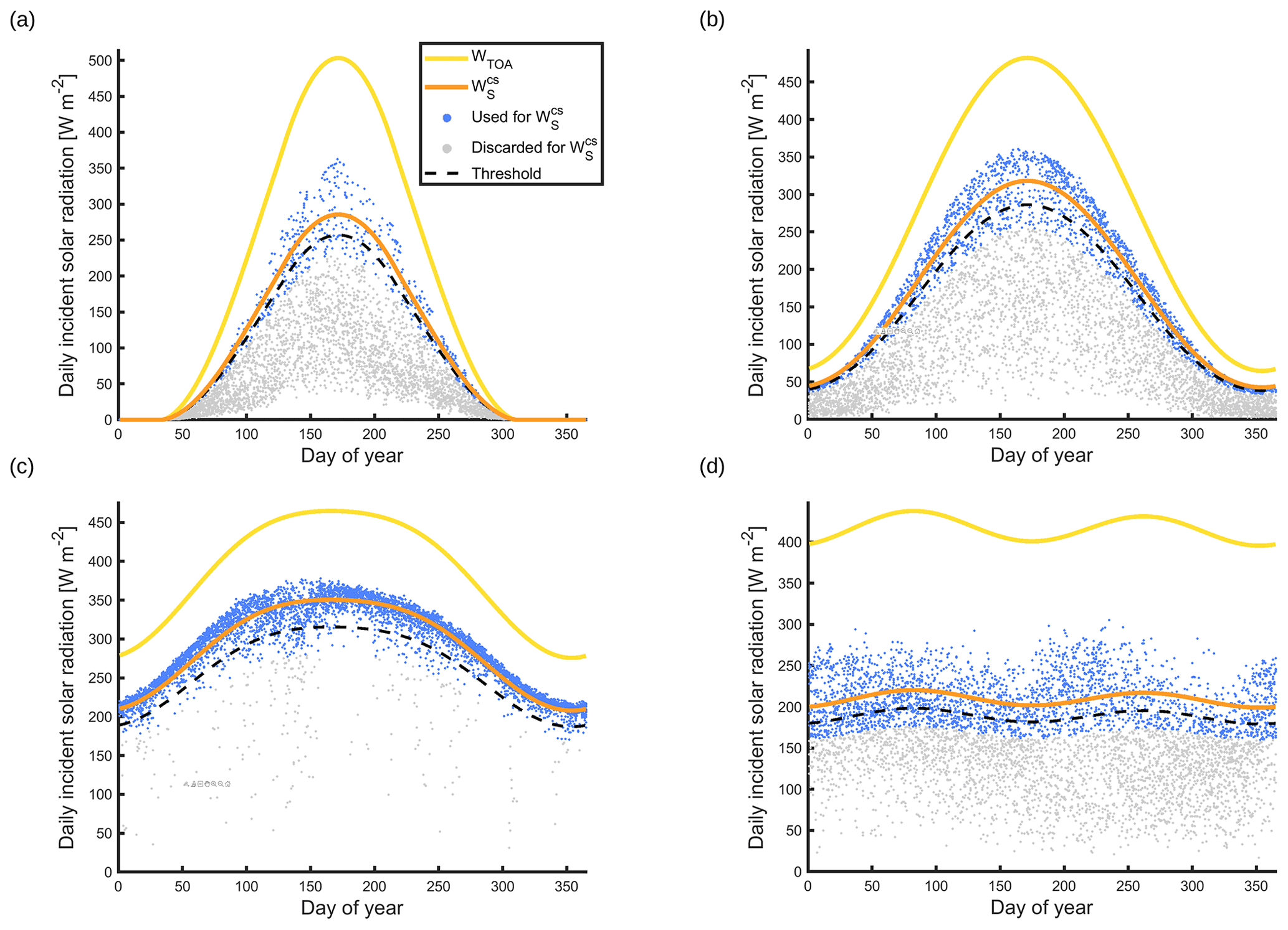
Figure 6 Examples of cloud masking based on incoming shortwave radiation at (a) 73.25^∘ N/11.75^∘ E, (b) 53.25^∘ N/11.75^∘ E, (c) 23.25^∘ N/11.75^∘ E, and (d) 3.25^∘ N/11.75^∘ E. The yellow line shows daily incoming solar radiation at the top of atmosphere according to Berger (1978), the orange line shows fitted incoming shortwave radiation at the surface under clear-sky conditions, the blue dots show daily incoming solar radiation values in GSWP3 included to make this fit, the gray points show daily incoming solar radiation values in GSWP3 removed because they are below 80 % of the last fit of $W_{\mathrm{S}}^{\mathrm{cs}}$, and the dashed black line shows the threshold of 90 % of $W_{\mathrm{S}}^{\mathrm{cs}}$ above which days are considered to have clear-sky conditions.

4.3 Significance testing

The CESM simulations exhibit a considerable degree of interannual variability. Therefore, we conduct a statistical test to assess whether the identified seasonal differences between CESM-Z0 and CESM-CTL are significant. First, we conduct a one-sample Student's t test at 5 % confidence level for the sample of seasonal mean differences between CESM-Z0 and CESM-CTL for each grid cell and season. This test in isolation is inappropriate when applied to a spatially autocorrelated field, as clustered areas can appear erroneously significant (Wilks, 2016). Thus, we control the false discovery rate as proposed in Wilks (2016) using a confidence level of 10 % ($=\mathrm{2}\cdot \mathrm{5}$ %), which is appropriate for data with a moderate to strong spatial autocorrelation. In addition, we include the last 30 years of the spinup period for some variables to corroborate the presented results.

5 Results

We first focus on the LST response at 01:30/13:30 local solar time in the land-only CLM simulations in Sect. 5.1. We also compare the simulated diurnal variations in LST to MODIS observation as well as the subgrid LST difference between bare soil and vegetation to Du18. In Sect. 5.2 we focus on the results from the CESM land–atmosphere simulations. Initially, the focus is again on the LST (Sect. 5.2.1) and additionally the air temperature at the bottom of the atmosphere (Sect. 5.2.2). Afterwards, we present alterations in wind speed. Note that we present a number of sensitivity experiments in Appendix A1, where we assess the influence of the different z₀ modifications individually. Further, we conduct an energy balance decomposition after Luyssaert et al. (2014) in Appendix A2 to link the changes in LST described in this section to individual energy fluxes.

5.1 LST response in land-only simulations

At 13:30, the LST increases substantially in warm desert regions (Fig. 7a and c). This warming originates mainly from the reduction in z_0m,g, while the introduction of the Ya08 formulation for z_0h,g and z_0q,g produces only a small impact (Appendix A1). The reduced z_0m,g inhibits the exchange of sensible heat with the atmosphere (Fig. A2). The solar radiation absorbed by the land surface in desert regions is therefore transferred less efficiently to the atmosphere in CLM-Z0. Consequently, the land surface warms and maintains its energy balance through emission of more longwave radiation and a higher ground heat flux (Fig. A2). Accordingly, the induced warming is higher during the summer season, when the solar irradiance is highest. On the other hand, the reduction in z_0m,g decreases the LST in the cold deserts, in particular during the winter season. This is again the result of a reduced sensible heat flux, which is however generally directed from the warmer atmosphere to the land surface in those regions. In vegetated areas, the increased z_0,v of forests enhances the turbulent transport of energy away from the land surface (Fig. A2), producing a cooling of the daytime LST.

The LST response at 01:30 is generally considerably weaker than the daytime effect (Fig. 7b and d). Conditions in the surface layer are more commonly stable at night, inhibiting the turbulent energy exchange between the land and the atmosphere. Also, there is no strong energy input to the land surface in the form shortwave radiation at night. Therefore, our modifications of z₀ produce a weaker effect. Interestingly, the pronounced daytime warming effect in the warm deserts translates into the night through the energy stored in the soils (Fig. A3). In contrast, the increase in z_0,v of forests warms the land surface at night in particular during summer by increasing the sensible heat flux towards the land. Thus, the LST response at 01:30 over vegetation opposes the daytime response in sign, unlike in desert regions. This is likely the case, because the LST in CLM is linked tightly to the leaf temperature, which exhibits a smaller thermal inertia than the ground (Eq. 23). Consequently, the alterations in LST change sign diurnally in regions dominated by vegetation, while the sign remains the same over regions dominated by bare soil.

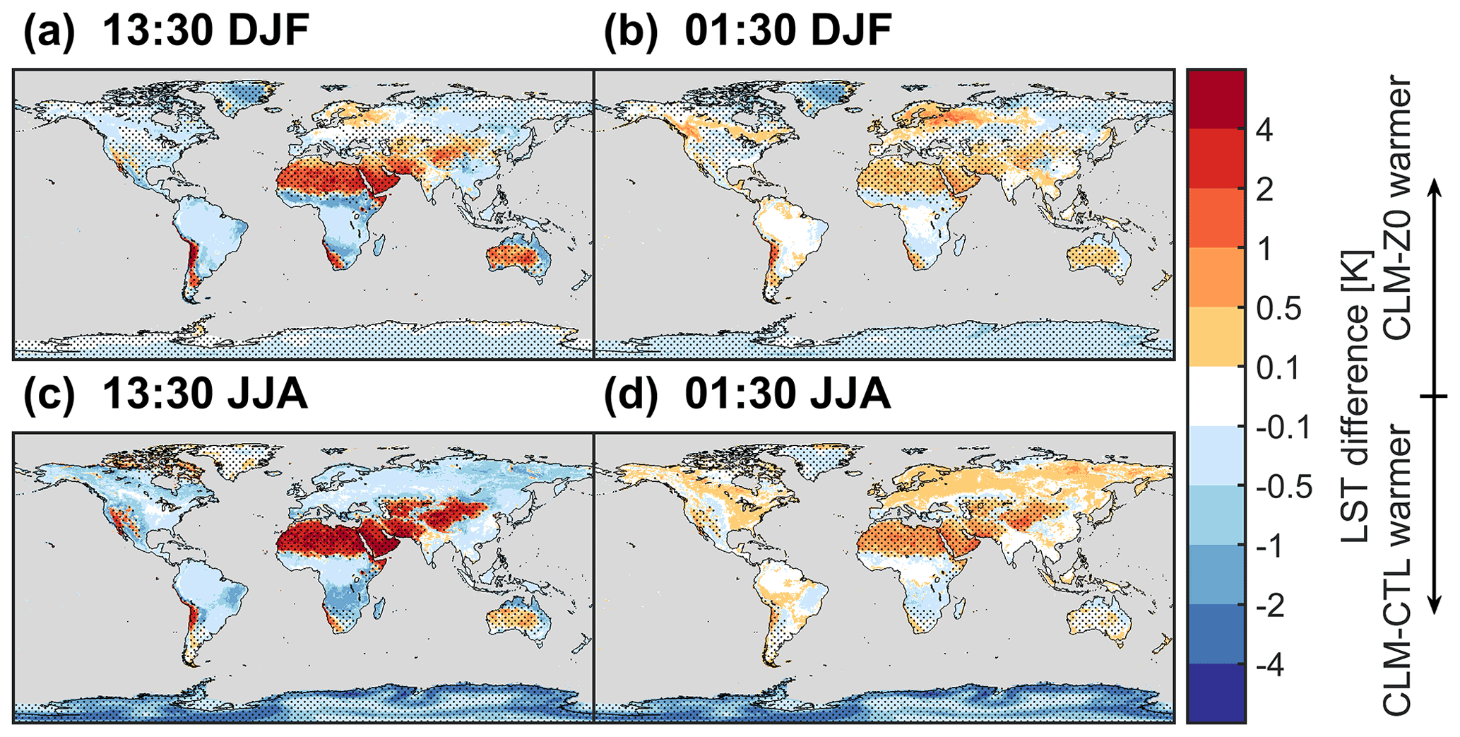
Figure 7 LST difference between CLM-Z0 and CLM-CTL. (a, c) LST difference at 13:30 local solar time and (b, d) difference at 01:30 local solar time. (a, b) Boreal winter (DJF) and (c, d) boreal summer (JJA). The stippling shows areas dominated by bare soil with a seasonal average VAI below 0.5 m² m⁻². Note the non-linear color scale.

Overall, the modified z₀ amplifies the diurnal temperature range (DTR; here defined as the LST difference between 13:30 and 01:30 local solar time) in desert regions and dampens the DTR in regions with forests (Fig. 8a). This links back to previous studies that found an overestimation of the DTR in desert regions and an underestimation over forests in CLM compared to remote sensing observations (Zeng et al., 2012; Meier et al., 2019). This tendency prevails in the current version (5.1) of CLM (Fig. 8d). The modifications of z₀ in CLM-Z0 alleviate these biases in most regions with the notable exception of the southern half of the Sahara, where the reduced z_0m,g in CLM-Z0 frequently overcompensates an only slight underestimation of the LST DTR in CLM-CTL (Fig. 8b, c, e, and f).

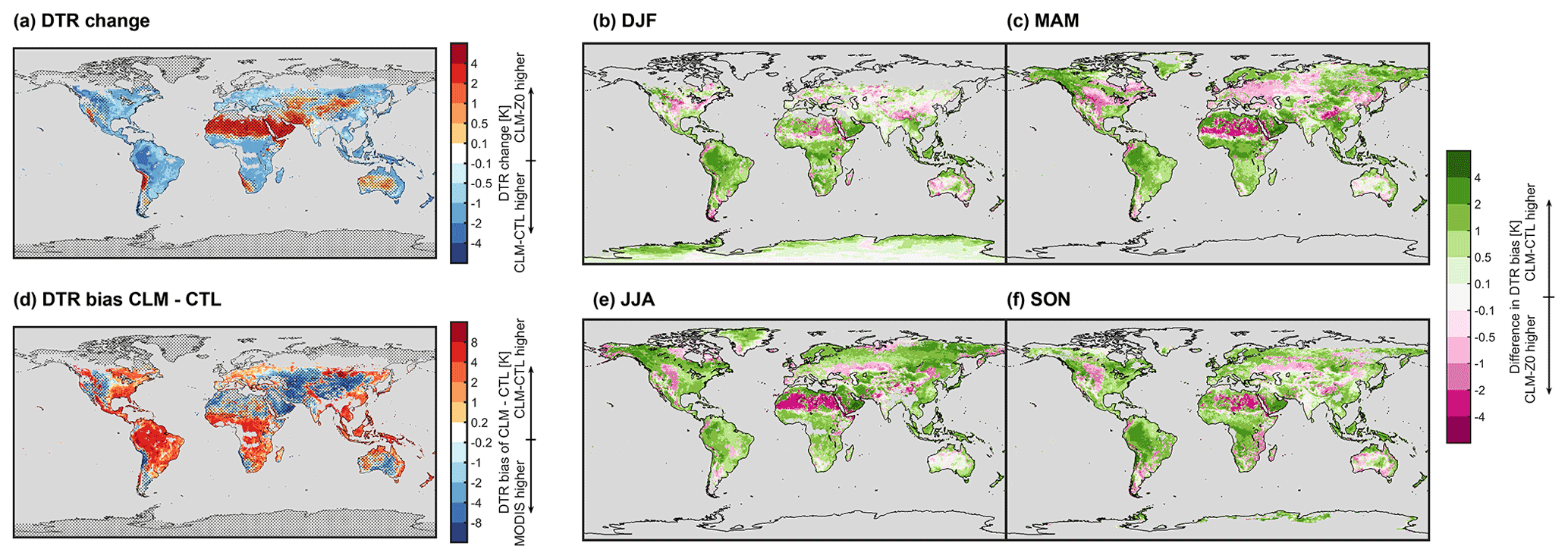
Figure 8 Panel (a) shows the difference in LST DTR of CLM-Z0 minus CLM-CTL and panel (d) bias in LST DTR of CLM-CTL compared to MODIS remote sensing observations. The stippling in those panels shows areas with an average VAI below 0.5 m² m⁻². To the right, the changes in the LST DTR bias between CLM-Z0 and CLM-CTL in boreal winter (b), spring (c), summer (e), and autumn (d) are shown. CLM data are cloud masked based on the incoming shortwave radiation. Note the non-linear color scale.

The modifications in CLM-Z0 also affect the sensitivity of the LST to land cover. Here, we compare the LST response to a conversion of vegetated land to bare soil, as estimated in Du18, to the subgrid LST difference between the vegetated tiles and the bare soil tiles in CLM. This land cover transition is likely relevant for the biogeophysical response to desertification, which has become more common over the last decades (IPCC, 2019). Overall, Du18 observes an increase in LST at 13:30 over bare soils compared to vegetation with the exception of latitudes exceeding 40^∘ N/S during the colder months (Fig. 9a). CLM-CTL exhibits a lower daytime LST over bare soil tiles than over vegetated tiles in most regions (Fig. 9b). CLM-Z0 captures the LST increase for a conversion of vegetation to bare soil at 13:30 in most cases (Fig. 9c). However, the signal is considerably stronger than in Du18, resulting in a higher RMSE for this simulation than in CLM-CTL. At night, the modifications in CLM-Z0 further amplify a positive bias in the LST difference between bare soil and vegetation in CLM-CTL in comparison to Du18 (Fig. 9e–h). For the DTR, Du18 finds an amplification over bare land compared to vegetation for most latitude–month combinations, with the exception of the high latitudes during winter (Fig. 9j). CLM-CTL on the other hand mostly exhibits a lower DTR over bare soil than over vegetation (Fig. 9k). This bias is mitigated to some extent in CLM-Z0, even though a dampening of the DTR often persists in the northern midlatitudes (Fig. 9l). Overall, the imposed alterations in z₀ do not result in a clear and consistent improvement of the LST response to a conversion between vegetation and bare soil but clearly do alter this sensitivity. Some discrepancies between Du18 and the CLM simulations might also arise from the absence of atmospheric feedbacks in the subgrid approach, which are used to diagnose the land cover sensitivity in CLM (note that the subgrid approach would still neglected atmospheric feedbacks in the CESM simulations; for more information see Chen and Dirmeyer, 2020). In addition, the cloud masking based on the incoming solar radiation could potentially introduce mismatches between CLM and Du18, in particular at night. Further, preferential occurrence of clouds over vegetation or bare soil could introduce biases in Du18. In fact, a recent study observed increased low-level cloud cover over forests compared to short vegetation, using a similar methodology as in Du18 (Duveiller et al., 2021).

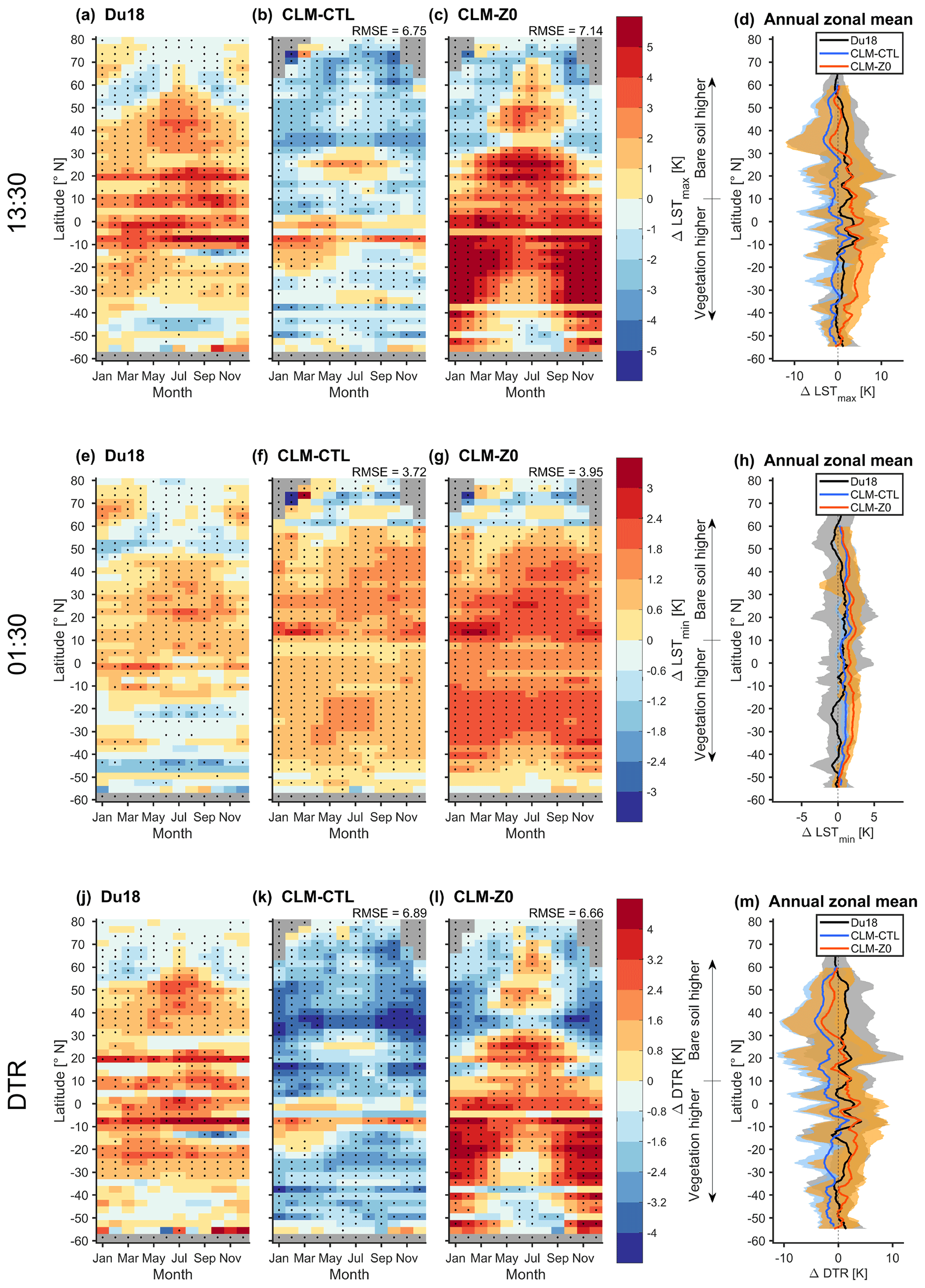
Figure 9 LST sensitivity in Du18 and CLM to conversion of vegetation to bare land. (a–d) LST difference between bare soil minus vegetated land at 13:30 local solar time (ΔLST_max). Seasonal and latitudinal variations of (ΔLST_max) in (a) the observation-based estimate of Du18, (b) CLM-CTL, and (c) CLM-Z0. Points with a mean which is significantly different from 0 in a two-sided t test at the 95 % confidence level are marked with a black dot. All data from the 2008–2012 analysis period corresponding to a given latitude and a given month are pooled to derive the sample set for the test. The numbers next to the titles are the area-weighted spatiotemporal root-mean-squared deviation of the respective simulation against Du18. Panel (d) shows the zonal annual mean of Du18 (black, range between the 10th and 90th percentiles in gray), CLM-CTL (blue, range between the 10th and 90th percentiles in blue), and CLM-Z0 (red, range between the 10th and 90th percentiles in orange). Note that on this subfigure results have been smoothed latitudinally with a simple moving average over 4^∘. CLM data are cloud masked based on the incoming shortwave radiation. Panels (e–h) are the same for the LST difference at 01:30 local solar time and panels (j–m) for the diurnal temperature range.

5.2 Effect in land–atmosphere coupled simulations

In the preceding section, we assessed the impact of the proposed changes to z₀ in land-only simulations. However, the resultant changes in land turbulent fluxes may also affect the atmosphere. In this section, we therefore evaluate the impact of the z₀ modifications in land–atmosphere simulations.

5.2.1 LST response

At low latitudes, the LST at 13:30 in CESM-Z0 increases over the deserts and decreases in most regions with dense vegetation, similar to the land-only simulations (Fig. 10a and b). However, the daytime warming in deserts is stronger in the coupled simulations (Fig. 7). It therefore appears that atmospheric feedbacks trigger an additional warming of the land in these regions. Indeed, we find an increase in incoming shortwave radiation accompanied by a reduction in cloud cover, which is most notable over the Sahara and the Middle East (Fig. 10e–h and Figs. A4 and A1). Previous studies have found that an increase in the sensible heat flux favors cloud coverage (Khanna et al., 2017; Bosman et al., 2019). It is therefore possible that the reduction in cloud coverage over desert regions in CESM-Z0 is a byproduct of the lower sensible heat flux in this simulation. Over the northern midlatitudes and high latitudes, an increase in cloud cover during summer coincides with a reduction in daytime LSTs due to less incoming shortwave radiation (Fig. A4). The LST response at night is often weaker but of the same sign as the daytime signal in CESM, similar to the land-only simulations (Fig. 10c and d). However, no distinct nighttime warming emerges over midlatitude forests during the summer season at night in the coupled simulations (compare Figs. 7d and 10d). In the mid- and high latitudes, changes in LST often exhibit a similar spatial pattern to surface air temperature changes, which are discussed in more detail in the next section (compare Figs. 10 and A6). In particular, the warming of the LST during winter over Alaska and western Canada appears to be related to more incoming longwave radiation at the surface (Fig. A1), which could be the result of warmer atmospheric temperatures in this region (Fig. A6a).

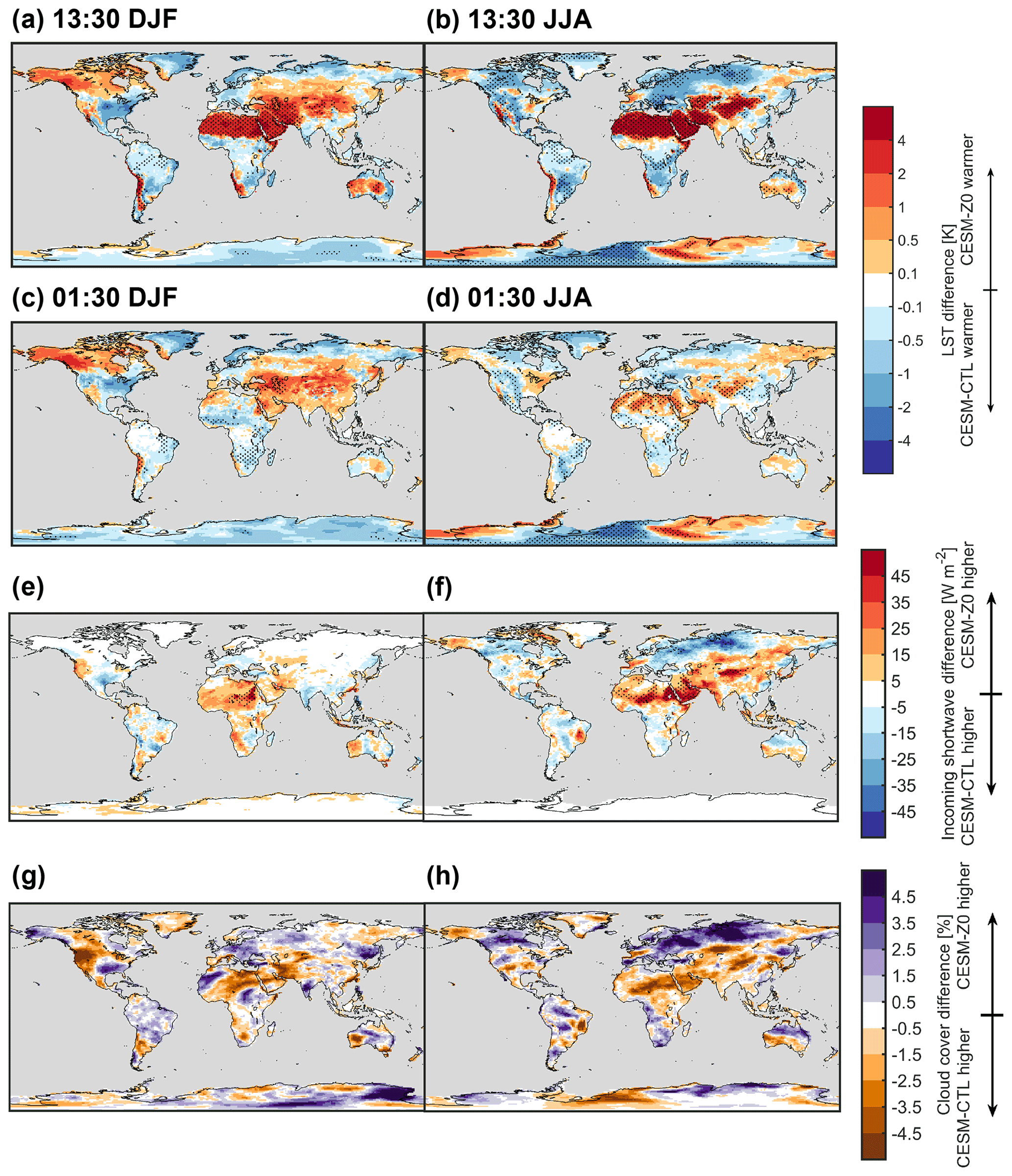
Figure 10 LST difference between CESM-Z0 and CESM-CTL at (a–b) 13:30 local solar time and (c–d) 01:30 local solar time. Panels (e) and (f) show the difference in incoming shortwave radiation at 13:30 local solar time between CESM-Z0 and CESM-CTL, and (g) and (h) show the difference in daily average total cloud cover. The stippling shows areas with a difference that is statistically significant different from 0 in a two-sided t test at the 95 % confidence level with a controlled false discovery rate. The left column shows boreal winter (DJF) and the right column boreal summer (JJA). Note the non-linear color scale for panels (a–d).

Compared to the MODIS observations, CESM-CTL underestimates the DTR over arid and semi-arid areas even more than CLM-CTL (Fig. 11d). On the other hand, the DTR is overestimated over most regions with dense vegetation and regions with permanent ice sheets. Again, the reduced z_0m,g amplifies the DTR in warm desert regions producing an improved agreement with the remote sensing observations (Fig. 11). Apart from these regions, the results are more mixed. Still, there is a clear improvement over the northern midlatitudes during boreal summer. Yet, the alterations of z₀ in CESM-Z0 do not entirely alleviate the existing biases in the LST DTR of CESM (Fig. A7). The remaining biases may not only originate from deficiencies in the land model itself but could also be related to atmospheric processes such as radiative transfer in the air column.

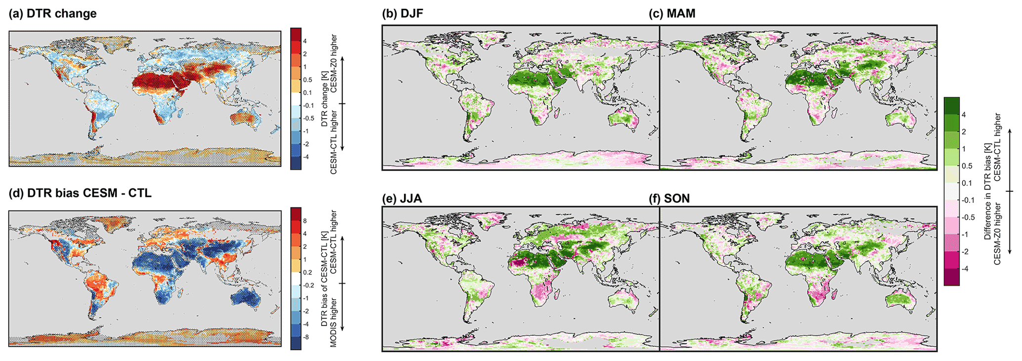
Figure 11 As Fig. 8 but for land–atmosphere coupled simulations CESM-Z0 and CESM-CTL. CESM data are cloud masked.

5.2.2 Response in surface air temperature and comparison to LST

The altered surface energy fluxes also affect air temperatures at the bottom of the atmospheric column (TBOT). The difference in daily average TBOT between CESM-Z0 and CESM-CTL exhibits considerable interannual variability. Therefore, we included the last 30 years of the spinup period to corroborate the results shown in Fig. 12a and b. Figure A6 depicts the average TBOT response for the analysis period and the last 30 years of the spinup period separately. Even when including these additional years, some pronounced features, such as the wintertime warming of average TBOT over north Asia, are still not statistically significant. Nevertheless, the wintertime average TBOT increases considerably in many regions in the Northern Hemisphere, showing a similar spatial pattern to that of the LST response (Fig. 12a). This is linked to more incoming longwave radiation (Fig. A1). On the other hand, the increase in z_0,v decreases the summertime TBOT in those regions (Fig. 12b). This can be explained by lower incoming shortwave radiation in CESM-Z0 compared to CESM-CTL (Fig. A4) as a result of higher total cloud coverage (Fig. 10e). Consequently, less energy is available close to the land surface in CESM-Z0, cooling both the LST and TBOT. At low latitudes, TBOT decreases mostly over the rainforests. Interestingly, CESM-Z0 also often exhibits a lower average TBOT over the Sahara in particular during boreal winter, thus opposing the LST response in sign. Further, there is a distinct band where TBOT warms in JJA over the Sahel region, while it cools both just north and south of this region (Fig. 12b).

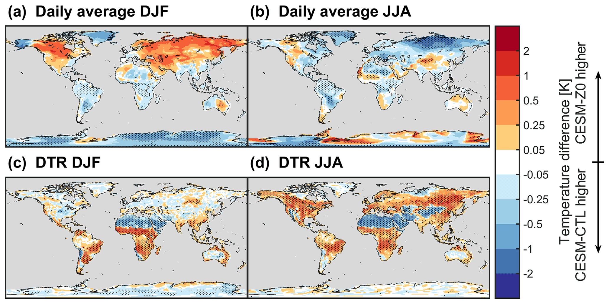
Figure 12 (a–b) Seasonal average difference in air temperature at the bottom of the atmospheric column (TBOT) between CESM-Z0 and CESM-CTL using data from the last 30 years of the spinup period and data from the analysis period (15 years). (c–d) Difference in TBOT DTR. The stippling shows areas with a difference that is statistically significant different from 0 in a two-sided t test at the 95 % confidence level with a controlled false discovery rate. (a, c) Boreal winter (DJF) and (b, d) boreal summer (JJA). Note the non-linear color scale.

The effect on the DTR of TBOT in CESM-Z0 opposes the effect on the LST DTR in sign, which is most visible in Africa (compare Fig. 12c and d to Fig. 11a). Where z₀ is decreased, less energy is transferred from the land into the atmosphere under unstable surface layer conditions (which are frequently present during day) and from the atmosphere to the land surface under stable conditions (frequently present at night). Consequently, the DTR at the land surface (LST) is amplified, while the DTR is dampened in the atmosphere above. This dipole between the DTR response of LST and TBOT to alterations in z₀ was previously found also in the context of deforestation in CESM (Chen and Dirmeyer, 2019) and in a number of regional climate models (Breil et al., 2020).

Figure 13 displays how the response of the DTR in LST and TBOT scale with the change in z_0m for latitudes between 30^∘ N/S. The DTR in LST for the individual vegetation patches decreases linearly with the logarithm of the ratio between the z_0,v in CESM-Z0 and the z_0,v in CESM-CTL $\left({\log }_{\mathrm{10}}(z_{\mathrm{0},\mathrm{v}}^{\mathrm{new}}/z_{\mathrm{0},\mathrm{v}}^{\mathrm{old}})\right)$, with a slope of −3 K (when using the decimal logarithm; Fig. 13a). In other words, a 10-fold increase in z_0,v dampens the LST DTR by 3 K. At grid cell level, the LST DTR exhibits a similar dependence on the change in z_0m between CESM-Z0 and CESM-CTL, if z_0m changes by no more than a factor of 3, as visible by values between −0.5 to 0.5 on the x axis in Fig. 13b. For stronger reductions in z_0m over desert regions the amplification of the LST DTR saturates at approximately 4 K (values below −0.5 on the x axis). It therefore appears that the distinct linear relation of the LST DTR to ${\log }_{\mathrm{10}}(z_{\mathrm{0},\mathrm{v}}^{\mathrm{new}}/z_{\mathrm{0},\mathrm{v}}^{\mathrm{old}})$ at PFT level does not hold at grid cell level for strong reductions in z_0m. This effect might originate from several factors. First, smaller changes in z_0m between CESM-Z0 and CESM-CTL occur over vegetation, while the strong reductions occur over bare soil (compare Figs. 4 to 5a and d). It might therefore be that the LST reacts more strongly to alterations of z_0,v than to alterations of z_0m,g due to the smaller thermal inertia of vegetation compared to soils. Second, different types of land cover with varying changes in z_0m are mixed at the grid cell level. For some PFT patches, z_0,v increases by more than an order of magnitude (i.e., ${\log }_{\mathrm{10}}(z_{\mathrm{0},\mathrm{v}}^{\mathrm{new}}/z_{\mathrm{0},\mathrm{v}}^{\mathrm{old}})>\mathrm{1}$), which is never the case for entire grid cells. We therefore cannot establish from our model experiments how the DTR would react to increases in z_0m by an order of magnitude at grid cell level. Third, our sensitivity experiments in Appendix A2 show that the reductions of z_0m,g in combination with the alterations z_0,v amplify the response of the LST DTR over vegetation, compared to a simulation were only z_0,v changed. And fourth, the sensitivity experiments indicate that the introduction of Ya08 for z_0h,g and z_0q,g moderates the effect of the decreased z_0m,g over the Sahara on the LST DTR.

Again, the dipole between the LST DTR response and the TBOT DTR response can be observed when comparing panels (b) and (c) in Fig. 13. The two variables are clearly mirrored in sign. However, the response in TBOT DTR is considerably weaker than the one of LST. This is likely owed to the differing nature of these two variables. The LST is computed from the temperatures of the leaves and the ground and is therefore tightly linked to the energy redistribution at the land surface. In contrast, TBOT is affected not only by the energy redistribution at the land surface but also by lateral and vertical mixing of air masses. This mixing may explain why the TBOT DTR response is generally weaker than the LST DTR response.

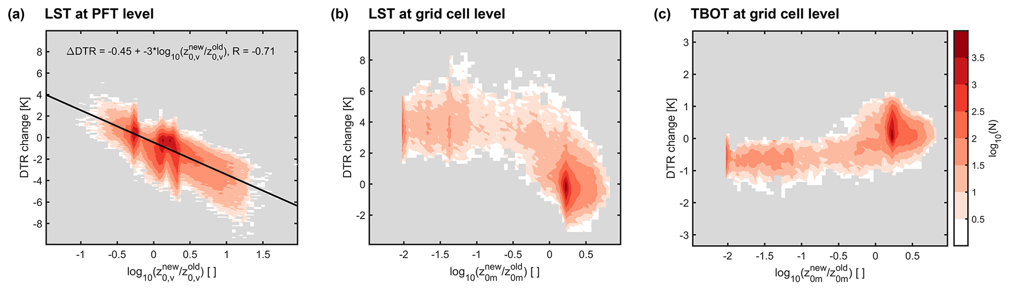
Figure 13 (a) Density plot of change in multi-year monthly mean LST DTR at the PFT level of CESM-Z0 minus CESM-CTL versus the decimal logarithm of the ratio of z_0,v in CESM-Z0 divided by z_0,v in CESM-CTL. Bin size on the x axis is 0.05, and on the y axis it is 0.1 K. Color scale on the far right shows the decimal logarithm of the number of tiles that fall within the respective bin. Multi-year monthly mean data of all PFTs excluding bare soil between 30^∘ N/S were used to generate this figure. (b–c) The same for the LST DTR (b) and TBOT DTR (c) at grid cell level and the maximum of z_0m,g and z_0,v. Bin size on the y axis in panel (c) is 0.05 K. The black line in panel (a) shows the linear fit with its formula and the Pearson correlation coefficient (R) above. Note the differing ranges of the y axis for the different panels.

5.2.3 Response of surface wind speed

The changes in z_0m affect the drag exerted by the land, and thus the wind speed, at least close to the land surface. The wind speed at the lowest atmospheric level increases notably in CESM-Z0 over desert regions, where z_0m was lowered, such as the Sahara, Greenland, or Antarctica (Fig. 14a and d). The remaining land mass is dominated by reductions in surface wind speed, consistent with the increases in z_0,v that were introduced for most vegetation types in CESM-Z0. These alterations of surface wind speed decay relatively abruptly with height and are only rarely significant at a height of 1.1 km (Fig. 14b and e). Even over the Sahara, where wind speeds close to the surface increase considerably, this signal disappears about 2.5 km above the surface (Fig. 14f).

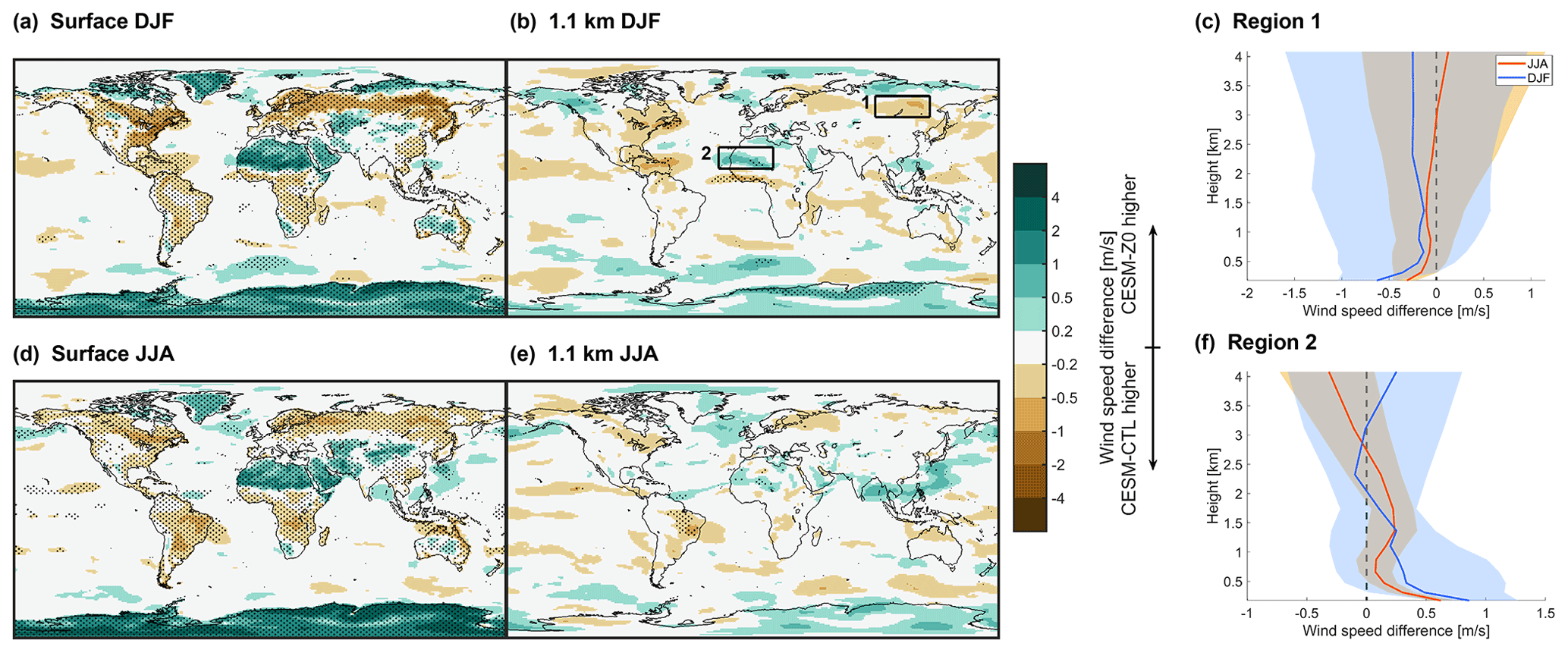
Figure 14 Seasonal mean wind speed difference of CESM-Z0 minus CESM-CTL at lowest atmospheric level (a, d) and approximately 1.1 km above sea level (b, e). Top row shows boreal winter (DJF) and bottom row boreal summer (JJA). The stippling shows areas with a difference that is statistically significant different from 0 in a two-sided t test at the 95 % confidence level with a controlled false discovery rate. Note the non-linear color scale. Panels (c) and (f) show the profile of area-weighted mean wind speed difference in DJF (blue) and JJA (red) in regions 1 (c) and 2 (f), which are marked in panel (b). The line depicts the median wind speed difference across all seasonal means and shading shows the range between the 10th and 90th percentiles. Height is calculated assuming a surface pressure of 1013.2 hPa, a surface air temperature of 288.15 K, and a constant lapse rate of 6.5 K km⁻¹. Data from the last 30 years of the spinup period and data from the analysis period (15 years) were used for this figure.

6 Conclusions

In this study, we have compared the representation of z₀ in CLM to observations and parameterizations that exist in the literature, conducted revisions of CLM when clearly supported by this comparison, and assessed the impact of these revisions on simulated temperatures and wind speed. Specifically, we introduced the parameterization proposed by Raupach (1992) for the z_0,v, where parameter choices were optimized to match the observational data of Hu et al. (2020). The z₀ of forests is increased considerably with this new parameterization, while z₀ for crops is decreased. Further, the revised z₀ of broadleaf deciduous forests exhibits a minimum during the growing season as observed in the field. Based on our literature synthesis, the globally constant values for z_0m,b, z_0m,s, and z_0m,i are reduced from $\mathrm{1.0}\times {\mathrm{10}}^{-\mathrm{2}}$ to $\mathrm{8.4}\times {\mathrm{10}}^{-\mathrm{4}}$ m, from $\mathrm{2.4}\times {\mathrm{10}}^{-\mathrm{3}}$ to $\mathrm{7.8}\times {\mathrm{10}}^{-\mathrm{4}}$ m, and from $\mathrm{1.0}\times {\mathrm{10}}^{-\mathrm{2}}$ to $\mathrm{2.3}\times {\mathrm{10}}^{-\mathrm{3}}$ m, respectively. Alternatively, the spatially explicit z_0m,b input field from Prigent et al. (2005) can be activated in the revised model version. Similarly, the user may activate the parameterization of Brock et al. (2006) for z_0m,s as a function of accumulated snowmelt. Finally, we replace the parameterization of Zeng and Dickinson (1998) for z_0h,g and z_0q,g with the parameterization of Yang et al. (2008). Overall, our proposed modifications increase z_0m in most areas dominated by vegetation, while z_0m is decreased considerably in desert regions.

The decrease of z_0m,g is found to warm the land surface in warm deserts during the day and, to a lesser extent, also at night. The LST decreases over the cold deserts in particular during the winter season. The impact of the raised z_0,v varies diurnally, with a cooling effect during day and a warming effect at night. In land–atmosphere coupled simulations, the daytime warming of LST over warm deserts is amplified compared to land-only simulations due to a decrease in cloud cover leading to an increase in incoming solar radiation. Overall, the proposed model modifications reduce biases in the LST DTR compared to MODIS both over warm deserts, where the DTR is underestimated, and in regions dominated by forests, where the DTR tends to be overestimated. Also, the revisions of z₀ alter the local LST response to a conversion of vegetation to bare land, which could be relevant for the simulated biogeophysical effect of desertification. The sensitivity of the LST at 13:30 and the DTR improves in CLM-Z0, while the nighttime sensitivity deteriorates compared to Du18. The response in the TBOT DTR in CESM opposes the sign of the LST DTR response, with an amplification in forested regions and a dampening over warm deserts. Surface wind speeds increase over desert areas, while they decrease in regions with forests. These alterations in surface wind speed typically disappear beyond approximately 1 km above the land surface.

Overall, our results highlight the importance of z₀ for the exchange of energy, water, and momentum between the land surface and the atmosphere and through that for surface temperatures and wind speed. Beyond these, there are several potential impacts we did not explore in this study. For example, we did not evaluate how these changes might affect the exchange of greenhouse gases between the land and the atmosphere, be it directly through alterations of the turbulent exchange of such gases or indirectly through biogeophysical effects that affect biogeochemical processes such as photosynthesis or respiration. Further, the resultant increase in surface wind speed in arid and semi-arid regions are likely to affect mineral dust emissions and might thereby alter dust aerosol loading in the atmosphere (Csavina et al., 2014; Wu et al., 2019).

Even though our revisions of z₀ oftentimes improve the simulated LST DTR compared to MODIS, some considerable biases persist. Such biases are at least partly related to inadequate properties of the land surface other than z₀. For example, the surface emissivity varies considerably across different types of land cover (Jin and Liang, 2006). Values as low as 0.9 are observed over the Sahara, which is much lower than the prescribed value of 0.96 for soils used in CLM and might therefore affect simulated LSTs compared to MODIS (Jin and Liang, 2006). Next, z_0h,g and z_0q,g frequently exceed z_0m,g in the revised model, since the formulation of Yang et al. (2008) often increases z_0h,g and z_0q,g while z_0m,g is decreased. Field studies on the other hand only rarely observe lower values for z_0m,g than z_0h,g and z_0q,g. This behavior highlights a potential drawback of the formulation of Yang et al. (2008), which decouples z_0h,g and z_0q,g to some extent from z_0m,g. This feature is unique compared to most other formulations in the literature that link z_0h,g and z_0q,g directly to z_0m,g. Nevertheless, the two modifications in combination improved the diurnal LST variability compared to MODIS over most desert areas. For vegetation, several development activities are underway within CLM to improve the diurnal variability of temperatures and surface fluxes. Bonan et al. (2018) replace the big-leaf approach in CLM with a multi-layer canopy and introduce a roughness sublayer parameterization for tall canopies. The latter modification could ultimately replace z_0,v entirely. Further, the recent addition of biomass heat storage to CLM improved the realism of simulated energy fluxes and LSTs over forests (Swenson et al., 2019; Meier et al., 2019). Finally, some discrepancies between our simulations and MODIS could also be related to the atmospheric forcing fields that CLM receives, be it from the GSWP3 reanalysis data in the case of the land-only simulations or from the atmospheric component of CESM for the coupled simulations.

While observations of z₀ provide valuable information for model development, the assumptions within the model world can differ from the assumptions made to estimate z₀ in the field. For example, the formulations for the stability correction functions in Hu20 differ from the ones used in CLM. Consequently, CLM would produce slightly different turbulent fluxes than measured in the field, even if conditions are exactly the same. We would like to highlight that the current approach in CLM of dividing grid cells into tiles of differing land covers does not specify how the different land covers are situated within this cell. For example, CLM treats a savanna covered by sparse trees and grasses the same as one large forest next to a grassland landscape (given that the two types of vegetation and the area fraction covered by each vegetation type are roughly the same). But in terms of z₀ and other surface properties these two landscapes differ. It might therefore be necessary to further refine the tile approach in CLM, such that these two landscapes may be distinguished. In CLM, the ecosystem demography model FATES resolves this issue to some extent (Fisher et al., 2015). However, our updates of z_0,v after Ra92 are not yet implemented in this version of the model.

We would like to emphasize the value of z₀ observations for this work but also for other efforts of model and parameterization development. Several decades of observations of z₀ allow for better constraint of models and a better understanding of how z₀ is influenced by conditions at the land surface. Yet, knowledge gaps remain, for example for ice sheets. In situ observations indicate that z_0m,i varies substantially, likely related to variations in the structure of the ice (Brock et al., 2006; Fitzpatrick et al., 2019). However, the surface structure of the ice is not explicitly simulated in Earth system models. Remote-sensing-based data of z_0m,i over the ice sheets might be a good solution to capture such spatial variations in z_0m,i, similar to what already exists for z_0m,b (e.g., Prigent et al., 2005). In urban environments, z₀ is not only closely linked to mean building height and the density of buildings but also to the variability of the building height (Nakayama et al., 2011; Kanda et al., 2013). If a global data set of variability of building heights becomes available, it could therefore be considered as an additional input variable to compute z₀ in the urban module of CLM. For vegetation, we focused on the z₀ for the exchange between the canopy air space and the free atmosphere, but did not consider the conductances for sensible and latent heat between the leaves/ground and the canopy air space. Hu et al. (2020) and the recent study of Young et al. (2021) focus both on z_0h,v alongside z_0m,v. Future studies could therefore develop a framework to confront the leaf surface conductance for sensible heat in CLM with such observational constraints of z_0h,v.

Appendix A

A1 Sensitivity tests to isolate contributions from individual modifications

Besides CLM-CTL and CLM-Z0, we run a number of additional 15-year simulations, which are summarized in Table A1, to better understand the importance of the individual modifications introduced in CLM-Z0. First of all, we run a simulation, CLM-Z0C, that follows the same protocol as CLM-Z0 but with the median values for z_0m,b and z_0m,s depicted in Fig. 2 instead of using the spatially explicit data of Prigent et al. (2005) and the parameterization of Brock et al. (2006), respectively. This simulation uses the initial conditions from the spinup of CLM-Z0. Additionally, we start three simulations starting from the initial conditions of CLM-CTL that only utilize a subset of the modifications described in the Sect. 2. CLM-VEG uses only the parameterization of Raupach (1992) for z_0,v but preserves the default for z₀ otherwise. In CLM-Z0M, we introduce all the modifications related to z_0m but retain the formulation of Zeng and Dickinson (1998) for z_0h,g and z_0q,g. CLM-Ya08 on the other hand applies the formulation of Yang et al. (2008) for z_0h,g and z_0q,g and uses the default representation of z_0m. For this analysis, we use the years 1998–2002 as an additional spinup period and only analyze 2003–2012.

Zeng and Wang (2007)Zeng and Dickinson (1998)Raupach (1992)Prigent et al. (2005)Brock et al. (2006)Yang et al. (2008)Raupach (1992)Yang et al. (2008)Raupach (1992)Zeng and Dickinson (1998)Raupach (1992)Prigent et al. (2005)Brock et al. (2006)Zeng and Dickinson (1998)Zeng and Wang (2007)Yang et al. (2008)

Table A1 Overview of CLM simulations. Columns from left to right show the name of simulation, parameterization for z_0,v, z_0m,b z_0m,s, choice of z_0m,i, parameterization for z_0h,g and z_0q,g, and initial conditions used. Parameterizations and data sets that are marked with a asterisk were modified before including them in CLM.

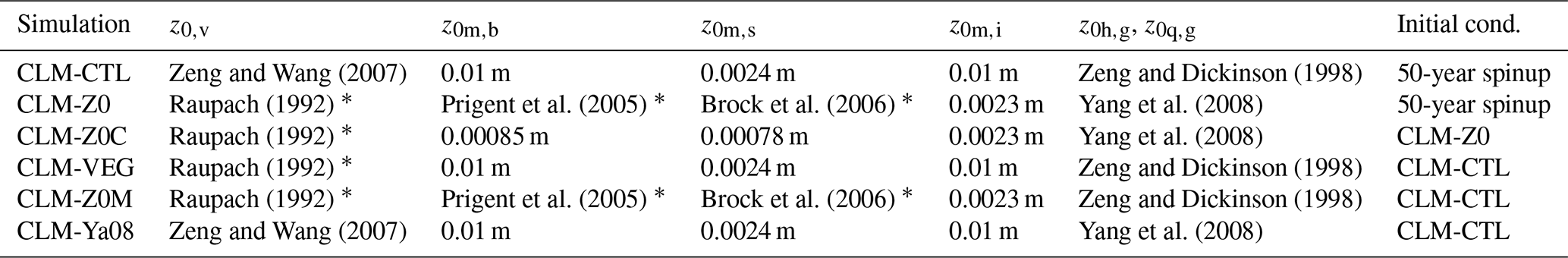
Figure A1 Difference in LST DTR over 2003–2012 for (a) CLM-Z0 minus CLM-CTL, (b) CLM-VEG minus CLM-CTL, (c) CLM-Z0M minus CLM-CTL, (d) CLM-Ya08 minus CLM-CTL, (e) CLM-Z0C minus CLM-CTL, and (f) CLM-Z0 minus CLM-Z0M.

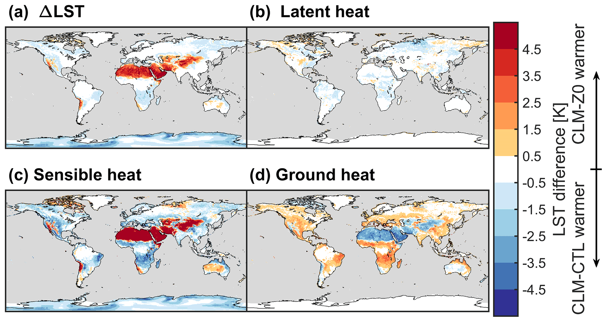
Figure A2 Energy balance decomposition for change in LST at 13:30 local solar time in boreal summer of CLM-Z0 minus CLM-CTL. (a) Change in LST, (b) contribution from change in latent heat, (c) contribution from change in sensible heat, and (d) contribution from change in ground heat flux. Note that some terms are not shown because they are zero in offline simulations (incoming radiation terms) or because they are small (albedo and the imbalance term).

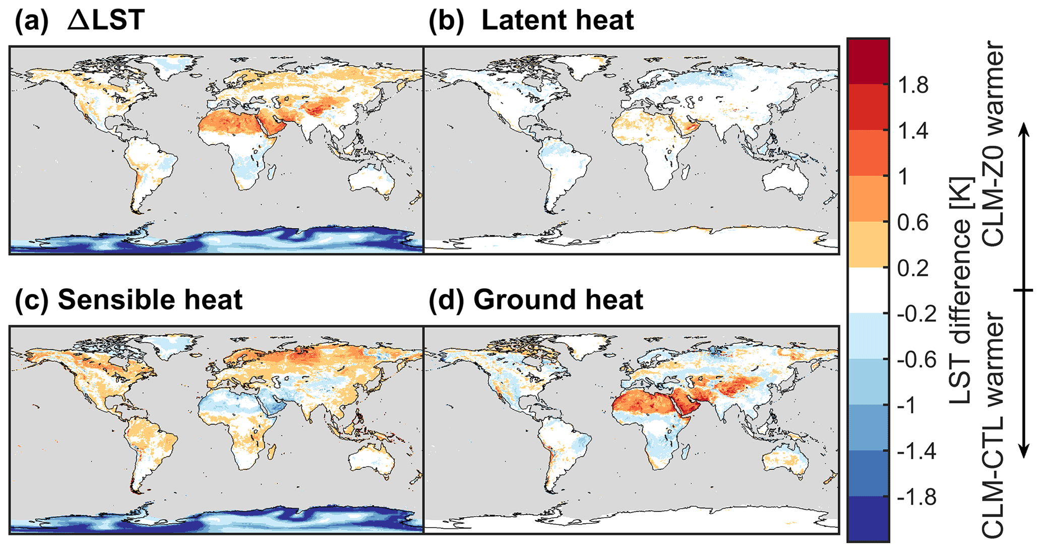
Figure A3 As Fig. A2 but at 01:30 local solar time.

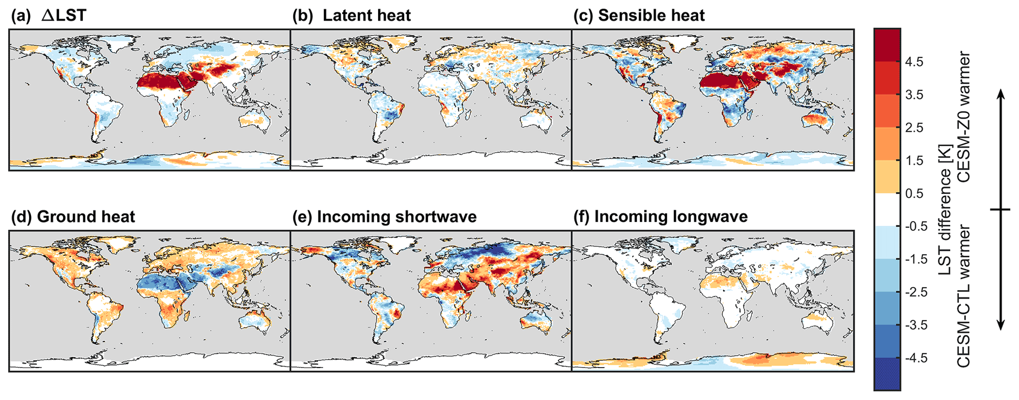
Figure A4 Energy balance decomposition for change in LST at 13:30 local solar time in boreal summer of CESM-Z0 minus CESM-CTL. (a) Change in LST, (b) contribution from change in latent heat, (c) contribution from change in sensible heat, (d) contribution from change in ground heat flux, (e) contribution from change in incoming shortwave radiation, and (f) contribution from change in incoming longwave radiation. Note that the albedo and the imbalance term are not shown because they are small.

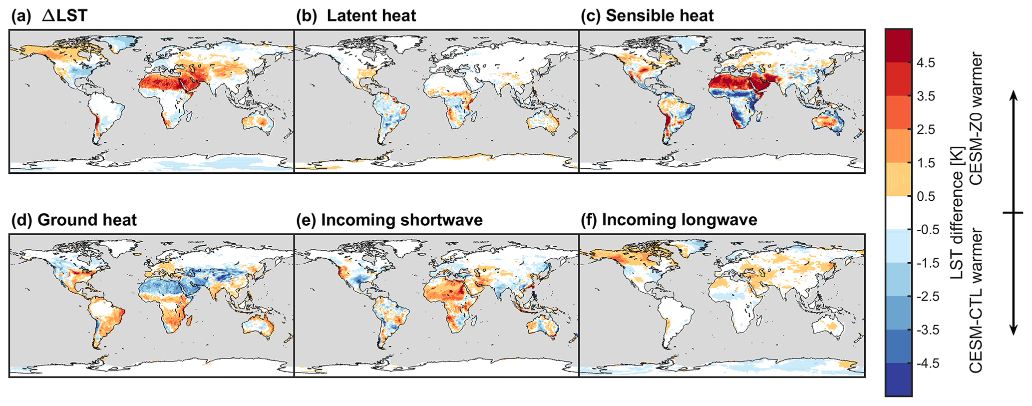
Figure A5 As Fig. A4 but for boreal winter.

Figure A6 As Fig. 12a and b but using data of the analysis period only (a, b, December 1998 to November 2012) and using data from the last 30 years of the spinup period (c, d, December 1968 to November 1998).

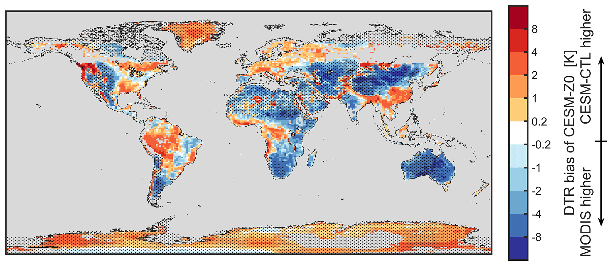
Figure A7 As Fig. 11d but for CESM-Z0.

Duveiller et al. (2018)Hu et al. (2020)Prigent et al. (2005)Berger (1978)Raupach (1992)Raupach (1994)Yang et al. (2008)

Table A2 List of abbreviations and symbols used in this study. Symbols that only appear in one equation are not listed.

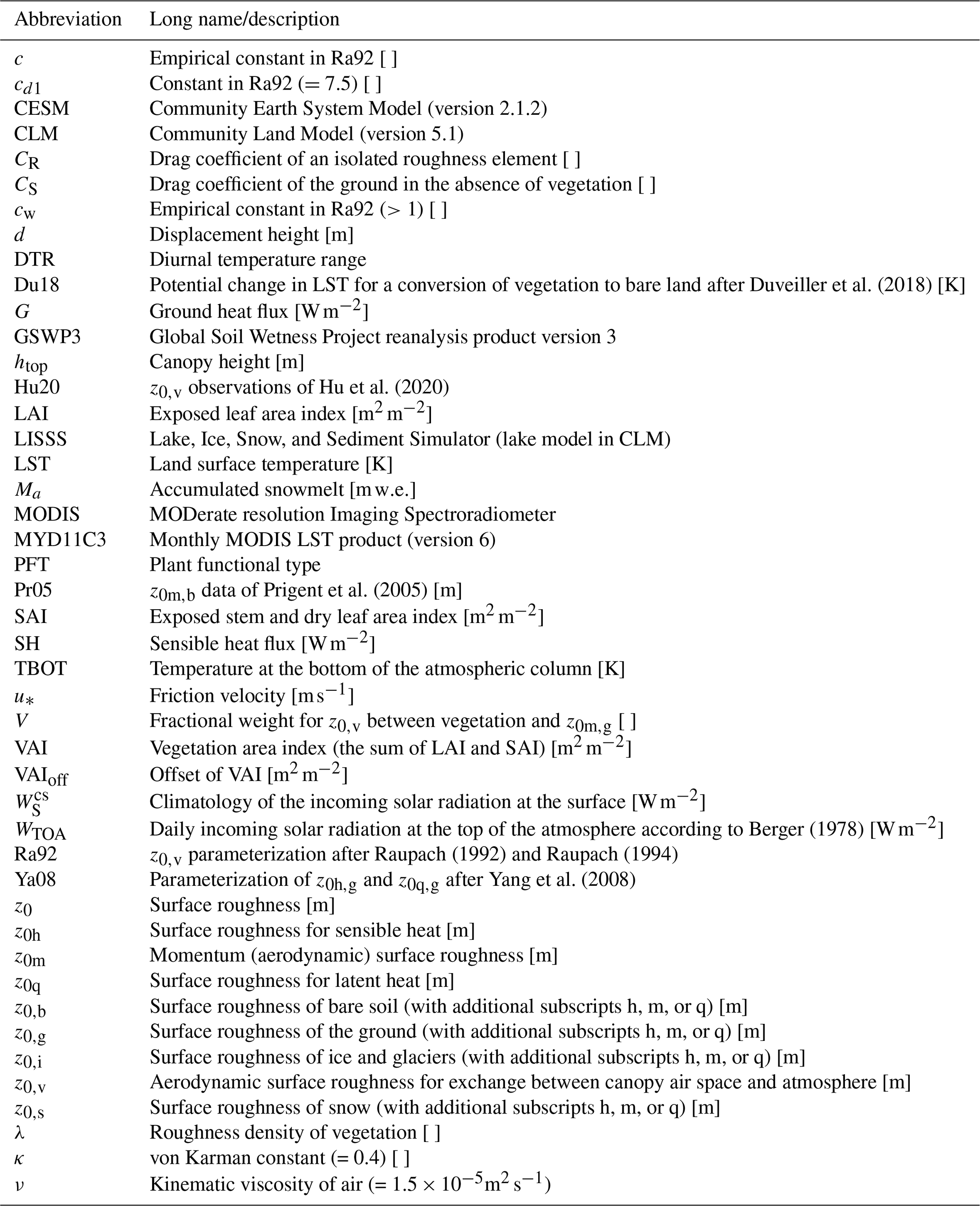
Here, we compare the effect on the annual mean LST DTR of the different sensitivity experiments in comparison to CLM-CTL. The alterations in z_0,v alone introduced in CLM-VEG decrease the DTR in regions dominated by forests (where the z_0,v is increased) and increase it in regions with a considerable amount of crops (for which z_0,v is decreased; Fig. A1b). Interestingly, the response in forested regions is often weaker in CLM-VEG than in CLM-Z0 or even reversed in sign in central North America (Fig. A1a). The full signal strength in regions dominated by vegetation only emerges, when the alterations of z_0m,g are introduced in CLM-Z0M (Fig. A1c). It appears that a decrease in z_0m,g under a closed canopy dampens the LST DTR more than an increase in z_0,v in isolation. The opposite is the case over warm desert areas. Somewhat unexpected, the amplifications of diurnal variations in LST over arid and semi-arid regions is moderated when Ya08 is introduced in CLM-Z0 compared CLM-Z0M over most of the Sahara, the Middle East, and the Himalaya (Fig. A1f). On the other hand, the introduction of the Ya08 parameterization for z_0h,g and z_0q,g with the default z_0m,g in CLM-Ya08 enhances the LST DTR (Fig. A1d). Ya08 therefore amplifies the diurnal LST variability for relatively large values of z_0m,g (which are used in CLM-Ya08 and CLM-CTL), while it dampens this variability for small z_0m,g values (which are used in CLM-Z0M and CLM-Z0) compared to the parameterization of Zeng and Dickinson (1998). The globally constant z_0m,b in CLM-Z0C is larger than the spatially explicit data in Pr05 (Fig. 2). Also, z_0m,s is higher in CLM-Z0C over most regions than in CLM-Z0, with the notable exception of some areas of Greenland (not shown). Thus, z_0m,g is generally decreased less in CLM-Z0C than in CLM-Z0 in comparison to CLM-CTL. Accordingly, the response in the LST DTR tends to be slightly smaller in magnitude in CLM-Z0C than in CLM-Z0 (Fig. A1a and e). Overall, there is however no major difference between CLM-Z0C and CLM-Z0.

A2 Energy balance decomposition

In this section, we present an energy balance decomposition after Luyssaert et al. (2014) to better understand the contribution of changes in individual energy fluxes to the overall change in LST between CLM/CESM-CTL and CLM/CESM-Z0. Assuming the emissivity of the land surface is equal to 1, the change in LST (ΔLST) is expressed as follows:

$$\begin{array}{}\text{(A1)}& \begin{array}{rl}\mathrm{\Delta }\text{LST}& ={\displaystyle \frac{\mathrm{1}}{\mathrm{4}\mathit{\sigma }{\text{LST}}^{\mathrm{3}}}}\left(-{\text{SW}}_{\mathrm{in}}\mathrm{\Delta }\mathit{\alpha }+(\mathrm{1}-\mathit{\alpha })\mathrm{\Delta }{\text{SW}}_{\mathrm{in}}\right.\\ & \left.+\mathrm{\Delta }{\text{LW}}_{\mathrm{in}}-\mathrm{\Delta }\text{LH}-\mathrm{\Delta }\text{SH}-\mathrm{\Delta }G-\mathrm{\Delta }I\right),\end{array}\end{array}$$

where σ is the Stefan–Boltzmann constant, SW_in is the incoming shortwave radiation, α is the albedo, LW_in is the incoming longwave radiation, LH is the latent heat flux, SH is the sensible heat flux, G is the ground heat flux, and I is the energy imbalance. ΔX corresponds to the difference in variable X between CLM/CESM-Z0 and CLM/CESM-CTL. We take the average of CLM/CESM-Z0 and CLM/CESM-CTL for the variables for which no difference is taken (e.g., SW_in for the first term in the brackets). The terms on the right-hand side of Eq. (A1) correspond to the change in LST due to the change in albedo, incoming shortwave radiation, incoming longwave radiation, latent heat, sensible heat, ground heat, and the energy imbalance from left to right.

Figure A2 shows the most important terms of the energy balance decomposition at 13:30 local solar time during boreal summer in the offline simulations. Changes in LST during the day between CLM-CTL and CLM-Z0 are mostly the result of alterations in SH. The contribution from SH is compensated partly by G most of the time. If, for example, the LST increases due to a reduction in SH, part of this energy surplus is compensated by the energy stored in the ground (leading to a warming of the soils below the land surface). The other terms only have a small effect on the overall change in LST. At 01:30 local solar time, ΔLST is again driven by changes in SH in the high latitudes (Fig. A2). At lower latitudes, in particular in the warm deserts, the strong LST response during the day frequently translates into the night through the energy stored in the ground. Over the Sahara, for example, the ground absorbs more energy during the day because SH is reduced, resulting in a warmer LST at night.

For the land–atmosphere coupled simulations, the incoming shortwave and longwave radiation terms become relevant due to atmospheric feedbacks. During boreal summer, increased incoming solar radiation over the Sahara, the Middle East, and the Himalaya amplify the warming from the reduced SH (Fig. A4). The reduction in LST over the northern midlatitudes and high latitudes mostly coincides with less incoming solar radiation. In contrast, the signal in winter is determined by the longwave radiation in those regions (Fig. A5). In particular, the wintertime warming of the LST in the northern part of North America occurs due to more incoming longwave radiation in concert with warmer atmospheric temperatures (Fig. A6a).