the Creative Commons Attribution 4.0 License.
the Creative Commons Attribution 4.0 License.
 | 15 Mar 2022
DINCAE 2.0: multivariate convolutional neural network with error estimates to reconstruct sea surface temperature satellite and altimetry observations
Aida Alvera-Azcárate
Charles Troupin
Jean-Marie Beckers
DINCAE (Data INterpolating Convolutional Auto-Encoder) is a neural network used to reconstruct missing data (e.g., obscured by clouds or gaps between tracks) in satellite data. Contrary to standard image reconstruction (in-painting) with neural networks, this application requires a method to handle missing data (or data with variable accuracy) already in the training phase. Instead of using a standard L2 (or L1) cost function, the neural network (U-Net type of network) is optimized by minimizing the negative log likelihood assuming a Gaussian distribution (characterized by a mean and a variance). As a consequence, the neural network also provides an expected error variance of the reconstructed field (per pixel and per time instance).
In this updated version DINCAE 2.0, the code was rewritten in Julia and a new type of skip connection has been implemented which showed superior performance with respect to the previous version. The method has also been extended to handle multivariate data (an example will be shown with sea surface temperature, chlorophyll concentration and wind fields). The improvement of this network is demonstrated for the Adriatic Sea.
Convolutional networks work usually with gridded data as input. This is however a limitation for some data types used in oceanography and in Earth sciences in general, where observations are often irregularly sampled. The first layer of the neural network and the cost function have been modified so that unstructured data can also be used as inputs to obtain gridded fields as output. To demonstrate this, the neural network is applied to along-track altimetry data in the Mediterranean Sea. Results from a 20-year reconstruction are presented and validated. Hyperparameters are determined using Bayesian optimization and minimizing the error relative to a development dataset.
- Article
(5225 KB) - Full-text XML
- BibTeX
- EndNote


Ocean data are generally sparse and inhomogeneously distributed. The data coverage often contains large gaps in space and time. This is in particular the case with in situ observations. Satellite remote sensing only measures the surface of the ocean but generally has better spatial coverage than in situ observations. However, still about 75 % of the ocean surface is on average covered by clouds that block sensors in the optical and infrared bands (Wylie et al., 2005). Given the sparsity of data, it is natural to aim to combine data representing different parameters as, e.g., mesoscale flow structures are often visible in all ocean tracers.
Prior work on using multivariate data in connection with satellite data use, for example, empirical orthogonal functions (EOF), which can be naturally extended to multivariate datasets as long as an appropriate norm is defined. For example, Alvera-Azcárate et al. (2007) uses sea surface temperature, chlorophyll and wind satellite fields with data interpolating empirical orthogonal functions (DINEOF). Multivariate EOFs have also been used to project surface observations to deeper layers (Nardelli and Santoleri, 2005) or to derive nitrate maps in the Southern Ocean (Liang et al., 2018). In the latter case, EOFs linking salinity, and potential temperature and nitrate concentrations are derived from model simulations.
As some observations can be measured at much high spatial resolution via remote sensing (in particular the resolution of sea surface temperature is much higher than the resolution of sea surface salinity products), “multifractal fusion techniques” are used to improve remote sensed surface salinity estimates using sea surface temperature. Data fusion is implemented as a locally weighted linear regression (Olmedo et al., 2018, 2021). Han et al. (2020) also used an earlier version of the DINCAE code to estimate sea surface chlorophyll using additional sea surface temperature observations.
The structure of a neural network, and in particular its depth, is uncertain and to some degree dependent on the used data set. We also investigate the influence of the depth of the neural networks in this work. It is known that neural networks are increasingly more difficult to train as their depth increases because of the well-known vanishing gradient problem (Hochreiter, 1998): the derivative of the loss function relative to the weights of the first layers of a neural network has the tendency to either decrease (or increase) exponentially with a increasing number of layers. This prevents effective optimization (training) of these layers using gradient-based optimization methods.
Several methods have been proposed in the literature to mitigate such problems using alternative neural network architectures. In the context of the present manuscript, skip connections in the form of residual layers have been tested (similar to residual networks; He et al., 2016). The derivative of the loss function relative to the weights in such layers remains (at least initially) closer to one, so there is a more direct relationship between the loss function and the weights and biases to be optimized. Deeper residual networks include shallower networks as a special case and thus, as per their construction, should perform at least as well as shallower networks.
The gradient of a whole network is computed via back-propagation, which is essentially based on the repeated application of the chain rule for differentiation. The information of the observation is injected via the loss function and propagated backward in a way which is similar to the 4D-var backward in time integration of the adjoint model. Another interesting neural network architecture has been proposed in the form of the Inception network (Szegedy et al., 2015), where the output of intermediate layers, here in the form of a preliminary reconstruction, are used in the loss function (in addition to the output of the final layer). The result is that the information of the observations are injected not only at the final layer but also in the intermediate layer, which also contributes to reducing the vanishing gradient problem.
While for gridded satellite data, approaches based on empirical orthogonal functions and convolutional neural networks have been shown the be successful, it is difficult to apply similar concepts to non-gridded data as these methods typically require a stationary grid. Another objective of this paper is to show how convolutional neural networks can be used on non-gridded data. This approach is illustrated with altimetry observations.
The objective of this manuscript is to highlight the improvement of DINCAE relative to the previously published version (Barth et al., 2020). The Sect. 2 presents the updated structure of the neural network. The gridded and non-gridded observations used here are presented in Sect. 3. Details of the implementation are also given (Sect. 4). The results and conclusions are presented in Sects. 5 and 6.
The DINCAE network (Barth et al., 2020) is a neural network composed of an encoder and decoder network. The encoder uses the original gappy satellite data (with additional metadata as explained later) and the decoder uses the output of the encoder to reconstruct the full data image (along with an error estimate). The encoder uses a series of convolutional layers followed by max pooling layers, reducing the resolution of the datasets. The decoder does essentially the reverse operation by using convolutional and interpolation layers. This is the general structure of a convolutional autoencoder and the classical U-Net networks (Ronneberger et al., 2015). In the following section we will discuss the main components of the DINCAE neural network used for the different test cases and emphasize the changes relative to the previous version.
2.1 Skip connections
In an autoencoder, the inputs are compressed by forcing the data flow through a bottleneck, which ensures that the neural network must efficiently compress and decompress the information. However, in U-Net (Ronneberger et al., 2015) and DINCAE, skip connections are implemented, allowing the information flow of the network to partially bypass the bottleneck to prevent the loss of small-scale details in the reconstruction. Skip connections can be realized either by concatenating tensors along the feature map dimension (as it is done in U-Net) or by summing the tensors. The cat skip connections at the step l in the autoencoder can be written as the following operation:
where cat concatenates two 3D arrays along the dimension representing the features channels. The function f(l) is a sequence of neural network layers applied to the array of X(l) (produced by previous network layers). Sum skip connections are implemented as
Clearly, the output of a cat skip connection has a size twice as large as the output of a sum skip connection. These skip connections are followed by a convolutional layer, which ensures that the number of output features are the same for both types of skip connection. In fact, one can show that the sum skip connection (followed by a convolution layer) is formally a special case of the cat skip connection. However, sum skip connections can be advantageous because the weight and bias of the convolutional layers are more directly related to the output of the neural network, which helps to reduce the “vanishing gradient problem” (He et al., 2016).
2.2 Refinement step
The whole neural network can be described as two functions that provide the input variable product between the reconstruction and its expected error variance for every grid cell. The loss function is derived from the negative log-likelihood of a Gaussian with mean and variance :
where the sum with the spatial indices i and j runs over all grid points with valid (i.e., non-masked) values and N is the number of valid values. The first term of the right-hand side of the equation is the mean square error, but scaled by the estimated error standard deviation, the second term penalizes any overestimation of the error standard deviation and the third term is constant and can be neglected as it does not influence the gradient of the cost function. For a convolutional auto-encoder with refinement, the intermediate outputs and are concatenated with the inputs and passed through another auto-encoder with the same structure (except for the number of filters for the input layer, which has to accommodate the two additional fields corresponding to and ). The weights of the first and second auto-encoder are not related. The final cost function with refinement Jr is given by
where and are the reconstruction and its expected error variance produced by the second auto-encoder. The weights α and α′ control how much importance is given to the intermediate output (relative to the final output).
With a refinement step, the neural network becomes essentially twice as deep and the number of parameters (approximately) doubles. The increased depth would make it prone to the vanishing gradient problem. However, by including the intermediate results in the cost function, this problem is reduced. In fact, information from the observations is injected during back-propagation by the loss function. Due to the refinement step and the loss function, which also depends on the intermediate result, the information from the observation is injected at the last layer and at the middle layer of the combined neural network (Szegedy et al., 2015). The relationship between the first layers of the neural network and the cost function is therefore more direct, which helps in the training of these first layers.
The refinement step has been used in image in-painting for a computer vision application (Liu et al., 2019) and it has also been applied for oceanographic data for tide gauge data (Zhang et al., 2020). In the present work, only one refinement step is tested, but the code supports an arbitrary number of sequential refinement steps.
2.3 Multivariate reconstructions
Auxiliary satellite data (with potentially missing data) can be provided for the reconstruction. The handling of missing data in these auxiliary data is identical to the way missing data are treated for the primary variable. For every auxiliary satellite data, the average over time is first removed. The auxiliary data (divided by its corresponding error variance) and the inverse of the error variance are provided as input. Where data are missing, the corresponding input values are set to zero representing an infinitely large error (as a consequence of the chosen scaling). Multiple time instances centered around a target time can be provided as input.
2.4 Non-gridded input data
Current satellite altimetry mission measures sea surface height along the ground track of the satellite. Satellite altimetry can measure through clouds but the data are only available along a collection of tracks. In order to better handle such data sets, we extended DINCAE to handle unstructured data as input.
The first layer in DINCAE is a convolutional layer, which typically requires a field discretized on a rectangular grid. The convolutional layer can be seen as the discretized version of the following integral:
where f is the input field, w are the weights in the convolution (also called convolution kernel), Ωw is the support of the function w (i.e., the domain where w is different from zero) and g the output of the convolutional layer. To discretize the integral, the continuous function f is replaced by a sum of Dirac functions using the values fi,j defined on a regular grid:
In this case, the continuous convolution becomes the standard discrete convolution as used in neural networks. The weights w(x,y) only need to be known at the discrete locations defined by the underlying grid.
For data points which are not defined on a regular grid we essentially use a similar approach. The function f is again written as a sum of Dirac functions:
where now fk are the values at the locations (xk,yk), which can be arbitrary. In order to evaluate the integral (Eq. 5), it is necessary to know the weights at the location (xk,yk). The weights are still discretized on a regular grid, but are interpolated bilinearly to the data location to evaluate the integral. In fact, instead of interpolating the weights w, one can also apply the adjoint of the linear interpolation to fk (which is mathematically equivalent). This has the benefit that the computation of the convolution can be implemented using the optimized functions in the neural network library.
For data defined on a regular grid, it has been verified numerically that this proposed approach and the traditional approach used to compute the convolution give the same results.
The improvements are examined in two test cases. For multivariate gridded data, the approach is tested with sea surface temperature, chlorophyll and winds on the Adriatic Sea; for non-gridded data altimetry, observations of the whole Mediterranean Sea were used. As the altimetry observations do not resolve as many small scales as sea surface temperature, a larger domain was chosen for the altimetry test case.
3.1 Gridded data (Adriatic Sea)
As the previous application (Barth et al., 2020) considered relatively low-resolution AVHRR data, we used more modern and higher-resolution satellite data in this application for the Adriatic Sea. The datasets used include the following.
-
Sea Surface Temperature (MODIS Terra Level 3 SST Thermal IR Daily 4km Nighttime v2014.0, https://doi.org/10.5067/MODST-1D4N4, OBPG, 2015) made available by PO.DAAC (https://podaac.jpl.nasa.gov/, last access: 10 February 2022, JPL, NASA, USA).
-
Wind speed (Cross-Calibrated Multi-Platform, CCMP; gridded surface vector winds) made available from Remote Sensing Systems (http://www.remss.com/measurements/ccmp/, last access: 19 July 2019, Wentz et al., 2019). These datasets are described in Atlas et al. (2011), Mears et al. (2019) and Wentz et al. (2019). This dataset has a 6 h temporal resolution and a ∘ spatial resolution . The wind fields are averaged as daily mean fields.
-
Chlorophyll a from Ocean Biology Processing Group, NASA Goddard Space Flight Center et al. (2018), https://oceancolor.gsfc.nasa.gov/data/overview/ (last access: 18 September 2019) at a 4 km resolution and L3 processing level.
The data sets span the time period 1 January 2003 to 31 December 2016. They are all interpolated (using bi-linear interpolation) on the common grid defined by the SST fields.
As ocean mixing reacts to the averaged effect of the wind speed (norm of the wind vector), we also smoothed the speed with a Laplacian filter using a time period of 2.2 d and a lag of 4 d (wind speed preceding SST). The optimal lag and time period were obtained by maximizing the correlation between the smoothed wind field and SST from the training data.
3.2 Non-gridded data (Mediterranean Sea)
Altimetry data from 1 January 1993 to 13 May 2019 covering 7∘ W to 37∘ E and from 30 to 46∘ N from 22 satellite missions operating during this time frame are used. This domain essentially contains the Mediterranean Sea but also a small part of the Bay of Biscay and the Black Sea. In preliminary studies we found that including the data from adjacent seas can help neural networks better generalize and prevent overfitting (e.g., Gong et al., 2019) as the neural network is confronted with a more diverse set of conditions. The data (SEALEVEL_EUR_PHY_L3_MY_OBSERVATIONS_008_061, accessed on 13 October 2020) are made available by the Copernicus Marine Environment Monitoring Service (CMEMS).
These data were split along the following fractions:
-
70 % training data,
-
20 % development data,
-
10 % test data.
To reduce the correlation between the different datasets, satellite tracks are not split and belong entirely to one of these three datasets.
Some experiments of the reconstructed altimetry use gridded sea surface temperature satellite observations as an auxiliary dataset for multivariate reconstruction. We use the AVHRR_OI-NCEI-L4-GLOB-v2.0 datasets (Reynolds et al., 2007; National Centers for Environmental Information, 2016) because it is a single consistent dataset covering the full time period of the altimetry data and because it matches approximately the altimetry dataset in terms of resolved spatial scales.
Python code was first ported from TensorFlow 1.12 to 1.15, reducing the training time from 4.5 to 3.5 h using a GeForce GTX 1080 GPU and Intel Core i7-7700 CPU. We also considered porting DINCAE to TensorFlow 2. The TensorFlow 2 programming interface is however quite different from previous versions. As our group gained familiarity with the Julia programming language (Bezanson et al., 2017), we decided to rewrite DINCAE in Julia. Porting DINCAE to Julia with the package Knet (Yuret, 2016) cut down the runtime from 3.5 to 1.9 h (thanks to more efficient data transformation) using the AVHRR dataset described in Barth et al. (2020), and using a concatenation skip connection in both cases.
For the Adriatic test case, the input is a 3D array with the dimension corresponding to the longitude, latitude and the different parameters. The input parameters for an univariate reconstruction are three time instances of temperature scaled by the inverse of the error variance (previous, current and next day), the corresponding inverse of the error variance, the longitude and latitude of every grid cell and the sine and cosine of the day of the year multiplied by as in Barth et al. (2020). The assembled array has a size of elements (for a single training sample). The input is processed by the encoder which is composed of five convolutional layers (with 16, 30, 58, 110 and 209 output filters) with a kernel size of 3×3 and a rectified linear unit (RELU) activation function followed by a max pooling layer with a size of 2×2. The RELU activation function is commonly used in neural networks and is defined by .
The output of the encoder is transformed back to a full image by the decoder, which mirrors the structure of the encoder. The decoder is composed of five upsampling layers (nearest-neighborhood interpolation or bilinear interpolation) followed by a convolutional layer with the equivalent number output filters from the encoder (except for the final layer, which has only two outputs related to the reconstruction and its error variance). The final layer produces a 3D-array (size ) from which the reconstruction and its error variance are computed by
where the parameters γ and μ are set to 10 and 10−3, respectively. The minimum and maximum functions (min and max) are introduced here to prevent division by a value close to zero or the exponentiation of a too-large value. This stabilizes the neural network during the initial phase of the training as the weights and biases are randomly initialized.
In Barth et al. (2020), after the convolutional layers, the model included two fully connected layers (with drop-out). This is no longer used as such layers require that the input matrix for training has exactly the same size as the input matrix of the reconstruction (inference), which makes this architecture difficult for large input arrays (which would arise for global or basin-wide sea surface temperature fields for example). The benefit of replacing dense layers by convolutional layers is further discussed in Long et al. (2015).
Table 1Layers of the neural network for the gridded datasets. Note that every convolution is followed by a RELU activation function.
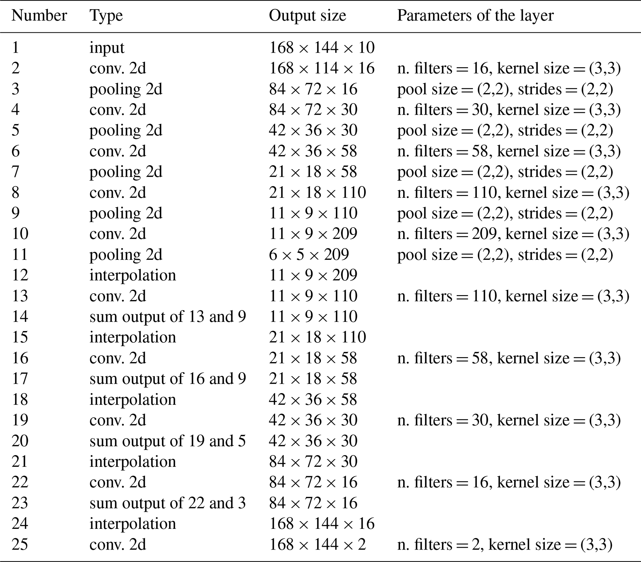
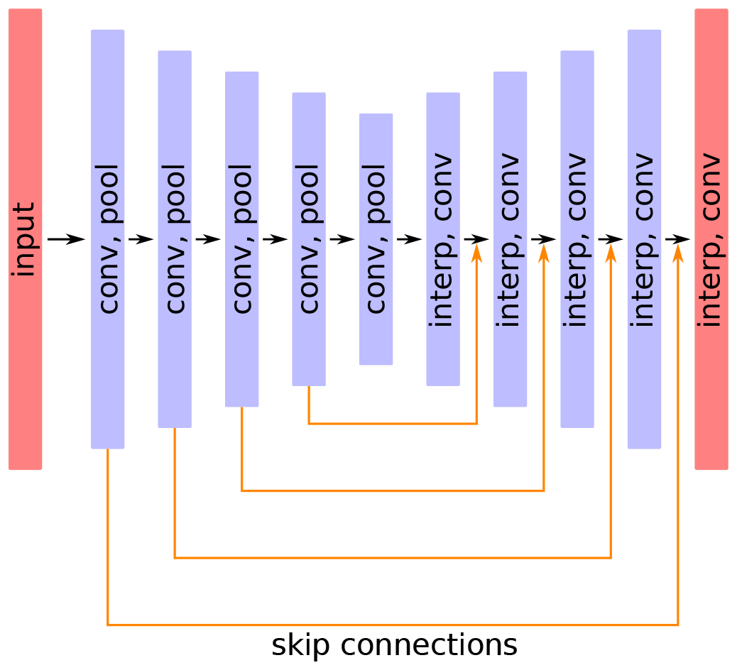
Figure 1General structure of the DINCAE with 2D convolution (conv), max pooling (pool) and interpolation layers (interp). All 2D convolutions are followed by a RELU activation function.

Figure 2DINCAE with a refinement step composed essentially by two sequential autoencoders coupled such that the second autoencoder uses the output of the first and the input data.
The altimetry data were analyzed on a 0.25∘ resolution grid covering the area from 7∘ W and 37∘ E and 30 to 46∘ N. For this neural network implementation, the input size is 177 × 69. The resolution is progressively reduced to 89 × 35, 45 × 18 and 23 × 9 by convolutional layers followed by max pooling layers with 32, 64 and 96 convolutional filters, respectively. Skip connections are implemented after the second convolutional layer onwards.
During training, Gaussian noise with a standard deviation σpos is added to the position of the measurements and every track of the current date has a certain probability pdrop to be withheld from the input of the neural network. The loss function is computed only on tracks from the current date. This helps the neural network to learn how to spread the information spatially. The neural network is optimized during 1000 epochs and the intermediate results are saved every 25 epochs.
The altimetry test case illustrates the results for a non-gridded dataset. Sea surface altimetry is usually gridded with a method like optimal interpolation or variational analysis. The latter can also be seen as a special case of optimal interpolation. For the autoencoder, the following fields are used as inputs:
-
longitude and latitude of the measurement;
-
day of the year (sine and cosine) of the measurement multiplied by where Ty is 365.25 (the length of a year in days);
-
all data within a given centered time window of length Δtwin. For instance if the time window of length Δtwin is 9, the data from the current day are used as well as the tracks from the 4 previous days and the 4 following days.
As in Barth et al. (2020), instead of using the observations directly, the observations are divided by their respective error variance and the inverse of the error variance is used as input. Due to this scaling, it follows that missing data results in a zero input value as it corresponds to a data point with an “infinitely” large error.
The training is done using mini-batches of size nbatch. The weights and biases in the neural network are updated using the gradient of the loss function evaluated at a batch of nbatch time instances (chosen at random). Evaluating the gradient using a subset of the training data chosen at random introduces some stochastic fluctuation allowing the optimization procedure to escape a local minima.
All numerical experiments used the Adam optimizer (Kingma and Ba, 2014) with the standard parameter for the exponential decay rate for the first moment β1=0.9, and for the second moment β1=0.999, and a regularization parameter . The learning rate αn is computed for every n-th epoch as follows:
where α0 is the initial learning rate and γdecay controls the exponential decay of the learning rate: every epochs, the learning rates is halved. If γdecay is zero, then the learning rate is kept constant.
The batch size includes 32 time instances (all hyper-parameters are determined via Bayesian optimization as described further on). The learning rate for the Adam optimizer is 0.00058. The L2 regularization on the weights has been set to a β value of 10−4. The upsampling method can either be nearest neighbor or bilinear interpolation. In our tests, nearest neighbor provided the lowest RMS error relative to the development dataset. The absolute value of the gradients is clipped to 5 in order to stabilize the training. Satellite tracks from Δtwin=27 time days (centered around the target time) are used to derive gridded altimetry data.
The hyper-parameters of the neural network mentioned previously have been determined by Bayesian optimization (Mockus et al., 1978; Jones et al., 1998; Snoek et al., 2012) by minimizing the RMS error relative to the development dataset. The “expected improvement acquisition function” (Mockus et al., 1978) is used to determine which sequence of parameter values is to be evaluated. Bayesian optimization as implemented by the Python package scikit-optimize (Head et al., 2020) was used in these tests.
5.1 Gridded data
The new type of skip connection was first tested with the AVHRR Test case from the Ligurian Sea (Barth et al., 2020). The previous best result (in terms of RMS) was 0.3835 ∘C using the cat skip connection. With the new approach this RMS error is reduced to 0.3604 ∘C. The new type of skip connection makes the neural network more similar to residual networks, which have been shown to be highly successful for image recognition tasks and allow for training deep networks more easily (He et al., 2016).
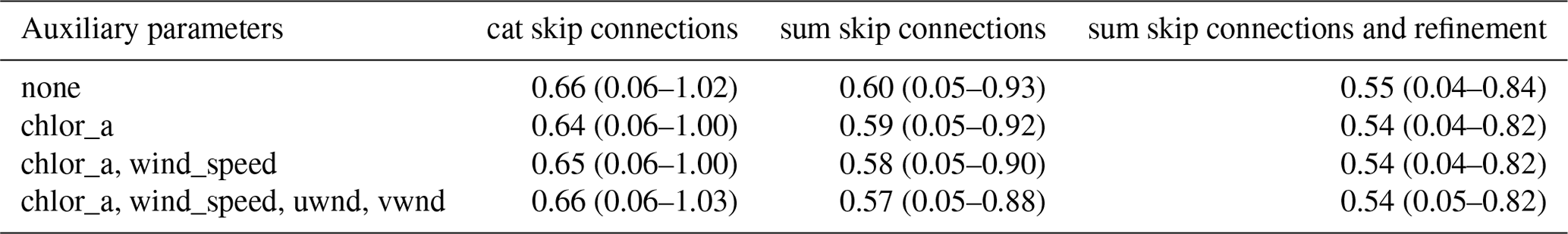
In Table 2 we present the test case for the Adriatic Sea with and without the skip connections and using the multivariate reconstruction. Besides the RMS error, this table also includes the 10 % and 90 % percentiles of the absolute value of the difference between the reconstructed data and the cross-validation data to provide a typical range of the error. In general, using chlorophyll a (or the wind fields) together with SST improved the results only marginally. The improvements were more consistent by using again the sum skip connection instead of the cat skip connection (in particular in conjunction with the additional refinement step). The analysis in the following uses the result of the lowest RMS, namely the reconstruction with sum skip connections and refinement and with the considered variables (chlorophyll a, the wind speed, zonal wind component and meridional wind component) as auxiliary parameters.
Table 2RMS errors (in ∘C) relative to the test dataset for different configurations (chlor_a: chlorophyll a, wind_speed: the wind speed, uwnd: zonal wind component, vwnd: meridional wind component). The two numbers in parentheses correspond to the 10 % and 90 % percentiles of the absolute value of the error.
When reconstructing sea surface temperature time series, it is often the case that for some days only very few data points are available. Figure 3 illustrates such a case, where a quite clear image was almost entirely masked as missing. DINCAE essentially produces an average SST (still using previous and next time frames) for the time of the year and a realistic spatial distribution of the expected error. The few pixels that are available have a relatively low error as expected, but the overall error structure looks quite realistic as the expected error increases significantly in the coastal areas (where the variability is higher and where the original satellite data are expected to be noisier). The reconstructed image matches the original image large-scale patterns relatively well, but as expected some small-scale structures are not reconstructed by the neural network. For this particular image, the RMS error (between the reconstructed data and the withheld data for cross-validation) is 0.43 ∘C and the 10 % and 90 % percentiles of the absolute value of the error are 0.05 and 0.63 ∘C, respectively.

Figure 3(a) The original MODIS SST; (b) MODIS SST with additional clouds for cross-validation; (c) the DINCAE reconstruction using the data from panel (b); (d) the expected error standard deviation of the DINCAE reconstruction. All panel values are in ∘C.
The detection of cloud pixels in the MODIS dataset is generally good, but Fig. 4 (for 17 September 2003) shows an example where some pixels were characterized as valid sea points while they are probably (at least partially) obscured by clouds, resulting in an unrealistically low sea surface temperature. For most analysis techniques derived from optimal interpolation, outliers like undetected clouds typically degrade the analyzed field in the vicinity of the spurious observations. The outlier also produced an artifact in the output of DINCAE, but it is interesting to note that in this case, the artifact did not spread spatially and the associated expected error has some elevated values indicating a potential issue at the location. The RMS error for this time instance is at 0.45 ∘C, similar to the previously shown image. The typical range of the absolute value of the error is 0.04–0.72 ∘C (10 % and 90 % percentiles).
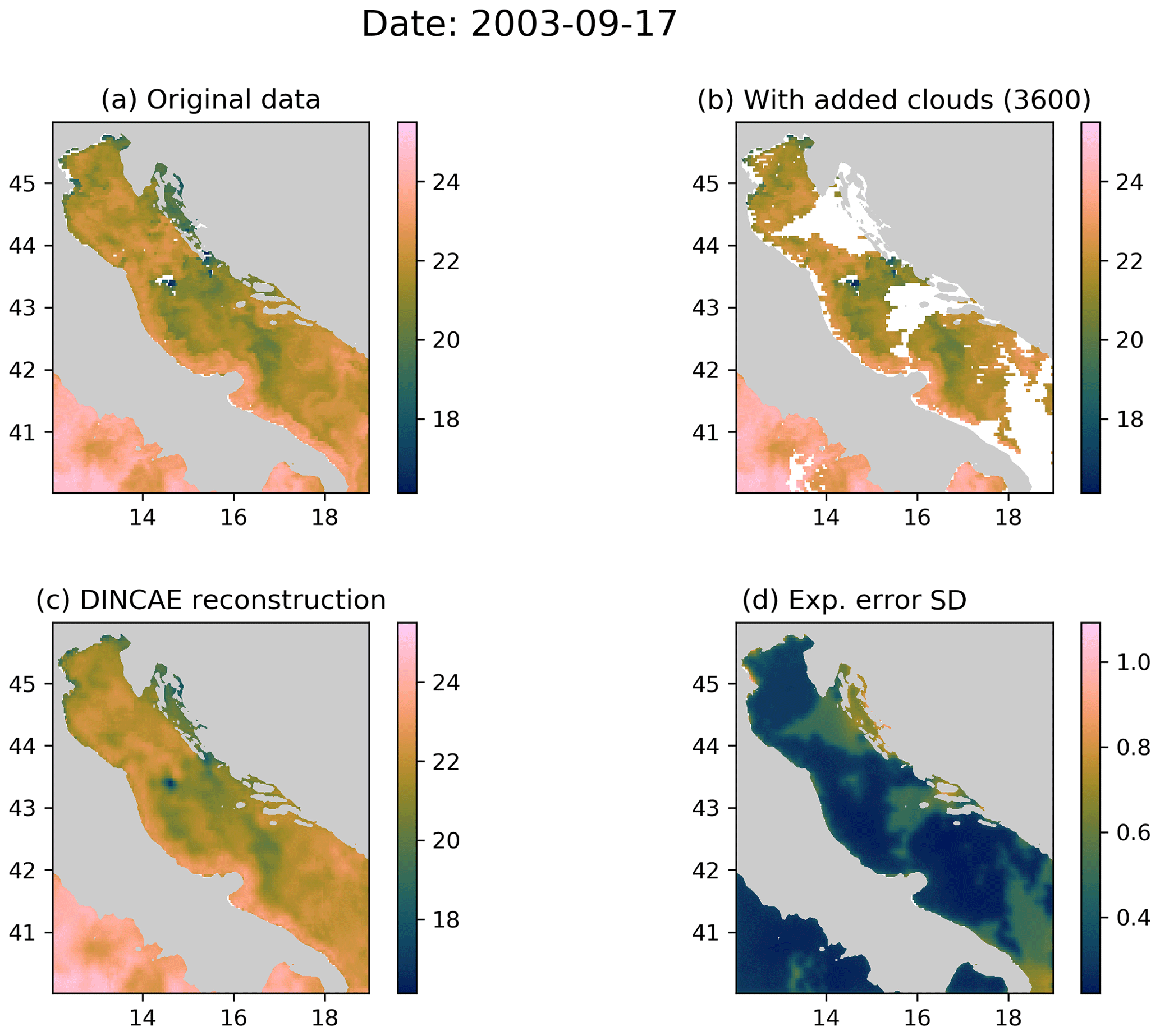
Figure 4(a) The original MODIS SST; (b) MODIS SST with additional clouds for cross-validation; (c) the DINCAE reconstruction using the data from panel (b); (d) the expected error standard deviation of the DINCAE reconstruction. All panel values are in ∘C.
A problem with techniques like optimal interpolation, variational analysis and to some degree also DINEOF is that the reconstruction smoothes out some small-scale features present in the initial data. For optimal interpolation and variational analysis, this smoothing is explicitly induced by using a specific correlation length. In EOF-based methods, this is related to the truncation of the EOFs series. In DINCAE, the input data are also compressed by a series of convolution and max pooling layers, and some smoothing is also expected, as in Fig. 4. Figure 5 shows an example where the initial data have almost no clouds and only few clouds are added for validation. The reconstructed field retains the filament and other small-scale structures. For this image, the RMS error (between the reconstructed data and the withheld data for cross-validation) is 0.55 ∘C and its typical range (as defined earlier) is 0.05 to 0.77 ∘C. The degree of smoothing can be quantified by the RMS difference of the reconstructed data and the input data (which is not an independent validation metric). This RMS difference is 0.15 ∘C, which is relatively low given the typical variability in sea surface temperature in this region.
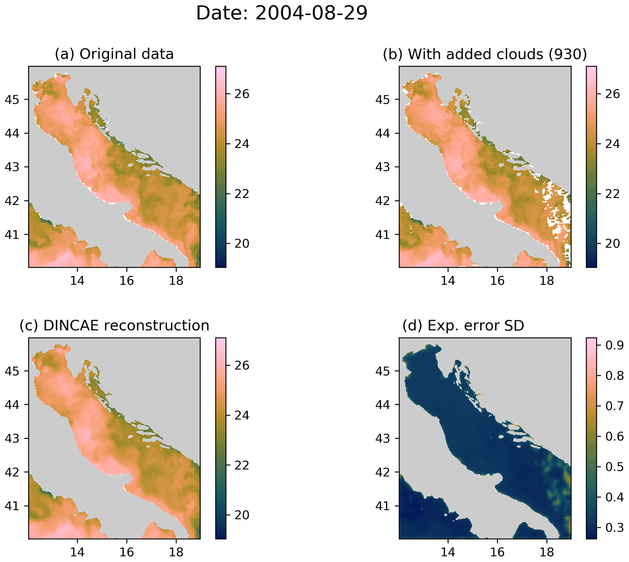
Figure 5(a) The original MODIS SST; (b) MODIS SST with additional clouds for cross-validation; (c) the DINCAE reconstruction using the data from panel (b); (d) the expected error standard deviation of the DINCAE reconstruction. All panel values are in ∘C.
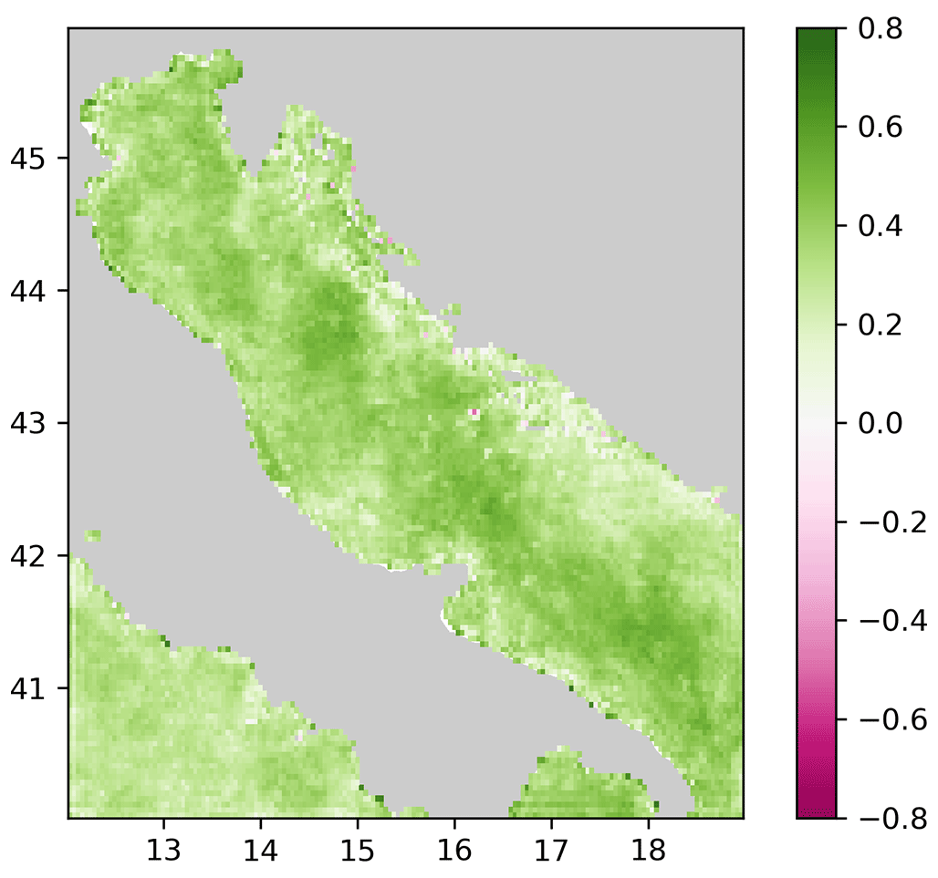
Figure 6Mean square error skill score of the monovariate reconstruction corresponding to DINCAE 1.0 and the multivariate case (considering all variables) and with an additional refinement step.
To assess the improvement spatially, the mean square skill score S is computed (Fig. 6) for every grid cell.
where MSEref is the mean square error of the monovariate reconstruction corresponding to DINCAE 1.0 relative to the validation dataset (per grid cell and averaging over time) and MSE is the mean square error of the multivariate case (considering all variables) and with an additional refinement step. The improvement is spatially quite consistent. The mean square error is mostly reduced in the northern and central parts of the Adriatic. Only on some isolated grid cells is a degradation observed. The skill score reflects the combined improvement due to the three changes implemented in this version: updated skip connections, refined step and multivariate reconstruction.
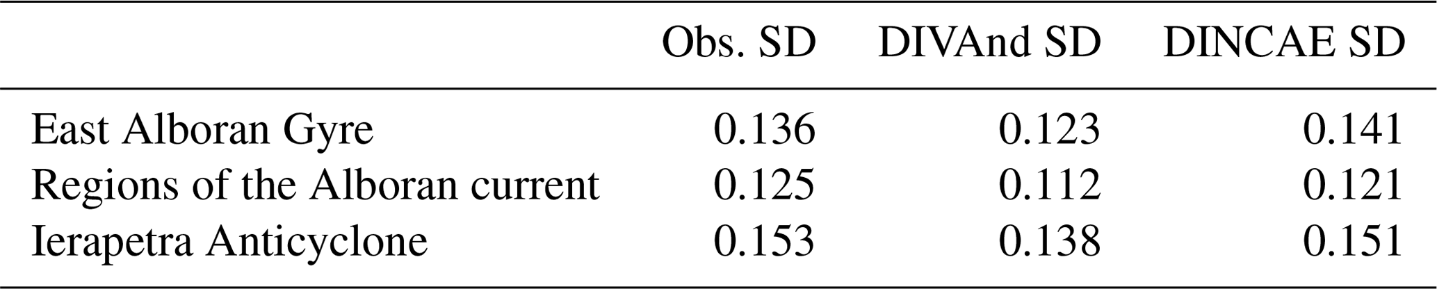
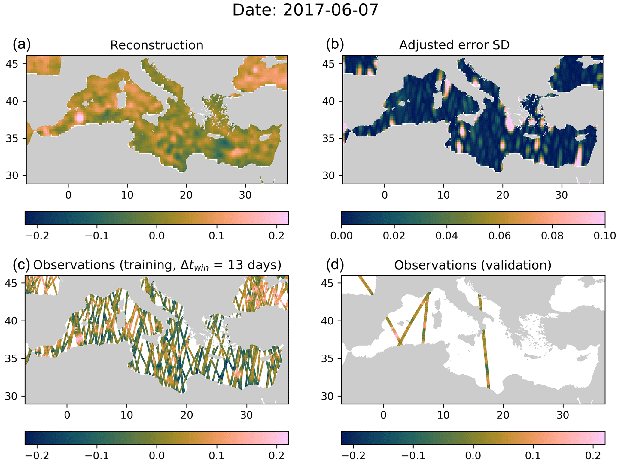
Figure 7Panel (a) Reconstructed SLA by DIVAnd, (b) expected error standard deviation by DIVAnd (with adjustment), (c) data used during training (partial) and (d) independent data for validation withheld during analysis. All panel values are in meters.

Figure 8Panel (a) Reconstructed SLA by DINCAE, (b) expected error standard deviation by DINCAE, (c) data used during training (partial) and (d) independent data for validation withheld during analysis. All panel values are in meters.
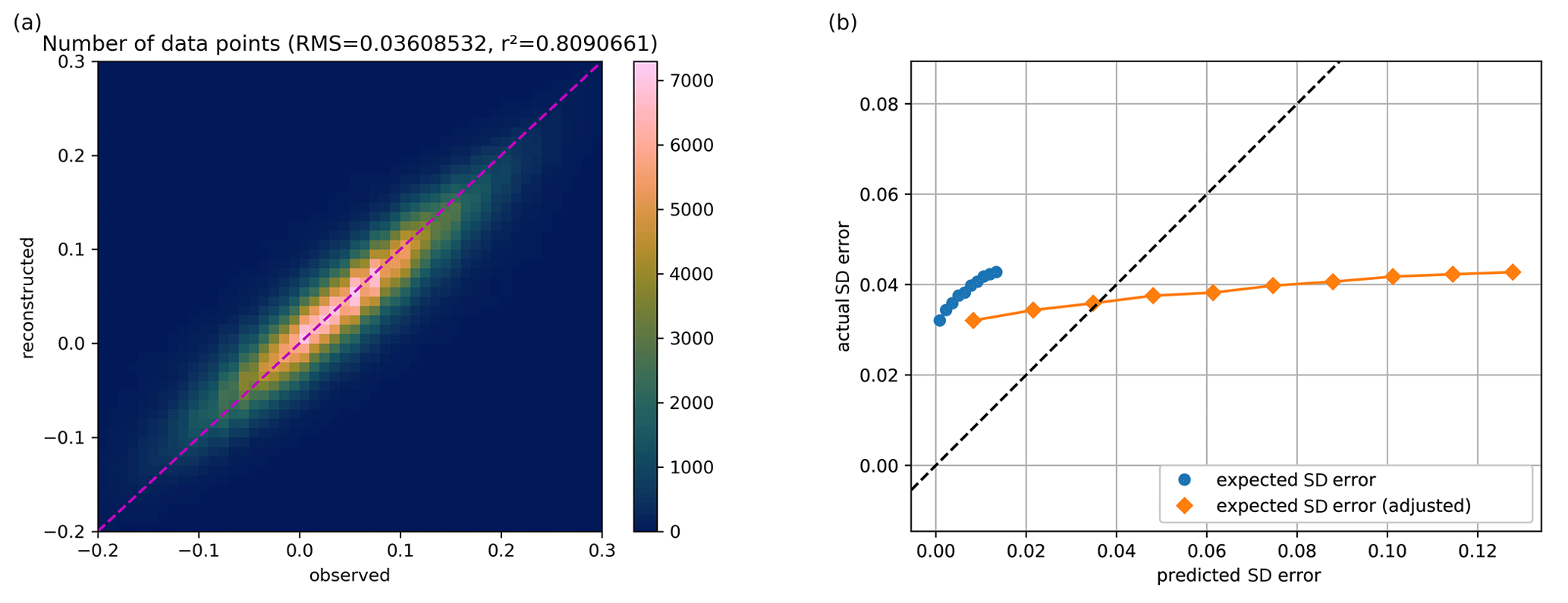
Figure 9(a) Altimetry observation from the test data versus the reconstructed values from DIVAnd (using only the training data). (b) Expected standard deviation of the reconstruction (before and after adjustment) relative to the actual standard deviation of the reconstructed misfit. The x and y axes of both plots are expressed in meters.
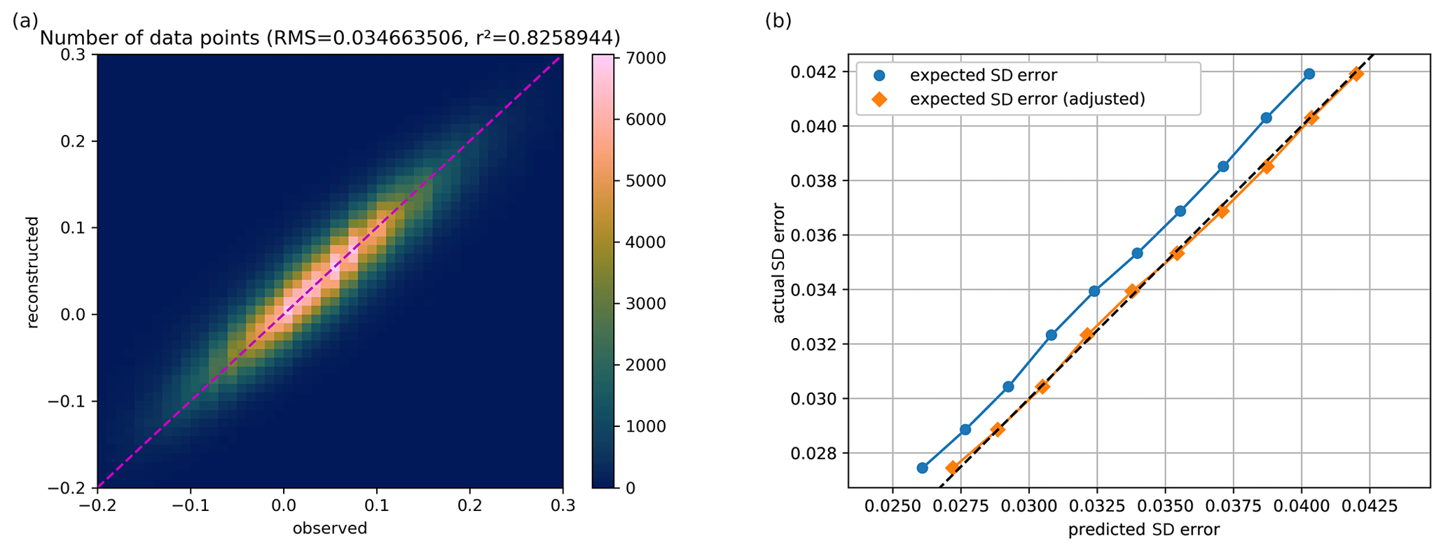
Figure 10(a) Altimetry observation from the test data versus the reconstructed values from DINCAE with SST as auxiliary parameter (using only the training data). (b) Expected standard deviation of the reconstruction (before and after adjustment) relative to the actual standard deviation of the reconstructed misfit. The x and y axes of both plots are expressed in meters.
5.2 Non-gridded data
The altimetry data is first gridded by the tool DIVAnd (Barth et al., 2014). The main parameters here are the spatial correlation length (in km), the temporal correlation scale (days), the error variance of the observations (normalized by the background error variance) and the duration of the time window Δtwin determining which observations are used to compute the reconstruction at the center of the time window.
All parameters of DIVAnd are also optimized using Bayesian minimization with an expected improvement in the acquisition function from minimizing the RMS error relative to the development datasets.
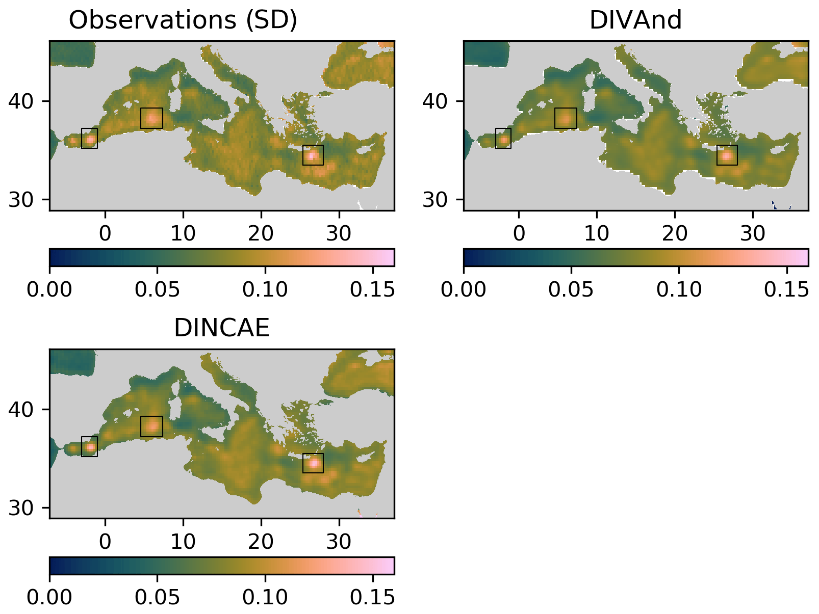
Figure 11Standard deviation of the sea-level anomaly for the DIVAnd method and DINCAE (including SST as auxiliary parameter).
The best DIVAnd result is obtained with a horizontal correlation length of 74.8 km, a temporal correlation length of 5.5 d, a time window of 13 d and a normalized error variance of the observations of 20.5. An example reconstruction for the date 7 June 2017 is illustrated in Fig. 7. The parameters are determined by Bayesian optimization, minimizing the error relative to the development dataset. The RMS error of the analysis for these parameters is 3.61 cm relative to the independent test dataset (Fig. 9).
The best performing neural network had a RMS error of 3.58 cm, which is only slightly better than results of DIVAnd (3.60 cm). When using the Mediterranean sea surface temperature as a co-variable we obtained a RMS error relative to the test dataset of 3.47 cm, resulting in a clearer advantage of the neural network approach. The left panels of Figs. 9 and 10 show on the x and y axes the observed altimetry (withheld during the analysis) and the corresponding reconstructed altimetry, respectively. The range of altimetry values from −20 to 30 cm was divided into 51 bins of 1 cm. The colors indicate the number of data points within each bin. For both reconstruction methods, the results scatter around the dashed line, which corresponds to the case where the reconstructed data correspond exactly to the observed altimetry. The eddy field of the DINCAE dataset is also quite similar to the one obtained from DIVAnd, but the anomalies of the structure are more pronounced in the DINCAE reconstruction (Fig. 8).
DINCAE and DIVAnd provide a field with the estimated expected error. For DIVAnd we used the “clever poor man's method” as described in Beckers et al. (2014), and the background error variance is estimated by fitting an empirical covariance based on a random pair of points binned by their distance (Thiebaux, 1986; Troupin et al., 2012). The estimated error variance is later adjusted by a factor to account for uncertainties in estimating the background error variance.
We made 10 categories of pixels based on the expected standard deviation error, evenly distributed between the 10 % and 90 % percentiles of the expected standard deviation error. For every category, we computed the actual RMS relative to the test dataset. Ideally this should correspond to the estimated expected error of the reconstruction (including the observational error). A global adjustment factor is also applied so that the average RMS error matches the mean expected error standard deviation, which is represented in the left panels of Figs. 9 and 10. This adjustment factor is also applied to Fig. 7b. The main advantage of DINCAE relative to DIVAnd is the improved estimate of the error variance of the results.
In summary, the accuracy of the DINCAE reconstruction is slightly better than the accuracy of the DIVAnd analysis. However, the main improvement of the DINCAE approach here is that the expected error variance of the analysis is much more reliable than the expected error variance of DIVAnd.
Figure 11 shows the standard deviation of the sea-level anomaly computed over the whole time period. From this figure, three areas in particular stand out corresponding (from east to west) to the East Alboran Gyre, regions of the Algerian current and the Ierapetra Anticyclone (annotated with the black rectangle in Fig. 11). The maximum standard deviation (related to the surface transport variability) for these three areas is shown in Table 3. The standard deviation is also computed from the satellite altimetry data considering all satellite observations falling within a given grid cell (excluding coastal grid cells with less than 10 observations). The standard deviation of the DINCAE reconstruction is in all three regions higher than the standard deviation for DIVAnd despite the DINCAE reconstruction having a lower RMS error than DIVAnd. In addition, the standard deviation of DINCAE is in general closer to the observed standard deviation.
In this paper, we discussed improvements of the previous described DINCAE method. The code has been extended to handle multi-variate reconstructions, which were also described in Han et al. (2020). We also found that multivariate reconstruction can improve the reconstruction, but the largest improvement was obtained by changing the structure of the neural network by using a newly implemented different type of skip connection and refinement pass. Interestingly, this type bears some similarities to the hierarchical multigrid method for solving partial differential equations. The handling of different types of satellite data was also improved. While most ocean satellite observations are gridded data (like sea surface temperature, ocean color, sea surface salinity and sea ice concentration), some parameters can only be inferred by nadir-looking satellites along tracks. For such non-gridded datasets, the first input layer is extended to handle such arbitrary location input data. We were able to show that the DINCAE method applied with altimetry data produces better reconstructions, but the main advantages are the significantly improved estimates of the expected reconstruction error variance. In this case, the DINCAE method compares favorably to the DIVAnd method (which is similar to optimal interpolation) in terms of reliability of the expected error variance, accuracy of the reconstruction relative to the test dataset and realism of the temporal standard deviation of the reconstruction assessed from the standard deviation of the observations.
The source code is released as open source under the terms of the GNU General Public Licence v3 (or, at your option, any later version) and available at the address https://github.com/gher-ulg/DINCAE.jl (last access: 9 March 2022) (https://doi.org/10.5281/zenodo.6342276, Barth, 2022). The sea surface temperature (MODIS Terra Level 3 SST Thermal IR Daily 4km Nighttime v2014.0, https://doi.org/10.5067/MODST-1D4N4, OBPG, 2015) is available via PO.DAAC (https://podaac.jpl.nasa.gov/, last access: 10 February 2022, JPL, NASA, USA), and wind speed (Cross-Calibrated Multi-Platform, CCMP, gridded surface vector winds) is available from Remote Sensing Systems (http://www.remss.com/measurements/ccmp/, last access: 19 July 2019). Chlorophyll a from Ocean Biology Processing Group, NASA, can be accessed at https://oceancolor.gsfc.nasa.gov/data/overview/ (last access: 18 September 2019). Altimetry data (dataset SEALEVEL_EUR_PHY_L3_MY_008_061) are made available by the Copernicus Marine Environment Monitoring Service (2020) (https://doi.org/10.48670/moi-00139). The L4 gridded SST over the Mediterranean is the NOAA Optimum Interpolation Degree Daily Sea Surface Temperature (OISST) Analysis, Version 2 available at https://www.ncei.noaa.gov/metadata/geoportal/rest/metadata/item/gov.noaa.ncdc:C00844/html (last access: 15 July 2020) (https://doi.org/10.7289/V5SQ8XB5, Reynolds et al., 2008).
AB designed and implemented the neural network. AB, AAA, CT and JMB contributed to the planning and discussions and to the writing of the manuscript.
The contact author has declared that neither they nor their co-authors have any competing interests.
Publisher's note: Copernicus Publications remains neutral with regard to jurisdictional claims in published maps and institutional affiliations.
The F.R.S.-FNRS (Fonds de la Recherche Scientifique de Belgique) is acknowledged for funding the position of Alexander Barth. This research was partly performed with funding from the Belgian Science Policy Office (BELSPO) STEREO III program in the framework of the MULTI-SYNC project (contract SR/00/359). Computational resources have been provided in part by the Consortium des Équipements de Calcul Intensif (CÉCI), funded by the F.R.S.-FNRS under Grant No. 2.5020.11 and by the Walloon Region. The authors also wish to thank the Julia community and in particular Deniz Yuret from Koç University (Istanbul, Turkey) for the Knet.jl package and Tim Besard (Julia Computing, Massachusetts, United States) for the CUDA.jl package, as well as the https://github.com/scikit-optimize/scikit-optimize/graphs/contributors (last access: 10 February 2022) developers of the python library scikit-optimize. We thank the reviewers for their careful reading of the manuscript and their constructive and insightful comments.
This research has been supported by the Fonds De La Recherche Scientifique – FNRS (grant no. 4768341) and by the Belgian Science Policy Office (BELSPO) STEREO III program in the framework of the MULTI-SYNC project (contract SR/00/359).
This paper was edited by Le Yu and reviewed by two anonymous referees.
Alvera-Azcárate, A., Barth, A., Beckers, J.-M., and Weisberg, R. H.: Multivariate reconstruction of missing data in sea surface temperature, chlorophyll and wind satellite field, J. Geophys. Res., 112, C03008, https://doi.org/10.1029/2006JC003660, 2007.
Atlas, R., Hoffman, R. N., Ardizzone, J., Leidner, S. M., Jusem, J. C., Smith, D. K., and Gombos, D.: A cross-calibrated, multiplatform ocean surface wind velocity product for meteorological and oceanographic applications, B. Am. Meteorol. Soc., 92, 157–174, https://doi.org/10.1175/2010BAMS2946.1, 2011.
Barth, A.: gher-ulg/DINCAE.jl: v2.0.0 (v2.0.0), Zenodo [code], https://doi.org/10.5281/zenodo.6342276, 2021.
Barth, A., Beckers, J.-M., Troupin, C., Alvera-Azcárate, A., and Vandenbulcke, L.: divand-1.0: n-dimensional variational data analysis for ocean observations, Geosci. Model Dev., 7, 225–241, https://doi.org/10.5194/gmd-7-225-2014, 2014.
Barth, A., Alvera-Azcárate, A., Licer, M., and Beckers, J.-M.: DINCAE 1.0: a convolutional neural network with error estimates to reconstruct sea surface temperature satellite observations, Geosci. Model Dev., 13, 1609–1622, https://doi.org/10.5194/gmd-13-1609-2020, 2020.
Beckers, J.-M., Barth, A., Troupin, C., and Alvera-Azcárate, A.: Approximate and efficient methods to assess error fields in spatial gridding with data interpolating variational analysis (DIVA), J. Atmos. Ocean. Technol., 31, 515–530, https://doi.org/10.1175/JTECH-D-13-00130.1, 2014.
Bezanson, J., Edelman, A., Karpinski, S., and Shah, V. B.: Julia: A fresh approach to numerical computing, SIAM Review, 59, 65–98, https://doi.org/10.1137/141000671, 2017.
Copernicus Marine Environment Monitoring Service, Collecte Localisation Satellites: European Seas along-track L3 sea surface heights reprocessed (1993–ongoing) tailored for data assimilation, Mercator Ocean International [data set], https://doi.org/10.48670/moi-00139, 2020.
Gong, Z., Zhong, P., and Hu, W.: Diversity in Machine Learning, IEEE Access, 7, 64323–64350, https://doi.org/10.1109/ACCESS.2019.2917620, 2019.
Han, Z., He, Y., Liu, G., and Perrie, W.: Application of DINCAE to Reconstruct the Gaps in Chlorophyll-a Satellite Observations in the South China Sea and West Philippine Sea, Remote Sensing, 12, 480, https://doi.org/10.3390/rs12030480, 2020.
He, K., Zhang, X., Ren, S., and Sun, J.: Deep Residual Learning for Image Recognition, in: 2016 IEEE Conference on Computer Vision and Pattern Recognition (CVPR), 770–778, https://doi.org/10.1109/CVPR.2016.90, 2016.
Head, T., Kumar, M., Nahrstaedt, H., Louppe, G., and Shcherbatyi, I.: scikit-optimize/scikit-optimize, Zenodo [code], https://doi.org/10.5281/zenodo.4014775, v0.8.1, 2020.
Hochreiter, S.: The Vanishing Gradient Problem During Learning Recurrent Neural Nets and Problem Solutions, Int. J. Uncertain. Fuzz., 6, 107–116, https://doi.org/10.1142/S0218488598000094, 1998.
Jones, D. R., Schonlau, M., and Welch, W.: Efficient Global Optimization of Expensive Black-Box Functions, J. Global Optim., 13, 455–492, https://doi.org/10.1023/A:1008306431147, 1998.
Kingma, D. P. and Ba, J.: Adam: A Method for Stochastic Optimization, CoRR, abs/1412.6980, arXiv [preprint], arXiv:1412.6980, 2014.
Liang, Y.-C., Mazloff, M. R., Rosso, I., Fang, S.-W., and Yu, J.-Y.: A Multivariate Empirical Orthogonal Function Method to Construct Nitrate Maps in the Southern Ocean, J. Atmos. Ocean. Technol., 35, 1505–1519, https://doi.org/10.1175/JTECH-D-18-0018.1, 2018.
Liu, H., Jiang, B., Xiao, Y., and Yang, C.: Coherent Semantic Attention for Image Inpainting, in: 2019 IEEE/CVF International Conference on Computer Vision (ICCV), 4169–4178, https://doi.org/10.1109/ICCV.2019.00427, 2019.
Long, J., Shelhamer, E., and Darrell, T.: Fully convolutional networks for semantic segmentation, in: 2015 IEEE Conference on Computer Vision and Pattern Recognition (CVPR), 3431–3440, https://doi.org/10.1109/CVPR.2015.7298965, 2015.
Mears, C. A., Scott, J., Wentz, F. J., Ricciardulli, L., Leidner, S. M., Hoffman, R., and Atlas, R.: A Near Real Time Version of the Cross Calibrated Multiplatform (CCMP) Ocean Surface Wind Velocity Data Set, J. Geophys. Res.-Oceans, 124, 6997–7010, https://doi.org/10.1029/2019JC015367, 2019.
Mockus, J., Tiesis, V., and Zilinskas, A.: The Application of Bayesian Methods for Seeking the Extremum, Towards Global Optimization, 2, 117–129, 1978.
Nardelli, B. B. and Santoleri, R.: Methods for the Reconstruction of Vertical Profiles from Surface Data: Multivariate Analyses, Residual GEM, and Variable Temporal Signals in the North Pacific Ocean, J. Atmos. Ocean. Tech., 22, 1762–1781, https://doi.org/10.1175/JTECH1792.1, 2005.
NASA Goddard Space Flight Center, Ocean Ecology Laboratory, and Ocean Biology Processing Group: Sea-viewing Wide Field-of-view Sensor (SeaWiFS) Ocean Color Data, NASA OB.DAAC [data set], https://doi.org/10.5067/ORBVIEW-2/SEAWIFS/L2/OC/2018, 2018.
National Centers for Environmental Information: Daily L4 Optimally Interpolated SST (OISST) In situ and AVHRR Analysis. Ver. 2.0. PO.DAAC, CA, USA [data set], https://doi.org/10.5067/GHAAO-4BC02, 2016.
OBPG: MODIS Terra Level 3 SST Thermal IR Daily 4km Nighttime v2014.0, Ver. 2014.0, PO.DAAC, CA, USA [data set], https://doi.org/10.5067/MODST-1D4N4, 2015.
Olmedo, E., Taupier-Letage, I., Turiel, A., and Alvera-Azcárate, A.: Improving SMOS Sea Surface Salinity in the Western Mediterranean Sea through multivariate and multifractal analysis, Remote Sensing, 10, 485, https://doi.org/10.3390/rs10030485, 2018.
Olmedo, E., González-Haro, C., Hoareau, N., Umbert, M., González-Gambau, V., Martínez, J., Gabarró, C., and Turiel, A.: Nine years of SMOS sea surface salinity global maps at the Barcelona Expert Center, Earth Syst. Sci. Data, 13, 857–888, https://doi.org/10.5194/essd-13-857-2021, 2021.
Reynolds, R. W., Smith, T. M., Liu, C., Chelton, D. B., Casey, K. S., and Schlax, M. G.: Daily High-resolution Blended Analyses for sea surface temperature, J. Climate, 20, 5473–5496, https://doi.org/10.1175/2007JCLI1824.1, 2007.
Reynolds, R. W., Banzon, V. F., and NOAA CDR Program: NOAA Optimum Interpolation 1/4 Degree Daily Sea Surface Temperature (OISST) Analysis, Version 2, NOAA National Centers for Environmental Information [data set], https://doi.org/10.7289/V5SQ8XB5, 2008.
Ronneberger, O., Fischer, P., and Brox, T.: U-Net: Convolutional Networks for Biomedical Image Segmentation, in: Medical Image Computing and Computer-Assisted Intervention – MICCAI 2015, edited by: Navab, N., Hornegger, J., Wells, W. M., and Frangi, A. F., 234–241, Springer International Publishing, Cham, https://doi.org/10.1007/978-3-319-24574-4_28, 2015.
Snoek, J., Larochelle, H., and Adams, R. P.: Practical Bayesian optimization of machine learning algorithms, in: Advances in Neural Information Processing Systems, 2951–2959, 2012.
Szegedy, C., Liu, W., Jia, Y., Sermanet, P., Reed, S., Anguelov, D., Erhan, D., Vanhoucke, V., and Rabinovich, A.: Going Deeper with Convolutions, in: Computer Vision and Pattern Recognition (CVPR), arXiv [preprint], arXiv:1409.4842, 2015.
Thiebaux, J.: Anisotropic correlation functions for Objective Analysis., Mon. Weather Rev., 104, 994–1002, https://doi.org/10.1175/1520-0493(1976)104<0994:ACFFOA>2.0.CO;2, 1986.
Troupin, C., Barth, A., Sirjacobs, D., Ouberdous, M., Brankart, J.-M., Brasseur, P., Rixen, M., Alvera-Azcárate, A., Belounis, M., Capet, A., Lenartz, F., Toussaint, M.-E., and Beckers, J.-M.: Generation of analysis and consistent error fields using the Data Interpolating Variational Analysis (DIVA), Ocean Modell., 52–53, 90–101, https://doi.org/10.1016/j.ocemod.2012.05.002, 2012.
Wentz, F., Scott, J., Hoffman, R., Leidner, M., Atlas, R., and Ardizzone, J.: Remote Sensing Systems Cross-Calibrated Multi-Platform (CCMP) 6-hourly ocean vector wind analysis product on 0.25 deg grid, Version 2.0, Remote Sensing Systems [data set], Santa Rosa, CA, http://www.remss.com/measurements/ccmp, last access: 19 July 2019.
Wylie, D., Jackson, D. L., Menzel, W. P., and Bates, J. J.: Trends in Global Cloud Cover in Two Decades of HIRS Observations, J. Climate, 18, 3021–3031, https://doi.org/10.1175/JCLI3461.1, 2005.
Yuret, D.: Knet: beginning deep learning with 100 lines of Julia, 30th Conference on Neural Information Processing Systems (NIPS 2016), Barcelona, Spain, 2016.
Zhang, Z., Stanev, E. V., and Grayek, S.: Reconstruction of the Basin-Wide Sea-Level Variability in the North Sea Using Coastal Data and Generative Adversarial Networks, J. Geophys. Res.-Oceans, 125, e2020JC016402, https://doi.org/10.1029/2020JC016402, 2020.